CONTACT

Remi JedwabDepartment of EconomicsGeorge Washington Universityjedwab@gwu.edu

WORKI NG PAPER #16 / OCTOBER 2014

MALTHUSIAN DYNAMICS AND THE RISE OF THE POOR MEGACITY+ REMI JEDWAB AND DIETRICH VOLLRATH

ABSTRACT

The largest cities in the world today lie mainly in relatively poor countries, which is a departure from historical

experience, when the largest cities were typically found in the richest places. Further, these poor mega-cities have grown

through high rates of urban natural increase, as opposed to the in-migration that drove historical urbanization. In this

paper we provide an explanation for the rise of these poor mega-cities and their departure from the historical norms.

Combining models of urban agglomeration and congestion with Malthusian models of endogenous population, we

show that cities can exert Malthusian forces on living standards. Poor mega-cities have grown because their rapid rate of

natural increase exerts a downward force on urban wages, which ensures that natural increase remains high, the mega-

cities remain poor, and their size is unrelated to productivity. In comparison, richmega-cities of the past had low rates

of natural increase, ensuring that they could take advantage of agglomeration technologies, and city growth occurred

in response to productivity improvements. Our work shows that Malthusian forces do not disappear just because an

economy urbanizes, and that urban Malthusianism combines with rapid urban population growth to drive developing

poor mega-cities towards stagnation even if they do not face limits to their resource stocks.

Dietrich VollrathDepartment of EconomicsUniversity of Houstondevollrath@uh.edu

We would like to thank seminar audiences at EUDN (Berlin), George Mason-George Washington Economic History Workshop, George Washington (IIEP and SAGE), George Washington University Urban Day, Goethe University of Frankfurt, Harvard Kennedy School (NEUDC), Michigan, Minnesota (MIEDC), NYU Urbanization Project, Oxford (CSAE), Paris School of Economics (seminar and RSUE Workshop), University of California-Los Angeles (PACDEV), University Paris 1, the Urban Economic Association meetings (Atlanta), U.S. Department of State (Strategic Consequences of Urbanization in Sub-Saharan Africa to 2025) and World Bank-George Washington University Conference on Urbanization and Poverty Reduction 2013 for very helpful comments. We thank the Institute for International Economic Policy at George Washington University for financial assistance.

PHOTO BY FRED R VIA FLICKR

1. INTRODUCTION

Urbanization has gone hand in hand with economic growth throughout history, and the

majority of world population now lives in cities. However, post-war developing countries

have urbanized in a fundamentally different manner compared to the historical experience of

developed countries. Specifically, the post-war period has seen the rise of poor mega-cities

in developing nations, which we document in detail below. Delhi, Dhaka, Kinshasa, Karachi,

and Lagos are some of the very largest urban agglomerations on the planet today, each with

over 10 million inhabitants. Only six of the currently largest 30 cities (Tokyo, New York, Los

Angeles, Paris, Osaka, and London) today are in high income countries. The prevalence of poor

mega-cities today runs counter to historical experience. In the first half of the 20th century,

the very largest urban agglomerations in the world were all in the most advanced economies

(e.g. New York, London, Paris, Berlin, Chicago) with only a few major cities in poor countries,

like Mumbai, reaching even one-fourth of their size.

The mega-cities of today’s developing world are also unlike their historical peers in that their

massive size is not indicative of rapid economic growth or higher living standards. For the

poorest countries, urbanization rates in 2010 are roughly 10 percentage points higher than

in 1950, and 20 percentage points higher than they were in 1910 for identical levels of GDP

per capita. Developing countries of today are urbanizing into poor mega-cities that do not

appear to be able to take advantage of the externalities or agglomeration economies of their

rich-country peers.

Our aim in this paper is to provide an explanation for the rise of these poor mega-cities, and

why they differ from the historical experience of urbanization and rapid economic growth.

We propose that these mega-cities grew in poverty - and tend to remain mired in poverty -

because of what we characterize as urban Malthusian forces. To describe these forces, we build

a model that combines the insights of Malthusian models of endogenous population growth

(Ashraf & Galor, 2011; Galor & Weil, 2000) with the urban literature on equilibrium city size

(Duranton & Puga, 2004; Duranton, 2013). The Malthusian literature describes how limited

resources will tend to restrict living standards to some subsistence level under the assumption

that population growth responds positively to living standards. The urban literature captures

the tension between the positive effects of agglomeration economies and the negative effects

of congestion to find that urban wages display an inverted-U shape with respect to city size. For

sufficiently large cities, the urban congestion effect dominates and this generates the typical

Malthusian relationship of population and living standards.

Urban agglomerations thus can become “too big”, at which point they become subject to the

same type of Malthusian pressures that arise in models featuring fixed stocks of resources.

Here, rather than limited agricultural land, the Malthusian pressures arise because urban

congestion overwhelms any positive agglomeration economies. Sufficiently rapid city growth

1

can drive down living standards.

Within this model, we are able to distinguish a poor mega-city equilibrium that differs from the

historical equilibrium. Poor mega-cities arise and persist because their rates of natural increase

are very high, which leads to large absolute size but also keeps living standards low through the

urban Malthusian effects. Low living standards ensure that rates of natural increase remain

high, and hence the poor mega-cities end up growing without bound. In particular, their

growth is unrelated to productivity changes in the formal urban sector (which has positive

agglomeration economies), as their size ensures that this technology is no longer viable due to

congestion effects. In comparison, the historical equilibrium involves cities with low rates of

natural increase, which allows them to maintain relatively high wages, which in turn reinforces

the low rate of natural increase. These cities continue to use the formal urban technology, and

grow in size precisely because of productivity increases with that technology.

This poor mega-city equilibrium differs from the historic experience because of their urban rate

of natural increase is so large. We document more fully below that for modern developing

nations, cities have rates of natural increase that are well above those seen historically. In

particular, city mortality rates are quite low in developing countries today, well below levels

seen at comparable periods of development for rich nations. These low mortality rates arose

in the post-war period due to the epidemiological transition, which brought crude death rates

in these cities down close to rich country levels. Crude birth rates in the poor mega-cities

remained large, and similar to historical rates for large cities. The combination of the birth

rates with the very low mortality rates within poor mega-cities implied a strongly positive

urban rate of natural increase in these developing nations. In terms of our model, this high

observed rate of natural increase meant rapid internal city growth, and pushed these cities

into the poor mega-city equilibrium.

Because of the Malthusian nature of urban areas, our model has similar implications to typical

Malthusian models. Lower congestion costs act like an expansion of the resource base in

standard Malthusian models, expanding the size of cities before eventually returning to the

subsistence living standard. Moreover, lower mortality rates and/or higher fertility rates are

“bad” in this model, because they push down the subsistence living standard. The poor mega-

city equilibrium is one that arises perversely because of the success of interventions that limited

urban mortality rates while urban fertility remains relatively high. In this, our work is similar

to others that emphasize the negative effect of mortality interventions and/or the positive

impacts of mortality increases (Acemoglu & Johnson, 2007; Young, 2005).

The origin of poor mega-cities is certainly not mono-causal, and our explanation involving

Malthusian effects should be thought of as a complement to those involving changes in

urban transportation and housing technologies (i.e. the ability to build out or build up),

changes in preferences towards urban areas, urban-biased policies, or others. One advantage

of our explanation is that it is generalized, in the sense that all urban areas are likely to

2

have the agglomeration and congestion effects driving our results. Other explanations would

exacerbate or mitigate the effects we are discussing here, but do not rule out ours.

The main contribution of our paper is to explain the conditions under which these poor mega-

cities will arise, and to describe what their future may look like. In addition to this, our work

adds to the literature on the effects of demography on economic growth in general. Population

growth promotes economic growth if high population densities encourage human capital

accumulation or technological progress (Kremer, 1993; Becker, Glaeser & Murphy, 1999;

Lagerlof, 2003). In the urban setting we consider, there are positive impacts of population

growth due to agglomeration effects - but only over some range of population size. Population

growth also induces congestion effects, which negatively affects living standards, similar

to unified growth models that have a fixed resource (i.e. agricultural land) as part of the

production process (Galor & Weil, 1999, 2000; Strulik & Weisdorf, 2008; Galor, 2011). Our

work shows that the negative Malthusian effects need not arise because of natural resource

limits, but rather due to the nature of urbanization. Significantly, this implies that Malthusian

forces need not disappear as economies develop. Those forces remain operational even though

agriculture and/or resource extraction cease to be significant sectors of production.

This paper is close in subject matter to Voigtländer & Voth (2013a), who study the possibility

of multiple equilibria based on the urbanization process in historical Europe and China, but

do not consider the modern arrival of poor mega-cities in the developing world. In terms of

mechanisms, they introduce a non-linearity in mortality rates tied to a threshold urbanization

rate, and thus an exogenous shock like the Black Death leads allows Europe to move to a better

equilibrium. In comparison, our model introduces an explicit Malthusian force in city size, and

the equilibrium that a city ends up is not a result of an exogenous shock to city size.

Our work also is linked to studies that look at the effect of mortality changes on population

and economic growth (Acemoglu & Johnson, 2007; Bleakley, 2007; Bleakley & Lange, 2009;

Bleakley, 2010; Cutler et al., 2010). Other studies have looked at the effects of unexpected

decreases in population on development (Young, 2005; Voigtländer & Voth, 2009; Ashraf,

Weil & Wilde, 2011; Voigtländer & Voth, 2013a,b). Relative to those works, we consider the

implications of unexpected population increases, specifically from the perspective of cities.

The few papers that have looked at cities examined how urbanization rates affected the

demographic transition and developemtn (Sato & Yamamoto, 2005; Sato, 2007; Voigtländer

& Voth, 2013b). In contrast, our model of urban Malthusianism highlights the fact that the

absolute size of urban agglomerations is a crucial component of developement.

Glaeser (2013) begins with the same set of motivating facts regarding poor mega-cities, but

looks at them in a different light. His paper focuses on the internal institutional structure

that prevents mega-cities from reducing the overwhelming congestion effects of their size,

examining the trade-off between disorder and dictatorship. His model does not consider the

unique demographics leading to the origin of these mega-cities.

3

In the following section we document more fully the rise of poor mega-cities in the developing

world, and the underlying demographic features of these cities. Then, with those stylized facts

in place, we present our model of urban Malthusian dynamics, showing how an economy may

find itself in an equilibrium with poor mega-cities. We then compare this equilibrium to the

situation seen in historical European development.

2. FACTS ON THE RISE OF POOR MEGA-CITIES

Table 1 shows the largest 30 cities in select years from 1700 to 2015 (Chandler, 1987; United

Nations, 2014). In 1700, the largest cities were under 1 million persons in size, with Istanbul,

Tokyo, and Beijing all at around 700,000 inhabitants. While small in absolute size, the largest

cities in 1700 were generally located in the most economically advanced areas of the world

in that period. While London and Amsterdam had wages that were high relative to other

European cities and the rest of the world, cities such as Beijing, Tokyo, and Istanbul all had

wages equivalent to those found in cities such as Paris and Naples (Allen, 2001; Allen et al.,

2011; Özmucur & Pamuk, 2002).

By 1900, the nature of the list of largest cities changed along several dimensions. First, the

absolute sizes were roughly an order of magnitude larger than in 1700. Urban growth, like

population growth in the period 1700–1900, was extrodinarily rapid. In 1900, the largest

city was London, with 6.5 million inhabitants, and there were 17 cities with over one million

residents. Second, the cities that dominate this list were the leading cities from the richest

countries. London, New York, Paris, Berlin, Chicago, Vienna, and Tokyo are all found on

the list. Further down, we see Manchester, Birmingham, Philadelphia, Boston, Liverpool,

Hamburg, and the Ruhr area, all centers of industrialization in the western world.

There were several large agglomerations in relatively poor places in 1900: Beijing, Kolkata,

Mumbai, and Rio de Janeiro. But note that none approached the size of the leaders like London

or New York. Comparing 1900 to 1700, one can also see that their growth in this period was

not on the same scale as the richer cities. Beijing increased only from 700,000 to 1.1 million in

the same 200 years that London went from 600,000 to 6.5 million. Istanbul had only 900,000

residents in 1900, up from 700,000 in 1700. Rapid city growth by 1900 was a feature of rich

countries, not of poor ones.

This trend continued into 1950, where the top cities remained those in relatively advanced

nations. New York, Tokyo, and London were the largest agglomerations, but the remainder of

the list contains Chicago, Los Angeles, Detroit, Boston, Birmingham, and Manchester. What

we can see, though, is the very beginnings of mega-city growth in relatively poor countries.

Kolkata and Shanghai both had more than four million inhabitants in 1950, putting them in

the top 10 cities in the world in 1950. Rio de Janeiro, Mexico City, Mumbai, Cairo, and Beijing

were all over 2 million inhabitants, reflecting incredible growth for most of them from earlier

4

periods.

By 2015, notice that the nature of the largest cities is dramatically different. First, the absolute

scale of cities are 3-5 times larger than in 1950, again representing the combination of rapid

population growth and increased urbanization rates. Second, the composition of the list is now

dominated by cities in poor countries. Only Tokyo, New York, Los Angeles, Paris, Osaka, and

London are in what we would typically term rich countries. Instead we see cities such as Delhi,

Sao Paulo, Mumbai, and Mexico City. Countries that rank at the bottom in development levels

have cities present on this list, such as Dhaka (Bangladesh), Manila (Philippines), Karachi

(Pakistan), Lagos (Nigeria), and Kinshasa (DRC). Each of those poor cities have at least 11

million people, making them larger in absolute size than nearly every city in the world in

1950.

The shift of the largest cities in the world from rich countries to poor countries can be more

easily seen in Figure 1. This plots the number of cities with more than one million inhabitants

for two groups, developed countries (based on their 2013 GDP per capita) and developing

countries. As can be seen, in 1700 there were no cities in either set of countries with one

million inhabitants. In 1900 and 1950 nearly all of the million-plus sized cities were in

currently developed nations. This switches dramatically between 1950 and 2015, however,

and this reversal is projected to increase well into this century. By 2030, the UN expects there

to be close to 400 million-resident cities in developing countries, versus only 250 in developed

nations.1 Most of the mega-cities of the world are now, and will continue to be, in relatively

poor countries, representing a significant switch in the pattern seen historically.

This change in the composition of the largest cities is only going to be exacerbated in the

future. Column (1) of Table 2 shows the 30 largest agglomerations in 2015 ranked by their

projected growth rate. As can be seen, this list is led by the primarily by poor mega-cities such

as Lagos (Nigeria), Kinshasa (DRC), and Dhaka (Bangladesh). If we turn instead to column

(2), this ranks all cities over 5 million inhabitants by their projected growth rate from 2015-

2030. Here we see that the fastest growing cities are again some of the poorest; Dar es Salaam

(Tanzania), Luanda (Angola), and Abidjan (Ivory Coast) are all expected to grow at over 3 per

cent per year, which will take them into the top 30 in absolute city size by 2030.

It is interesting to compare these projected growth rates of poor mega-cities with the growth

rates of existing rich mega-cities. Looking at the bottom of column (1) in Table 2, one can

find current top-30 mega-cities like London, Paris, New York, and Tokyo. Their growth rates

are all under 1%, and Tokyo is expected to actually shrink in size. These cities will be passed

by a number of poor mega-cities in absolute size over the next two decades, as their growth

has slown down over time and they appear headed for a steady state size. One can see this by

1We find a similar pattern if we only consider agglomerations over 5 million people, or the absolute populationliving in mega-cities (defined either as greater than 1 million or greater than 5 million), or the proportion ofpopulation living in mega-cities (again, for either more than 1 million or more than 5 million).

5

looking at column (2), which ranks all cities by their projected growth rate, and none of the

rich wold cities make the list.

This rise of poor mega-cities is reflected in shifts in the relationship between income per capita

and urbanization over time. Figure 2 plots the urbanization rate against GDP per capita for

three years, 1910, 1950 and 2010, along with linear fits to the relationship. As can be seen,

there has been a distinct shift up in the relationship over time. That is, urbanization rates

are much higher in 2010 for any given level of income per capita than they were in 1910 or

1950.

In 1910, the poorest countries of the world (i.e. log GDP per capita less than 7, roughly

$1,100) all had urbanization rates at or below 10%. By 1950 countries with the same low

level of income per capita had urbanization rates of around 20%. But by 2010, though,

the urbanization rate for this level of income is around 30%, with several outliers reaching

urbanization rates of nearly 50%.

For each year, the positive relationship of income per capita and urbanization remains, and

the slopes are statistically indistinguishable from each other. But clearly there has been a

shift in the level of this relationship. A different way of interpreting the leftward shift over

time in Figure 2 is that countries tend to be poorer in 2010 than in 1950 or 1910 for a given

urbanization rate. The combination of the information in Figures 1 and 2, as well as Table 1

shows us that mega-cities have grown disproportionately large in the very poorest countries.

Urbanization does not imply the same level of living standards that it did in the past.

3. THE DEMOGRAPHICS OF POOR MEGA-CITIES

The rapid population growth of poor mega-cities is different from that experienced during

earlier urbanization episodes. The poor mega-cities of today grow in large part through natural

increase, along with in-migration. Historically, in-migration tended to be a more important

source of new city dwellers as the rates of natural increase were quite low in urban areas,

typically because of high mortality rates.

This can be seen clearly if we compare the crude birth rate (CBR) and crude death rate (CDR)

of cities across different historical eras. In Figure 3 we plot CBR against CDR for a collection

of 14 pre-Industrial Revolution cities, such as ancient Rome, Renaissance Florence, London in

the 17th century, and Delhi in the 19th century. As can be seen, the cities all lie on or below the

45-degree line, indicating that birth rates were below death rates, and the cities experienced

negative rates of natural increase. Their growth could occur only through in-migration. Those

that do lie above the line (Berlin in the 1810s, Beijing in the 19th century, Delhi in the 19th

century) are barely above the line, and the crude rate of natural increase is very low.

These data do not give a full account of the effects of major disease outbreaks. Florence in

6

the 15th century (after the plague) has a slightly positive crude rate of natural increase, lying

above the 45-degree line. However, in 1348 during the plague years the CDR in Florence was

roughly 500, and similar crude death rates of 25-50% of population were seen across European

cities (Miskimin, 1975). All the points in Figure 3 thus represent “normal” periods, but each

was at times afflicted by similar shocks to mortality, so that the average CDR over long periods

of time was likely higher than indicated. Overall, pre-industrial cities tended to experience

negative rates of natural increase, and grew only through in-migration.

Figure 4 shows similar data for cities during the Industrial Revolution (with red crosses

representing the prior information). Here we can see that while crude birth rates are roughly

on the same level with the pre-industrial era, the crude death rate has declined slightly. There

remain several cities below the 45-degree line (e.g. London in the 1750s, Amsterdam in the

1850s, Tokyo in the 1900s) but most cities are now experiencing some small positive rate of

natural increase. These cities were growing not only through in-migration, but now in part

through some increase in their own population. Note, though, that crude death rates remain

in the range of roughly 15-40 for these cities.

If we now turn to the post-war period, and the 1960s in particular, we can see in Figure 5

a distinct change in city demographics. Again, the earlier data is plotted with crosses for

comparison. Focus first on the collection of relatively rich cities in the lower left, such as

London, New York, Paris, and Tokyo. These cities are already very large, as shown in Table 1.

But their crude birth rates have fallen along with their crude death rates, and so their rate of

natural increase (CBR minus CDR) remains relatively muted, similar in size to that seen during

the Industrial Revolution. Overall, it is apparent from Figures 3-5 that historically cities were

moving “down” the 45 degree line as they grew, but never straying far from it. Natural increase

in these cities was never particularly large, even if the absolute size of CDR and CBR were. As

these places developed, the CDR and CBR drop in tandem, keeping the rate of natural increase

small.

In comparison are the nascent poor mega-cities of the developing world in the upper left of the

figure, well above the 45 degree line, and distinctly different from the historical pattern. In

the immediate post-war era these cities differ from earlier eras in one very distinct way: their

crude death rates are very low. Lagos, Karachi, and Jakarta all have crude death rates in the

1960s that are roughly similar to those seen in London, New York, or Paris in the same year.

The crude birth rates in these cities are large, but not substantially larger than those seen in

pre-industrial or industrial revolution era cities. Developing cities in the 1960s were “shifted

left” in Figure 5 compared to their historical peers. This led to very large rates of natural

increase compared to the prior norms for emerging mega-cities, and this is driven primarily

by the substantially lower crude death rates. For example, in the African mega-cities in the

figure, crude rates of natural increase are roughly 30, or 3% per year. Absent migration, this

implies that these cities double in size roughly every 20 years.

7

This difference continues into the more contemporary period of the 2000s, which is plotted

in Figure 6. Rich mega-cities such as New York, Paris, and Tokyo remain in roughly the same

position as in the 1960s, with low crude death and crude birth rates. The poor mega-cities

of the developing world have also shifted down to lower crude birth rates, and this makes

it more apparent that crude birth rates in these poor mega-cities do not differ from those in

earlier eras. However, the crude death rates in these poor mega-cities are much lower than

the historical comparisons, for the most part falling below 10 per thousand. Thus in the 2000s

poor mega-cities continued to have extremely rapid rates of natural increase. These findings

are consistent with those of Jedwab, Christiaensen & Gindelsky (2014), who document the

high rates of natural increase for modern developing countries in the urban sector as a whole,

as opposed to the specific cities we examine.

The deviation of the developing countries in Figures 5 and 6 from the historical norms of

low rates of urban natural increase appears due, in large part, to what Acemoglu & Johnson

(2007) refer to as the international epidemiological transition. Following 1940, there was a

rapid improvement in health (particularly in infant mortality) in many developing countries.

This was due to the availability of new treatments (e.g. antibiotics) and vaccines, a world-wide

effort by the World Health Orgnization and others to provide access to those new treatments

and vaccines, and a focus on rapid dissemination of public health innovations to developing

countries (Stolnitz, 1955; Davis, 1956; Preston, 1975). Combined, these changes led to

substantial decreases in crude death rates. In turn, health conditions in many developing

countries in the post-war era are much better than were conditions in currently developed

nations at similar stages of development (Acemoglu & Johnson, 2007).

As the epidemiological transition raised crude rates of natural increase in developing mega-

cities, it brought those rates up to the levels seen in rural areas, another anomaly compared

to historical experience. In the Industrial Revolution, the crude rate of natural increase in the

cities we study was only 3.4 per thousand. For the same time periods, the rural crude rate of

natural increase in the respective countries averaged 15.4, the difference coming both through

higher birth rates and lower death rates in rural areas (see Web Appendix for sources). By the

1960’s however, the crude rate of natural increase in the largest cities was 22.6, on average,

with nearly all of that increase coming through a decline in the CDR. During the same period,

the crude rate of natural increase in rural areas in the same countries was 22.3. So while rates

of natural increase were larger in both mega-cities and rural areas, the advance in mega-cities

was so substantial that by the 1960s these cities had rates matching those of rural areas.

This can be seen most clearly in Figure 7. Here we plot the urban CRNI for historical and

modern cities from the prior figures against the rural CRNI for the associated country in the

same time period. A lack of sufficient data on rural areas limits this sample to fewer cities than

we have in the prior figures. The observations in the figure are distinguished as developing

based on current World Bank classifications.

8

As can be seen, observations from developed countries lie almost exclusively below the 45

degree line, indicating that urban CRNI was well below rural CRNI. The exceptions to this

have very low levels of CRNI in both areas, and are for cities such as New York, Los Angeles,

and Paris in the 2000s. The remaining points, which cover London in the 17th century, a

number of European cities in the 19th century, and other rich cities in the early part of the

20th century, all lie well below the line. Rural rates of natural increase were much higher than

urban rates in these historical cities.

In constrast, the poor mega-cities in developing countries all tend to cluster near the 45 degree

line, indicating similar rates of urban and rural CRNI. For many cities the urban CRNI is higher

than in the associated rural area. The implication of this is that for these developing cities

urbanization did not exert any downward pressure on aggregate population growth, unlike

the historical experience where the shift of population into cities acted as a drag on overall

population growth. The exceptions to this include mega-cities in China and India in the 2000s.

The general pattern, however, is that poor mega-cities tend to have urban rates of natural

increase much closer (or higher) than their associated rural areas, while historically cities had

much lower rates of natural increase than rural areas.

It is primarily those rapid rates of natural increase that drive the growth of the poor mega-cities,

not simply in-migration. Figure 9 plots the projected growth rate from 2015-2030 of the 30

largest cities against their crude rate of natural increase in the 2000s. The relationship is clearly

positive, which indicates that crude rate of natural increase is a significant driver of overall

city population growth. For the poorest cities in Sub-Saharan Africa and Asia, the crude rates

of natural increase are roughly 20-30 per thousand, and this is associated with their expected

rapid growth. The Chinese cities (Beijing, Tianjin, Shanghai, Guangzhou, Chongqing) are the

main outliers to this relationship, with relatively low rates of natural increase, but relatively

high expected growth rates due to in-migration. Cities that are expected to stagnate in size

(Moscow, Tokya, Osaka) all have crude rates of natural increase of roughly zero.

These crude rates of natural increase correlate closely with income levels in 2000, as seen in

Figure 8. Natural increase is extremely high in the Sub-saharan and Asian cities located in the

poorest countries (e.g. Kinshasa, Dar es Salaam, Dhaka, and others). Natural increase falls

regularly as countries get richer. We view Figure 8 as representing an equilibrium outcome

that our model is capable of explaining. Poor countries have high rates of natural increase,

which in turn makes their city size so large that Malthusian forces kick in and keep living

standards low, which perpetuates the high rate of natural increase. The opposite holds in the

rich mega-cities, where the high standard of living keeps natural increase low, which allows

them to maintain the high standard of living.

The last point to make regarding demographics is that the high rates of natural increase do

not imply necessarily a large supply of workers, as much of the population will be made up of

children with either zero or a low labor supply. Figure 10 plots the dependency ratio (the ratio

9

of those under 14 and 65-plus to the population aged 15-64) against the crude rate of natural

increase. Note that the rapidly growing poor mega-cities have very high dependency ratios,

on the order of 60% of their working population. While there are several richer cities with

relatively high values (Moscow, Tokyo, Osaka) due to large elderly populations, in general the

dependency ratio is lower the smaller the crude rate of natural increase. Thus the cities with

slower growth maintain a larger fraction of their population as workers, meaning that for their

size, they are likely to be more productive than poor mega-cities of the same size.

Overall, it is the distinct demographics of developing countries seen in all the figures that

are the source of our explanation for their move into a poor mega-city equilibrium. As we

will show below, the rapid rate of natural increase in these cities has two effects. First, the

rapid natural increase implies that they very quickly hit the Malthusian congestion effects

in urban areas. Second, the high rates of natural increase lowers the possible Malthusian

steady state living standard. Rapid natural increase thus pushes wages lower, which in turn

implies that natural increase remains high, and the poor mega-citites remain stuck in a low-

wage equilibrium where they grow without bound. Hence the demographic shock of very low

mortality rates in the post-war era contributes to the arrival and persistence of these poor

mega-cities.

4. A MODEL OF MALTHUSIAN URBANIZATION

We pull together several strands of literature to create the model here. First, we consider

a model that has simple Malthusian population dynamics, where for very low income levels

increases in income result in faster population growth. Second, our model has two separate

sectors - urban and rural - as we want to explicitly model the distribution of population in the

two areas. This set-up also incorporates the typical non-homotheticities in demand for rural

goods (e.g. food), such that there is a low income elasticity for rural goods, and productivity

increases will tend to expand the urban sector. Finally, we adopt explicit microfoundations

for urban production that display both agglomeration and congestion, as emphasized in the

urban literature. The possibility of congestion in the urban areas will generate the possibility

of “Malthusian urbanization” where incomes are driven down as urbanization increases.

In the model we use “city” and “urban sector” inter-changably, implying that the economy has

only one city. This is for convenience only, and not necessary for the results. Allowing for

multiple cities, with or without a distribution of sizes, would complicate the exposition, but

not change the ultimate results.

10

4.1 Fertility, Mortality, and Equilibrium Income

We begin by specifying the population growth of both sectors. We presume that individuals in

either sector have an identical response of population with respect to income, but that there

is a level difference between the sectors, denoted u for urban and r for rural,

nut = φwt − du (1)

nrt = φwt − dr . (2)

Here, nut and nrt are the net additions to population from the two sectors. φ > 0 captures

demographic behavior related to income, with the wage in both sectors equal to wt (we wil

be assuming labor mobility between sectors). φ captures both the fertility and mortality

response to income, and in our setting we have assumed that this leads to an overall net

positive relationship of population growth with income.

An alternative would be to allow for a function φ = φ(wt), and allowing non-linearity

to the relationship of wages and population growth, ultimately introducing some kind of

demographic transition at particularly high levels of wt with φ′(wt) < 0. What we require

for our model is simply that at very low wages, φ′(wt) > 0, and that as wt gets very large

φ(wt) > du and φ(wt) > dr so that population growth remains positive.

The term du is a demographic adjustment in urban areas, while dr is a demographic adjustment

in rural ones. One natural interpretation of these terms is that they capture differential

mortality rates between sectors, but they could also pick up differential fertility levels between

sectors as well. These demographic adjustments are not indexed by time, as we will examine

those as static shifters of population growth. In particular, we will think of the epidemiological

transition as representing a distinct downward shift in both du and dr .

Total population in period t + 1, Nt+1, will depend on the net population growth rate of the

two sectors,

Nt+1 = Nt + Nut nut + Nrt nr t (3)

where Nt = Nut+Nrt and Nut and Nrt are the urban and rural populations at time t , respectively.

Letting ut = Nut/Nt be the urbanization rate, we can write

Nt+1 = Nt + Ntutnut +Nt(1− ut)nrt (4)

= Nt (1+φwt − utdu − (1− ut)dr) . (5)

For a given urbanization rate, ut , we can solve for the income level that results in a steady

state population, Nt+1 = Nt ,

w =utdu + (1− ut)dr

φ. (6)

11

While this demographic setting is relatively simple, it is worth establishing several key

comparative static results regarding the level of w and its relationship to mortality rates and

urbanization. Given the definition of the Malthusian steady state wage, w, in equation (6),

the following relationships hold with respect to urbanization, ut ,

∂ w/∂ ut

> 0 if du > dr

< 0 if du < dr

= 0 if du = dr

(7)

and the following relationships hold with respect to the adjustment terms,

∂ w/∂ du > 0 (8)

∂ w/∂ dr > 0.

What they show is that the effect of urbanization on the Malthusian steady state wage depends

on the relative demographic adjustment rates. If du > dr , then higher urbanization implies

lower population growth and hence a higher Malthusian steady state wage. This is the typical

effect seen in most Malthusian models, and one could think of it as capturing higher mortality

in urban areas. In cases where du < dr , however, increased urbanization can lower living

standards because it raise population growth rates. The second set of statics just establishes

that if either du or dr rise, the steady state wage will rise.

The value of w defines the income at which the economy is at a steady state population size.

Whether the economy ever actually reaches this steady state depends on how wages respond

to the size of population, which depends on assumptions regarding production in both the

rural and urban sectors.

4.2 Rural Production and Urbanization Rates

In a typical Malthusian model, there is some fixed resource (e.g. agricultural land) in the rural

sector that implies income per worker declines with population size, and combined with the

above population process, this results in a Malthusian steady state.

Here, to highlight the Malthusian influence of urban areas, we relax completely the assumption

of a fixed resource in the rural sector. This stark assumption is made for clarity only, and the

model can be adapted to include a fixed resource in the rural sector without changing the

underlying logic.

From the supply side, rural production is

Yrt = Ar Nrt (9)

12

so that rural labor has a constant return. From the demand side, we assume that all Nt

individuals demand precisely cr of the agricultural good at all times. Hence there is a very

stark non-homotheticity in demand for rural goods, and an income elasticity of zero. Setting

supply equal to demand yields

Ar Nrt = cr Nt (10)

which can be combined with the identity Nt = Nut+Nrt to solve for the urbanization rate

ut = 1−cr

Ar

. (11)

This simple setup implies that the share of workers in the urban area depends on rural

productivity, Ar . Note that Ar only influences the urbanization rate, ut . The absolute size

of the urban population (and the overall population) will depend on the fertility and mortality

relationships given in the prior section, and how wages respond to the absolute size of the

urban and/or total population.

Putting the urbanization rate into the expression for w from above yields

w =du +

cr

Ar(dr − du)

φ. (12)

Similar to what was seen in the prior section, the effect of rural productivity on w depends on

the relative size of the demographic adjustment in the two areas. When du > dr , then increases

in Ar generate a higher level of w by pushing people into low-population growth urban areas.

In contrast, when du < dr , higher rural productivity lowers w by pushing people in what is

now a high population growth urban area.

4.3 Production in Urban Areas

At this point, we know the value of w, the wage that will result in constant population size, but

we have not established whether in fact the economy will ever reach this steady state value.

In the typical Malthusian model wt would fall as Nt increased due to a resource constraint,

and this would ensure a stable steady state. Here we have assumed that there is no resource

constraint, so there is nothing in the rural sector to drive down wt as Nt falls.

In its place we outline a model of urban agglomeration and congestion that will ultimately

provide a Malthusian force in the economy. The basic concept is that while increasing urban

population, Nu, provides some agglomeration effects, eventually congestion sets in, and further

urban population actually will lower output. There is a resource constraint, so to speak, but

it occurs because the urban sector becomes too crowded.

We allow for two types of urban production: a formal sector and an informal sector. The

13

distinction is made so that we can capture some of the features of developing mega-cities,

which typically include large slums that are not really part of the network of formal urban

production, but do feature in the costs of congestion. Both the formal and informal urban

sectors are modelled identically, differing only in a set of parameters governing agglomeration

and congestion effects. As such, we first describe our model of urban production for any given

sector, without sector-specific notation.

4.3.1 Urban Agglomeration

Urban final goods in either sector are produced using a series of intermediate inputs,

Yu =

%

M∑

i=0

x1

1+ρ

i

'1+ρ

(13)

where xi is the amount of intermediate good i used and M is the number of intermediate goods

used in equilibrium. The elasticity of subsitution between intermediate goods is (1 + ρ)/ρ,

with ρ > 0. Letting pi represent the price of intermediate good i, the inverse demand function

for good i is

pi = x−ρ

1+ρ

i Yr . (14)

Each intermediate good is produced by a monopolistically competitive firm using the

production function

xi = BLi − F (15)

where B is the productivity of the firm (assumed to be identical across all firms), Li is the

labor used by firm i, and F is a fixed cost for a firm to operate. The fixed costs imply that there

are increasing returns to scale in the production of each intermediate good. These increasing

returns will ultimately capture the agglomeration effects at work in urban areas, and these

will be offset in the aggregate by congestion effects.

The intermediate good firms maximize their profits,

πi = pi xi −wu Li, (16)

taking the wage wu as given, and knowing the inverse demand curve for their good given in

(14). This leads to the typical markup over marginal cost, with

pi = (1+ρ)wu

B. (17)

We further assume that intermediate goods firms can enter and exit freely in the urban area, so

that profits for any individual intermediate goods firm are driven to zero. Using the production

function for firms in (15) and the price given in (17) the only possible level of output consistent

14

with zero profits is

xi =F

ρ. (18)

Given this level of output, each firm hires

Li =1+ρ

ρ

F

B(19)

workers.

As each intermediate good provider is identical, their total demand for labor must equal the

total supply of labor in the urban area, Lu

M∑

i=0

Li = Lu, (20)

which can be solved for the equilibrium number of firms,

M =Lu

Li

=ρ

1+ρB

FLu. (21)

Finally, using (18) and (21) in the production function (13) yields

Yu = AuL1+ρu

(22)

where

Au =ρρ

(1+ρ)1+ρB1+ρ

Fρ(23)

is the aggregate productivity term for the urban sector. Note that output in the urban sector

has increasing returns to scale, as ρ > 0. Each intermediate good firm operates with a number

of workers proportional to the fixed cost. If there are more workers in the urban area, then

this allows more firms to operate. More intermediate goods firms increases productivity in the

urban final goods sector by allowing them to access a wider variety of inputs. This captures the

agglomeration effects at work in urban areas in our model - a larger urban workforce allows

greater specialization and therefore higher productivity.

4.3.2 Urban Congestion

To model the congestion associated with higher urban populations, we adopt a simple urban

structure. All production takes place at a central point in the city, a central business district,

so to speak. Residents of the city live along a line extending both directions from the central

business district. There is a time cost to communting to the central business district, equal to

2τ times the distance from the center. As each worker needs to go back and forth each day,

the total time cost for a worker at distance j from the city center is 4τ j, leaving them with

15

only 1− 4τ j units of time left to provide to the labor market.

The distance that each worker has to travel is a function of the number of workers, Nu.

Typically, each worker would use up one unit along the line, so that the maximum distance a

worker was from the center was Nu/2, as workers can live in either direction. Integrating over

all the workers we can find the total labor supply

Lu = 2

∫ Nu/2

0

(1− 4τ j) d j = Nu [1−τNu] . (24)

Here we can see the impact of congestion. Labor supply, Lu is increasing in the number of

urban workers, Nu, but only up to a point. Eventually increased urban population becomes so

burdensome that the actual labor supplied by workers falls.

To this point we have not said anything about rents. Those workers closer to the city center will

supply more labor, and hence earn more. We presume that there is a competitive rental market

that in equilibrium ensures that each worker in the city earns, on net, an identical amount,

with higher gross earnings offset exactly by higher rents for those living close to the center of

the city. The total rents collected are presumed to be spread equally across all urban residents.

The purpose of these assumptions is simply to make earnings identical for all workers within

a sector, eliminating the need to keep track of earnings distributions within sectors.

We also abstract from the question of competition for land between the rural and urban sectors.

That is, we presume that urban area can be expanded costlessly without lowering the land

available for rural production. While obviously not realistic, including an explicit market in

which land is exchanged for use in the two sectors would complicate the model without adding

anything substansive.

4.3.3 Urban Wage Equilibrium

We can now discuss the two urban sectors: formal and informal. The informal sector is the

easiest to explain. We take the stark position that ρ = 0 and τ = 0. Therefore, there are

no agglomeration effects in informal production, but also no congestion effects. The urban

informal sector thus reduces to

Y infu= Ainf

uLinf

u(25)

and the income per worker using the informal technology is

winfu= Ainf

u. (26)

To be clear, informal production does not suffer from congestion effects - one can think of

informal workers operating home-based businesses that do not require transportation around

the city. Those workers in the informal sector will still cause congestion for the formal sector,

16

however.

The formal sector is presumed to have values of ρ > 0 and τ > 0, meaning that it enjoys

some agglomeration economies but also is disrupted by congestion effects. That is, workers in

the formal sector all have to agglomerate in a central business district, so their labor supply is

lowered by having to travel through the city.

In the formal sector, combine the expression for output from (22) with the labor supply

equation from (24) to find

Y f oru= Af or

uN 1+ρ

u[1− τNu]

1+ρ (27)

and income per worker using the formal technology is

wf oru= Af or

uNρ

u[1− τNu]

1+ρ . (28)

What can be seen here is that the number of urban workers, Nu, influences earnings in the

formal sector, and that these earnings form an inverted U-shape. That is, for low levels of Nu

earnings are increasing in urban workers as the agglomeration effects outweigh the congestion

effect. Eventually, though, when Nu is large enough the congestion effects dominate and more

urban workers lower earnings.

The implication of the inverted U-shape in the formal urban sector is that for either very small

cities or very large cities, the informal sector will offer higher earnings. This can be seen most

easily in figure 11, which plots both wf oru

and winfu

against Nu.

It will be useful to establish the following lemma for future use.

Lemma 1. Given the informal wage rate winfu

and the formal wage rate wf oru

from (28), then

• there exists a level Nu, such that for Nut < Nu all workers earn winfu

• there exists a level Nu, such that for Nut > Nu all workers earn winfu

Proof. The existence of N u and N u can be seen from the fact that wf oru= 0 when Nu = 0 and

wf oru= 0 when Nu = 1/τ, and from the fact that it is a continuous function in between those

values of Nu.

If Nu > N u, then there are two possibilities for the distribution of workers within urban areas.

All workers could be in the informal sector. Alternatively, N u workers can be in the formal

sector, forcing earnings down to the informal level winfu

, while the remaining Nu−Nu workers

will be in the informal sector. Any continued population growth will lead to an expansion of

the informal sector, while the formal sector will remain at the fixed size Nu.

The equilibrium urban wage at any given time t is denoted by

wut = max(winfu

, wf orut) (29)

17

which is implicitly a function of Nut , as seen in figure 11.

A last note regarding the equilibrium urban wage and the number of cities. The model is

written as if there is a single city in which all urban residents live. That is not a necessary

assumption, although it makes the analysis simpler. If there are a fixed number of cities M , then

given identical technologies each city will have Nu/M residents, and the wage will be equalized

across cities. One could consider a distribution of city sizes by allowing for differences in Au

and/or ρ across cities.

One may also consider the possibility that new cities are founded to avoid the congestion effects

present in existing ones. With a judicious choice of the number of cities, one could ensure

that each one operates at the maximum possible wage. We do not feel this is a particularly

relevant possibility. There is a coordination issue with starting new cities. No individual has

any incentive to set out by oneself to start a new city, as they will not enjoy the agglomeration

advantages of a city, and the wage will be essentially zero in their new city. It would require a

coordinated decision by a sufficiently large group of workers to make starting a new city worth

the effort. We are assuming, therefore, that this type of coordination effort is not possible.

Considering that we are likely talking about tens of thousands, if not hundreds of thousands

or even millions of people having to move at once, this does not appear to be a particularly

strong assumption. If we combine that with any kind of preference for staying in one’s native

city, or with fixed costs to starting new cities, then it is even less plausible that new cities would

form in response to congestion effects. For those reasons, we go forward with the assumption

that there is a single urban area in the model.

4.4 The Poor Mega-City Equilibrium

We have an economy that has a possible Malthusian mechanism at work in the urban sector.

Whether the economy actually comes to rest in a Malthusian steady state with constant

population size depends on whether wages ever reach the level w. To determine the earnings

of individuals in the economy, we allow for free mobility of labor between the rural and urban

sectors, resulting in a common wage between the two, wt . If rural goods have a relative price

of pr , we have that

wt = prAr = wut (30)

and the value of pr will adjust to ensure that this holds. This implies that we can look solely

at the urban wage to determine the wage rate.

Given the value of w from (12), the urban wage rate in (29), and the assumption that

population growth is increasing in wt (φ > 0), then there are two distinct regimes the economy

may find itself in. To see this regimes, first note that we can write the urban wage in (29)

18

as

max

)

winfu

Aut

, Nρu[1− τNu]

1+ρ

*

=wut

Aut

. (31)

The right-hand side is simply the productivity adjusted urban wage.

The first regime leads to poor mega-cities. It holds when w < winfu

, and the informal wage

is below the steady state value. In this equilibrium, there is no stable steady state size of the

urban population, and therefore no stable size of the overall population. Figure 12 shows this,

plotting wut/Aut against the size of Nut . Here, because the productivity-adjusted wage can

never reach w/Aut due to the presence of the informal sector, population growth never ceases

and the city grows without bound, regardless of the initial level of urban popluation. There

never is a Malthusian steady state. We can characterize this equilibrium more formally.

Proposition 1. Poor Mega-City Equilibrium:If w < winf

ufor all t, then the following hold:

(A) Nu,t+1 > Nut for all t

(B) There exists some time t such that for t > t, wt = winfu

Proof. With w < winfu

, then given the population process it must be that Nu,t+1 > Nut , so (A)holds. Given (A) and Lemma 1, then eventually Nut > Nu, and wt = winf

u.

In words, the propostion says that if w is sufficiently small - which depends on the demographic

terms du and dr as well as the urbanization rate, ut - then urban population never ceases to

grow. Further, at some point in time, the urban sector will grow so large that only the informal

economy becomes viable, as congestion effects in the formal sector wipe out the agglomeration

effects.

It is important to note that the poor mega-city equilibrium can occur regardless of the level

of Au. It is irrelevant what the absolute level of urban formal sector productivity is, as the

congestion effects in urban areas still limit wages in that sector. Developing countries may

have access to high-productivity formal urban technologies, but if their urban natural rate of

increase is very large and their urbanization rate is sufficiently large, then they will enter the

poor mega-city regime.

This leads to a further corollary regarding the urban formal sector productivity level.

Corollary 1. If w < winfu

for all t, then

(A) The maximum possible number of workers in the formal urban sector is N f oru= 1/τ

(B) For all t > t, urban population Nut is invariant with respect to Au

(C) For all t > t, wages are invariant with respect to Au, as wt = winfu

Proof. (A) follows from the nature of the formal sector wage in (28). Regardless of the levelof Au, the formal sector wage will go to zero if there are 1/τ formal sector workers. (B)

19

follows from Proposition 1, as once Nut > Nu, the formal technology is irrelevant for wages.(C) follows from Proposition 1, which says that eventually the economy will have wt = winf

u,

which is invariant with respect to Au.

This corollary shows that if economies find themselves with poor mega-cities, as in Proposition

1, they will eventually have no incentive to increase the size of their urban formal sector, and

their earnings will be stagnant even if urban formal sector technology improves. Because of

congestion effects, eventually the wage in the formal sector is pinned down at winfu

, the wage

of the marginal worker, regardless of the size of Au. A Proposition 1 notes, these poor mega-

cities continue to grow in absolute size, but this is unrelated to urban productivity, Au. In

this equilibrium, it is thus possible that an economy will have mega-cities that use primarily

informal technology even though they have full access to formal sector technology. These cities

may have some formal sector contained within them, as noted in the discussion of figure 11.

However, as their population grows the formal sector will remain at a maximum size of Nu

even as Nut increases without bound.

4.5 The Historical Equilibrium

As noted above, the poor mega-city equilibrium is not the only possible outcome. The second

regime that we consider conforms to the historical norm, and holds when w > winfu

. This will

lead to a stable steady state level of urban population (and hence of overall population) and

a constant wage equal to w. In constrast to the poor mega-cities, in the historical equilibrium

there is not continuous growth in urban population, but the size of population is directly

related to the level of productivity, Au.

Figure 13 shows the equilibrium in this situation. There are two steady states. There is an

unstable equilibrium at N ∗u, and if the economy starts below this level of urban population

wages will fall along with the urban population until Nu reaches zero. Unlike a typical

Malthusian model based on a rural resource constraint, the urban Malthusian model features

the possiblity that the population can get too small to sustain a population. For Nu < N ∗u,

workers are so poor that population growth is negative, and this lowers wages because it

removes the benefits of agglomeration in the urban area. While each worker still consumes the

subsistence rural good, cr , the population will continue to fall to zero over time as population

growth was assumed to depend on wages in terms of the urban goods. One could easily

modify the model to ensure that population size had some floor it could not go beneath, but

what remains true in our setting is that the size of the urban population will tend to zero if

population is too small.

The second steady state is at N ∗∗u

, and this is stable, with population growth acting to force the

economy to this point if Nu > N ∗ in the first place (a topic we return to below). High wages

in the urban sector produce rapid population growth over some range, but by increasing the

20

size of the urban sector, this produces congestion effects that create a Malthusian force for

falling wages. Eventually, congestion will get so bad that wages are driven down to w, and

the economy is in a steady state, with stagnant population and stagnant wages even though

there is no fixed resource in the rural sector.

We make a more formal statement of the equilibrium here.

Proposition 2. The Historical City Equilibrium:If w > winf

ufor all t, then the following hold:

(A) Nut has a steady state of either N ∗∗u

or zero

(B) wt has a steady state of w

Proof. (A) and (B) both follow from the assumption that φ > 0, and so population growth isrising with respect to wt , combined with the nature of urban wages in (29).

Whether the economy reaches the stable steady state N ∗∗u

depends on whether the initial urban

size, Nu0 is greater than the unstable steady state value of N ∗u. We do not explicitly model the

initial value of urban population is greater than N ∗u. For our purposes in comparing existing

historical rich mega-cities to today’s poor mega-cities, it is sufficient to note that there were

rich mega-cities that did meet this initial requirement.2

Regardless, we can consider the reaction of the stable steady state to changes in technology.Formally,

Corollary 2. If w > winfu

for all t, then

(A) ∂ N ∗∗u/∂ Au > 0

(B) The maximum city size is N ∗∗u= 1/τ

(C) All urban workers are employed in the urban formal sector

Proof. (A) can be found from the implicit function theorem, setting the formal sector wage in(28) equal to w, which is constant. (B) follows given (A), as Au becomes arbitrarily large, N ∗∗

u

increases towards 1/τ, which is the maximum city size possible while holding w > winfu

. (C)is implied by the fact that the steady state wage is w > winf

u.

The proposition shows that in historical cities, increasing urban productivity will raise

equilibrium city size. Higher Au allows more people to exist in the city despite the congestion

effects. Overall growth in equilibrium city size, N ∗∗u

, thus depends on growth of Au.

This raises an interesting contrast with the poor mega-cities. In the poor mega-cities, urban

population grows continuously due to natural increase, but this growth is unaffected by Au

(Corollary 1). For historical cities, urban population growth only occurs due to productivity

improvements, but not through natural increase.

2If one were interested in eliminating the possibility of collapsing to zero, then one possibility would be tomodify du to be a function of Nu itself, perhaps indicating that urban mortality rates rise with urban size. As Nu

went to zero and du fell, this could make w < winfu , so that there was no unstable steady state.

21

5. THE ORIGIN OF POOR MEGA-CITIES

Our model shows that Malthusian forces can operate in the urban sector of the economy,

and that this opens up the possibility for poor mega-cities. In particular, the poor mega-

city equilibrium holds when w < winfu

, and the city’s wages never drop to a value that

stabilitizes population growth. The key to poor mega-cities lies in the interaction of their

specific demographic patterns with the Malthusian nature of urban congestion. Developing

countries after World War II had two distinct features. First, as documented in section 3 the

absolute level of the crude death rate was very low relative to historical experience, particularly

in urban areas but also in rural ones. In terms of our model, this indicates that du and dr were

very low. Second, urban mortality fell so much that there ceased to be a large gap between

urban and rural rates of natural increase, implying that du = dr .

The absolute drop in du and dr means that the Malthusian steady state wage, w, fell for any

given level of urbanization, ut , as in equation (6). Second, the equality of du and dr means

that w was invariant with respect to the urbanization rate, as shown in (7).

The drop in w creates the possibility of entering the poor mega-city equilibrium, as described

in Proposition 1. The additional fact that w is invariant to urbanization means that there is no

force capable of pushing w above the informal wage, and allowing these countries out of the

poor mega-city equilibrium.

Increasing urbanization rates - which recall are driven by rural productivity Ar - therefore do

not necessarily imply any gains in income per worker in poor mega-cities. Further, Corollary

1 implies that poor mega-city wages are unaffected by changes in formal sector technology,

Au. Productivity growth in either sector ultimately has no effect on living standards in the

poor mega-city equilibrium. This conforms to the data presented in Figure 2 that shows even

very poor countries in 2010 with relatively large urbanization rates. The only possible source

of income growth for these cities is if the informal technology wage, winfu

, rises. It does not

seem unreasonable to believe that most research and development efforts are not engaged in

this sector, and that the growth of the informal urban wage is much slower than the pace of

productivity growth in the formal urban sector or even the rural sector.

A last point regarding the poor mega-cities is that as time continues, it becomes harder and

harder for them to possibly transition out of the poor equilibrium. Even if the level of w were

to somehow rise above winfu

, this does not instantly send the poor mega-city to the new steady

state wage of w and steady state size of N ∗∗u

. Wages would remain stagnant at winfu

for the

amount of time it took Nut to shrink back to Nu (where the formal technology becomes viable

again). The longer poor mega-cities grow, the longer they will have to remain at the informal

wage.

In sum, poor mega-cities arise because the shock to their rates of urban natural increase

put too much pressure on the urban formal technology. This creates rapid growth in the

22

absolute number of urban residents, which creates a Malthusian-like congestion effect in the

urban formal sector. This drives the wages of that sector down to the informal level. At that

point, continued population growth is translated into additional informal sector workers, and

everyone earns the minimum winfu

. The mega-city continues to grow in size, but not in living

standards, and its size is unrelated to formal sector productivity.

As we noted in the introduction, the existence of these poor mega-cities stands in contrast to

the experience of many developed nations of today, who saw very large urban agglomerations

come into being while also experiencing rising living standards. The key difference is in the

underlying demographics. Prior to the epidemiological transition, historical cities had two

characteristics leading them towards the more favorable equilibrium. First, absolute mortality

rates were relatively high, meaning du and dr were large, and as indicated in (6), implying

that w was very large. Second, cities were “killers” compared to rural areas, meaning that

du > dr .

The combination of these two facts allowed cities to enter the historical equilibrium. With w

kept high by the high mortality rates, we have the Malthusian implication that steady state

wages were relatively high as well. High enough, in most cases, that w > winfu

and the cities

could reach a stable steady state size of N ∗∗.

Further, though, the fact that du > dr meant that the urbanization process - driven by rural

productivity growth, Ar - was a distinct positive for wages. Recall from (7) that w rises with

ut when du > dr . When urban mortality is high, then shifting people into the urban sector

lowers the population growth rate, and this in turn raises living standards in a Malthusian

setting such as we have. So even if some of these cities perhaps began with w < winfu

, and

were headed for the poor mega-city equilibrium, the process of urbanization itself would have

helped lift them out of that equilibrium.

With historical killer cities, we have that increases in rural productivity were positive for living

standards, unlike the poor mega-cities of today. Similarly, as documented in Corollary 2,

increases in Au raised the equilibrium size of these historical cities. Historically, productivity

generated larger cities, higher urbanization rates, and higher incomes. This contrasts with

the situation in the poor mega-cities of today, where productivity increases in the rural

sector increase the urbanization rate, productivity increases in either sector have no effect

on incomes, and absolute city size grows solely because of natural increase.

6. EXTENSIONS AND ADDITIONS

In developing our model of poor mega-cities, we made assumptions to highlight the most

important forces. There are several extensions that we discuss here that would allow for more

nuance in the model.

23

6.1 Agglomeration and Congestion in the Informal Sector

We assumed that τ = 0 and φ = 0 for the informal sector, making the informal wage constant

with respect to Nut . This implies that poor mega-cities can grow without bound. An alternative

is to allow the informal sector to have agglomeration and congestion effects, only more muted

than in the formal sector. Let τin f < τ f or and ρ in f < ρ f or . The urban wage is then

wut = max+

Ainfu(Nut)

ρin f ,

1− τin f Nut

-1+ρin f

, Af oru(Nut)

ρ f or ,

1− τ f orNut

-1+ρ f or.

. (32)

The type of equilibrium an economy reaches is still dependent on the level of w. But now both

types - historical and poor mega-cities - will reach a point where w = wut .

One can establish that for sufficiently high values of du and/or dr , the equilibrium will occur

using the formal technology, as in the original model. For sufficiently low values of du and

dr , the poor mega-city equilibrium will occur using the informal model. The major difference

from before is that poor mega-cities would also conceivably reach a steady state size. The poor

mega-city steady state size would be definitively larger than the historical steady state, given

the assumptions regarding τ. With a low value of τin f , the city can expand to a greater size

before congestion drives wages down to w in the poor mega-city.

Any growth in formal sector technology, Af oru

, would still have no effect on poor mega-city size

or on wages. However, advances in Ar may influence both size and income in poor mega-cities

by altering the urbanization rate, and with it the size of w.

6.2 Rural Resources

To this point we’ve assumed that the rural sector is free of any resource constraint. If there is

a resource constraint, then this complicates the solution, but the implications remain.

If we do have a more traditional fixed resource in this sector, then production would have

decreasing returns to labor, as in

Yrt = Ar Nβr t

, (33)

where we’ve set the stock of resources to one, without loss of generality. In this case we can

still consider the Malthusian steady state equilibriums. Assuming again that demand for rural

output is fixed at cr for each worker, we have

Nt cr = ArNβr t

(34)

setting demand equal to supply. Noting that Nt = Nut +Nrt and ut = Nut/Nt , we can write the

urbanization rate as

ut = 1−

)

N1−βt c r

Ar

*1/β

, (35)

24

which gives urbanization as a function of total population.

In the urban sector, adopt the assumption from the prior subsection regarding agglomeration

and congestion in the informal sector, shown in equation (32). In a Malthusian steady state,

it must be that wut = w, and this implies that

wut =utdu + (1− ut)dr

φ(36)

given the definition of w from (6). Note that given the description of urban wages in wut ,

and the fact that Nut = utNt , this expression also relates the urbanization rate to the overall

size of the population. Equations (35) and (36) can be solved together for the steady state

equilibrium values of overall population and the urbanization rate.

Similar to our baseline model, whether the economy has an equilibrium using the formal

sector, with relatively high wages and small city sizes, or the informal sector, with relatively

low wages and large city sizes, depends on the demographic terms du and dr . Higher values

for those indicate slower population growth, and hence make an equilibrium using the formal

technology more likely. Low values for du and dr , such as occurred after the epidemiological

transition, make using the informal technology more likely, resulting in a poor mega-city.

6.3 The Take-off to Sustained Growth

In the model, historical cities reached an equilibrium with a wage of w, and this wage is

increasing with urbanization, given that cities were killers in the sense of having du > dr . So

as agricultural productivity, Ar , increased, incomes in the historical cities would increase as

well. However, this effect can only last up to a point, as eventually urbanization reaches a

limit of ut = 1.

Sustained growth beyond that requires a similar structure to other models of unified growth.

Namely, we have to allow for some kind of demographic response to increasing wages that

allows population growth to slow down. If historical cities could reach, through agricultural

productivity and urbanization, some cut-off level of wt such that their demographic response

to further increases was negative (i.e. φ′(wt) < 0), then sustained growth would be a

possibility.

Consider a cutoff level of wt above which the population growth rate goes to zero. If wages

reach this cut-off, and city size ceases to grow, then growth in the urban wage is simply

∆wu,t+1/wut = ∆Au,t+1/Aut . So long as there is growth in Aut , then there is growth in wages.

Specifying the exact nature of the growth in that urban productivity term is beyond the scope

of the paper, but note that the formal urban sector involves individual profit-making firms, so

one could build a model of research and development that is based on those profits.

25

One note on how this compares to poor mega-cities. If we imagine that some exogenous force

reduces population growth in the poor mega-cities to zero despite their low wage, note that

they will not experience any kind of sustained growth. Stuck as they are with too many people

to make the formal sector viable, improvements in the formal sector technology have no effect

on wages in poor mega-cities even if their populations cease growing.

6.4 Urban Consumption Amenities

One could distinguish urban production agglomeration and congestion effects from urban

consumption agglomeration and congestion effects. These consumption agglomerations are

the amenities associated with larger cities - different types of restaurants, more opportunities

for entertainment, pure pleasure with diversity - and the consumption congestion effects would

arise through crowding or transportation effects. If there are urban consumption amenities,

then this creates a separate reason for people to want to live in urban areas, aside from the

purely income-based motive we have in the model.

If we did allow there to be some consumption amenities, then the equilibrium movement

of labor between sectors would be based on equating utility between sectors, as opposed to

incomes. This would not changes the possibility of poor mega-cities, but might suggest an

additional factor leading countries into that equilibrium. If people had sufficiently strong

preferences for urban consumption amentities, this would raise urbanization rates for any

given population size, and lower urban wages. For sufficiently strong preferences, this could

tip a country into the poor mega-city equilibrium.

6.5 Investing in Congestion Technology

Historical cities in our model are limited in absolute size at Nu = 1τ, as the formal technology

is not viable with higher population size. Poor mega-cities are not constrained in size, but do

not operate the formal technology. Of course, many of the historical cities - London, Tokyo,

New York - have grown to be nearly as large as poor mega-cities today, and have done so

without declining wages.

In terms of the model, we think of these modern rich cities as having invested in reducing

τ; imagine subways, sewage systems, and electrical grids. By lowering τ, the maximum size

of a cities formal sector expands. This would allow for larger size without having a negative

impact on wages.

Given that these congestion-reducing investments are typically scale-dependent (there is no

use in having only one subway station), we could think of there being some kind of revenue

threshold that a city must meet before it can afford these types of investments. If we let

26

R be that threshold revenue level, then for the rich historical cities, they reach this cut-

off if wN ∗∗u≥ R. Improvements in either agricultural productivity, which raise w through

urbanization, or urban productivity, which raise N ∗∗, would allow the city to reach the cut-off

to investing in lower τ.

For poor mega-cities, the threshold is met if winfu

Nut ≥ R. So after sufficient population growth,

they should be able to make these investments, assuming that informal wages can be mobilized

or taxed in the same manner as formal sector wages. However, note that even if poor mega-

cities reach this threshold, and can invest in reducing τ, it isn’t necessarily clear that they will

invest in reducing τ. Lowering τ expands the maximum size of the formal sector, and hence

increases the possible number of formal sector workers. But if urban population is higher than

the maximum possible number of formal workers, the wage will remain at winfu

, and there is

no incentive to invest in alleviating congestion. Further, even if they do lower τ, it will only

temporarily raise wages as population growth will still be positive given w < winfu

, meaning

that eventually the city will grow back to the point that wages are at the informal level.

7. CONCLUSION

The appearance of poor mega-cities in developing countries is a departure from historical

experience. Prior to the post-war 20th century, the largest urban agglomerations tended to

be in the richest countries. Now we are witnessing both very large absolute city sizes in poor

developing countries, but also relatively high urbanization rates for their level of income per

capita.

To explain the departure of the poor mega-cities from the typical pattern we develop a model

of Malthusian urbanization. Urban areas are subject to negative congestion effects from

increased population in addition to any positive agglomeration effects that may arise. This

congestion creates a Malthusian setting where population and living standards are negatively

related. Combined with endogenous population growth, cities have a tendency to drive down

living standards to a steady state level that is consistent with a stable population size. In

the model, there are two type of equilibria possible, and the selection into the equilibria

depends on the natural rate of increase in the urban population. For high rates of urban

natural increase, such as those seen following the epidemiological transition after World War

II, cities grow so large that the congestion effects overwhelm the agglomeration effects. In

constrast, in the high-mortality cities of the past, cities were constrained from growing too

large and they reached a Malthusian equilibrium with relatively high living standards.

The arrival of poor mega-cities is a consequence of mortality interventions that raised urban

rates of natural increase. This poor equilibrium has several pessimistic implications. Poor

mega-cities will tend to grow without bound with access to an informal production technology.

This unlimited growth exacerbates the congestion issues in using modern, formal urban

27

technologies and so these cities will tend to use only the informal, low productivity technology

even if they have access to the formal one. Further, the continued growth in poor mega-cities

means that mitigating congestion issues so that the high productivity formal technologies are

viable is increasingly expensive and unlikely to occur.

Our work shows that developing countries are not free of Malthusian constraints even if they

have abundant natural resources or access to international markets. Even without limits on

resources like agricultural land, the absolute size of mega-cities in these countries creates a

Malthusian setting which acts as a brake on their potential growth.

28

REFERENCES

Acemoglu, Daron, and Simon Johnson. 2007. “Disease and Development: The Effect of Life Expectancy onEconomic Growth.” Journal of Political Economy, 115(6): 925–985.

Allen, R.C. 2001. “The great divergence in European wages and prices from the Middle Ages to the First WorldWar.” Explorations in Economic History, 38(4): 411–447.

Allen, Robert C., Jean-Pascal Bassino, Debin Ma, Christine Mollâ-Murata, and Jan Luiten Van Zanden.2011. “Wages, prices, and living standards in China, 1738-1925: in comparison with Europe, Japan, andIndia.” Economic History Review, Economic History Society, 64(s1): 8–38.

Ashraf, Quamrul, and Oded Galor. 2011. “Dynamics and stagnation in the malthusian epoch.” AmericanEconomic Review, 101(5): 2003–41.

Ashraf, Quamrul H., David N. Weil, and Joshua Wilde. 2011. “The Effect of Interventions to Reduce Fertilityon Economic Growth.” National Bureau of Economic Research Working Paper 17377.

Bairoch, Paul. 1988. Cities and Economic Development: Frow the Dawn of History to the Present. Chicago: TheUniversity of Chicago Press.

Becker, Gary S., Edward L. Glaeser, and Kevin M. Murphy. 1999. “Population and Economic Growth.” AmericanEconomic Review, 89(2): 145–149.

Bleakley, Hoyt. 2007. “Disease and Development: Evidence from Hookworm Eradication in the American South.”The Quarterly Journal of Economics, 122(1): 73–117.

Bleakley, Hoyt. 2010. “Malaria Eradication in the Americas: A Retrospective Analysis of Childhood Exposure.”American Economic Journal: Applied Economics, 2(2): 1–45.

Bleakley, Hoyt, and Fabian Lange. 2009. “Chronic Disease Burden and the Interaction of Education, Fertility,and Growth.” The Review of Economics and Statistics, 91(1): 52–65.

Chandler, Tertius. 1987. Four Thousand Years of Urban Growth: An Historical Census. Lampeter, UK: The EdwinMellen Press.

Cutler, David, Winnie Fung, Michael Kremer, Monica Singhal, and Tom Vogl. 2010. “Early-Life MalariaExposure and Adult Outcomes: Evidence from Malaria Eradication in India.” American Economic Journal:Applied Economics, 2(2): 72–94.

Davis, Kingsley. 1956. “The Amazing Decline of Mortality in Underdeveloped Areas.” American Economic ReviewPapers and Proceedings, 46: 305–18.

Duranton, Gilles. 2013. “Growing through Cities in Developing Countries.” Unpublished manuscript, WhartonSchool, University of Pennsylvania.

Duranton, Gilles, and Diego Puga. 2004. “Micro-foundations of urban agglomeration economies.” In Handbookof Regional and Urban Economics. Vol. 4 of Handbook of Regional and Urban Economics, , ed. J. V. Hendersonand J. F. Thisse, Chapter 48, 2063–2117. Elsevier.

Galor, Oded. 2011. Unified Growth Theory. Princeton, NJ:Princeton University Press.Galor, Oded, and David Weil. 1999. “From Malthusian Stagnation to Modern Growth.” American Economic

Review, 89(2): 150–154.Galor, Oded, and David Weil. 2000. “Population, Technology, and Growth: From Malthusian Stagnation to the

Demographic Transition and Beyond.” American Economic Review, 90(4): 806–828.Glaeser, Edward L. 2013. “A World of Cities: The Causes and Consequences of Urbanization in Poorer Countries.”

National Bureau of Economic Research, Inc NBER Working Papers 19745.Jedwab, Remi, Luc Christiaensen, and Marina Gindelsky. 2014. “Rural Push, Urban Pull and ... Urban Push?

New Historical Evidence from Developing Countries.” Working Paper.Kremer, Michael. 1993. “Population Growth and Technological Change: One Million B.C. to 1990.” The Quarterly

Journal of Economics, 108(3): pp. 681–716.Lagerlof, Nils-Petter. 2003. “Mortality and Early Growth in England, France and Sweden.” Scandinavian Journal

of Economics, 105(3): 419–440.Maddison, Angus. 2008. Statistics on World Population, GDP and Per Capita GDP, 1-2008 AD. Groningen: GGDC.Malanima, Paolo, and Oliver Volckart. 2007. Urbanisation 1700-1780. Chapter prepared for the Third

RTN/CEPR Summer Symposium in London: An Economic History of Modern Europe.Miskimin, Harry A. 1975. The Economy of Early Renaissance Europe, 1300-1460. Cambridge, UK: Cambridge

University Press.Özmucur, Süleyman, and Sevket Pamuk. 2002. “Real Wages and Standards of Living in the Ottoman Empire,

1489-1914.” Journal of Economic History, 62(2): 293–321.

29

Preston, Samual H. 1975. “The Changing Relation between Mortality and Level of Economic Development.”Population Studies, 29: 231–48.

Sato, Yasuhiro. 2007. “Economic Geography, Fertility and Migration.” Journal of Urban Economics, 61(2): 372–387.

Sato, Yasuhiro, and Kazuhiro Yamamoto. 2005. “Population Concentration, Urbanization, and DemographicTransition.” Journal of Urban Economics, 58(1): 45–61.

Stolnitz, George J. 1955. “A Century of International Mortality Trends: I.” Population Studies, 9: 24–55.Strulik, Holger, and Jacob L. Weisdorf. 2008. “Population, food, and knowledge: A simple unified growth

theory.” Journal of Economic Growth, 13(3): 195–216.United Nations. 2014. World Urbanization Prospects: The 2014 Revision. New York: United Nations, Department

of Economic and Social Affairs.Voigtländer, Nico, and Hans-Joachim Voth. 2009. “Malthusian Dynamism and the Rise of Europe: Make War,

Not Love.” American Economic Review Papers and Proceedings, 99(2): 248–54.Voigtländer, Nico, and Hans-Joachim Voth. 2013a. “How the West ‘Invented’ Fertility Restriction.” American

Economic Review, 103(6): 2227–64.Voigtländer, Nico, and Hans-Joachim Voth. 2013b. “The Three Horsemen of Riches: Plague, War, and

Urbanization in Early Modern Europe.” Review of Economic Studies, 80(2): 774–811.World Bank. 2013. World Development Indicators. Washington D.C.: World Bank.Young, Alwyn. 2005. “The Gift of the Dying: The Tragedy of Aids and the Welfare of Future African Generations.”

The Quarterly Journal of Economics, 120(2): 423–466.

30

FIGURE 1: NUMBER OF MEGACITIES (ABOVE 1 MILLION PEOPLE) IN DEVELOPED ANDDEVELOPING COUNTRIES, 1700-2030

Notes: This figure shows the number of urban agglomerations of at least 1 million inhabitants in developedcountries and developing countries in 1700, 1900, 1950, 2015 and 2030. Developed (developing) countriesare countries whose GDP per capita (PPP, constant 2011 international $) is above (below) $12,476 in 2013.Sources: Maddison (2008), World Bank (2013) and United Nations (2014).

31

FIGURE 2: INCOME AND THE URBANIZATION RATE ACROSS TIME

Notes: This figure plots the linear relationship between the urbanization rate (%) and log per capita GDP (PPP,constant 2011$) for 52 countries in 1910, 142 countries in 1950 and 177 countries in 2010. We have fewerobservations for the two earlier years, because of missing historical data on urbanization and/or per capitaGDP. Sources: Bairoch (1988), Malanima & Volckart (2007), Maddison (2008), World Bank (2013) and UnitedNations (2014).

32

FIGURE 3: CITY CRUDE BIRTH AND DEATH RATES, PRE-INDUSTRIAL ERA

Notes: This figure shows the crude birth rate (per 1,000 people) and the crude death rate (per 1,000 people)for 14 pre-Industrial Revolution cities of Ancient Greece, the Roman Empire, the Italian Renaissance, the QingDynasty in China, the Tokugawa Shogunate in Japan, the Moghul Empire in India, the Ottoman Empire in Turkey,and Europe and North America before the Industrial Revolution. See Web Appendix for data sources.

33

FIGURE 4: CITY CRUDE BIRTH AND DEATH RATES, INDUSTRIAL REVOLUTION

Notes: This figure shows the crude birth rate (per 1,000 people) and the crude death rate (per 1,000 people) for33 city-decade observations. The 13 European and North American cities are Amsterdam, Baltimore, Berlin,Boston, Brussels, Chicago, London, Munich, New York, Osaka, Paris, Philadelphia and Tokyo. We used theobservations for the following decades, when the data was available: 1750s, 1800s, 1820s, 1850s ,1880s and1900s. The observations denoted by a large X show the megacities of the pre-industrial era from figure 3. SeeWeb Appendix for data sources.

34

FIGURE 5: CITY CRUDE BIRTH AND DEATH RATES, 1960s

Notes: This figure shows the crude birth rate (per 1,000 people) and the crude death rate (per 1,000 people) for26 megacities in the 1950s-1970s, for the following continents: Africa (N= 6), America (5), Asia (12) and Europe(3). The observations denoted by a large X show the megacities in the pre-industrial and industrial revolutionera from figures 3 and 4. See Web Appendix for data sources.

35

FIGURE 6: CITY CRUDE BIRTH AND DEATH RATES, 2000s

Notes: This figure shows the crude birth rate (per 1,000 people) and the crude death rate (per 1,000 people) for27 megacities in the 2000s, for the following continents: Africa (N = 7), America (5), Asia (12) and Europe (3).The observations denoted by a large X show megacities of the pre-industrial, industrial revolution, and 1960s,from figures 3,4, and 5. See Web Appendix for data sources.

36

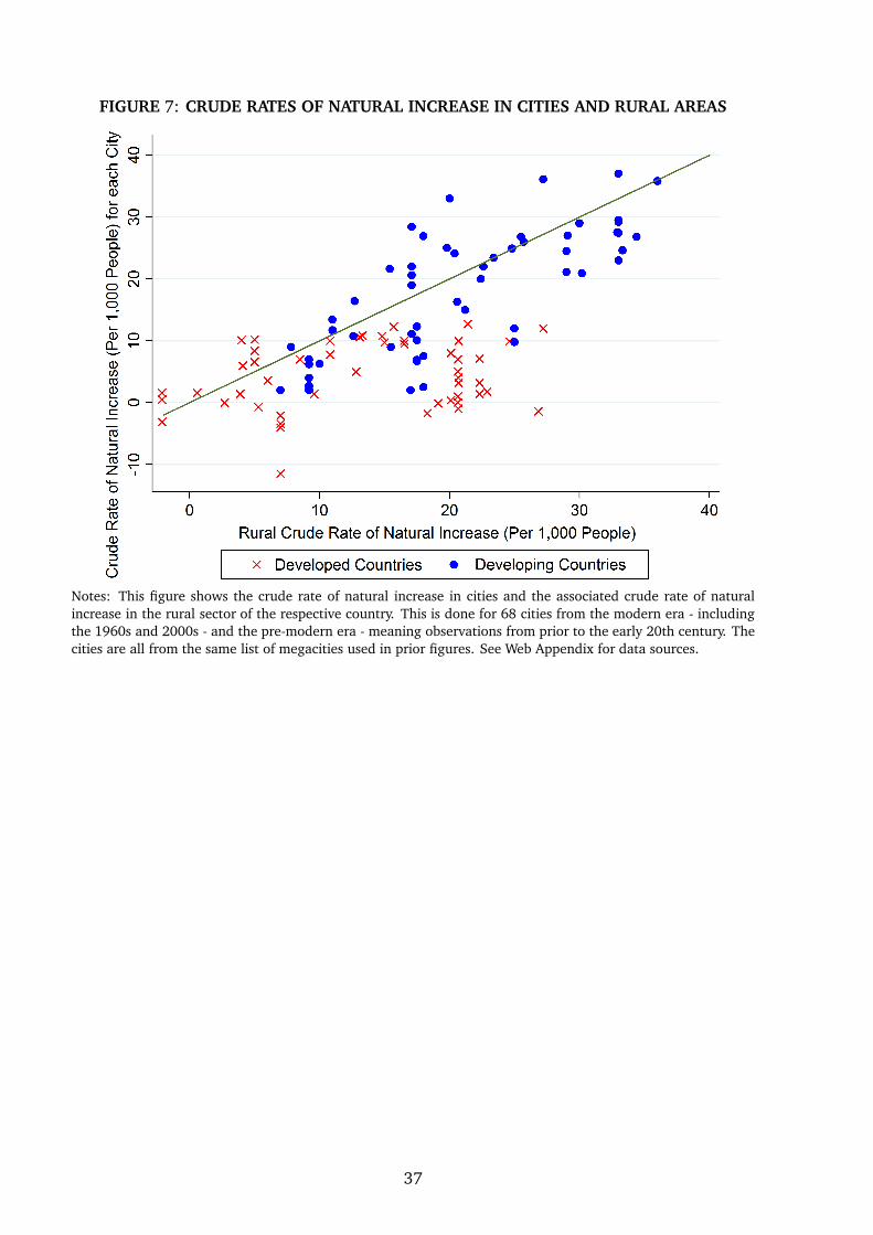
FIGURE 7: CRUDE RATES OF NATURAL INCREASE IN CITIES AND RURAL AREAS

Notes: This figure shows the crude rate of natural increase in cities and the associated crude rate of naturalincrease in the rural sector of the respective country. This is done for 68 cities from the modern era - includingthe 1960s and 2000s - and the pre-modern era - meaning observations from prior to the early 20th century. Thecities are all from the same list of megacities used in prior figures. See Web Appendix for data sources.

37

FIGURE 8: INCOME LEVEL AND CITY CRUDE RATES OF NATURAL INCREASE, 2000s

Notes: This graph shows the relationship between the crude rate of natural increase (per 1,000 people) for 38megacities in the 2000s and log per capita GDP (PPP, constant 2011 $) for the country of the megacity in 2000.See Web Appendix for data sources.

38

FIGURE 9: CRUDE RATES OF NATURAL INCREASE AND PROJECTED CITY GROWTH,2015-2030

Notes: This graph shows the relationship between the projected annual growth rate (%) in 2015-2030 and thecrude rate of natural increase (per 1,000 people) in the 2000s, for 38 megacities of Table 2. Data is missing forthe other megacities of the table. We use ? to obtain the projected growth rate of each city. These rates arebased on non-linear extrapolation given the rates of growth pre-2015, and are thus estimated independently ofthe rates of natural increase. See Web Appendix for data sources.

39

FIGURE 10: CRUDE RATES OF NATURAL INCREASE AND DEPENDENCY RATIO, 2000s

Notes: This graph shows the correlation between the dependency ratio (%) – the ratio of the population of 0-14y.o. plus above-65 y.o over the population of 15-64 y.o. – and the crude rate of natural increase (per 1,000people) for 37 megacities of Table 2 in the 2000s. See Web Appendix for data sources.

40

FIGURE 11: URBAN WAGE WITH INFORMAL SECTOR

Nu

wu

wuwinfu

N u N u

Notes: This figure shows the urban wage when there are two possible sectors of production. The formal sectordisplays both agglomeration (ρ > 0) and congestion (τ > 0) in production, which creates the inverted U-shapewith respect to urban population, Nu. The informal sector has neither agglomeration nor congestion (ρ = 0 andτ= 0), and so is invariant to Nu. The values Nu and Nu represent the cut-offs between which workers will chooseto work in the formal sector.

41

FIGURE 12: EQUILIBRIUM CITY SIZE WHEN w < winfu

Nu

wu/Auw

in fu

Au

wAu

Notes: This figure shows the equilibrium size of urban population when the Malthusian equilibrium wage (w)is smaller than the informal wage (winf

u ). With winfu > w, urban population size is always growing, and hence

there is no steady state value of Nu, and the urban sector grows without bound.

42

FIGURE 13: EQUILIBRIUM CITY SIZE WHEN w > winfu

Nu

wu/Auw

in fu

Au

wAu

N ∗∗u

N ∗u

Notes: This figure shows the equilibrium size of urban population when the Malthusian equilibrium wage (w) islarger than the informal wage (winf

u ). With wu > w, urban population size is growing, and with wu < w, urbanpopulation is falling. Given this, there is an unstable steady state at N ∗u , and a stable steady state at N ∗∗u .

43

TABLE 1: WORLD’S LARGEST MEGACITIES (MILLIONS), 1700-2015

Rank 1700 1900 1950 2015

1 Istanbul 0.7 London 6.5 New York 12.3 Tokyo 38.02 Tokyo 0.7 New York 4.2 Tokyo 11.3 Delhi 25.73 Beijing 0.7 Paris 3.3 London 8.4 Shanghai 23.74 London 0.6 Berlin 2.7 Paris 6.3 Sao Paulo 21.15 Paris 0.5 Chicago 1.7 Moscow 5.4 Mumbay 21.06 Ahmedabad 0.4 Vienna 1.7 Buenos Aires 5.1 Mexico 21.07 Osaka 0.4 Tokyo 1.5 Chicago 5.0 Beijing 20.48 Isfahan 0.4 St. Petersburg 1.4 Kolkata 4.5 Osaka 20.29 Kyoto 0.4 Manchester 1.4 Shanghai 4.3 Cairo 18.8

10 Hangzhou 0.3 Philadelphia 1.4 Osaka 4.1 New York 18.611 Amsterdam 0.2 Birmingham 1.2 Los Angeles 4.0 Dhaka 17.612 Naples 0.2 Moscow 1.1 Berlin 3.3 Karachi 16.613 Guangzhou 0.2 Beijing 1.1 Philadelphia 3.1 Buenos Aires 15.214 Aurangabad 0.2 Kolkata 1.1 Rio de Janeiro 3.0 Kolkata 14.915 Lisbon 0.2 Boston 1.1 St. Petersburg 2.9 Istanbul 14.216 Cairo 0.2 Glasgow 1.0 Mexico 2.9 Chongqing 13.317 Xian 0.2 Osaka 1.0 Mumbai 2.9 Lagos 13.118 Seoul 0.2 Liverpool 0.9 Detroit 2.8 Manila 12.919 Dacca 0.2 Istanbul 0.9 Boston 2.6 Rio de Janeiro 12.920 Ayutthaya 0.2 Hamburg 0.9 Cairo 2.5 Guangzhou 12.521 Venice 0.1 Buenos Aires 0.8 Tianjin 2.5 Los Angeles 12.322 Suzhou 0.1 Budapest 0.8 Manchester 2.4 Moscow 12.223 Nanking 0.1 Mumbay 0.8 Sao Paulo 2.3 Kinshasa 11.624 Rome 0.1 Ruhr 0.8 Birmingham 2.2 Tianjin 11.225 Smyrna 0.1 Rio de Janeiro 0.7 Shenyang 2.1 Paris 10.826 Srinagar 0.1 Warsaw 0.7 Roma 1.9 Shenzhen 10.727 Palermo 0.1 Tientsin 0.7 Milano 1.9 Jakarta 10.328 Moscow 0.1 Shanghai 0.6 San Francisco 1.9 London 10.329 Milan 0.1 Newcastle 0.6 Barcelona 1.8 Bangalore 10.130 Madrid 0.1 St. Louis 0.6 Glasgow 1.8 Lima 9.9

Sources: Chandler (1987) and United Nations (2014).

44

TABLE 2: PROJECTED ANNUAL GROWTH RATES FOR MEGACITIES (%), 2015-2030

Rank (1) Among Top 30 Cities in 2015 (2) Among All Cities ≥ 5 Millions in 2015

1 Lagos 4.2 Dar es Salaam 5.12 Kinshasa 3.7 Luanda 4.43 Dhaka 3.0 Lagos 4.24 Karachi 2.7 Kinshasa 3.75 Bangalore 2.6 Abidjan 3.26 Guangzhou 2.3 Khartoum 3.17 Delhi 2.3 Dhaka 3.08 Beijing 2.1 Surat 2.99 Jakarta 2.0 Karachi 2.7

10 Mumbay 1.9 Lahore 2.711 Tianjin 1.8 Suzhou 2.612 Chongqing 1.8 Bangalore 2.613 Cairo 1.8 Baghdad 2.614 Manila 1.8 Ahmadabad 2.415 Shanghai 1.8 Hyderabad 2.416 Kolkata 1.7 Pune 2.317 Lima 1.4 Guangzhou 2.318 Shenzhen 1.1 Chennai 2.319 Istanbul 1.1 Delhi 2.320 Mexico 0.9 Ho Chi Minh 2.321 Buenos Aires 0.7 Hangzhou 2.222 London 0.7 Kuala Lumpur 2.223 Sao Paulo 0.7 Beijing 2.124 Rio de Janeiro 0.6 Yangon 2.125 Paris 0.6 Jakarta 2.026 Los Angeles 0.5 Chengdu 2.027 New York 0.5 Nanjing 2.028 Moscow 0.0 Mumbai 1.929 Osaka -0.1 Xian 1.930 Tokyo -0.1 Cairo 1.8

Notes: This table shows the fastest-growing megacities among: (1) the top 30 cities in 2015, and (2) the citiesof at least 5 million inhabitants in 2015. Sources: Chandler (1987) and United Nations (2014).

45