malware analysis using pro le hidden markov models and ... · malware analysis using pro le hidden...
TRANSCRIPT

Malware Analysis using Profile Hidden Markov Models
and Intrusion Detection in a stream learning setting
A Thesis
Submitted For the Degree of
Master of Science (Engineering)
in the Faculty of Engineering
by
Saradha R
Supercomputer Education and Research Centre
Indian Institute of Science
BANGALORE – 560 012
May 2014

i
c©Saradha R
May 2014
All rights reserved

TO
Bhagawan Sri Ramana Maharishi and His grace

Acknowledgements
First of all I would like to thank my Research advisor Professor N.Balakrishnan for
all his support and advice. He has encouraged and motivated me to learn about and
work on some interesting problems in the area of computer security. He is been very
instrumental in my growth as a researcher and gave the right perspective to view the
problems, in very important junctures. He gave me and all his students the great op-
portunity to interact with and learn from some of the greatest minds in the country. I
shall always hold the lessons I learnt from him about striving for excellence and results
of hardwork, very close to my heart. He and Mrs. Jyothi Balakrishnan have been the
pillar of support, during many tough times. I shall always remain indebted to him
for all his kindness and guidance. I consider myself very privileged to be part of the
Information Systems Lab in SERC, IISc.
Next I would like to thank the Chairman of Supercomputer Education and Research
Centre, Prof. Govindarajan for his support and encouragement. The resources and
facilities in SERC were always available for the students doing research. I also whole-
heartedly thank my colleagues and friends in my lab., Bharath, Naimisha, Sudheep,
Indira Ma’m, Prashant Kulkarni, Prashant Sharma, Nikhil Koul, Pritam padhy, Sachin
Singh and Venkat Padhy for their unwavering support and help. Work gave me so
much joy, when done in the company of such motivated and cheerful people. I wish to
thank all my teachers who have been a great source of inspiration; especially Prof. P
A Shastry, Prof. Vittal Rao, Prof. Joy Kuri, Prof. Veni Madhavan and Prof. Mathew
i

ii
Jacob.
I also want to thank my friends Arun, Raman, Hariprasad, LakshmiNarasimhan, LP,
Madhavan and the gang.Special thanks to my music Guru Deepak Paramashivam.
They have motivated me so deeply to excel in whatever I do and have taught me
the importance of staying humble and simple. I also wish to thank wholeheartedly,
Ms.Nagarathna, Mrs Swarnalatha Ramesh and Mr.RaviKumar for their support and
help, throughout. I thank my husband Dev for his unwavering support. And I thank
all my friends, employees and colleagues at IISc for making it a memorable time of my
life.
Publications based on this Thesis
1. Ravi S., Balakrishnan N. and Venkatesh B. (2013), Behavior-based Malware Anal-
ysis using Profile Hidden Markov Models. In Proceedings of the 10th International
Conference on Security and Cryptography, pages 195-206. DOI: 10.5220/0004528201950206
2. Saradha R., Nikhil K., Balakrishnan N. (2011) Behavior-based malware classifi-
cation using Profile Hidden Markov Models. Poster accepted at the Women in
Machine Learning Workshop (NIPS 2011), Granada, Spain.
iii
Abstract
In the last decade, a lot of machine learning and data mining based approaches have
been used in the areas of intrusion detection, malware detection and classification and
also traffic analysis. In the area of malware analysis, static binary analysis techniques
have become increasingly difficult with the code obfuscation methods and code packing
employed when writing the malware. The behavior-based analysis techniques are being
used in large malware analysis systems because of this reason. In prior art, a number
of clustering and classification techniques have been used to classify the malwares into
families and to also identify new malware families, from the behavior reports. In this
thesis, we have analysed in detail about the use of Profile Hidden Markov models for
the problem of malware classification and clustering. The advantage of building accu-
rate models with limited examples is very helpful in early detection and modeling of
malware families.
The thesis also revisits the learning setting of an Intrusion Detection System that
employs machine learning for identifying attacks and normal traffic. It substantiates
the suitability of incremental learning setting(or stream based learning setting) for the
problem of learning attack patterns in IDS, when large volume of data arrive in a stream.
Related to the above problem, an elaborate survey of the IDS that use data mining
and machine learning was done. Experimental evaluation and comparison show that in
terms of speed and accuracy, the stream based algorithms perform very well as large
iv

v
volumes of data are presented for classification as attack or non-attack patterns. The
possibilities for using stream algorithms in different problems in security is elucidated
in conclusion.

Contents
Acknowledgements i
Publications based on this Thesis iii
Abstract iv
Keywords x
Notation and Abbreviations xi
1 Introduction 11.1 Types of cyber attacks . . . . . . . . . . . . . . . . . . . . . . . . . . . . . . . . . . . . . 11.2 Role of malware in Cyber attacks . . . . . . . . . . . . . . . . . . . . . . . . . . . . . . . 2
1.2.1 Viruses . . . . . . . . . . . . . . . . . . . . . . . . . . . . . . . . . . . . . . . . . 31.2.2 Worms . . . . . . . . . . . . . . . . . . . . . . . . . . . . . . . . . . . . . . . . . . 31.2.3 Trojan horses . . . . . . . . . . . . . . . . . . . . . . . . . . . . . . . . . . . . . . 31.2.4 Spyware . . . . . . . . . . . . . . . . . . . . . . . . . . . . . . . . . . . . . . . . . 41.2.5 Botnets . . . . . . . . . . . . . . . . . . . . . . . . . . . . . . . . . . . . . . . . . 4
1.3 Malware menace in recent times . . . . . . . . . . . . . . . . . . . . . . . . . . . . . . . 51.4 Defense mechanisms . . . . . . . . . . . . . . . . . . . . . . . . . . . . . . . . . . . . . . 71.5 Malware Analysis . . . . . . . . . . . . . . . . . . . . . . . . . . . . . . . . . . . . . . . 9
1.5.1 Static malware analysis . . . . . . . . . . . . . . . . . . . . . . . . . . . . . . . . 101.5.2 Signature-based techniques . . . . . . . . . . . . . . . . . . . . . . . . . . . . . . 111.5.3 Problems in static analysis . . . . . . . . . . . . . . . . . . . . . . . . . . . . . . 111.5.4 Polymorphic malware . . . . . . . . . . . . . . . . . . . . . . . . . . . . . . . . . 121.5.5 Metamorphic malware . . . . . . . . . . . . . . . . . . . . . . . . . . . . . . . . . 12
1.6 Code obfuscation techniques . . . . . . . . . . . . . . . . . . . . . . . . . . . . . . . . . . 121.7 Dynamic malware analysis . . . . . . . . . . . . . . . . . . . . . . . . . . . . . . . . . . . 141.8 Unsupervised and Supervised models on Dynamic analysis reports . . . . . . . . . . . . 141.9 Related work in Dynamic analysis . . . . . . . . . . . . . . . . . . . . . . . . . . . . . . 151.10 Motivation and Problem statement . . . . . . . . . . . . . . . . . . . . . . . . . . . . . . 181.11 Organisation of the thesis . . . . . . . . . . . . . . . . . . . . . . . . . . . . . . . . . . . 20
2 Mathematical basis for chosen approach and Evaluation Metrics 222.1 Introduction . . . . . . . . . . . . . . . . . . . . . . . . . . . . . . . . . . . . . . . . . . . 222.2 Profile Hidden Markov Models . . . . . . . . . . . . . . . . . . . . . . . . . . . . . . . . 22
2.2.1 Hidden Markov Models . . . . . . . . . . . . . . . . . . . . . . . . . . . . . . . . 232.2.2 Profile Hidden Markov Model in detail . . . . . . . . . . . . . . . . . . . . . . . . 24
2.3 Classification Evaluation Metrics . . . . . . . . . . . . . . . . . . . . . . . . . . . . . . . 272.3.1 Precision . . . . . . . . . . . . . . . . . . . . . . . . . . . . . . . . . . . . . . . . 282.3.2 Recall . . . . . . . . . . . . . . . . . . . . . . . . . . . . . . . . . . . . . . . . . . 282.3.3 F- Score . . . . . . . . . . . . . . . . . . . . . . . . . . . . . . . . . . . . . . . . . 282.3.4 Confusion Matrix . . . . . . . . . . . . . . . . . . . . . . . . . . . . . . . . . . . . 282.3.5 Accuracy . . . . . . . . . . . . . . . . . . . . . . . . . . . . . . . . . . . . . . . . 292.3.6 Kappa statistic . . . . . . . . . . . . . . . . . . . . . . . . . . . . . . . . . . . . . 29
2.4 Clustering Comparison Metrics . . . . . . . . . . . . . . . . . . . . . . . . . . . . . . . . 292.4.1 Precision and Recall . . . . . . . . . . . . . . . . . . . . . . . . . . . . . . . . . . 30
vi

CONTENTS vii
3 Malware Classification and Clustering using PHMM based approach 313.1 Initial Experiments . . . . . . . . . . . . . . . . . . . . . . . . . . . . . . . . . . . . . . . 313.2 Methodology . . . . . . . . . . . . . . . . . . . . . . . . . . . . . . . . . . . . . . . . . . 333.3 Results . . . . . . . . . . . . . . . . . . . . . . . . . . . . . . . . . . . . . . . . . . . . . . 363.4 Closer look at malware analysis . . . . . . . . . . . . . . . . . . . . . . . . . . . . . . . . 383.5 Challenges in practice . . . . . . . . . . . . . . . . . . . . . . . . . . . . . . . . . . . . . 393.6 Detailed Experiments . . . . . . . . . . . . . . . . . . . . . . . . . . . . . . . . . . . . . 40
3.6.1 Encoding the behaviour reports . . . . . . . . . . . . . . . . . . . . . . . . . . . . 413.6.2 Incremental setting for the detailed experiments . . . . . . . . . . . . . . . . . . 41
3.7 What is Phylogeny? . . . . . . . . . . . . . . . . . . . . . . . . . . . . . . . . . . . . . . 433.7.1 Malware Phylogeny . . . . . . . . . . . . . . . . . . . . . . . . . . . . . . . . . . 43
3.8 Analysis of the results . . . . . . . . . . . . . . . . . . . . . . . . . . . . . . . . . . . . . 45
4 Intrustion Detection in a Data Stream 494.1 Brief Introduction to machine learning . . . . . . . . . . . . . . . . . . . . . . . . . . . . 504.2 Stream-based learning paradigm . . . . . . . . . . . . . . . . . . . . . . . . . . . . . . . 514.3 Intrusion detection systems employing machine learning - A survey . . . . . . . . . . . . 514.4 Commonly used datasets for validation of an IDS . . . . . . . . . . . . . . . . . . . . . . 54
4.4.1 DARPA 1999 Dataset for Intrusion Detection . . . . . . . . . . . . . . . . . . . . 544.4.2 The KDD Cup 1999 Dataset . . . . . . . . . . . . . . . . . . . . . . . . . . . . . 55
4.5 Stream based learning algorithm . . . . . . . . . . . . . . . . . . . . . . . . . . . . . . . 574.6 Hoeffding Trees . . . . . . . . . . . . . . . . . . . . . . . . . . . . . . . . . . . . . . . . . 58
4.6.1 Special properties of the Hoeffding trees . . . . . . . . . . . . . . . . . . . . . . . 594.7 Online learning . . . . . . . . . . . . . . . . . . . . . . . . . . . . . . . . . . . . . . . . . 60
4.7.1 Online Prediction from Experts . . . . . . . . . . . . . . . . . . . . . . . . . . . . 614.7.2 Weighted Majority algorithm . . . . . . . . . . . . . . . . . . . . . . . . . . . . . 61
4.8 Experiments and Results . . . . . . . . . . . . . . . . . . . . . . . . . . . . . . . . . . . . 62
5 Conclusion 675.1 Contribution of the thesis . . . . . . . . . . . . . . . . . . . . . . . . . . . . . . . . . . . 675.2 Directions for future work . . . . . . . . . . . . . . . . . . . . . . . . . . . . . . . . . . . 68
References 71

List of Tables
1.1 Samples of code obfuscation . . . . . . . . . . . . . . . . . . . . . . . . . . . . . . . . . . 13
3.1 Malware Clustering Comparision of PHMM based method and N-grams method . . . . 43
4.1 Accuracies and Kappa-statistic for various Stream learning algorithms on the KDD Cup99 dataset . . . . . . . . . . . . . . . . . . . . . . . . . . . . . . . . . . . . . . . . . . . . 63
viii

List of Figures
1.1 Total malware count over Years . . . . . . . . . . . . . . . . . . . . . . . . . . . . . . . . 61.2 New malware count over Years . . . . . . . . . . . . . . . . . . . . . . . . . . . . . . . . 61.3 Example of code reordering . . . . . . . . . . . . . . . . . . . . . . . . . . . . . . . . . . 13
2.1 The transition structure of a profile HMM. For example, from an insert state (diamond),we can go to the next delete state (circle), continue in the insert state (self loop) orgo to the next match state (rectangle). Note that while multiple sequential deletionsare possible by following the circle states, each with a different probability, multiplesequential insertions are only possible with the same probability[4] . . . . . . . . . . . . 25
2.2 A sample MSA file for EJIK Malware Sequences . . . . . . . . . . . . . . . . . . . . . . 26
3.1 The different malware families and the number of files in each, as in Malheur referencedataset[19] . . . . . . . . . . . . . . . . . . . . . . . . . . . . . . . . . . . . . . . . . . . . 32
3.2 Sample of MIST representation of a portion of CWSandbox report[3] (a) and (b) . . . . 353.3 (a) Histogram of accuracy and 3.3(b)Histogram of F-Scores . . . . . . . . . . . . . . . . 373.4 Confusion matrix for malware classification . . . . . . . . . . . . . . . . . . . . . . . . . 383.5 Phylogenetic tree for Virut and Kies . . . . . . . . . . . . . . . . . . . . . . . . . . . . . 463.6 Phylogenetic tree for Palevo and Buzus . . . . . . . . . . . . . . . . . . . . . . . . . . . 473.7 Clustering Results - Top 15 clusters . . . . . . . . . . . . . . . . . . . . . . . . . . . . . 48
4.1 Broad Classification of machine learning . . . . . . . . . . . . . . . . . . . . . . . . . . 524.2 Accuracy Comparison Graph . . . . . . . . . . . . . . . . . . . . . . . . . . . . . . . . . 654.3 Kappa Comparison Graph) . . . . . . . . . . . . . . . . . . . . . . . . . . . . . . . . . . 654.4 Evaluation Time (in CPU secs) . . . . . . . . . . . . . . . . . . . . . . . . . . . . . . . . 66
ix

Keywords
Malware analysis, Malware classification and clustering, Polymorphic viruses, Dynamic
malware analysis, Profile Hidden Markov Models, Multiple Sequence Alignment, Huff-
man encoding, Phylogenetic trees, Intrusion Detection Systems, Misuse Detection,
Anomaly Detection, Data mining, Batch learning, Online learning, Stream-based learn-
ing, Hoeffding trees, Weighted-Majority algorithm
x

Notation and Abbreviations
• IDS - Intrustion Detection System
• PHMM - Profile Hidden Markov Model
• IPS - Intrusion Prevention System
• MOA - Massive Online Analysis Framework
• HMM - Hidden Markov Model
• KDD - Knowledge Discovery in Databases
• DoS - Denial Of Service
• DoD - Department Of Defense (USA)
• F-Score - Figure of merit score
• TCP - Transmission Control Protocol
• IP - Internet Protocol
• Σ - The alphabet of symbols in a Hidden Markov Model
• Z - The set of hidden states in a Hidden Markov Model
• E|Z|x|Σ| - The emission probability matrix in a Hidden Markov Model
• A|Z|x|Z| - The state transmission matrix in a Hidden Markov Model
• π - The initial state distribution in a Hidden Markov Model
xi

LIST OF FIGURES xii
• X - The instance space in an online learning setting
• xt - The data instance in round t of online learning algorithm
• N - Dimensionality of the Instance space
• yt - True label of the data instance in round t of online learning algorithm
• yt - Predicted label of the data instance in round t
• `(yt, yt) - Loss function defined over true and predicted labels

Chapter 1
Introduction
A cyber attack system is any kind of offensive system used by individuals or large or-
ganizations that targets infrastructures, computer networks and information systems,
and other devices in various malicious ways. The threats or attacks usually originate
from an anonymous source that either steals, changes, or completely destroys particular
target by hacking into a vulnerable part of the system. Cyber-attacks have become in-
creasingly sophisticated and dangerous and a preferred method of attacks against large
entities, by attackers. Cyber-war or cyber-terrorism is synonymous with cyber attacks
and exploits three main factors for terrorising people that further impairs tourism, de-
velopment and smooth functioning of governments and other infrastructure in a country
or a large business corporations. These factors are fear about security of lives, large
scale economic loss that causes negative publicity about a corporation or government
and vulnerability of government systems and infrastructure that raises questions about
the integrity and authenticity of data that is published in them.
1.1 Types of cyber attacks
We can list down the different kinds of cyber attacks in an increasing order of sophisti-
cation and complexity of the attack itself. The order is also chronological in some ways
since the attacks have become more sophisticated with time in order to stay ahead of the
1
Chapter 1. Introduction 2
security systems that are used in the networks and on individual systems. The initial
attacks on computers were more social engineering attacks that were not very compli-
cated and were aimed at individual hosts. The network sniffers, packet sniffing and
session hijacking attacks came next, with the advent of internetworking. Automated
probes and scans that came next, do reconnaissance following which widespread attacks
such as the distributed denial of service type attacks were executed. Viruses that took
advantage on the vulnerability in a software just by looking at compiled code came into
picture. The more sophisticated viruses that spread through emails and widespread
trojans came alongside. Anti-forensic malware and worms that escape the security sys-
tems by using encryption and code packing, are very rampant in recent times. So are
the increasingly sophisticated network of compromised hosts, called botnets. Botnets
have command and control capability within its own network and is capable of doing
extremely large-spread attacks in the scale of internet.[58]
1.2 Role of malware in Cyber attacks
In all these different techniques from the early times to now, one component of the
attack architecture necessarily needs to be detected and mitigated from spreading itself.
These are the malicious executable files or the malware, that do the bulk of the intrusive
activities on a system and that spreads itself across the hosts in a network.
Malicious software (malware) is defined as software performing actions intended by an
attacker, mostly with malicious intentions of stealing information, identity or other
resources in the computing systems. The different types of malware include worms,
viruses, Trojan horses, bots, spyware and adware. They all exhibit different sort of
malicious behaviour on the target systems and it is essential to prevent their activity
and further proliferation in the network using different methods.

Chapter 1. Introduction 3
1.2.1 Viruses
A virus is a program that copies itself and infects a host, spreading from one file to
another, and then from one host to another, when the files are copied or shared. The
viruses usually attach themselves mostly to executable files and sometimes with master
boot record, autorun scripts, MS Office Macros or even other types of files.The theoret-
ical preliminary work on computer viruses goes back as far as 1949. John von Neumann
(1903-1957) developed the theory of self-reproducing automatons. The function of a
virus is to essentially destroy or corrupt files on the infected hosts. It was in 1984
that Fred Cohen introduced the implementation of computer virus and exhibited its
capabilities on a unix machine.[59]. The ”Brain” virus that infected the boot sector of
the DOS operating system was released in 1986.
1.2.2 Worms
Computer worms send copies of themselves to other hosts in the network, usually
through security vulnerabilities in the operating systems or the software. They spread
automatically most often without any user intervention.The worms spread very rapidly
over the network affecting many hosts in their path. They comprise the majority
of the malware and are often mistakenly called viruses. Some of the most famous
worms include the ILOVEYOU worm, transmitted as an email attachment, that cost
businesses upwards of 5.5 billion dollars in damage. The Code Red worm defaced
359,000 web sites[60]. SQL Slammer had slowed down the entire internet for a brief
period of time and the famous Blaster worm would force the host computer to reboot
repeatedly.
1.2.3 Trojan horses
Trojan horses are applications that appear to be doing something innocuous, but se-
cretly have malicious code that has intrusive behavior. In many cases, trojans usually

Chapter 1. Introduction 4
create a backdoor that allows the host to be controlled remotely either directly or as
part of a botneta network of computers also infected with a trojan or other malicious
software. The major difference between a virus and a trojan is that trojans do not
replicate themselves. They are usually installed by an unsuspecting user. PC Writer
was the first trojan horse pogram that came out in 1986. It pretended to be like a
legitimate installable for the shareware PC Writer Word processing program. But on
execution the trojan horse would start and delete all data on the hard disk and format
the drive.
1.2.4 Spyware
Spyware is any software installed on a host which collects your information without
the consent or knowledge of the user, and sends that information back to its author.
This could include keylogging to learn about passwords,and other sensitive information.
The spyware starts installing unwanted software and toolbars in the browsers without
the knowledge or consent from the user. Many people have spyware running in their
systems without even realizing it, but generally those that have one spyware application
installed also have a dozen more. The sign for its presence is that the computer becomes
very slow and many unknown software are usually automatically installed.
1.2.5 Botnets
Botnets are networks of compromised hosts which can be remotely controlled by an
attacker who is usually referred to as the botmaster or the bot-herder. A bot is typically
connected to the Internet, and mostly affected by a malware akin to a trojan horse. The
botmaster can control each bot remotely over the network. It can instruct the bots to
do malware update, send spam emails and steal information. The operation of the bots
are controlled using a command and control (C2C) channel, which can be centralized
or peer-to-peer[58]. The topology of the command and control channel determines the

Chapter 1. Introduction 5
efficiency and resilience of the botnet. The botnet detection is an active area of research
due to the inherent complexity and scale of the problem.
1.3 Malware menace in recent times
The proliferation of malware in recent times is obvious from the statistics gathered,
over the years.From the data gathered from an independent IT security company AV-
Test, we see that the total number of malware on the internet has reached about 100
million in the year 2012. Over 30 million new malware instances have appeared in the
year 2012 alone, which is twice the number of unseen malware that were introduced in
the previous year. The plots in Fig. 1.1 and 1.2 show the total and the new types of
malware that were seen over the years.
A range of malicious software/systems, ranging from classic computer viruses to In-
ternet worms and bot networks, target computer systems linked to a private networks or
the Internet. Proliferation of this threat is driven by a criminal industry which system-
atically comprises networked hosts for illegal purposes, such as gathering of confidential
data, distribution of spam messages, and misuse of information for economic gains etc.
According to McAfee, MyDoom is a massive spam-mailing malware that caused the
most economic damage of all time, an estimated $38 billion. Conficker was a botnet
employed for password stealing and it caused an estimated $9.1 billion damage. Un-
fortunately, the rising numbers and high diversity of malware render classic security
techniques, such as anti-virus scanners, not very useful and have resulted in millions of
hosts in the Internet infected with malicious software (Microsoft, 2009; Symantec, 2009)
From the above discussion, it is seen clearly that a huge task of improving the detec-
tion capability and methodology on the host lies on the antivirus products. They are

Chapter 1. Introduction 6
Figure 1.1: Total malware count over Years
Figure 1.2: New malware count over Years

Chapter 1. Introduction 7
constantly challenged by the malware which make use of known or unknown vulnera-
bilities in the software or the network systems to come up with new kinds of attacking
and hiding mechanisms. The antivirus companies employ many ways of creating the
database of known attack vectors to detect known attacks. One of them is to collect
any suspicious looking files or binaries (or those that were known to cause problems)
that are identified by the end users or another system, and then analyse them. This
process, called malware analysis, encompasses the steps of malware detection and mal-
ware classification. These need not be separate steps in the whole process, though in
some practical implementations they may be.
1.4 Defense mechanisms
In this section, we review the detection and prevention solutions for cyber attacks in
general and malware in particular. When we talk about security solutions it is obvious
to start with defining an Intrusion Detection System. An Intrusion Detection System
can be a device or a software that monitors a network or a system, for malicious
activities and generates a reports for a management station[47]. They usually detect
the intrusion that have already occurred or that which are in progress. The most early
systems in 60s and 70s involved looking for suspicious or unusual events in system audit
logs. The amount or granularity of audit logs that are analysed is a tradeoff between
overhead and effectiveness. The host based IDS refers to a system that is deployed
on individual hosts; This is usually an agent program that does event correlation, log
analysis, integrity checking, policy enforcement etc. on a system level. The Anti-
virus solutions are a type of HIDS that monitor the dynamic behavior of the host
system. They monitor every user and system activity and raise alarm on any security
policy violation at user and system level. The Anti-virus software products study and
analyse the malware and come up with unique patterns or signatures to identify the
Chapter 1. Introduction 8
different types of malware. This is necessary since the cleanup, quarantine and removal
procedures for each kind of malware is different from one another.
Everyday the anti-virus companies receive tens of thousands of instances of possi-
ble malicious files that have to be analysed, in a quick and efficient way. For this the
signature-based malware detection techniques are widely used owing to their speed and
effectiveness. But they may not give a complete coverage for all possible attacks, since
the malware toolkits generate polymorphic and metamorphic variants of viruses and
worms that easily outsmart the signature based systems. After analysis, the binaries
are given labels and the signatures are extracted for newly seen variants and stored in
the virus database.Throughout the thesis, we define malware analysis as classifying or
clustering a malware to a particular family or group and do not address the problem
of malware detection alone. The problem and the existing solutions for solving it are
explained in detail in the coming sections.
We now will look at the role of IDS in detection of previously unseen zero-day attacks.
Apart from the Host-based IDS discussed before the other class of IDS that is used
to monitor the activities and incidents going in a network form the class of Network
Intrusion Detection Systems. Several rule-based and statistical methods have been
employed in the existing NIDS. Some IDS use deep packet inspection in the network
traffic data while some methods use header information in the packets or do sifting of
the traffic data at various level of granularity, to look for abnormal patterns. The traffic
data can be voluminous and sampling the data to look for patterns, especially for rare
and previously unseen events such as a virus attack can be challenging task. Also the
attacks can be crafted in such as way as to exhaust the resources that are used in the
IDS platform.

Chapter 1. Introduction 9
The other main classification of IDS is done based on the choice of modeling the
attack and the non-attack or benign data.There are misuse- detection systems or the
signature-based detection systems that model the patterns of previously known attacks.
These could be hand-crafted signatures or even rules learnt by a system, that charac-
terised a known attack. These systems are fast in detecting known attacks but are very
weak in detecting zero-day attacks. Also the speed of these systems tend to be slower
as the database of signature grows and most often than not, the attacks are detected
after they occur only. The other class of IDS is the anomaly detection systems, that
models the normal non-malicious behavior of the system and ags any deviation from
that as abnormal. They are very effective in identifying new unseen attacks, but suffer
from the problem of high false-positive rates. Also the environment is so dynamic that
the very definition of what is normal or abnormal data itself changes over time, posing
more challenges in modeling the system. The Intrusion Detection Systems that make
use of statistical features in the traffic patterns and/or payload data, have the inherent
problem when it comes to relearning the model. An efficient strategy for relearning
becomes very important and there are very few prior work that address this. Also the
machine learning system itself can become vulnerable to manipulative training data
injected by the hackers in order to mislead the system into modeling malicious code
as non malicious. Thus the security of a batch-trained model itself becomes a serious
concern [62].
1.5 Malware Analysis
The malware analysis that Anti-virus companies do, can be classified broadly into two
categories; the static analysis techniques and the dynamic analysis techniques. The
static techniques involve looking into the binaries directly or the reverse engineering

Chapter 1. Introduction 10
the code for patterns in the same. The dynamic analysis techniques involve captur-
ing the behavior of the malware sample by executing it in a sandboxed environment
or by program analysis methods and then use that for extracting patterns for each
family of virus. Examples for these are systems like Anubis, [21] and CWSandbox.
Of late static binary analysis techniques are becoming increasingly difficult with the
code obfuscation methods and code packing employed when writing the malware. The
behavior-based analysis techniques are preferred in more sophisticated malware anal-
ysis systems because of this reason. In previous works, a number of clustering and
classification techniques from machine learning have been used to classify the malware
into families and to also identify new malware families, from the behavior reports. In
our experiments, we propose to use the Prole Hidden Markov Model[6] to classify the
malware les into families or groups based on their behavior on the host system. We
have looked at the challenges involving analysis of a large number of malware infected
les, and show an extensive evaluation of our method in the following chapter.
1.5.1 Static malware analysis
Signature based detection is used to identify a virus or family of viruses. A signature
based detector needs to update its list of signatures more often. Since the signature of
a new virus would not be available in the database, it is not possible to detect it as a
new virus. Detectors sometimes look into heuristics instead of relying on signatures.
However, signatures form a formidable percentage in the detection process. Signature
detection is fast and simple. Polymorphic and metamorphic viruses cannot be contained
using signature detection. Metamorphic malware use a combination of various code
obfuscation techniques. Storing signatures of each variant of a malware is practically
not feasible since it increases the dictionary of the detector with unnecessary signatures.

Chapter 1. Introduction 11
1.5.2 Signature-based techniques
Signature-based detection provides undeniable advantages for operational use. It uses
optimized pattern matching algorithms with controlled complexity and very low false
positive rates. Unfortunately, form-based detection proves completely overwhelmed by
the quick evolution of the viral attacks. The bottleneck in the detection process lies
in the signature generation and the distribution process following the discovery of new
malware. The signature generation is often a manual process requiring a tight code
analysis that is extremely time consuming. Once generated, it must be distributed to
the potential targets. In the best cases, this distribution is automatic but if this update
is manually triggered by the user, it can still take days. In a context where worms such
as Sapphire are able to infect more than 90% of the vulnerable machines in less than
10 min, attacks and protection do not act on the same time scale.
1.5.3 Problems in static analysis
In the past few years the number of observed malware samples has increased dramati-
cally. This is due to the fact that attackers started to morph malware samples in order
to avoid detection by syntactic signatures. McAfee, a manufacturer of malware detec-
tion products, reported that 1.7 million out of 2.8 million malware samples collected
in 2007 are polymorphic variants of other samples. As a consequence a huge number
of signatures need to be created and distributed by anti-malware companies. These
have to be processed by detection products at the users system, leading to degradation
of the systems performance. Malware behavior families can address this problem. So,
all polymorphic variants of a particular sample are treated as members of the same
malware behavior family. For this, we need an automatic method for appropriately
grouping samples into respective behavior families.

Chapter 1. Introduction 12
1.5.4 Polymorphic malware
The variants produced by polymorphic malware constantly change. This is done by file-
name changes, compression, encrypting with variable keys, etc. Polymorphic malware
produce different variants of itself while keeping the inherent functionality as same.
This is achieved through polymorphic code, which is core to a polymorphic malware.
1.5.5 Metamorphic malware
Metamorphic malware represent the next class of virus that can create an entirely
new variant after reproduction. Unlike, polymorphic malware, metamorphic malware
contain a morphing engine. The morphing engine is responsible for obfuscating malware
completely. The body of a metamorphic malware can be broadly divided into two
parts - namely Morphing engine and Malicious code Metamorphic malwares use code
obfuscation techniques as opposed to encryption used by polymorphic viruses.
1.6 Code obfuscation techniques
Code obfuscation is a technique of deliberately making code hard to understand and
read. The resulting code after obfuscation has the same functionality. There are a
variety of code obfuscation techniques namely Garbage Code Insertion, Register Re-
naming, Subroutine Permutation, Code reordering and Equivalent code substitution
that are heavily used in the metamorphic virus generation toolkits. The Table 1.1 is
an example of equivalent code substitution and garbage code insertion. The following
figure shows an example of code re-ordering that is done using unconditional jump in-
structions. Of all these methods the subroutine permutation is little easier to detect
using signature-based technique since there is no actual modification of the instructions,
as such.

Chapter 1. Introduction 13
Table 1.1: Samples of code obfuscationOriginal
¯Obfuscated Version 1
¯
call DeltaDelta: pop ebp
sub ebp, offset Delta
call DeltaDelta: sub dword ptr[esp], offset Delta
pop eaxmov ebp, eax
Original¯
Obfuscated Version 2¯
call DeltaDelta: pop ebp
sub ebp, offset Delta
add ecx,0031751B ; junkcall Delta
Delta: sub dword ptr[esp], offset Deltasub ebx,00000909 ; junk
mov edx,[esp]xchg ecx,eax ; junkadd esp,00000004
and ecx,00005E44 ; junkxchg edx,ebp
Figure 1.3: Example of code reordering

Chapter 1. Introduction 14
1.7 Dynamic malware analysis
Automated, dynamic malware analysis systems work by monitoring a programs execu-
tion and generating an analysis report summarizing the behavior of the program. These
analysis reports typically cover file activities (e.g., what files were created), Windows
registry activities (e.g., what registry values were set), network activities (e.g., what
files were downloaded, what exploit were sent over the wire), process activities such as
when a process was created or terminated and Windows service activities such as when
the service was installed or started in the system etc. Several of them are publicly
available on the Internet (Anubis, CWSandbox , Joebox , Norman Sandbox ). The
main thing to note about dynamic analysis systems is that they execute the binary
for a limited amount of time. Since malicious programs do not reveal their behavior
when only executed for several seconds, dynamic systems are required to monitor the
binarys execution for a longer time. Thus dynamic analysis is resource-intensive in
terms of necessary hardware and time. There is also the problem of multiple paths in
the execution sequence and analysing all of them may not be possible in a sandbox
environment.
1.8 Unsupervised and Supervised models on Dynamic analysis
reports
Machine learning approaches like classification and clustering of malware have been
proposed on reports generated from dynamic analysis. Models are built for malware
families whose labels are available and used for predicting the malware labels for newly
seen sample reports. These models can generalise well, depending on the learning
algorithm and the sample training data from which they were built. The state-of-
the-art malware analysis systems perform a step of classification followed by a step of
clustering. In the next section, a detailed review of these systems and their performance

Chapter 1. Introduction 15
is presented.
1.9 Related work in Dynamic analysis
In this section, we will look at some of the related work done in the behavior-based
malware analysis and classification. In malware analysis problem, there is not just one
standard dataset in all previous research. Most malware datasets are collected over a
certain periods of time using a honeynet setup and they comprise PE executables, aimed
to attack Window based systems. The dynamic analysis techniques gained prominence
because of the limitations in the static analysis techniques [14].Moser et al proposed a
method where the normal model of programs were modeled using sequences of six sys-
tem calls and any deviations from this was flagged as anomaly or a security threat.This
was one of the first approaches of using behavior to differentiate malware from benign
programs.
Bailey et al[15] tracked more abstract features like system state changes rather than
system call sequences for malware classification. The clustering method they have used
looks at overall system state and generates a behavioral fingerprint for each malware
analysed. This is one of the earlier works that addressed the issue of anti-virus label-
ing inconsistencies.The Normalised Compression Distance is computed for every pair
of malware samples and a simple hierarchical clustering method (using single linkage)
was done on a dataset of malware collected in a sandbox system running Windows XP.
There were 3360 malware that were analysed and resulting clustering had 403 clusters.
In comparison with labellings by popular anti-virus systems like Symantec, McAfee,
FProt and ClamAV, the behavior based method gave much better detection accuracy
of 91% and consistent labeling for a given behavior profile. The authors however men-
tion that behavior profiles can be looked at a finer level (rather than state changes
alone) with modern system audit and trace systems such as CWSandbox, for better

Chapter 1. Introduction 16
performance. Also the length of malware behavior signatures differ a lot and this affects
the clustering accuracy.
In the process of malware clustering, different distance measures have been used to
find the similarity between every pair of files across different malware families. Some
of these measures are appropriate for the analysis of metamorphic variants whereas
some are not, particularly when the order of the activities in the behavior isn’t taken
into consideration. Lee et al proposed a malware clustering approach where a modified
Levenshtein distance is used and a k-medoid partitional clustering[16]. The complexity
of computing distances between malware in their method is quadratic in the number of
system calls and may not scale for large number of files with a lot of variability.
In another work[11], Bayer et al have employed faster approximate nearest neighbor
search using Locality Sensitive Hashing for comparison of the analysis reports with
known behavior profiles that they have created (using data tainting methods to track
system call dependencies). The behavior reports are then clustered using hierarchical
clustering algorithm. Comparing the clusters to the true malware clusters gave them
0.98 and 0.93, precision and recall values. The issues in the performance evaluation of
this method, given the nature of the dataset is explained in detail later in this chapter
when we discuss the dataset we use for evaluation of the proposed PHMM based ap-
proach.
Another paper [64] discusses the concept of structural entropy for metamorphic
detection problem. The technique proposed has two stages namely file segmentation and
sequence comparison. In the segmentation stage, entropy measurements and wavelet
analysis were used to segment files. The next stage measures the similarity of file by
Chapter 1. Introduction 17
computing an edit distance between the segments sequences that are got from the first
step. The similarity measure within a particularly challenging group of metamorphic
malware was shown.
The automatic classification system given by Rieck et al can be used to identify
novel families of unseen malware using clustering and assign new instances of malware
to these families by classification using SVMs[1]. In this method prototypes for each
class of malware is generated and eventually used in the hierarchical clustering of the
malware reports. The experiments for this work are conducted on a larger dataset with
close to 33000 reports and a detailed study of resource utilization is also done.Their
malheur implementation gave F-scores, around 0.95 for the clusters and 0.97 for the
classification. In their previous work[2], the classification of malware using support
vector machines is elaborated and the discriminative features in behavior reports are
analysed to explain classification decisions. The authors also proposed a new represen-
tation for the monitored behavior of malware[3]. This representation is optimised to be
efficient when applying machine learning and data mining techniques for building mod-
els for malware families. The CWSandbox reports are encrypted in the MIST format
and all models are built from this representation. We also prefer this representation for
our approach with PHMM.
Wagener et al [17] propose a dynamic analysis method where they couple a sequence
alignment method to compute the similarities and leverage the Hellinger distances be-
tween malware reports. They also show how the use of phylogenetic tree improves their
classification method. The zero-day attacks can be found by flagging the executables
which have lowest average similarity with the existing classes of malware. Here relative
frequencies of functions calls are taken into account in replacement of a global sequence
alignment that can be expensive in case of highly varying sequence lengths.

Chapter 1. Introduction 18
The different distance measures used when clustering similar malware behavior are ex-
amined in a work by Apel eta al[23]. Their finding is that the Manhattan distance or
some similarity coefficient used on 3-grams of the report contents, stored in tries or
generalized suffix trees, work the best. In case of polymorphic malware, 3-grams do not
work as well as in others.
To detect similarity in workloads from NFS traces for storage systems, Neeraja et
al [4] had proposed to build Profile Hidden Markov models on opcode sequences of the
NFS traces. They also observe that very few training sequences for a particular type of
workload, was enough for modeling. But the problem here was workload classification
of known classes only. In another work by Attaluri et al [18], the profile HMM had
been applied for x86 opcode sequences of the polymorphic malware binaries generated
by the commonly available virus kits. VXHeavens is a popular website that provides a
lot of metamorphic virus kits. Some popular virus kits like VCL32 and NGVCK have
been used to generate variants for their study. NGVCK also implements anti-debugging
and anti-emulation techniques apart from code obfuscation.The authors observe that
the method works for some families better than the others because of the problems like
subroutine permutation and the code reordering. Further, the study was done on a
relatively small dataset with less than three hundred files only.
1.10 Motivation and Problem statement
The number of polymorphic and metamorphic variants of malware that cannot be eas-
ily detected by the signature detection techniques, is growing very rapidly. Standard
static analysis techniques may not help much in detection of these kind of malware.
Also it is important that a family or a group of malware is detected early in its life

Chapter 1. Introduction 19
cycle. Since most malware do a heavy code reuse with obfuscation on top of it, the
behavioral signatures of malware can be used for detection and malware analysis. It
should also be seen as an effective method for grouping a class of viruses and coming up
with a taxonomy, since there are many inconsistencies in the labeling of a malware class
just by searching or a binary signature. With very few number of malware samples, a
powerful machine learning technique can be combined to help us with early detection
of malware. Also we are in need of fast clustering or grouping mechanism that can
scale well for a problem of this scale. We propose a method that uses Profile Hidden
Markov models and a fast recursive bisection clustering method to solve the gaps in the
chosen problem. We also address the efficiency of training and adding new models to
an existing database of built models in an incremental fashion, in our proposed PHMM
approach.
With regards to the network oriented malware attacks, many important issues re-
main with IDS that monitor them. IDS should detect more attacks with fewer false
positives and must keep pace with modern networks of increased size, speed and dy-
namics. There is also the need for analysis techniques that help in identifying attacks
in the network, at a higher level, for example like in case of botnet topology struc-
tures. The goal is to develop a system that detects close to 100 percent of attacks with
minimal false positives. This goal is still not easily achievable. In practical scenarios,
many businesses and corporate companies protect their networks by using an array of
different IDS solutions that each address a certain kind of attack in an efficient way.
This opens up a whole new area for research involving fusing the decisions of these
individual systems to give a better detection accuracies and performance. Data mining
or machine learning algorithms are algorithms that learn a model for any given pattern,
from data. The model is then used for predictions in the live data. Many statistical,

Chapter 1. Introduction 20
probabilistic and rule based systems are designed to learn from sample data and used
later for predicting the patterns in the new data. The algorithms are formulated in a
way that they generalise well on data that may not be exactly the same as the sample.
These make machine learning algorithms powerful when employed in a domain as dy-
namic as malware analysis or intrusion detection. Still there are challenges intrinsic to
the domain of security where encryption is heavily used.
In case of network IDS many machine learning algorithms, such as SVM, Logistic
regression, Regression splines, decision trees and boosting have all been tried before
for classifying a data flow as benign and attack types. But the issue of retraining the
models on the rapidly changing attack and normal data is still a challenge. It should
be very important that this aspect is taken into consideration, since the models trained
on some training data may not work well on a data that has certain differences from
the trained data. Thus the learning algorithm is expected to model the data rapidly
with fewer samples and also adapt quickly to any difference from a previous model. The
class of stream learning algorithms are well suited for this kind of a problem where there
continuous arrival of data in a stream. The online learning algorithms address the issue
of differences in the distribution from which the training data and the actual data get
generated. The superior performance of online and stream-based learning algorithms
could pave the way for future statistical learning based IDS, that don’t require frequent
retraining.
1.11 Organisation of the thesis
The thesis is organised in the following manner. In Chapter 2, we explain in detail
mathematical basis for the proposed methods, measures and metrics used in evaluation
and comparison of results. The dataset used for experiments on the proposed approach

Chapter 1. Introduction 21
with PHMMs and clustering for malware analysis is referred as the malheur dataset
[19]. The efficacy of stream based learning for IDS is shown on the famous KDD Cup
1999 Intrusion Detection dataset. Both the datasets are explained in detail in chapters 3
and chapter 4 respectively, before we explain our experiments. The proposed approach
in using PHMM for building models for malware classification and clustering, based
on their behaviour, is elaborated in Chapter 3. The initial set of experiments using
PHMM for malware classification and the obtained results are elaborated. The initial
experiments address the problem as a malware classification problem only. A closer
look at malware analysis in a large scale systems is done later in Chapter 3 itself. The
inherent issues in analysing large volumes of malware and evaluating the results of
using various learning techniques is analysed in great detail here. The second set of
experiments that were performed on a larger dataset, with steps of malware clustering
and incremental building of models, have been explained too.
Chapter 4 addresses the problem of relearning in a data stream setting (as in a computer
network). The data stream setting for a machine learning problem is described in great
detail here. The theory of Hoeffding trees that are key to the stream learning paradigm
are explained here. The online learning setting and comparison of these various types
of learning algorithms on the KDD Cup 99 dataset is done subsequently. The thesis
ends with a conclusion from this research work.

Chapter 2
Mathematical basis for chosen
approach and Evaluation Metrics
2.1 Introduction
The Profile Hidden Markov Model is a probabilistic approach that was developed spe-
cially for modeling sequence similarity occurring in biological sequences such as proteins
and DNA[6][8]. It is also a faster alternative to the traditional deterministic approaches
used in sequence matching [8]. It is a modified implementation of HMM, which is ba-
sically a generative model and constructs a probabilistic finite state machines. For
behavior-based analysis, we again assume that there is a sequence of operations com-
mon for a virus family and for a presented new sequence we would like to find the best
known match from the database.
2.2 Profile Hidden Markov Models
The main reason for us to choose this approach for solving the problem of finding
malware similarity is because the behavior of malware program has variablility, yet has
a characteristic signature reflected in the sequence of system calls. For example if we
look at the CWSandbox reports for two malware programs from same family, we notice
that a sequence of malicious actions is preserved, interspersed with some other actions
22

Chapter 2. Mathematical basis for chosen approach and Evaluation Metrics 23
introduced to confuse the malware detection system.
A hidden markov model (HMM) is very suitable for probabilistic modelling of such
sequences, which is evident from past works. Thus it can be used for modelling different
classes of malware. But as we have discussed above , there might be additions, deletions
or changes to the system calls for different programs within same malware family. The
profile HMM is exactly designed to model this kind of problem, because it also has
non-emitting states or the delete states. We would now outline the concept of profile
HMM before we proceed to show how it has been used in our work.
2.2.1 Hidden Markov Models
A hidden markov model(HMM) is a statistical tool which captures the features of
one or more sequences of observable symbols by constructing a probabilistic finite state
machine with some hidden states that are emitting the observed symbols [20]. When the
state machine is trained, its graph and the transition probabilities are computed such
that they best produce the training sequences. When we test with a new sequence, the
HMM gives a score for how best the sequence matched with the known state machine.
In our case, the observed symbols are the codes for each unique system call in the
behavior report of the malware program(MIST codes).
An HMM is specified by the following parameters.
• the alphabet of symbols Σ
• the hidden state set Z
• the emission probability matrix E|Z|x|Σ|
• the state transmission matrix A|Z|x|Z|
• the initial state distribution π
Thus the HMM λ can be written as λ = (Σ,Z,A,E,π). This model can thus be used to
assign a probability to an observed sequence X as follows

Chapter 2. Mathematical basis for chosen approach and Evaluation Metrics 24
P (X|λ) =∑z
∏k
Azk,zk+1Ezk,Xk
(2.1)
This probability as indicated by the formula, is that of emitting the observation se-
quence X after all possible state transitions (i.e state transmission sequences). of the
model λ.
The model λ has to be learnt from training data consisting of independent and iden-
tically distributed sequences. This can be done by maximizing the probability P (T |λ)
where T is a training sequence. There is no analytical solution to this, however this
can be done by using an iterative procedure that uses E-M (Expectation-Maximization)
algorithm[20].
Given a sequence X, the Viterbi algorithm[20] can be used to compute the hidden state
Z, so as to maximise P (Z|X) i.e determine most probable sequence of hidden states
that produced the observed sequence. Equation 1 can then be evaluated using the like-
lihood and P(X) got using the forward and backward procedures [20].
2.2.2 Profile Hidden Markov Model in detail
A PHMM is a specific formulation of a standard HMM that makes explicit use of
positional information contained in the observation sequences[18]. PHMM is a strongly
linear left-right model while HMM is not[6]. A PHMM model allows null transitions, so
that it can match sequences that differ by point insertions and deletions happening by
chance mutations. They were specifically formulated for use in bioinformatics, where
such insertions and deletions to DNA sequences were natural during evolution. Thus
PHMMs can be seen effective in modeling metamorphic malware, that also go through
similar kind of evolution, both at binary level and at a behavioral level. Furthermore,

Chapter 2. Mathematical basis for chosen approach and Evaluation Metrics 25
Figure 2.1: The transition structure of a profile HMM. For example, from an insert state (diamond),we can go to the next delete state (circle), continue in the insert state (self loop) or go to the nextmatch state (rectangle). Note that while multiple sequential deletions are possible by following thecircle states, each with a different probability, multiple sequential insertions are only possible with thesame probability[4]
PHMM state transition matrices are essentially sparser than those of HMM, allowing
quicker inference. Fig 2.1 shows a sample PHMM model with match, insert and delete
states represented by Mi, Ii and Di respectively.
A central concept to note here is that of sequence alignment. In DNA sequencing,
multiple gene sequences which are significantly related are aligned. The alignment can
be used to ascertain if the gene sequences where diverging out from some common an-
cestor. Now, for an unknown sequence, this multiple sequence alignment of a profile,
can be used to determine if the sequence is related to it or not.
A pairwise alignment of two sequences yields a pair of sequences of equal length
that captures the difference between the two original sequences by inserting ’-’ or gaps.
The global alignment is an alignment such that the matches are maximised and the
insertions/deletions are minimised[22]. The local alignment problem tries to locate
two longest subsequences from each sequence, such that they are similar. This can
be extended to align multiple sequences. This multiple sequence alignment represents
a family of similar sequences, where some subsequences are conserved in all. While

Chapter 2. Mathematical basis for chosen approach and Evaluation Metrics 26
Figure 2.2: A sample MSA file for EJIK Malware Sequences
efficient dynamic programming based solutions exist to pair alignment, multiple align-
ment scales as O(nr) in both time and space. This makes it prohibitively expensive for
implementation.
MUSCLE is a freely available program used commonly for MSA. It uses fast distance
estimation using k-mer counting, a progressive alignment using a new profile function,
and refinement using tree dependent restricted partitioning method[10]. We have used
MUSCLE for generating the MSA files in the *.afa format. The MSA step essentially
serves as a training phase where we align sequences of selected few malware reports in
each class, in our approach to using PHMM. A sample of sequences that were aligned
using MSA is shown in the Figure 2.2. The samples belonged to a malware family
commonly named EJIK
The Viterbi algorithm, forward-backward procedure and Expectation-Maximization
are naturally extended to PHMMs. In PHMM, the emission probabilities are position
dependent unlike in standard HMM. Learning a profile HMM from data involves com-
puting the emission probability matrix E and the state transition probability matrix A
using the multiple sequence alignment data. These are given by
Auv =NAuv∑
vNAuv
(2.2)

Chapter 2. Mathematical basis for chosen approach and Evaluation Metrics 27
Auv =NEut∑
tNEut
(2.3)
Where NAuv represents the number of transitions from the state u to v and NE
uv, the
number of emissions of t given a state u.[8] After the model λ has been learnt from
the training multiple alignment data, the problem of identifying the family that a new
sequence X belongs to, is decided by the rule
y(X) = argmaxkP (X|λk) (2.4)
HMMER[7] is an open source implementation of PHMM and its architecture gives
flexibility in deciding between local and global alignments. It is a very powerful tool
and can used to perform operations like building HMM profiles from MSA, compressing
a HMM profile database for efficiency and for searching the most matched profile for a
new sequence. We have used hmmer for building HMM profiles for all malware families
and for searching the ‘best suited’ profile for new sequences, that are essentially the
malware reports in the test dataset.
Assuming we build a model using PHMM for known malware families, we need to
now measure the generalisability or the fit of the model to actual data. The most
common metrics used in the classification problem are the Precision, Recall and the
F-Score.
2.3 Classification Evaluation Metrics
In machine learning, the binary classification problem can be stated as follows. Given
a sample of n training instances (x, y), the learning algorithm typically gives back a
model h(x), that minimises the expected error in output with respect to the actual joint
distribution D over the input and output variables. In multi class setup, we use what

Chapter 2. Mathematical basis for chosen approach and Evaluation Metrics 28
are called the Type I and Type II errors to measure the performance of a classifier.
The terms true positives, true negatives, false positives, and false negatives compare
the results of the classifier under test with trusted external labeling. The terms positive
and negative refer to the classifier’s prediction, and the terms true and false refer to
whether that prediction matches the external judgment.
2.3.1 Precision
Precision is also called the positive predictive value (PPV) . It is the ratio of true
positives or the number of samples classified correctly by the classifier to the total
number of positive samples in observation (true positives + false positives). Therefore
Precision = tptp+fp
2.3.2 Recall
Recall is defined as the true positive rate . It is the proportion of true positives or the
number of samples classified positive by the classifier to the total number of positive
samples in the predicted result (true postives + false negatives). Therefore
Recall = tptp+fn
2.3.3 F- Score
The F-score or the F-measure is the harmonic mean of the precision and recall. The
traditional F-measure or the balanced F-measure is given by the following formula.
FScore = 2 ∗ (Precision∗Recall)(Precision+Recall)
2.3.4 Confusion Matrix
This is a matrix used for easy visualisation of performance of a classifier over multiple
class data. Each column of the matrix represents the instances in a predicted class,
while each row represents the instances in an actual class. The darkness of the cell
Chapter 2. Mathematical basis for chosen approach and Evaluation Metrics 29
signifies what proportion of the actual class samples were classified into the observed
class. A dark diagonal in the matrix signals a good classifier and the gray cells account
for the misclassification. In our study we have used this confusion matrix to prove the
effectiveness of PHMM in malware family classification.
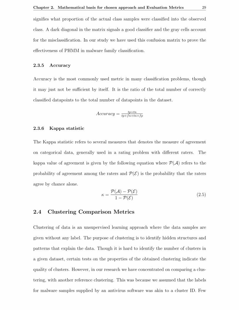
2.3.5 Accuracy
Accuracy is the most commonly used metric in many classification problems, though
it may just not be sufficient by itself. It is the ratio of the total number of correctly
classified datapoints to the total number of datapoints in the dataset.
Accuracy = tp+tntp+fn+tn+fp
2.3.6 Kappa statistic
The Kappa statistic refers to several measures that denotes the measure of agreement
on categorical data, generally used in a rating problem with different raters. The
kappa value of agreement is given by the following equation where P(A) refers to the
probability of agreement among the raters and P(E) is the probability that the raters
agree by chance alone.
κ =P(A)− P(E)
1− P(E)(2.5)
2.4 Clustering Comparison Metrics
Clustering of data is an unsupervised learning approach where the data samples are
given without any label. The purpose of clustering is to identify hidden structures and
patterns that explain the data. Though it is hard to identify the number of clusters in
a given dataset, certain tests on the properties of the obtained clustering indicate the
quality of clusters. However, in our research we have concentrated on comparing a clus-
tering, with another reference clustering. This was because we assumed that the labels
for malware samples supplied by an antivirus software was akin to a cluster ID. Few

Chapter 2. Mathematical basis for chosen approach and Evaluation Metrics 30
clustering methods were applied to the data and then compared to the ground labels(for
clusters). The commonly used metric in cluster comparison were again Precision and
Recall. Let us carefully look at these measures.
2.4.1 Precision and Recall
Let M denote a collection of m malware instances to be clustered. Let C = {Ci}1≤i≤c
and D = {Di}1≤i≤d be two partitions of M , and let f : {1 . . . c} → {1 . . . d} and
g : {1 . . . d} → {1 . . . c} be functions. Many prior techniques evaluated their results
using two measures:
Precision(C,D) = 1m
∑ci=1 |Ci ∩Df(i)|
Recall(C,D) = 1m
∑di=1 |Cg(i) ∩Di|
where C is the set of clusters resulting from the technique being evaluated and D
is the clustering that represents the right answer. More specifically, in the case of
classification, Ci is all test instances classified as class i, and Di is all test instances
that are really of class i. In clustering, there is no specific label to a cluster in D
that corresponds to a cluster in C, as in classification. So usually we resort to have
the functions that map the clusters between C and D as the cluster that has maximal
overlap with the one in its domain. Or
fi = argmax i′ |Ci ∩Di′ |
gi = argmax i′ |Ci′ ∩Di|
The pros and cons of using different metrics are explained in detail, with respect to the
problem in malware clustering. This is done so because the reference clustering that we
use for evaluation, matters in determining the effectiveness of one malware clustering
method over another. F-Score can be calculated using the same formula mentioned in
the classification metrics section.
Chapter 3
Malware Classification and
Clustering using PHMM based
approach
3.1 Initial Experiments
The initial experiments are conducted on the publicly available dataset that comprises of
behavior reports generated by CWSandbox, for nearly 3130 malware binaries collected
over three years from many sources[3]. The malware files in this dataset were annotated
by choosing the majority of the labels given independently by six different anti-virus
products. Each malware family has a number of files ranging from 30 to 300. The details
of the reference dataset that we have used for our experiments is shown in Figure 3.1. It
says the name of the malware and the corresponding number of files belonging to each
family. The distribution of files over these 24 classes is similar to real world situation in
the sense that it is skewed. The initial experiments were conducted for the problem of
malware classification, in which case we assume the label given by antivirus as ground
truth label.
Our approach to the classification problem employing PHMM employs the following
steps:
1. The behavior reports (which are XML files) obtained from the dynamic analysis
31

Chapter 3. Malware Classification and Clustering using PHMM based approach 32
Figure 3.1: The different malware families and the number of files in each, as in Malheur referencedataset[19]
tool such as CWSandbox(currently called the GFISandbox), can be encoded using a
more simpler representation such as the MIST[3]. The MIST format that we chose for
experiments can be processed at different levels considering how much of system call
argument information we look at. Refer to Fig. 3.2 for a sample MIST encoding. We
can also directly encode every unique type of a system call to a particular alphabet in
the range (A-T) and eventually the behavior report looks like a protein sequence.
2. A small number of such sequences belonging to a known malware family (ranging
from 3 to 15 files) is given to a multiple sequence alignment module to get an alignment
file.
3. The multiple alignment file for a malware family is used for constructing a profile
hidden markov model for that family. Many such HMM profiles can be combined to
create a malware profile database.
4. When a new malware file is given, it is again encoded as a sequence and searched for
in the malware profile database. The profile HMM gives a score for the most similar
malware families for that new sequence.The one with the highest score is taken as the

Chapter 3. Malware Classification and Clustering using PHMM based approach 33
malware class prediction.
Given that we see how PHMM is a very effective method for doing sequence based
modeling, we will look at how the method is practically applied for our problem in
dynamic malware analysis involving classification and clustering in the next chapter, in
detail.
3.2 Methodology
The main reason for us to choose this approach for solving the problem of finding mal-
ware similarity is because the behavior of malware program has variablility, yet has
a characteristic signature reflected in the sequence of system calls. For example if we
look at the CWSandbox reports for two malware programs from same family, we notice
that a sequence of malicious actions is preserved, interspersed with some other actions
introduced to confuse the malware detection system.
In this thesis , it is shown that polymorphic malware are better detected when we
look at their behavior, where we expect a certain common sequence of actions to be
preserved, in spite of obfuscation in the code. We choose PHMM mainly because it
intuitively fitted the kind of sequence search problem, which we have in classifying
malware behavior. The initial experiments are done on a fairly diverse dataset that
has close to 24 families of malware and we see that the results are quite promising.
The F-scores for most of the classes considered,(including polymorphic families) are
above 0.96. This way, we show that the method is comparable to some of the best
of the techniques used for this problem. Later we extend the experiments on a larger
and more varied dataset of malware infected files, which poses more challenges to the
analysis and grouping of similar files. The challenges are explained and the results of

Chapter 3. Malware Classification and Clustering using PHMM based approach 34
using PHMM models on the dataset is also presented.
The Profile Hidden Markov Model is a probabilistic approach that developed specially
for modeling sequence similarity occurring in biological sequences such as proteins and
DNA[6][8]. It is also a faster alternative to the traditional deterministic approaches used
in sequence matching [8]. It is a modified implementation of HMM, which is basically
a generative model and constructs a probabilistic finite state machines. For behavior-
based analysis, we again assume that there is a sequence of operations common for a
virus family and for a presented new sequence we would like to find the best known
match from the database.
A hidden markov model (HMM) is very suitable for probabilistic modeling of such
sequences, which is evident from past works. Thus it can be used for modeling different
classes of malware. But as we have discussed above , there might be additions, deletions
or changes to the system calls for different programs within same malware family. The
profile HMM is exactly designed to model this kind of problem, because it also has
non-emitting states or the delete states. The reports are available in the MIST format
too. For our experiments, we consider only the MIST Level 0 in the reports.That is,
we look at only the system call type and not the argument values. This level is actually
sufficient for discrimination of various classes of malware.
The MIST Level 0 reports have close to eighty five different mist codes or system
call operations, out of which, 20 operations are very frequent. The Fig 3.2(a) shows the
XML representation of a dynamic analysis report on CWSandbox. The corresponding
MIST representation is seen in 3.2(b). As the figure explains the corresponding infor-
mation are coded in way such that the most important and relatively static information
about the system call is on the left and less important parameters (those that change
in value for different executions) such as memory addresses or file locations are towards

Chapter 3. Malware Classification and Clustering using PHMM based approach 35
Figure 3.2: Sample of MIST representation of a portion of CWSandbox report[3] (a) and (b)
the right. Now we map every category operation code with a unique alphabet in the
range [A-T]. The remaining category operation codes are also mapped to alphabets in
the accepted range.This facilitates the sequence representation to be compatible with
the protein sequence format such as the FASTA or the STOCKHOLM formats.
Now for every family of malware, say Allaple, we choose few (typically between 5-
20) files and add their sequence representation to FASTA (*.fa) file. The number of
samples was chosen proportional to the number of samples in the dataset and often
chosen at random. And when more than 10 samples were used for a family, we resorted
to choosing samples that had varying sequence length. This variability would help in
building better models that give higher accuracy in prediction. The FASTA file with
the sequences is given to the multiple sequence alignment module and the output is
an aligned FASTA (*.afa), which has the multiple alignment. The alignment file for
that malware family is now given to the hmmbuild step in hmmer, which now creates
a profile HMM for the class.This is done for all the families of malware. The malware
profile database is the concatenation of all the HMM profiles created for the known
malware families in hand.

Chapter 3. Malware Classification and Clustering using PHMM based approach 36
Presented with an unknown malware instance, we convert the MIST encoded file to
a FASTA sequence file. The hmmsearch operation of the hmmer triggers a search on
the profile database. The result of the hmmsearch operation gives the scores for the
different malware families profiles, that were closely related to the presented sequence.
The score values for the overall sequence match and best domain matches are obtained.
Choosing the family which gets the maximum score, gives the classification result. The
score differences between the families can also help us get some insight into how close
the match was, to each of it.
The hmmsearch operation takes longer time for identifying very long sequences
with more than 50000 operations in a single report. Multiple sequence alignment and
hmmsearch operations were run on a system with quad-core Intel(R) Xeon(R)E5440 @
2.83GHz processor with 32GB of RAM. Some sequences in the family SALITY were
too long and we haven’t used them for testing in our experiment. But we plan to look
at how to handle such sequences in our future work.
3.3 Results
We already saw that, around 5 to 20 files are used to construct the profile HMM for
every malware family considered. The testing set consisted of the remaining files in the
dataset[19]. The predictions of the HMM for all the malware programs spanning the
24 families is given in the form of a confusion matrix in Figure 3.4. We see that the
overall accuracy for the dataset is around 95% and the classification accuracy for most
of the classes is close to 100%. This shows that our approach is comparable with the
state-of-the-art approaches as the Malheur [1], in terms of prediction accuracy.
The overall accuracy rate over the entire dataset is about 0.964. The accuracy of

Chapter 3. Malware Classification and Clustering using PHMM based approach 37
classification for every class of malware is shown as a histogram in the Figure 3.3(a). We
see that for most of the classes the accuracy is close to 1.0. For classes such as Allaple,
which is polymorphic, all 300 instances were classified correctly. It was noticed that the
scores given for the dominating profile or malware class was very high when compared
to all other closely matched profiles. Also, whenever there was misclassification, the
difference in the scores for the closely matched profiles is small.
(a) Histogram of classification accuracy (b) Histogram of F-scores
Figure 3.3: (a) Histogram of accuracy and 3.3(b)Histogram of F-Scores
The Figure 3.3 b) shows a plot of the F-scores and Figure 3.3 a) shows that of
the accuracies obtained for the classification results. The average F-score taken over
most of the classes are more than 0.96 and there are families like Looper, Adultbrowser
etc. with values 1.0. We would like to compare this with results from [1] and [12]
which give average F-scores of about 0.88 and 0.97 respectively, which are considered
state-of-the-art.
The confusion matrix for the multi-class prediction of malware families is presented in
the Figure 3.4. By observing this matrix we see how the diagonal blocks are dark,owing
to high prediction accuracy. There are lighter grey blocks outside the diagonal reflect-
ing the proportion of files that were misclassified for every target malware family. The
confusion plot gives us some insight on how closely related different families are.

Chapter 3. Malware Classification and Clustering using PHMM based approach 38
Figure 3.4: Confusion matrix for malware classification
For some classes like Ldpinch, owing to the small size of the reports and high vari-
ability, the accuracy is low. Programs of the family virut and rbot are very close in the
behavior pattern which is reflected in the accuracy.
3.4 Closer look at malware analysis
In this section, we extend our approach on larger collection of malware to show its
usefulness in real-time malware analysis, motivated by the initial results. The publicly
available malheur application dataset[19] has close to about 400 different families of
malware reports available, on which we wanted to test our approach and do a compre-
hensive study.

Chapter 3. Malware Classification and Clustering using PHMM based approach 39
3.5 Challenges in practice
It is known that there are many challenges in the analysis on such large and varied
dataset when using the PHMM approach. To encode a broader range of MIST instruc-
tions, a better and efficient encoding scheme was required. The encoding also had to
take into account the larger range of malware classes that had to be analysed. Since
there are many classes of malware with just very few (1 to 3) instances available for
analysis, a pure classification approach may not be very suited. So we resort to a
clustering approach that would work on the PHMM scores that we obtain for every
malware report against stable malware profiles.
If we assume the malware family name given by an antivirus as the ground truth, then
the cluster size distribution for the labeling is still skewed. So in addition to precision
and recall for clustering, measures like dispersion index are also calculated to assess the
purity of the clusters. The reference dataset that was used in our initial experiments
has a few shortcoming when evaluating the performance of any methodology. The be-
haviour of different classes of malware in the dataset were distinct from one another. As
pointed in a work by Li et al [26] , most of the discriminative classification models built
on such datasets give good results and the effectiveness of one method over another does
not account for the intrinsic characteristics of a malware. In the same work it is been
analysed that biased cluster size distribution in the dataset reduces the significance of
a high precision and recall of the clustering results of the malware as observed in the
dataset used for a fast scalable clustering approach[12]. Also the issue of inconsistency
in the labels used for this evaluation across different anti-virus vendors renders the eval-
uation metric not so effective. It is pointed that even a plagiarism detection software
gave comparable results for the dataset and metrics while still the Locality Sensitive
Hashing based clustering technique considered in [12] is far more scalable. In essence,
our analysis emphasizes on the clustering of malware mainly based on its behaviour

Chapter 3. Malware Classification and Clustering using PHMM based approach 40
that we obtain and study of malware evolution on this large dataset using the PHMM
approach.
3.6 Detailed Experiments
We present the details of experiments in testing the usefulness of PHMM to create
malware family profiles and how one can use the PHMM scores to cluster a large set
of malware instances. The malware analysis using this approach involves the following
steps.
1. We choose to use the MIST[3] approach for representing the instructions of the
CWSandbox report.
2. The MIST 0 level is what we have used for the current experiments. In future, we
will consider using the arguments of the MIST instructions too (higher mist levels).
3. Since the number of unique instructions in the MIST set is more than the number of
legitimate alphabets in the protein encoding(20), we choose to use an efficient encoding
algorithm which will be described in the following subsection.
4. The choice of the malware instances to create the family’s PHMM profile was an
important question that arose. We have addresed the issue, by choosing the most
variable sequences in terms of the sequence length and malware behaviour.
5. As in the previous experiment, the subsequent steps are the MSA of the chosen
sequences and building of the HMM profiles for those families that we have enough
samples of.
6. The new unseen sequences of all the malware instances are scored against the profile
database. The resulting scores for the top scoring families(above an inclusion threshold)
are then normalised across all known families in the database.
7. This normalised vector is then used for clustering the malware into families. We
have used a fast repeated bisection method for clustering the set of malware reports.

Chapter 3. Malware Classification and Clustering using PHMM based approach 41
3.6.1 Encoding the behaviour reports
The behaviour reports of the malware dataset[19] are encoded using the MIST codes
as in the paper[3]. When converting this encoding to that of the protein sequences we
have fewer codes to represent a larger set of MIST instructions. We resorted to use
the huffman encoding algorithm for the same. The idea behind Huffman coding is to
give less frequent characters and groups of characters longer codes. Also, the coding
is constructed in such a way that no two constructed codes are prefixes of each other.
This property about the code is crucial with respect to easily deciphering the code. We
observed that even in the MIST opcode vocabulary for all of the reports, the frequency
distribution of the opcodes is very skewed and obeys the Zipf’s law. Hence Huffman
coding works as an optimal prefix coding for the behavioral sequences and the data loss
is minimum. The lengths of the sequence also don’t grow beyond a factor of 3. The
smallest amino sequence had about 300 symbols and longest was about 4000 and the
average length was around 1600 characters in the sequence after the multiple alignment
step. Also the rare behaviour opcodes, that occur commonly in an aligned sequence or
that are absent in majority of the aligned sequences for a malware family, PHMM gives
higher probabilities to the Hidden state paths and emission for match or insertion, for
the amino coding symbols representing the opcode. This makes rare events in malware
behaviour, to be captured well by the model.
3.6.2 Incremental setting for the detailed experiments
The dataset that we used for the detailed experiments mainly focuses on the analysis
of the malware families that exhibit varied behaviour across samples. The malheur
application set has malware files spanning over 403 families, among which, around 146
families have more than three samples each. To see how an incremental analysis can
be done, we did a profile creation for about 130 families and the malware belonging

Chapter 3. Malware Classification and Clustering using PHMM based approach 42
to these families were scored over the profile database. This covered about 7700 files
whose precision and recall was about 0.67 and 0.46 respectively.
In the incremental step, we add the PHMM profiles for 15 more prominent families
to the database. The total number of files in the dataset is around 18990 and the
reports of all the 400 families of malware are presented for scoring and later clustering
using a fast recursive bisection method. The vectors of PHMM scores for each report
is normalised and the cosine similarity measure was used for clustering. The recursive
bisection algorithm is very fast and the clustering results for nearly 19000 malware
reports was available in less than one minute. This is of a great advantage in malware
analysis where thousands of files are typically getting uploaded everyday for analysis.
The classification results for some of the initially seen samples from newly added families
(in the incremental) can be explained with the help of phylogenetic analysis that will
be introduced in the coming section. It is assumed that, at some point of time the
phylogenetic analysis on the aligned MIST sequences helps us discover a new class
of malware branching steadily from an existing family. Once that discovery is done,
the exemplary samples of the new family is used for building its own profile and the
database is updated. However, completely new families of malware generally do not
surface on the web so frequently as the polymorphic variants or extensions of already
existing families of malware. The results of the final clustering is shown in Table 3.1.
The clusterings obtained on this dataset with n-gram features (with n = 4) (malheur
approach) and the proposed method with PHMM scoring features, are compared. We
obtained a higher precision in our method slightly. The recall going down is not a bad
sign since we have more even-sized clusters than the malheur approach. The number of
clusters was varied and was seen to give steady precision and recall for values around
n = 400, which is close to the true number of labels in the dataset. The comparison of

Chapter 3. Malware Classification and Clustering using PHMM based approach 43
Table 3.1: Malware Clustering Comparision of PHMM based method and N-grams methodFeatures Precision Recall Number of clusters
PHMM Scores 0.7058 0.3106 4004-gram frequencies 0.7000 0.3700 400
the two clusterings was done using the function that mapped the clusters with maximum
intersection of data points, as explained in the subsection 2.4.1 in Chapter 2.
3.7 What is Phylogeny?
The phylogenetic analysis is usually done in the field of evolutionary biology to find
the hierarchical relationships between the organisms belonging to different taxonomic
groups that form the leaves in the tree. The physical or the genetic characeteristics
are used for the same. The cladograms or the phylogenetic trees are constructed with
the branch lengths representing the evolutionary distance between the organisms in
consideration.
The trees can be built from two forms of the genomic data. They are the distance
matrices for the genetic sequences and the molecular data comprising the aligned se-
quences themselves. The distance methods build the phylogenetic tree by clustering the
sequences based on their distances obtained from the matrix, in an iterative manner.
Character-based tree building methods can use both types of data, and search for the
best hierarchical tree from a set of possible tree topologies. They are slower than the
distance methods as they come with optimality guarantees, but there are heuristics
that speed up the process.
3.7.1 Malware Phylogeny
The term malware is in common use as the generic name for malicious code of all
sorts, including viruses, trojans, worms, and spyware. Malware authors use generators,
incorporate libraries, and borrow code from others. Malware also frequently evolves due
to rapid modify-and release cycles, creating numerous strains of a common form. The

Chapter 3. Malware Classification and Clustering using PHMM based approach 44
result of this reuse is a tangled network of derivation relationships between malicious
programs. In biology such a network is called a phylogeny; an important problem
in bioinformatics is automatically generating meaningful phylogeny models based on
information in nucleotide, protein, or gene sequences. Generating malware phylogeny
models using techniques similar to those used in bioinformatics may assist forensic
malware analysts. The models could provide clues for the analyst, particularly in terms
of understanding how new specimens relate to those previously seen. Phylogeny models
could also serve as a principled basis for naming malware. Despite a 1991 agreement on
an overall naming scheme and several papers proposing new schemes, malware naming
continues to be a problem in practice [52][53]. We hope that using phylogenetic trees
built from malware behaviour, naming conventions and the virus removal methods can
be more standardised, than how it is done now.
Phylogeny from Our Observations
The tool ClustalW was used for phylogenetic analysis of the encoded MIST sequences of
the malware. It takes in the prealigned homologous sequences, initially computes rough
distance matrices based on pairwise alignment scores. It then uses a simple Neighbor-
Joining clustering method to cluster the leaves of the tree under branches. In biology,
the homologous sequences refer to the nucleic acid or protein sequences that are similar
because they have a common evolutionary origin. The phylogenetic tree for the families
Virut and Kies are shown in Figure 3.5. The initially seen few samples of Virut were
misclassified as Kies and it is seen that the tree reflects the common behaviour that
they share. A similar tree for the families Palevo and Buzus are shown in Figure 3.6.
In the trees the length of the branch is proportional to the distance of the leaf or leaves
from that node to the parent. Palevo was a worm that surfaced in 2009 and it opens
a back door on the compromised computer and attempts to connect to the following
IRC server to receive commands and the Buzus shared similar behaviour too. In the
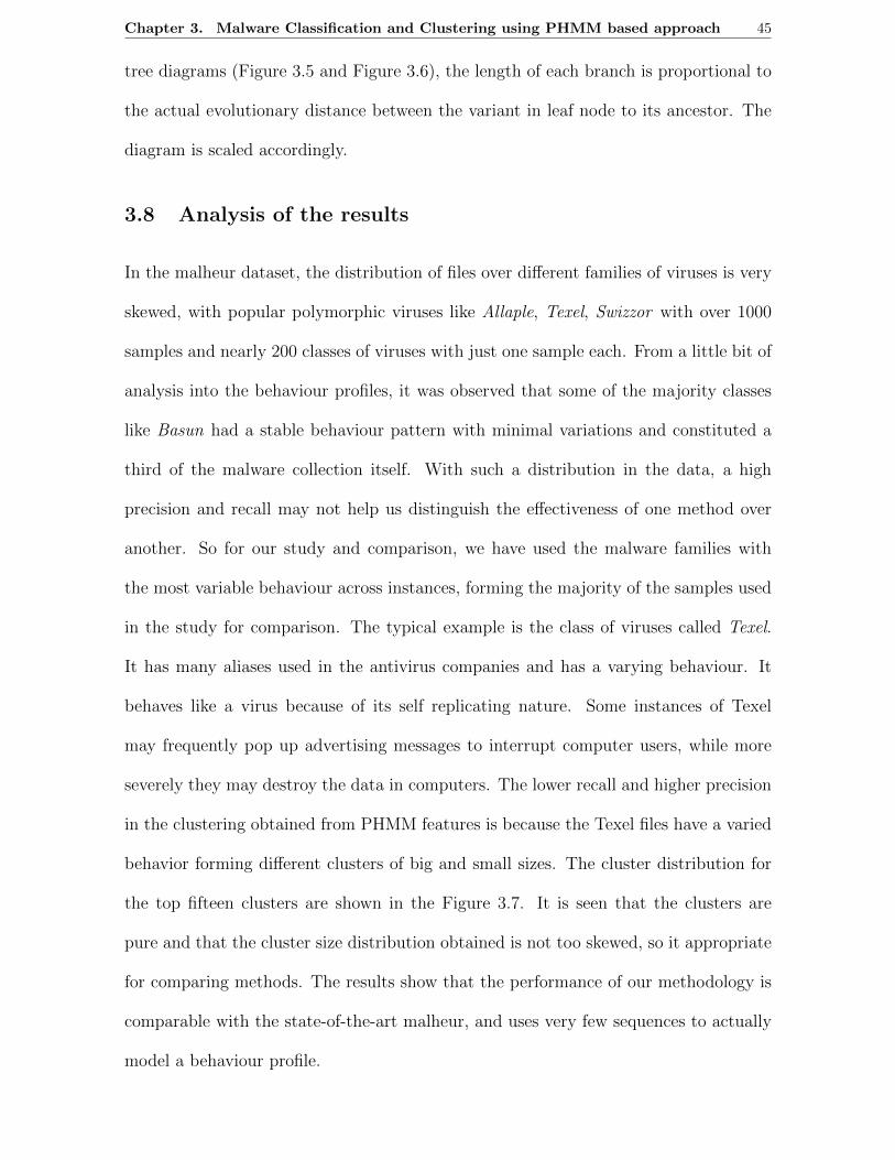
Chapter 3. Malware Classification and Clustering using PHMM based approach 45
tree diagrams (Figure 3.5 and Figure 3.6), the length of each branch is proportional to
the actual evolutionary distance between the variant in leaf node to its ancestor. The
diagram is scaled accordingly.
3.8 Analysis of the results
In the malheur dataset, the distribution of files over different families of viruses is very
skewed, with popular polymorphic viruses like Allaple, Texel, Swizzor with over 1000
samples and nearly 200 classes of viruses with just one sample each. From a little bit of
analysis into the behaviour profiles, it was observed that some of the majority classes
like Basun had a stable behaviour pattern with minimal variations and constituted a
third of the malware collection itself. With such a distribution in the data, a high
precision and recall may not help us distinguish the effectiveness of one method over
another. So for our study and comparison, we have used the malware families with
the most variable behaviour across instances, forming the majority of the samples used
in the study for comparison. The typical example is the class of viruses called Texel.
It has many aliases used in the antivirus companies and has a varying behaviour. It
behaves like a virus because of its self replicating nature. Some instances of Texel
may frequently pop up advertising messages to interrupt computer users, while more
severely they may destroy the data in computers. The lower recall and higher precision
in the clustering obtained from PHMM features is because the Texel files have a varied
behavior forming different clusters of big and small sizes. The cluster distribution for
the top fifteen clusters are shown in the Figure 3.7. It is seen that the clusters are
pure and that the cluster size distribution obtained is not too skewed, so it appropriate
for comparing methods. The results show that the performance of our methodology is
comparable with the state-of-the-art malheur, and uses very few sequences to actually
model a behaviour profile.

Chapter 3. Malware Classification and Clustering using PHMM based approach 46
Figure 3.5: Phylogenetic tree for Virut and Kies
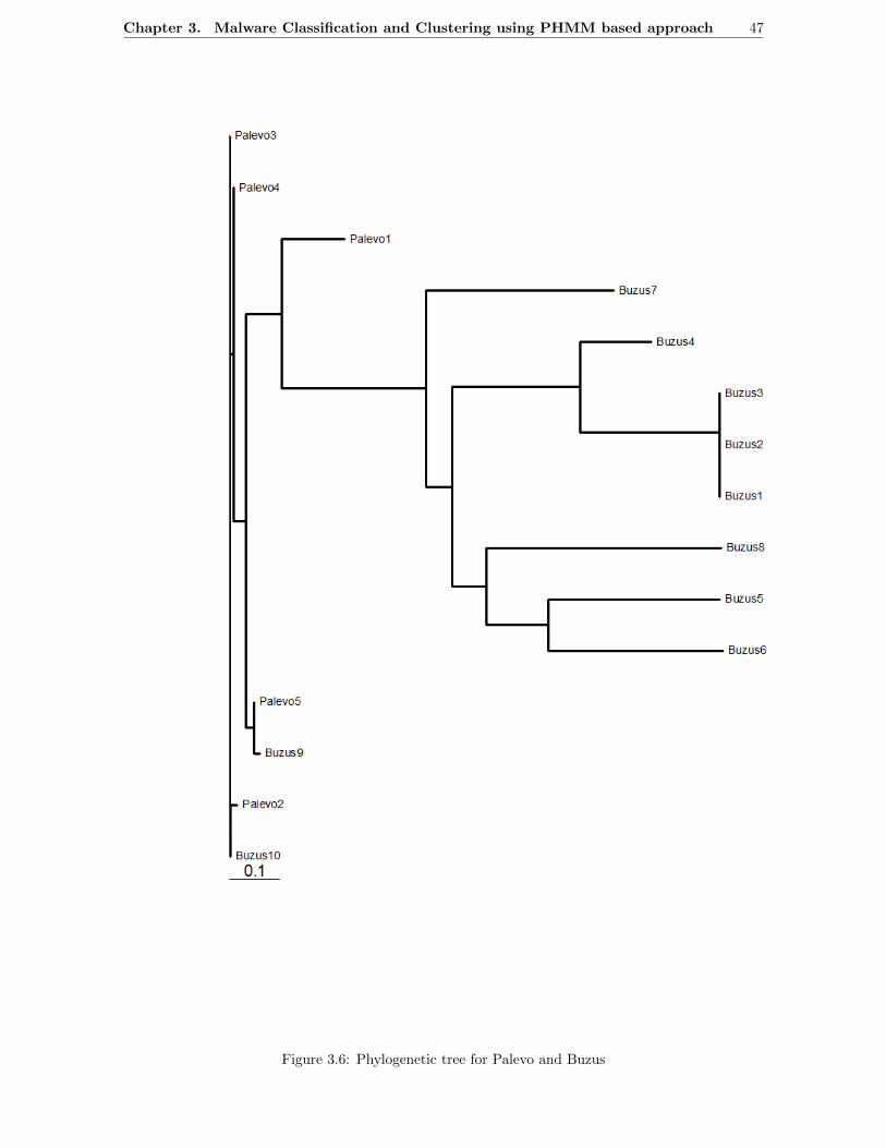
Chapter 3. Malware Classification and Clustering using PHMM based approach 47
Figure 3.6: Phylogenetic tree for Palevo and Buzus
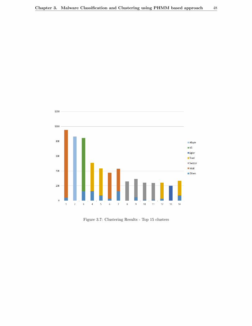
Chapter 3. Malware Classification and Clustering using PHMM based approach 48
Figure 3.7: Clustering Results - Top 15 clusters

Chapter 4
Intrustion Detection in a Data
Stream
Though IDSs can be classified based on a number of attributes, there are two major
classes of IDSs. First of them are misuse-detection systems or the signature-based de-
tection systems that model the patterns of previously known attacks. These could be
hand-crafted signatures or even rules learnt by a system, that characterised a known
attack. These systems are fast in detecting known attacks but are weak in detecting
zero-day attacks. The other class of IDS is the anomaly detection systems, that models
the normal non-malicious behavior of the system and flags any deviation from that as
abnormal. They are very effective in identifying new unseen attacks, but suffer from the
problem of high false-positive rates in detecting attacks. Some of the modern IDS/IPS
solutions use a combination of rules, statistical, and deep packet inspection techniques
for identifying attacks. The signature based detection is effective in identifying and ex-
isting class of attack, but the signature database requires constant update from someone
with expert knowledge.
49

Chapter 4. Intrustion Detection in a Data Stream 50
4.1 Brief Introduction to machine learning
Machine learning deals with the construction and study of systems that can learn from
data. In figure 4.1 , we have shown the broad classes of learning algorithms with ex-
amples. The table also talks briefly the differences in the different learning approaches.
Though there are technically 4 classes of algorithms, the Supervised and Unsupervised
learning algorithms are very prominently used in the problem of intrusion detection.
Machine learning has historically concentrated on learning from small numbers of ex-
amples, because only limited amounts of data were available when the field emerged.
Though not currently in practical use, sophisticated algorithms that can learn highly
accurate models from limited training examples have been explored in the field of ma-
chine learning. It is commonly assumed that the entire set of training data can be
stored in working memory. More recently the need to process larger amounts of data
has motivated the field of data mining.It explores methods to reduce computation time
and memory when working with large, static datasets. If the data cannot fit into mem-
ory, it may be necessary to sample a smaller training set. Otherwise, an algorithm
may process only subsets of data at a time. Commonly the goal is to create a learning
process that is linear in the number of examples. The essential learning procedure is
treated like a scaled up version of classic machine learning, where a set of training
examples are processed to output a final static model. The data mining approach does
not address the problem of a continuous supply of data even if it allows larger data sets
to be handled. Typically, a model that has already been learned cannot be updated
with new information arrives. Instead, the entire training process must be repeated
with the new examples included. This limitation can be inefficient and undesirable for
certain situations.

Chapter 4. Intrustion Detection in a Data Stream 51
4.2 Stream-based learning paradigm
The data stream paradigm is used to address the problem of continuous data. Algo-
rithms written for data streams can naturally cope with data sizes many times greater
than memory, and can extend to challenging real-time applications not previously tack-
led by machine learning or data mining. The core assumption of data stream processing
is that training examples can be briefly inspected a single time only. The algorithm
processing the stream has no control over the order of the examples seen, and must up-
date its model incrementally as each example is inspected. Another useful property, the
”anytime” property, requires that the model be applied at any point between training
examples. Studying purely theoretical advantages of algorithms is certainly useful , but
the demands of data streams require this to be followed up with empirical evidence of
performance. Claiming that an algorithm is suitable for data stream scenarios raises the
doubt as to whether these claims cannot be backed by reasonable empirical evidence.
Data stream classification algorithms require proper evaluation practices. The evalua-
tion should allow users to be sure that particular problems can be handled, to quantify
improvements to algorithms, and to determine which algorithms are most suitable for
their problem.
4.3 Intrusion detection systems employing machine learning -
A survey
Intrusion detection systems have evolved a lot since the Denning’s seminal work on
intrusion detection[27]. Besides network-based detection, these systems have also been
used for host protection in the operating system level, by modeling system call sequences[29].
PAYL[35], which is a payload-based network anomaly detection system, models the byte
frequencies in the packet payloads of various lengths and various services. It is proved
to be fast and the problem of retraining the model is also addressed well.

Chapter 4. Intrustion Detection in a Data Stream 52
Figure 4.1: Broad Classification of machine learning
In general, the anomaly detection problem has been solved using different formulations
for the one-class SVM or density-based outlier detection methods.[55][57] The work
on Support vector Data Description(SVDD)[56] introduces the concept of finding a
spherical boundary around the training data considered to be from one single class, say
normal traffic. The problem is formulated as a constrained minimisation problem with
the objective function being the square of radius of a minimal enclosing hypersphere, for
all given training data. A regularisation term with a cost variable is included to avoid
over-fitting problem. The training data is transformed to a higher dimensional hyper-
space using the transformation φ(xi). The centre of the hypersphere is represented by
w. The constraint is that all datapoints xi must lie within the radius of this sphere ,
when transformed to the hyperspace. The basic formulation that is used for the shown
in Equations 4.1 and 4.2 represent the problem, just explained. Once the solution is
found by solving the dual of this problem, for any incoming packet or datapoint it is
enough to find its distance from the center of hypersphere and verify if it is within the
radius. Else the data is flagged as an anomaly.

Chapter 4. Intrustion Detection in a Data Stream 53
minw,R,ξi
R2 + C∑
i ξi
s.t. ‖φ(xi)− w‖22 ≤ R2 + ξi ∀ i (4.1)
ξi ≥ 0 ∀ i (4.2)
The area of intrusion detection is well studied and the use of data-mining and pat-
tern recognition algorithms for the same have been researched. A variety of learning
algorithms such as the SVMs, decision trees, neural nets etc. have been widely used for
attack detection and classification. In the context of misuse detection, where we try to
model different type of attacks and non-attack data together, a classification approach
is very often used. The main issue in doing research in intrusion detection is the lack
of publicly available dataset that are representative of the current activity patterns.
Most of the previous studies have been done on mainly two publicly available datasets.
They are the DARPA Dataset 1999 and the KDD Cup 99 Intrusion detection dataset.
Though the relevance of these synthetic datasets is much argued about in literature,
they do serve as a benchmark for analysis of various new techniques used in IDS.[37].
Lee and Stolfo [32] proposed the association rules algorithm and the frequent episodes
algorithm for Intrusion Detection. These algorithms were used to compute audit record
patterns, and propose an agent-based architecture for updating the models from the
statistics collected over time. Several learning algorithms like the neural networks,
functional networks, adaptive regression splines have all been used on the features ob-
tained from Lee’s method. The winner of the 1999 KDD cup contest had employed an
ensemble of decision trees with bagged boosting, but different groups published better
methods and algorithms. The work of Mukkamala etal [40] that used the Support Vec-
tor Machines for 2-class classification of attack and non attack records on KDD dataset

Chapter 4. Intrustion Detection in a Data Stream 54
reported a high accuracy of about 99.5%. In order to reduce the size of the dataset,
several researches proposed to apply feature selection methods to the training dataset
( [Chebrolu et al., 2005], [Kayacik et al., 2005] and [Mukkamala and Sung, 2002]).
4.4 Commonly used datasets for validation of an IDS
4.4.1 DARPA 1999 Dataset for Intrusion Detection
At Lincoln Labs, MIT Lippman etal.,[31]developed an intrusion detection evaluation
test bed which generated normal traffic similar to that on a government site containing
100s of users on 1000s of hosts. More than 300 instances of 38 different automated
attacks were launched against victim UNIX hosts in seven weeks of training data and
two weeks of test data. The attacks were broadly of 4 types namely, probe, denial of-
service (DoS), remote-to-local (R2L), and user to root (U2R) attacks. They analysed
the performance of 6 different IDSs that had handcrafted rules or signatures, or expert
systems to detect the attacks.Their results suggested that further research had to focus
on developing techniques to find new attacks instead of extending existing rule-based
approaches. This dataset that was created for the test-bed is most commonly known
as the DARPA 1999 dataset[30] for Intrusion Detection.
Lee and Stolfo [32] proposed two general data mining algorithms that were the
association rules algorithm and the frequent episodes algorithm for Intrusion Detection.
These algorithms were used to compute the intra- and inter-audit record patterns,
on the system call traces and network audit logs and they propose an agent-based
architecture for updating the models from the statistics collected over time. In their
subsequent work[33], a detailed data mining framework was proposed. The features
that are collected from network dump files and system audit logs were clearly classified

Chapter 4. Intrustion Detection in a Data Stream 55
as connection-based and time-based features. The framework made it easy for crafting
rules for detection of different types of attacks based on the ’features’ that they built.
PAYL[35], which is a payload-based network anomaly detection system, models the
byte frequencies in the packet payloads of various lengths and various services. It is
proved to be fast and the problem of retraining the model is also addressed well.
The KDD Cup 99 contest winner employed an ensemble of decision trees with bagged
boosting. Several authors in the literature have used this dataset in order to test their
classifiers and trying to improve the results achieved by the winner. Earlier studies have
utilized neural networks and support vector machines (SVMs) [40]. These approaches
were used again later by Fugate and Gattiker (2003) together with an ANOVA model,
and they outperformed some of the results of the KDD winner, but the drawback
of these methods is that they are very time and computational consuming and it is
necessary to deal with reduced training datasets. Lately, functional networks were also
applied to this dataset, obtaining similar results and the same inconvenient. In order
to reduce the size of the dataset, several researches proposed to apply feature selection
methods to the training dataset [40] [41]. However, these works were more focused in
determining the more relevant features than in achieving better performance with fewer
attributes.
4.4.2 The KDD Cup 1999 Dataset
The KDD Cup 99 dataset, taken from the DARPA IDS evaluation dataset [31], was
used for the KDD Cup 99 Competition[34]. The complete dataset has almost 5 million
input patterns and each record represents a TCP/IP connection that is composed of 41
features that are both qualitative and quantitative in nature[37] [33]. The dataset used
in our study is a smaller subset (10% of the original training set), that contains 494,021
instances and it was already employed as the training set in the competition. For the

Chapter 4. Intrustion Detection in a Data Stream 56
test set, we used the original KDD Cup 99 dataset containing 331,029 patterns. Around
20% of the two datasets are normal patterns (no attacks). As for attack patterns, the
39 types of attacks are grouped into four categories[43].
1. Denial of Service (DoS) attacks, where an attacker makes some computing or
memory resource too busy or too full to handle legitimate requests.
2. Probe attacks, where an attacker scans a network to gather information or find
known vulnerabilities.
3. Remote-to-Local (R2L) attacks, where an attacker sends packets to a machine over
a network, then exploits machines vulnerability to illegally gain local access as a user.
4. User-to-Root (U2R) attacks, where an attacker starts out with access to a normal
user account on the system and is able to exploit vulnerability to gain root access to
the system.
The 1998 DARPA Intrusion Detection Evaluation Program was prepared and man-
aged by MIT Lincoln Labs. The objective was to survey and evaluate research in
intrusion detection. A standard set of data to be audited, which includes a wide variety
of intrusions simulated in a military network environment, was provided. Lincoln Labs
acquired nine weeks of raw TCP dump data for a typical U.S. Air Force Local Area
Network (LAN). They operated the LAN as if it were a true Air Force environment,
but peppered it with multiple attacks. The raw training data was about four gigabytes
of compressed binary TCP dump data from seven weeks of network traffic, which was
processed into about five million connection records. The two weeks of test data yielded
two million connection records.
Attacks fall into four main categories as explained above in KDD 99 Dataset section.
It is important to note that the test data and training data do not have the same
probability distribution (including specific attack types not in the training data). This

Chapter 4. Intrustion Detection in a Data Stream 57
makes the task more realistic. Some intrusion experts believe that most novel attacks
are variants of known attacks and the ”signature” of the latter can be used to catch the
former. The datasets contain a total of 24 training attack types, with an additional 14
types in the test data only.
4.5 Stream based learning algorithm
The incremental learning algorithms are used in KDD systems that operate indefinitely
and continuously arriving examples. There exist a number of online or sequential learn-
ing algorithms that are efficient but offer no performance guarantees.
The Hoeffding Tree algorithm[46] is an anytime algorithm that is used for classification
tasks, and can be used for learning from large datasets. Every example is seen exactly
once. Its performance increases smoothly with time. The Hoeffding Tree algorithm
uses the Hoeffding bound result from statistics to determine the number of examples
necessary to do the testing of an attribute value.
The MOA framework [45] implements several algorithms that learn from data streams
in an online fashion. The framework has implementations of the classical Naive Bayes,
Hoeffding trees, Random Hoeffding trees, OZBoost, Weighted Majoriy Algorithm etc.
The OZBoost is a boosting algorithm that uses a forest of hoeffding trees in learn-
ing.The framework also supports the generation of data points as in a stream, with
preset time intervals for a concept drift. Parameters of the learning algorithm such as
the prior distributions and their parameters, number of trees to use for bootstrapping
etc., can also be tuned up.

Chapter 4. Intrustion Detection in a Data Stream 58
4.6 Hoeffding Trees
We shall now look at the Hoeffding tree algorithm in detail. The classification problem
is generally defined as follows. A set of N training examples of the form (x; y) is given,
where x is a vector of d attributes, and y is a discrete class label each of which may
be symbolic or numeric.From this sample data we wish to learn a model y = f(x) that
will predict the classes y of future examples x. One of the most widely-used classifica-
tion methods is decision tree learning. Learners of this type induce models in the form
of decision trees, where each node contains a test on an attribute, each branch from
a node corresponds to a possible outcome of the test, and each leaf contains a class
prediction. The label y = DT(x) for an example x is obtained by passing the example
down from the root to a leaf, and following the branch corresponding to the attribute’s
value in the example. A decision tree is learned by recursively replacing leaves by test
nodes, starting at the root. The attribute to test at a node is chosen by choosing the
best one according to some heuristic measure. Classic decision tree learners like ID3,
C4.5 and CART assume that all training examples can be stored simultaneously, and
are therefore severely limited in the number of examples they can learn from. Disk-
based decision tree learners like SLIQ and SPRINT assume the examples are stored on
disk, and learn by repeatedly reading them in sequentially. While this greatly increases
the size of usable training sets, it can become too expensive. Our goal is to design
a decision tree learner for extremely large datasets. This learner should require each
example to be read at most once, with small processing time. This will make it possible
- without ever storing the examples - to directly mine online data sources, and to build
potentially very complex trees with acceptable computational cost. We achieve this by
noting with Catlett [2] and others that, in order to find the best attribute to test at a
given node, it may be sufficient to consider only a small subset of the training examples
that pass through that node. Thus, given a stream of examples, the first ones will be

Chapter 4. Intrustion Detection in a Data Stream 59
used to choose the root test. We solve the problem of deciding how many examples are
necessary at each node by using the Hoeffding bound (or additive Chernoff bound) [7,
9]. Consider a real-valued random variable r whose range is R. Suppose we have made
n independent observations of this variable, and computed their mean r.
The Hoeffding bound states that, with probability 1−δ, the true mean of the variable
is at least r − ε where
ε =
√R2ln(1/δ)
2n(4.3)
4.6.1 Special properties of the Hoeffding trees
The Hoeffding bound has the very attractive property that it is independent of the
probability distribution generating the observations. The price of this generality is that
the bound is more conservative than distribution-dependent ones (i.e., it will take more
observations to reach the same δ and ε). Let G(Xi) be the heuristic measure used to
choose test attributes (e.g., the measure could be information gain as in C4.5, or the
Gini index as in CART). We wish to ensure that, with high probability, the attribute
chosen using n examples (where n is as small as possible) is the same that would be cho-
sen using infinite examples. Assume G is to be maximized, and let Xa be the attribute
with highest observed G after seeing n examples, and Xb be the second-best attribute.
Let ∆G = G(Xa) − G(Xb) ≥ 0 be the difference between their observed heuristic
values. Then, given a desired δ, the Hoeffding bound guarantees that Xa is the cor-
rect choice with probability 1−δ if n examples have been seen at this node and ∆G > 0.
If d is the number of attributes, v is the maximum number of values per attribute,
and c is the number of classes, the Hoeffding tree algorithm requires O(dvc) memory
to store the necessary counts at each leaf. If l is the number of leaves in the tree, the

Chapter 4. Intrustion Detection in a Data Stream 60
total memory required is O(ldvc). This is independent of the number of examples seen,
if the size of the tree depends only on the true concept and is independent of the size
of the training set.
A key property of the Hoeffding tree algorithm is that it is possible to guarantee
under realistic assumptions that the trees it produces are asymptotically arbitrarily
close to the ones produced by a batch learner (i.e., a learner that uses all the examples
to choose a test at each node). In other words, the incremental nature of the Hoeffding
tree algorithm does not significantly affect the quality of the trees it produces.
4.7 Online learning
Online machine learning is a model of induction that learns one instance at a time. The
goal in on-line learning is to predict labels for instances. For example, the instances
could describe the current conditions of the stock market, and an online algorithm pre-
dicts tomorrow’s value of a particular stock. The key defining characteristic of on-line
learning is that soon after the prediction is made, the true label of the instance is dis-
covered. This information can then be used to refine the prediction hypothesis used by
the algorithm. The goal of the algorithm is to make predictions that are close to the
true labels.
More formally, an online algorithm proceeds in a sequence of trials. Each trial can
be decomposed into three steps. First the algorithm receives an instance. Second
the algorithm predicts the label of the instance. Third the algorithm receives the
true label of the instance. The third stage is the most crucial as the algorithm can
use this label feedback to update its hypothesis for future trials. The goal of the
algorithm is to minimize some performance criteria. For example, with stock market

Chapter 4. Intrustion Detection in a Data Stream 61
prediction the algorithm may attempt to minimize sum of the square distances between
the predicted and true value of a stock. Another popular performance criterion is to
minimize the number of mistakes when dealing with classification problems. In a two-
class classification scenario, the N training set instances (x, y) are given. The incurred
loss for a wrong prediction yt is given by the loss function `(yt, yt), at the third stage.
4.7.1 Online Prediction from Experts
A general online prediction problem proceeds as follows.
Online (binary) prediction using multiple experts
For t = 1, . . . , T :
– Receive instance xt ∈ X
– Receive expert predictors ξ1(xt), . . . , ξN(xt) ∈ {±1}
– Predict yt ∈ {±1}
– Receive true label yt ∈ {±1}
– Incur loss `(yt, yt) If yt 6= yt
– Modify predictor function for yt
4.7.2 Weighted Majority algorithm
Weighted Majority Algorithm (WMA) is a meta-learning algorithm used to construct a
compound algorithm from a pool of prediction algorithms, which could be any type of
learning algorithms, classifiers, or even real human experts. The algorithm assumes that
we have no prior knowledge about the accuracy of the algorithms in the pool, but there
are sufficient reasons to believe that one or more will perform well. The algorithm uses
a multiplicative update on the weights, for the predictors whose predictions go wrong
in every round by a factor η > 0 Consider a two-class classification scenario where the
N training set instances (x, y) are given. The weights w are initialised equal for all
the predictors (or hypothesis or classifiers) in consideration. When the first instance

Chapter 4. Intrustion Detection in a Data Stream 62
is presented the algorithm goes by the decision of the majority of the classifiers. Now
the weights are reduced by a multiplicative factor η > 0, for those classifiers that erred.
And the process iteratively continues for all the training instances in the sequence.
Weighted Majority Algorithm
Initiate weights w1i = 1∀i ∈ [N ]
Choose parameter η > 0 that would be used in the weight update rule.
For t = 1, . . . , T :
– Receive instance xt ∈ X
– Receive expert predictors ξ1(xt), . . . , ξN(xt) ∈ {±1}
– Predict yt = sign(∑n
j=1wtj.ξ
tj) (majority vote)
– Receive true label yt ∈ {±1}
– Incur loss `(yt, yt)
– Update:- If yt 6= yt
∀i ∈ 1 . . . N
wt+1i ← wt
i exp(η.I(yt 6=ξti ))
There are good performance guarantees for the weighted majority algorithm.
4.8 Experiments and Results
We have for the first time used and compared the stream learning algorithms to perform
the multilabel classification of attack and normal data on the KDD Cup1999 dataset.
Several algorithms like the Naive Bayes, Hoeffding Trees, Weighted Majority algorithm,
RandomHoeffding trees etc. were used and the classification performance on the whole
of dataset were studied. The classification accuracies of various algorithms were com-
pared. We notice that the Hoeffding trees and Random Hoeffding trees perform better
in terms of evaluation time and accuracy as the data size grows, whereas Naive Bayes
performs poorly as the data size grows.

Chapter 4. Intrustion Detection in a Data Stream 63
Table 4.1: Accuracies and Kappa-statistic for various Stream learning algorithms on the KDD Cup 99dataset
Algorithm Accuracy Kappa Model ParametersHoeffding Trees 99.4069 98.9841 Gaussian10
Random Hoeffding tree 98.7202 97.8121Weighted Majority 99.9266 99.8743 HT,HT-NB,HT-NBAdaptive,NB
NaiveBayes 95.6028 92.5854
The weighted majority algorithm[48] is an online method that gives a weighted deci-
sion from the predictions of four different classifiers, which explains the increase in its
evaluation time, inspite of the high accuracy. It is noted that, with the first 1 million
examples, Hoeffding Tree predictor gets the maximun weight of about 0.98, when other
classifiers get rest of the weight, over 1. The weights vary very little from there and
ends at 0.994 for HT,0.03 each for Random HT and Naive Bayes. The online algo-
rithms also generally don’t have the i.i.d assumptions on the training and testing data.
It allows us to see, how every component algorithm predicted over a length of time,
which is reflected in its weight. Thus, Hoeffding trees are proven to perform the best
of all in terms of performance and speed. This shows the need for looking closely into
incremental learning for IDS, as there will be space and time constraints when learning
from huge data.
The incremental learners perform well with time, even when there is a concept drift
in the data. Most previous results on KDD Cup 99 dataset[40][43][44], were done on
the 10% Train and Test sample dataset whereas we use the complete dataset with over
4.8 milion samples and the dataset we used has 22 classes of attacks and 1 class of
normal patterns.
The results for different algorithms are tabulated in Table 4.1. The Naive bayes method
was used as a baseline for batch processing method. And the results for Hoeffding trees
with Gaussian priors (with SD = 10.0) were shown to have an accuracy of 99.409.
Random Hoeffding trees (where a subset of features are only used at each step) give a
better accuracy. The online weighted majority algorithm that combined the decisions

Chapter 4. Intrustion Detection in a Data Stream 64
from other classifiers like Hoeffding Trees, Hoeffding Trees with Naive bayes assumption
and Plain Naive Bayes algorithm was seen to work the best. The Figures 4.2 and 4.3
show the graphical comparison of the accuracies and kappa values with every sample,
for the algorithms in study. It is clearly seen that performance of Naive Bayes drops
with time when the number of samples keep increasing. Whereas the other stream
algorithms perform steadily better with more samples. In terms of CPU execution
times, Hoeffding and Random Hoeffding trees learn the model under 100 ms for the
same data. The comparison of CPU execution times of these algorithms with growing
sample sizes is shown in Figure 4.4. The above results encourages us to look more deeply
at the learning setting in the Intrusion Detection problem. If we can obtain a tagged
dataset at any point, the stream learning algorithm can incrementally update the model
for the newly accounted attacks and benign traffic and not lose prior knowledge too.
The online learning algorithms are analysed and compared against each other based on
the factor of Regret as opposed to the Empirical risk as in a batch learning setting. Fast
optimisation algorithms such as the stochastic gradient methods can be used in case of
high dimensional data as in the case of IDS problem. When the power of hardware is
utilised with these powerful algorithms, we can surely see some improvements in the
performances of statistics based IDSs.

Chapter 4. Intrustion Detection in a Data Stream 65
Figure 4.2: Accuracy Comparison Graph
Figure 4.3: Kappa Comparison Graph)

Chapter 4. Intrustion Detection in a Data Stream 66
Figure 4.4: Evaluation Time (in CPU secs)

Chapter 5
Conclusion
In this chapter we will review the main contributions of this thesis and directions for
future work.
5.1 Contribution of the thesis
From earlier research work, we see that polymorphic malware are better detected when
we look at their behavior, where we expect a certain common sequence of actions to
be preserved, in spite of obfuscation in the code. In this thesis, we have shown that
Profile Hidden Markov Models are very effective mainly because it intuitively fitted in
solving the kind of sequence search problem, which is also very commonly encountered
in bio-informatics. It has been experimentally verified that, even with limited examples,
accurate models can be built and the results using these models were comparable to
some of the best of the techniques used for this problem. The initial set of experiments
were done on a diverse set of 24 malware families and the PHMM models were used for
classification.
Later we extended the experiments on a larger and more varied dataset of malware
infected files, which poses more challenges to the analysis and grouping of similar files.
The challenges are explained and the results of using PHMM models on the dataset
is also presented. Malware clustering was performed on the large dataset to cluster or
67

Chapter 5. Conclusion 68
group the files purely based on their behaviour. We also present a phylogenetic analysis
done on the malware samples, purely based on behavioural features. All the results are
comparable to that of state of the art, but this has been acheived with very few training
samples (in between 3-20).
We also proceeded to address the issue of relearning in IDS. A set of stream based
learning algorithms based on the Hoeffding trees have been tried on the KDD Cup 99
Intrusion Detection dataset for the classification of non- attack data and 22 different
kinds of attack. Online learning algorithm such as weighted majority algorithm is
observed to be effective as an ensemble technique in trying to combine many classifiers.
The thesis does a comparison of these algorithms in terms of accuracy, speed and
resource consumption, for the problem of attack classification.
5.2 Directions for future work
The experiments and general trend in security engineering show that, the identifica-
tion and mitigation of malware attack on our networks and systems are going to get
more challenging in the times to come. The polymorphic variants of malware generated
using different virus toolkits pose a major threat and many of the security product com-
panies are moving towards using more elaborate dynamic analysis based or program
verification based techniques for identification and removal of malware. Software vul-
nerabilities in the system and application software also need to be addressed and fixed
with due diligence, when we address the issue of malware. When there are scalable
systems to analyse malware and a standard taxonomy for naming malware families,
it would be easier to compare and evaluate the performance of different anti-malware
products. Though there have been multiple ways suggested through researches, none
of them have been employed across all major anti-virus vendors.

Chapter 5. Conclusion 69
We see from research that dynamic malware analysis is gaining prominence. In a
more recent work,[63], Ying etal., describe a method for extracting a set of minimal ab-
stract behavioral features from the API call sequences, that would serve well for many
graph based data mining approaches. The features they have extracted has advantages
such as resistance to redundant data and ease to embed in very high dimensional space.
With such features made available, more sophisticated machine learning can be done
for classification, detection or clustering of malware.
The advances in the areas of machine learning and statistical analysis can be used
for addressing some of the problems of pattern recognition in computer security. The
recent surge in the consumption and use of mobile devices opens a whole new area in
security research. With the data speeds increasing rapidly in networks, having intelli-
gent IDS that constantly relearns in a dynamic environment, has become all the more
necessary. To support the improvements in software and network speeds, hardware also
have improved a lot, over the years.
The GPUs are the graphics processing units that are separate computational units spe-
cially designed to do hardware optimisation for graphics. These units are much faster
than CPUs since they have the capacity of running several parallel threads. Having
GPUs takes away significant computing load from the CPU for graphic-rich applica-
tions and systems. Slowly GPUs have been utilised for other non-graphic computational
purposes and the advent of architectures such as CUDA (compute unified device archi-
tecture) and standards such as OpenCL have made a breakthrough in fast and parallel
computing. It is evident from previous research the GPU tends to improve the perfor-
mance of CPU-intensive operations, so it is possible to load some of the computations
in the anti-virus program to the GPU. Typically this could be done for fast signature

Chapter 5. Conclusion 70
matching techniques used in popular anti-virus. In fact, the anti-virus makers Kasper-
sky released a GPU version which they have said runs 360 times faster than a CPU
version[68].
We also see some recent work on utilising GPUs for multiple pattern matching algorithms[66].
This paper describes how the GPUs were used for comparing the contents of single
packet in parallel, during the phase of deep packet inspection. In experiments, it is
seen that the proposed algorithm gives twice the performance of the existing multi-
pattern matching algorithm (WM algorithm) that was already used in the Snort IDS.
As always, in the area of security, there is also the flip side to the story involving GPUs.
A recent work describes a prototype that was developed to show how polymorphic mal-
ware can evade detection using GPU architecture.
The paper explains that unpacking of the malicious code can be done by GPU and
be placed in memory that is accessible to the CPU. This process calls for the majority
of the code to be written for the GPU, and little that is executed on the Intel x86 archi-
tecture. Thus there are very little remnants of the executed code in the memory. This
could subsequently make it harder for the current malware detection solutions that may
use methods such as call graph traces or tainting[65]. GPU assisted malware are even
hard when using reverse engineering techniques because the encoding and decoding of
the virus code is done very quickly on the GPU leaving very little time for analysis.
Even with existing debugging techniques, reverse engineering such code is a challenge
for malware analysts.

References
[1] K. Rieck, P. Trinius, C. Willems, and T. Holz: Automatic Analysis of Malware
Behavior using Machine Learning, In Journal of Computer Security 2011.
[2] K. Rieck, T. Holz, C. Willems, P. Dussel, and P. Laskov, Learning and classification
of malware behavior, in Proc. of DIMVA 2008, pp. 108125.
[3] P. Trinius, C.Willems, T. Holz, and K. Rieck. A malware instruction set for
behavior-based analysis. Technical Report TR-2009-07, University of Mannheim,
2009.
[4] NJ. Yadwadkar,C. Bhattacharya,K. Gopinath,T. Niranjan and S. Susarla, Discov-
ery of Application Workloads from Network File Traces, In Proceedings of the 8th
USENIX conference on File and storage technologies, FAST’10.
[5] C. Willems, T. Holz, and F. Freiling. CWSandbox: Towards Automated Dynamic
Binary Analysis. IEEE Security and Privacy, 5(2), March 2007.
[6] S. R. Eddy. Profile hidden Markov models. Bioinformatics,14(9):755763, 1998
[7] S. R. Eddy. HMMER: Sequence analysis using profile hidden Markov models.
[8] R. Durbin, S. Eddy, A. Krogh, and G. Mitchison. Biological Sequence Analysis:
Probabilistic models of proteins and nucleic acids. Cambridge University Press,
1998.
[9] HMMER Implementation: http://hmmer.janelia.org/
71
REFERENCES 72
[10] Edgar,R.C. (2004) MUSCLE: multiple sequence alignment with high accuracy and
high throughput. Nucleic Acids Res., 32, 17921797.
[11] Bayer, U., Kirda, E., Kruegel, C.: Improving the efficiency of dynamic malware
analysis. In: Proceedings of the 2010 ACM Symposium on Applied Computing,
ser. SAC 10, pp. 18711878. ACM, New York (2010).
[12] U. Bayer, P. Milani Comparetti, C. Hlauschek, C. Kruegel, and E. Kirda. Scalable,
Behavior-Based Malware Clustering. In Symposium on Network and Distributed
System Security (NDSS), 2009.
[13] R. Durbin, S. Eddy, A. Krogh, and G. Mitchison. Biological Sequence Analysis:
Probabilistic models of proteins and nucleic acids. Cambridge University Press,
1998.
[14] A. Moser, C. Kruegel, and E. Kirda. Limits of Static Analysis for Malware Detec-
tion. In ACSAC, pages 421 — 430. IEEE Computer Society, 2007
[15] M. Bailey, J. Oberheide, J. Andersen, Z. M. Mao, F. Jahanian, and J. Nazario, Au-
tomated classification and analysis of internet malware”, In Proceedings of RAID
2007.
[16] T. Lee and J. J. Mody, Behavioral classification in Proc. of EICAR, 2006.
[17] G. Wagener, R.State, A. Dulaunoy: Malware behavior analysis, Journal of Com-
puter Virology(2008) 4:279-287
[18] S. Attaluri, S. McGhee and M. Stump: Profile hidden Markov models and meta-
morphic virus detection, In Journal of Computer Virology(2009) 5:151-169
[19] Malheur Dataset: http://pi1.informatik.uni-mannheim.de/malheur/#dldata
[20] Rabiner, L. R. (1989). A tutorial on hidden Markov models and selected applica-
tions in speech recognition. Proc. IEEE, 77 (2), 257-286.

REFERENCES 73
[21] International Secure Systems Lab, Anubis: Analyzing unknown binaries,
http://anubis.iseclab.org/
[22] S. B. Needleman and C. D. Wunsch. A general method applicable to the search
for similarities in the amino acid sequences of two proteins. Journal of Molecular
Biology, 48:443453, 1970.
[23] M. Apel, C. Bockermann, and M. Meier. Measuring similarity of malware behavior.
In Proc. of 34th LCN 2009. IEEE Computer Society, 2009.
[24] Wang, Y.: Statistical Techniques for Network Security: Modern Statistically-Based
Intrusion Detection and Protection. Inf Sci Ref, Hershey, New York (2009)
[25] J. Kolter and M. Maloof. Learning to detect and classify malicious executables in
the wild. Journal of Machine Learning Research, 2006.
[26] P. Li, L. Lu, D. Gao, and M. Reiter. On challenges in evaluating malware clustering.
In Proceedings of the International Symposium on Recent Advances in Intrusion
Detection, 2010.
[27] D. E. Denning, An Intrusion Detection Model, IEEE Transactions on Software
Engineering, SE-13, pp. 222- 232, 1987.
[28] S. Forrest, S.A. Hofmeyr, A. Somayaji, T.A. Longstaff, A sense of self for unix
processes, in: Proceedings of the IEEE Symposium on Research in Security and
Privacy, Oakland, CA, USA, 1996, pp. 120128.
[29] S. A. Hofmeyr, S. Forrest, and A. Somayaji, Intrusion Detection Using Sequences
of System Calls, Journal of Computer Security, vol. 6, pp. 151-180, 1998.
[30] DARPA Intrusion Detectoin. (1998) Lincoln Laboratory:
www.ll.mit.edu/mission/communications/ist/corpora/ideval/data/1998dat a.html

REFERENCES 74
[31] R.P. Lippmann, D.J. Fried, I. Graf, J.W. Haines, K.R. Kendall, D. McClung, D.
Weber, S.E. Webster, D. Wyschogrod, R.K. Cunningham et al., Evaluating Intru-
sion Detection Systems: the 1998 DARPA Off-line Intrusion Detection Evaluation.
Proc. DARPA Information Survivability Conference and Exposition, 2000, vol. 2.
[32] Lee W, Stolfo S. Data mining approaches for intrusion detection. Proceedings of
the seventh USENIX security symposium, San Antonio, Texas; January 26e29,
1998.
[33] Lee W, Stolfo S, Mok K. A data mining framework for building intrusion detection
models. Proceedings of the IEEE symposium on security and privacy; 1999a.
[34] KDD Cup 1999. Available on: http://kdd.ics.uci.edu/databases/kddcup 99/kdd-
cup99.html, October 2007.
[35] K. Wang and S. Stolfo. Anomalous payload-based network intrusion detection. In
Recent Advances in Intrusion Detection, RAID 2004, pages 203222, September
2004.
[36] D. Dasgupta, Immunity-based intrusion detection system: a general framework,
Proceedings of 22nd National Information Systems Security Conference (NISSC)
(1999) p. 14760
[37] M. V. Mahoney, P. K. Chan, An analysis of the 1999 DARPA /Lincoln Laboratory
evaluation data for network anomaly detection, Technical Report CS-2003-02.
[38] Axelsson, Stefan. Intrusion detection systems: A survey and taxonomy. Vol. 99.
Technical report, 2000.
[39] V. Chandola, A. Banerjee, and V. Kumar, Anomaly Detection: A Survey, Univer-
sity of Minnesota, Tech. Rep., 2007.
[40] S. Mukkamala, G. Janoski, A.H. Sung, Intrusion detection using neural networks

REFERENCES 75
and support vector machines, Proceedings of IEEE International Joint Conference
on Neural Networks (2002) p. 170207
[41] Mukkamala Srinivas, Sung Andrew H, Abraham Ajith, Ramos Vitorino. Intru-
sion detection systems using adaptive regression splines. In: Seruca I, Filipe J,
Hammoudi S, Cordeiro J, editors. Sixth international conference on enterprise in-
formation systems. ICEIS04, Portugal, vol. 3. 2004b. p. 26e33. ISBN 972-8865-00-7.
[42] G. Helmer, J. Wong, V. Honavar, L. Miller, Lightweight agents for intrusion de-
tection,Journal of System Software(2003), pp. 109122
[43] S. Mukkamala, A.H. Sung and A. Abraham, Intrusion Detection Using an Ensemble
ofIntelligent Paradigms Journal of Network and Computer Applications, vol. 28,
no. 2, pp. 167-182, Elseiver, 2005
[44] Naoki Abe , Bianca Zadrozny , John Langford, Outlier detection by active learning,
Proceedings of the 12th ACM SIGKDD international conference on Knowledge
discovery and data mining, August 20-23, 2006.
[45] Albert Bifet , Geoff Holmes , Richard Kirkby , Bernhard Pfahringer, MOA: Mas-
sive Online Analysis, The Journal of Machine Learning Research, 11, p.1601-1604,
3/1/2010
[46] Pedro Domingos , Geoff Hulten, Mining high-speed data streams, Proceedings of
the sixth ACM SIGKDD international conference on Knowledge discovery and data
mining, p.71-80, August 20-23, 2000, Boston, Massachusetts, United States.
[47] Kemmerer, Dick, and Giovanni Vigna. ”Intrusion detection: a brief history and
overview.” Computer-IEEE Computer Magazine 1 (2002): 27-30.
[48] Nick Littlestone and Manfred K. Warmuth. The weighted majority algorithm. In-
formation and Computation, 108:212261, 1994.

REFERENCES 76
[49] Y. Freund, R.E. Schapire. A decision-theoretic generalization of on-line learning
and an application to boosting, J. Comput. System Sci., 55 (1) (1997), pp. 119139
[50] Karim, Md.E., Walenstein, A., Lakhotia, A., Parida, L.: Malware phylogeny gen-
eration using permutations of code. J. Comput.Virol. 1(12), 1323 (2005)
[51] Goldberg, L.A., Goldberg, P.W., Phillips, C.A., Sorkin, G.B.: Constructing com-
puter virus phylogenies. J. Algorith.26(1), 188208 (1998)
[52] V. Bontchev, Anti-virus spamming and the virus-naming mess: Part 2, Virus Bul-
letin, pp. 1315, July2004.
[53] C. Raiu, A virus by any other name: Virus naming practices, Security Focus, June
2002. http://www.securityfocus.com/infocus/1587, Last accessed Mar 5, 2005.
[54] Lazarevic, A., Ertoz, L., Kumar, V., Ozgur, A., and Srivastava, J. 2003. A com-
parative study of anomaly detection schemes in network intrusion detection. In
Proceedings of the SIAM International Conference on Data Mining. (SIAM).
[55] M. Kloft, U. Brefeld, P. Dussel, C. Gehl, and P. Laskov. Automatic feature selection
for anomaly detection. In D. Balfanz and J. Staddon, editors, AISec, pages 71-76.
ACM, 2008.
[56] David M. J. Tax , Robert P. W. Duin, Support Vector Data
Description, Machine Learning, v.54 n.1, p.45-66, January 2004
[doi¿10.1023/B:MACH.0000008084.60811.49
[57] N. Gornitz, M. Kloft, K. Rieck, and U. Brefeld, ”Active learning for network
intrusion detection”, in Proceedings of the 2nd ACM Workshop on Security and
Artificial Intelligence, AISec 2009. Chicago, IL: ACM Press, November 2009, pp.
47-54

REFERENCES 77
[58] Evan Cooke , Farnam Jahanian , Danny McPherson, The Zombie roundup: under-
standing, detecting, and disrupting botnets, Proceedings of the Steps to Reducing
Unwanted Traffic on the Internet on Steps to Reducing Unwanted Traffic on the
Internet Workshop, p.6-6, July 07, 2005, Cambridge, MA
[59] http://web.eecs.umich.edu/ aprakash/eecs588/handouts/cohen-viruses.html
[60] David Moore , Colleen Shannon , k claffy, Code-Red: a case study on the
spread and victims of an internet worm, Proceedings of the 2nd ACM SIG-
COMM Workshop on Internet measurment, November 06-08, 2002, Marseille,
France [doi¿10.1145/637201.637244]
[61] Barreno, Marco, et al. ”Can machine learning be secure?.” Proceedings of the 2006
ACM Symposium on Information, computer and communications security. ACM,
2006.
[62] Sommer, Robin, and Vern Paxson. ”Outside the closed world: On using machine
learning for network intrusion detection.” Security and Privacy (SP), 2010 IEEE
Symposium on. IEEE, 2010. APA
[63] Ying Cao, Qiguang Miao, Jiachen Liu, Lin Gao. ”Abstracting minimal security-
relevant behaviors for malware analysis” Journal in Computer Virology 11/2013;
DOI:10.1007/s11416-013-0186-3
[64] Donabelle Baysa, Richard M. Low, Mark Stamp, ”Structural entropy and meta-
morphic malware”, Journal in Computer Virology 11/2013; DOI:10.1007/s11416-
013-0185-4
[65] Vasiliadis, Giorgos, Michalis Polychronakis, and Sotiris Ioannidis. ”GPU-assisted
malware.” Malicious and Unwanted Software (MALWARE), 2010 5th International
Conference on. IEEE, 2010.

REFERENCES 78
[66] Jacob, Nigel, and Carla Brodley. ”Offloading IDS Computation to the GPU.” Com-
puter Security Applications Conference, 2006. ACSAC’06. 22nd Annual. IEEE,
2006.
[67] Huang, Nen-Fu, et al. ”A gpu-based multiple-pattern matching algorithm for
network intrusion detection systems.” Advanced Information Networking and
Applications-Workshops, 2008. AINAW 2008. 22nd International Conference on.
IEEE, 2008.
[68] Wang, Frank Yi-Fei.”Offloading Critical Security Operations to the GPU”. Diss.
Stanford University, 2011.