management of biological and chemical constituents for the

The University of Southern Mississippi The University of Southern Mississippi

The Aquila Digital Community The Aquila Digital Community

Dissertations

Fall 12-2012

Management of Biological and Chemical Constituents for the Management of Biological and Chemical Constituents for the

Advancement of Intensive, Minimal-Exchange, Biofloc-based Advancement of Intensive, Minimal-Exchange, Biofloc-based

Shrimp (Shrimp (Litopenaeus vannameiLitopenaeus vannamei) Aquaculture ) Aquaculture

Andrew James Ray University of Southern Mississippi

Follow this and additional works at: https://aquila.usm.edu/dissertations

Part of the Biology Commons, and the Marine Biology Commons

Recommended Citation Recommended Citation Ray, Andrew James, "Management of Biological and Chemical Constituents for the Advancement of Intensive, Minimal-Exchange, Biofloc-based Shrimp (Litopenaeus vannamei) Aquaculture" (2012). Dissertations. 472. https://aquila.usm.edu/dissertations/472

This Dissertation is brought to you for free and open access by The Aquila Digital Community. It has been accepted for inclusion in Dissertations by an authorized administrator of The Aquila Digital Community. For more information, please contact [email protected].

https://aquila.usm.edu/

https://aquila.usm.edu/dissertations

https://aquila.usm.edu/dissertations?utm_source=aquila.usm.edu%2Fdissertations%2F472&utm_medium=PDF&utm_campaign=PDFCoverPages

http://network.bepress.com/hgg/discipline/41?utm_source=aquila.usm.edu%2Fdissertations%2F472&utm_medium=PDF&utm_campaign=PDFCoverPages

http://network.bepress.com/hgg/discipline/1126?utm_source=aquila.usm.edu%2Fdissertations%2F472&utm_medium=PDF&utm_campaign=PDFCoverPages

https://aquila.usm.edu/dissertations/472?utm_source=aquila.usm.edu%2Fdissertations%2F472&utm_medium=PDF&utm_campaign=PDFCoverPages

mailto:[email protected]

The University of Southern Mississippi

MANAGEMENT OF BIOLOGICAL AND CHEMICAL CONSTITUENTS FOR THE

ADVANCEMENT OF INTENSIVE, MINIMAL-EXCHANGE, BIOFLOC-BASED

SHRIMP (LITOPENAEUS VANNAMEI) AQUACULTURE

by

Andrew James Ray

Abstract of a Dissertation

Submitted to the Graduate School

of The University of Southern Mississippi

in Partial Fulfillment of the Requirements

for the Degree of Doctor of Philosophy

December 2012

ABSTRACT




by Andrew James Ray

December 2012

Intensive, minimal-exchange, biofloc-based shrimp aquaculture systems may

provide a sustainable alternative to traditional shrimp culture. Through a series of

experiments, this document explores the effects of several key management strategies on

water quality, isotopic distribution, and shrimp production.

An experiment evaluated the effects of managing suspended solids (biofloc)

concentration at two levels. It was found that using a higher flow rate to larger settling

chambers resulted in significantly lower biofloc and nitrate concentrations, and

significantly improved shrimp growth rate. A second experiment compared systems with

clear water and systems with biofloc. The filters in the clear water systems prevented

biofloc accumulation and cycled nutrients, whereas biofloc systems occasionally

contained dangerous concentrations of ammonia and nitrite. Using stable isotope

analysis it was estimated that biofloc contributed 72% of the carbon and 42% of the

nitrogen found in shrimp from those tanks. A third study was conducted exploring

carbohydrate addition as a means of stimulating bacterial nitrogen assimilation.

Without carbohydrate addition nitrification proceeded, exemplified by a nitrite spike and

an accumulation of nitrate, with carbohydrate addition those compounds were in low

concentration. Shrimp production was poor in the treatment receiving molasses, but

ii

similar among the treatment without carbohydrate, and treatments with glycerol and

sucrose additions. In a fourth experiment three salinities were evaluated: 10, 20, and

30‰. The pH was lower as salinity increased and nitrite was significantly higher in the

30 versus the 10‰ salinity treatments. Mean shrimp growth rate was 1.9 g wk-1

and the

mean feed conversion ratio was 1.3:1; these parameters did not differ significantly

between treatments. Lastly, an experiment was conducted to evaluate the utilization of

biofloc by juvenile shrimp in a nursery phase. Data suggested that both feed and biofloc

contributed carbon to shrimp. A two-source isotope mixing model indicated that between

34 to 50% of the nitrogen in shrimp came from the biofloc.

The results of these studies can help biofloc shrimp culture managers decide how

to operate systems. The improved success and continued development of such systems

may provide the shrimp aquaculture industry a viable option for ecologically responsible

development and intensification.

iii

COPYRIGHT BY

ANDREW JAMES RAY

2012

The University of Southern Mississippi




by

Andrew James Ray

A Dissertation

Submitted to the Graduate School

of The University of Southern Mississippi

in Partial Fulfillment of the Requirements

for the Degree of Doctor of Philosophy

Approved:

_Jeffrey Lotz_________________________

Director

_Reginald Blaylock____________________

_Kevin Dillon________________________

_Eric Saillant_________________________

_Susan A. Siltanen____________________

Dean of the Graduate School

December 2012

DEDICATION

I dedicate this dissertation to my grandmother Agnes (Ruby) Taylor Ray

iv

ACKNOWLEDGMENTS

Thank you to my research committee: Jeffrey Lotz, Reginald Blaylock, Kevin

Dillon, and Eric Saillant. These gentlemen helped in guiding my research and providing

valuable feedback concerning my work.

Thank you Binnaz Bailey, Tracy Berutti, Verlee Breland, Christopher Farno, John

Henry Francis, Timothy Holden, Will Jeter, Saori Mine, Muhammad Muhammad, Marie

Mullen, Casey Nicholson, Zachery Olsen, Buck Schesny, Bonnie Seymour, Shuo Shen,

Tina Sibuea, William Thompson, and Morgan Wood. These individuals helped through

various functions including labor at stocking and harvest of experiments, laboratory

analyses, and logistical assistance. Thank you to the staff of the GCRL physical plant.

Thank you to my wonderful wife Stacy who moved with me to Mississippi so that

I could pursue a Ph.D. Her contributions through encouragement and support of my

work cannot be overstated.

This work was funded by grants from the United States Department of

Agriculture’s US Marine Shrimp Farming Program and the National Shellfisheries

Association’s Michael Castagna Student Grant for Applied Research. Mention of a

specific company or product in no way suggests the superiority of that company or

product over any other.

v

TABLE OF CONTENTS

ABSTRACT........................................................................................................................ii

DEDICATION....................................................................................................................iv

ACKNOWLEDGMENTS...................................................................................................v

LIST OF TABLES...........................................................................................................viii

LIST OF ILLUSTRATIONS...............................................................................................x

LIST OF ABBREVIATIONS..........................................................................................xiii

CHAPTER

I. INTRODUCTION.......................................................................................1

Shrimp Aquaculture

Intensive, Minimal-exchange Biofloc-based Shrimp Culture

Microbial Components

Microorganism and System Management

Salinity

Objectives

II. WATER QUALITY DYNAMICS AND SHRIMP (LITOPENAEUS

VANNAMEI) PRODUCTION IN INTENSIVE, MESOHALINE

CULTURE SYSTEMS WITH TWO LEVELS OF BIOFLOC

MANAGEMENT.......................................................................................11

Introduction

Methods

Results

Discussion

Conclusion

III. SHRIMP (LITOPENAEUS VANNAMEI) PRODUCTION, WATER

QUALITY, AND C AND N ISOTOPE DYNAMICS, IN MINIMAL-

EXCHANGE CLEAR WATER VERSUS BIOFLOC CULTURE

SYSTEMS.................................................................................................45

Introduction

Methods

Results

Discussion

vi

IV. COMPARING CHEMOAUTOTROPHIC-BASED SYSTEMS AND THE

USE OF THREE CARBOHYDRATES TO PROMOTE

HETEROTROPHIC-DOMINATED BIOFLOC SHRIMP

(LITOPENAEUS VANNAMEI) CULTURE SYSTEMS............................66

Introduction

Methods

Results

Discussion

V. COMPARING SALINITIES OF 10, 20, AND 30‰ IN MINIMAL-

EXCHANGE, INTENSIVE, BIOFLOC-BASED SHRIMP

(LITOPENAEUS VANNAMEI) CULTURE SYSTEMS..........................101

Introduction

Methods

Results

Discussion

VI. CARBON AND NITROGEN STABLE ISOTOPE DYNAMICS IN

INTENSIVE, BIOFLOC-BASED SHRIMP (LITOPENAEUS

VANNAMEI) NURSERIES......................................................................132

Introduction

Methods

Results

Discussion

VII. SUMMARY.............................................................................................153

REFERENCES................................................................................................................159

vii

LIST OF TABLES

Table

1. The settling chamber volumes and flow rates. These are the factors that

differed between the two treatments......................................................................17

2. Temperature, DO, pH, and salinity recorded in the two treatments. Results are

presented as mean ± SEM (range).........................................................................26

3. The overall mean ± SEM (range) of water quality parameters. These parameters

were measured in the water of each raceway and, at the same time, in the

effluent returning from the settling chambers to the raceways. Different

superscript letters in a row indicate significant differences (P ≤ 0.02) in raceway

water between treatments. Different superscript numbers in a row indicate

significant differences (P ≤ 0.01) between settling chamber effluent and

raceway water. A comparison is not being made between settling chambers

belonging to different treatments...........................................................................31

4. Shrimp production in the two treatments. Data are presented as mean ± SEM

(range); different letters between columns indicate significant differences

between treatments (P ≤ 0.020).............................................................................35

5. The general water quality parameters (mean ± SEM) measured twice daily

during Study...........................................................................................................55

6. The water quality parameters during Study 1. Data are reported as mean ±

SEM.......................................................................................................................57

7. Carbon and nitrogen dynamics during Study 1. Different superscript letters

in a column indicate significant differences (P ≤ 0.02) between shrimp from

the CW treatment versus the BF treatment............................................................58

8. Estimated fractions (f ) of C and N originating from the 2 potential food items;

f 1 is the fraction originating from pelleted feed and f 2 is the fraction

originating from biofloc.........................................................................................59

9. Percent C and N, and isotope levels of whole shrimp and shrimp with the

cephalothorax removed (shrimp tails). Different superscript letters in a

column indicate significant (P < 0.001) differences..............................................60

10. The water quality parameters measured twice daily during this study..................79

11. The water quality parameters in the shrimp culture tanks measured during the

viii

study, the amount of material removed through settling chambers, and

heterotrophic dissolved oxygen (DO) reduction characteristics............................82

12. The initial concentrations of some major cations. Concentrations are

reported in mg L-1

as mean ± SEM. Different superscript letters indicate

significant differences between treatments when low salinity values are

multiplied by 3 and medium salinity data are multiplied by 1.5 for

comparison……………………………………………………………………...114

13. The water quality parameters during the 8 week shrimp production

experiment. Data are presented as mean ± SEM (range), and different

superscript letters in a row indicate significant differences (P ≤ 0.05)................115

14. The amounts of full strength (35‰) seawater used per raceway, total water

exchanged, and the cost of using artificial sea salt mixed with fresh water

to fill the volume of one raceway used for this study. Data are presented

as mean ± SEM, different superscript letters in a row indicate significant

(P ≤ 0.02) differences between treatments...........................................................124

15. Shrimp production in the three treatments. Data are presented as

mean ± SEM, there were no significant differences between the

treatments with respect to any of these parameters.............................................125

16. The water quality parameters measured in each of the three nursery

raceways used for this study. Data are reported as mean ± SEM (range)..........140

ix

LIST OF ILLUSTRATIONS

Figure

1. The configuration of each of the eight experimental raceways. Four air lifts

and eighteen Venturi nozzles propelled water around the central wall.................16

2. The design of the settling chambers used to manage biofloc concentration.

The structures that support the chambers are not shown in this diagram.

The T-LS settling chambers received a continuous flow rate of 20 LPM

while T-HS settling chambers received a flow rate of 10 LPM............................18

3. Total suspended solids (a) and volatile suspended solids (b) concentrations,

and turbidity (c) in the raceways throughout the experiment. Data points

represent treatment means; error bars are one standard error around the

mean……………………………………………………………………………...27

4. The concentrations of total ammonia nitrogen (TAN) (a), nitrite–nitrogen

(NO2–N) (b), and nitrate–nitrogen (NO3–N) (c) over time in the raceways.

Data points represent treatment means; error bars are one standard error

around the mean.....................................................................................................29

5. The concentrations of orthophosphate (PO4) (a), and alkalinity (as CaCO3)

(b) over time in the raceways. Data points represent treatment means and

error bars are one standard error around the mean................................................30

6. The mean ± SEM concentrations of TAN (a), NO2–N (b), and NO3–N

(c) in the settling chamber influent (raceway water) versus effluent

(returning from the settling chambers) over time. Graphs a and b represent

mean concentrations of influent and effluent combined from all raceways

and settling chambers. Due to relatively low NO3–N concentration in the

T-LS raceways, graph c represents data only from systems in the T-HS

treatment................................................................................................................32

7. The mean ± SEM concentrations of orthophosphate (PO4) (a) and

alkalinity (b) in the settling chamber influent (raceway water) and effluent

(return water from settling chambers). Data are combined from all raceways

and settling chambers regardless of treatment......................................................34

8. Mean ± SEM weekly individual shrimp weights...................................................35

9. The concentrations of ammonia (a), nitrite (b), and nitrate (c) during Study 1.

Data points are treatment means, and error bars are 1 SEM around the mean......56

x

10. Isotope levels for shrimp (corrected for fractionation), biofloc, feed, and

sucrose (vertical, dashed line) collected from the BF treatment of Study 1.

Data points represent mean values and error bars are 1 SEM...............................58

11. Ammonia (a), nitrite (b), and nitrate (c) concentrations in the shrimp

culture tanks throughout the study. Data points represent treatment means

and error bars are one standard error around the mean..........................................81

12. The concentration of dissolved orthophosphate (a) and alkalinity (b) over

time in the shrimp culture tanks during the study. Data points represent

treatment means and error bars are one standard error around the mean…..........83

13. The concentration of total suspended solids (a), volatile suspended solids (b),

settleable solids (c), and the turbidity (d) of water in the shrimp culture tanks

during the study. Data points represent treatment means and error bars are 1

standard error around the mean..............................................................................85

14. Linear regression plots of VSS versus alkalinity in the chemoautotrophic (a),

heterotrophic-sucrose (b), heterotrophic-molasses (c), and heterotrophic-

glycerol (d) treatments...........................................................................................87

15. The five day biochemical oxygen demand (BOD5) in each treatment over time.

Data points represent treatment means and error bars are one standard error

around the mean.....................................................................................................89

16. Dissolved oxygen concentration in the heterotrophic tanks just before

carbohydrate addition (time 0) and measured every 5 minutes after that

addition, up to 140 minutes. Data points represent treatment means and

error bars are 1 standard error around the mean. Each data point is

representative of at least 6 observations................................................................90

17. Mean shrimp growth rate (a) and survival (b) for each treatment:

chemoautotrophic (CA), heterotrophic-sucrose (HS), heterotrophic molasses

(HM), and heterotrophic glycerol (HG). Error bars are 1 standard error

around the mean; different letters signify significant (P < 0.05) differences

between treatments.................................................................................................91

18. The configuration of the 9 experimental raceways used for this study...............106

19. The mean morning (a) and afternoon (b) water temperature in the raceways.....116

20. The mean morning (a) and afternoon (b) dissolved oxygen concentrations in

the raceways.........................................................................................................117

21. The mean morning (a) and afternoon (b) pH in the raceways.............................118

xi

22. The mean salinity in the raceways.......................................................................118

23. The concentrations of ammonia (a), nitrite (b), and nitrate (c) during the 8

week study. Data points are treatment means and error bars are 1 standard

error around the mean..........................................................................................120

24. The concentrations of total suspended solids (a), volatile suspended solids

(b), and settleable solids (c), as well as turbidity (d) over the 8 week

experiment. Data points are treatment means and error bars are 1 standard

error around the mean……………………………..............................................122

25. The BOD5 (a) and chlorophyll-a (b) concentrations during the study. Data

points are treatment means and error bars are 1 standard error around the

mean.....................................................................................................................123

26. Shrimp weight throughout the 8 week production study. Data points are

treatment means and error bars are 1 standard error around the mean................125

27. A depiction of the way that sampling was staggered to account for the

dynamic changes in biofloc and the length of time needed for shrimp to

incorporate isotopic signatures of their diets.......................................................138

28. Stable isotope levels in shrimp, biofloc (floc), and feed, as well as the

concentration of volatile suspended solids (VSS) over the four weekly

sample collections times in raceways 1 (a, b), 2 (c, d), and 3 (e, f). Graphs

on the left represent δ13

C values and graphs on the right represent δ15

N

values. Feed values are weighted means of the isotope values of all

feeds added during one week, floc values are representative of the biofloc

collected at the end of that week, and shrimp values represent shrimp

collected one week later. VSS concentration was measured when the

biofloc was collected, as a means of estimating the amount of biofloc

particles. Shrimp isotope values are corrected to account for trophic

fractionation.........................................................................................................142

29. The VSS concentration versus biofloc δ13

C values (a), and VSS

concentration versus biofloc δ15

N values (b).......................................................143

30. The dissolved nitrite concentration versus the δ15

N values of biofloc................144

31. Regression plots of feed δ13

C values (a) and biofloc δ13

C values (b)

versus shrimp δ13

C values, as well as feed δ15

N values (c) and biofloc δ15

N

values (d) versus shrimp δ15

N values. Shrimp isotope levels are corrected

to account for trophic fractionation......................................................................145

32. The estimated N contribution to shrimp from the applied feed and the

suspended matter (biofloc) in raceways 1 (a), 2 (b), and 3 (c)............................147

xii

LIST OF ABBREVIATIONS

Analysis of variance................................................................................................ANOVA

Dissolved oxygen.............................................................................................................DO

Dissimilatory nitrate reduction to ammonia...............................................................DNRA

Ethylene propylene diene monomer...........................................................................EPDM

Feed conversion ratio.....................................................................................................FCR

Five day biochemical oxygen demand.........................................................................BOD5

Fraction of total contribution................................................................................................f

Fractionation factor.............................................................................................................∆

High density polyethylene...........................................................................................HDPE

Isotope del notation..............................................................................................................δ

Liters per minute............................................................................................................LPM

Moving bed bioreactor...............................................................................................MBBR

Nephelometric turbidity unit..........................................................................................NTU

Polyvinyl chloride..........................................................................................................PVC

Post-larvae.........................................................................................................................PL

Raceway..........................................................................................................................RW

Recirculating aquaculture system..................................................................................RAS

Repeated measures ANOVA............................................................................RM ANOVA

Standard error of the mean............................................................................................SEM

Thad Cochran Marine Aquaculture Center................................................................CMAC

Total ammonia nitrogen.................................................................................................TAN

Total suspended solids....................................................................................................TSS

xiii

United States dollars......................................................................................................USD

Volatile suspended solids...............................................................................................VSS

xiv

1

CHAPTER I

INTRODUCTION

Shrimp Aquaculture

The aquaculture industry is expanding rapidly to meet the demands of developing

nations and a growing human population. Global aquaculture production has grown from

below 1 million tons in 1950 to 59.4 million tons in 2004 with a total estimated value of

$70.3 billion U.S. dollars (USD) (FAO 2007). In 2005, aquaculture supplied 45.5% of

the world’s food fish for human consumption, and by 2015 the industry will need to

supply at least 50% according to projected demand and wild fishery contributions

(Lowther 2007). At 18.2 billion USD, carps had the highest reported value of all cultured

aquatic animals in 2005, followed by shrimp which were valued at 10.6 billion USD.

The highest valued single species was the Pacific White Shrimp (Litopenaeus vannamei)

at 5.9 billion USD (Lowther 2007). The Pacific White Shrimp is the most commonly

cultured shrimp and production more than doubled from 982,663 tons in 2003 to

2,296,630 tons in 2007 (FAO 2010).

Shrimp is a popular seafood item in the US and most of the shrimp consumed in

the US is farm raised and imported from Thailand, China, Ecuador, or other Asian and

Latin American countries. In 2009 the value of shrimp imports totaled 3.778 billion

USD, representing a large trade deficit of 3.770 billion USD (USDA 2010). Most of the

shrimp aquaculture facilities around the world are composed of extensive ponds in which

regular water exchange with the natural environment is conducted to maintain acceptable

water quality. The consequences of this practice have included eutrophication of aquatic

systems, transmission of disease between both wild and cultured animals, entrainment of

2

natural biota, and the introduction of chemicals to nearby waterways (Hopkins et al.

1995).

Intensive, Minimal-exchange Biofloc-based Shrimp Culture

Intensive, minimal-exchange, biofloc-based shrimp culture systems serve as a

potentially more environmentally-friendly alternative to traditional shrimp culture. These

systems typically include plastic-lined ponds, raceways, or tanks, controlled feed-nutrient

inputs, high animal stocking densities, intense aeration or oxygenation, the accumulation

of flocculated (biofloc) particles, and little if any water exchange (Burford et al. 2004;

Ray et al. 2009; Wasielesky et al. 2006). Because of dramatically reduced water

exchange, the risks of pollution discharge, animal escapement, and disease transmission

between cultured and wild animals are lessened. Also, there are opportunities for the

culture of marine shrimp at inland locations due, in part, to the tolerance of L. vannamei

to low salinity water (Roy et al. 2010). With high animal stocking densities comes a

relatively small foot print which reduces the need for habitat alteration and lends the

ability to cover the systems with green houses, or more rigid structures, which can permit

a year round growing season. The potential to provide a continuous supply of fresh

shrimp to inland metropolitan areas and locations with cool climates may offer unique

marketing opportunities for biofloc systems (Browdy and Moss 2005).

Microbial Components

By exchanging little or no water, expensive nutrients from shrimp feeds are

retained within biofloc systems. These nutrients create a eutrophic environment in the

culture system leading to the proliferation of a dense microbial community. Common

microorganisms include bacteria, algae, and zooplankton; fungi, while common, are less

3

well documented in these systems. A substantial portion of the microbial community is

contained on and within biofloc particles. Biofloc is composed of microbes, uneaten feed

particles, feces, molts, and other particulate matter, all held together by physiochemical

forces of attraction and polymer matrices (Avnimelech 2012; Browdy et al. 2012; Ray et

al. 2009). These particles offer ecological advantages to microorganisms such as refuge

from predators, direct access to organic and inorganic nutrients, and substrate for bacteria

(De Schryver et al. 2008).

Under the appropriate conditions, biofloc particles and the associated microbial

community can provide nutritional benefits to shrimp, thereby recycling some nutrients

and potentially helping to lower shrimp feeding costs. Using stable isotope techniques,

Burford et al. (2004) demonstrated that shrimp can consume the microorganisms in

biofloc systems. A review of some specific nutritional components, improved feed

conversion efficiencies, and growth enhancement effects of biofloc was provided by

Browdy et al. (2012). By increasing the feeding efficiency and supplying supplemental

nutrients to shrimp, biofloc helps to augment system sustainability and opens

opportunities for non-traditional feeds. For example, Ray et al. (2010a) demonstrated

that no significant differences in shrimp production were found when shrimp were fed a

fish-free, soybean-based diet versus a traditional fish meal-based diet in biofloc systems.

As with clear water recirculating aquaculture systems (RAS), bacteria are a vital

microbial component of biofloc systems. However, a major difference between these and

clear water RAS is that biofloc bacteria are primarily contained within the water column

rather than in external filtration units. Two categories of bacteria are particularly

beneficial for water quality maintenance in biofloc systems: nitrifying bacteria and

4

heterotrophic, nitrogen-assimilating bacteria. Nitrifying bacteria are chemoautotrophic

organisms that obtain energy through the oxidative transformations of ammonia (NH3) to

nitrite (NO2) and nitrite to nitrate (NO3). Bacterial genera such as Nitrosomonas,

Nitrosococcus, Nitrosospira, Nitrosolobus, and Nitrosovibrio are capable of oxidizing

NH3 to form NO2. The genera Nitrobacter, Nitrococcus, Nitrospira, and Nitrospina can

convert NO2 to NO3. When nitrification functions reliably both of the toxic compounds

NH3 and NO2 are converted to the relatively non-toxic NO3 molecule. However,

nitrification can be slow to establish and each of the two essential reactions of the process

must function properly to avoid lethal conditions (Browdy et al. 2012).

An alternative to relying on nitrification is managing biofloc systems to favor

heterotrophic bacterial assimilation of NH3. This can be performed during the initial

establishment of nitrification when NH3 and nitrite can reach elevated concentrations

(Ray et al. 2009), or assimilation can be encouraged throughout the culture cycle

(Avnimelech 2012). A wide range of bacterial taxa are capable of assimilating NH3 as a

nitrogen source to build cellular proteins. This process can be encouraged by elevating

the carbon: nitrogen ratio (C:N) in the system (Avnimelech 1999; Ebeling et al. 2006).

When labile organic carbon is added to the water column, heterotrophic bacteria consume

it and grow rapidly. To grow and reproduce, the bacteria also need nitrogen to build

proteins and this is readily acquired from dissolved inorganic nitrogen compounds. The

assimilation process is fast and efficient, but consumes a large amount of oxygen and

leads to a substantial accumulation of bacterial biomass compared to nitrification

(Browdy et al. 2012). If the bacterial biomass is not removed from the system, bacteria

will eventually die and return NH3 to the water column. However, there are reports that

5

increased bacterial abundance corresponds to greater availability of microbial proteins for

cultured animals (Avnimelech 2012; Burford et al. 2004; De Schryver et al. 2008).

Algae are another potentially important group of organisms in biofloc systems.

Both micro and macro-algae occur, although any macro-algae within reach of shrimp are

typically grazed quickly (Browdy et al. 2012). Commonly documented micro-algae taxa

include chlorophytes, diatoms, dinoflagellates, and cyanobacteria (blue-green algae) (Ju

et al. 2009; Ray et al. 2010b). Similar to heterotrophic bacteria, algae assimilate

inorganic nitrogen to build cellular proteins. Algae are photoautotrophic, obtaining

energy through the process of photosynthesis. This process consumes carbon dioxide

(CO2) and generates oxygen (O2) in the presence of light. Photosynthesis helps to

augment dissolved oxygen (DO) concentrations in aquatic systems during the daylight

hours; however, DO is consumed during times of darkness. In algal-dominated systems,

the reduction of CO2 can increase pH and may help reduce the need for buffering agents

that are commonly used in biofloc systems (Ray et al. 2009).

Some algal taxa have been shown to provide potential benefits for shrimp culture.

Diatoms are an important food for shrimp because they are generally rich in essential

nutrients such as fatty acids and, if they are accessible to shrimp, can improve growth

rates (Ju et al. 2009; Officer and Ryther 1980; Volkman et al. 1989). Chlorophytes can

become highly abundant in biofloc systems, possibly contributing to substantial oxygen

production (Ray et al. 2010b). Other taxa such as cyanobacteria and certain

dinoflagellates, can pose potential hindrances to shrimp culture. Cyanobacteria have

been especially problematic; they can cause off-flavors and produce toxins that may

reduce shrimp growth or result in mortality (Alonso-Rodriquez and Paez-Osuna 2003;

6

Ray et al. 2009; Smith et al. 2008). Potentially toxic dinoflagellates can also bloom in

eutrophic aquatic systems including aquaculture facilities (Alonso-Rodriquez and Paez-

Osuna 2003).

Various forms of zooplankton are common in biofloc systems. Using light

microscopy these organisms can be seen grazing on and within the biofloc particles;

some common zooplankton include rotifers, ciliates, and nematodes (Ray et al. 2010b).

Zooplankton may play an important role in energy transfer because they consume

bacteria and algae and are often eaten by shrimp (Focken et al. 1998). Along with

bacteria and shrimp, zooplankton consume oxygen through the process of respiration and

dense communities may add substantially to the overall oxygen demand of biofloc

systems.

Microorganism and System Management

As research in biofloc systems has progressed, shrimp culture has become more

intensive due to economic and ecological necessity (Browdy et al. 2012). At higher

shrimp density, a small areal footprint will be required relative to that of extensive culture

systems. Shrimp food is the only source of nutrients in these biofloc systems and the

amount of food applied corresponds directly to shrimp density. Therefore, as shrimp

density and nutrient inputs increase, the reliance on microbial organisms for nutrient

cycling also increases.

Current research has focused on applying management strategies to biofloc

systems as a means of controlling the abundance or composition of microorganisms and

enhancing the performance of cultured animals. One such management tactic is to

control the concentration of biofloc particles in the water column. The abundance of

7

particles increases as the culture cycle progresses due to continued nutrient input. As

mentioned, these biofloc particles may offer distinct advantages for system function and

animal nutrition; however, some control over their concentration seems necessary.

Excessive suspended solids may increase biochemical oxygen demand (BOD) and

leave inadequate dissolved oxygen available for shrimp (Beveridge et al. 1991). Too

many particles can lead to gill clogging (Chapman et al. 1987) and suppress beneficial

algal growth while increasing the abundance of potentially harmful microbes (Hargreaves

2006; Brune et al. 2003; Alonso-Rodriquez and Paez-Osuna 2003). A variety of methods

are commonly used to control suspended solids concentrations in RAS. These include

bead filters, sand filters, swirl separators, screens, and foam fractionators; the application

of each depends on filtration needs and particle characteristics. One of the most

economical techniques for removing suspended solids in biofloc systems is

sedimentation, in which particles are simply allowed to settle out of the water column

using gravity.

In an experiment conducted using 6200-L, outdoor tanks stocked at 460 shrimp

m-3

Ray et al. (2010a) demonstrated that using simple side stream settling chambers

decreased suspended solids concentrations by 59% and increased final shrimp biomass

(kg m-3

) by 41% compared to tanks without settling chambers. Exactly which factors

contributed to increased shrimp production is unclear. However, in a similar study, Ray

et al. (2010b) showed that using the same side stream settling chambers significantly

reduced the abundance of rotifers, nematodes, cyanobacteria, and bacteria from biofloc

culture tanks.

8

As discussed previously, another method of controlling the composition and

function of microorganisms in biofloc systems is raising the C:N ratio to favor

heterotrophic nitrogen assimilation. Some system managers stop adding carbohydrates

after overcoming the initial spikes in NH3 and NO2 (Ray et al. 2009) while others contend

that the continual addition of carbohydrate to the water column creates a nutritious

bacterial biomass that can contribute to enhanced animal growth (Hari et al. 2004).

Nitrifying and heterotrophic bacteria may offer different nutritional qualities to

shrimp. The type of carbohydrate added to culture water may also contribute to

differences in the nutritional quality of heterotrophic bacteria (Avnimelech 2012; Crab et

al. 2010a). Managers have used a variety of carbohydrate sources during animal culture

such as molasses (Samocha et al. 2007), tapioca flour (Hari et al. 2004), and wheat meal

(Avnimelech 1999). Crab et al. (2010a) recently demonstrated that growing bioflocs in

an experimental reactor using glycerol could produce bioflocs with a higher protein and

vitamin C content than those grown with glucose or acetate. Glycerol is a byproduct of

the biodiesel manufacturing process, potentially making it an environmentally and

economically sustainable product (Thompson and He 2006). Kuhn et al. (2009)

successfully used sucrose as a carbon source to generate bioflocs that were a suitable

replacement for fishmeal and soybean meal in shrimp diets.

An advantage to operating shrimp culture systems in which heterotrophic

bacterial assimilation dominates the nitrogen pathways, is that the toxic compounds NH3

and NO2 can be alleviated. However, the potential drawbacks of increased oxygen

demand and increased solids production must be considered.

9

Nitrification is commonly relied upon in closed aquaculture systems. When

functioning properly the cycle requires no inputs other than animal feed, aside from a

buffering agent to maintain alkalinity. The process consumes less oxygen than

heterotrophic assimilation (Ebeling et al. 2006). However, at high concentrations NO3,

the final product of nitrification, can become toxic to shrimp. At a salinity of 11‰, Kuhn

et al. (2010) found that 435 mg NO3-N L-1

significantly reduced shrimp biomass, and

survival and growth were reduced at a concentration of 910 mg NO3-N L-1

. In

comparison, Lin and Chen (2001) recommended a safe level of total ammonia nitrogen

(TAN) to be 2.4 mg TAN L-1

at 15‰ salinity and 8.1 pH, and Lin and Chen (2003)

recommended a safe concentration of nitrite to be 6.1 mg NO2-N L-1

at 15‰ salinity and

a pH of 8.0.

Salinity

A key factor in the development of sustainable inland marine shrimp aquaculture

is the ability to culture shrimp at the lowest possible salinities. Culture of shrimp on the

coast with direct access to saltwater is more expensive and environmentally destructive

than culture even several kilometers inland (Hopkins et al. 1995). The price of marine

salts and pumping or hauling seawater substantial distances can reduce financial returns.

In addition, lower salinity may provide options for reuse of removed biofloc which is

currently considered waste. Waste reuse options include terrestrial plant fertilization

(Dufault et al. 2001) or feed ingredients for aquatic animals (Kuhn et al. 2009), both of

which benefit from a lower salinity.

Most of the work conducted concerning low salinity marine shrimp aquaculture

has been in extensive systems. Operating low salinity minimal-exchange, intensive

10

biofloc systems will likely pose unique challenges. Jiang et al. (2000) found that

ammonia-nitrogen excretion by L. vannamei was significantly lower when shrimp were

held near their isosmotic point at 25‰ salinity than at 10‰ salinity. Such a finding may

have substantial implications for minimal-exchange systems in which inorganic nitrogen

compounds can easily reach toxic concentrations. The toxicity of inorganic nitrogen

compounds to shrimp is lower at higher salinities (Schuler et al. 2010; Kuhn et al. 2010).

It is possible that metals such as boron also could be more toxic to shrimp at lower

salinities (Li et al. 2008). Metals can be introduced through the fish meal commonly

found in shrimp feed.

Objectives

The overall objectives of this dissertation are to provide an examination of the

effects of management techniques and culture conditions on system and shrimp

performance. In the first two chapters the effects of biofloc particle concentration are

explored, first in commercial-scale systems with two levels of particle management, and

secondly in mesocosm systems half of which contained biofloc and half of which

contained no biofloc. The third chapter is an examination of the differences in systems

with no carbohydrate addition and systems with three unique carbohydrate sources added

to them. Chapter IV describes a study in which shrimp are cultured in seawater diluted to

three different salinities. Lastly, the fifth chapter examines the potential contribution of

biofloc particles to juvenile shrimp in nurseries. The evaluation of these management

techniques and culture conditions is intended to assist biofloc system managers in making

informed management decisions. The continued development of intensive, biofloc-based

culture systems may assist in the responsible intensification of the shrimp industry.

11

CHAPTER II

WATER QUALITY DYNAMICS AND SHRIMP (LITOPENAEUS VANNAMEI)

PRODUCTION IN INTENSIVE, MESOHALINE CULTURE SYSTEMS

WITH TWO LEVELS OF BIOFLOC MANAGEMENT

Introduction

Intensive, minimal-exchange shrimp culture systems have little, if any, water

exchange and high animal stocking densities. Decreased water exchange reduces

pollutant discharge, disease exchange between wild and captive stocks, and introductions

of exotic species to the wild. With little water exchange and the tolerance of Litopenaeus

vannamei to low and moderate salinities, these systems can be sited at inland locations,

preserving coastal ecosystems and offering fresh marine shrimp to areas that otherwise

could not access such a commodity (Browdy and Moss 2005).

High animal stocking densities reduce the footprint of culture systems, but also

necessitate large nutrient inputs. These nutrients lead to eutrophication within the

systems and, in response, a dense microbial community develops, much of which is

contained on and within biofloc particles (Avnimelech 2012; Ray et al. 2010b). The

microbial community in intensive, minimal-exchange culture systems is responsible for

cycling nutrients, most importantly nitrogen compounds. Feed decomposition and animal

excretions contribute to ammonia, which is toxic to shrimp. Algae and heterotrophic

bacteria can directly assimilate ammonia to build cellular proteins, and nitrifying bacteria

can oxidize ammonia to form nitrite and nitrate (Ebeling et al. 2006). Each of these three

groups contribute to detoxifying nitrogenous waste, but each has drawbacks: algae are

limited in the amount of nitrogen they can remediate (Brune et al. 2003), heterotrophic

12

bacteria require substantial amounts of oxygen to assimilate ammonia (Browdy et al.

2012), and nitrifying bacteria can be slow to establish, resulting in spikes of toxic

ammonia and nitrite (Ray et al. 2009).

To stimulate the rapid uptake of ammonia by heterotrophic bacteria, labile organic

carbon sources such as sucrose can be added to the culture water (Avnimelech 2012;

Crab et al. 2007; De Schryver et al. 2008). A carbon: nitrogen ratio (C:N) of system

inputs (feed and carbohydrates) above approximately 10 should result in efficient

ammonia assimilation (Avnimelech 1999; Ebeling et al. 2006). To effectively assimilate

ammonia, these bacteria must expand in abundance, and the nitrogen they assimilate is

not taken out of the system unless the bacteria are removed.

The microbial community not only detoxifies nutrients, but also can recycle those

nutrients and provide benefits for animal growth and feed conversion ratios (FCR) (Ju et

al. 2009; Moss 1995; Wasielesky et al. 2006). Although there are clear benefits to having

an in situ microbial community, some control over these organisms and the biofloc

particles they are associated with may be necessary. Using 6200-L outdoor tanks, half

with simple settling chambers and half without, Ray et al. (2010a) demonstrated that

managing biofloc concentration could significantly improve shrimp growth rate, FCR,

and biomass production. Also, the authors showed that settling chambers contributed to

significantly decreased nitrate and phosphate concentrations and significantly increased

alkalinity concentration in the shrimp culture systems.

The purpose of the current project was to help refine optimal biofloc

concentration and evaluate simple management and engineering considerations for

regulating that concentration to achieve advantageous water quality dynamics and shrimp

13

production in commercial-scale systems. A detailed analysis of the effects that settling

chambers can have on important water quality parameters is provided. Mesohaline

conditions were used to enhance the sustainability and potential inland development of

intensive, minimal-exchange systems.

Methods

Experimental Setting

This project was conducted at the University of Southern Mississippi’s Thad

Cochran Marine Aquaculture Center (CMAC), a part of the Gulf Coast Research

Laboratory, located in Ocean Springs, Mississippi, USA. At the CMAC is a

commercially-scaled minimal-exchange, intensive shrimp culture facility which was

described by Ogle et al. (2006). Briefly, it consists of twelve, 3.2 m x 30.1 m,

rectangular, cement block, high density polyethylene (HDPE)-lined raceways, eleven of

which were used for this project, including those used during the nursery phase. The

raceways are covered by six dome-shaped greenhouse structures covered in clear plastic

sheeting (two raceways per greenhouse structure), each connected to a central, wood-

frame structure that houses a harvest basin. Each raceway has a dirt floor beneath the

liner, which is gently sloped toward the harvest basin.

Shrimp Source, Nursery, and Feeds

Litopenaeus vannamei post-larvae (PL 12) were obtained from Shrimp

Improvement Systems, LLC (Islamorada, Florida, USA). These shrimp were stocked

into three of the above mentioned raceways at a density of 2986 shrimp m-3

to begin a

nursery phase. The nursery raceways were maintained at a volume of 60 m3 and a

salinity of between 19 and 24‰ with no water exchange. The water used for the nursery

14

phase had been used the previous year for culturing shrimp, but solids were settled from

the water and it was passed continuously through a foam fractionator at a flow rate of

approximately 150 L min-1

, for one month prior to use.

Each nursery received blown air from a 746 W regenerative blower (Sweetwater®,

Aquatic Ecosystems Inc., Apopka, Florida, USA) delivered through thirty six, 15.2 cm

long ceramic air diffusers. Shrimp were fed PL Raceway Plus #1 between stages PL 12

and PL 18, and PL Raceway Plus #2 between stages PL 19 and PL 30 (Zeigler™

Brothers Inc., Gardners, Pennsylvania, USA). Both of these feeds were guaranteed by

the manufacturer to provide a minimum of 50% protein and 15% fat, and a maximum of

1% fiber, 12% moisture, and 7.5% ash. Shrimp were then fed Zeigler™ Hyperintensive-

35 for the remainder of the nursery phase and throughout the duration of this project.

The Hyperintensive feed was analyzed by Clemson University’s Agricultural Services

Laboratory (Clemson, South Carolina, USA) and found to contain 33.4% crude protein,

10.4% fat, 8.6% moisture, and 6.6% ash.

During the nursery phase, dissolved total ammonia nitrogen (TAN) and nitrite-

nitrogen (NO2-N) concentrations were monitored. TAN was assessed using Hach method

8155 (Hach Company 2003) and NO2-N was measured using the spectrophotometric

procedure outlined by Strickland and Parsons (1972). Absorbance was measured at 655

nm for TAN and 543 nm for NO2-N using a Hach DR 3800 spectrophotometer (Hach

Company, Loveland, Colorado, USA). Shrimp were cultured in the nursery raceways for

39 days and then stocked into the experimental raceways. In response to NO2-N

concentrations above 2 mg L-1

during the nursery, sucrose was added to stimulate

nitrogen assimilation by heterotrophic bacteria.

15

Experimental Systems

Eight of the raceways described above were used for this experiment with the

following modifications. Each experimental system had a central wall of plastic sheeting

suspended between two pieces of PVC pipe. The top pipe was suspended with ropes

from the greenhouse structure and the bottom pipe was weighted internally with rubber-

coated iron bars and water. Water was propelled around the central wall of each raceway

using a combination of four airlift mechanisms and a 560 W water pump delivering water

to eighteen, 1.3 cm diameter Venturi nozzles (Turbo-Venturi®, Kent Marine, Franklin,

Wisconsin, USA) throughout the raceway (Figure 1) and to the settling chambers. Each

airlift mechanism consisted of three, 15.2 cm long ceramic air diffusers oriented parallel

to the water flow and receiving air from a regenerative blower described above. The

airlifts were constructed of a 2.5 cm diameter PVC frame which held the diffusers

approximately 6 cm above the raceway floor. Above the diffusers was a sheet of EPDM

rubber held by the PVC frame and oriented at an approximately 35° angle relative to the

water movement. Air from the diffusers traveled vertically and contacted the EPDM,

which served as a deflector to project the air, and the water traveling with it, horizontally

forward.

16

Figure 1. The configuration of each of the eight experimental raceways. Four air lifts

and eighteen Venturi nozzles propelled water around the central wall.

The Venturi nozzles were located near the bottom of each raceway, each

connected to a 1.3 cm diameter vertical pipe that was connected to a 5 cm diameter pipe

that circumvented the raceway. Each Venturi had tubing attached to the gas injection

point which then attached to another pipe, 2.5 cm in diameter that circumvented the

raceway. This pipe had two valves to allow ambient air to be drawn in and a point where

pure oxygen gas could be injected; this allowed air, pure oxygen, or a combination of the

two to be injected into the raceway water through the Venturi nozzles.

Experimental Design

The eight raceways used for this experiment were each randomly assigned to one

of two treatments, each treatment containing four replicate raceways. The low solids

Water

Flow

Corner

Board

Venturi

Nozzle

Air

Lift

Central

Wall

17

treatment (T-LS) was designed to have a lower suspended solids concentration in the

raceway water column than the high solids treatment (T-HS). Two factors were different

between the treatments: settling chamber volume and the flow rate to those settling

chambers. Raceways belonging to the T-LS treatment had settling chambers 1700 L in

volume which received water at a rate of 20 L min-1

. Raceways belonging to the T-HS

treatment had settling chambers with a volume of 760 L, 45% that of the T-LS settling

chambers, and received a flow rate of 10 L min-1

, half that of the T-LS settling chambers

(Table 1). Both types of settling chambers had conical bottoms and the depth of each

was similar.

Table 1

The settling chamber volumes and flow rates. These are the factors that differed between

the two treatments.

The retention time of the T-LS settling chambers was 85 minutes and the volume of a

raceway flowed through those chambers every 41.7 hours. The retention time of the T-

HS settling chambers was 76 minutes and the 50 m3

volume of a raceway flowed through

them every 83.3 hours. The 1700 L, T-LS settling chambers were 3.4% of the volume of

a raceway, proportionately similar to those used by Ray et al. (2010a) which were 3.2%

the volume of the culture tanks. The T-HS settling chambers were 1.5% the volume of

the raceways. Flow to all settling chambers was continuous, except during approximately

four hours when the settled material was being drained once per week. Flow rates were

monitored twice per week by using a stop watch to measure how fast a one liter beaker

Treatment

T-LS (Low Solids) T-HS (High Solids)

Settling Chamber Volume (L) 1700 760

Flow Rate to Settling Chambers (L min-1)* 20 10

18

filled. Flow rate was adjusted with a valve in the supply line to each settling chamber

(Figure 2). Flow rates were reset for approximately two weeks due to pipe clogging.

During this period of time the flow rates for T-LS and T-HS settling chambers were 10

and 5 L min−1

, respectively.

Figure 2. The design of the settling chambers used to manage biofloc concentration. The

structures that support the chambers are not shown in this diagram. The T-LS settling

chambers received a continuous flow rate of 20 LPM while T-HS settling chambers

received a flow rate of 10 LPM.

Settled material was removed from each chamber once per week by opening a

valve at the bottom of the chamber (Figure 2). The material was allowed to flow until the

color and consistency was approximately that of the corresponding raceway, implying

that the settled solids had been removed and clarified water was starting to flow. The

volume of material removed from each settling chamber was measured, as was the total

suspended solids (TSS) and volatile suspended solids (VSS) of the material. Both TSS

Supply Line From

RacewayValve to Control Flow

Rate

Return Line to

Raceway

Central Baffle to

Slow Water

Velocity

Settled

Solids

Valve to Drain Settled

Material

19

and VSS were measured by diluting as needed with deionized water and following ESS

Method 340.2 (ESS 1993).

Water Quality

Twice per day, at approximately 0730 and 1600 h, temperature, dissolved oxygen

(DO), pH, and salinity in the raceways were measured using a YSI Model 556 Handheld

Instrument (YSI Incorporated, Yellow Springs, Ohio, USA). Once per week TSS, VSS,

turbidity, TAN, NO2-N, orthophosphate (PO4), and alkalinity (as CaCO3) were measured

in each experimental raceway. Once every week except weeks one, two, and twelve the

concentration of nitrate-nitrogen (NO3-N) was measured. Raceway water samples were

collected approximately 4 cm below the water surface, near the intake of the pumps that

distributed water around the raceways and to the settling chambers. At the same time

samples for these analyses were taken, samples of the settling chamber effluent (the water

returning to each raceway from its respective settling chamber) were collected for

analyses. The settling chamber return lines were located at the end of the raceways

opposite that of the pump intake. The purpose of analyzing the settling chamber effluent

was to compare the chemistry of this water to that of the raceways and assess what effect

each settling chamber was having on water quality. However, not all chemistry analyses

were performed for settling chamber effluent every week due to resource limitations. In

the settling chamber effluent, TSS and VSS were both measured during weeks two

through eight, turbidity was measured during weeks three through eight and ten through

twelve, TAN was measured during weeks two through eight and week thirteen, NO2-N

was measured every week, NO3-N was measured during weeks six through eleven and

20

week thirteen, PO4 was measured during weeks one through eight, and alkalinity was

measured during weeks one through nine and weeks eleven and twelve.

The methods used to assess TSS and VSS are referenced in section above, and

turbidity was measured in Nephelometric Turbidity Units (NTU) using a Micro 100

Turbidimeter (HF Scientific, Fort Myers, Florida, USA). The methods used to measure

TAN and NO2-N concentrations are described above. The concentration of NO2-N plus

NO3-N was determined using the chemiluminescence detection described by Braman and

Hendrix (1989), then NO3-N was calculated by subtracting NO2-N concentration. The

concentration of PO4 was measured using the PhosVer 3 (ascorbic acid) method outlined

in Hach Method 8048 (Hach Company 2003) and absorbance was measured at 890 nm

using the Hach DR 3800 spectrophotometer. Alkalinity was measured following the

Potentiometric Titration to Preselected pH procedure outlined in section 2320 B by the

APHA (2005).

Shrimp Culture

The eight experimental raceways were each filled with 50 m3

of water; 15 m3 of

which was inoculant from the nursery raceways, 20 m3

was previously bleached water

from Davis Bayou, a tributary of The Mississippi Sound adjacent to the CMAC in Ocean

Springs, Mississippi, USA, and 15 m3 was artificial seawater made with municipal water

and a mixture of Fritz Super Salt Concentrate (Fritz Pet Products, Mesquite, Texas, USA)

and sodium chloride (Morton® Purex

® Salt, Morton

® Salt, Chicago, Illinois, USA). Once

every two weeks, during the experiment, artificial seawater was added to each raceway to

replace the volume removed by the settling chambers. Once per week municipal fresh

21

water was added to replace evaporation. Saltwater or freshwater were added in an effort

to maintain a salinity of 16‰ and a volume of 50 m3 throughout the study.

Shrimp were stocked into the experimental raceways at a density of 250 m-3

and a

mean ± SEM weight of 0.72 ± 0.20 g. Feeding was based on an estimated feed

conversion ratio (weight of feed provided/shrimp population weight gain), which was

calculated by estimating the shrimp population (assuming 10% stocking mortality then

1% mortality per week, along with routine dip net sampling to check for uneaten feed and

dead shrimp) and sampling individual weights weekly. The feed conversion ratio (FCR)

was multiplied by the expected weekly growth, which was then multiplied by the

estimated shrimp population, to generate a weekly feeding amount. The Zeigler™

Hyperintensive-35 feed used is described in section 2.2 and was dispersed evenly into the

raceways five times per day at uniformly spaced times of approximately 0700, 0930,

1200, 1430, and 1700 h. Each feed portion was weighed on a digital balance, and each

raceway received the same amount of feed during the study. Shrimp weights were

measured once per week by weighing five groups of ten shrimp from each raceway; these

shrimp were collected from various locations throughout the raceways using a dip net.

Nets were moved through the water very quickly during sampling to ensure

representative sampling of shrimp. Shrimp were grown for 13 weeks.

Household, granulated sucrose was added to each raceway at least two times per

day. The carbon content of the sucrose was 41%. Sucrose had little or no liquid mass;

after drying in an oven at 60⁰ C for five days, there was no appreciable change in mass.

The frequency at which sucrose was added depended on the raceway DO concentration,

as sucrose addition led to a substantial decrease in DO concentration within 1.5 hours of

22

addition which could potentially cause stress for shrimp. The reason for adding sucrose

was to stimulate the uptake of TAN by heterotrophic bacteria; De Schryver et al. (2008)

suggested that sucrose is a fast-acting carbohydrate for this purpose. Every addition of

sucrose was weighed on a digital balance, and each raceway received the same amount of

sucrose. In response to unstable DO concentrations due, at least in part, to the sucrose

inputs, pure oxygen gas was injected through the Venturi nozzles intermittently

beginning week two and continuously beginning week five.

Data Management and Statistical Analyses

The data reported in this document are presented as mean ± SEM, and in many

cases the range is given in parentheses. The statistical software used for this study was

Systat Version 13 (Systat Software, Inc., Chicago, Illinois, USA). To test the sphericity

assumption of repeated measures (RM) ANOVA tests SAS/STAT® software was used

(SAS Institute Inc., Cary, NC, USA). The amount of both saltwater and freshwater added

to raceways, the volume of material removed with settling chambers, and the dry weight

of material removed with settling chambers were each compared between treatments

using a two sample t-test.

The TSS, VSS, turbidity, TAN, NO2-N, NO3-N, PO4, and alkalinity data for the

raceways were compared using a RM ANOVA for each parameter. The one-way RM

ANOVAs used to analyze data from this study were fixed model with two levels based

on the two treatments. The NO3-N data had to be transformed to meet the normality

assumption of the ANOVA, this was accomplished by calculating the log10 values of the

data followed by the exponential function.

23

To assess the effects that the settling chambers had on water quality, the percent

change in water quality values of water entering the settling chambers (influent: water in

the raceways) and water exiting the settling chambers (effluent) was calculated. These

calculations were made for each date that both raceway water and settling chamber

effluent were analyzed for a given water quality parameter. The mean percent change for

each treatment was calculated for each date and organized over time; a RM ANOVA was

then used to test for differences between the two treatments. If no significant differences

were found in percent change between treatments the overall influent mean and effluent

mean (combining treatments) for each date was determined. These data were organized

over time and a RM ANOVA was used to determine whether differences existed between

overall settling chamber influent and effluent when the treatments were pooled. The

NO3-N concentration of influent versus effluent was also compared within each

treatment.

Results

Nursery

On the last day of the nursery, nitrite concentration in the three nursery raceways

was 14.5 ± 4.2 mg NO2-N L-1

. It is unclear what events may have caused this spike in

nitrite; other water quality parameters were within an acceptable range for L. vannamei

culture. Sucrose had been added regularly in an effort to encourage nitrogen assimilation

by heterotrophic bacteria. Ten days prior to the final day of the nursery, nitrite

concentration had been 2.0 ± 0.5 mg NO2-N L-1

. Excessive mortality was observed

during the last two days of the nursery phase and overall nursery survival was 25%; many

of the surviving shrimp appeared lethargic.

24

C:N Management, Water Use, and Settling Chambers

A raceway belonging to the T-LS treatment developed a substantial leak during

the experiment. The volume of saltwater added to this raceway to maintain a consistent

total raceway volume was 29% greater than the mean volume added to the other

raceways in the treatment. Including the original 50 m3

of water placed in all raceways,

the leaking tank required 76.86 m3 and the other tanks in the T-LS treatment required

59.58 ± 0.79 m3 of 16‰

salinity water. Because of the leak and the resultant water

exchange to maintain volume, data generated from this raceway and the corresponding

settling chamber were excluded from all data analyses and conclusions of this study.

A total of 353.5 kg of feed (wet weight) and 184.3 kg of sucrose were added to

each raceway throughout the study. The sucrose used contained 41% C and the feed

contained 44.4 % C, 5.3% N, and 8.6% moisture (as determined by the Clemson

Agricultural Services Laboratory, Clemson, South Carolina, USA). Therefore, on a dry

weight basis, considering only sucrose and feed inputs (excluding shrimp, original water,

and the small amount of replacement water for evaporation and particle removal) the C:N

of inputs was 12.4.

The total amount of 16‰ salinity water used for the T-LS raceways was 59.58 ±

0.79 m3 and that used for the T-HS raceways was 56.35 ± 0.64 m

3; these numbers include

the 50 m

3 initially placed in the raceways. A significantly (P = 0.030) greater volume of

this mesohaline water was used for the T-LS raceways due to the larger volume of

material removed with settling chambers. The total amount of freshwater used to replace

evaporation was 14.72 ± 1.38 m3

for the T-LS raceways and 15.70 ± 1.04 m3

for the T-HS

25

raceways. There was no significant difference in freshwater input between the two

treatments (P = 0.602).

At the end of week four, the settling chamber flow rate was reset because the

pipes that delivered water to the chambers had become clogged. At this point, the flow

rates were reset to 10 L min-1

for the T-LS settling chambers and 5 L min-1

for the T-HS

settling chambers. At the beginning of week seven the flow rates were set back to the

original values of 20 and 10 L min-1

after a method of regularly cleaning the supply pipes

was developed.

A total of 10.26 ± 0.34 m3 of settled material was removed from the T-LS

raceways using the settling chambers and 7.97 ± 0.18 m3 of settled material was removed

from the T-HS raceways, constituting a significant difference (P = 0.009) between

treatments. The mean TSS of material drained from the bottom of the T-LS settling

chambers was 27.44 ± 9.21 g L-1

and it was 22.26 ± 9.33 g L-1

from T-HS settling

chambers. There was no significant difference (P = 0.244) between the two treatments in

terms of the mean TSS concentration of this removed material.

The total dry weight of solids removed from each T-LS raceway was 268.70 ±

31.10 kg which was 71% greater than that removed from each T-HS raceway (156.71 ±

7.45 kg). However, the results of a two sample t-test indicate that these amounts were

not significantly different (P = 0.062). Most of this material was volatile solids; the

weight of volatile solids removed from each T-LS raceway was 222.72 ± 24.35 kg, and

volatile solids removed from the T-HS raceways was 133.05 ± 1.95 kg.

Raceway Water Quality

26

The values of the four water quality parameters measured twice per day

(temperature, DO, pH, and salinity) are presented in Table 2. These parameters remained

within an acceptable range for the growth of L. vannamei. The DO concentration was

maintained through pure oxygen gas injection during most of the experiment.

Table 2

Temperature, DO, pH, and salinity recorded in the two treatments. Results are presented

as mean ± SEM (range).

The TSS and VSS concentrations, and the turbidity of water in the T-LS raceways

were each significantly lower (P = 0.003, 0.000, and 0.001, respectively) than those of the

T-HS raceways during the experiment (Figure 3).

TreatmentT-LS T-HS

Temperature (°C)

AM 29.2 ± 0.1 (25.9-32.2) 28.9 ± 0.1 (26.1-31.5)

PM 30.7 ± 0.1 (27.0-33.8) 30.3 ± 0.1 (27.0-33.0)

Dissoved Oxygen (mg L-1

)

AM 7.9 ± 0.1 (4.2-13.4) 7.2 ± 0.1 (4.2-11.7)

PM 6.2 ± 0.1 (2.9-10.7) 6.1 ± 0.1 (2.7-10.7)

pH

AM 7.6 ± 0.0 (6.7-8.3) 7.6 ± 0.0 (7.1-8.3)

PM 7.4 ± 0.0 (7.1-8.5) 7.5 ± 0.0 (7.1-8.5)

Salinity (‰)

AM 16.3 ± 0.0 (15.6-18.3) 16.3 ± 0.0 (15.0-18.4)

PM 16.2 ± 0.0 (15.5-18.4) 16.2 ± 0.0 (15.0-18.4)

27

Figure 3. Total suspended solids (a) and volatile suspended solids (b) concentrations,

and turbidity (c) in the raceways throughout the experiment. Data points represent

treatment means; error bars are one standard error around the mean.

During the second week of the experiment TSS, VSS, and turbidity were each

higher in the T-LS raceways. This coincided with a large amount of thick, green material

developing on the water surface of the T-HS raceways. Four spray bars that injected

raceway water onto the water surface were then installed in every raceway and appeared

to effectively homogenize the T-HS systems.

0

100

200

300

400

500

Vola

tile

Su

spen

ded

Soli

ds

(mg L

-1)

0

100

200

300

400

500

600

To

tal

Su

spen

ded

So

lid

s (m

g L

-1)

0

50

100

150

200

250

300

0 1 2 3 4 5 6 7 8 9 10 11 12

Tu

rbid

ity

(N

TU

)

Week

T-LS T-HS

a.

b.

c.

28

During weeks seven through nine of the experiment, two of the T-HS raceways

changed substantially in color. Based on visual observation, these two raceways had a

milky brown appearance, while the other two T-HS raceways were green in color. This

coincided with a substantial increase in turbidity values for the two milky brown

raceways. During this three week period turbidity was 262.1 ± 22.7 NTU in the milky

brown raceways, and 120.1 ± 12.3 NTU in the green raceways. By week ten, each of the

T-HS raceways appeared green in color again and turbidity was 108.4 ± 6.8 NTU in the

four raceways. This event had a substantial impact on the turbidity data for the T-HS

treatment, but did not seem to impact TSS or VSS values (Figure 3).

The concentration of TAN was significantly greater in the T-LS treatment (P =

0.021). The TAN concentration in T-LS raceways was highest on week 12 (Figure 4a).

At this time, TAN concentration in the three T-LS raceways was 15.0, 4.8, and 1.8 mg

TAN L-1

. Between the week 11 and week 12 sampling, 580 dead shrimp were removed

from the raceway with a week 12 concentration of 15.0 mg TAN L-1

. Dead shrimp were

first found in this raceway the day of week 11 sampling; that day TAN concentration was

0.8 mg L-1

. This appears to indicate that the rise in TAN concentration was a result of

shrimp mortality and not the cause of that mortality; it is unclear what may have caused

the mortality. Shrimp were monitored daily and no dead shrimp were found in the other

two T-LS raceways during this time.

29

Figure 4. The concentrations of total ammonia nitrogen (TAN) (a), nitrite–nitrogen

(NO2–N) (b), and nitrate–nitrogen (NO3–N) (c) over time in the raceways. Data

points represent treatment means; error bars are one standard error around the

mean.

The concentrations of both NO2-N and NO3-N were significantly (P = 0.000 and

0.007, respectively) greater in the T-HS treatment (Figure 4). All raceways started with a

relatively high NO2-N concentration because of inoculant water reuse from the nurseries.

NO2-N was especially higher in the T-HS raceways during the first half of the

experiment (Figure 4b); however, it eventually subsided. Beginning week six, NO3-N

0

2

4

6

8

mg T

AN

L-1

0

2

4

6

8

10

mg N

O2-N

L-1

a.

c.

b.

0

5

10

15

20

25

0 1 2 3 4 5 6 7 8 9 10 11 12 13

mg

NO

3-N

L-1

Week

T-LS T-HS

30

concentration began to increase in the T-HS raceways and continued to increase during

the following weeks (Figure 4c).

PO4 concentration gradually increased in both treatments (Figure 5a), but was

significantly greater (P = 0.003) in the T-LS treatment versus the T-HS treatment (Table

3).

There were no significant differences between alkalinity concentrations (Figure

5b) in the two treatments (Table 3), although a low probability value suggests that there

may have been a subtle difference (P = 0.055), with T-LS systems containing a slightly

higher concentration.

Figure 5. The concentrations of orthophosphate (PO4) (a), and alkalinity (as CaCO3) (b)

over time in the raceways. Data points represent treatment means and error bars are one

standard error around the mean.

0

50

100

150

200

250

300

350

1 2 3 4 5 6 7 8 9 10 11 12 13

Alk

ali

nit

y (

mg C

aC

O3

L-1

)

WeekT-LS T-HS

0

10

20

30

40

50

60

70

80

mg P

O4

L-1

a.

b.

31

Table 3

The overall mean ± SEM (range) of water quality parameters. These parameters were

measured in the water of each raceway and, at the same time, in the effluent returning

from the settling chambers to the raceways. Different superscript letters in a row indicate

significant differences (P ≤ 0.02) in raceway water between treatments. Different

superscript numbers in a row indicate significant differences (P ≤ 0.01) between settling

chamber effluent and raceway water. A comparison is not being made between settling

chambers belonging to different treatments.

Effects of Settling Chambers

Table 3 contains the parameters that were measured in raceway water and

simultaneously in settling chamber effluent returning to the raceways. There were no

significant differences between the two treatments in the percent change of TSS, VSS, or

turbidity levels entering and exiting settling chambers (P = 0.326, 0.068, and 0.503,

respectively). Each of these parameters was significantly reduced by settling chambers in

both treatments (P = 0.000, 0.001, and 0.001, respectively).

In terms of the percent change in TAN concentration between influent water from

each raceway and effluent water from the settling chambers over time, there was no

significant difference between the two treatments (P = 0.077). Combining data from the

two treatments, and analyzing the overall influent TAN concentration into the settling

chambers, and the effluent TAN concentration leaving the settling chambers (Figure 6a)

LocationT-LS Raceways T-LS Settling Chambers T-HS Raceways T-HS Settling Chambers

TSS (mg L-1

) 196.8 ± 15.3 (70.0-630.0)a1

98.1 ± 11.0 (15.0-225.0)2

313.0 ± 17.0 (85.0-755.0)b1

122.5 ± 10.4 (45.0-250.0)2

VSS (mg L-1

) 131.9 ± 7.9 (10.0-225.0)a1

70.2 ± 12.0 (5.0-175.0)2

248.1 ± 15.1 (15.0-660.0)b1

82.5 ± 11.6 (5.0-235.0)2

Turbidity (NTU) 43.8 ± 2.8 (12.1-88.5)a1

19.1 ± 2.0 (4.6-55.6)2

105.6 ± 9.9 (13.9-356.7)b1

68.6 ± 12.5 (5.7-332)2

Ammonia (mg TAN L-1) 1.5 ± 0.4 (0.0-15.0)a1

2.1 ± 0.3 (0.2-7.3)2 0.4 ± 0.1 (0.0-2.1)b1

1.5 ± 0.3 (0.0-9.7)2

Nitrite (mg NO2-N L-1) 2.5 ± 0.4 (0.0-10.1)

a12.1 ± 0.5 (0.0-10.1)

23.2 ± 0.4 (0.0-10.0)

b13.0 ± 0.4 (0.0-10.0)

2

Nitrate (mg NO3-N L-1) 0.4 ± 0.3 (0.0-8.7)

a 0.4 ± 0.2 (0.0-4.3) 7.1 ± 1.3 (0.0-26.0)b1

6.2 ± 1.2 (0.0-23.6)2

Orthophosphate (mg PO4 L-1) 39.9 ± 3.1 (7.9-79.4)

a131.3 ± 2.2 (10.7-48.3)

233.6 ± 2.3 (8.4-71.1)

b129.4 ± 1.9 (6.5-59.1)

2

Alkalinity (mg CaCO3 L-1

) 294.3 ± 3.9 (252.5-374.0)1

302.5 ± 4.3 (266.0-383.0)2

278.2 ± 4.4 (207.0-346.0)1

287.7 ± 4.9 (211.5-349.0)2

32

revealed that the effluent contained a significantly greater TAN concentration (P =

0.004).

Figure 6. The mean ± SEM concentrations of TAN (a), NO2–N (b), and NO3–N (c) in the

settling chamber influent (raceway water) versus effluent (returning from the settling

chambers) over time. Graphs a and b represent mean concentrations of influent and

effluent combined from all raceways and settling chambers. Due to relatively low NO3–N

concentration in the T-LS raceways, graph c represents data only from systems in the T-

HS treatment.

There were no significant differences between the two treatments with regard to

the percent change in NO2-N concentration between the settling chamber influent and

effluent (P = 0.826). Pooling data from the two treatments, the concentration of NO2-N

a.

c.

b.

0

1

2

3

4

5

6

7

8

9m

g N

O2-N

L-1

Influent Effluent

0

5

10

15

20

25

1 2 3 4 5 6 7 8 9 10 11 12 13

mg

NO

3-N

L-1

Week

0

1

2

3

4

5

mg

TA

N L

-1

33

in settling chamber effluent was significantly (P = 0.001) reduced compared to that of the

influent (Figure 6b).

There was no significant difference between the two treatments in terms of the

percent change of settling chamber influent versus effluent NO3-N concentration (P =

0.584); settling chamber effluent contained a lower NO3-N concentration than influent in

both treatments. However, throughout the experiment the concentration of NO3-N in T-

LS raceways was low (Figure 4c); there were only small differences in settling chamber

effluent and influent concentrations. Nonetheless, the percent change was similar to that

of the T-HS raceways. When data from each treatment were analyzed individually no

significant difference (P = 0.080) between the influent and effluent NO3-N concentrations

of the T-LS settling chambers was found (Table 3). However, in the T-HS systems there

was significantly (P =0.005) lower NO3-N concentration in the effluent of the settling

chambers versus the influent (Figure 6c).

There were no significant differences in the percent change of PO4 concentration

in settling chamber effluent and influent between the two treatments (P = 0.138).

Regardless of treatment, settling chambers were returning a significantly higher (P =

0.010) concentration of PO4 in the effluent than what was entering the chambers (Figure

7a).

34

Figure 7. The mean ± SEM concentrations of orthophosphate (PO4) (a) and alkalinity (b)

in the settling chamber influent (raceway water) and effluent (return water from settling

chambers). Data are combined from all raceways and settling chambers regardless of

treatment.

There was no significant difference between the two treatments in terms of the

percent change in alkalinity entering and exiting the settling chambers (P = 0.118). In

both treatments the settling chamber effluent had a significantly higher (P = 0.003)

alkalinity concentration than the influent (Figure 7b).

Shrimp Production

Table 4 presents shrimp production parameters for the two treatments. Shrimp in

the T-LS treatment weighed significantly (P = 0.019) more than those in the T-HS

treatment at the end of the thirteen week experiment (22.1 ± 0.3 g versus 17.8 ± 0.2 g,

250

260

270

280

290

300

310

320

330

1 2 3 4 5 6 7 8 9 10 11 12 13

Alk

ali

nit

y (

mg

Ca

CO

3L

-1)

Week

Influent Effluent

0

5

10

15

20

25

30

35

40

45

50

mg P

O4

L-1

a.

b.

35

respectively). This was the result of a significantly greater (P = 0.019) growth rate in the

T-LS treatment (1.7 ± 0.0 g wk-1

) versus the T-HS treatment (1.3 ± 0.1 g wk-1

) (Figure 8).

Table 4.

Shrimp production in the two treatments. Data are presented as mean ± SEM (range);

different letters between columns indicate significant differences between treatments (P ≤

0.020).

Figure 8. Mean ± SEM weekly individual shrimp weights.

There were no significant differences in survival, feed conversion ratio (FCR), or

final shrimp biomass between treatments. Survival was 49.7 ± 3.1 % in the T-LS

treatment and 49.4 ± 5.9 % in the T-HS treatment. Due to low survival, populations of

Treatment

Low Solids (T-LS) High Solids (T-HS)

Mean Final Weight (g) 22.1 ± 0.3 (21.7-22.7)a

17.8 ± 0.2 (15.3-19.7)b

Growth Rate (g week-1) 1.7 ± 0.0 (1.6-1.7)

a1.3 ± 0.1 (1.1-1.5)

b

Percent Survival 49.7 ± 3.1 (43.9-54.5) 49.4 ± 5.9 (41.7-66.5)

Biomass (kg m-3) 2.8 ± 0.1 (2.5-3.0) 2.2 ± 0.4 (1.8-3.3)

Feed Conversion Ratio 2.5 ± 0.1 (2.3-2.7) 3.3 ± 0.4 (2.0-4.0)

0

4

8

12

16

20

24

0 1 2 3 4 5 6 7 8 9 10 11 12 13

Sh

rim

p W

eig

ht

(g)

Week

T-LS T-HS

36

shrimp in the raceways were overestimated, resulting in higher than expected feed

conversion ratios (FCRs). The FCR in the T-LS treatment (2.5 ± 0.1) was lower than that

of the T-HS treatment (3.3 ± 0.4), although that difference was not significant (P =

0.180). Similarly, biomass production was higher in the T-LS treatment (2.8 ± 0.1 kg m-

3) than the T-HS treatment (2.2 ± 0.4 kg m

-3), although not significantly different (P =

0.284).

Discussion

General Effects of Settling Chambers

Because TSS, VSS, and turbidity were significantly lower in the T-LS raceways,

this is interpreted to mean that there was significantly reduced biofloc concentration in

the T-LS raceways compared to that of the T-HS raceways.

The two sizes of settling chambers and two flow rates caused a similar percent

change in TSS, VSS, and turbidity as water passed through them. Overall TSS, VSS, and

turbidity values were significantly decreased using settling chambers (P = 0.000, 0.001,

and 0.001, respectively). These data (Table 3) indicate that although the two sizes and

flow rates of settling chambers affected TSS, VSS, and turbidity similarly in the return

water, the two times greater flow rate of T-LS settling chambers led to lower values for

these parameters.

Both the T-LS and T-HS settling chambers were causing a similar percent

increase in TAN concentration of return water (Table 3). However, twice the water

volume flowed through the T-LS settling chambers, possibly resulting in the significantly

greater TAN concentration in T-LS raceways (Figure 4a).

37

Settling chambers from both treatments were reducing NO2-N concentration by a

similar percentage. However, possibly due to the faster flow rate through T-LS settling

chambers, there was a significantly lower NO2-N concentration in the T-LS raceways

(Figure 4b).

With the exception of NO3-N, the changes in concentration of water quality

parameters were similar with both the large (T-LS) and the small (T-HS) settling

chambers. The differences in raceway water quality between the two treatments may

have resulted from the different settling chamber flow rates, the different retention times

between the two treatments, or a combination of the two. A greater volume of water was

treated by the T-LS settling chambers due to the faster flow rate, therefore intensifying

the effects those settling chambers had on the raceways overall. Settling chamber

retention times were similar between the two treatments (85 minutes in the T-LS settling

chambers and 76 minutes in the T-HS settling chambers). However, this nine minute

difference in retention time may have affected denitrification in the two systems.

Menasveta et al. (2001) described an effective denitrification system with a hydraulic

retention time of 86 minutes. These authors recommended a retention time between 60

and 120 minutes, and pointed out that retention times in the higher end of that range are

generally more effective. Further research should be conducted to help determine the

effects that settling chamber retention time can have on denitrification in biofloc-based

aquaculture systems. Also worthy of consideration is that a smaller settling chamber will

fill with settled material faster and therefore may require more frequent draining.

Potential Processes Within Settling Chambers

38

In closed aquaculture systems NO3-N may accumulate to concentrations that can

inhibit shrimp survival and growth (Kuhn et al. 2010). Given the proper conditions,

anaerobic denitrifying bacteria can convert NO3-N or NO2-N to nontoxic N2 gas which is

then released into the atmosphere (Hamlin et al. 2008). These bacteria are also capable

of assimilating PO4 and they typically generate alkalinity. However, in suboptimal

anaerobic conditions some bacteria can reduce NO3-N back to the toxic TAN compound

through the dissimlatory nitrate reduction to ammonia (DNRA) process (van Rijn et al.

2006).

The chemical evidence in this study suggests that DNRA may have been

occurring in settling chambers of both treatments because TAN was being produced in

these devices. However, in the T-LS treatment only low concentrations of NO3-N

entered the settling chambers. The observed TAN concentrations exiting the chambers

(Table 3) were likely not produced solely by DNRA. In the T-HS treatment the mean

reduction of NO3-N concentration by settling chambers was 0.9 mg L-1

, but the mean

increase in TAN concentration was 1.1 mg L-1

. Furthermore, NO2-N concentration was

being reduced by the settling chambers (Table 3). This may indicate that rather than

DNRA occurring, the settled biofloc in these chambers may have been decomposing,

thereby generating TAN while denitrification was occurring simultaneously and causing

a decrease in NO3-N and NO2-N concentrations. Another possibility is that these

inorganic nitrogen compounds were being converted to organic biomass in the settling

chambers, a portion of which was decomposing.

Any combination of the above mentioned processes may have occurred in settling

chambers; however, it is probable that at least some level of denitrification was occurring

39

in the T-HS settling chambers due to the significant increase of alkalinity and the

significant decrease of NO3-N concentration within the chambers. Ray et al. (2010a)

documented a significant reduction in NO3-N and significant increase of alkalinity in

systems with settling chambers compared to those without. The results of their study and

the current one indicate that these simple filtration systems can not only remove particles,

but may also serve as denitrification chambers. This dual function may make settling

chambers an attractive filtration option for intensive aquaculture.

Nitrogen Cycling

NO3-N accumulated in the T-HS treatment raceways; however, little NO3-N

accumulated in the T-LS raceways. It is postulated that nitrification was occurring in the

T-HS treatment and that in the T-LS systems, either denitrification was occurring in the

settling chambers, nitrification was reduced in the raceways, algae were assimilating a

relatively greater proportion of NO3-N in the raceways, or a combination of these events

was occurring. In support of the hypothesis that denitrification was taking place in the T-

LS settling chambers, a significant amount of alkalinity was generated in those chambers,

a sign of denitrification. However, there was no significant decrease in NO3-N

concentration made by the T-LS settling chambers, indicating that denitrification may not

have been occurring in the chambers. It is possible that denitrification was occurring at a

rate so rapid that substantial concentrations of NO3-N were not allowed to accumulate in

T-LS systems, and therefore changes in concentration were not detected.

In support of the hypothesis that nitrification was reduced in T-LS raceways it is

noted that in addition to the lack of NO3-N, the concentrations of TAN and NO2-N in the

T-LS raceways appeared less stable than in the T-HS raceways (Figure 4). This could be

40

a sign that neither ammonia-oxidizing bacteria nor nitrite-oxidizing bacteria, both critical

for nitrification, were functioning properly or perhaps were not present in adequate

abundance. One explanation for such reduced function in the T-LS raceways is that the

relatively low concentration of biofloc may not have provided sufficient surface area for

nitrifying bacteria.

Another possibility is that the decreased concentration of particles in the T-LS

raceways allowed greater light penetration and led to greater algal productivity than in T-

HS raceways. As a result, algae in T-LS systems may have assimilated a relatively

greater amount of NO3-N, thereby leading to the decreased concentration of this

compound. Because of the high rate of solids removal, algae were likely removed

continually, thereby removing the nitrogen they had assimilated.

Shrimp Production

The relatively low survival during this project was attributable, in part, to the high

NO2-N concentrations during the nursery phase, during which a large proportion of

shrimp died. Shrimp that were stocked into the experimental raceways appeared

lethargic and it is probable that many of them succumbed to a combination of NO2-N

toxicity and handling stress early in the experiment. Survival was also likely impacted by

the fluctuating concentrations of ammonia and nitrite during this study. The lower than

expected survival during the study contributed to an over estimation of the shrimp

population and consequently high FCRs.

The FCR of 3.3 obtained in the high solids treatment of the current study is

unacceptably high for intensive shrimp culture systems. The FCR of 2.5 obtained in the

low solids treatment is at the highest end of the range reported by Venero et al. (2009);

41

these authors summarized FCR values ranging from 1.2 to 2.5 during four recent,

intensive shrimp production trials that were considered successful.

Although growth rate and final individual shrimp weight were both significantly

greater in the T-LS raceways versus T-HS, the final shrimp biomass was not significantly

greater. This appears to be due to variability in biomass among the T-HS raceways,

caused primarily by one raceway. This T-HS raceway had a final shrimp biomass of 3.3

kg m-3

, whereas the other three raceways were in the range of 1.8-2.0 kg m-3

. Shrimp

from the raceway also had a high growth rate (1.5 g wk-1

) and final weight (19.7 g), but

those parameters were not as far from the range of the other raceways in the treatment

(1.1-1.4 g wk-1

and 15.3-19.4 g, respectively). The variability in final biomass likely

prevented a statistical difference from being detected between treatments.

A mesohaline salinity of 16‰ was used during this study primarily to help

facilitate the inland production of marine shrimp. The decision of what salinity to culture

L. vannamei may have implications for shrimp growth. Bray et al. (1994) found that

shrimp cultured in 15‰ salinity grew significantly larger than shrimp cultured at 25 and

35‰. This seems to contradict a study by Yan et al. (2007) who found an increasing

trend in shrimp growth rate in systems with increasingly high salinities of 11, 21, and

31‰. Higher salinity can help protect animals from high concentrations of toxic nitrogen

compounds, which can be problematic in intensive culture systems.

Between weeks seven and nine there was a decline of shrimp growth in the T-HS

treatment (Figure 8). This was the case in all of the T-HS raceways, and was not specific

to the raceways that changed color during this time. This was approximately the time

that nitrate began to accumulate in the T-HS raceways. Possibly nitrate accumulation

42

was indicative of a shift in the bacterial community that negatively affected shrimp

growth during this time.

It is unclear why shrimp growth rate was significantly greater in the low solids

treatment versus the high solids treatment during this study. The T-LS animals may have

had greater access to dissolved oxygen, as a higher particle concentration can lead to gill

clogging (Chapman et al. 1987). An increased concentration of particles can suppress the

growth of some potentially beneficial algae (Hargreaves 2006) or promote the

proliferation of potentially harmful taxa such as cyanobacteria (Alonso-Rodriguez and

Paez-Osuna 2003; Ray et al. 2010b). It has been suggested that continually cropping out

a portion of the microbial community produces a younger, healthier community that may

thereby provide enhanced nutritional benefits to culture animals (Turker et al. 2003). The

T-LS raceways may have contained a younger microbial community due to higher

cropping rates. Further research is needed to fully understand the ways that solids

management affects shrimp growth rate.

Work similar to that conducted in this study should be repeated at higher shrimp

stocking densities. Ray et al. (2010a) found a similar trend of increased shrimp growth

rate with increased solids management. Although the growth rates they reported were

considerably lower than those obtained during this study, the culture systems they used

were 88% smaller and the stocking density they used was 84% higher than that of the

current study. Venero et al. (2009) summarized four minimal-exchange, superintensive

shrimp production trials stocked at between approximately 400 and 800 shrimp m-3

; these

trials were conducted at three U.S.-based research institutions. The growth rate in the

low solids treatment of the current study was higher than any reported by these authors.

43

However, such a growth rate may not be possible at very high, superintensive densities,

as it has been demonstrated that stocking density can have an inverse relationship with

growth rate (Wyban et al. 1987; Sookying et al. 2011).

Production goals, including culture period length, should be considered carefully

by system managers. Growing shrimp to a marketable size in thirteen weeks, as was the

case in this project, suggests that four crops of shrimp could be produced annually which

may be an economically attractive option for shrimp producers.

Conclusion

This study demonstrates some of the effects that simple management and

engineering considerations can have on chemical dynamics and shrimp production in

intensive minimal-exchange shrimp culture systems. Raceways with a 20 L min-1

flow

rate to 1700-L, external settling chambers had significantly lower TSS, VSS, turbidity,

nitrite, and nitrate values than raceways with a settling chamber flow rate of 10 L min-1

and chamber volume of 760-L. The raceways with smaller settling chambers and lower

flow rate had significantly lower ammonia and phosphate concentrations.

Nitrification progressed in the treatment with a mean TSS concentration of

roughly 300 mg L-1

(high solids), as indicated by an accumulation of nitrate. However,

no appreciable amount of nitrate accumulated in the treatment with a mean TSS

concentration of approximately 200 mg L-1

(low solids). It is possible that the lower

solids concentration may not have provided adequate substrate for nitrifying bacteria,

denitrification may have occurred at a rapid rate in the settling chambers of this

treatment, algae may have assimilated the nitrate, or a combination of these events may

have occurred.

44

Shrimp grew significantly faster in the low suspended solids treatment and

reached a significantly greater mean weight of 22 g during this 13 week study. There

were no significant differences in shrimp survival, FCR, or biomass production,

regardless of the level of biofloc concentration.

This study indicates that the level at which biofloc concentration is managed can

affect nitrogen cycling pathways and shrimp production. Also, settling chambers may be

able to perform denitrification along with particle removal, making them a potentially

valuable, simple filtration mechanism.

45

CHAPTER III

SHRIMP (LITOPENAEUS VANNAMEI) PRODUCTION, WATER QUALITY, AND C

AND N ISOTOPE DYNAMICS IN MINIMAL-EXCHANGE CLEAR WATER

VERSUS BIOFLOC CULTURE SYSTEMS

Introduction

Extensive shrimp culture operations have come under scrutiny due, in part to the

discharge of pollution and disease exchange between captive and wild animals. Closed

systems offer advantages such as reduced or eliminated pollution discharge, little water

exchange, and heat conservation. These qualities make them ideal for ecologically

responsible aquaculture, with the potential to culture marine species at inland locations

near metropolitan markets.

Clear water recirculating aquaculture systems (RAS) take advantage of external

filtration devices to maintain adequate water quality. Particular filtration components

vary in form and scale, but one or more solids filters and a biological filter are always

used, and one or more means of water sanitization is common. Various types of solids

filters remove different sizes and amounts of solids. Biological filters typically contain

plastic media with ample surface area that acts as substrate for nitrifying bacteria. To

discourage potentially harmful microbes from interacting with cultured animals,

disinfection procedures can be used such as UV sterilization or ozonation of water.

Advantages of clear water RAS include the reliable culture of animals with a high level

of control, consistently functioning biological filtration, and filtration systems that can be

scaled to accommodate high animal biomass. The primary disadvantage is the upfront

cost of filtration devices.

46

Another type of closed system, especially well-suited for shrimp, is a biofloc

system. In biofloc systems solids are not removed entirely from the culture unit, although

solids concentrations are typically regulated, and biological filtration occurs in the system

rather than in an external filter. A microbial community is allowed to develop in the

water column, and a portion of this community is contained on and in organic particles

known as biofloc. Through careful system management the microbial community can be

structured to cycle nitrogen in various ways, including through nitrification, heterotrophic

bacterial assimilation, algal assimilation, or a combination of 2 or more of these

processes (Ebeling et al. 2006; Browdy et al. 2012). Heterotrophic bacterial assimilation

has proven effective at the Thad Cochran Marine Aquaculture Center (Ray et al. 2011b).

This process is encouraged by adding a labile organic carbon source to elevate the C:N

ratio of the culture water (Avnimelech 1999). The advantages of operating a biofloc

system are that the costs of filtration components are reduced and a portion of the

microbial community may be consumed by shrimp, potentially recycling nutrients from

feed (Avnimelech 2006; De Schryver et al. 2008; Wasielesky et al. 2006). Disadvantages

of biofloc systems include inconsistent nitrogen cycling and high system oxygen demand.

Direct comparisons of clear water RAS and biofloc systems are lacking in the

scientific literature. One purpose of this project was to provide a preliminary comparison

of shrimp production and water quality in clear water RAS versus biofloc culture

systems.

Secondly, this project investigated some C and N stable isotope dynamics that

may be important for shrimp aquaculture nutritional studies. Compounds constructed

largely of C such as carbohydrates and lipids, and compounds constructed mostly of N

47

such as proteins, are integral components of the shrimp diet. Tracking the distribution of

C and N isotope ratios can provide estimates of where shrimp are obtaining these

elements. When an animal consumes a food item, that animal typically retains a greater

portion of heavy C and N isotopes compared to the food item; this is a result of isotopic

fractionation (Fry 2006). By utilizing clear water RAS an estimate of isotope

fractionation was made by providing only one potential food source. Next, this

information was applied to biofloc culture systems to estimate the C and N contributions

of applied feed versus the biofloc microbial community in shrimp tissue.

Lastly, in examining stable isotope levels during shrimp nutritional studies some

authors have sampled whole shrimp (ex. Burford et al. 2004: Epp et al. 2002) and others

have used only shrimp abdomens (tails) (ex. Gamboa-Delgado and LeVay 2009; Parker

et al. 1989). A third objective of the current project was to examine differences between

isotope levels in whole shrimp versus shrimp tails.

Methods

Two independent studies were conducted for this project. In the first study

shrimp were grown in clear water RAS and in biofloc culture systems as a side by side

comparison of the two culture types. During the second study shrimp from the project

described in Chapter II were used to compare isotopic levels in whole shrimp versus

shrimp tails.

Study 1

Shrimp (L. vannamei) postlarvae (PL 12) were obtained from Shrimp

Improvement Systems, LLC (Islamorada, Florida, USA). These shrimp were stocked in a

nursery raceway at a density of 4000 shrimp m-3

. The nursery raceway was 3.2 m x 30.1

48

m x 0.52 m (W x L x D), lined with polyethylene, and contained under a greenhouse

structure covered by clear plastic. The nursery raceway contained a central wall made of

plastic sheeting; water was propelled around this wall using 6 airlift mechanisms

described in Chapter II. The nursery was operated as a biofloc system, with sucrose

added periodically in response to elevated ammonia concentrations. The nursery was

operated at a salinity of approximately 25‰, and shrimp were grown for 83 days.

Each of 4, circular, 1.54 m x 0.8 m (diameter x depth), fiberglass tanks, contained

in a greenhouse was randomly assigned to either a clear water (CW) treatment or a

biofloc (BF) treatment, such that each treatment contained 2 replicate tanks. At the

center of each CW tank was a stand pipe with small openings to allow water and feces

through, but prevent food and shrimp from entering. There were openings throughout the

area of the standpipe, allowing water to enter primarily from the tank bottom; an external

stand pipe controlled tank depth. The internal stand pipe was placed in a drain that fed a

0.16 m3, square, plastic sump. Water was moved from the sump, using a 370 W pump, to

a propeller-washed bead filter containing 111 m2

of surface area (Model PBF-3,

Aquaculture Systems Technologies, LLC, New Orleans, LA, USA). Water then passed

through an in-line, 4 kW, titanium heater (Model HTI-4-220, Aqualogic, Inc., San Diego,

CA, USA), and then into a moving bed bioreactor (MBBR). The MBBR consisted of a

756-L plastic, covered tank filled with 0.28 m3 of bio-filtration media (Curler X-1 Media,

Aquaculture Systems Technologies, LLC). The MBBR was vigorously aerated with

blown air from a 746 W regenerative blower (Sweetwater®, Aquatic Ecosystems Inc.,

Apopka, Florida, USA), delivered through a circular diffuser to ensure that particles did

not accumulate in the MBBR. A portion of the water then returned to the sump and the

49

remainder entered the shrimp culture tank; the flow rate through shrimp culture tanks was

approximately 30 LPM. An independent 90 W pump pulled water from the sump to

supply a 1.27 m x 0.18 m (height x diameter) foam fractionator; water from the

fractionator re-entered the sump. Each of the 2 CW tanks had a completely independent

filtration system.

In the BF tanks, stand pipes with no openings were placed in the drains to prevent

water from entering. Aeration was provided to the BF tanks through 6 ceramic diffusers

receiving air from the blower described above. Pure oxygen gas was continuously

supplied to the BF tanks using pressurized tanks of oxygen connected to a fine-pore

diffuser located in each tank. Each BF tank contained a 2 kW, submersible, titanium

heater. Adjacent to each BF tank was a 15-L container used as a settling chamber. A 15

x 5 x 5 cm ceramic air diffuser was placed in a 5 cm diameter, 20 cm long pipe covered

on the bottom by plastic screen with 0.2 cm mesh size, and connected on the top to a 1.9

cm diameter piece of PVC. The pipe and diffuser were placed in an experimental tank,

the diffuser received blown air from the regenerative blower described above; this air lift

mechanism propelled water into the top of a settling chamber. Inside the settling

chamber water traveled down a 5 cm diameter pipe, causing velocity to slow and

particles to settle out on the bottom of the chamber; relatively clear water at the top of the

chamber flowed out of another 1.9 cm diameter pipe and back into the shrimp culture

tank. Settling chambers were operated continuously at approximately 6 LPM, and they

were emptied once per week.

The CW systems were filled with artificial seawater made with municipal water

and a mixture of Fritz Super Salt Concentrate (Fritz Pet Products, Mesquite, Texas, USA)

50

and sodium chloride (Morton® Purex

® Salt, Morton

® Salt, Chicago, Illinois, USA). In the

BF systems, 20% of the volume was water from the nursery raceway, intended to “seed”

the tanks with biofloc and the associated microbiota, the remainder was artificial

seawater made in the same manner as that of the CW systems. In both treatments

approximately half of the total system volume was composed of artificial seawater that

had been used to culture fish (Cynoscion nebulosus) in clear water RAS previously.

Salinity was maintained at approximately 20‰ throughout this experiment.

To ensure that nitrifying bacteria were functioning in the MBBRs of the CW

systems, 30 g of NH4Cl was added to each system every other day, beginning 2 weeks

prior to the start of the study. The methods described below were used to measure

ammonia and nitrite concentrations before shrimp were stocked, to ensure these

compounds were not present at potentially dangerous levels and as an indication that

nitrification was occurring in the MBBRs.

At the end of the 83 day nursery shrimp weighed a mean ± SEM of 2.6 ± 0.1 g.

At this time, shrimp were hand-counted and placed into the 4 experimental tanks at a

stocking density of 250 shrimp m-3

after an approximately 1.5 hour acclimation period.

The tanks were 1.5 m3

in volume; however, the CW systems contained an additional 1.25

m3 water volume in the filtration systems and the plumbing for those systems, and the BF

tanks had an additional 15 L in the settling chambers. The total system volume in each

system was taken into consideration when stocking shrimp: the CW tanks each received

688 shrimp and each BF tank received 378 shrimp. Shrimp were grown for 8 weeks in

this study.

51

Shrimp were fed Zeigler Hyperintensive-35 (Zeigler™ Brothers Inc., Gardners,

Pennsylvania, USA). Feeding was based on an estimated feed conversion ratio (weight

of feed provided/shrimp population weight gain), which was calculated by estimating the

shrimp population (assuming 10% stocking mortality then 1% mortality per week, along

with routine sampling to check for uneaten feed and dead shrimp) and estimating growth

rate. The feed conversion ratio (FCR) was multiplied by the expected weekly growth,

which was then multiplied by the estimated shrimp population to arrive at a weekly

feeding amount. These calculations were made for the CW tanks, and the quantity given

to each CW tank was multiplied by 0.55 to arrive at the amount given to each BF tank.

This was because the BF tanks were stocked with 55% the number of shrimp that the CW

tanks were stocked with. The intention was to provide the same amount of feed per

shrimp in the two systems so that differences in water quality and shrimp production

would be due to system differences rather than disparity in the amount of feed provided.

Feed was broadcast by hand 3 times per day to each tank. The same amount of feed was

provided to each tank within a treatment.

Sucrose (Extra Fine Granulated Cane Sugar, Sysco® Corporation, Houston, TX,

USA) was added to the BF tanks to raise the C:N ratio and stimulate heterotrophic

bacterial N assimilation. Based on the total feed and sugar inputs, and the C and N

concentrations of those items, the overall C:N ratio of inputs to the BF systems was

24.5:1. In response to low alkalinity concentrations in the CW systems, sodium

bicarbonate was occasionally added to those tanks.

Twice daily, between 0800 and 0900, and again between 1500 and 1600 hr.,

temperature, pH, salinity, and dissolved oxygen (DO) were measured in each

52

experimental tank using a YSI Model 556 Handheld Instrument (YSI Incorporated,

Yellow Springs, Ohio, USA). Ammonia concentration (mg TAN L-1

) was measured in

each tank during weeks 0 (prior to shrimp stocking), 1, 4, 6, and 7 using Hach method

8155 (Hach Company 2003). Nitrite concentration was measured weeks 0, 1, 2, 3, 4, 5,

and 7 using the spectrophotometric procedure outlined by Strickland and Parsons (1972).

The concentration of NO2-N plus NO3-N was determined using the chemiluminescence

detection described by Braman and Hendrix (1989), then NO3-N was calculated by

subtracting NO2-N concentration; this was performed weeks 0, 2, 4, and 7. During weeks

1, 4, 5, 6, and 7 concentrations of total suspended solids (TSS) and volatile suspended

solids (VSS) were measured in each tank by following ESS Method 340.2 (ESS 1993).

During weeks 1, 4, and 7 turbidity was measured in Nephelometric Turbidity Units

(NTU) using a Micro 100 Turbidimeter (HF Scientific, Fort Myers, Florida, USA). Also

during weeks 1, 4, and 7 alkalinity was measured following the Potentiometric Titration

to Preselected pH procedure outlined in section 2320 B by the APHA (2005).

At the time of harvest 1 L of water was collected from each BF tank and

centrifuged, 3 shrimp were collected from each of the 4 experimental tanks, and feed and

sucrose samples were obtained. Centrifuged biofloc and shrimp were dried, ground, acid

washed with 10% HCl to separate organic carbon from carbonate carbon, and thoroughly

rinsed. All samples were then completely dried, finely ground, and homogenized prior to

analysis. The 3 shrimp from each tank were analyzed as composite samples,

representative of each respective tank. Triplicate samples were placed into a Costech

Model 4010 Elemental Combustion System which combusted the samples and supplied

gaseous C and N (as CO2 and N2) from the samples to a Thermo, Delta V Advantage

53

Isotope Ratio Mass Spectrometer (Thermo Scientific, Bremen, Germany). The Costech

Model 4010 generated %C and %N values, and the mass spectrometer generated δ 13

C

and δ 15

N values, calculated using the following equation:

(

)

where R = the ratio of heavy over light isotopes, in this case 13

C/12

C or 15

N/14

N. The

standard used for C was Pee Dee Belemnite, and that used for N was atmospheric N.

Study 2

At the end of the experiment described in Chapter II, also described by Ray et al.

(2011b), 2 shrimp were randomly taken from each of the 7 experimental raceways. For

each pair of shrimp removed from a raceway, the cephalothorax was removed and

discarded from 1 shrimp and the other shrimp remained whole. The whole shrimp and

the shrimp abdomens (tails) were then dried and ground, acid washed with 10% HCl,

rinsed thoroughly, dried thoroughly, and re-ground and homogenized. The shrimp were

then analyzed for %C and %N, as well as C and N stable isotope levels, using the

methods described for Study 1.

Data Management and Analysis

Water quality and shrimp production data collected from Study 1 are not analyzed

statistically. Although it may be possible to detect significant differences in some cases,

due to the small number of replicates the chance of committing a type I error is

unacceptably high. Instead, data are represented in figures and tables to help convey

trends. Using data from replicate tanks and triplicate methodical replicates, the %C, %N,

δ13

C, and δ15

N values between the two treatments were compared using two-sample t-

tests.

54

In the clear water treatment of Study 1 it was assumed that applied feed was the

only source of C and N to shrimp. Based on this assumption, fractionation factors (∆)

were calculated using the following equation (Fry 2006).

Where the source is the pelleted shrimp feed and the product is the shrimp; ∆ values are

expressed in positive permil (‰) units.

In the biofloc treatment of Study 1 the δ13

C and δ15

N fractionation factors

calculated above were subtracted from the raw δ13

C and δ15

N values for shrimp to

account for isotopic fractionation between food source and shrimp. The following 2

equations were then used to estimate the relative amount of C and N contributed to

shrimp by potential food sources (Fry 2006).

Where ƒ1 is the fraction of C or N contributed by source 1, and ƒ2 is the fraction

contributed by source 2. The sample is shrimp and source 1 was feed and source 2 was

biofloc. The use of these equations assumes that there are only 2 sources of C and N

available to shrimp; feed and suspended matter (biofloc).

In Study 2, two sample t-tests were used to test for differences between the mean

C and N isotope levels in whole shrimp versus shrimp tails. Percent C and N data did not

fit normal distributions; therefore, Kolmogorov-Smirnov non-parametric tests were used

to test for differences in %C and %N between whole shrimp and shrimp tails, following

an arc sine transformation of the data.

55

Results

Study 1

Temperature, DO, pH, and salinity (Table 5) all remained within acceptable

ranges for the growth of L. vannamei (Clifford 1985). The concentration of DO was high

at times in the BF tanks due to pure oxygen injection.

Table 5.

The general water quality parameters (mean ± SEM) measured twice daily during Study

1.

The concentration of ammonia became elevated in the BF tanks during the last

several weeks of the study, but was never a concern in the CW tanks (Figure 9a). During

week 5 the ammonia concentration was measured at 1.7 mg TAN L-1

in one of the BF

tanks, during week 6 ammonia reached 1.8 mg TAN L-1

in the other BF tank, and

ammonia concentration was again over 1 mg TAN L-1

in both tanks week 7. During

Treatment

CW BF

Temperature (⁰C)

AM 29.9 ± 0.1 (25.5-32.8) 29.6 ± 0.1 (26.7-30.7)

PM 29.2 ± 0.1 (26.7-31.6) 29.6 ± 0.1 (27.1-30.6)

Dissolved Oxygen (mg L-1

)

AM 7.5 ± 0.1 (5.8-8.9) 8.2 ± 0.3 (5.5-21.0)

PM 7.5 ± 0.1 (3.5-8.8) 7.4 ± 0.1 (5.0-13.1)

pH

AM 7.8 ± 0.0 (7.1-8.1) 8.1 ± 0.0 (7.5-8.5)

PM 7.7 ± 0.0 (7.1-8.1) 7.8 ± 0.1 (3.9-8.5)

Salinity (‰)

20.4 ± 0.0 (19.4-21.3) 20.6 ± 0.1 (19.3-22.7)

56

week 2 the concentration of nitrite rose in the BF tanks, it was still high in week 3 and

had subsided to low concentrations by week 4 (Figure 9b). Nitrite concentrations never

became elevated to a concerning degree in the CW treatment. Nitrate concentrations

continually increased in the CW treatment (Figure 9c), but declined in the BF treatment

and nitrate was below detection (< 0.01 mg L-1

) in 1 of the BF tanks during the last 2

sample dates (Table 6).

Figure 9. The concentrations of ammonia (a), nitrite (b), and nitrate (c) during Study 1.

Data points are treatment means, and error bars are 1 SEM around the mean

0.0

0.2

0.4

0.6

0.8

1.0

1.2

1.4

1.6

1.8

mg T

AN

L-1

0

5

10

15

20

25

30

mg N

O2-N

L-1

CW

BF

0

20

40

60

80

100

120

140

160

0 1 2 3 4 5 6 7

mg

NO

3-N

L-1

Week

a.

c.

b.

57

Table 6.

The water quality parameters during Study 1. Data are reported as mean ± SEM.

The concentrations of TSS, VSS, and alkalinity were substantially lower in the

CW treatment than the BF treatment (Table 6). Turbidity was much lower in the CW

treatment than the BF treatment (Table 6).

There was no significant difference (P = 0.460) in the concentration of carbon

between shrimp in the CW and BF treatments (Table 7). However, the concentration of

nitrogen, and both the δ13

C and δ15

N values of shrimp (uncorrected) were significantly

greater (P ≤ 0.02) in the BF treatment versus the CW treatment (Table 7). Based on data

from the CW treatment, the fractionation value (∆) for C was calculated to be 1.3‰, and

that of N was calculated to be 2.1‰. These were subtracted from the δ13

C and δ15

N

values for shrimp in the BF treatment to account for trophic fractionation. Mean

corrected δ13

C and δ15

N values for shrimp in the BF treatment were -21.5 and 9.1‰,

respectively (Table 7).

Treatment

CW BF

Ammonia (mg TAN L-1

) 0.2 ± 0.0 (0.0-0.4) 0.6 ± 0.2 (0.0-1.8)

Nitrite (mg NO2-N L-1

) 0.1 ± 0.0 (0.0-0.7) 6.1 ± 2.2 (0.0-26.7)

Nitrate (mg NO3-N L-1

) 96 ± 14 (45-166) 38 ± 12 (0-80)

TSS (mg TSS L-1

) 105 ± 13 (60-190) 288 ± 50 (185-560)

VSS (mg VSS L-1

) 20 ± 5 (0-50) 216 ± 51 (80-490)


) 87 ± 12 (61-135) 330 ± 61 (128-482)

Turbidity (NTU) 0.7 ± 0.2 (0.1-1.4) 106.8 ± 48.0 (19.1-301.3)

58

Table 7.

Carbon and nitrogen dynamics during Study 1. Different superscript letters in a column

indicate significant differences (P ≤ 0.02) between shrimp from the CW treatment versus

the BF treatment.

The fractionation-corrected δ13

C and δ1 5

N values for shrimp fall between the

isotope levels for feed and biofloc, indicating that shrimp may have received C and N

from both sources (Figure 10). The C isotope level of the biofloc lies between that of the

feed and the sucrose, indicating that biofloc may consist of C originating from both

sources (Figure 10).

Figure 10. Isotope levels for shrimp (corrected for fractionation), biofloc, feed, and

sucrose (vertical, dashed line) collected from the BF treatment of Study 1. Data points

represent mean values and error bars are 1 SEM.

In shrimp from the BF treatment the fraction of C estimated to originate from the

feed (f 1) was 72.3%, and 27.7% was estimated to originate from the biofloc (f 2) (Table

8). The estimated N contribution from feed was 41.5% and that from biofloc was 58.5%.

%C δ13

C ∆δ13

C δ13

C - ∆ %N δ15

N ∆δ15

N δ15

N - ∆

CW Shrimp 49.9 ± 0.6 -21.8 ± 0.1a 1.3 11.4 ± 0.1

a9.1 ± 0.0

a 2.1

BF Shrimp 49.4 ± 0.3 -20.2 ± 0.1b -21.5 ± 0.1 11.9 ± 0.1

b11.2 ± 0.3

b 9.1 ± 0.3

Feed 40.3 ± 1.9 -23.1 ± 0.1 5.6 ± 0.3 7.1 ± 0.5

Biofloc 44.2 ± 0.3 -17.4 ± 0.3 7.7 ± 0.1 10.6 ± 0.6

Sucrose 41.0 ± 0.2 -12.2 ± 0.2

6

7

8

9

10

11

12

-24 -22 -20 -18 -16 -14 -12

δ1

5N

δ13C

Feed

Biofloc

Shrimp

59

Table 8.

Estimated fractions (f ) of C and N originating from the 2 potential food items; f 1 is the

fraction originating from pelleted feed and f 2 is the fraction originating from biofloc.

Mean ± SEM weekly shrimp growth rate was 0.7 ± 0.1 g wk-1

in both the CW

treatment and the BF treatment. Survival was 61 ± 0.0% in the CW treatment and 43 ±

14% in the BF treatment (57% in a tank and 28% in the other). The feed conversion ratio

(FCR) of shrimp in the CW treatment was 1.8 ± 0.2. The FCR was 3.0 ± 1.3 in the BF

treatment (1.8 and 4.3 in the 2 BF tanks) because the tank with low survival was over-

fed.

Study 2

Shrimp abdomens (tails) were found to have significantly (P = 0.000) higher δ

values for both 13

C and 15

N, indicating a relative enrichment of heavy isotopes in the tail

muscle (Table 9). The 13

C values were 5% higher in shrimp tails than in the whole body,

and 15

N values were 14% higher in tails. There was no significant difference (P = 0.526)

between %C in whole shrimp versus tails. However, there was a significantly (P =

0.000) higher concentration of nitrogen in shrimp tails versus whole shrimp.

f1 f2

Carb on 72.3% 27.7%

Nitrog en 41.5% 58.5%

60

Table 9.

Percent C and N, and isotope levels of whole shrimp and shrimp with the cephalothorax

removed (shrimp tails). Different superscript letters in a column indicate significant (P

< 0.001) differences.

Discussion

Study 1

Although ammonia (Li et al. 2007) and nitrite (Lin and Chen 2003) LC50 values

are reported to be substantially higher than the concentrations recorded during this study,

the levels reported in the BF treatment may have reduced survival or growth rates in

those tanks. The BF tanks had elevated ammonia concentrations for at least 14 days and

elevated nitrite concentrations for at least 7 days (Figure 9), considerably longer exposure

times than standard toxicity trials. The highest nitrite concentration of 26.7 mg NO2-N L-

1 was recorded in the BF tank that had the lowest shrimp survival of 28%. In contrast,

ammonia and nitrite concentrations were never high in the CW tanks (Figure 9), likely

due to the early establishment of nitrifying bacteria on the plastic media of the MBBR.

The continued function of nitrifying bacteria in the CW tanks is evidenced by the

consistent accumulation of nitrate in those systems (Figure 9). In the BF tanks nitrate

concentration decreased substantially, possibly due to bacterial or algal assimilation.

Nitrate reduction in the BF treatment may also have been due to denitrification occurring

in the settling chambers. Ray et al. (2011b) indicated that denitrification may occur in

the settling chambers of biofloc systems. Furthermore, alkalinity concentration was

substantially higher in the BF tanks, another potential indicator of denitrification.

%C δ13

C %N δ15

N

Whole Shrimp 48.4 ± 0.4 -22.2 ± 0.1a

11.5 ± 0.3a

7.7 ± 0.1a

Tails Only 46.8 ± 1.4 -21.1 ± 0.1b

13.1 ± 0.4b

8.8 ± 0.1b

61

Although nitrate is much less toxic than ammonia or nitrite, continued nitrate

accumulation as a result of nitrification can hinder shrimp growth and survival (Kuhn et

al. 2010).

Some TSS was detected in the CW treatment, although the water was clear.

However, because very little of this material was VSS (Table 6) this indicates that the

TSS measured was likely composed mostly of minerals which do not combust during the

VSS measurement process. Although the filtered material for these analyses was rinsed

with deionized water, it seems that some minerals remained on the filter and were

weighed during the measurement of TSS in the CW tanks. A more accurate evaluation of

the optical clarity of the water in this treatment is provided by the low turbidity values

(Table 6). The TSS, VSS, and turbidity values in the BF tanks reached levels much

higher than those recommended Ray et al. (2011b) to facilitate optimal shrimp

production. This may have been a contributing factor to the low shrimp production

values obtained during the current study.

Low turbidity values and observations that water was clear, with no obvious

detritus or feces present, in the CW treatment indicate that pelleted feed was the only

source of nutrition to shrimp in these tanks. The fractionation value calculated for 15

N

during this study (2.1‰) is slightly lower than that reported by Parker et al. (1989) who

estimated a value of 2.4‰. This may be because the authors analyzed only shrimp tails

which, according to the results of Study 2 in the current document, tend to have higher

δ15

N values. Parker et al. (1989) measured 13

C fractionation values in the range of 1.3 to

1.6‰; the value calculated in Study 1 of 1.3‰ falls on the lowest end of this range.

62

When fractionation values are used to estimate the amount of isotopic

fractionation that occurs between a food item and a consumer they are typically used with

the assumption that the amount of fractionation will be the same regardless of dietary

items (Gannes et al. 1997). However, this may not be the case; Anderson et al. (1987)

demonstrated that different ingredients in shrimp feeds not only had diverse δ13

C values,

but also resulted in different apparent fractionation values. This may be due to the

disparate utilization of various feed ingredients by shrimp. This issue could be

complicated when shrimp are exposed to microbial assemblages. Kent et al. (2011)

demonstrated that shrimp exposed to various types of algae were only able to consume

certain types of cells, and of those cells consumed some were not digested. Nonetheless,

a one source experiment as conducted for this study is likely the only practical way of

estimating a fractionation factor for a study of this scale. Furthermore, this study shows

what the values of shrimp isotopic levels are when shrimp consume a particular feed,

comparing shrimp isotopic levels when shrimp are exposed to another potential food

source in addition to that feed provides a useful comparison.

The significant differences between (uncorrected) C and N isotope levels in

shrimp from the CW treatment versus the BF treatment indicate that shrimp from the two

treatments likely utilized different sources of C and N.

If all of the C and N contained in shrimp tissues had originated from feed, it

would be expected that the fractionation-corrected shrimp isotope values would be equal

to those of the feed. However, as depicted in Figure 10, the corrected shrimp values fell

between the two potential food sources. Based on estimates from a simple two source

mixing model the feed contributed 72.3% of the C in shrimp and the biofloc contributed

63

27.7%. According to the model, 41.5% of the N in shrimp may have originated from the

feed and 58.5% came from the biofloc. Differences in percent contributions between the

two elements may be the result of disparity in the digestibility of components in the

potential food sources (Schroeder 1983).

There is substantial variability among previous estimates of the contribution of

microorganisms to shrimp nutrition using C and N isotopes in aquaculture systems. Most

of this variability is likely associated with differences in system type and management

(Epp et al. 2002). In a series of experiments Parker et al. (1989) calculated that between

44 and 86% of the C in shrimp came from natural biota in ponds stocked at 20 shrimp m-

2. These authors also estimated that pond biota contributed approximately 60% of the N

in shrimp flesh. With shrimp stocked at 50 m-2

, Epp et al. (2002) estimated that shrimp

attained 31% of N from the pond microbial community. In biofloc-based ponds, with

shrimp stocked at 120 m-2

Burford et al. (2004) estimated that shrimp attained 18 to 29%

of their N from natural biota.

The estimates that biofloc microbes contributed 27.7% of the C and 58.5% of the

N to shrimp in this study imply that operating biofloc systems in this manner can provide

supplemental dietary items to shrimp, potentially reducing feed costs. However, shrimp

production data do not reflect this. It is likely that the high ammonia and nitrite

concentrations in the BF treatment led to the poor shrimp production results in that

treatment. Low shrimp production in the CW treatment may have been the result of

under-feeding. A strategy used in feeding shrimp for this study was to give both

treatments the same amount of feed on a per shrimp stocked-basis. This was to help

ensure that differences in water quality and shrimp production were not due to

64

differences in the amount of feed provided, but rather differences in the type of

production system. However, uneaten feed was often observed in the BF tanks and the

decision was made to lower the feeding rate, affecting shrimp in both treatments. Future

studies similar to the current one should consider the contribution of suspended matter to

shrimp nutrition in biofloc systems and lower feed additions to those tanks, while in clear

water tanks with no additional nutrition available perhaps feed addition should increase.

Study 2

A higher concentration of N in shrimp tails is likely a result of higher muscle

mass in that portion of the body. It is unclear why heavy isotope values were

comparatively enriched in shrimp tails versus the entire body. However, Gamboa-

Delgado et al. (2011) also found that 13

C and 15

N were relatively enriched in shrimp

muscle tissue compared to whole bodies. These authors attributed their findings to

differences in metabolic turnover rates between the two body segments, and preferential

incorporation of amino acids in the muscle tissue.

When sampling small, larval or post-larval shrimp it is difficult to remove the

head and isolate only abdominal segments. Conversely, processing large shrimp may

pose logistical problems for some laboratories due to issues such as space limitations of

drying apparatuses. The findings of this and previous studies suggest that consideration

be given to whether whole shrimp or shrimp tails are used in isotope tracer projects.

The N fractionation estimated in this project was 14% lower than that estimated

by Parker et al. (1989) (2.1 versus 2.4‰, respectively), the same percent difference found

in δ15

N values between whole shrimp versus shrimp tails in this project. This suggests

that sampling whole shrimp versus shrimp tails may explain the differences between the

65

current project in which whole shrimp were sampled, and that of Parker et al. (1989)

during which tails were sampled.

66

CHAPTER IV

COMPARING CHEMOAUTOTROPHIC-BASED SYSTEMS AND THE USE OF

THREE CARBOHYDRATES TO PROMOTE HETEROTROPHIC-DOMINATED

BIOFLOC SHRIMP (LITOPENAEUS VANNAMEI) CULTURE SYSTEMS

Introduction

Biofloc aquaculture systems can be used for the intensive rearing of marine

shrimp. These systems allow shrimp to be grown at high densities with little water

exchange. High shrimp densities reduce the areal foot print of systems, but also

necessitate high nutrient inputs through feed. Low water exchange reduces the need for

salt water, conserves heat, and increases biosecurity. Unlike many recirculating systems,

biofloc technology does not rely on external filters for biological filtration, but rather a

dense microbial community, responsible for nutrient cycling, is allowed to develop in the

water column. A portion of this community is contained on biofloc, small organic

particles providing shelter, substrate, and access to nutrients for the microbes. It has been

hypothesized that shrimp can consume these particles, thereby recycling nutrients and

potentially reducing feed costs (Burford et al. 2004; Moss 1995; Wasielesky et al. 2006).

However, the concentration of these particles must be controlled to optimize shrimp

production (Ray et al. 2010a); often the only external filtration used in biofloc systems is

a means of solids removal.

There are three general pathways for the remediation of ammonia in biofloc

systems, as in many aquatic systems: algal assimilation, chemoautotrophic bacteria

oxidation, and heterotrophic bacteria assimilation. These processes, as they apply to

aquaculture, are reviewed in detail by Ebeling et al. (2006). In the presence of light and

67

nutrients algae are typically present in aquatic environments. Algae and other

phototrophic microbes build proteins through assimilation of inorganic nitrogen, largely

ammonia, in the water column. Algae are limited in the amount of nutrients they can

assimilate, therefore intensive biofloc systems are typically dominated by bacteria in

terms of ammonia remediation (Brune et al. 2003; Browdy et al. 2001).

Chemoautotrophic bacteria perform nitrification during which ammonia is

oxidized to form the slightly less toxic nitrite compound, which is then oxidized to form

nitrate. Nitrate is much less toxic than either of the preceding compounds; however, at

high concentrations nitrate can reduce shrimp growth and survival (Kuhn et al. 2010).

Often the process of nitrification can function reliably once it is established, but

establishment can be inconsistent especially with respect to the oxidation of nitrite, which

can lead to an accumulation of this toxic compound (Browdy et al. 2012; Ray et al.

2011b). Systems with high rates of nitrification require the regular addition of a

carbonate buffer, as nitrifying bacteria consume carbonate. An advantage of

chemoautotrophic nitrification is that this process typically consumes less oxygen than

heterotrophic bacterial processes (Browdy et al. 2012).

Heterotrophic bacteria utilize organic carbon as an energy source and assimilate

ammonia nitrogen to build cellular proteins. By adding carbohydrates to the water,

especially carbohydrates that dissolve easily, heterotrophic assimilation can rapidly

remove ammonia from a biofloc system (De Schryver et al. 2008). Avnimelech (1999)

suggested that this process can be stimulated by maintaining a C:N ratio of inputs to the

system above approximately 10:1. However, Ray et al. (2011b) found that a C:N ratio of

12.4:1 resulted in some increases of ammonia and nitrite in intensive shrimp biofloc

68

systems. Heterotrophic bacterial assimilation can consume dissolved oxygen (DO) at a

high rate, and the bacterial population must expand to continually assimilate ammonia,

leading to an accumulation of solids in the water column.

In the case of heterotrophically-dominated biofloc systems, the carbon source that

is added may affect system function or animal production (De Schryver et al. 2012).

Crab et al. (2010a) conducted a laboratory experiment using water with added ammonia,

phosphate, and aquaculture filter backwash as nutrient sources. The authors then added

either glucose, glycerol, or acetate as carbon sources to raise the C:N; differences in

carbon source defined the three treatments in their experiment. Post-larval

Macrobrachium rosenbergii shrimp were then grown in the biofloc-rich water. The

authors found that the different carbon sources led to differences in protein, lipid,

carbohydrate, acetic acid, and fatty acid compositions of the bioflocs, as well as

differences in shrimp survival, with the glucose treatment resulting in significantly

greater survival over the others.

System managers may choose a particular carbon source based on cost,

availability, the rate at which it dissolves, the purity (carbon concentration of the

substance), the effects on nutritional components in the biofloc, the effects on system

function, or the effects on shrimp production. Sucrose is readily available in many

markets due to its use in food products, it dissolves quickly in water, and it has been

shown to successfully facilitate bacterial assimilation of nitrogen (Kuhn et al. 2009; Ray

et al. 2011b). Molasses is a byproduct of the sucrose manufacturing process and is

therefore less expensive than sucrose; the carbon concentration of molasses is much

lower than sucrose, yet some authors suggest that molasses is an appropriate carbon

69

source to stimulate heterotrophic assimilation (Burford et al. 2004; Emerenciano et al.

2012). Glycerol is a byproduct of the biodiesel manufacturing process and biodiesel

producers often seek methods for disposal or reuse of it (Thompson and He 2006).

Although its use is not currently popular in biofloc aquaculture, glycerol has been shown

to help generate potentially nutritious biofloc (Crab et al. 2010a) that may help protect

animals from Vibrio harveyi bacterial infections (Crab et al. 2010b).

The purpose of this study was to evaluate the differences in system function and

shrimp production between chemoautotrophic, nitrifying bacteria-dominated systems and

heterotrophic bacteria-dominated systems that were established using either sucrose,

molasses, or glycerol.

Methods

Equipment

For this study, 16, 500-L, fiberglass tanks were placed under a greenhouse

structure. The dome-shaped greenhouse was covered with two layers of clear plastic

sheeting. Each shrimp culture tank was aerated using four, 15 x 5 x 5 cm ceramic air

diffusers receiving air from a 746 W regenerative blower (Sweetwater®, Aquatic

Ecosystems Inc., Apopka, Florida, USA). Each tank also had a fine pore diffuser with a

diffusing surface area of 129 cm2 connected to a central, pressurized tank of oxygen gas.

If dissolved oxygen (DO) concentration in a tank was found to be below 3 mg L-1

, the

fine pore diffuser was placed into the water and oxygen gas was injected. This study was

conducted at the University of Southern Mississippi’s Thad Cochran Marine Aquaculture

Center (CMAC), a part of the Gulf Coast Research Laboratory, located in Ocean Springs,

Mississippi, USA during the months of October through December. Because the study

70

was conducted during these colder, winter months the use of heaters was necessary. Each

of the shrimp culture tanks had two 300 W, electric, submersible heaters.

Adjacent to each experimental tank was a 15-L container used as a settling

chamber. A 15 x 5 x 5 cm ceramic air diffuser was placed in a 5 cm diameter, 20 cm

long piece of polyvinyl chloride (PVC) pipe covered on the bottom by plastic screen with

0.3 cm mesh size, and connected on the top to a 1.9 cm diameter piece of PVC. The pipe

and diffuser were placed in an experimental tank, the diffuser received blown air from the

regenerative blower described above; this air lift mechanism propelled water up the 1.9

cm diameter pipe and into the top of a settling chamber. Inside the settling chamber,

water traveled down a 5 cm diameter pipe causing velocity to slow and particles to settle

out on the bottom of the chamber; relatively clear water at the top of the chamber flowed

out of another 1.9 cm diameter pipe and back into the shrimp culture tank.

Shrimp and Water Source

Shrimp (L. vannamei) were originally obtained from Shrimp Improvement

Systems, LLC (Islamorada, Florida, USA) as 12 day post-larvae. The shrimp were

grown in an approximately 10 m3 nursery raceway for 30 days until they weighed

approximately 1 g. The shrimp were then used to stock a 50 m3

raceway at

approximately 100 shrimp m-3

. Salinity in the raceway was maintained at 16‰ and water

was propelled around a central wall using a combination of air lift mechanisms and a

pump delivering water to 18 Venturi nozzles, described in detail by Ray et al. (2011b).

Shrimp in the raceway were fed Ziegler Hyperintensive-35 (Zeigler™ Brothers Inc.,

Gardners, Pennsylvania, USA). Shrimp were grown in the raceway for approximately 45

days prior to beginning the current study. All of the water and the shrimp used for the

71

current study were obtained from this raceway. This water was used because it contained

biofloc (total suspended solids = 326 mg L-1

), and it contained nitrate (6.5 mg NO3-N L-

1), indicating that the process of nitrification had been occurring. Shrimp weights were

sampled just prior to stocking the current study using the techniques described by Ray et

al. (2011a). These authors suggested sampling shrimp weights until the confidence

bounds were within 5% of the cumulative mean weight. The mean ± SEM weight of

shrimp at the time of stocking this study was 6.8 ± 0.2 g.

Shrimp Culture

Each shrimp culture tank received 500 L of water from the source raceway and

150, hand counted shrimp for a stocking density of 300 shrimp m-3

. The bottom area of

each tank was 1 m2, making the stocking density per area 150 shrimp m

-2. Shrimp were

grown for 56 days and fed Zeigler Hyperintensive-35. This diet was analyzed by

Clemson University’s Agricultural Services Laboratory (Clemson, South Carolina, USA)

and found to contain 33.4% crude protein, 10.4% fat, 8.6% moisture, and 6.6% ash.

Feeding was based on an estimated feed conversion ratio (weight of feed provided/shrimp

population weight gain), which was calculated by estimating the shrimp population

(assuming 10% stocking mortality then 1% mortality per week, along with routine dip net

sampling to check for uneaten feed and dead shrimp) and sampling individual weights

periodically. The feed conversion ratio (FCR) was multiplied by the expected weekly

growth based on previous experiments, which was then multiplied by the estimated

shrimp population, to arrive at a weekly feeding amount. The feed was dispersed evenly

into the tanks three times per day at uniformly spaced times of approximately 0730, 1200,

72

and 1630 h. Each feed portion was weighed on a digital balance, and each tank received

the same amount of feed during the study.

Experimental Design and Management

Four treatments were created for this project. One treatment (chemoautotrophic,

abbreviated CA) was intended to facilitate the function of chemoautotrophic, nitrifying

bacteria by adding only feed to the tanks. In the other three treatments the regular

addition of carbohydrates was intended to encourage the assimilation of ammonia by

heterotrophic bacteria. Sucrose (Extra Fine Granulated Cane Sugar, Sysco®

Corporation,

Houston, TX, USA) was added to one heterotrophic treatment (abbreviated HS).

Molasses (Steen’s Pure and Natural Dark Molasses, C.S. Steen’s Syrup Mill, Inc.,

Abbeville, LA, USA) was added to another heterotrophic treatment (abbreviated HM).

Glycerol (Glycerin 99P, Custom Formulating & Blending, Inc., Bristol, IN, USA) was

added to the third heterotrophic treatment (abbreviated HG). Each of the 4 treatments

was randomly assigned to 4 replicate tanks.

Each carbohydrate type was added to the heterotrophic tanks twice per day,

between feedings. Each addition was weighed on a digital balance and dissolved directly

into the water of the tanks. Initially, the intended C:N ratio of inputs (feed and

carbohydrate) was 25:1; however, this was reduced by 15% to 21.25:1 during week 3,

and reduced by 25% to 18.75:1 during week 5 of the experiment due to concerns about

the over abundance of biofloc in the heterotrophic tanks. These C:N ratios are similar to

those used by Xu and Pan (2012). Prior to the experiment, a precise measurement of the

percent carbon for the carbohydrate sources was not available. Sucrose was thought to

contain 42% C, based on prior measurements, molasses was assumed to contain 24% C,

73

based on published information (Samocha et al. 2007), and the chemical formula of

glycerol (C3H8O3) was used to calculate a percent C value of 39%. As feed rations were

calculated each week, the amount of each carbohydrate needed to arrive at the intended

C:N ratio was also calculated. After the experiment, each carbohydrate type was

analyzed to determine more precisely the percent carbon using a Costech Elemental

Combustion System model 4010 (Costech Analytical Technologies Inc. Valencia, CA,

USA).

Settling chambers were operated based on turbidity measurements, as turbidity

can be a predictor of suspended solids concentration (Hannouche et al. 2011). Using

turbidity to determine when settling chambers should be operated was shown to be

effective at maintaining consistent suspended solids concentrations by Ray et al. (2010a).

Every morning at approximately 0800 h, beginning week 2, turbidity was measured in

each shrimp culture tank using a Micro 100 Turbidimeter (HF Scientific, Fort Myers,

Florida, USA). Turbidity was recorded in Nephelometric Turbidity Units (NTU), and

when it was found to be greater than 150 NTU in a tank, that tank’s settling chamber was

operated until 1700 h. Beginning week 3, if the turbidity was greater than 225 NTU in a

tank, the corresponding settling chamber was operated all day and night until the next

morning when turbidity was measured again. This extra solids removal effort was

initiated because the turbidity and solids concentrations were increasing substantially in

some tanks. Settling chambers were emptied weekly or when full to the point of

returning suspended solids back to the shrimp culture tanks. Unless they were full,

settling chambers were turned off and allowed to sit for approximately 10 minutes. In an

effort to conserve water, the clear water at the top of the chambers was decanted back

74

into the shrimp culture tanks, and the thick material near the bottom was discarded. If the

chambers were full, the entire volume was discarded. The volume of material removed

from each settling chamber was recorded.

Each tank was managed to maintain a salinity of 16‰ and a volume of 500 L. To

replace evaporation fresh, municipal water was added as needed and to replace the

volume of water removed with settling chambers clean, artificial seawater was added.

Artificial seawater was made with municipal water and a mixture of Fritz Super Salt

Concentrate (Fritz Pet Products, Mesquite, Texas, USA) and sodium chloride (Morton®

Purex®

Salt, Morton®

Salt, Chicago, Illinois, USA)

Water Quality

Twice daily, at approximately 0730 and 1600 h, temperature, dissolved oxygen

(DO), pH, and salinity were measured in each tank using a YSI Model 556 Handheld

Instrument (YSI Incorporated, Yellow Springs, Ohio, USA). Dissolved ammonia

(measured as total ammonia nitrogen: TAN), nitrite (NO2-N), nitrate (NO3-N), and

phosphate (reactive PO4) were measured in each tank once per week. Ammonia was

assessed using Hach method 8155 (Hach Company 2003) and NO2-N was measured

using the spectrophotometric procedure outlined by Strickland and Parsons (1972).

Absorbance was measured at 655 nm for ammonia and 543 nm for nitrite using a Hach

DR 3800 spectrophotometer (Hach Company, Loveland, Colorado, USA). The

concentration of nitrite plus nitrate was determined using the chemiluminescence

detection method described by Braman and Hendrix (1989), and then nitrate was

calculated by subtracting nitrite concentration. This method of nitrate analysis resulted in

a minimum detection limit of 0.1 mg NO3-N L-1

. The concentration of phosphate was

75

measured using the PhosVer 3 method outlined in Hach Method 8048 (Hach Company

2003) and absorbance was measured at 890 nm using the Hach DR 3800

spectrophotometer.

Once per week the concentrations of alkalinity (as CaCO3), total suspended solids

(TSS), and volatile suspended solids (VSS) were measured in each tank. Alkalinity was

measured following the Potentiometric Titration to Preselected pH procedure outlined in

section 2320 B by the APHA (2005). TSS and VSS were measured using the procedures

described in sections 2540 D and 2540 E by the APHA (2005). Five-day biochemical

oxygen demand (BOD5) was measured during weeks 4, 6, and 7, and settleable solids

was measured weekly. BOD5 was measured using the procedure described in section

5210 B by the APHA (2005), which includes a 5 day incubation period at 20⁰C.

Settleable solids was measured by allowing solids to settle for one hour in an Imhoff cone

as described in Section 2540 F (APHA 2005).

Beginning the second week of the experiment, DO reduction was measured in the

heterotrophic tanks after adding carbohydrate sources. The YSI 556 Handheld

Instrument probe was placed in the water of a heterotrophic tank and the instrument was

set to record DO concentration every 5 minutes. Recording was initiated just prior to

adding a carbohydrate source such that the first DO reading was not influenced by the

added carbohydrate source. The YSI 556 was allowed to record DO for as long as

possible, although the actual length of time varied as the instrument was needed for other

applications. DO depletion was measured for at least 60 minutes and as long as 315

minutes, although only up to 140 minutes is reported so that each treatment had at least 6

representative measurements. This process was repeated almost every time

76

carbohydrates were added, each tank was measured at least 4 times and as many as 6

times throughout the experiment. Tanks were labeled 1 through 16 and those receiving

carbohydrates were subjected to the process in numerical order; at most, two tanks were

included each day, as there was only 1 YSI 556 available for use. If pure oxygen was

injected into a tank following carbohydrate addition, DO depletion was not measured for

that tank.



cases the range is given in parentheses. The statistical software used to analyze data from

this study was Systat Version 13 (Systat Software, Inc., Chicago, Illinois, USA). Weekly

turbidity data were analyzed from the same day of each week that TSS, VSS, and

settleable solids were measured because each of these parameters was used to make

inferences about the concentration of suspended particles in the tanks. Turbidity,

ammonia, nitrite, phosphate, alkalinity, TSS, VSS, settleable solids, and BOD data were

all organized by treatment means over time. These data were then analyzed using a one-

way, fixed model, repeated measures (RM) ANOVA with 4 levels representing the 4

treatments. Following each analysis a pairwise comparisons test between levels was

performed to test for differences among treatments. The ammonia and nitrite data were

transformed to meet the normality assumption of the ANOVA prior to analysis.

Ammonia data were transformed by calculating the hyperbolic tangent followed by the

log10 then the sine of each datum. Nitrite data were transformed by calculating the

tangent followed by the absolute value then the hyperbolic tangent of each datum.

Because most of the time nitrate was found to be below detection in the heterotrophic

77

tanks it was not possible to analyze nitrate data for all sample dates. Instead, the nitrate

data for only the final sample date were analyzed using a Kruskal-Wallis non-parametric

test. A non-parametric test was chosen because the data could not be transformed to fit a

normal distribution.

To examine the relationship between VSS and alkalinity, least squares linear

regressions were conducted comparing the two parameters in each treatment. In each

case, VSS was designated as the independent variable and alkalinity the dependent

variable. Data from the CA and HM treatments were log10 transformed to meet the

normality assumption of the regression analysis.

For the DO depletion data in the heterotrophic treatments the percent decline was

calculated based on the initial DO reading and the lowest DO concentration measured.

These data were compiled for each treatment, arc sine transformed, then analyzed using

the one-way RM ANOVA. The amount of time taken to reach the lowest observed DO

concentration was calculated for each DO depletion measurement and organized by

treatment. These data could not be transformed to meet the normality assumptions of an

ANOVA, therefore a Wilcoxon Signed-Rank Test was used to analyze them based on the

recommendations of Zimmerman and Zumbo (1993).

Mean weekly shrimp growth rate and final survival data were analyzed using a

one-way, fixed model ANOVA with 4 levels. Survival data were arcsine square root

transformed.

Results

During week 4, many dead shrimp were found in a HM treatment tank. The tank

was emptied and 4 living shrimp, weighing a total of 23.8 g (wet weight) were found.

78

Dead shrimp weighed a total of 214.1 g. It is unclear what caused the mortality in this

tank; however, low DO concentrations (< 3 mg O2 L-1-

) had been detected on several

occasions, especially surrounding the addition of molasses to that tank. Although pure

oxygen had been injected when low DO concentrations were measured, it is possible that

the DO concentration dropped to a point of hypoxia, thereby killing most of the shrimp.

Three days before the tank was drained, the nitrite concentration was 6 mg NO2-N L-1

,

which may have contributed to stress in the shrimp. Also, for 3 weeks the TSS

concentration in this tank was higher than any other tank, reaching up to 950 mg TSS L-1

.

Any of these factors, or a combination of them may have contributed to the mortality.

Because this tank was removed from the project in the middle of the experiment, water

quality and stable isotope data generated from the tank are not provided in the results of

this study; however, shrimp production data from the tank are included in the results.

C:N Management

Sucrose contained 41% C, molasses contained 24% C, and glycerol contained

35% C. These percentages describe the carbon content of the carbohydrate sources in the

form that they were weighed and added to the tanks, not based on dry weights. The feed

contained 44.4 % C, 5.3% N, and 8.6% moisture (as determined by the Clemson

Agricultural Services Laboratory, Clemson, SC, USA). Each shrimp culture tank

received 1854 g of feed throughout the study. Because the carbohydrate sources differed

in carbon content from what they were thought to contain at the beginning of the

experiment, the C:N ratios differed slightly between treatments. Considering all of the

feed and carbohydrate inputs throughout the study, the resulting C:N ratio of the HS

79

treatment was 24.4:1, that of the HM treatment was 20.4:1, and that of the HG treatment

was 23.4:1.

Water Quality

Low temperatures were recorded during this study, especially low nighttime

temperatures as reflected in the low end of the morning ranges (Table 10). This was

especially pronounced during the 7th

week of the study when mean morning water

temperatures were below 20°C for four consecutive days. The DO concentration, pH,

and salinity all remained within an acceptable range for the growth of L. vannamei

(Clifford 1985).

Table 10.

The water quality parameters measured twice daily during this study.

Data are reported as mean ± SEM (range).

Ammonia was present in the water prior to the beginning of the experiment, but at

a relatively low concentration of 0.5 mg TAN L-1

. Ammonia concentration fluctuated in

each treatment throughout the study (Figure 11a), but was significantly (P ≤ 0.03) higher

in the HM treatment compared to the other 3 treatments (Table 11). Nitrite was highest

in all treatments during the first week when mean nitrite concentrations reached 8.6, 3.4,

3.3, and 2.8 mg NO2-N L-1

in the CA, HS, HM, and HG treatments, respectively (Figure

11b). Mean nitrite concentration in the HM treatment increased to 3.2 mg NO2-N L-1

Treatment

Chemoautotrophic Heterotrophic Sucrose Heterotrophic Molasses Heterotrophic Glycerol

Temperature (⁰C)

AM 24.2 ± 0.3 (14.6-31.2) 25.0 ± 0.3 (15.8-30.1) 24.4 ± 0.3 (15.7-30.5) 24.5 ± 0.3 (15.8-29.7)

PM 26.9 ± 0.2 (19.1-31.9) 27.3 ± 0.2 (20.2-31.3) 27.1 ± 0.2 (20.0-31.7) 27.2 ± 0.2 (20.1-31.2)


)

AM 8.9 ± 0.1 (6.8-13.1) 8.4 ± 0.1 (6.7-11.6) 8.7 ± 0.1 (6.8-12.3) 8.3 ± 0.1 (6.4-11.5)

PM 7.9 ± 0.1 (6.5-11.8) 7.3 ± 0.1 (5.0-11.8) 7.6 ± 0.1 (5.5-13.2) 6.7 ± 0.1 (3.3-12.6)

pH

AM 8.1 ± 0.0 (7.8-8.5) 8.3 ± 0.0 (7.6-8.6) 8.4 ± 0.0 (8.0-8.7) 8.2 ± 0.0 (7.9-8.5)

PM 8.3 ± 0.0 (7.8-8.6) 8.1 ± 0.0 (7.8-8.6) 8.3 ± 0.0 (7.8-8.6) 8.1 ± 0.0 (7.7-8.5)

Salinity (g L-1

) 16.4 ± 0.0 (15.4-17.5) 16.3 ± 0.0 (15.4-17.7) 16.4 ± 0.0 (15.6-17.6) 16.3 ± 0.0 (15.5-17.5)

80

during week 5 of the study. There were no significant differences between treatments in

terms of nitrite concentration. During week 1 of the study nitrate decreased to 0.2, 1.9,

and 0.6 mg NO3-N L-1

in the HS, HM, and HG treatments, respectively. In the following

weeks, nitrate was always below detection (< 0.01 mg NO3-N L-1

) in the HS and HG

treatments (Figure 11c). Relatively small concentrations of nitrate were detected in the

HM treatment, up to 3.2 mg NO3-N L-1

in the 6th

week of the study. Final nitrate

concentration was significantly (P ≤ 0.01) greater in the CA treatment compared to all

other treatments (Table 11).

81

Figure 11. Ammonia (a), nitrite (b), and nitrate (c) concentrations in the shrimp culture

tanks throughout the study. Data points represent treatment means and error bars are one

standard error around the mean.

0.0

0.5

1.0

1.5

2.0

2.5

3.0

mg T

AN

L-1

0

20

40

60

80

100

120

140

160

180

0 1 2 3 4 5 6 7 8

mg N

O3-N

L-1

Week

a.

c.

b.

0

1

2

3

4

5

6

7

8

9

10

mg N

O2-N

L-1

Chemoautotrophic

Heterotrophic-Sucrose

Heterotrophic Molasses

Heterotrophic-Glycerol

82

Table 11.

The water quality parameters in the shrimp culture tanks measured during the

study, the amount of material removed through settling chambers, and heterotrophic

dissolved oxygen (DO) reduction characteristics.

Data are reported as mean ± SEM (range), different superscript letters within a row indicate significant (P ≤ 0.05) differences between

treatments.

The initial concentration of phosphate was 29.6 mg PO4 L-1

. Phosphate

concentration fluctuated and increased overall in the CA treatment (Figure 12a).

Phosphate concentration also fluctuated in the heterotrophic treatments, but the mean

concentration over time in those treatments was not substantially greater than the starting

concentration (Table 11). Phosphate concentration was significantly greater in the CA

treatment versus all other treatments (P ≤ 0.01).

Treatment

Chemoautotrophic Heterotrophic-Sucrose Heterotrophic-Molasses Heterotrophic-Glycerol

Ammonia (mg TAN L-1) 0.2 ± 0.0 (0.1 - 1.1)

a0.4 ± 0.1 (0.1 - 1.4)

a1.1 ± 0.2 (0.1 - 3.1)

b0.3 ± 0.0 (0.1 - 0.8)

a

Nitrite (mg NO2-N L-1) 1.5 ± 0.6 (0.0 - 9.2) 0.3 ± 0.2 (0.0 - 3.6) 1.2 ± 0.3 (0.0 - 4.3) 0.2 ± 0.2 (0.0 - 3.3)

Nitrate (mg NO3-N L-1) 90.8 ± 10.0 (7.4 - 190.5)

a0.0 ± 0.0 (0.0 - 0.7)

b1.4 ± 0.6 (0.0 - 9.7)

b0.0 ± 0.1 (0.0 - 2.0)

b

Phosphate (mg PO4 L-1) 62.4 ± 2.4 (34.9 - 81.2)

a31.9 ± 1.3 (16.7 - 44.8)

b35.5 ± 2.4 (21.6 - 65.8)

b30.0 ± 1.7 (11.9 - 47.0)

b

Alkalinity (mg CaCO3 L-1) 169 ± 16 (72 - 367)

a276 ± 14 (187 - 424)

b352 ± 25 (208 - 590)

c279 ± 13 (192 - 425)

b

BOD (mg BOD L-1) 134 ± 11 (70 - 204)

a387 ± 37 (226 - 650)

b241 ± 19 (148 - 327)

c301 ± 25 (156 - 440)

b

TSS (mg L-1) 450 ± 28 (245 - 850)

a631 ± 46 (125 - 1325)

b570 ± 44 (235 - 1000)

b591 ± 40 (100 - 925)

b

VSS (mg L-1) 342 ± 22 (175 - 625)

a512 ± 39 (110 - 950)

b467 ± 37 (175 - 875)

b506 ± 39 (85 - 800)

b

Turbidity (NTU) 121 ± 4 (75 - 155)a

229 ± 18 (85 - 509)b

146 ± 14 (48 - 322)a

189 ± 14 (34 - 359)b

Settleable Solids (ml L-1) 37 ± 3 (3 - 80) 115 ± 30 (10 - 700) 47 ± 6 (14 - 120) 64 ± 16 (1 - 475)

Removed Material (L) 26 ± 4 (17 - 33)a

79 ± 13 (55 - 110)b

63 ± 4 (59 - 70)a

74 ± 10 (55 - 95)b

DO Decline (%) N/A 28.5 ± 0.0 (1.9 - 49.9) 27.7 ± 0.0 (16.3 - 41.8) 28.4 ± 0.1 (1.6 - 65.9)

DO Decline Time (minutes) N/A 47.1 ± 5.9 (15 - 105)a

26.9 ± 6.3 (10 - 125)b

75.0 ± 9.2 (25 - 135)a

83

Figure 12. The concentration of dissolved orthophosphate (a) and alkalinity (b) over time

in the shrimp culture tanks during the study. Data points represent treatment means and

error bars are one standard error around the mean.

The initial concentration of alkalinity was 301 mg CaCO3 L-1

. Alkalinity

decreased substantially in the CA treatment (Figure 12b). Because alkalinity

concentrations were below 120 mg CaCO3 L-1

, 50 g of sodium bicarbonate was added to

each CA treatment tank during week 3 and 100 g was added during weeks 4 and 8.

Alkalinity concentration was significantly greater in the HM treatment versus any other

treatment (P ≤ 0.01). There was no significant difference in alkalinity concentration

between the HS and HG treatments, although both had significantly greater (P ≤ 0.01)

alkalinity concentration than the CA treatment (Table 11).

The initial TSS concentration was 326 mg TSS L-1

, and VSS began at 251 mg

VSS L-1

. Both of these parameters fluctuated throughout the study (Figure 13), and both

0

10

20

30

40

50

60

70

80

90

mg P

O4

L-1

a.

b.

0

100

200

300

400

500

600

0 1 2 3 4 5 6 7 8

Alk

ali

nit

y (a

s m

g C

aC

O3

L-1

)

Week

Chemoautotrophic

Heterotrophic-Sucrose

Heterotrophic-Molasses

Heterotrophic-Glycerol

84

were significantly (P ≤ 0.02) lower in the CA treatment compared to all other treatments

(Table 11). This is according to the results of a RM ANOVA which considers all data

points. The final concentrations of TSS and VSS in the CA treatment were not

substantially different than those of the heterotrophic treatments aside from HS (Figure

13).

85

Figure 13. The concentration of total suspended solids (a), volatile suspended solids (b),

settleable solids (c), and the turbidity (d) of water in the shrimp culture tanks during the

study. Data points represent treatment means and error bars are 1 standard error around

the mean.

0

100

200

300

400

500

600

700

800

900

1000

mg T

SS

L-1

0

100

200

300

400

500

600

700

800

900

1000

mg V

SS

L-1

a.

d.

c.

b.

0

50

100

150

200

250

300

350

400

450

500

Set

tlea

ble

Sol

ids

(ml

L-1)

Chemoautotrophic

Heterotrophic Sucrose

Heterotrophic Molassess

Heterotrophic Glycerol

0

50

100

150

200

250

300

350

400

0 1 2 3 4 5 6 7 8

Tu

rb

idit

y (

NT

U)

Week

86

The VSS concentrations were good predictors of alkalinity in each treatment. The

concentration of VSS was inversely related to the concentration of alkalinity (Figure 14).

This relationship was especially strong in the HM and HG treatments, as indicated by

higher R-square values and lower probability values resulting from a linear regression

analysis. The TSS, settleable solids, and turbidity values were not significant predictors

of alkalinity concentration.

87

Figure 14. Linear regression plots of VSS versus alkalinity in the chemoautotrophic (a),

heterotrophic-sucrose (b), heterotrophic-molasses (c), and heterotrophic-glycerol (d)

treatments.

y = -0.28x + 264.65R² = 0.15

0

100

200

300

400

500

600

Alk

ali

nit

y (

mg

Ca

CO

3 L

-1)

y = -0.14x + 350.29

R² = 0.17

0

100

200

300

400

500

600A

lkali

nit

y (m

g C

aC

O3

L-1

)

y = -0.51x + 591.37R² = 0.57

0

100

200

300

400

500

600

Alk

ali

nit

y (m

g C

aC

O3

L-1

)

y = -0.29x + 425.97R² = 0.68

0

100

200

300

400

500

600

0 200 400 600 800 1000

Alk

ali

nit

y (

mg

CaC

O3

L-1

)

Volatile Suspended Solids (mg L-1)

CA

HG

HM

HS

P = 0.03

P = 0.00

P = 0.00

P = 0.02

a.

d.

c.

b.

88

The initial settleable solids concentration was 4 ml L-1

. Occasionally, water

contained buoyant solids that would not settle in the Imhoff cones used to measure

setteable solids. There was a pronounced increase of settleable solids in 2 of the HS

treatment tanks and 1 of the HG tanks during the last 4 weeks of the study. There were

no significant differences in settleable solids concentrations between any of the

treatments (Table 11), likely due to high variability within treatments (Figure 13c).

The initial turbidity was 90 NTU. Turbidity then increased substantially in the

heterotrophic treatments, and subsequently decreased after settling chambers began to be

operated overnight in tanks with a morning turbidity of 225 NTU or more (Figure 13d).

In the HS treatment mean turbidity rose substantially again during week 6 and, similar to

settleable solids measurements, the variability between tanks increased at this time.

However, turbidity decreased in the subsequent weeks and mean settleable solids

concentration continued to rise.

The amount of material removed with the settling chambers, using turbidity

measurements to guide their operation, was significantly greater (P ≤ 0.01) in the HS and

HG treatments compared to the HM and CA treatments (Table 11).

The BOD5 was relatively consistent over time in each treatment (Figure 15).

BOD5 was significantly greater (P ≤ 0.04) in the HS and HG treatments versus the other

treatments, and BOD5 was significantly greater in the HM treatment versus the CA

treatment (Table 11).

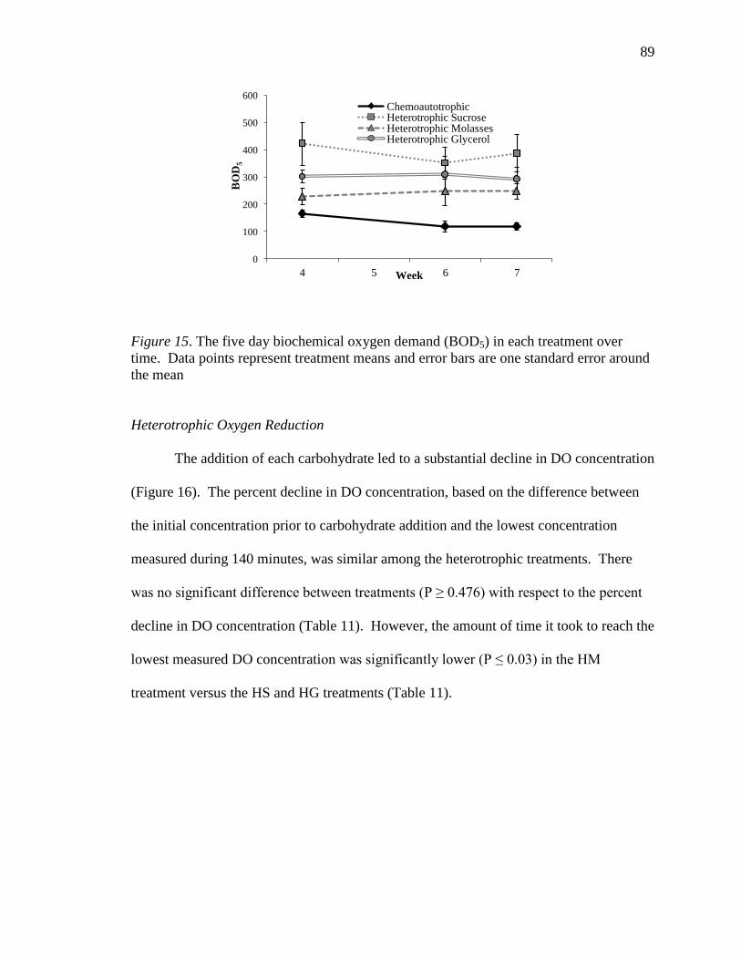
89

Figure 15. The five day biochemical oxygen demand (BOD5) in each treatment over

time. Data points represent treatment means and error bars are one standard error around

the mean

Heterotrophic Oxygen Reduction

The addition of each carbohydrate led to a substantial decline in DO concentration

(Figure 16). The percent decline in DO concentration, based on the difference between

the initial concentration prior to carbohydrate addition and the lowest concentration

measured during 140 minutes, was similar among the heterotrophic treatments. There

was no significant difference between treatments (P ≥ 0.476) with respect to the percent

decline in DO concentration (Table 11). However, the amount of time it took to reach the

lowest measured DO concentration was significantly lower (P ≤ 0.03) in the HM

treatment versus the HS and HG treatments (Table 11).

0

100

200

300

400

500

600

4 5 6 7

BO

D5

Week

ChemoautotrophicHeterotrophic SucroseHeterotrophic MolassesHeterotrophic Glycerol

90

Figure 16. Dissolved oxygen concentration in the heterotrophic tanks just before

carbohydrate addition (time 0) and measured every 5 minutes after that addition, up to

140 minutes. Data points represent treatment means and error bars are 1 standard error

around the mean. Each data point is representative of at least 6 observations.

Shrimp Production

Shrimp production was low, possibly due to the cold temperatures during this

study. Weekly mean ± SEM shrimp growth rate was 0.7 ± 0.1 g wk-1

in the CA

treatment, 0.7 ± 0.0 g wk-1

in the HS treatment, 0.2 ± 0.1 g wk-1

in the HM treatment, and

0.6 g wk-1

in the HG treatment. There were no significant differences (P > 0.05) in

5.0

5.5

6.0

6.5

7.0

7.5

8.0

8.5

Dis

solv

ed

Oxyg

en

(m

g L

-1)

5.0

5.5

6.0

6.5

7.0

7.5

8.0

8.5D

isso

lved

Ox

yg

en

(m

g L

-1)

5.0

5.5

6.0

6.5

7.0

7.5

8.0

8.5

0 10 20 30 40 50 60 70 80 90 100 110 120 130 140

Dis

solv

ed

Oxygen

(m

g L

-1)

Time (minutes)

a.

b.

c.

HS

HM

HG

91

growth rate between the CA, HS, or HG treatments, but growth rate in the HM treatment

was significantly (P < 0.05) lower than the CA and HS treatments (Figure 17a).

Figure 17. Mean shrimp growth rate (a) and survival (b) for each treatment:

chemoautotrophic (CA), heterotrophic-sucrose (HS), heterotrophic molasses (HM), and

heterotrophic glycerol (HG). Error bars are 1 standard error around the mean; different

letters signify significant (P < 0.05) differences between treatments.

Mean ± SEM shrimp survival was 45.2 ± 3.6% in the CA treatment, 53.2 ± 8.9%

in the HS treatment, 16.8 ± 6.9% in the HM treatment, and 49.2 ± 7.3% in the HG

treatment (Figure 17b). There were no significant differences (P > 0.05) in survival

between the CA, HS, and HG treatments, but survival was significantly lower (P < 0.05)

in the HM treatment compared to the CA treatment.

0

10

20

30

40

50

60

70

Su

rv

iva

l (%

)

0.0

0.1

0.2

0.3

0.4

0.5

0.6

0.7

0.8

0.9

Gro

wth

Ra

te (

g w

eek

-1)

CA HS HM HG

Treatment

a

ab

b

a

ab

a

b

a

a.

b.

92

Discussion

C:N Ratio

The C:N ratios of the heterotrophic treatments were intentionally maintained at a

level higher than that recommended by Avnimelech (1999). The high ratios were

intended to ensure the domination of heterotrophic bacteria in those systems, and were

comparable to that of Xu and Pan (2012) who used a C:N ratio of 20:1.

The C:N ratios of the HS and HG treatments were similar at 24.4:1 and 23.4:1,

respectively. The HM treatment had a C:N ratio of inputs that was somewhat lower at

20.4:1. This is still well above the published minimum for heterotrophic domination

(Avnimelech, 1999).

Temperature

Low temperature was a problem in this study. Clifford (1985) reported that

temperature in the range of 12-15⁰ C can be lethal to shrimp. During this study morning

water temperatures of 15⁰ C were recorded (Table 10). Nighttime temperatures may have

been lower than this because temperature was not measured until after sunrise. These

low temperatures likely contributed to the relatively low growth rates and the low

survival during the study. The small, 500-L tanks were susceptible to diurnal

temperature swings as well, perhaps further hindering shrimp growth.

Chemoautotrophic (CA) Treatment

There was a small increase in ammonia concentration during week 2 (0.8 mg

TAN L-1

) in the CA treatment. This was no higher than increases found in any other

treatment, but could have caused some mortality. The increase in ammonia followed a

relatively high concentration of nitrite (8.6 mg NO2-N L-1

) during week 1. This

93

concentration is above the safe level (6.1 mg NO2-N L-1

at 15‰ salinity and a pH of 8.0)

recommended by Lin and Chen (2003). There may have been some mortality in CA

tanks during the time that nitrite concentrations were elevated. A spike in nitrite such as

this can be a common occurrence in aquaculture systems that rely on nitrification to cycle

nitrogen (Cheng and Chen 2002; Wang et al. 2004); this is one of the disadvantages of

managing a chemoautotrophically-driven system. Nitrite oxidizing bacteria may be

slower to establish an effective population than ammonia oxidizing bacteria resulting in a

nitrite spike (Browdy et al. 2012).

Nitrate increased substantially in the CA treatment to a peak mean concentration

of 162 mg NO3-N L-1

. This signifies that nitrification proceeded as intended in this

treatment. Although nitrate is much less toxic to shrimp than either ammonia or nitrite,

elevated nitrate concentrations have been shown to hinder L. vannamei survival and

growth (Kuhn et al. 2010). Tsai and Chen (2002) recommended a safe concentration for

the culture of Penaeus monodon to be 145 mg NO3-N L-1

at 15‰ salinity.

Phosphate increased over time in the CA treatment (Figure 12a), which is a

normal finding as phosphorus from feed is continually introduced to the water (ex. Ray et

al. 2010a; Ray et al. 2011b). Alkalinity decreased over time in the CA treatment tanks

(Figure 12b) likely due to the consumption of carbonate by chemoautotrophic bacteria

(Ebeling et al. 2006). Although sodium bicarbonate was added to the CA tanks,

alkalinity was significantly lower in this treatment compared to the heterotrophic

treatments.

Both TSS and VSS were significantly lower in the CA treatment, indicating a

lower concentration of biofloc suspended in the water column of this treatment versus the

94

heterotrophic treatments. The lower concentration of biofloc likely signifies that a lower

abundance of the microbes associated with those particles would be found in CA tanks.

Ray et al. (2010b) found that removing biofloc from culture systems reduced the

abundance of bacteria, cyanobacteria, rotifers, and nematodes. A lower abundance of

such organisms, all of which consume oxygen in the dark, may be a contributing factor to

the lower BOD5 in the CA treatment. The mean concentration of settleable solids was

lower in the CA treatment than the other treatments, although there were no significant

differences between any of the treatments (Table 11). The high level of variability in

settleable solids measurements likely prevented the detection of significant differences

between treatments. It is unclear what led to this variability; however, notable

differences in the buoyancy of particles were observed. These differences in buoyancy

did not seem to correspond to particular treatments, and may have contributed to the

variability.

Turbidity was significantly lower in the CA treatment compared to the HS and

HG treatments; however, no significant difference was found between the CA and HM

treatments. Correlations between turbidity and suspended solids are rare because

characteristics of particles such as shape and size affect the turbidity measurement

(APHA 2005). Although there were no statistical relationships between treatments with

respect to settleable solids concentrations, the CA and HM treatments had similar mean

concentrations at 37 and 47 ml L-1

, respectively (Table 11). The weight of particles,

measured as TSS, was different between CA and HM treatments, but the turbidity and

settling solids concentrations were similar. This may indicate that although the weight of

95

solids was different, some physical characteristics of the solids in these two treatments

were similar.

The fact that BOD5 was significantly lower in the CA treatment compared to the

other treatments indicates that microbial respiration was lower in the CA treatment. In

intensive biofloc systems the oxygen demand of the microbial community contained in

the water column can at times equal that of the cultured animals (Browdy et al. 2012).

Injection of pure oxygen to overcome these oxygen demands can represent a substantial

operating cost. Therefore, managing the microbial community in a fashion that consumes

less oxygen, such as the CA treatment in this case, may present an economical advantage.

Heterotrophic Treatments

Each of the heterotrophic treatments had an increase of ammonia and nitrite

concentrations during week 1 of the study (Figure 11). During this time ammonia

concentration was greatest in the HS treatment, followed by the HM treatment, and lastly

the HG treatment. The concentration of nitrite was similar among all of the heterotrophic

treatments during this time. This increase in inorganic nitrogen compounds may be

indicative of an establishment period for heterotrophic bacterial function. The water

originally brought into the culture tanks had not received any carbohydrate additions to

stimulate heterotrophic assimilation prior to the beginning of the study. Feed and

carbohydrate additions began when shrimp were placed into the water. The bacterial

community may have taken some time to become established, either in abundance or in

function, when this shift in system management took place. This event may be similar in

causation to that of the spike in nitrite concentration in the CA treatment, where nitrite

oxidizing bacteria did not adequately respond to the increase of nutrient inputs.

96

In subsequent weeks, the concentrations of ammonia and nitrite increased

substantially in the HM treatment (Figure 11). At times there were relatively high

concentrations of ammonia and nitrite simultaneously, posing a potential synergistically

detrimental effect on shrimp.

One of the most discernible differences between the CA treatment and the

heterotrophic treatments was that of nitrate concentration (Figure 11c). Nitrate was either

very low or below detection most of the time in the heterotrophic treatments. This

signifies that the dominant nitrogen pathway in those treatments was not nitrification. It

is possible that some photosynthetic assimilation of nitrogen occurred in the treatments

designed to be heterotrophic. However, Brune et al. (2003) indicated that high-rate algal

assimilation could account for 10-12 g C removal m-2

day-1

, after which systems should

shift to bacterial domination (Avnimelech 1999). The heterotrophic systems in this study

received between 34 and 40 g of C m-2

day-1

on average. Furthermore, there were no

signs of algal proliferation or function in the heterotrophic treatments. Water in the HM

treatment appeared dark brown, and water in the HS and HG treatments had a light brown

appearance. The DO concentrations and pH values were consistently lower in the

afternoon than the morning in the heterotrophic treatments (Table 10), which suggests net

cellular respiration.

While phosphate concentration increased over time in the CA treatment, it

decreased slightly in the heterotrophic treatments (Figure 12a). Initial phosphate

concentration was 29.6 mg PO4 L-1

, and the final mean phosphate concentrations were

21.1, 25.5, and 20.9 mg PO4 L-1

in the HS, HM, and HG treatments, respectively. This

may be due to assimilation of phosphate by heterotrophic bacteria (Longnecker et al.

97

2010; Zubkov et al. 2007). Phosphate was measured during this study as dissolved

orthophosphate which readily binds to particles such as biofloc (Teichert-Coddington et

al. 1999). The heterotrophic treatments had significantly higher biofloc concentrations

(Table 11), which may have helped to remove dissolved phosphate from the water.

Furthermore, removing biofloc with settling chambers has been shown to lower dissolved

phosphate concentrations (Ray et al. 2010a), and a greater amount of biofloc was

removed from the heterotrophic tanks in this study (Table 11).

Typically heterotrophic nitrogen assimilation results in reduced alkalinity because

bicarbonate is used as a carbon source during the process (Ebeling et al. 2006). However,

in the current study alkalinity concentration increased in the heterotrophic treatments.

During week 2, alkalinity concentrations generally leveled-off in the heterotrophic

treatments, and shortly thereafter began to increase (Figure 12). Week 2 was also the

time that settling chambers were first used to remove biofloc from the tanks. Regression

analyses indicated that there was an inverse relationship between VSS and alkalinity in

each treatment. Ray et al. (2011b) saw increased alkalinity being returned from settling

chambers. In the current study alkalinity concentration in the water returning from

settling chambers was not measured. One potential explanation for increased alkalinity

in heterotrophic treatments is that denitrification, which typically generates alkalinity,

may have been occurring in the settling chambers. However, in the heterotrophic

treatments of the current study and in one of the treatments described by Ray et al.

(2011b) there was little or no nitrate detected. Nitrate is the thermodynamically superior

electron acceptor for the denitrification process (van Rijn et al. 2006). It is possible that

98

denitrification was occurring in the two studies but electron acceptors other than nitrate

such as nitrite or nitrous oxide were being utilized by denitrifying bacteria.

The significantly higher concentrations of TSS and VSS in the heterotrophic

treatments versus the CA treatment signify that biofloc concentration was higher in the

heterotrophic treatments. Ebeling et al. (2006) indicated that heterotrophic bacterial

assimilation can generate 40 times the amount of solids compared to chemoautotrophic

nitrification for each unit of ammonia processed. Generating more solids can be a

negative attribute of systems managed to be dominated by heterotrophic bacteria. The

concentration of solids in the water must be managed to optimize shrimp production (Ray

et al. 2010a; 2011b). Relatively more solids in a culture system should result in a greater

amount of solids removal. In the current study both the HS and HG treatments had

significantly more solids removed through settling chambers than the other treatments

(Table 11). Although more material was also removed from the HM settling chambers

than the CA chambers on average, this difference was not significant. However, a low

probability value (P = 0.09) suggests that the difference between these two treatments

may be substantially large.

The BOD5 was significantly higher in the HS and HG treatments versus the HM

treatment. The BOD5 in HS, HG, and HM treatments were significantly greater than in

the CA treatment (Table 11). This indicates that microbial respiration and oxidative

processes consumed a greater amount of oxygen in the heterotrophic treatments versus

the chemoautotrophic treatment. This may translate to higher operating costs for

heterotrophic systems, especially if the injection of pure oxygen gas is required (Browdy

et al. 2012). The HM treatment had a lower BOD5 than the other heterotrophic

99

treatments, and the microbial community in the HM treatment seemed to respond to

carbohydrate inputs differently than the HS and HG treatments. This was evident from

the significantly faster drop in DO concentration in the HM treatment versus the HS and

HG treatments (Table 11). Although the DO concentration dropped to its lowest level at

a higher rate in the HM treatment, the amount of decline in the DO concentration was

similar among each of the heterotrophic treatments. The addition of each carbohydrate

caused an approximately 28% drop in DO concentration. Although DO concentration in

the HM treatment dropped quickly, it seemed to recover somewhat during the 140 minute

observation time (Figure 16b). DO concentrations in the HS treatment showed a slight

increase after reaching the lowest levels following carbohydrate addition (Figure 16a),

but the HG treatment showed no substantial signs of recovery in DO concentration

(Figure 16c). When carbohydrates are added, microbial oxygen consumption can create

dangerously low DO concentrations. Therefore, it is important to understand how

carbohydrate additions can affect DO concentration.

Shrimp Production

Mean shrimp growth rate was 0.7 g wk-1

in the CA and HS treatments, 0.6 g wk-1

in the HG treatment, and 0.2 g wk-1

in the HM treatment. Survival was 45, 53, 49, and

17% in the CA, HS, HG, and HM treatments, respectively. The relatively slow growth

rates and low survival of the CA, HS, and HG treatments may have been caused by

fluctuations of inorganic nitrogen concentrations (especially during the first 2 weeks) and

the unfavorable temperatures recorded during the study. Venero et al. (2009) reported a

study conducted in a commercial scale biofloc culture system during which shrimp

growth rate was similar, at 0.9 g wk-1

and survival was 60%. It is possible that shrimp

100

grown at high density in small tanks do not perform well. In 6,200-L tanks Ray et al.

(2010a) reported growth rates between 0.6-0.9 g wk-1

. Growing shrimp in 500-L tanks at

the same stocking density as the current study but with 100% daily water exchange and

temperature between 25 and 30° C, Suárez et al. (2009) obtained a growth rate of 0.9 g

wk-1

.

Both growth rate and survival were unacceptably low in the HM treatment. High

ammonia concentrations in the HM treatment may have contributed to the poor shrimp

production. Also, the rapid drops in DO concentration after molasses addition may have

led to some undetected lethal DO concentrations. The rapid DO concentration drop also

may have stressed the shrimp, potentially contributing to poor production. Furthermore,

the low concentration of carbon in molasses implies that there is a higher concentration of

unusable components in this carbohydrate source. Components other than carbon may

foul the water and give it the dark brown color observed.

Shrimp production was similar among the HS, HG, and CA treatments suggesting

the potential equivalency of these management strategies. The addition of carbohydrates,

increased oxygen demand, and larger volume of solids generated in the heterotrophic

treatments represent costs of operation that were not factors in the chemoautotrophic

treatment. The results of this study indicate that managing biofloc systems to function in

a chemoautotrophic fashion may be superior to heterotrophic function.

101

CHAPTER V

COMPARING SALINITIES OF 10, 20, AND 30‰ IN MINIMAL-EXCHANGE,

INTENSIVE, BIOFLOC-BASED SHRIMP (LITOPENAEUS VANNAMEI) CULTURE

SYSTEMS

Introduction

Minimal-exchange, intensive, biofloc-based systems undergo low rates of water

exchange. This feature greatly enhances biosecurity, reduces or eliminates pollution

from effluent, and may facilitate inland culture of marine animals. These systems are

stocked at high animal densities which reduces the area needed to culture animals and

makes indoor, temperature controlled production possible. As a result of low water

exchange, high stocking densities, and the use of only crude solids management, a dense

microbial community develops in the water column. This microbial community is

responsible for cycling nutrients, some of which are potentially toxic to shrimp. The

microbial community, partially contained on flocculated (biofloc) particles may also

provide nutrition to shrimp, thereby helping to recycle expensive nutrients from feed

(Burford et al. 2004; Moss 1995; Wasielesky et al. 2006).

These systems can be sited away from the coast, using less expensive land and in

close proximity to urban areas. Many urban areas have a high demand for quality, fresh

shrimp which can be sold at premium prices (Browdy and Moss 2005). Even with

minimal-exchange systems some water must be replaced as a result of solids

concentration management and, with reuse between culture cycles, some water may need

to be replaced due to the accumulation of contaminants such as metals. Considering this

water use in addition to the initial filling of production systems, the cost of artificial sea

102

salts or imported seawater can be a substantial expense at inland facilities. Therefore,

shrimp production systems should be operated at the lowest salinity possible to optimize

financial returns.

The isosmotic point for L. vannamei is reported to be 24.7‰ salinity (Castile and

Lawrence 1981). At this salinity shrimp should not have to spend energy osmoregulating

to maintain a stable haemolymph osmolality. At lower salinities L. vannamei typically

has to hyperosmoregulate, a function performed partially by the renal organ and antennal

gland, but to the largest extent by the gills (Roy et al. 2010).

There are conflicting reports as to whether L. vannamei growth rates are

compromised at salinities below the isosmotic point. Bray et al. (1994) found no

significant difference in shrimp growth between animals grown in 5 and 15‰ salinity

and no significant difference in growth between shrimp grown in 25 and 35‰ salinity.

However, the shrimp cultured in the two lower salinities grew significantly faster than

those at the two higher salinities. This is in contrast to a more recent study by Yan et al.

(2007) who found that as salinity was increased from 11 to 21 to 31‰, there was a

significant increasing trend in shrimp growth rate. Neither study found significant

differences in shrimp survival among these salinities.

In the United States, L. vannamei are currently being produced at salinities of 1-

15‰ in Alabama, Arizona, Florida, and Texas (Roy et al. 2010). However, these are

relatively low intensity operations, stocking shrimp at roughly 10 to 40 m-3

in outdoor

ponds. There is a lack of information on low or moderate salinity marine shrimp culture

using minimal-exchange, intensive biofloc technology. Operating low salinity minimal-

exchange, intensive biofloc systems will likely pose unique challenges due to the

103

common fluctuations in concentration of inorganic nitrogen compounds (Browdy et al.

2012). The toxicity of inorganic nitrogen compounds, including ammonia, nitrite, and

nitrate, have inverse relationships with salinity (Schuler et al. 2010; Kuhn et al. 2010).

The ionic composition of saltwater can vary based on its source (Roy et al. 2010).

The concentration and ratios of a few major seawater ions are most important for L.

vannamei culture. Saoud et al. (2003) demonstrated that potassium, magnesium, and

sulfate were all positively correlated with shrimp survival. Roy et al. (2007) found that

decreasing the sodium: potassium ratio increased shrimp growth and survival. They also

demonstrated that low concentrations of magnesium resulted in higher shrimp respiration

and low survival rates. Roy et al. (2007) recommended maintaining a Na:K ratio

approximately equal to that of seawater (28:1) and a Mg:Ca ratio of 3.1:1.

The purpose of this study was to compare water quality, system function, and

shrimp production dynamics in commercial-scale, biofloc-based culture systems operated

at three different salinities (10, 20, and 30‰).

Methods

Shrimp Source, Nursery, and Feeds

Eight-day postlarvae (PL 8) Litopenaeus vannamei were obtained from Shrimp

Improvement Systems, LLC (Islamorada, Florida, USA). These shrimp were stocked in a

nursery raceway at a density of 4000 shrimp m-3

. The nursery raceway was 3.2 m x 30.1

m x 0.52 m (W x L x D), constructed of cement blocks filled with steel-reinforced

cement, and lined with HDPE. All raceways used for this study were located under

dome-shaped greenhouse structures which were covered in two layers of clear plastic.

The nursery raceway contained a central wall made of plastic sheeting and suspended

104

from the greenhouse cross beams; water was propelled around this wall using 6 airlift

mechanisms described by Ray et al. (2011b) and Ray (2012). Each airlift mechanism

consisted of three, 15.2 cm long ceramic air diffusers oriented parallel to the water flow

and receiving air from a 746 W regenerative blower (Sweetwater®, Aquatic Ecosystems

Inc., Apopka, Florida, USA). The airlifts were constructed of a 2.5 cm diameter PVC

frame which held the diffusers approximately 6 cm above the raceway floor. Above the

diffusers was a sheet of EPDM rubber held by the PVC frame and oriented at an

approximately 35° angle relative to the water movement. Air from the diffusers traveled

vertically and contacted the EPDM, which served as a deflector to project the air and the

water traveling with it horizontally forward.

The nursery raceway was operated at a salinity of 25‰ and shrimp were grown in

the nursery for 54 days. Sucrose was added periodically to raise the C:N ratio and

stimulate heterotrophic bacterial assimilation of ammonia. However, ammonia

concentration was found to be dangerously high (> 5 mg TAN L-1

) and water exchanges

were conducted on 4 occasions to offset these high levels. Throughout the nursery phase

a total volume of water was exchanged equivalent to 140% of the system volume.

For the first 16 days of the nursery shrimp were fed freshly hatched Artemia sp.

(INVE Aquaculture, Inc., Salt Lake City, Utah, USA) at a rate of 500,000 Artemia sp. L-1

day-1

. Next, a series of Zeigler feeds (Zeigler™ Brothers Inc., Gardners, Pennsylvania,

USA) were applied in the nurseries; the guaranteed analysis information for these diets

was provided by the manufacturer. On the first day, 600 mL of Zeigler EZ Larva (250-

400 µm) was added to each nursery, and 300 mL was added on the second day. The

Zeigler EZ Larva diet had a guaranteed analysis of 11.0% crude protein, 6.0 % crude fat,

105

1.0% crude fiber, and 70.0% moisture. On days 1 through 22 Zeigler PL Raceway Plus

400-600 µm diet was added to the nurseries; on days 9 through 34 Zeigler PL Raceway

Plus 600-850 µm diet was added; on days 15 through 54 Zeigler PL Raceway Plus 850-

1200 µm diet was added. Each of the Zeigler PL Raceway Plus diets had a guaranteed

analysis of 50.0% crude protein, 15.0% crude fat, 1.0% crude fiber, 10.0% moisture, and

7.5% ash. On days 23 through 54, Zeigler PL 40-9 Vpak 1.5 mm diet was provided to

the nurseries. This diet had a guaranteed analysis of 40% crude protein, 9% crude fat,

3% fiber, 10% moisture, and 13% ash. On days 34 through 54, Zeigler Hyperintensive-

35 Extra Short 2.4 mm diet was provided. This diet had a guaranteed analysis of 35%

crude protein, 7% crude fat, 2% crude fiber, 12% moisture, and 15% ash. During the

nurseries shrimp were fed based on a percent of the assumed shrimp biomass, starting at

15% of biomass and gradually decreasing to 8.8%.

Experimental Systems and Design

At the end of the nursery phase, shrimp were sampled using the methods

described by Ray et al. (2011a) and found to weigh 1.22 ± 0.02 g (mean ± SEM). At this

time, shrimp were enumerated by weight and 12,500 shrimp were placed into each of 9

raceways. These raceways were identical to that used for the nursery phase, except that

only 4 airlift mechanisms were contained in each raceway, a 560 W water pump at each

raceway helped to circulate and aerate the water, and the raceways were filled only to a

depth of 0.26 m (25 m3 volume). The water pump was connected to a 5 cm diameter pipe

that circumvented each raceway. At 10 locations throughout each raceway (Figure 18) a

1.3 cm diameter pipe connected Venturi nozzles (Turbo-Venturi®, Kent Marine, Franklin,

Wisconsin, USA) to the 5 cm diameter pipe. Each Venturi was located just below the 5

106

cm diameter pipe. Connected to the outflow of the Venturi was 1.3 cm diameter piping

that extended down to approximately 3 cm above the bottom of the raceway before

turning 90 degrees and extending 14 cm parallel to the bottom of the raceway. Each

Venturi had tubing attached to the gas injection point which then attached to another

pipe, 2.5 cm in diameter that circumvented the raceway. This pipe had two valves to

allow ambient air to be drawn in and a point where pure oxygen gas could be injected,

allowing air, pure oxygen, or a combination of the two to be injected into the raceway

water through the Venturi nozzles.

Figure 18. The configuration of the 9 experimental raceways used for this study.

The 5 cm diameter water pipe that circumvented each raceway supplied water to 4

spray bars. Spray bars were 1.3 cm diameter pipes with 2, 2 mm diameter holes drilled in

them, and the spray bars were located just behind the airlift mechanisms (Figure 18).

Venturi

Nozzle

Corner

Board

Spray

Bar

Water

Flow

Air

Lift

107

Water coming from the holes in the spray bars contacted the surface water of the raceway

on either side of the airlifts because previous experiments had shown that foam and

floating microbial mats tended to accumulate in these areas otherwise. The 5 cm

diameter water pipe also supplied water to a 1.9 cm pipe that carried water to the settling

chambers at each raceway.

This experiment was conducted during winter months at the University of

Southern Mississippi’s Thad Cochran Marine Aquaculture Center (CMAC), a part of the

Gulf Coast Research Laboratory, located in Ocean Springs, Mississippi, USA. To control

temperature a centralized heating system, consisting of two hot water boilers connected

to heat exchangers located in each raceway, was utilized. The two 500,000 BTU boilers

(RBI, Division of Mestek Canada, Inc., Ontario, Canada) heated fresh, clean water to 66⁰

C. This water was continuously pumped through a central line that passed near each

raceway. Adjacent to each raceway was a digital controller that received a signal from a

temperature probe submerged in the raceway. The controller operated a small pump that,

when turned on, opened a check valve and sent hot water from the central line through a

3.7 m long, 8 bar, titanium heat exchanger located in each raceway. Digital controllers

could be set to maintain the desired temperature in each raceway.

An 8-day “rest” period was initiated after moving the shrimp to the experimental

raceways, allowing shrimp to recover from any stress incurred during stocking. During

this time the shrimp were kept in 25 m3

of 25‰ salinity water, and temperature was

maintained at 24⁰C initially, and gradually increased to 28⁰C. The 9 raceways were each

randomly assigned to 1 of 3 treatments: a low salinity treatment at 10‰ salinity (LS), a

medium salinity treatment at 20‰ (MS), and a high salinity treatment at 30‰ (HS).

108

After the 8-day rest period, clean water was slowly added to the raceways to bring

them to the correct salinity and depth. Salinity was measured using a YSI Model 556

Handheld Instrument (YSI Incorporated, Yellow Springs, Ohio, USA) which measures

conductivity and temperature to calculate salinity. Water at a salinity of approximately

20‰ was obtained from Davis Bayou, a tributary of The Mississippi Sound adjacent to

the CMAC in Ocean Springs, Mississippi, USA. This water was bleached, aerated, and

dechlorinated with sodium thiosulfate. Salinity was increased to approximately 35‰

using Fritz Super Salt Concentrate (Fritz Pet Products, Mesquite, Texas, USA) and

sodium chloride (Morton® Purex

® Salt, Morton

® Salt, Chicago, Illinois, USA). Municipal

water was used as a source of fresh water. Combinations of fresh and salt water were

used to reach the desired salinity in each raceway based on assigned treatments. This

process was carried out over an additional 8 days, after which 50 shrimp from each

raceway were weighed in groups of 10 to estimate mean individual shrimp weight and the

experiment began; this was considered time point 0.

Water Quality

At time point 0, when the experiment began, water samples were collected and

filtered with 0.7 µm pore size filters for Na, Mg, K, and Ca concentration analysis. These

samples were sent to the Clemson Agricultural Services Laboratory (Clemson, South

Carolina, USA) for analysis using inductively coupled plasma mass spectrometry.


(DO), pH, and salinity in the raceways were measured using the YSI Model 556

Handheld Instrument. Ammonia, nitrite, alkalinity, total suspended solids (TSS), volatile

suspended solids (VSS), turbidity, and settleable solids were measured in each

109

experimental raceway once per week. At time point 0, week 4, and week 8 nitrate

concentration was measured in each raceway. Phosphate (orthophosphate) concentration

was measured at weeks 1, 2, 4, and 6. Five-day biochemical oxygen demand (BOD5)

was measured at weeks 2 through 6, and chlorophyll-a concentration was measured at

weeks 0, 3, 4, 7, and 8. Raceway water samples were collected approximately 4 cm

below the water surface, near the intake of the pumps that distributed water around the

raceways and to the settling chambers.

Ammonia (TAN) was assessed using Hach method 8155 (Hach Company 2003)

and nitrite (NO2-N) was measured using the spectrophotometric procedure outlined by

Strickland and Parsons (1972). Absorbance was measured at 655 nm for TAN and 543

nm for NO2-N using a Hach DR 3800 spectrophotometer (Hach Company, Loveland,

Colorado, USA). The concentration of NO2-N plus NO3-N was determined using the

chemiluminescence detection method described by Braman and Hendrix (1989); NO3-N

was calculated by subtracting NO2-N concentration. The concentration of PO4 was

measured using the PhosVer 3 (ascorbic acid) method outlined in Hach Method 8048

(Hach Company 2003) and absorbance was measured at 890 nm using the Hach DR 3800

spectrophotometer. Alkalinity was measured following the Potentiometric Titration to

Preselected pH procedure outlined in section 2320 B by the APHA (2005). BOD5 was

measured using the procedure described in section 5210 B by the APHA (2005), which

includes a 5 day incubation period at 20⁰ C. Chlorophyll-a extraction was performed

according to the methods described by DeLorenzo et al. (2004) using a combination of

acetone submersion and freezing. Absorbance was measured using the Hach DR 3800 at

664, 665, and 750 nm. Absorbance at 665 and 750 nm was remeasured following

110

addition of 1.0 M hydrochloric acid. Concentrations of chlorophyll-a were calculated

using equations given in section 10200 H by APHA (2005). TSS and VSS concentrations

were measured following ESS Method 340.2 (ESS 1993). Turbidity was measured in

Nephelometric Turbidity Units (NTU) using a Micro 100 Turbidimeter (HF Scientific,

Fort Myers, Florida, USA). Settleable solids was measured by allowing solids to settle

for one hour in an Imhoff cone, as described in Section 2540 F (APHA 2005).

Systems Management

After checking salinity in all raceways each morning, those raceways that were

farthest above the intended salinity due to evaporation received fresh water. The

objective was to keep the water in each raceway within 0.5‰ salinity of the target value

for each treatment. A 2 m3 tank was filled with municipal water, dechorinated using

sodium thiosulfate, aerated, and tested for chlorine prior to use. Water was pumped to

raceways that needed it; this process was repeated 1-4 times per day.

The morning pH readings were used to decide how much sodium bicarbonate to

add to each raceway every day. If the pH in a raceway was above 7.9 no NaHCO3 was

added; if the pH was less than 7.9 but greater than 7.7, 300 g of NaHCO3 was added; if

the pH was less than 7.7 but greater than 7.5, 500 g of NaHCO3 was added; if the pH was

less than 7.5, 1,000 g of NaHCO3 was added.

Sucrose (Extra Fine Granulated Cane Sugar, Sysco® Corporation, Houston, TX,

USA) was added to each raceway three times per day between feedings and through the

night on 12 hour belt feeders to facilitate heterotrophic bacterial assimilation of inorganic

nitrogen. The wet weight of feed added daily was multiplied by 50% to determine the

amount of sucrose to add each day based on the protocol applied in Chapter II. When

111

concentrations of ammonia and nitrite were high, additional sucrose was added. Overall,

the amount of sucrose added was 57.4% of the wet weight of the feed resulting in a C:N

ratio of inputs of 10.9:1.

Each raceway was equipped with a 760 L settling chamber described in Chapter

II. The pump that helped to circulate water in each raceway also delivered water to the

respective settling chamber. Water flowed back from each chamber by gravity. Based

on the findings in Chapter II, the settling chambers in this study were operated at a flow

rate of 15 LPM. Water flowed through the settling chambers continuously, with the

exception of the time that settled material was removed from them. Once per week,

water flow was terminated to each settling chamber for approximately one hour to allow

thorough settling of particles in the chamber. A small submersible pump with a short

hose attached was lowered into the top of the settling chambers to decant the water back

to each raceway and leave the settled material. As the pump was lowered, the color of

the water being pumped to the raceway was monitored. When the pump was lowered to

the point of returning settled material, signified by a much darker color, the pump was

lifted just above that point and allowed to pump all of the relatively clear water back to

the raceway. The settled material on the bottom of the chamber was then drained.

Shrimp Culture

For the first 9 days after shrimp were moved to the growout raceways, both the

Zeigler PL 40-9 Vpak diet and the Zeigler Hyperintensive-35 diet were provided, after

which only Zeigler Hyperintensive-35 diet was given. Equal portions of feed were

broadcast evenly through each raceway by hand 4 times per day at 0730, 1000, 1230,

1500 hrs. At 1630 hr. feed was placed on 2, 12 hour belt feeders at each raceway which

112

constantly delivered feed for 12 hours. Each day 70% of the feed ration was delivered by

hand and 30% was placed on the belt feeders. During the 8 day rest period and the 8 day

salinity adjustment period feed rations were 40% of what they were during the

experiment. During the experiment feed rations were based on routine dip net sampling

for shrimp and uneaten feed in each raceway. Feed rations were adjusted such that no

uneaten feed could be found in the raceways 30 minutes prior to each feeding. Each

raceway received the same amount of feed at every feeding, and each feed portion was

weighed on a digital balance. Shrimp weights were measured once per week by

weighing five groups of ten shrimp from each raceway; these shrimp were collected from

various locations throughout the raceways using a dip net. During this experiment

shrimp were grown for 8 weeks.



cases the range is given in parentheses. The statistical software used for this study was

Systat Version 13 (Systat Software, Inc., Chicago, Illinois, USA).

To compare the concentrations of Na, Mg, K, and Ca, the LS treatment data were

multiplied by 3 and the MS treatment data were multiplied by 1.5. The data were then

compared using a one way ANOVA with salinity as the factor. The concentration of DO,

ammonia, phosphate, alkalinity, BOD5, VSS, settleable solids, and the turbidity data were

analyzed using a fixed model, one-way, repeated measures (RM) ANOVA followed by

pairwise comparisons. Ammonia, VSS, and settleable solids data were log10 transformed

prior to analysis to conform to the assumptions of the ANOVA. Turbidity data were

cosine transformed because this transformation resulted in adherence to the ANOVA

113

assumptions. Morning and afternoon temperature and pH data, salinity, nitrite, nitrate,

chlorophyll-a, and TSS data could not be transformed to fit the ANOVA assumptions,

therefore a nonparametric Wilcoxon signed rank test followed by pairwise comparisons

was used to analyze these data according to the recommendations of Zimmerman and

Zumbo (1993). The percent water exchanged data were arc sine transformed and

analyzed using a one way ANOVA. The amount of seawater used per kg of shrimp,

seawater used per raceway, and the cost of artificial salt for each treatment were all

analyzed using a one way ANOVA. Shrimp mean weekly growth rate, FCR, final

weight, biomass, and survival were all analyzed using a one way ANOVA.

Results

During week 4 of this study a water pipe on one of the HS raceways broke which

resulted in the raceway being drained, killing all the shrimp in that raceway. No data

from this raceway are included in the results.

During the last week of the study, one of the vertical water pipes in a LS raceway

was removed in an attempt to clear blockage at the last Venturi in the water line. When

this occurred a large amount of thick, dark, sludge-like material poured out of the water

line and into the raceway. Later that day many dead shrimp were found in this raceway,

and a 5% water exchange was performed using clean 10‰ salinity artificial seawater

made in the manner described above. The following day ammonia concentration was 2.0

mg TAN L-1

and nitrite was 3.5 mg NO2-N L-1

. This raceway was, therefore, harvested

on the third day following the disturbance which was 3 days before the others in the

study. A total of 1366 dead shrimp, weighing 17.40 kg, were removed from the raceway

over the course of three days; the remainder of the shrimp were living at the time of

114

harvest. All water quality data from this raceway are included, aside from the last week.

All shrimp production data are included in the reported results. Shrimp production data

from this raceway include only those shrimp that were alive at the time of final harvest

because these were the only shrimp fit for human consumption.

The initial concentrations of some major cations indicate that the salinities of 10,

20, and 30‰ were generally reflected proportionately in the concentration of these ions

(Table 12). When the LS data were multiplied by 3 and the MS data were multiplied by

1.5, for equal comparison, there were significant differences (P = 0.04) between LS and

HS potassium and calcium values. Multiplied in this fashion, the mean potassium value

for the LS treatment was 354 mg L-1

and that of the HS treatment was 335 mg L-1

. The

mean calcium value for the LS treatment was 312 mg L-1

and that of the HS treatment

was 331 mg L-1

.

Table 12.

The initial concentrations of some major cations. Concentrations are reported in mg L-1

as mean ± SEM. Different superscript letters indicate significant differences between

treatments when low salinity values are multiplied by 3 and medium salinity data are

multiplied by 1.5 for comparison.

Temperature was maintained at approximately 29⁰ C (Table 13) with little

variability (Figure 19) using the centralized heating system. There were significant

Treatment

Low S alin ity Med iu m S alin ity Hig h S alin ity

Na+

2873 ± 61 5617 ± 122 8236 ± 82

Mg2+

339 ± 3 673 ± 7 1006 ± 6

K+ 118 ± 1a 230 ± 3ab 335 ± 3b

Ca 2+ 104 ± 1a 210 ± 2ab 331 ± 1b

115

differences in temperature between the treatments for both morning and afternoon

measurements (P ≤ 0.01): MS > LS > HS.

Table 13.

The water quality parameters during the 8 week shrimp production experiment. Data are

presented as mean ± SEM (range), and different superscript letters in a row indicate

significant differences (P ≤ 0.05).

TreatmentLow Salinity Medium Salinity High Salinity

Temperature (⁰C)

AM 29.0 ± 0.0 (26.5 - 29.6)a

29.1 ± 0.0 (26.3 - 29.6)b

28.8 ± 0.1 (26.1 - 29.5)c

PM 29.1 ± 0.0 (27.6 - 30.1)a

29.2 ± 0.0 (27.7 - 30.0)b

29.0 ± 0.0 (27.5 - 30.0)c


)

AM 8.6 ± 0.1 (6.7 - 11.1)a

8.7 ± 0.1 (6.6 - 12.5)b

8.9 ± 0.1 (6.0 - 12.9)c

PM 7.9 ± 0.1 (5.8 - 10.8)a

7.7 ± 0.1 (5.2 - 10.0)b

8.0 ± 0.1 (4.5 - 15.0)a

pH

AM 7.9 ± 0.0 (7.7 - 8.2)a

7.8 ± 0.0 (7.6 - 8.0)b

7.7 ± 0.0 (7.4 - 8.0)c

PM 7.9 ± 0.0 (7.1 - 8.3)a

7.7 ± 0.0 (7.4 - 8.2)b

7.7 ± 0.0 (7.3 - 8.1)c

Salinity (‰) 10.3 ± 0.0 (9.2 - 11.0)a

20.2 ± 0.0 (18.2 - 21.2)b

30.2 ± 0.0 (27.1 - 31.9)c

Ammonia (mg TAN L-1) 0.8 ± 0.2 (0.0 - 4.0) 1.2 ± 0.4 (0.0 - 8.0) 0.7 ± 0.3 (0.0 - 4.4)

Nitrite (mg NO2-N L-1) 0.3 ± 0.1 (0.0 - 3.4)

a0.4 ± 0.2 (0.0 - 3.5)

ab0.6 ± 0.2 (0.0 - 3.3)

b

Nitrate (mg NO3-N L-1) 1.4 ± 1.0 (0.0 - 8.7) 0.3 ± 0.2 (0.0 - 2.0) 0.6 ± 0.3 (0.0 - 1.5)

Phosphate (mg PO4 L-1) 2.4 ± 0.3 (0.6 - 3.8) 2.6 ± 0.3 (1.4 - 4.4) 2.0 ± 0.2 (0.8 - 3.3)

Alkalinity (mg CaCO3 L-1) 310 ± 15 (207 - 442) 320 ± 19 (200 - 509) 322 ± 25 (205 - 500)

BOD5 (mg BOD5 L-1) 180 ± 12 (72 - 243) 164 ± 9 (87 - 211) 171 ± 17 (65 - 238)

Chlorophyll-a (µg L-1) 80 ± 16 (24 - 200) 85 ± 18 (24 - 240) 84 ± 16 (40 - 240)

TSS (mg L-1) 263 ± 14 (185 - 500)

a286 ± 19 (175 - 510)

a330 ± 30 (210 - 645)

b

VSS (mg L-1) 198 ± 14 (95 - 460) 189 ± (35 - 370) 191 ± 24 (90 - 490)

Turbidity (NTU) 74 ± 7 (49 - 211) 64 ± 4 (35 - 126) 61 ± 6 (41 - 127)

Settleable Solids (ml L-1) 7 ± 1 (3 - 18)

a9 ± 1 (4 - 21)

ab9 ± 1 (4 - 21)

b

116

Figure 19. The mean morning (a) and afternoon (b) water temperature in the raceways.

Dissolved oxygen (DO) was maintained at relatively consistent morning and

afternoon concentrations (Figure 20). There were significant differences among

treatments with respect to morning DO concentration (P ≤ 0.02): HS > MS > LS. With

respect to afternoon DO concentration there were significant differences between the LS

and MS treatments and between the HS and MS treatments (P ≤ 0.01): HS, LS > MS

(Table 13).

26

27

28

29

30

Tem

per

atu

re (⁰C

)

LS

MS

HS

26

27

28

29

30

0 1 2 3 4 5 6 7 8

Tem

per

atu

re (⁰C

)

Week

AM

PM

a.

b.

117

Figure 20. The mean morning (a) and afternoon (b) dissolved oxygen concentrations in

the raceways.

The pH was significantly higher in the LS treatment, followed by the MS

treatment, and then the HS treatment (P ≤ 0.01). Morning pH was relatively consistent

throughout the study; afternoon pH was less consistent (Figure 21).

0

2

4

6

8

10

12

0 1 2 3 4 5 6 7 8

Dis

solv

ed O

xy

gen

(m

g L

-1)

Week

0

2

4

6

8

10

12

Dis

solv

ed O

xygen

(m

g L

-1)

LS

MS

HS

a.

b.

AM

PM

118

Figure 21. The mean morning (a) and afternoon (b) pH in the raceways.

Salinity in the raceways was maintained at a consistent level throughout the study

(Figure 22) and was significantly different between treatments (P = 0.000).

Figure 22. The mean salinity throughout the study.

7.4

7.5

7.6

7.7

7.8

7.9

8.0

8.1

8.2

8.3

pH

LS MS HS

7.4

7.5

7.6

7.7

7.8

7.9

8.0

8.1

8.2

8.3

0 1 2 3 4 5 6 7 8

pH

Week

AM

PM

a.

b.

0

5

10

15

20

25

30

0 1 2 3 4 5 6 7 8

Sa

lin

ity

(‰

)

Week

LS MS HS

119

The concentration of ammonia increased substantially in all raceways with the

exception of one raceway belonging to the HS treatment during week 5 of the study

(Figure 23a) which never had a measured ammonia concentration above 0.4 mg TAN L-1

.

One of the MS raceways contained a high concentration of ammonia the following week

(8.0 mg TAN L-1

). Ammonia concentration increased again in most raceways the last

week of the experiment (Figure 23a). There were no significant differences (P > 0.05) in

ammonia concentrations between treatments (Table 13). Nitrite concentration increased

to 1.4 and 1.5 mg NO2-N L-1

in the two HS raceways that remained during week 6.

Nitrite rose again in all but 1 LS and 1 MS raceway during the last week of the study

(Figure 23b). Nitrite concentration was significantly greater in the HS treatment versus

the LS treatment (P = 0.04) and there were no significant differences between the MS

treatment and the other treatments (Table 13). Nitrate concentration was generally low

during this study; one notable exception was that an LS raceway had a concentration of

8.7 mg NO3-N L-1

on the last sample date (Figure 23c). There were no significant

differences (P > 0.05) in nitrate concentration between treatments.

120

Figure 23. The concentrations of ammonia (a), nitrite (b), and nitrate (c) during the 8

week study. Data points are treatment means and error bars are 1 standard error around

the mean.

The concentration of TSS was significantly higher in the HS treatment versus the

LS and MS treatments (P ≤ 0.05): HS > MS, LS (Table 13). Over the course of the first

two weeks, TSS concentration decreased substantially in the raceways (Figure 24a). This

time period likely affected the results of the RM ANOVA; however, after this time, there

appeared to be very little difference in TSS concentration between treatments. There

0

1

2

3

4

5

6

7

mg

TA

N L

-1

0.0

0.5

1.0

1.5

2.0

2.5

3.0

3.5

mg N

O2-N

L-1

LS MS HS

0

1

2

3

4

5

6

7

0 1 2 3 4 5 6 7 8

mg

NO

3-N

L-1

Week

c.

b.

a.

121

were no significant differences between treatments with respect to the concentration of

VSS (Figure 24b).

122

Figure 24. The concentrations of total suspended solids (a), volatile suspended solids (b),

and settleable solids (c), as well as turbidity (d) over the 8 week experiment. Data points

are treatment means and error bars are 1 standard error around the mean.

0

100

200

300

400

500

600

mg

TS

S L

-1

0

100

200

300

400

500m

g V

SS

L-1

LS MS HS

0

5

10

15

20

Sett

lea

ble

So

lid

s (m

l L

-1)

0

20

40

60

80

100

120

140

160

180

200

0 1 2 3 4 5 6 7 8

Tu

rb

idit

y (N

TU

)

Week

d.

c.

b.

a.

123

The concentration of settleable solids was significantly greater (P = 0.03) in the

HS treatment compared to the LS treatment (Table 13) and there were no significant

differences (P > 0.05) between the MS treatment and any other treatment (Figure 24c).

There were no significant differences between treatments with respect to turbidity (Figure

24d).

There were no significant differences (P > 0.05) between treatments in terms of

the BOD5 (Table 13). The BOD5 increased between weeks 3 and 5, followed by a sharp

decrease in week 6 (Figure 25a). The concentration of chlorophyll-a was approximately

200 µg L-1

just prior to the beginning of the study but decreased to approximately 50 µg

L-1

by week 3 (Figure 25b). There were no significant differences (P > 0.05) in

chlorophyll-a concentration between treatments.

Figure 25. The BOD5 (a) and chlorophyll-a (b) concentrations during the study. Data

points are treatment means and error bars are 1 standard error around the mean.

0

50

100

150

200

250

0 1 2 3 4 5 6 7 8

Ch

loro

ph

yll

-a (

µg

L-1

)

Week

LS MS HS

50

100

150

200

250

BO

D5

(mg B

OD

L-1

)

b.

a.

124

The volume of material removed with the settling chambers was replaced with

clean water, constituting the only water exchange implemented for this study; the only

exception being the water exchanged just before harvesting the LS raceway that was

harvested early. This water exchange was not considered in the following calculations

because it was performed during the last two days of shrimp culture in 1 raceway.

The mean amount of full salinity seawater (35‰) used per kg of shrimp produced

in the LS, MS, and HS treatments was 104, 159, and 235 L kg-1

, respectively (Table 14);

these amounts were significantly different between the three treatments (P ≤ 0.02). There

were no significant differences between treatments (P > 0.05) with respect to the volume

of water exchanged. The estimated cost of artificial sea salts based on those currently

used at the CMAC to make one full raceway of water was significantly higher (P =

0.000) in the HS treatment, followed by the MS treatment, and then the LS treatment

(Table 14). These results suggest that the cost of salt would be 4.37, 6.91, and 10.26

USD kg-1

shrimp in the LS, MS, and HS treatments, respectively.

Table 14.

The amounts of full strength (35‰) seawater used per raceway, total water exchanged,

and the cost of using artificial sea salt mixed with fresh water to fill the volume of one

raceway used for this study. Data are presented as mean ± SEM, different superscript

letters in a row indicate significant (P ≤ 0.02) differences between treatments.

*Cost of artificial sea salt does not include the cost of fresh water. Cost is based on using one 36 kg bag of Morton brand NaCl

(Morton® Purex® Salt, Morton® Salt, Chicago, Illinois, USA) and one 19-L bucket of Fritz brand Super Salt Concentrate (Fritz Pet

Products, Mesquite, Texas, USA) to make each 1,514-L of 35‰ water.

Treatment

LS MS HS

Total 35‰ Seawater Used per Raceway (m3) 15.0 ± 0.1

a29.8 ± 0.0

b45.1 ± 0.0

c

35‰ Seawater Used per kg Shrimp (L kg-1

) 104 ± 14a

159 ± 5b

235 ± 4c

Total Water Exchange (%) 5.0 ± 0.3 4.5 ± 0.1 5.2 ± 0.0

Cost of Artifical Sea Salt per Raceway (USD)* 653.8 ± 2.2a

1,300 ± 0.7b

1,964 ± 0.2c

125

Because of the mortality event that occurred in one of the LS raceways, the

shrimp production in that treatment was poor compared to the others (Table 15).

However, there were no significant differences (P > 0.05) in any shrimp production

metrics between treatments. Growth rate (Figure 26) was high and feed conversion ratio

(FCR) was low (Table 15). At the time of harvest, all shrimp, including those in the

problematic raceway, were of high quality. Shrimp had full, long antennae, firm

exoskeletons, and almost no lesions in the exoskeletons.

Table 15.

Shrimp production in the three treatments. Data are presented as mean ± SEM, there

were no significant differences between the treatments with respect to any of these

parameters.

Figure 26. Shrimp weight throughout the 8 week production study. Data points are

treatment means and error bars are 1 standard error around the mean.

Treatment

LS MS HS

Growth Rate (g week-1

) 1.8 ± 0.1 2.0 ± 0.0 2.0 ± 0.1

FCR 1.6 ± 0.2 1.2 ± 0.0 1.2 ± 0.0

Mean Weight (g) 17.8 ± 0.9 19.3 ± 0.2 19.0 ± 0.5

Biomass (kg) 149.5 ± 19.2 188.2 ± 5.7 191.5 ± 3.5

Biomass volume-1

(kg m-3

) 3.0 ± 0.4 3.8 ± 0.1 3.8 ± 0.1

Survival (%) 68 ± 10 78 ± 2 81 ± 1

0

2

4

6

8

10

12

14

16

18

20

0 1 2 3 4 5 6 7 8

Wei

gh

t (g

)

Week

LS MS HS

126

Discussion

Significant differences in initial potassium and calcium between the LS and HS

treatments when the LS values were multiplied by 3 may indicate that the concentrations

of these two elements were not proportionate to the intended salinities of 10 and 30‰.

The LS treatment potassium value was 6% lower than the HS treatment, and the LS

treatment calcium value was 6% higher than that of the HS treatment. A difference of

6% is likely not a biologically significant difference. Furthermore, the ratios that Roy et

al. (2007) determined to be biologically important for shrimp were similar between

treatments. Using mean values from Table 12, the Na:K ratios were 24.3:1, 24.4:1, and

24.6:1 in the LS, MS, and HS treatments, respectively. The Mg:Ca ratios were 3.3:1,

3.2:1, and 3.0:1 in the LS, MS, and HS treatments, respectively. The Na:K ratios were

lower than the 28:1 ratio recommended by Roy et al. (2007). However, according to

those authors a lower ratio is preferable to a higher ratio. The Mg:Ca ratios were similar

to the ratio of 3.1:1 recommended by Roy et al. (2007).

The water temperature during this study was adequately regulated by the central

heating system. This is in contrast to daily temperature fluctuations experienced during

shrimp production in the summer months, as in Chapter II. The significant differences in

temperature between treatments were likely caused by the location of raceways with

respect to the hot water delivery system. Those raceways farthest from the boilers tended

to be slightly cooler. However, the maximum mean differences of 0.3⁰ C are likely not

biologically significant to shrimp or the microbial community in the water column.

The concentration of DO during this study was also relatively consistent. The DO

concentration was maintained at a high level to ensure that this was not a source of stress

127

for shrimp. In commercial operations the high concentrations used for this study may not

be desirable due to the cost associated with oxygen injection. Raceways probably

received different amounts of oxygen. This may have contributed to the significant

differences in DO concentrations between treatments. Although these differences

existed, DO concentration was always sufficient to allow survival and growth in each

treatment. Because no significant differences were found in BOD5 concentrations, it is

not likely that substantial differences in microbial respiration existed between treatments.

The intensive monitoring of pH and salinity and the regular inputs of sodium

bicarbonate and fresh water resulted in consistent pH and salinity during this study. The

consistency in temperature, DO, pH, and salinity during this study may have contributed

to the high shrimp production values obtained, as a more constant physical environment

can help to minimize stress for aquatic animals (Stickney 2005).

The cause of the inverse relationship between pH and salinity in this study is

unclear. In seawater pH typically increases with higher salinity because more carbonate

and bicarbonate ions are present with higher salinity, contributing to a higher pH

buffering capacity (Libes 2009). Saraswat et al. (2011) found that in both laboratory and

estuarine experiments, as salinity increased so did pH. However, in a study similar to the

current project, Decamp et al. (2003) cultured L. vannamei in minimal-exchange biofloc

systems with treatments of 9, 18, and 36‰ salinities, and found that pH was significantly

lower as salinity increased. These authors attributed the relationship between salinity and

pH to potentially increased photosynthesis in the lower salinity treatments. This may

have been the case in the current study as well, although photosynthetic oxygen

production was not measured. Because no significant difference in the chlorophyll-a

128

concentration was found, there probably was not a substantial difference in algal

abundance; however, the taxonomic composition of algae may have differed among

treatments. Higher concentrations of the weak acid CO2 may have been present as

salinity increased, possibly due to increased shrimp respiration. However, the DO and

BOD5 concentrations seem to contradict the idea of increased respiration.

There are chemical and physical relationships between temperature, pH,

alkalinity, CO2, and salinity (APHA 2005). Temperature and salinity both have inverse

relationships with the concentration of CO2, although temperature has a much greater

impact. The pH of water has an inverse relationship with CO2, and alkalinity has a

positive relationship with CO2 concentration. Each of these parameters, aside from

salinity which has the least effect, is in favor of an increasing dissolved CO2

concentration and decreasing pH with increasing salinity. Carbon dioxide dynamics may

be further justified as a cause of decreased pH by examining the morning versus

afternoon pH readings (Table 13 and Figure 21). The afternoon pH values are generally

lower than morning values and much more variable over time. This may be an indication

of the relatively higher CO2 generation during the day when feed and sucrose inputs were

greatest and respiration rates may have been higher. Also, the DO concentrations were

substantially lower in the afternoon (Table 13), further indicating relatively higher

respiration rates during the day.

The ammonia spike during week 5 (Figure 23a) of the study was followed by a

sharp decline in BOD5 concentration the following week (Figure 25a). It is unusual that

the BOD5 decline did not correspond to a drop in DO or an increase of pH, suggesting

that the BOD5 measurement during week 6 may have been incorrect. However, the

129

BOD5 drop, if it is accurate, may have been an indication that a portion of the microbial

community died, and the decomposition of those microbes could have contributed to

increased ammonia concentrations. Nitrite and nitrate concentrations began to increase at

approximately the same time as ammonia (Figure 23b, c), potentially signifying the

oxidation of ammonia and nitrite by nitrifying bacteria. It is unclear why these increases

of inorganic nitrogen compounds occurred, as sucrose was added multiple times per day

to facilitate heterotrophic assimilation of nitrogen.

At week 0, chlorophyll-a concentration was much higher than after the study

started (Figure 25b). This is likely a result of the shift from systems with relatively

abundant algae to systems more dominated by heterotrophic bacteria after the intensive

additions of feed and sucrose began. Such a shift in microbial dominance also was noted

by Browdy et al. (2001). The mean chlorophyll-a concentrations reported in the current

study are approximately 15% of what was reported by Ray et al. (In Press) and 20% of

that reported by Venero et al. (2009); both groups of authors operated biofloc systems

with no supplemental carbohydrate additions. However, the chlorophyll-a concentrations

reported here are more than 5 times higher than what was reported by Moreno-Ostos et

al. (2008) in oligotrophic waters.

The concentration of TSS was most divergent between treatments and highest at

time point 0 (Figure 24a). It is unclear why this is the case, but TSS concentrations in

general may have been influenced by the differences in salinity during this study. There

were significant differences in TSS, but not in VSS. The VSS data represents the filtered

organic matter that is burned at 550⁰ C and does not include the weight of minerals which

do not combust. Therefore, in this case where salinity is different between treatments,

130

VSS concentration is likely the best indicator of the weight of biofloc particles in the

water column. Furthermore, finding no significant differences between treatments in

turbidity is an indication that optical clarity was not substantially different. Settleable

solids was significantly higher in the HS treatment compared to the LS treatment;

however, considering the large overlap in ranges between treatments (Table 13) this

difference may not have been significant in terms of system function.

Table 14 helps to illustrate the substantial savings in seawater use by considering

the culture of marine shrimp at lower salinities. At inland aquaculture facilities, these

water savings translate directly to cost savings when considering the price of artificial sea

salts. The low rate of water exchange during this study (Table 14) also helps to lower

seawater use and justify inland shrimp aquaculture. Water was exchanged only as a

result of solids removal. Several similar trials conducted at the Oceanic Institute (OI) in

Hawaii, USA were reported to have used 187, 172, and 402 liters of seawater per kg of

shrimp (Otoshi et al. 2007).

The stocking density of shrimp in this intensive production study is lower than

those densities reported for superintensive shrimp production. Venero et al. (2009)

reported production trials from OI, Texas Agrilife Research Center in Corpus Christi,

TX, USA, and the Waddell Mariculture Center in Bluffton, SC, USA. In these trials,

shrimp were in life stages similar to the current study, stocking density ranged from 430

shrimp m-3

to 807 shrimp m-3

; growth rates ranged between 0.9 and 1.5 g wk-1

, and

survival ranged from 60 to 91%. The shrimp production results in each of the current

treatments are similar to those reported by Venero et al. (2009). Considering the entire

production cycle, including the time period that temperature and feeding rates were

131

deliberately low, this study was carried out in approximately 10 weeks. The lower

stocking density likely helped to facilitate fast shrimp growth, as shrimp grow faster at

lower densities (Sookying et al. 2011).

Although there were no significant differences in shrimp production between

treatments, the substantially lower production in the LS treatment would translate to less

profit for a commercial shrimp operation. Biomass produced in the LS treatment was

20.6% lower than that of the MS treatment, meaning a proportionally similar decrease in

profit assuming that a similar price is obtained for shrimp from the two treatments as the

LS shrimp were also smaller (Table 15). The estimated cost of artificial salts was 49.7%

lower in the LS treatment compared to the MS treatment. However, in a commercial

shrimp production facility the salt water used to grow shrimp would be saved and used

for multiple shrimp culture cycles.

In summary, the production goals and availability of sea salt should be considered

when deciding the salinity at which to culture shrimp. It is unclear whether the problems

that arose in the low salinity raceway during this study would have occurred if a similar

situation had taken place in a higher salinity system; however, the likelihood would have

been lower. Because of the fluctuations in ammonia and nitrite that are common in

intensive biofloc-based shrimp culture systems the medium salinity of 20‰ is likely the

best choice of the three options explored here. This salinity represents considerable cost

savings over higher salinity, but based on the current results, can result in excellent

shrimp production.

132

CHAPTER VI

CARBON AND NITROGEN STABLE ISOTOPE DYNAMICS IN INTENSIVE,

BIOFLOC-BASED SHRIMP (LITOPENAEUS VANNAMEI) NURSERIES

Introduction

Intensive, biofloc-based shrimp aquaculture systems provide distinct advantages

over extensive systems. Because very little water is exchanged and specific pathogen

free animals are used, the chance of viral pathogen introduction is virtually eliminated.

Reduced water use provides enhanced environmental sustainability and the ability to

culture marine shrimp at inland locations, potentially providing fresh shrimp to

metropolitan markets (Browdy and Moss 2005).

Biofloc-based aquaculture systems do not have substantial mechanical filtration

or external biofilters. Rather, as a result of intensive nutrient inputs through feeds, a

dense microbial community develops in the water column. This microbial community is

partially contained in flocculated, organic (biofloc) particles made up of detritus,

microbial secretions, algae, bacteria, fungi, protists, and zooplankton. The microbial

community is responsible for detoxifying nitrogen compounds, of which ammonia and

nitrite are most toxic. Studies also have demonstrated the enhancement of shrimp growth

in the presence of biofloc particles (Moss 1995; Otoshi et al. 2001; Xu and Pan 2012).

Biofloc-based systems have proven to be effective for the nursery rearing of shrimp from

several day post-larvae to over 1 g, juvenile shrimp (Cohen et al. 2005; Samocha et al.

2007).

The comparison of stable carbon and nitrogen isotope values between consumers

and potential food items is a common ecological procedure to evaluate the contribution of

133

dietary items to animal nutrition (Fry 2006; Gannes et al. 1997). There is an increasing

body of literature on the contributions of natural biota to shrimp in aquaculture systems

using stable isotopes (Burford et al. 2004; Epp et al. 2002; Parker et al. 1989). However,

information is lacking on the specific contributions of feed versus biofloc in shrimp

nursery systems. The purpose of the current study was to evaluate the contribution of

applied feeds and the suspended biofloc community to shrimp carbon and nitrogen needs

during nursery production of juvenile shrimp. Also, the study aimed to investigate

potential interactions between changes in feed, biofloc, and shrimp isotopic levels.

Methods

Shrimp Husbandry

Brood stock shrimp were obtained from the Oceanic Institute (Waimanalo, HI,

USA) and placed into shrimp maturation systems described by Ogle (1992). Shrimp

were matured and spawned according to the procedures described by Ogle (1991).

Shrimp from a total of 6 spawning events were obtained and each of these sets of shrimp

was staggered through larval rearing periods. Post-hatch larval shrimp were fed a

combination of the diatom Chaetoceros gracilis and brine shrimp Artemia sp. during a 20

day larval rearing period. The larval rearing period was conducted in static-water

fiberglass tanks receiving blown air through ceramic diffusers.

As the larval rearing periods ended, these 6 sets of shrimp were stocked into 3

nursery raceways over 14 days. Five-day postlarval shrimp (L. vannamei) were stocked

into the nurseries at densities of 3000, 2700, and 3200 shrimp m-3

in raceways 1, 2, and 3,

respectively. Shrimp were grown in the nurseries for between 46 and 62 days, depending

on when they were initially stocked.

134

The raceways were contained under clear plastic-covered greenhouses and

measured 3.2 x 30.1 x 0.52 m (W x L x D). Approximately 75% of the water used to fill

them was previously bleached water from Davis Bayou, a tributary of The Mississippi

Sound adjacent to the Thad Cochran Marine Aquaculture Center (CMAC) in Ocean

Springs, Mississippi, USA. The remaining 25% of the water in the 50 m3 nurseries was

artificial seawater made with municipal water and a mixture of Fritz Super Salt

Concentrate (Fritz Pet Products, Mesquite, Texas, USA) and sodium chloride (Morton®

Purex®

Salt, Morton®

Salt, Chicago, Illinois, USA). Of the total water volume in each

raceway, 20% was reused from the study described in Chapter II. Water was reused so

that a microbial community would be present from the beginning to help cycle nutrients

and provide nutrition to post-larval shrimp. Salinity was maintained at approximately

25‰ through the periodic addition of fresh municipal water. Water was propelled around

a central wall in each raceway using airlift mechanisms described in Chapter II and by

Ray (2012). Pure oxygen was injected through micro-pore diffusers if dissolved oxygen

concentration was below 4 mg L-1

.

Shrimp were fed a combination of 3 Zeigler PL Raceway plus diets (Zeigler™

Brothers Inc., Gardners, Pennsylvania, USA) with size ranges 400 – 600, 600 – 850, and

850 – 1200 µm. The diets were guaranteed by the manufacturer to contain a minimum of

50% protein and 15% fat, and a maximum of 1% fiber, 12% moisture, and 7.5% ash. The

next feed provided was 1.5 mm, Zeigler PL 40-9: Vpak, which had a manufacturer-

provided guaranteed analysis of a minimum of 40% protein and 9% fat, and a maximum

of 3% fiber, 10% moisture, and 13% ash. Each of the diets was provided to shrimp based

on weekly observations of shrimp size and measurements of weight. Larger sized feeds

135

were applied as shrimp grew and application of different feeds overlapped one another to

account for variability in the size of shrimp. The amount of feed provided was based on

an assumed shrimp biomass calculated using shrimp weights and an estimated mortality

rate of 2% wk-1

. Feeding rate was originally 15% of assumed biomass and gradually

decreased to 9.5% of biomass.

Water Quality


(DO), pH, and salinity in the raceways were measured using a YSI Model 556 Handheld

Instrument (YSI Incorporated, Yellow Springs, Ohio, USA). Ammonia, nitrite, nitrate,

total suspended solids (TSS), volatile suspended solids (VSS), turbidity, and alkalinity

were measured in each raceway once per week. Ammonia (total ammonia nitrogen,

TAN) was assessed using Hach method 8155 (Hach Company 2003) and nitrite (NO2-N)

was measured using the spectrophotometric procedure outlined by Strickland and Parsons

(1972). Ammonia and nitrite were measured more frequently when high concentrations

of these toxic substances were detected. Absorbance was measured at 655 nm for

ammonia and 543 nm for nitrite using a Hach DR 3800 spectrophotometer (Hach

Company, Loveland, Colorado, USA). The concentration of NO2-N plus NO3-N was

determined using the chemiluminescence detection method described by Braman and

Hendrix (1989); NO3-N was calculated by subtracting NO2-N concentration. Both TSS

and VSS were measured using ESS Method 340.2 (ESS 1993). Turbidity was measured

in Nephelometric Turbidity Units (NTU) using a Micro 100 Turbidimeter (HF Scientific,

Fort Myers, Florida, USA). Alkalinity (as CaCO3) was measured using the

136

Potentiometric Titration to Preselected pH procedure outlined in section 2320 B by the

APHA (2005).

When TSS concentrations were above 500 mg L-1

the 760 L settling chambers

described in Chapter II were used to lower TSS. Submersible pumps contained in a wire

frame cage, covered in fine mesh were placed in the raceways and used to pump water to

the settling chambers at a flow rate of approximately 6 LPM. Water flowed back from

the settling chambers to the raceways. Settling chambers were operated until the

following week and their use was discontinued if TSS concentration was below 500 mg

L-1

.

Stable Isotopes

Beginning the fifth week after the first shrimp were stocked in the nurseries, 10

shrimp were collected randomly from each raceway. Beginning the fourth week after the

first shrimp were stocked, 1 L of water was collected from each raceway. During the

weeks that both shrimp and water were collected, the two items were gathered

simultaneously. Both shrimp and water samples were collected during 4 consecutive

weeks. Shrimp were rinsed with deionized water, dried, ground, acid washed with 10%

HCl, rinsed, dried and finely ground and homogenized. Water was centrifuged and the

pellet was acid washed with 10% HCl, rinsed, dried and finely ground and homogenized.

Each of the feeds also were collected, dried and finely ground and homogenized.

Triplicate samples were placed into a Costech Model 4010 Elemental Combustion

System which combusted the samples and supplied gaseous C and N (as CO2 and N2) to a

Thermo, Delta V Advantage Isotope Ratio Mass Spectrometer (Thermo Scientific,

137

Bremen, Germany). The mass spectrometer generated δ 13

C and δ 15

N values, calculated

using the following equation:

(

)

where R = the ratio of heavy over light isotopes, in this case 13

C/12

C or 15

N/14

N. The

standard used for C was Pee Dee Belemnite and that used for N was atmospheric N.

Microbes can assimilate nutrients quickly, and isotope levels in those microbes

can reflect those of the source within two days (Burford et al. 2004). However, more

than one trophic level of organisms inhabit biofloc systems (Ray et al. 2010b), likely

leading to dynamic temporal changes in biofloc isotope levels. Also, it has been shown

that it can take approximately 14 days for post-larval shrimp to reach isotopic equilibrium

with their diet (Al-Maslamani 2006). Considering these issues, the sampling regime

depicted in Figure 27 was used. Data reported from a particular sample number for this

study include the weighted mean of feed isotope values for a full week, biofloc isotope

data collected at the end of that week, and shrimp isotope data from the following week.

This is to allow time for the feed to affect isotope levels of the biofloc, and both the

biofloc and feed to affect isotope levels of the shrimp.

138

Figure 27. A depiction of the way that sampling was staggered to account for the

dynamic changes in biofloc and the length of time needed for shrimp to incorporate

isotopic signatures of their diets.

The shrimp fractionation factors calculated in Chapter III (2.4‰ for δ15

N and

1.3‰ for δ13

C) were subtracted from the measured shrimp isotope values in this study to

account for trophic fractionation between shrimp and their diet.

The following two equations were used to estimate the relative amount of C and

N contributed to shrimp by potential food sources (Fry 2006).

Where is the fraction of C or N contributed by source 1, and is the fraction

contributed by source 2. The sample was shrimp; source 1 was feed and source 2 was

biofloc. The use of these equations assumes that there are only 2 sources of C and N

available to shrimp.

Feed Sampling

(weighted mean δ

values of feeds applied

during this time)

Biofloc Sampling

Shrimp Sampling

7 days 7 days

139

Data Analysis

To determine if relationships existed between parameters measured for this study,

linear regression analysis was performed in multiple instances. The software utilized was

Systat Version 13 (Systat Software, Inc., Chicago, Illinois, USA). The concentration of

VSS was compared to C and N isotope levels of the biofloc using a natural polynomial

regression; in the analysis of VSS versus δ15

N values data were log10 transformed to

satisfy the normality assumption of the test. Ammonia and nitrite concentrations were

compared to δ15

N values of the biofloc using a linear least squares analysis; nitrite

comparison data were log10 and tangent transformed to make the data fit a normal

distribution. Using linear least squares analyses, the concentration of VSS and the mean

weight of shrimp were each compared to the calculated %N contribution from feed to

shrimp, and the feed and biofloc isotope levels were compared to shrimp isotope levels.

Results

Water Quality

Temperature, DO, pH, and salinity (Table 16) were within acceptable ranges for

the growth of L. vannamei (Clifford 1985). The afternoon DO concentration was

occasionally high due to pure oxygen injection. However, the trend in higher mean DO

concentrations and pH levels in the afternoon versus the morning measurements is likely

indicative of algal productivity during the day. Also, higher mean afternoon temperatures

are the result of solar heat input to the raceways throughout the day.

140

Table 16.

The water quality parameters measured in each of the three nursery raceways used for

this study. Data are reported as mean ± SEM (range).

The concentration of ammonia was of concern during this study. When shrimp

sample number 1 was collected ammonia was below detection (BD) (< 0.01 mg TAN L-

1), 2.1, and 2.5 mg TAN L

-1 in the 3 raceways, respectively. At the following sample

point ammonia concentration was BD, 5.1, and 5.3 mg TAN L-1

, respectively; it was 6.4,

0.3, and 0.4 mg TAN L-1

, respectively at the following sample point. During the last

sample time, ammonia was below 1 mg TAN L-1

in all raceways. Table 16 provides

values for ammonia concentrations as well as other water quality constituents over the

entire nursery period, not limited to the time that samples were collected for stable

Raceway

1 2 3

Temperature (⁰C)

AM 29.3 ± 0.1 (27.4 - 30.8) 29.0 ± 0.1 (24.2 - 30.5) 29.6 ± 0.1 (25.8 - 31.1)

PM 30.9 ± 0.1 (29.2 - 32.2) 30.8 ± 0.2 (25.9 - 33.3) 31.6 ± 0.1 (29.7 - 34.0)


)

AM 7.3 ± 0.2 (5.8 - 12.5) 6.7 ± 0.1 (4.9 - 9.2) 6.5 ± 0.1 (4.8 - 9.2)

PM 7.7 ± 0.2 (5.3 - 10.4) 8.0 ± 0.2 (4.8 - 17.9) 7.6 ± 0.2 (5.2 - 14.9)

pH

AM 8.2 ± 0.1 (6.7 - 9.2) 8.3 ± 0.1 (7.0 - 9.5) 8.3 ± 0.1 (7.2 - 9.4)

PM 8.5 ± 0.1 (7.1 - 9.4) 8.5 ± 0.1 (7.3 - 9.8) 8.6 ± 0.1 (7.5 - 9.7)

Salinity (‰) 26.5 ± 0.2 (24.7 - 28.0) 26.4 ± 0.1 (24.9 - 28.2) 27.1 ± 0.1 (25.8 - 28.5)

Ammonia (mg TAN L-1

) 2.9 ± 0.6 (0.0 - 9.2) 1.8 ± (0.0 - 6.9) 2.1 ± 0.5 (0.0 - 6.2)

Nitrite (mg NO2-N L-1

) 1.6 ± 0.4 (0.0 - 8.6) 7.0 ± 1.2 (0.0 - 17.4) 5.4 ± 1.0 (0.0 - 12.2)

Nitrate (mg NO3-N L-1

) 0.0 ± 0.0 (0.0 - 0.1) 0.5 ± 0.3 (0.0 - 1.2) 0.0 ± 0.0 (0.0 - 0.0)

TSS (mg TSS L-1

) 358 ± 56 (115 - 750) 520 ± 49 (220 -710) 374 ± 38 (210 - 595)

VSS (mg VSS L-1

) 343 ± 61 (100 - 750) 439 ± 50 (200 - 665) 369 ± 42 (180 - 585)

Turbidity (NTU) 88 ± 22 (18 - 158) 139 ± 34 (34 - 242) 103 ± 23 (28 - 144)


) 219 ± 18 (153 - 302) 237 ± 11 (174 - 262) 241 ± 9 (216 - 286)

141

isotope analysis. This is to ensure a complete representation of the water quality

conditions that shrimp were exposed to during the study.

Nitrite also became highly concentrated at times during this study. Nitrite

reached the highest concentration in raceway (RW) 1 at the time the 4th

shrimp sample

was collected (8.6 mg NO2-N L-1

) for this study. Nitrite remained between 7.7 and 8.6

mg NO2-N L-1

in that raceway for 7 days. Nitrite reached the highest concentration in

RW 2 (17.4 mg NO2-N L-1

) just after shrimp sample 3 was collected; nitrite was 7.9 mg

NO2-N L-1

or higher for 19 days surrounding this time period. Dead shrimp were found

in RW 2 on the day that nitrite reached the highest concentration; through dip net

sampling it was estimated that approximately 5% of the population died at that time.

Nitrite concentration was highest in RW 3 during the same time period that it was

elevated in RW 2; however, no dead shrimp were found in this raceway. Nitrate did not

accumulate appreciably in the nursery raceways (Table 16).

The concentrations of TSS, VSS, and turbidity levels (Table 16) were at times

higher than what has been recommended for optimal shrimp growth in biofloc culture

systems (Ray et al. 2011b). The concentration of VSS, used to estimate the amount of

organic biofloc particles, tended to increase over time in each of the raceways (Figure

28). Alkalinity (Table 16) remained within an acceptable range for nitrification and

buffering against swings in pH (Browdy et al. 2012).

142

Figure 28. Stable isotope levels in shrimp, biofloc (floc), and feed, as well as the

concentration of volatile suspended solids (VSS) over the four weekly sample collections

times in raceways 1 (a, b), 2 (c, d), and 3 (e, f). Graphs on the left represent δ13

C values

and graphs on the right represent δ15

N values. Feed values are weighted means of the

isotope values of all feeds added during one week, floc values are representative of the

biofloc collected at the end of that week, and shrimp values represent shrimp collected

one week later. VSS concentration was measured when the biofloc was collected, as a

means of estimating the amount of biofloc particles. Shrimp isotope values are corrected

to account for trophic fractionation.

Stable Isotopes

There was a significant inverse polynomial relationship (P = 0.000) between VSS

concentration and the δ13

C values of suspended matter (biofloc) (Figure 29a). There was

150

250

350

450

550

650

5

6

7

8

9

10

1 2 3 4

VS

S (m

g V

SS

L-1)

δ1

5N

Sample Number

150

250

350

450

550

650

-24

-23

-22

-21

-20

-19

1 2 3 4

VS

S (m

g V

SS

L-1)

δ1

3C

Sample Number

150

250

350

450

550

650

-24

-23

-22

-21

-20

-19

VS

S (m

g V

SS

L-1)

δ1

3C

150

250

350

450

550

650

5

6

7

8

9

10

VS

S (m

g V

SS

L-1)

δ1

5N

150

250

350

450

550

650

-24

-23

-22

-21

-20

-19

VS

S (m

g V

SS

L-1)

δ1

3C

Shrimp Floc

Feed VSS

150

250

350

450

550

650

5

6

7

8

9

10

VS

S (m

g V

SS

L-1)

δ1

5N

Shrimp Floc

Feed VSS

a.

e. f.

d.c.

b.

143

a significant positive polynomial relationship (P = 0.000) between VSS concentration and

the δ15

N values of biofloc (Figure 29b).

Figure 29. The VSS concentration versus biofloc δ13

C values (a), and VSS concentration

versus biofloc δ15

N values (b)

There was no significant relationship between the concentration of ammonia and

the δ15

N values of biofloc (P > 0.05). However, there was a significant positive

relationship (P = 0.000) between nitrite concentration and the δ15

N biofloc values (Figure

30).

-24.0

-23.5

-23.0

-22.5

-22.0

-21.5

-21.0

-20.5

Bio

floc δ

13C

4

5

6

7

8

9

10

11

250 350 450 550 650

Bio

flo

c δ

15N

VSS (mg VSS L-1)

y = 0.0.215 ∙ 10-4x2 - 0.026x - 15.656

R2 = 0.715

P = 0.000

a.

b.

y = 0.172 ∙ 10-4x2 - 0.007 + 7.004

R2 = 0.459

P = 0.000

144

Figure 30. The dissolved nitrite concentration versus the δ15

N values of biofloc.

There were no significant relationships between VSS concentration or shrimp

weight versus the %N contribution from feed. There were positive relationships (P =

0.000) between both the feed δ13

C values and the biofloc δ13

C values versus the δ13

C

values of shrimp (Figure 31a, b). There was also a significant positive relationship (P

=0.001) between the δ15

N of feed and that of the shrimp (Figure 31c). Conversely, there

was a significant inverse relationship existed (P =0.001) between biofloc δ15

N values and

those of the shrimp (Figure 31d).

5

6

7

8

9

10

11

0 5 10 15

Bio

flo

c δ

15N

Dissolved Nitrite (mg NO2-N L-1)

y = 0.280x + 6.505

R2 = 0.842

P = 0.000

145

Figure 31. Regression plots of feed δ13

C values (a) and biofloc δ13

C values (b) versus

shrimp δ13

C values, as well as feed δ15

N values (c) and biofloc δ15

N values (d) versus

shrimp δ15

N values. Shrimp isotope levels are corrected to account for trophic

fractionation.

For each sample collected except RW 1 sample 1 and RW 3 sample 3, the δ13

C

values for shrimp were above those for feed and biofloc (Figure 28). This made

calculating estimated %C contributions to shrimp from the feed and biofloc impossible

on all but those two dates because consumers must have isotope values between that of

their potential food sources to perform this calculation. Two sample dates would not be

representative of the study. Also, the fact that shrimp isotope values were higher than

both of their potential food sources most of the time indicates that an error may have

occurred. For these reasons, %C contributions to shrimp from feed and biofloc were not

calculated for any sample date.

7

7.5

8

8.5

9

5 6 7 8 9 10 11

Sh

rim

p

δ1

5N

Biofloc δ15N

7

7.5

8

8.5

9

7 7.5 8 8.5 9 9.5

Sh

rim

p δ

15N

Feed δ15N

-22

-21.5

-21

-20.5

-20

-19.5

-19

-18.5

-22 -21.5 -21 -20.5 -20

Sh

rim

p δ

13C

Feed δ13C

-22

-21.5

-21

-20.5

-20

-19.5

-19

-18.5

-24 -23 -22 -21

Sh

rim

p

δ1

3C

Biofloc δ13C

y = 1.560x + 12.765

R2 = 0.523

P = 0.000

y = -0.158x + 9.290

R2 = 0.324

P = 0.001

y = 0.340x + 5.108

R2 = 0.338

P = 0.001

y = 0.768 – 2.902

R2 = 0.531

P = 0.000

a.

d.c.

b.

146

The δ13

C values for biofloc decreased substantially throughout the study, and the

feed δ13

C values also decreased (Figure 28a, c, e). Aside from a relatively large increase

of the δ13

C value in RW 1 shrimp between sample number 1 and 2, the δ13

C values of

shrimp also tended to decrease throughout the study. Similar to the δ13

C values for the

feed, the δ15

N values for the feed tended to decrease over time (Figure 28b, d, f).

However, unlike δ13

C values of the biofloc, the biofloc δ15

N values had a tendency to

increase over time. The δ15

N values of shrimp were variable between raceways in terms

of changes over time; however, in each instance shrimp δ15

N levels fell between that of

feed and biofloc, making an estimation of the %N contribution of those potential N

sources possible.

The estimated proportion of N in shrimp originating from feed or biofloc was

variable between sample dates and between raceways (Figure 32). On the first sample

date shrimp in each raceway seemed to be obtaining a substantial portion of N from the

biofloc. In raceways 2 and 3, that relatively high N contribution from biofloc continued

until the last sample date, during which the N contribution from biofloc was low in each

raceway. The overall mean ± SEM percent N contribution from feed to shrimp in RW 1

was 66 ± 10% and that of biofloc was 34 ± 10%. In RW 2 the mean contribution of feed

to shrimp N was 50 ± 14% and that of biofloc was 50 ± 14%. In RW 3 the mean

contribution of feed to shrimp N was 52 ± 17% and that of biofloc was 48 ± 17%.

147

Figure 32. The estimated N contribution to shrimp from the applied feed and the

suspended matter (biofloc) in raceways 1 (a), 2 (b), and 3 (c).

Shrimp Production

Survival in RW 1 was 42.4%, survival in RW 2 was 21.8%, and survival in RW 3

was 18.4%. The final mean shrimp weight was 1.27g.

Discussion

The high concentrations of ammonia during this study likely contributed to the

relatively low shrimp survival. Lin and Chen (2001) recommended a 3.55 mg L-1

safe

concentration of TAN at a salinity of 25‰. The ammonia concentration was above this

value in RW 1 for 10 days and for 6 days in both raceway 2 and 3. Nitrite concentration

0

10

20

30

40

50

60

70

80

90

100

Sh

rim

p N

So

urce (

%) RW 2

Feed

Biofloc

0

10

20

30

40

50

60

70

80

90

100

1 2 3 4

Sh

rim

p N

So

urce (

%)

Sample Number

RW 3

0

10

20

30

40

50

60

70

80

90

100

Sh

rim

p N

So

urce (

%) RW 1

a.

b.

c.

148

also may have contributed to low shrimp survival. Nitrite was lowest in RW 1 (Table

16), the raceway with highest shrimp survival.

Similarly, Epp et al. (2002) found that δ13

C values of particulate matter in L.

vannamei culture tanks decreased over time and that δ15

N values in the particulate matter

increased over time (Figure 28). Two likely carbon sources for microbes in these

systems are feed and atmospheric carbon (~ 8‰ δ13

C) incorporated into sugars and lipids

by algae. However, in the current study the δ13

C values of biofloc seem to generally

track those of feed (Figure 28). In contrast, the δ15

N values of the biofloc tended to

increase while those of the feed decreased. The increase of δ15

N values in biofloc may be

the result of a changing microbial community, possibly with an increasing number of

higher trophic-level organisms. As trophic level increases so increases the enrichment of

heavy isotopes. Checkley and Entzeroth (1985) found that copepods can have δ15

N

values enriched by as much as 5.8‰ over a diet of suspended particulate matter. If a

higher abundance of zooplankton such as these had occurred in the biofloc, relative to

other organisms, this may have led to an overall enrichment of 15

N in the biofloc.

However, the decrease in δ13

C biofloc values does not support the occurrence of trophic

enrichment.

The concentration of biofloc tended to increase over the course of the study, as

indicated by increasing VSS concentrations (Figure 28). It is unclear whether or not this

caused the lower biofloc δ13

C and higher δ15

N values, but there was a relationship

between VSS and isotope values (Figure 29). It may be more likely that increased VSS

concentration and the observed changes in biofloc isotope levels are both characteristics

of abundant and dynamic microbial communities. As the systems aged shrimp feeding

149

rates increased and added an increasing amount of C and N. With no water exchange, a

portion of C and N that has been added accumulates in microbes. Biofloc systems are

typically dominated by algae in the beginning and transition to bacterial, heterotrophic-

dominated systems as nutrients accumulate (Browdy et al. 2001).

One of the shifts in microbial composition that may have occurred is the

proliferation of ammonia oxidizing bacteria which oxidize ammonia to nitrite. The

accumulation of nitrite is evidence that these bacteria may have increased in abundance.

The positive relationship between nitrite concentration and the δ15

N values of biofloc

(Figure 30) supports the idea that ammonia oxidizers may have been associated with

changes in biofloc N isotope levels.

There was no detectable relationship between shrimp weight and the %N

contribution from feed or biofloc. This is in contrast to a study by Burford et al. (2004)

who found that of 1, 5, and 9 g shrimp, the 1 g shrimp attained the highest proportion of

nitrogen from suspended particulate matter. However, shrimp in the current study were

much smaller, in the weight range of approximately 1 to1270 mg. Burford et al. (2004)

also found that 9 g shrimp attained a higher portion of N than 1 or 5 g shrimp when

exposed to an approximately 20% greater biofloc concentration. In the current study no

relationship was found between the VSS concentration and the %N contribution from

feed or biofloc to shrimp.

Although it was not possible to calculate %C contributions of feed and biofloc to

shrimp, the feed and biofloc δ13

C values both have positive relationships with δ13

C values

in shrimp (Figure 31a, b). This may be an indication that both feed and biofloc

contributed to the C contained in shrimp. Likewise, the positive relationship that feed

150

δ15

N values have with shrimp δ15

N values may indicate that feed contributed a substantial

portion of N to shrimp. This is in agreement with the estimates made by calculating %N

contribution to shrimp from feed.

The inverse relationship between biofloc δ15

N values and shrimp δ15

N (Figure

31d) values seems to contradict the estimated contribution of biofloc to shrimp N. The

relatively low R2 values of the regression analyses between feed and biofloc δ

15N values

and those of shrimp indicate that feed and biofloc N isotope levels do not explain as

much of the variability in shrimp N isotopes as compared to C contributions to shrimp. It

appears that the strength of the inverse relationship between biofloc δ15

N and shrimp

δ15

N values may be disproportionately affected by 6 observations with biofloc δ15

N

values above 10‰ (Figure 31d). In fact, when these observations are deleted from the

analysis, there is no relationship between biofloc and shrimp δ15

N values (P = 0.208).

These 6 observations were made during the last sample date (Figure 28b, c, e), the time

when estimated shrimp %N contribution from biofloc was lowest in RWs 2 and 3, and

among the lowest in RW 1 (Figure 32). Therefore, it is not surprising that the

observations contribute to a poor relationship between biofloc and shrimp δ15

N values.

The fact that shrimp δ15

N values were between those of the feed and biofloc on every

sample date seems to be a good indication that both feed and biofloc contributed to

shrimp N content.

It is unclear why shrimp δ13

C values were consistently higher than those of feed

and biofloc (Figure 28). It is possible that the degree of trophic 13

C fractionation between

shrimp and their diet was higher in this study than in other studies (Chapter III; Parker et

al. 1989). The 13

C fractionation value of 1.3‰ was used because of the findings in

151

Chapter III. The diets used during this study were similar to those used in Chapter III,

although they contain higher protein levels, and are said by the manufacturer to contain

specialized ingredients for the nutrition of young post-larval and juvenile shrimp.

Anderson et al. (1987) demonstrated that different feed ingredients can result in different

apparent levels of fractionation in the trophic transfer to shrimp. This is largely due to

varying assimilation of feed ingredients by shrimp, and the same holds true for varying

microbial assemblages (Gannes et al. 1997).

The variability of %N contribution from biofloc to shrimp may be somewhat

concerning from a management perspective. When shrimp culture managers decide how

much feed to apply in nursery systems, ideally that feed rate should be linear over time.

However, if shrimp receive varying contributions of nutrients from biofloc, feed rates

may need to be adjusted accordingly.

The estimated contributions of biofloc to the nitrogen contained in shrimp during

this study are relatively high. Because protein is typically the most expensive ingredient

in shrimp diets this could contribute to a substantial savings in feed costs for shrimp

nurseries. In this study shrimp from RW 1 were estimated to have received 34% of N

from biofloc, while RWs 2 and 3 received 52 and 48% respectively. These values fall in

the range of what other researchers have estimated. Parker et al. (1989) estimated that

pond biota contributed approximately 60% of the N found in shrimp. Epp et al. (2002)

estimated that shrimp obtained as much as 31% of N from pond biota, and Burford et al.

(2004) estimated that natural biota contributed between 18 and 29% of shrimp N.

In summary, the results of this study support the use of biofloc-based systems for

the nursery culture of L. vannamei. Post-larval and juvenile shrimp may utilize biofloc as

152

a substantial source of C and N, suggesting that feeding can be reduced in biofloc

systems compared to clear water systems while maintaining superior biosecurity over

extensive systems. The isotopic composition of biofloc was related to the amount of

biofloc, and the N isotopic composition was related to the concentration of dissolved

nitrite. These relationships may be indications of changes in the microbial community.

Due to high concentrations of ammonia and nitrite during this study, alternative biofloc

management strategies should be considered. One such strategy is to elevate the C:N

ratio of inputs to favor heterotrophic bacterial N assimilation over nitrification

(Avnimelech 1999), as nitrification did not function reliably in this case.

153

CHAPTER VII

SUMMARY

The results of Chapter II indicate that controlling the flow rate delivered to simple

settling chambers may be an effective means of regulating the concentration of biofloc

particles. Continuous operation of these devices appears to be advantageous due to the

increased alkalinity and decreased solids and nitrate concentrations returned to the

raceways from them. The two sizes of settling chambers used for this study helped to

maintain similar retention times in those chambers.

The treatment with higher flow rate to larger settling chambers resulted in lower

nitrate and solids concentrations, and higher alkalinity; this treatment also had

significantly improved shrimp production. It seems that this management regime is more

appropriate than one with lower flow rate to smaller sized settling chambers. However,

removing more material will necessitate the disposal or on-site remediation of that

material. The results of this study may be important to consider for shrimp production

results, chemical dynamics, and operational expenses for intensive, minimal-exchange,

biofloc-based shrimp culture systems.

Based on the results of Chapter II, the study described in Chapter III compared

recirculating systems with no biofloc to those with biofloc. Particle concentration was

significantly higher in the biofloc tanks, while solids were removed with external filters

in the clear water tanks. Nitrate was substantially higher in the clear water tanks because

of external nitrifying biofilters, while heterotrophic bacteria apparently assimilated

inorganic nitrogen in the biofloc systems. The external biofilters of the clear water

systems maintained low ammonia and nitrite concentrations in those tanks while these

154

compounds became dangerously concentrated in the biofloc tanks at times, likely

contributing to poor shrimp production in one of those tanks.

Although shrimp production was generally low in this study, the use of clear

water tanks allowed C and N stable isotope fractionation values to be estimated. Using

these fractionation levels, the percent C and N in shrimp contributed from the feed and

the biofloc in the biofloc-based tanks was estimated. The estimated C contribution to

shrimp from feed was 72% and that from biofloc was 28%, while the estimated

contribution of N from feed was 42% and that from biofloc was 59% (rounded values).

These results indicate that biofloc may have contributed substantially to shrimp nutrition,

especially with regard to N which enters the system primarily through expensive proteins

in feed. It is unclear whether clear water or biofloc systems are best for shrimp culture.

Based on this preliminary and somewhat narrow study, toxic nitrogen compounds may be

better controlled in clear water RAS; however, biofloc may contribute to shrimp nutrition

thereby potentially lowering feed costs.

Chapter III also provided a comparison of stable isotope levels in whole shrimp

versus what was found only in the abdominal sections. It was found that both 13

C and

15N were significantly enriched in shrimp abdomens, which may have implications for

comparing the results in this document to those of other studies.

The fourth chapter of this document describes an experiment that evaluated the

use of three carbohydrate sources to promote heterotrophic nitrogen assimilation, and

compared these to systems without carbohydrate addition. Tanks that received molasses

had relatively high concentrations of ammonia. In the chemoautotrophic systems

nitrification apparently proceeded, as evidenced by an accumulation of nitrate; however,

155

this accumulation only occurred after a relatively high spike in nitrite. There was no

appreciable amount of nitrate in the tanks intended to function as heterotrophic systems,

indicating that assimilation was likely the dominant process.

A significantly greater amount of solids was generated in the heterotrophic

systems, and biochemical oxygen demand was higher in those tanks indicating that

microbial respiration was greater. In each of the heterotrophic treatments DO

concentration declined by approximately 28% after the addition of each respective

carbohydrate source. However, DO declined significantly faster in the molasses

treatment, reaching its lowest mean point in 27 minutes while the lowest mean DO

concentrations were measured 47 and 75 minutes after the additions of sucrose and

glycerol, respectively. In all of the treatments there were significant inverse relationships

between VSS concentration and alkalinity, indicating that higher VSS may have led to a

decline in alkalinity.

Shrimp growth rate was slow in this study, likely due to low temperatures.

Shrimp survival also was low; however, both growth rate and survival were much lower

in the molasses treatment than any other treatment.

The results of this study indicate the need to consider solids accumulation and

system oxygen demand when deciding on the management protocol for biofloc systems.

Nitrification can result in spikes of toxic nitrogen compounds, whereas in this case, those

compounds did not become highly concentrated in heterotrophic systems with the

exception of the molasses treatment. The results indicate that molasses may not be a

good choice of carbohydrate source for this type of system management, while sucrose

and glycerol appear to yield similar results.

156

In Chapter V three salinities were used to culture shrimp in large raceways. Most

water quality parameters were remarkably similar between the salinities of 10, 20, and

30‰. Temperature and DO concentration differed between the treatments, but it appears

likely that these subtle differences were due to management issues and probably did not

have any biologically significant effects on shrimp or system performance. The pH was

significantly greater as salinity decreased. It is unclear why this was the case, but may be

at least partly attributable to greater CO2 concentrations at higher salinity. Nitrite

concentrations were higher in the 30‰ salinity treatment compared to the 10‰ salinity

treatment, but these differences were not great and, due to lower toxicity of nitrite at

higher salinity, likely did not affect shrimp.

The cost differences associated with salinity are evident when the price of

artificial sea salts is considered. These differences may have substantial impacts for

inland shrimp farming. Shrimp production was not significantly different between the

salinities used in this study. However, due to the introduction of what was likely

anaerobic sludge into a low salinity raceway, the shrimp production was substantially

lower in the low salinity treatment. This event would likely have been less detrimental in

a higher salinity raceway because the toxicities of ammonia and nitrite are lower with

increased salinity. In the 20‰ and 30‰ salinity treatments shrimp growth rate and FCR

were excellent, likely due to the consistency and near optimal level of environmental

parameters during this study. This study illustrates some of the important issues to

consider when deciding what salinity to operate biofloc systems.

Chapter VI helps to illustrate the usefulness of operating shrimp nurseries as

biofloc systems. The C isotope levels of biofloc were inversely related to VSS

157

concentration, and the N isotope levels of biofloc were positively correlated with VSS

concentration. These results may indicate that the concentration of biofloc particles has

an effect on the isotope ratios found in that material, or the results could indicate a

change over time in isotope levels as the system progresses and biofloc becomes more

concentrated. The concentration of nitrite also was positively correlated with the δ15

N

values of biofloc, possibly indicating a divergence in the microbial community associated

with nitrite concentration.

The δ15

C values of both feed and biofloc were positively related to δ15

C values of

shrimp, indicating that both feed and biofloc may have contributed C to shrimp. The

δ15

N values of feed were positively related to those of shrimp; however, the δ15

N values

of biofloc were inversely related to shrimp δ15

N values. These results seem to indicate

that feed was the main contributor of N to shrimp. However, when the N isotope values

of shrimp, feed, and biofloc are placed into a simple two source mixing model, the

estimated contribution of N to shrimp from biofloc ranged from 34 to 50%. The cause of

an inverse correlation between biofloc and shrimp δ15

N values is unclear, but the mixing

model suggests a substantial contribution of N from biofloc.

Juvenile shrimp in nurseries may be especially well suited to take advantage of

biofloc particles due to their smaller size. However, the estimated C and N contributions

of biofloc to shrimp in this nursery study are similar to those calculated using much

larger shrimp in Chapter III. It may be that shrimp size has little impact on biofloc

utilization as a food source. Nonetheless, because biofloc appears to contribute to shrimp

nutrition during the nursery phase, using this technology may help save on feed cost.

158

There are a wide variety of management issues to consider when operating

intensive, minimal-exchange biofloc-based shrimp culture systems. This technology can

result in greater shrimp production per unit area, limited water use, and enhanced

biosecurity compared to extensive systems. However, the effects of biofloc

concentration, carbohydrate sources used, and salinity are among the issues that must be

considered to optimize production, and ultimately the economic competitiveness of both

nursery and growout shrimp production systems. Considering the rapid expansion of the

shrimp aquaculture industry in response to growing demand for shrimp, intensification

will be necessary. Biofloc-based systems offer a potentially environmentally-sustainable

means of accommodating this intensification. Advances in the reliable operation of

biofloc-based culture systems may therefore contribute to responsible growth in shrimp

aquaculture.

159

REFERENCES

Al-Maslamani IAMJ. 2006. Feeding and nutrition in the marine shrimp Penaeus

semisulcatus. Ph.D. Dissertation. University of Wales, UK.

Alonso-Rodriguez R, Paez-Osuna F. 2003. Nutrients, phytoplankton and harmful algal

blooms in shrimp ponds: A review with special reference to the situation in the

Gulf of California. Aquaculture 219: 317–336.

Anderson RK, Parker PL, Lawrence A. 1987. A 13

C /12

C tracer study of the utilization of

presented feed by a commercially important shrimp Penaeus vannamei in a pond

growout system. Journal of the World Aquaculture Society 18(3): 148-155.

(APHA) American Public Health Association, American Water Works Association, and

Water Pollution Control Association. 2005. Standard Methods for the

Examination of Water and Wastewater. 17th ed. Washington, D.C., USA:

American Public Health Association.

Avnimelech Y. 1999. Carbon/nitrogen ratio as a control element in aquaculture systems.

Aquaculture 176: 227-235.

Avnimelech Y. 2006. Bio-filters. The need for a new comprehensive approach.

Aquacultural Engineering 34: 172-178.

Avnimelech Y. 2012. Biofloc Technology: A Practical Guide Book, 2nd

Ed. Baton

Rouge, Louisiana, USA: World Aquaculture Society.

Beveridge MCM, Phillips MJ, Clarke RM, 1991. A quantitative and qualitative

assessment of wastes from aquatic animal production. In: Brune DE, Tomasso,

JR, editors. Advances in World Aquaculture: Aquaculture and Water Quality, vol.

3. Baton Rouge, LA, USA: World Aquaculture Society. p 506–533.

160

Braman RS, Hendrix SA. 1989. Nanogram nitrite and nitrate determination in

environmental and biological materials by vanadium (III) reduction with

chemiluminescence detection. Analytical Chemistry 61: 2715-2718.

Bray WA, Lawrence AL, Leung-Trujillo JR. 1994. The effect of salinity on growth and

survival of Penaeus vannamei, with observations on the interaction of IHHN virus

and salinity. Aquaculture 122: 133-146.

Browdy CL, Bratvold D, Stokes AD, McIntosh RP. 2001. Perspectives on the application

of closed shrimp culture systems. In: Browdy CL, Jory DE, editors. The New

Wave, Proceedings of the Special Session on Sustainable Shrimp Culture. Baton

Rouge, LA, USA: The World Aquaculture Society. p 20-34.

Browdy CL, Moss SM. 2005. Shrimp culture in urban, super-intensive closed systems.

In: Costa Pierce B, Desbonnet A, Edwards P, Baker D, editors. Urban

Aquaculture. Oxfordshire, UK: CABI. p 173-186.

Browdy CL, Ray AJ, Leffler JW, Avnimelech Y. 2012. Biofloc-based aquaculture

systems. In: Tidwell JH, editor. Aquaculture Production Technologies. Oxford,

UK: Wiley-Blackwell. p 278-307.

Brune DE, Schwartz G, Eversole AG, Collier JA, Schwedler TE. 2003. Intensification

of pond aquaculture and high rate photosynthetic systems. Aquacultural

Engineering 28: 65–86.

Burford MA, Thompson PJ, McIntosh RP, Bauman RH, Pearson DC. 2004. The

contribution of flocculated material to shrimp (Litopenaeus vannamei) nutrition in

a high-intensity, zero-exchange system. Aquaculture 232: 525-537.

161

Castille FL, Lawrence AL. 1981. The effect of salinity on the osmotic, sodium and

chloride concentrations in the hemolymph of euryhaline shrimp of the genus

Penaeus. Comparative Biochemistry and Physiology 68A: 75-80.

Chapman PM, Popham JD, Griffin J, Leslie D, Michaelson J. 1987. Differentiation of

physical from chemical toxicity in solid waste fish bioassay. Water Air and Soil

Pollution. 33: 295–309.

Checkley DM, Entzeroth LC. 1985. Elemental and isotopic fractionation of carbon and

nitrogen by marine, planktonic copepods and implications to the marine nitrogen

cycle. Journal of Plankton Research 7(4): 553-568.

Cheng SY, Chen JC. 2002. Study on the oxyhemocyanin, deoxyhemocyanin, oxygen

affinity and acid-base balance of Marsupenaeus japonicus following exposure to

combined elevated nitrite and nitrate. Aquatic Toxicology 61: 181-193.

Clifford HC. 1985. Semi-intensive shrimp farming. In: Chamberlain GA, Haby MH,

Miget RJ, editors. Texas Shrimp Farming Manual. Corpus Christi, Texas, USA:

Texas Agricultural Extension Service. p IV15–IV42.

Cohen JM, Samocha TM, Fox JM, Gandy RL, Lawrence AL. 2005. Characterization of

water quality factors during intensive raceway production of juvenile Litopenaeus

vannamei using limited discharge and biosecure management tools. Aquacultural

Engineering 32: 425-442.

Crab R, Avnimelech Y, Defoirdt T, Bossier P, Verstraete W. 2007. Nitrogen removal

techniques in aquaculture for a sustainable production. Aquaculture 270: 1–14.

Crab R, Chielens B, Wille M, Bossier P, Verstraete W. 2010a. The effect of different

carbon sources on the nutritional value of bioflocs, a feed for Macrobrachium

162

rosenbergii postlarvae. Aquaculture Research 41: 559-567.

Crab R, Lambert A, Defoirdt T, Bossier P, Verstraete W. 2010b. The application of

bioflocs technology to protect brine shrimp (Artemia franciscana) from

pathogenic Vibrio harveyi. Journal of Applied Microbiology 109(5): 1643-1649.

Decamp O, Cody J, Conquest L, Delanoy G, Tacon AGJ. 2003. Effect of salinity on

natural community and production of Litopenaeus vannamei (Boone), within

experimental zero-water exchange culture systems. Aquaculture Research 34:

345-355.

DeLorenzo ME, Leatherbury M, Weiner JA, Lewitus AJ, Fulton MH. 2004.

Physiological factors contributing to the species-specific sensitivity of four

estuarine microalgal species exposed to the herbicide atrazine. Aquatic Ecosystem

Health & Management 7(1): 137-146.

De Schryver P, Crab R, Defoirdt T, Boon N, Verstraete W. 2008. The basics of bio-flocs

technology: The added value for aquaculture. Aquaculture 277: 125-137.

De Schryver P, Boon N, Verstraete W, Bossier P. 2012. The biology and biotechnology

behind bioflocs. In: Avnimelech Y, editor. Biofloc Technology: A Practical Guide

Book, 2nd

Edition. Baton Rouge, LA, USA: The World Aquaculture Society. p

199-215.

Dufault RJ, Korkmaz A, Ward B. 2001. Potential of biosolids from shrimp aquaculture as

a fertilizer for broccoli production. Compost Science & Utilization 9(2): 107-114.

Ebeling JM, Timmons MB, Bisogni JJ. 2006. Engineering analysis of the stoichiometry

of photoautotrophic, autotrophic, and heterotrophic removal of ammonia–nitrogen

in aquaculture systems. Aquaculture 257: 346–358.

163

Emerenciano M, Ballester ELC, Cavalli RO, Wasielesky W. 2012. Biofloc technology

application as a food source in a limited water exchange nursery system for pink

shrimp Farfantepenaeus brasiliensis (Latreille, 1817). Aquaculture Research 43:

447-457.

Epp MA, Ziemann DA, Schell DM. 2002. Carbon and nitrogen dynamics in zero-water

exchange shrimp culture as indicated by stable isotope tracers. Aquaculture

Research 33: 839-846.

(ESS) Environmental Sciences Section, Inorganic Chemistry Unit, Wisconsin State Lab

of Hygiene. 1993. ESS Method 340.2: Total Suspended Solids, Mass Balance

(Dried at 103–105 °C) Volatile Suspended Solids (Ignited at 550 °C). Madison,

WI, USA: Wisconsin State Lab of Hygiene.

FAO (Food and Agriculture Organization of the United Nations). 2007. The state of

world fisheries and aquaculture 2006. Rome, Italy: FAO Fisheries and

Aquaculture Department.

FAO (Food and Agriculture Organization of the United Nations) [Internet]. Fisheries and

aquaculture online statistical database; 2010 [cited 2012 September 6]. Available

from: http://www.fao.org/fishery/statistics/en

Focken U, Groth A, Coloso RM, Becker K. 1998. Contribution of natural food and

supplemental feed to the gut content of Penaeus monodon Fabricius in a semi-

intensive pond system in the Philippines. Aquaculture 164: 105-116.

Fry B. 2006. Stable isotope ecology. New York, USA: Springer.

Gamboa-Delgado J, LeVay L. 2009. Natural stable isotopes as indicators of the relative

contribution of soy protein and fish meal to tissue growth in Pacific white shrimp

164

(Litopenaeus vannamei) fed compound diets. Aquaculture 291: 115-123.

Gamboa-Delgado J., Peña-Rodríguez A., Ricque-Marie D., Cruz-Suárez LE. 2011.

Assessment of nutrient allocation and metabolic turnover rate in Pacific white

shrimp Litopenaeus vannamei co-fed live macroalgae Ulva clathrata and inert

feed: dual stable isotope analysis. Journal of Shellfish Research 30(3): 969-978.

Gannes LZ, O’Brien DM, Del Rio CM. 1997. Stable isotopes in animal ecology:

assumptions, caveats, and a call for more laboratory experiments. Ecology 78(4):

1271-1276.

Hach Company. 2003. Method 8155, Salicylate Method (Ammonia), Method 8048

Phosphorus Reactive (Orthophosphate). Loveland, CO, USA: Hach Company.

Hamlin HJ, Michaels JT, Beaulaton CM, Graham WF, Dutt W, Steinbach P, Losordo

TM, Schrader KK, Main KL. 2008. Comparing denitrification rates and carbon

sources in commercial scale upflow denitrification biological filters in

aquaculture. Aquacultural Engineering 38: 79-92.

Hannouche A, Chebbo G, Ruban G, Tassin B, Lemaire BJ, Joannis C. 2011. Relationship

between turbidity and total suspended solids concentration within a combined

sewer system. Water Science and Technology 64(12): 2445-2452.

Hargreaves JA. 2006. Photosynthetic suspended-growth systems in aquaculture.

Aquacultural Engineering 34: 344–363.

Hari B, Kurup BM, Varghese JT, Schrama JW, Verdegem MCJ. 2004. Effects of

carbohydrate addition on production in extensive shrimp culture systems.


Hopkins SJ, Sandifer PA, DeVoe RM, Holland FA, Browdy CL, Stokes AD. 1995.

Environmental impacts of shrimp farming with special reference to the situation

165

in the continental United States. Estuaries 18 (1A): 25-42.

Jiang DH, Lawrence AL, Neill WH, Gong H. 2000. Effects of temperature and salinity

on nitrogenous excretion by Litopenaeus vannamei juveniles. Journal of

Experimental Marine Biology and Ecology 253: 193-209.

Ju ZY, Forster IP, Dominy WG. 2009. Effects of supplementing two species of marine

algae or their fractions to a formulated diet on growth, survival and composition

of shrimp (Litopenaeus vannamei). Aquaculture 292: 237-243.

Kent M, Browdy CL, Leffler JW. 2011. Consumption and digestion of suspended

microbes by juvenile Pacific white shrimp Litopenaeus vannamei. Aquaculture

319: 363-368.

Kuhn DD, Boardman GD, Lawrence AL, Marsh L, Flick GJ. 2009. Microbial floc meal

as a replacement ingredient for fish meal and soybean protein in shrimp feed.


Kuhn DD, Smith SA, Boardman GD, Angier MW, Marsh L, Flick GJ. 2010. Chronic

toxicity of nitrate to Pacific white shrimp, Litopenaeus vannamei: Impacts on

survival, growth, antennae length, and pathology. Aquaculture 309: 109-114.

Libes SM. 2009. Introduction to marine biogeochemistry, 2nd

Ed. Burlington, MA, USA:

Academic Press, Elsevier.

Li E, Chen L, Zeng C, Chen X, Yu N, Lai Q, Qin JG. 2007. Growth, body composition,

respiration and ambient ammonia nitrogen tolerance of the juvenile white shrimp,

Litopenaeus vannamei, at different salinities. Aquaculture 265: 385-390.

Li E, Xiong Z, Chen L, Zeng C, Li K. 2008. Acute toxicity of boron to juvenile white

shrimp, Litopenaeus vannamei, at two salinities. Aquaculture 278: 175-178.

166

Lin YC, Chen JC. 2001. Acute toxicity of ammonia on Litopenaeus vannamei Boone

juveniles at different salinity levels. Journal of Experimental Marine Biology and

Ecology 259: 109-119.

Lin YC, Chen JC. 2003. Acute toxicity of nitrite on Litopenaeus vannamei (Boone)

juveniles at different salinity levels. Aquaculture 224: 193-201.

Longnecker K, Lomas MW, Van Mooy BAS. 2010. Abundance and diversity of

heterotrophic bacterial cells assimilating phosphate in the subtropical North

Atlantic Ocean. Environmental Microbiology 12(10): 2773-2782.

Lowther A. 2007. Highlights from the FAO database on aquaculture statistics. FAO

Aquaculture Newsletter 38: 20-21.

Menasveta P, Panritdam T, Sihanonth P, Powtongsook S, Chuntapa B, Lee P. 2001.

Design and function of a closed, recirculating seawater system with denitrification

for the culture of black tiger shrimp broodstock. Aquacultural Engineering 25: 35-

49.

Moreno-Ostos E, Cruz-Pizarro L, Basanta A, George DG. 2008. The spatial distribution

of different phytoplankton functional groups in a Mediterranean reservoir.

Aquatic Ecology 42: 115-128.

Moss SM. 1995. Production of growth-enhancing particles in a plastic-lined shrimp pond.

Aquaculture 132: 253–260.

Officer CB, Ryther JH. 1980. The possible importance of silicon in marine

eutrophication. Marine Ecology Progress Series 3: 83-91.

Ogle JT. 1991. Maturation of Penaeus vannamei based upon a survey. Gulf Research

Reports 8(3): 295-297.

167

Ogle JT. 1992. Design and operation of the Gulf Coast Research Laboratory penaeid

shrimp maturation facility I. Penaeus vannamei, Technical Report No. 4. Ocean

Springs, Mississippi, USA: The Gulf Coast Research Laboratory.

Ogle JT, Flosenzier AV, Lotz JM. 2006. USM-GCRL Large scale growout marine

shrimp production facility. In: Sea Grant Publication VSG-06-05, Proceedings of

The Sixth International Conference on Recirculating Aquaculture, July 21-23

2006. p. 6-13.

Otoshi CA, Montgomery AD, Look AM, Moss SM. 2001. Effects of diet and water

source on the nursery production of Pacific white shrimp Litopenaeus vannamei.

Journal of the World Aquaculture Society 32(2): 243-249.

Otoshi CA, Naguwa SS, Falesch FC, Moss SM. 2007. Commercial-scale RAS trial yields

record shrimp production for Oceanic Institute. The Global Aquaculture Advocate

10(6): 74-76.

Parker PL, Anderson RK, Lawrence A. 1989. A δ13

C and δ15

N tracer study of nutrition in

aquaculture: Penaeus vannamei in a pond growout system. In: Rundel PW,

Ehleringer JR, Nagy KA, editors. Stable Isotopes in Ecological Research. New

York: Springer-Verlag. p 288-303.

Ray AJ, Shuler AJ, Leffler JW, Browdy CL. 2009. Microbial ecology and management

of biofloc systems. In: Browdy CL, Jory DE, editors. The Rising Tide,

Proceedings of the Special Session on Sustainable Shrimp Farming. Baton

Rouge, LA, USA: World Aquaculture Society. p 255-266.

Ray AJ, Lewis BL, Browdy CL, Leffler JW. 2010a. Suspended solids removal to

improve shrimp (Litopenaeus vannamei) production and an evaluation of a plant-

168

based feed in minimal-exchange, superintensive culture systems. Aquaculture

299: 89-98.

Ray AJ, Seaborn G, Wilde SB, Leffler JW, Lawson A, Browdy CL. 2010b.

Characterization of microbial communities in minimal-exchange, intensive

aquaculture systems and the effects of suspended solids management.


Ray AJ, Lotz JM, Brunson JF, Leffler JW. 2011a. Shrimp sampling method improves

stocking process. The Global Aquaculture Advocate 14(4): 14-15.

Ray AJ, Dillon KS, Lotz JM. 2011b. Water quality dynamics and shrimp (Litopenaeus

vannamei) production in intensive, mesohaline culture systems with two levels of

biofloc management. Aquacultural Engineering 45:127-136.

Ray AJ. 2012. Biofloc technology for super-intensive shrimp culture. In: Avnimelech Y,

editor. Biofloc Technology: A Practical Guide Book, 2nd

Ed. Baton Rouge, LA,

USA: The World Aquaculture Society. p. 167-187.

Ray AJ, Seaborn G, Vinatea L, Browdy CL, Leffler JW. In Press. Effects of biofloc

reduction on microbial dynamics in minimal-exchange, superintensive shrimp

(Litopenaeus vannamei) culture systems. Journal of the World Aquaculture

Society (Accepted, In Press).

Roy LA, Davis DA, Saoud IP, Henry RP. 2007. Effects of varying levels of aqueous

potassium and magnesium on survival, growth, and respiration of the Pacific

white shrimp, Litopenaeus vannamei, reared in low salinity waters. Aquaculture

262: 461-469.

Roy LA, Davis DA, Saoud IP, Boyd CA, Pine HJ, Boyd CE. 2010. Shrimp culture in

169

inland low salinity waters. Reviews in Aquaculture 2: 191-208.

Samocha TM, Patnaik S, Speed M, Ali AM, Burger JM, Almeida RV, Ayub Z, Harisanto

M, Horowitz A, Brock DL. 2007. Use of molasses as carbon source in limited

discharge nursery and grow-out systems for Litopenaeus vannamei. Aquacultural

Engineering 36: 184-191.

Saoud IP, Davis DA, Rouse DB. 2003. Suitability studies of inland well waters for

Litopenaeus vannamei culture. Aquaculture 217: 373-383.

Saraswat R, Kouthanker M, Kurtarkar S, Nigam R, Linshy VN. 2011. Effect of salinity

induced pH changes on benthic foraminifera: a laboratory culture experiment.

Biogeosciences Discussions 8: 8423-8450.

Schroeder GL. 1983. Stable isotope ratios as naturally occurring tracers in the

aquaculture food web. Aquaculture 30: 203-210.

Schuler DJ, Boardman GD, Kuhn DD, Flick GJ. 2010. Acute toxicity of ammonia and

nitrite to Pacific white shrimp, Litopenaeus vannamei, at low salinities. Journal of

the World Aquaculture Society 41(3): 438-436.

Smith JL, Boyer GL, Zimba PV. 2008. A review of cyanobacterial odorous and bioactive

metabolites: Impacts and management alternatives in aquaculture. Aquaculture

280: 5-20.

Sookying D, Silva FSD, Davis DA, Hanson TR. 2011. Effects of stocking density on the

performance of Pacific white shrimp Litopenaeus vannamei cultured under pond

and outdoor tank conditions using a high soybean meal diet. Aquaculture 319:

232-239.

Stickney RR. 2005. Aquaculture, an introductory text. Oxfordshire, UK: Cabi Publishing.

170

Strickland JDH, Parsons TR. 1972. A Practical Handbook of Seawater Analysis. Ottawa,

Canada: Fisheries Research Board of Canada. 167 p.

Suárez JA, Gaxiola G, Mendoza R, Cadavid S, Garcia G, Alanis G, Suárez A, Faillace

J, Cuzon G. 2009. Substitution of fish meal with plant protein sources and energy

budget for white shrimp Litopenaeus vannamei (Boone, 1931). Aquaculture 289:

118–123.

Teichert-Coddington DR, Rouse DB, Potts A, Boyd CE. 1999. Treatment of harvest

discharge from intensive shrimp ponds by settling. Aquacultural Engineering 19:

147–161.

Thompson JC, He BB. 2006. Characterization of crude glycerol from biodiesel

production from multiple feedstocks. Applied Engineering in Agriculture 22(2):

261-265.

Tsai SJ, Chen JC. 2002. Acute toxicity of nitrate on Penaeus monodon juveniles at

different salinity levels. Aquaculture 213: 163-170.

Turker H, Eversole AG, Brune DE. 2003. Filtration of green algae and cyanobacteria

by Nile tilapia, Oreochromis niloticus, in the partitioned aquaculture system.


USDA (United States Department of Agriculture) [Internet]. USDA Economic Research

Service Online Data Sets; 2010 [cited 2012 September 6]. Available from:

http://www.ers.usda.gov/Data/Aquaculture/FishShellfishImports.htm

van Rijn J, Tal Y, Schreier HJ. 2006. Denitrification in recirculating systems: Theory and

applications. Aquacultural Engineering 34: 364-376.

Venero JA, McAbee B, Lawson A, Lewis BL, Stokes AD, Leffler JW, Browdy CL.

171

2009. Greenhouse-enclosed superintensive shrimp production: Alternative to

traditional ponds in U.S. Global Aquaculture Advocate 12(1): 61-64.

Volkman JK, Jeffrey SW, Nichols PD, Rogers GI, Garland CD. 1989. Fatty acid and lipid

composition of 10 species of microalgae used in mariculture. Journal of

Experimental Marine Biology and Ecology 128(3): 219-240.

Wang WN, Wang AL, Zhang YJ, Li ZH, Wang JX, Sun RY. 2004. Effects of nitrite on

lethal and immune response of Macrobrachium nipponense. Aquaculture 232:

679-686.

Wasielesky Jr W, Atwood H, Stokes A, Browdy CL. 2006. Effect of natural production

in a zero exchange suspended microbial floc based super-intensive culture system

for white shrimp Litopenaeus vannamei. Aquaculture 258: 396–403.

Wyban JA, Lee CS, Sato VT, Sweeney JN, Richards Jr WK. 1987. Effect of stocking

density on shrimp growth rates in manure-fertilized ponds. Aquaculture 61(1): 23-

32.

Xu WJ, Pan LQ. 2012. Effects of bioflocs on growth performance, digestive enzyme

activity and body composition of juvenile Litopenaeus vannamei in zero-water

exchange tanks manipulating C/N ratio in feed. Aquaculture 356-357: 147-152.

Yan B, Wang X, Cao M. 2007. Effects of salinity and temperature on survival, growth,

and energy budget of juvenile Litopenaeus vannamei. Journal of Shellfish

Research 26(1): 141-146.

Zimmerman DW, Zumbo BD. 1993. Relative power of the Wilcoxon test, the Friedman

test, and repeated measures ANOVA on ranks. Journal of Experimental Education

62(1): 75-86.

172

Zubkov MV, Mary I, Woodward EMS, Warwick PE, Fuchs BM, Scanlan DJ, Burkill PH.

2007. Microbial control of phosphate in the nutrient-depleted North Atlantic

subtropical gyre. Environmental Microbiology 9(8): 2079-2089.

management of biological and chemical constituents for the

Documents