MANAGEMENT PERSPECTIVE

Suspended solids play a strong role in the biological and chemical balance

of the aquatic environment. The important components of the suspended load

for geochemical transport are silts, clays and organic carbons. These components

are also identified as important for the transport of contaminants such as heavy

metals, phosphorous and a wide range of synthetic, organic substances, especially

where sediment transport is high.

Sediment and water chemistry of small rivers in Ontario are an important

component of the research program at the National Water Research Institute.

Accurate measurement of suspended solids concentration and distribution in both

space and time is critical. All measurements for low to medium flows are made

with the US DH-81 suspended sediment sampler. It is known that this instrument

oversamples at lower flows and under samples at medium to higher flows. Carefully

conducted tests in a towing tank have shown that the sampling performance of

this sampler can be significantly improved. The results of this study have wide

implications for sediment measurement programs in general.

Dr. J. Lawrence

Director

Research and Applications Branch

PERSPECTIVES DE GESTION

i...es m a t i e r e s 5 o l i d e s e n s u s p e n s i o n . j o u e n t u n G r a n d r i i l . ~ d a n s l e b i l a n b i n l o g i q u e e t c h i m i , q u e d e l ' e n v i r o n n e r n e n t a q u a t i q u a . L e s c ~ n s t ~ t u a n t s d e l a c h a r g e e n s u s p e n s i o n , i m p o r . t a n t . . s p o u r l e t r a n s p o r t g i i o c h i m i q u e , s o n t l e s l i m o n s , Its. a r - g i l e r a t Les c a r b o n e s o r g a n i q u e s . C e s c o n s t i t u a n t s s o n t B g a l e i r i a n t r e c n n n u s comrne i m p o r t a n t s p o u r l e t r a n s p o r t , de c o n t a n i i n a n t s cornme l e s m e t a u x l o u r d s , l e p h o s p h o r e e t u n e granc:le ga.rnrns d e s u b s t a n c e s o r g a n i . q u e s s y n t h B t i . q u e s , su r t n u t. 1.a oil le t i - a n s p o r t pat- l e s s & d i . m e n t s e s t c o n s i d 6 r a b l . e .

L-a c h i r n i e d e s s k d i m e n t s e t d e l ' e a u d e s p e t i t e s r . i v i & r e s d~ I. "Ui?tai-io r . e p r G 5 e n te u n B l B m e n t i m p o r t a n t d u programme d e l ' x n s t i t u t n a f . i n n a l d e r e c h e r c h e s u r l e s e a u x . D s s r n e s u r e s 1 3 x a c t a s e t p r & c i s e s rJe l a c o n c e n t r a t i o n et de l a c I . i s t r i b u i - , i , o t . ~ dsz m a i - . i B r e s s o l . i . d e s e n s c r s p e n s i o n d a n s le t e m p s et. d a n s . 1 'espac:e :sent cd 'une i m p o r t a n c e cap:i tale. T o u t e s les rnesu r e s pmu i- les d 6 b i t s f a i b l , e s A r n o y e n s s n n t c f f e c t u g e s A l ' a i d e de I ' 6char. l t i l l o n n e ~ . ~ r IJS--014-81. rsle s ~ d i m c n ' t s e n s c r s p e n s i u n . 13n ~::,ai. i; q u e cet. 2 r ~ s t ; r u m e n t s u I - - - B c h a n t i l l o n n e a u x f a i b l e s dkbi. t . s e t. s n u s - & c h a n t i l l o n n e aux d 6 b i ts r n a y e n s A B l e ~ 4 s . D e s e s s a i s s f - F - e c t ; u B s a v e c soin d a n s u n r 6 s e r v o i . r d e t o u a g e o n t nronti-& quc:-; I ' c f f I . C R C ~ t& d ' k c h a r ? t . i l l . o n n a g e d e c e t i n s t r u m e n t ; p e u t 2 t r - 3 s e n s j b l s r r r e n t , a r n B l i o r 6 e ,, L e s i - 6 s u l t a t s de c s t t e B t . u d e o11t. des y Q p e - c u . = c , . , i n n s t r & s B t e n d u e s p o u r lec, programmes d e m e s u r e ders s B d i r n e n t s el-; g B 1 7 6 r a l :,

7 . L a k ~ r e n c e

E l i r e c t ; e i . ~ r

I ' l i rec: . t i r in 1..3 r e c h e r c l ~ e e t des a p p l i c a t i o n s

SUMMARY

Dimensional considerations and detailed tests in a towing tank were used

to determine the response of the US DH-81 suspended sediment sampler to flow

velocity. The data revealed a clear relationship between sampling rate and the

size of the air exhaust port for the operating range of this instrument. It was

observed, that the importance of the diameter of the air vent relative to the inside

dia.meter of the intake nozzle decreased as their ratio increased, indicating that

there is a transition point between nozzle control and air vent control governing

the inflow to the sampler. It was further shown, using dimensional analysis, that

a single dimensionless calibration curve can be established which is valid at all

water temperatures likely to be encountered during measurements in the field.

Further tests are recommended to determine the effect of nozzle diameter on the

dilnensionless calibration curve and the control regime of the D-77, DH-81 and

other samplers used by data gathering agencies.

Dss k t u d s s d i r n e n s i u n n e l . l e s e t d e s e s sa i s d 6 t a i . l . l k s d a n s :.!t"i

: . & s e r \ ~ o i r- tie t o u a y e a n t s e r v i h d 8 t e r m i r - i e r l a r-6pon:se cJ ':.~n B c h a n t . i l l o n ~ - ~ e u r CIS DH-81 d e s k d i r n e n t s e n s u s p e n s i o i - I , a l a \\!i ir.ers,~, ~ C I d B b i t . ILes r g s u l t a t s (3n.i; i - & ~ B l t i ? u n e r e l a t i a n t r & s n c t t e er-itre l a v i . t e s s e d ' 8 c h a n t i l l o n n a g e e t l a t a i l l e d e l ' a r i f i c s d ' Q t ~ a c u a t i i 3 n pour- 1 ' i n ' l ; e r v a l l e d e f n n c t i o n n e m e n t d e ce t i n s . t i - r m e n t . On a c o n s t a t 6 q u e l ' i m p o i - t a n c s d u d j . a m & t i - e d e l a p r i ~ e d'ai r p a r rapper-t a u d i a m @ t r e i t - i . t e r n e d e l ' o r i f i ce d ' a d m i s s j . o n d i r n i . n u a i t 21 rnesui-e q u e l e u t- r a p p o r t a u g r n e n t a i t , c:e q u i mor-itr.s q u ' i l c;<isl;e u n p o i n t d e t r a n s i t i c 3 n a n t r e l e r e g l . n g s d e I ' o r i f i c e e t c e l u i d e l a p r i s e d ' a i r , q u i d 6 t ; e r m i n e le d & b i t d ' e n t r g e d a n s 1 ' 4 c h a n t i l l o n n e u r . D e p l u s , u n e a n a l y z e d i r n e n s i o n n e l l e a pe rmis d e mon t r e r q u ' u n e c o u r b e d ' k t : a l o n n a g E ~ ~ n i r j u e s a n s d i m e i - i s i o n s p e u C g t r e a b t e n u e e t q u ' e l l e e s t v a . l . s b l e pai.rr t o u tes lss t e m p e r a t u r e s d e l ' e a u q u e l ' o n p e u t i - e n c o n l r e r . p e n d n n t 1es m e s u t-as s u r l e t e r r a i n . D ' a u t r s s ess;iis sent prclpo..z;ks p o u r d B t e r r n i . n e i - 1 ' e , f f e t . dcr d i . a m & t t - e d e 1 ' o r i f i.ce s u r - l a c o u i - b e d ' Q t ; ; ~ l ( ~ n r ? a y e s a n s d i m e n s i o n s e t s u r Les r B g l a g e s des 6chan t i 1 l a r l n e ~ ~ r s fi-'77, D H - 8 1 e t a u t r e s , u t . i I . i s . 6 ~ par le,=: -,

o r g a r i i , m z s d e co l l ec t e d e d o n n h e s .

TABLE OF CONTENTS

MANAGEMENT PERSPECTIVE

SUMMARY

1.0 INTRODUCTION

2.0 PRELIMINARY CONSIDERATIONS

3.0 EXPERIMENTAL EQUIPMENT AND PROCEDURE

3.1 Towing Tanlc

3.2 Towing Carriage

3.3 The DH-81 Sampler and Apputenances

3.4 Effect of Flow Depth

3.5 Test Series No. 1

3.6 Test Series No.2

4.0 DATA ANALYSIS

4.1 Nozzle Velocity vs. Carriage Velocity

4.2 Conditions for Iso-Kinetic Sampling

4.3 Continuous Air Vent Control

5.0 GENERAL CALIBRATION EQUATION

5.1 Dimensional Analysis

5.2 Relative Importance of Air Vent and Intake Nozzle

5.3 Dimensionless Calibration Curve

6.0 CONCLUSIONS

REFERENCES

Page

1

. . . 111

TABLES

FIGURES

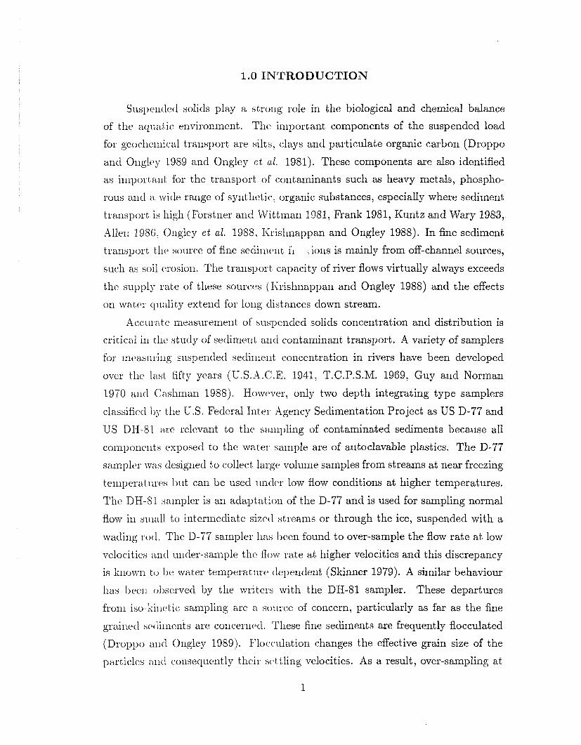
1.0 INTRODUCTION

Susl)c~litlccl solids play a strolig role in the biological and chemical balance

of tllc acl~ln t ic environment . Tllc inlport ant components of the suspended load

for geoclieliiical transport are silts, clays and particulate organic carbon (Droppo

and Oligley 1989 and Ongley e t (11. 1081). These components are also identified

as inlporta~it for the transport of rontaminants such as heavy metals, phospho-

rous alicl a wide range of syntlietic, organic substances, especially where sediment

transport is high (Forstner ancl Wittl~lan 1981, Frank 1981, Kuntz and Wary 1983,

Allen 1986, Origley e t al. 1988, I\;rishnappan and Ongley 1988). In fine sediment

tralislx~rt the source of fine seclinie~lt G ,ions is mainly from off-channel sources,

sucli as soil c.rosion. The transport capacity of river flows virtually always exceeds

the supply rate of these sources (Iirishnappan and Ongley 1988) and the effects

011 water clunlity extend for long distances down stream.

Accl~rate measurement of' susl,eliclecl solids concentration and distribution is

critical ill tlic. study of sediment alitl contaminant transport. A variety of samplers

for ~lleasur,ilig suspended sedi~li~li t concentration in rivers have been developed

over tllc laht fifty years (U.S.A.C.E. 1941, T.C.P.S.M. 1969, Guy and Norman

1970 ant1 Cash~ilan 1988). Howover, only two depth integrating type samplers

clsssifictl1)y tlie U .S. Federal Inter- Agency Sedimentation Project as US D-77 and

US DH-81 ;IS(. relevant to tlic. sn~iil~ling of contaminated sediments because all

coniporic~~its exposed to the water saniple are of autoclavable plastics. The D-77

saml~lcr was designed to collect large. volume samples from streams at near freezing

teniperatures hut can be used untler low flow conditions at higher temperatures.

Tlic DH-81 sanipler is an adaptatioii of the D-77 and is used for sampling normal

flow ill siiinll to intermediate sizecl streams or through the ice, suspended with a

~vacling rotl. The D-77 sampler lias l~een found to over-sample the flow rate at low

velocities tuitl u~ider-sample the flow rate at higher velocities and this discrepancy

is l;~iow~i t o I )e water temperat 1u.c. clependent (Skinner 1979). A similar behaviour

llas 11ec.li ol)sesved by the writers with the DH-81 sampler. These departures

fro111 iso-ki~ic.tic sampling are a so~u.ce of concern, particularly as far as the fine

grained sc~cliincnts are concernc~d. Tliese fine sediments are frequently flocculated

(DroP1)o ant1 Oligley 1989). Flot-culation changes the effective grain size of the

particles t~iitl co~lseclucntly t1it.i~ sc>t,t!ing velocities. As a result, over-sampling at

low velocities may actually mis-represent the true sediment size and structure in

the water column. Over or under-sampling may also mis-represent any short term

temporal variations in sediment and water chemistry which may exist during the

vertical transit time of the sampler. This size and/or chemical mis-representation

can have significant implications from a water and sediment quality perspective.

Therefore, it is important that a sampler be iso-kinetic at all velocity ranges.

Sediment loads and properties as well as water chemistry of small rivers in

Ontario are an important component of the research program at the National

Water Research Institute in which the DH-81 suspended sediment sampler is used

extensively. In an effort to improve the performance of this type of sampler,

preliminary tests were conducted in the towing tank of the Institute's hydraulics

laboratory to investigate the possibility of obtaining iso-kinetic calibrations. The

results of this study are presented in this report.

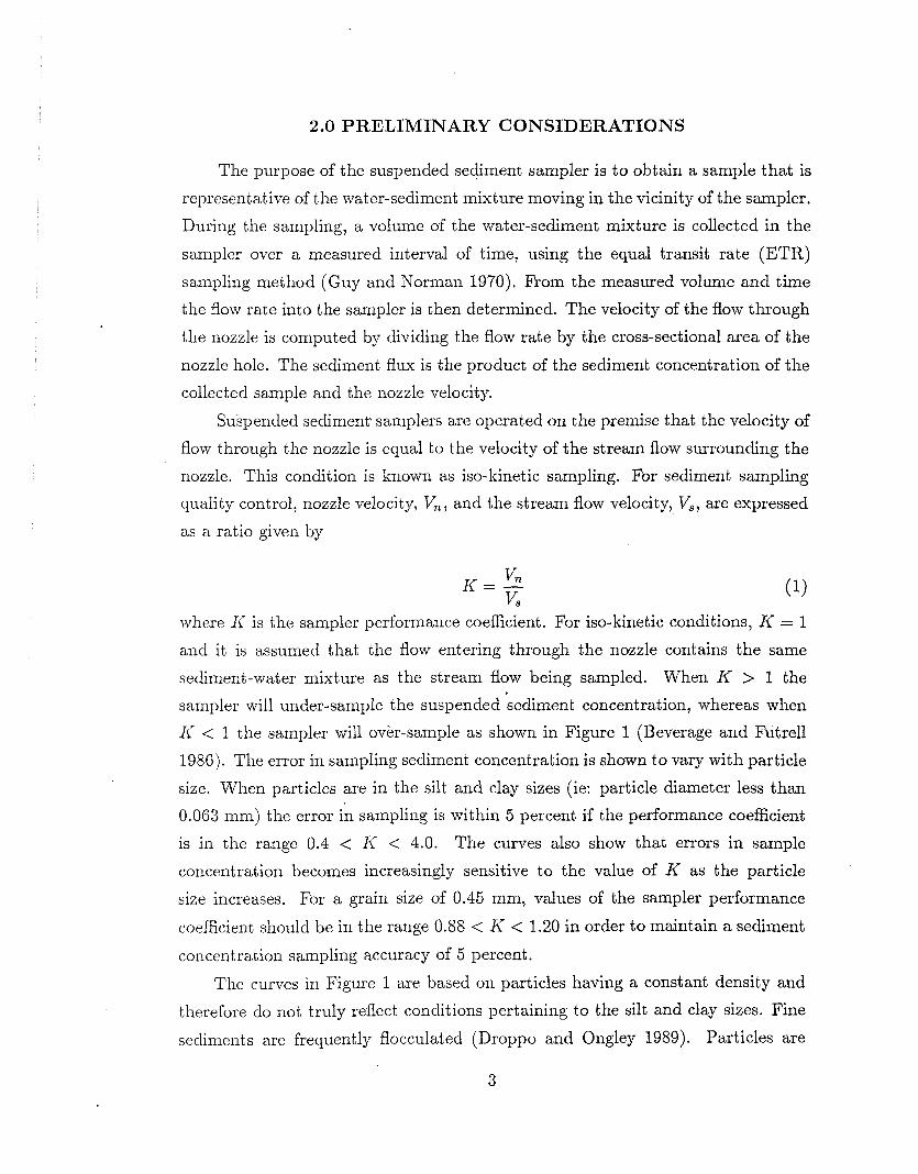
2.0 PRELIMINARY CONSIDERATIONS

The purpose of the suspended sediment sampler is to obtain a sample that is

represent at ive of the water-sediment mixture moving in the vicinity of the sampler.

During the sampling, a volume of the water-sediment mixture is collected in the

sampler over a measured interval of time, using the equal transit rate (ETR)

sampling method (Guy and Norman 1970). From the measured volume and time

the flow rate into the sampler is then determined. The velocity of the flow through

the nozzle is computed by dividing the flow rate by the cross-sectional area of the

nozzle hole. The sediment flux is the product of the sediment concentration of the

collected sample and the nozzle velocity.

Suspended sediment. samplers are operated on the premise that the velocity of

flow through the nozzle is equal to the velocity of the stream flow surrounding the

nozzle. This condition is known as iso-kinetic sampling. For sediment sampling

quality control, nozzle velocity, V,, and the stream flow velocity, V,, are expressed

as a ratio given by

where K is the sampler performance coefficient. For iso-kinetic conditions, I{ = 1

and it is assumed that the flow entering through the nozzle contains the same

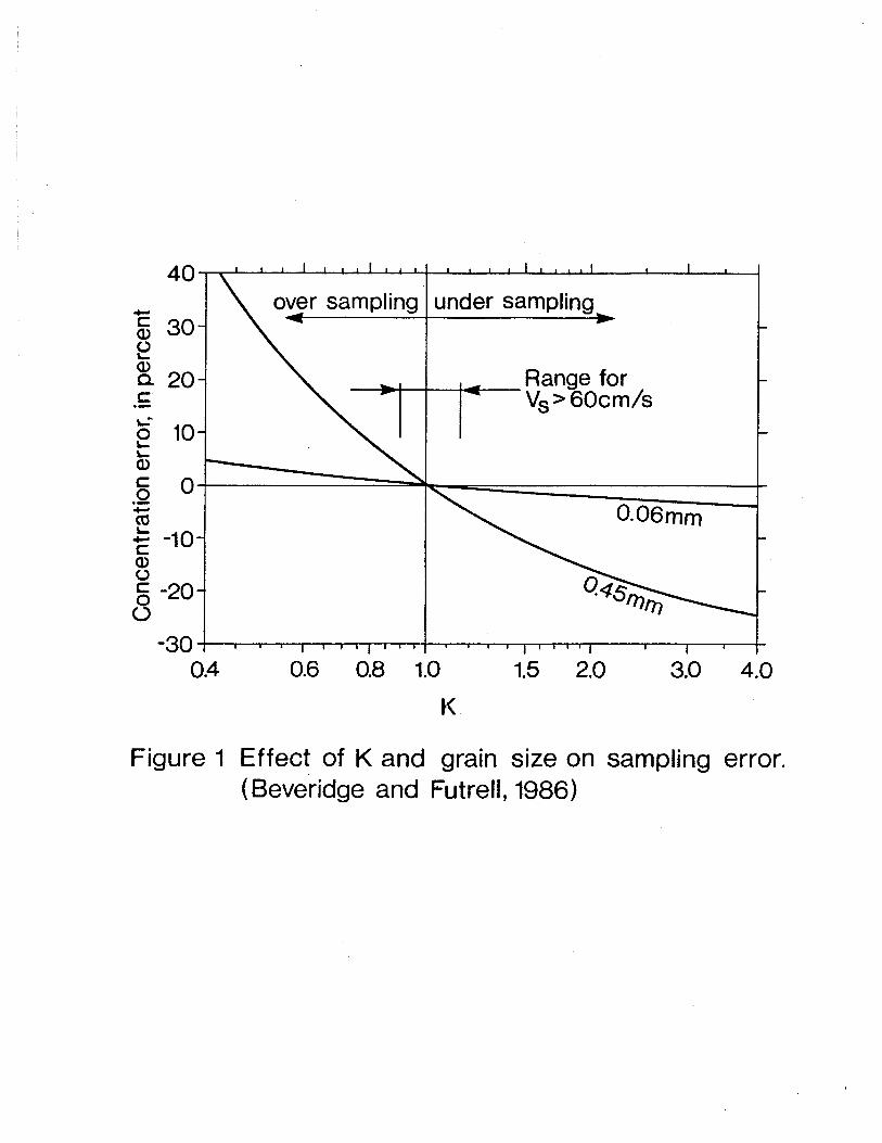
sediment-water mixture as the stream flow being sampled. When I< > 1 the

sampler will under-sample the suspended sediment concentration, whereas when

I< < 1 the sampler will over-sample as shown in Figure 1 (Beverage and Futrell

1986). The error in sampling sediment concentration is shown to vary with particle

size. When particles are in the silt and clay sizes (ie: particle diameter less than

0.063 mm) the error in sampling is within 5 percent if the performance coefficient

is in the range 0.4 < I< < 4.0. The curves also show that errors in sample

concentration becomes increasingly sensitive to the value of K as the particle

size increases. For a grain size of 0.45 mm, values of the sampler performance

coefficient should be in the range 0.88 < II < 1.20 in order to maintain a sediment

concentration sampling accuracy of 5 percent.

The curves in Figure 1 are based on particles having a constant density and

therefore do not truly reflect conditions pertaining to the silt and clay sizes. Fine

sediments are frequently flocculated (Droppo and Ongley 1989). Particles are

bonded together to produce single units called flocs. These flocs behave as single

particles having an effective diameter many times larger than the original, com-

ponent particles but having a lower density depending on their compactness. The

tendency toward larger sampling errors as a result of increased particle size is off-

set by the lower density of the flocs. However, for the silt and clay sizes, sampling

errors greater than those indicated in Figure 1, can be expected.

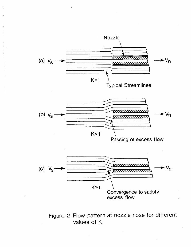
The reasons for these effects at different values of I< are as follows: If K =

1, the stream flow will pass straight into the nozzle while any stream lines on

either side of the nozzle intake will be deflected as shown in Figure 2(a). For

this condition the trajectories of the sediment articles are parallel to the stream

lines of the flow entering the nozzle. As a result the sampler collects the correct

proportion of water and sediment particles. When K < 1, the velocity in the

nozzle will be slower than the stream flow velocity and, as a result, an area of

stagnation will develop at the head of the nozzle as shown in Figure 2(b). In

this case the stream lines of the approaching flow will be deflected ahead of the

nozzle entrance. However, the sediment particles, because of their inertia, will

tend to continue on their original path toward the nozzle entrance. As a result,

for a given sampling time, the sampler will under-sample the water volume but

collect a larger proportion of sediment particles, resulting in over-sampling of the

sediment concentration. Finally, when K > 1, the velocity in the nozzle will be

greater than that of the approaching flow and stream lines in the vicinity of the

nozzle will converge toward the nozzle intake as shown in Figure 2(c). Once again

the sediment particles will resist the sudden change in direction and the increase

in water flow through the nozzle will not be accompanied by a corresponding

increase in sediment particles. As a result, the sampler will under sample the

sediment concent rat ion.

In general, particle sizes in suspension are largely a function of flow velocity

and level of turbulence, and therefore, a wide range of particle sizes can be obtained

in a given sample. It is important to ensure that the samplers are capable of

sampling iso-ltinetically.

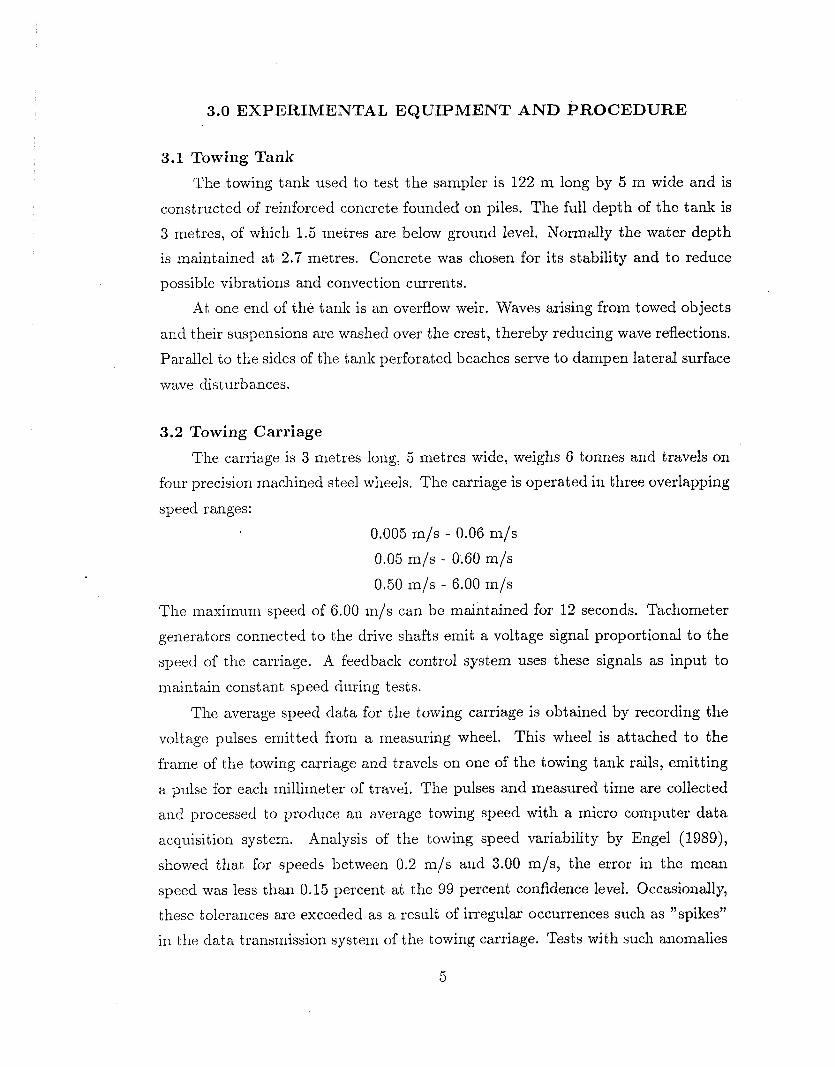
3.0 EXPERIMENTAL EQUIPMENT A N D PROCEDURE

3.1 Towing Tank

The towing tanlc used to test the sampler is 122 m long by 5 m wide and is

constructed of reinforced concrete founded on piles. The full depth of the tank is

3 metres, of which 1.5 metres are below ground level. Normally the water depth

is maintained at 2.7 metres. Concrete was chosen for its stability and to reduce

possible vibrations and convection currents.

At one end of the tank is an overflow weir. Waves arising from towed objects

and their suspensions are washed over the crest, thereby reducing wave reflections.

Parallel to the sides of the tanlc perforated beaches serve to dampen lateral surface

wave disturbances.

3.2 Towing Carriage

The carriage is 3 metres long, 5 metres wide, weighs 6 tonnes and travels on

four precision machined steel wheels. The carriage is operated in three overlapping

speed ranges:

0.005 m/s - 0.06 m/s

0.05 m/s - 0.60 m/s

0.50 m/s - 6.00 m/s

The maximum speed of 6.00 m/s can be maintained for 12 seconds. Tachometer

generators connected to the drive shafts emit a voltage signal proportional to the

speed of the carriage. A feedback control system uses these signals as input to

maint a h const ant speed during tests.

The average speed data for the towing carriage is obtained by recording the

voltage pulses emitted from a measuring wheel. This wheel is attached to the

frame of the towing carriage and travels on one of the towing tank rails, emitting

a pulse for each millimeter of travel. The pulses and measured time are collected

and processed to produce an average towing speed with a micro computer data

acquisition system. Analysis of the towing speed variability by Engel (1989),

showed that for speeds between 0.2 m/s and 3.00 m/s, the error in the mean

speed was less than 0.15 percent at the 99 percent confidence level. Occasionally,

these tolerances are exceeded as a result of irregular occurrences such as "spikes"

in the data transmission system of the towing carriage. Tests with such anomalies

are recognized by the computer and are automatically abandoned.

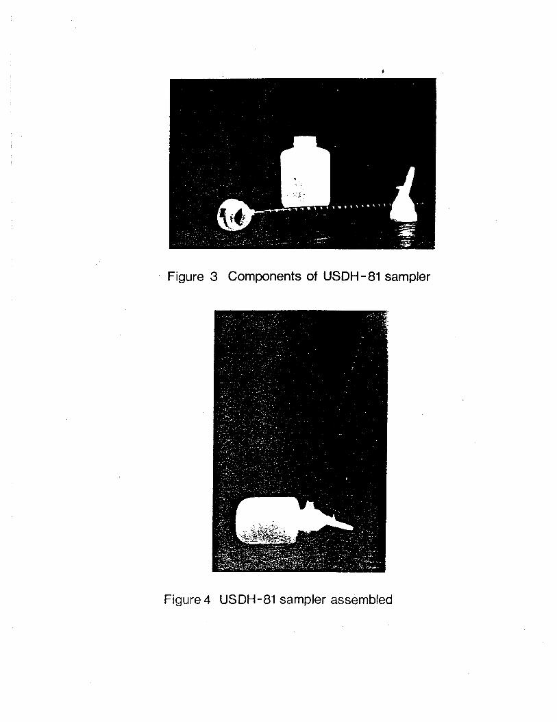
3.3 The DH-81 Sampler and Appurtenances

The sampler consists of a DH-81 adapter, a US D-77 cap, a standard 7.94 mm

inside diameter nozzle, a plastic "mason-jar" threaded bottle with 3 litre capacity

and a wading rod. The components of the sampler are given in Figure 3 and the

assembled sampler is given in Figure 4.

The US DH-81 sampler is designed to sample low velocity rivers by wading

or by sampling through the ice cover (Cashman 1988). The sampler allows for

large sample volu~nes (2700 ml), providing the large samples required for sedimen-

tological analysis. When used in conjunction with a plastic bottle the sampler is

useful for chemical and biological studies as all the components which contact the

water sample are composed of autoclavable plastic. When the sampler is lowered

into the flow, air is expelled through a 3.0 mm diameter air vent at the top of the

sampler cap. A small "horn" protruding from the sampler cap just ahead of the

air vent presents a "bluff" body to the flow resulting in a small negative pressure

pocket immediately behind it. This creates a "suction" effect which effectively re-

duces the energy drop through the air vent. Finally, the air vent outlet is located

about 2 cm above the centre-line of the nozzle flow passage. This creates a small

positive, net hydro-static pressure which is constant regardless of the depth of the

sampler.

3.4 Effect of Flow Depth

The D-77 and the DH-81 sampler are open to the outside environment during

the depth integrated sampling process. As a result, the air volume inside the

samplers is subject to the effect of pressure changes as the sampler is lowered

and raised through the flow. Initially, at the surface, the internal cavity of the

sampIer is at atmospheric pressure because the sampler is open to the air through

the nozzle and the air vent. As the sampler is submerged and travels toward

the stream bed, the pressure inside the sampler increases in proportion to the

flow depth. The increase in static pressure compresses the volume of air in the

sampler and this causes an inflow of water in excess of that expected due to the

net head (H, + velocity head; where H , is the static head at the nozzle equal to

the difference in elevation of the centre-line of the nozzle and the air vent) alone.

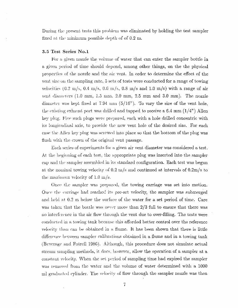
During t,lic l)sese~it tests tliis prol~lc~m was eliminated by holding the test sampler

fixed a t tllo ilii~limurn possible clcl)tll of of 0.2 m.

3.5 Test Series No.1

For 21 givcri nozzle the volu~iic~ of water that can enter the sampler bottle in

a given l)(>siod of time should clel>encl, anlong other things, on the the physical

propestics of the riozzle ancl the air vent. In order to determine the effect of the

vent size. 011 tlie sampling rate, 5 sets of tests were conducted for a range of towing

velocities (0.2 ~ n / s , 0.4 m/s, O.G ~i i /s , 0.8 m/s and 1.0 m/s) with a range of air

vent tliairlc.tt.rs (1.0 mm, 1.5 mni, 2.0 mm, 2.5 mrn and 3.0 mm). The nozzle

dia~iietcs was kept fixed at 7.94 111111 (5/16"). To vary the size of the vent hole,

the existi~ig esliaust port was clsill(~c1 and tapped to receive a 6.4 mm (114") Allen

key plug. Fivc such plugs were lxcl~ared, each with a hole drilled concentric with

its longituclilial axis, to provide tlie new vent hole of the desired size. For each

case the -4ll(~n liey plug was scscwc~l into place so that the bottom of the plug was

flush witli tlic. crown of the original vent passage.

Eacli series of experinlerits for a given air vent diameter was considered a test.

At the bcgiiining of each test, t l i ~ appropriate plug was inserted into the sampler

cap a~icl tlir sampler assemhlccl in it,s standard configuration. Each test was begun

at tlie ~ioliii~ial towing velocity of 0.2 11i/s and continued at intervals of 0.2m/s to

the ul:~si~iiulil velocity of 1.0 ~i l /s .

0xicc. tlie sampler was psepascd, the towing carriage was set into motion.

Once. t lit> c.:issiage hacl reacllecl its pre-se t velocity, the sampler was submerged

ancl lielcl a t 0.2 ~n below the swface of the water for a set period of time. Care

was taliell tAat the bottle was nc1 c.1- more than 213 full to ensure that there was

no intcrf(~rc~~ice in the air flow through the vent due to over-filling. The tests were

conductccl ill a towing tank I>ecausc. this afforded better control over the reference

velocity tlla~i can be obtaillecl in a flume. It has been shown that there is little

diff'esc~licc~ I)c.t~vec~~i sa~llpler calil~ratious obtained in a flume and in a towing tank

(Be~resagch a~icl F~~ t re l l 19%). .4lt,llough, this procedure does not simulate actual

stseani saiiiljling methods, it does, llowever, allow the operation of a sampler at a

consta~lt vc>locity. When the set ~)oriod of sampling time had expired the sampler

was scnio~ic~l from the water a~icl tlie volume of water determined with a 1000

ml grn t l~~atc~l cyli~icler. The velocity of flow through the sampler nozzle was then

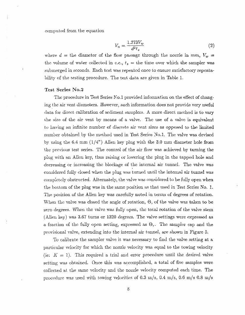
computed from the equation

where d = the diameter of the flow passage through the nozzle in mm, V, =

the volume of water collected in c.c., t , = the time over which the sampler was

submerged in seconds. Each test was repeated once to ensure satisfactory repeata-

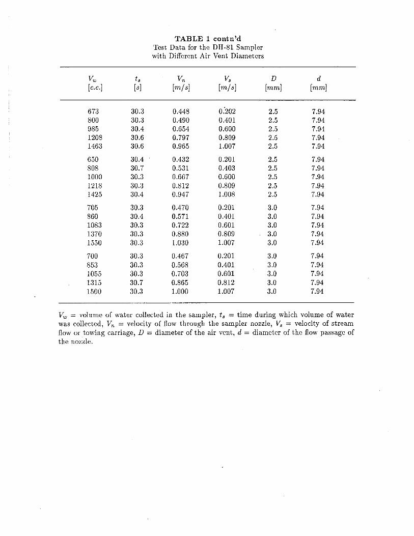
bility of the testing procedure. The test data are given in Table 1.

Test Series No.2

The procedure in Test Series No.1 provided information on the effect of chang-

ing the air vent diameters. However, such information does not provide very useful

data for direct calibration of sediment samplers. A more direct method is t'o vary

the size of the air vent by means of a valve. The use of a valve is equivalent

to having an infinite number of discrete air vent sizes as opposed to the limited

number obtained by the method used in Test Series No.1. The valve was devised

by using the 6.4 mm (1/4") Allen key plug with the 3.0 mm diameter hole from

the previous test series. The control of the air flow was achieved by turning the

plug with an Allen key, thus raising or lowering the plug in the tapped hole and

decreasing or increasing the blockage of the internal air tunnel. The valve was

considered fully closed when the plug was turned until the internal air tunnel was

completely obstructed. Alternately, the valve was considered to be fully open when

the bottom of the plug was in the same position as that used in Test Series No. 1.

The position of the Allen key was carefully noted in terms of degrees of rotation.

When the valve was closed the angle of rotation, 0, of the valve was taken to be

zero degrees. When the valve was fully open, the total rotation of the valve stem

(Allen key) was 3.67 turns or 1320 degrees. The valve settings were expressed as

a fraction of the fully open setting, expressed as 0,. The sampler cap and the

provisional valve, extending into the internal air tunnel, are shown in Figure 5.

To calibrate the sampler valve it was necessary to find the valve setting at a

particular velocity for which the nozzle velocity was equal to the towing velocity

(ie: I< = 1). This required a trial and error procedure until the desired valve

setting was obtained. Once this was accomplished, a total of five samples were

collected at the same velocity and the nozzle velocity computed each time. The

procedure was used with towing velocities of 0.3 m/s, 0.4 m/s, 0.6 m/s 0.8 m/s

and 1.0 m/s. The nozzle velocities were determined in the same way as in Test

Series No.1. The data are given in Table 2.

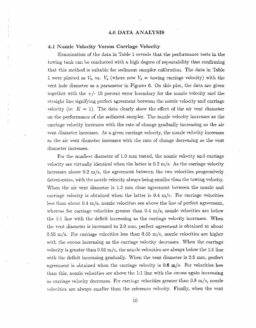
4.0 DATA ANALYSIS

4.1 Nozzle Velocity Versus Carriage Velocity

Examination of the data in Table 1 reveals that the performance tests in the

towing tank can be conducted with a high degree of repeatability thus confirming

that this method is suitable for sediment sampler calibration. The data in Table

1 were plotted as V, vs. Vs (where now Vs = towing carriage velocity) with the

vent hole diameter as a parameter in Figures 6. On this plot, the data are given

together with the +/- 15 percent error boundary for the nozzle velocity and the

straight line signifying perfect agreement between the nozzle velocity and carriage

velocity (ie: I{ = 1). The data clearly show the effect of the air vent diameter

on the performance of the sediment sampler. The nozzle velocity increases as the

carriage velocity increases with the rate of change gradually increasing as the air

vent diameter increases. At a given carriage velocity, the nozzle velocity increases

as the air vent diameter increases with the rate of change decreasing as the vent

diameter increases.

For the smallest diameter of 1.0 mm tested, the nozzle velocity and carriage

velocity are virtually identical when the latter is 0.2 m/s. As the carriage velocity

increases above 0.2 m/s, the agreement between the two velocities progressively

deteriorates, with the nozzle velocity always being smaller than the towing velocity.

When the air vent diameter is 1.5 mm close agreement between the nozzle and

carriage velocity is obtained when the latter is 0.4 m/s. For carriage velocities

less than about 0.4 m/s, nozzle velocities are above the line of perfect agreement,

whereas for carriage velocities greater than 0.4 m/s, nozzle velocities are below

the 1:l line with the deficit increasing as the carriage velocity increases. When

the vent diameter is increased to 2.0 mm, perfect agreement is obtained at about

0.55 m/s. For carriage velocities less than 0.55 m/s, nozzle velocities are higher

with the excess increasing as the carriage velocity decreases. When the carriage

velocity is greater than 0.55 m/s, the nozzle velocities are always below the 1:l line

with the deficit increasing gradually. When the vent diameter is 2.5 mm, perfect

agreement is obtained when the carriage velocity is 0.8 m/s. For velocities less

than this, nozzle velocities are above the 1:l line with the excess again increasing

as carriage velocity decreases. For carsia.ge velocities greater than 0.8 m/s, nozzle

velocities are always smaller than the reference velocity. Finally, when the vent

diameter is 3.0 mm, perfect agreement is obtained when the carriage velocity is

1.0 m/s. For carriage velocities less than this, nozzle velocities are always above

the line of perfect agreement with the excess increasing as the reference velocity

decreases. For carriage velocities greater than 1.0 m/s, as observed for the previous

vent diameters, the opposite is true.

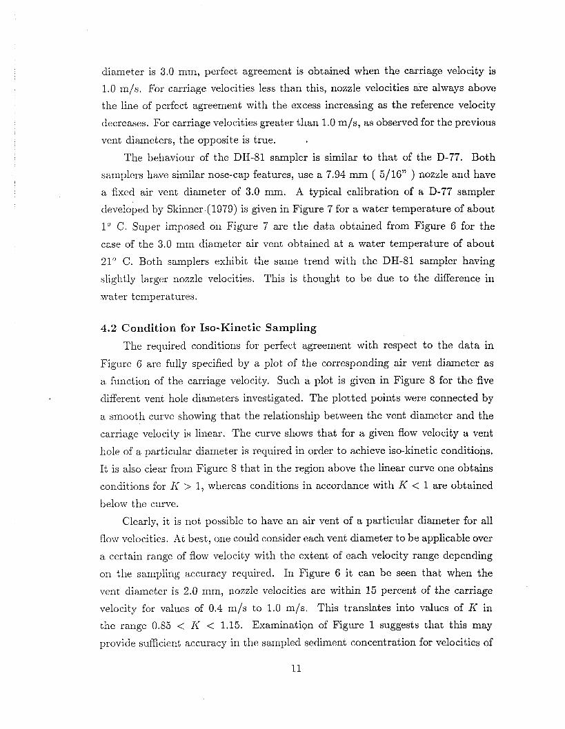
The behaviour of the DH-81 sampler is similar to that of the D-77. Both

samplers have similar nose-cap features, use a 7.94 mm ( 5/16" ) nozzle and have

a fixed air vent diameter of 3.0 mm. A typical calibration of a D-77 sampler

developed by Skinner.(1979) is given in Figure 7 for a water temperature of about

lo C. Super imposed on Figure 7 are the data obtained from Figure 6 for the

case of the 3.0 mm diameter air vent obtained at a water temperature of about

21" C. Both samplers exhibit the same trend with the DH-81 sampler having

slightly larger nozzle velocities. This is thought to be due to the difference in

water temperatures.

4.2 Coiiditioii for Iso-Kinetic Sanlpling

The required conditions for perfect agreement with respect to the data in

Figure 6 are fully specified by a plot of the corresponding air vent diameter as

a function of the carriage velocity. Such a plot is given in Figure 8 for the five

different vent hole diameters investigated. The plotted points were connected by

a smooth curve showing that the relationship between the vent diameter and the

carriage velocity is linear. The curve shows that for a given flow velocity a vent

hole of a particular diameter is required in order to achieve iso-kinetic conditions.

It is also clear from Figure 8 that in the region above the linear curve one obtains

conditions for I< > 1, whereas conditions in accordance with K < 1 are obtained

below the curve.

Clearly, it is not possible to have an air vent of a particular diameter for all

flow velocities. At best, one could consider each vent diameter to be applicable over

a certain range of flow velocity with the extent of each velocity range depending

on the sampling accuracy required. In Figure 6 it can be seen that when the

vent diameter is 2.0 mm, nozzle velocities are within 15 percent of the carriage

velocity for values of 0.4 m/s to 1.0 m/s. This translates into values of II in

the range 0.85 < II < 1.15. Examination of Figure 1 suggests that this may

provide sufficient accuracy in the sampled sediment concentration for velocities of

0.4 m/s to 1.0 m/s. When the carriage velocity is 0.2 m/s, the nozzle velocity

obtained is about 0.41 m/s, representing an error of 105 percent, which translates

into I< = 2.05. According to Figure 1, such a value of I< is acceptable for clay

to silt size particles, however, as flow velocities approach values between 0.2 m/s

to 0.4 m/s, particle sizes can be expected to be larger and values of I< in the

range 0.85 < I< < 1.15 would be more desirable. Further examination of Figure 6

reveals that selection of another air vent diameter would not be practical, because

at carriage velocities less than 0.4 m/s, for each chosen value of air vent diameter,

nozzle velocities would be within 15 percent error envelopes over a very narrow

range of the reference velocities. Some improvement can be achieved by using an

air vent diameter of about 1.50 mm at flow velocities of 0.4 m/s and less, This

would ensure that the nozzle velocities would be inside the 15 percent error bands

for flow velocities between 0.3 m/s and 0.4 m/s and reduces the value of I< from

2.05 when the vent diameter is 2.0 mm to 1.63 when the vent diameter is 1.5

mm. At the very low flows, there is also a concern about flocculation, resulting in

effective particle diameters larger than the, individual component particles. These

larger particles further increase the need for iso-kinetic sampling for flows near

velocities of 0.2 m/s. The data in Figure 6 suggest that in this case an air vent

diameter of 1.0 mm should be used. Although, using different air vent diameters

provides some improvement, it is obvious that the use of discrete air vent sizes is

not a fully satisfactory solution.

4.3 Continuous Air Vent Control

The data in Table 2 were organized so that the rotation of the air valve at

any given position was expressed as a fraction of the fully open position. The

data were then plotted as O, versus the carriage velocity in Figure 9. A smooth

curve was fitted through the plotted points to facilitate the analysis. The curve

represents the flow control curve for the DH-81 sampler, showing a gradual increase

in O , as the carriage velocity increases, with the rate of change in O, increasing

or, conversely, the sensitivity of the valve decreasing. When the carriage velocity

is 1.0 m/s, the curve indicates that the upper limit of the air valve has been

virtually reached. During the tests it was not possible to obtain consistent results

at a carriage velocity of 0.2 m/s. Howcver, tests at a velocity of 0.3 m/s were

successful. Therefore, for the present valve configuration it was concluded that

the lowest operating limit is about 0.25 m/s. It is most probable, that at such

low velocities, the total pressure head driving the flow into the sampler nozzle is

not great enough to overcome the energy losses of the air flow passing through the

valve. Further development worlc is required to overcome this problem at low flow

velocities.

Although the air valve has been crudely contrived, the data in Figure 9 indi-

cate that a consistent relationship between the valve opening and the flow velocity

is possible. Therefore, such a valve is a viable and practical alternative to the

discrete air vent sizes discussed in the previous section.

The mean nozzle velocities obtained at each valve setting for a particular

carriage velocity are plotted as Figure 10. Tests at each carriage velocity were

conducted five times. All points fall on the line of perfect agreement, signifying

a value of Ii' = 1. These results further substantiate that the DH-81 sediment

sampler performance can be controlled with a high degree of repeatability by

using an air vent valve. Clearly, for this type of sampler, the control of the flow

into the sampler is governed by the valve and not by the hydraulic characteristics

of the nozzle.

A curve of O r vs. V,, as given in Figure 9, represents the calibration curve for

a particular sampler. Further tests should be conducted to see if a single generic

curve can be used for all DH-81 samplers.

5.0 GENERAL CALIBRATION EQUATION

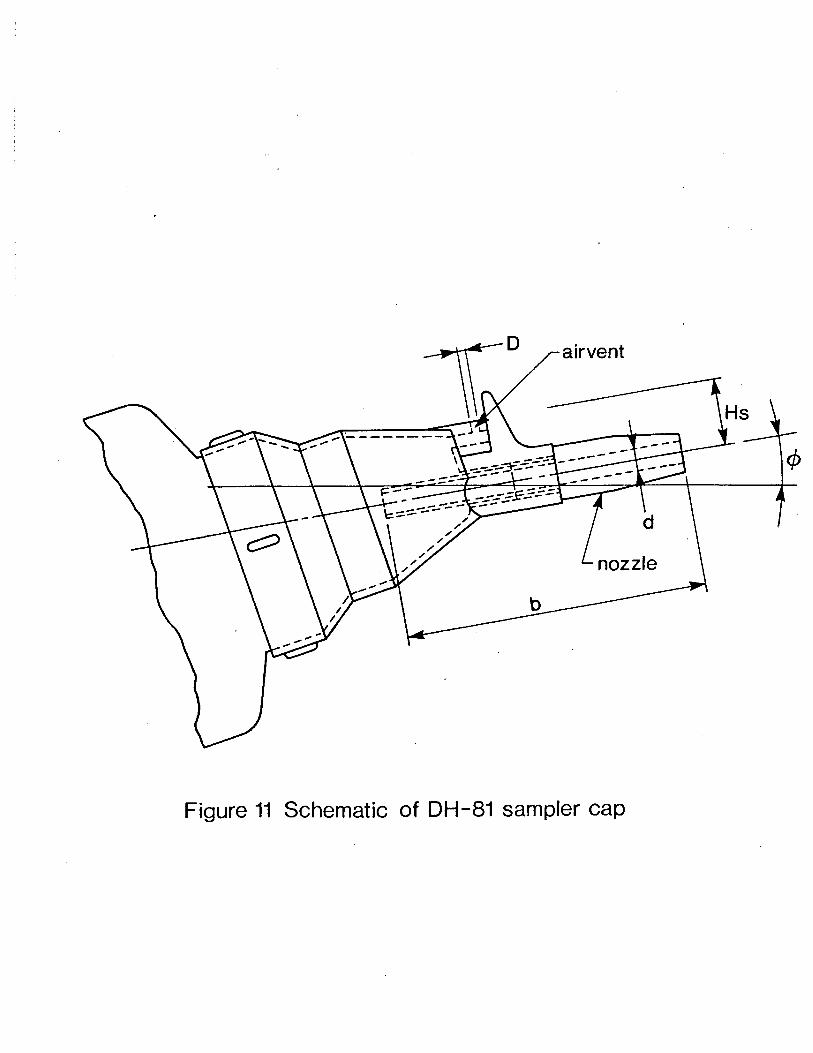
5.1 Diilleiisioilal Ailalysis

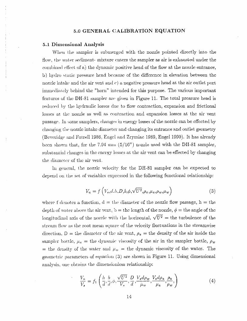
VTllen tlle sampler is subnlergecl with the nozzle pointed directly into the

flow, tlic water sediment- mixture (.liters the sampler as air is exhausted under the

conllined cEcct of a) the dynanlic positive head of the flow at the nozzle entrance,

b) hydro static pressure head because of the difference in elevation between the

nozzle i~itakc arid the air vent and c ) a negative pressure head at the air outlet port

imnlediatclly behind the "horn" i~ltc~icled for this purpose. The various important

features of the DH-81 sampler arc given in Figure 11. The total pressure head is

reclucecl 1 ) ~ . the hydraulic losses clue to flow contraction, expansion and frictional

losses at tllr. nozzle as well as co~ltraction and expansion losses at the air vent

passage. 111 some samplers, changes in energy losses of the nozzle can be effected by

changing t l l ~ nozzle intake cliameter and changing its entrance and outlet geometry

(Bevcriclgc. ancl Futrell 1986, Engel ant1 Zrymiac 1989, Engel 1990). It has already

been s l lo~~ l l tliat, for the 7.94 111111 (5116") nozzle used with the DH-81 sampler,

substa~itial c-llanges in the energy losses at the air vent can be effected by changing

the clia111r.tc~r of the air vent.

111 gc~licral, the nozzle velocity for the DH-81 sampler can be expected to

clepencl 011 the set of variables esl>ressed in the following functional relationship:

where f tl(~iotcs a function, d = tllc diameter of the nozzle flow passage, h = the

clep t 11 of wa t cr above the air vent, b = the length of the nozzle, q5 = the angle of the

longitutli~lill axis of the nozzle mitli the horizontal, 0 = the turbulence of the

strean1 flow as the root mean scluarc. of the velocity fluctuations in the streamwise

clirectio~l, D = the diameter of thc air vent, pa = the density of the air inside the

sampler l )o t tle, p, = the dynamic viscosity of the air in the sampler bottle, p,

= the clcnsity of the water ancl p,,, = the dynamic viscosity of the water. The

geonlc tric l)arameters of ecjuation ( 3 ) are shown in Figure 11. Using dimensional

analysis, olicl obtains the clime~isio~lless relationship:

where f l tlcnotes a dimensioriless function for a particular sampler. Beverage

and Futrc.11 (1986) have sllown that results from tests in towing tanks are not

significa~itly different from results of tests conducted in turbulent flows in flumes. 0 Therefore, thc variable 7 in equation (4) is not very important and can be

omitted fro111 further considerations. The depth of submergence of the sampler

was 1wpt a t 0.2 m and therefore tlie effect of 4 will be negligible and may also

be elilililiatecl from equation (4). Examination of data by Engel and Zrymiac

(1989) a~icl Engel (1990) indicate that the discharge coefficient of nozzles is only

nlilclly del,(:~iclent on the Rey~~olcls number UE!E and over the range of operating P w

temperatures the ratio fi does nut vary significantly. As a result, these last two

vziables ~iiiy also be omitted fro111 equation (4). Combining equations (1) and

(4) one obtains

wherc f;! (l(:~iotes another dimensio~lless function. In general, equation (5) shows

the vasious clirlle~lsionless variables that can affect the value of K. In this study,

tests were conducted with a sempli-r liaving fixed values of $ and q5 = 0. Therefore

for prc~selit pusposes equation (5) can be reduced to

wherc j:] clcliotes another di~llensionless function. For the case of valve control

the effective vent opening is governed by the adjustment of the air vent valve.

Therefore, Ly introducing the dir~~er~sionless valve setting O,, equation (6) may

now be ex1,ressecl in an alternate form as

where fSl clcnotes another dimensio~lless function. Finally, the calibration curve

lliust exist for the special case of I< = 1 and for this case, one may now write the

dinlensio~llcss calibration curve as

whew .f5 <Icnotes another dimensionless function.

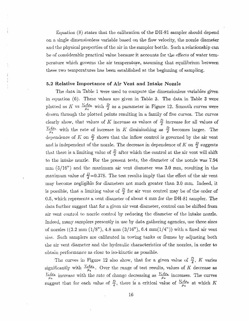
Equation (8) states that the calibration of the DH-81 sampler should depend

on a single dimensionless variable based on the flow velocity, the nozzle diameter

and the physical properties of the air in the sampler bottle. Such a relationship can

be of considerable practical value because it accounts for the effects of water tem-

perature which governs the air temperature, assuming that equilibrium between

these two temperatures has been established at the beginning of sampling.

5.2 Relative Iinportailce of Air Vent and Intake Nozzle

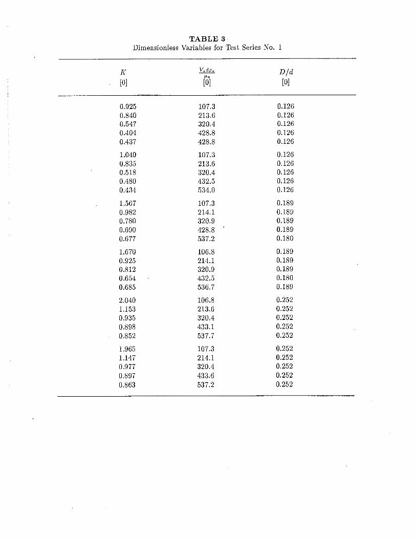
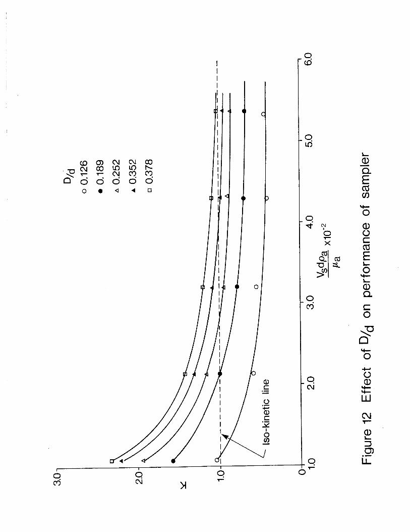
The data in Table 1 were used to compute the dimensionless variables given

in equation (6). These values are given in Table 3. The data in Table 3 were

plotted as I< vs 7 Vs d p a with $ as a parameter in Figure 12. Smooth curves were

drawn through the plotted points resulting in a family of five curves. The curves

clearly show, that values of K increase as values of 9 increase for all values of

""Q with the rate of increase in I< dimininshing as 9 becomes larger. The l j a

dependence of I< on $ shows that the inflow control is governed by the air vent

and is independent of the nozzle. The decrease in dependence of IC on 9 suggests

that there is a limiting value of $ after which the control at the air vent will shift

to the intake nozzle. For the present tests, the diameter of the nozzle was 7.94

mm (5116") and the maximum air vent diameter was 3.0 mm, resulting in the

maximum value of $=0.378. The test results imply that the effect of the air vent

may become negligible for diameters not much greater than 3.0 mm. Indeed, it

is possible, that a limiting value of $ for air vent control may be of the order of

0.5, which represents a vent diameter of about 4 mm for the DH-81 sampler. The

data further suggest that for a given air vent diameter, control can be shifted from

air vent control to nozzle control by reducing the diameter of the intake nozzle.

Indeed, many samplers presently in use by data gathering agencies, use three sizes

of nozzles ((3.2 mm (1/8"), 4.8 mm (3/16"), 6.4 mm(1/4")) with a fixed air vent

size. Such samplers are calibrated in towing tanks or flumes by adjusting both

the air vent diameter and the hydraulic characteristics of the nozzles, in order to

obtain performance as close to iso-kinetic as possible.

The curves in Figure 12 also show, that for a given value of $, K varies

significantly with *. Over the range of test results, values of I< decrease as

' p a increase with the rate of change decreasing as increases. The curves Pa

suggest that for each value of 8, there is a critical value of at which K

l~eco~iies i~iclepe~lde~lt of Jkh Pa

. When 5= 0.176, the critical value of is P a

about GOO. Tlle critical value of increases slightly as 9 increases. fLn

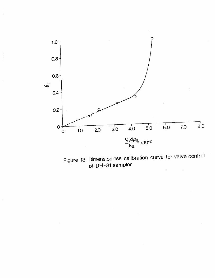
5.3 Di~~leiisionless Calibratioil Curve

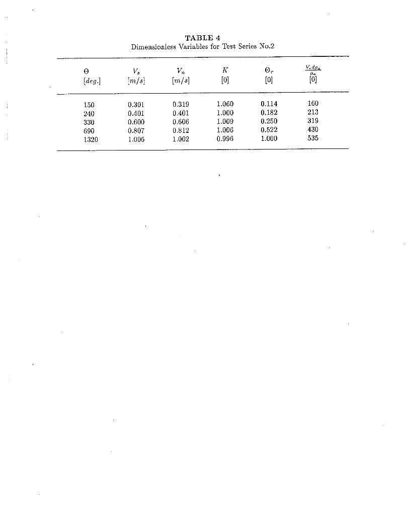
Tlie cln ta in Table 2 were used to compute the dimensionless variables given in

ecpt~tio~is (8) . These values are givcn in Table 4. The data in Table 4 were plotted

in Figure. 13 as O r vs. - . Tlle form of the curve is similar to that of Figure 8. Pa

Values of (-1, increase al~nost linearly as increases. When the latter reaches V d p a value of al,out 500, E),. begins to increase sharply with further increases in y,

inclic;~ti~ig tliat there is a limiting value at which ELPA becomes independent of P a

O,.. At this critical point, control of the flow into the sampler would change from

the air \rc31it to the intalte nozzle.

Tile c-~~rve in Figure 13 has tlic advantage of including the fluid properties as

well as t,lic size of the nozzle. The. c5urve indicates that for a given flow velocity, if

the intalw tliarlleter of the ~~ozzle is seduced, then is reduced and 0, must be P a

reducc~tl ill acacordance with the estalIlished calibration. In other words, a reduction

in thc. size of tlle nozzle means a rccluction in the rate of change of water volume

inside tlic. salnpler and the valve opening must be reduced in accordance with the

lower flow rate of escaping air, tliereby ensuring that iso-kinetic conditions are

maintai~ic~tl. It is also clear fro111 tlie dinlensionless calibration curve that water

teml~eraturc. ~llust be considered wllen the sampler is used to allow for changes in

fluicl vise-osit y.

Tlle cli~lle~lsio~lless calibratiorl curve in Figure 13 accounts for the fluid temper-

ature. This call be demonst rated, with available data, by plotting the relationship

give11 11y c.cluation (6) sing the, test data of the DH-81 sampler for the special

case of tlic. 3.0 mrri diameter air vc~it. The appropriate data are plotted in Figure

14 as Ii' vs. u. The data were obtained in water at a temperature of 20°C. f ' a

Superi~lil~osecl on the plot are tlic. data obtained from Skinner (1979) obtained

with ;I D-77 sampler having tlie salne diameter nozzle and sampler cap geometry

at i~ watc3r tc~ilperature of about 1°C'. The plot shows that K declines as Pa

increases with tlle rate of clecreasc. diminishing. It is also quite evident that both

sets of c1a.ta collapse to form a, single curve. This strongly suggests that a single

cli~nensionlcss curve such as give11 in Figure 13 and 14 can be used to account

for tlw clltuiges in average air ~>rol,erties for all water temperatures likely to be

encountered during field operations. Separate curves for each temperature are no

longer necessary. However, the general validity of the dimensionless calibration

curve needs to be confirmed with additional tests. Tests should be conducted at

several different water temperatures with at least three different nozzle sizes but

having the same external geometry.

6.0 CONCLUSIONS

Tests, conducted in a towing tank, to establish a calibration curve for the US

DH-81 suspended sediment sampler have led to the following conclusions:

6.1 The velocity of the flow passing through a sampler nozzle of a given size and

geometry is controlled by the ability of the air to discharge through the air vent.

For a given towing velocity, the rate of discharge could be controlled by changing

the diameter of the air vent. The value of the sampling coefficient I{ increased as

the diameter of the air vent was increased. The rate of change in K with change

in air vent diameter was dependent on the towing velocity.

6.2 For a given air vent diameter the sampling coefficient I{ increased as the

towing velocity increased. The rate of increase in I< with the towing velocity

increased slightly as the diameter of the air vent was increased.

6.3 For each of the air vent diameters used there was one towing velocity at which

the sampler behaved iso-kinetically. At all other velocities values of I< were greater

or smaller than the ideal value of 1.0. Over the range of towing velocities from 0.2

m/s to 1.0 m/s, values of I< varied from about 2.2 at a velocity of 0.2 m/s and

an air vent diarrieter of 3.0 mm to a value 0.43 at a velocity of 1.0 m/s and an air

vent diameter of 1.0 mm. The currently operational DH-81 sampler has a fixed

air vent diameter of 3.0 mm and the values of II for velocities from 0.2 m/s to 1.0

m/s vary from 2.2 to 0.94 respectively.

6.4 Analysis of the data indicates that iso-kinetic sampling can be achieved over

the operational velocity range of the sampler by controlling the air flow through

the air vent with a calibrated valve. The sampler can therefore be calibrated in a

towing tank by determining the required valve setting to obtain a value of K = 1

at each selected towing velocity.

6.5 Examination of the test data and data from the literature obtained for tem-

peratures of 20°C and 1°C indicate that for a given flow velocity, nozzle velocities

increase as the temperature increases. Dimensional analysis has shown that a di-

mensionless curve of I< vs. for a given value of g (V, = towing velocity or

flow velocity, d = the internal diameter of the nozzle, D = the diameter of the

air vent, pa = the density of the air in the sampler and pa = the viscosity of the

air in the sampler) can be used to represent the sampler performance. Each sush

curve specifies the value of I< and therefore the sampler performance at all water

temperatures.

6.6 The validity of the dimensionless curves of I< vs. guarantees the validity

of a single dimensionless calibration curve of the air vent valve given as Or vs.

. Therefore, with suit able modifications, the DH-81 suspended sediment P a

sampler as well as the D-77 sampler can be used to sample virtually iso-kinetically

over their full operating range. Theoretically, the dimensionless calibration curve

should also be valid for different sizes of nozzles as long as the valve controls the

flow into the sampler. Work is required to develop a suitable valve for the air vent

control.

6.7 The results indicate that a critical value of exists at which the control of

flow into the sampler changes from the air vent to the intake nozzle. This suggests

that samplers in use today, other than the D-77 and the DH-81, are controlled

either by the air vent or the intake intake nozzles depending on the size of the $ ratio (D= diameter of the air vent, d= diameter of the intake nozzle). Additional

work is required to clearly establish the f l ~ w control regime.

ACKNOWLEDGEMENT

, The writers are grateful to Dr. B.G. Krishnappan and Dr. M.G. Skafel for

their thorough review of the manuscript and their many constructive comments

and discussions. Assistance during the tests was provided by Clarence Bil, David

Blais, Barbara Near and Stephen To. The photographs in Figures 3 and 4 were

taken by Doug Doede. The writers appreciate their dedication to this project.

REFERENCES

Allaii, R.J. 1986. The role of particulate matter in the fate of contaminants in

aquatic ecosystems. Inland Waters Directorate, Scientific Series No. 142, National

Water Research ~nstitute, Canada Centre for Inland Waters, Burlington, Ontario,

Canada.

Beverage, J.P. and Futrell, J.C. 1986. Comparison of Flume and Towing

Methods for Verifying the Calibration of a Suspended Sediment Sampler. Water

Resources Investigation Report 86 - 4193, USGS.

Cashmaii, M.A. 1988. Sediment Survey Equipment Catalogue. Sediment Sur-

vey Section, Water Survey of Canada Division, Water Resources Branch.

Droppo, I.G. and Ongley, E.D. 1989. Flocculation of Suspended Solids in

Southern Ontario Rivers. In: Sediment and the Environment. Editors, R. J.

Hadley and E.D. Ongley, International Association of Hydrologic Sciences. Third

Scientific Assembly, Baltimore, Maryland, May 10 - 19, IAHS pup. No. 184.

Eiigel, P. 1989. Preliminary Examination of the Variability in the Towing Car-

riage Speed. NWRI Contribution 89 - 89, National Water Research Institute,

Canada Centre for Inland Waters, Burlington, Ontario, Canada.

Engel, P. aiid Zryiniac, P. 1989. Development of a Calibration Strategy for

Suspended Sediment Samplers - Phase I. NWRI Contribution 89 - 121, National

Water Research Institute, Canada Centre for Inland Waters, Burlington, Ontario.

Eiigel, P. 1990. A New Facility for the Testing of Suspended Sediment Sampler

Nozzles. NWRI Contribution 90 - 116. National Water Research Institute, Canada

Centre for Inland Waters, Burlington, Ontario, Canada.

Frank, R. 1981. Pesticides and PCB in the Grand and Saugeen River Basins.

J. Great Lalces Res. 7: 440 - 454.

Forstiier, U. and Wittman, G.T.W. 1981. Metal Pollution in the Aquatic

Environment. Springer - Verlag, New York.

Guy, H.P. and Norman, V.W. 1970. Field Methods for Measurement of

Fluvial Sediment. Techniques of Water Resources Investigations of the United

States Geological Survey, United States Government Printing Office, Washington,

D.D.

Kuiitz, K.W. aiid Warry, N.D. 1983. Chlorinated Organic Contaminants in

Water and Suspended Sediments of the Lower Niagara River. J. Great Lakes Res.

9: 241 - 248.

Krishnappan, B.G. and Ongley, E.D. 1988. River Sediments and Contam-

inant Transport - Changing Needs in Research. NWRI Contribution 88 - 95.

National Water Research Institute, Canada Centre for Inland Waters, Burlington,

Ontario, Canada.

Ongley, E.D., Bynoe, M.C. and Percival, J.B. 1981. Physical and Geo-

chemical Characteristics of Suspended Solids, Wilton Creek, Ontario. Can. J.

Earth Sci. 18 : 1365 - 1379.

Ongley, E.D., Birkl~olz, D.A., Carey, J.H. and Samoiloff, M.R. 1988. Is

Water a Relevant Sampling Medium for Toxic Chemicals An Alternative Environ-

mental Sensing Strategy. J. Environ. Quality. 17(3): 391 - 401.

Skilzner, J. 1979. Operating Instructions D - 77 Suspended Sediment Sam-

pler, Federal Inter - Agency sedimentation Project, St. Anthony Falls Hydraulics

Laboratory, Minneapolis, Minnesota, USA.

T.C.P.S.M., 1969. Sediment Measurement Techniques: A. Fluvial Sediment.

Tr~sli Commit tee on Preparation of Sedimentation Manual, Committee on Sedi-

mentation of the Hydraulics Division, Journal of the Hydraulics Division, Proceed-

ings of the American Society of Civil Engineers, Vo. 95, No. HY5, pp 1477-1543.

U.S. Army Corps of Engineers, 1941. Laboratory Investigation of Suspended

Sediment Samplers, Report No.5, St. Paul U.S. District Sub- Office, Hydraulics

Laboratory, University of Iowa, Iowa City, Iowa.