managerial economics - images-na.ssl-images · pdf filescope of managerial economics demand...

Definition and Conceptsn The study of economic theories, econometric models and tools of

analysis that help the managers in understanding the marketbehaviour for taking business decisions.

n It help the producers to make decisions regarding choice of product toproduce, market segment to cater, deciding on the price and strategyfor beating competition.

n ‘‘It is concerned with the application of economic concepts to the

problems of formulating rational decision making’’—Mansfield.

Nature of Managerial Economicsn It is considered as a study helpful in taking decisions of a firm related

to economy.

n It is ‘‘micro-economic’’ in character i.e., related to a firm.

n It is goal oriented-profit maximization by optimal use of resources.

n It is conceptual as well as empirical.

Scope of Managerial Economicsn Demand analysis and forecasting—for making choice of business i.e., what to produce and how much to

produce.

n Cost analysis — choosing the factors of production.

n Pricing theories — to decide price in the market.

n Profit analysis — to find break even point.

n Capital budgeting — for investment decisions.

n Competition in the market — for deciding business strategy.

n Business environment—impact of macro environment on firm.

Functions of Managerial Economicsn Identifying business problems related to resource allocation

n Pricing problem

n Inventory and queuing problem

n Investment problems

Demandn Demand for a commodity refers to the quantity of the commodity which an individual person is willing to buy

at a particular price at a specific time.

n Demand is made up of desireness to buy, willingness to pay for it, and ability to pay its price. This is individualdemand. Thus, demand is a function of price.

Highlights% Demand

% Utility

% Indifference curve and map

% Budget line/price line

% Isocost line/price line/outlay line

% Market Structures

% Break-even Analysis

% Methods of evaluating Investment Returns

% Capital Budgeting Decision

1ManagerialEconomics

1

n Market demand It is the sum of all the individual demands for a commodity in the market.

n Management decisions relating to production, cost allocation, pricing, advertising, budgeting, etc call for ananalysis of the market demand for its firms product.

Types of Demandsn Individual demand Demand by a single customer.

n Market demand Summation of all individual demands.

n Industry demand Total demand for a commodity produced by all the firms constituting that industry iscalled the industry demand like demand for all kinds of cars.

n Short-run demand Demand for goods over a short period like fashion goods, seasonal goods.

n Long-run demand Refers to the demand which exists over a long period. Most generic goods (FMCG andconsumer durables) have long-term demand.

n Autonomous demand Also called as direct demand, is one that arises on its own out of a natural desire topurchase. It is independent of demand for any other commodity like demand for food, cloth, house, etc.

n Derived demand It arose because of the demand for some other commodity, like demand for house isautonomous demand. Demand for cement, bricks and iron is derived demand, derived from construction needs.

n Demand for durable goods Goods whose usefulness is not exhausted in a single use. They can be usedrepeatedly like TV, clothes, shoes, cars, electronic goods.

n Demand for non-durable goods Non-durable goods are those which can be consumed only once in a veryshort time. All foods items, drinks, cosmetics, fall in this category. They are perishable in nature.

Utilityn It is the basis for demand of a commodity by individual.

n Product utility It satisfies the requirements of a consumer

n Consumer's utility Psychological feeling of pleasure from its consumption to a consumer. It is a postconsumption phenomenon.

Consumer's UtilityIt is a subjective concept which depends totally on the consumer who consumes it becausen product has utility to actual consumer only. Meat has no utility to vegetarians.

n utility varies from time to time - woolens have utility in winters and no utility in summers.

n a commodity need not have same utility for same consumer at different times.

Total Utility (TU)Summation of the utilities derived by a consumer from the various units of a good at a point or over a period oftime.

Marginal Utility (MU)n It may be defined as the addition of an extra utility to the total utility resulting from the consumption of one

additional unit. Thus, utility derived from last unit consumed can be measured by change in total utility. It isproposed by Alfred Marshall. Suppose marginal unit is nth unit. Therefore,

MU TU TUTU

Q1n n n

n

n

= − =−∆∆

Where MU n is marginal utility for nth unit, ∆Qn is change in quantity consumed by one unit, and ∆TUn is changein total utility.

Law of Diminishing Marginal UtilityAlso called as the ‘‘Gossen’s First Law’’, proposed by Hermann Heinrich in 1854.n States that the marginal utility (MU) of a good diminishes as an individual consumes more and more units of a

good. The extra utility or satisfaction that he derives from an extra unit consumed goes on falling.

4 UGC-NET Tutor Management

2

n It is only the MU that declines and not the Total Utility (TU) that is increasing butat a decreasing rate.

n This law of diminishing MU is based on two facts

As an individual consumes more and more units of a good, intensity of his want forgoods goes on falling and a point is reached where the individual no longer wants anymore units of the good. That is, when saturation point is reached, MU of a goodbecomes zero, afterwards it can be negative. Second fact is that the different goodsare not perfect substitutes for each other, in the satisfaction of other particularwants. It is consumed for satisfaction of only one specific want.n Money is an exception. MU of money is never zero or negative since it can be put to

various uses for satisfying different wants.

n Law of diminishing MU is one important cause for the demand curve to slopes downward.

Conditions Where Law of Diminishing MU applies aren Units of the commodity should be consumed continuously in succession at one particular time.

n There should not be any changes in the taste, fashions, lifestyles, customs of the consumer. Mental stageshould be same.

n All units of commodity should be homogenous in features.

n Prices of all units of commodity and their substitutes should remain the same.

Law of Equi-marginal Utilityn Also known as law of substitutions, law of maximum satisfaction and Gossen's Second Law.

n Law of equi-marginal utility explains the consumer's equilibrium. A consumer has a given income which hehas to spend on various goods he wants. Now, how will he allocate his money between various goods. Whatwould be his equilibrium position in respect of the purchases of various goods?

n Law of equi-marginal utility depends on the MU of goods and the price of the goods. These two factors decidethe buying behaviour of a consumer.

n This Gossen's Second Law of substitution states that the ‘‘Consumer will spend his money on different goods insuch a way that marginal utility of each good is proportional to its price.’’ That is, if consumer has two goods X and Yto consume. He will be in equilibrium where

MU

P

MU

PMUx

x

y

ym= =

n Where, MUx is marginal utility of good x, MU y is marginal utility of good y, Px is price of good x, Py is price ofgood y.

n MUm is marginal utility of money i.e., last rupee spent on consumption.n If suppose MU / Px x is not equal to, but is greater than MU / Py y , then the consumer will substitute good X for

good Y. As a result MU of X will fall and MU of Y will rise.

Cardinal Utilityn Classical economists like Carl Menger, Jeremy Bentham, Leon Walras and neo-classical economists like

Alfred Marshall believed that utility can be measured in quantitative figures just as height and weight. It givesabsolute figures of utility.

n Neo-classical economists coined the term ‘‘util’’ to measure the utility of any good consumed. Thus ‘‘util’’ is aunit of utility. They assumed that 1 util = 1 unit of money and that utility of money remains constant.

Assumptions of Cardinal Utility Theoryn Rationality It is assumed that consumer is rational in nature, he will spend his money on that commodity first

which yields the highest utility and the last which gives the least utility.n Limited money income of a consumer to spend on goods.n Consumer tries to maximize his satisfaction on spending.n It is assumed that the utility gained from the successive units of a commodity consumed, decreases as a person

consumes them.n Marginal utility of money remains constant, whatever be the level of a consumers income.

Utility is additiveU Ux Ux Uxn n= + + +1 2 .....

Managerial Economics 5

Utilit

y

Units MUO

TU

Utility Curve

3

Ordinal Utilityn Modern economists like JR Hicks and RGD Allen are of the view that utility cannot be measured in absolute

figures. Utility can be expressed only ordinally i.e., in order of their preferability.

n This is known as ordinal concept i.e., a consumer may not be able to say that chocolate gives 8 utils ofsatisfaction and cake give 12 utils of pleasure. But, he or she can always tell whether chocolate gives more orless utility than cake. This is the basis of ordinal theory of consumer behaviour.

n Cardinal utility approach can be called as Neo-classical approach.

n Ordinal utility approach of Hicks and Allen can be called as the Indifference curve analysis.

n Cardinalists used ‘‘money’’ as a measure of utility in absolute terms.

Assumptions of Ordinal Utility Theoryn Rationality Aim of maximizing total satisfaction.

n Ordinal utility Consumer is only able to express the order of his preference for different products.

n Transitivity of choice If a consumer prefers A to B and B to C, then he will prefer A to C.

n Consistency of choice If a consumer prefers A to B in one period, he does not prefer B to A in another period

or even will not treat A equals to B.

n Diminishing marginal rate of substitution of one good for another shown byD Dy x This approach assumes that

D Dy x goes on decreasing when a consumer continues to substitute X for Y.

Indifference Curven JR Hicks presented this concept in his book ‘Value and Capital’ in 1939 and its another work “A Revision of

Demand Theory’’ in 1956, along with R Allen

n According to indifference curve analysis, utility being a psychological feeling is not quantifiable. It can bepreferred.

n Indifference curve may be defined as the locus of points each representing a different combination of twosubstitute goods, which yield the same utility to the consumer. Such a situation is possible because consumer hasa large number of goods to consume and that one commodity can be substituted for another. He can make variouscombinations of two substitute goods which give him the same level of satisfaction. Thus, he would be indifferentbetween the combinations when he makes a choice. When such combinations are plotted on a graph, it results inindifference curve. It can also be called as Iso-utility curve.

Indifference Schedulen For goods X and Y- suppose there are 5 combinations of units of X and Y consumed

giving equal utility U. See fig. 1.

Combination Units of Y Units of X Total Utility

a

b

c

d

e

27

20

12

7

3

5

11

17

20

25

U

U

U

U

U

n All the combinations lying on this curve will give same total utility U.

Indifference MapConsumer can take many other combinations giving total utility greater thanor less than U. So, there can be various indifference curves showing variouslevels of total utility. In this chart, four IC curves IC1,IC2, IC3, IC4 make aindifference map. IC1 having lowest total utility and curve IC4 representscombinations giving the highest total utility. Least total utility is U1 and highest

total utility is U4 . See fig. 2 .


Co

mm

od

ity

Y

Commodity X

U1

U2

U3

U4

IC1

IC2

IC3

IC4

Y

XO

Fig. 2

30

25

20

15

5

5 10 15 20 25

Co

mm

od

ity

Y

Commodity X

a

b

cd

e

Fig. 1

4

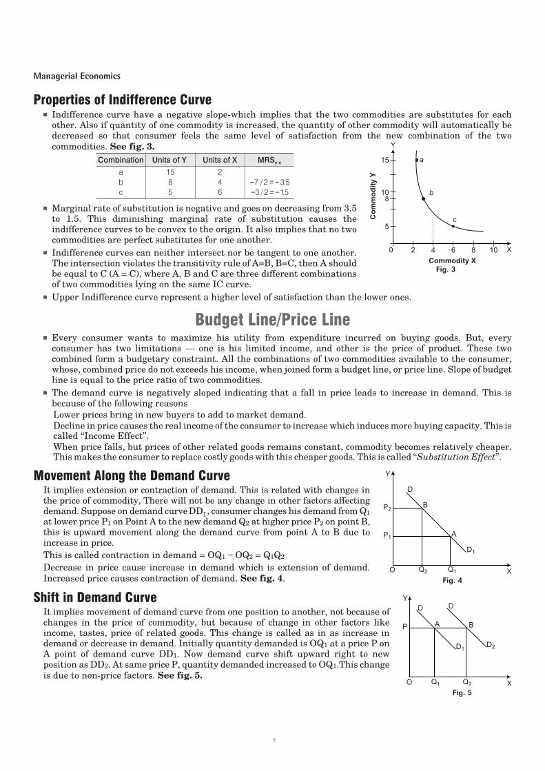
Properties of Indifference Curven Indifference curve have a negative slope-which implies that the two commodities are substitutes for each

other. Also if quantity of one commodity is increased, the quantity of other commodity will automatically bedecreased so that consumer feels the same level of satisfaction from the new combination of the two

commodities. See fig. 3.

Combination Units of Y Units of X MRSy-x

a

b

c

15

8

5

2

4

6

− = −7 2 3 5/ .

− = −3 2 15/ .

n Marginal rate of substitution is negative and goes on decreasing from 3.5to 1.5. This diminishing marginal rate of substitution causes theindifference curves to be convex to the origin. It also implies that no twocommodities are perfect substitutes for one another.

n Indifference curves can neither intersect nor be tangent to one another.The intersection violates the transitivity rule of A=B, B=C, then A shouldbe equal to C (A = C), where A, B and C are three different combinationsof two commodities lying on the same IC curve.

n Upper Indifference curve represent a higher level of satisfaction than the lower ones.

Budget Line/Price Linen Every consumer wants to maximize his utility from expenditure incurred on buying goods. But, every

consumer has two limitations — one is his limited income, and other is the price of product. These twocombined form a budgetary constraint. All the combinations of two commodities available to the consumer,whose, combined price do not exceeds his income, when joined form a budget line, or price line. Slope of budgetline is equal to the price ratio of two commodities.

n The demand curve is negatively sloped indicating that a fall in price leads to increase in demand. This isbecause of the following reasons

Lower prices bring in new buyers to add to market demand.

Decline in price causes the real income of the consumer to increase which induces more buying capacity. This iscalled ‘‘Income Effect’’.

When price falls, but prices of other related goods remains constant, commodity becomes relatively cheaper.This makes the consumer to replace costly goods with this cheaper goods. This is called ‘‘Substitution Effect’’.

Movement Along the Demand CurveIt implies extension or contraction of demand. This is related with changes inthe price of commodity, There will not be any change in other factors affectingdemand. Suppose on demand curveDD1, consumer changes his demand from Q1

at lower price P1 on Point A to the new demand Q2 at higher price P2 on point B,this is upward movement along the demand curve from point A to B due toincrease in price.

This is called contraction in demand = OQ1 − OQ2 = Q1Q2

Decrease in price cause increase in demand which is extension of demand.

Increased price causes contraction of demand. See fig. 4.

Shift in Demand CurveIt implies movement of demand curve from one position to another, not because ofchanges in the price of commodity, but because of change in other factors likeincome, tastes, price of related goods. This change is called as in as increase indemand or decrease in demand. Initially quantity demanded is OQ1 at a price P onA point of demand curve DD1. Now demand curve shift upward right to newposition as DD2. At same price P, quantity demanded increased to OQ1.This change

is due to non-price factors. See fig. 5.


Y

XO

D

D1

P

Q1 Q2

A

D

D2

B

Fig. 5

Y

XO

D

B

A

D1

P2

P1

Q2 Q1

Fig. 4

15

10

5

2 4 6 8 10

Co

mm

od

ity

Y

Commodity X

a

b

c

8

Y

X0

Fig. 3

5

Revealed Preference Theory–By Samuelson

This theory is based on the axiom that all the combination on a budget line are equally expensive, and if a consumer purchases any oneparticular combination. It means his preference for that particular combination is revealed. The consumer reveals his preference by thecombination of goods he buys at different prices. This theory is also treated as the ‘‘Third root of the logical theory of demand’’.

Demand FunctionDemand function sets the relation between the demand and the factors that influence the demand. Demand for acommodity not only depends on the price of a commodity, but also on the income, price of substitutes andcomplementary goods, tastes, habits of consumer.

Short-run Demand FunctionQuantity demanded of X (Dx) depends on prices of X (Px), other factors remain constant in the short run.

Thus Dx = f Px( ). Thus change in Px causes change in Dx.

Long-run Demand FunctionQuantity demanded of X ( )Dx depends on all the factors related to price as well as the consumer.

Dx = f Px I T Ps Pc( , , , , ......),

where, Px = Price of commodity x

I = Income of consumer, T = Taste and preference of consumer

Ps = Price of substitute goods, Pc = Price of complementary goods

Linear Demand FunctionIt is a straight line curve with constant ∆ D/∆ P i.e., change in demand w.r.t change in price is same on the whole

curve. It creates demand line.

Non-linear Demand FunctionIt is a curvilinear shaped curve with ∆ D/∆ P changes along the curve. It creates demand curve.

Law of DemandThis law states that demand for goods increases with the decrease in price for goods, other factors remaining

same.

Elasticity of DemandLaw of demand tells us the effect of changes in price on the demand in terms of increase or decrease but does not

inform about the degree of responsiveness of consumers to a price change. We cannot quantify the change in

demand by studying law of demand.

n Elasticity of demand is the measure of the responsiveness of demand to changing prices. The measure is known

as the elasticity coefficient (Ed).

EQ Q

P Pd =

∆∆

/

/

Types of Demand Curves on Basis of Their Elasticities

Perfectly Inelastic Demand Curven Curve where price change has no effect on quantity demanded. It remains OQ at price OP1 as well as OP2

∆Q = 0. Total revenue decreases with decrease in price.

n Ed = 0. Very essential commodities like medicines, salt, etc have no effect on demand of the change in price.


6

Inelastic Demand Curve

When the price (P) falls, the quantity (Q) increase but at less rate, total revenue

(TR) still decreases. See fig 6.

∆ ∆Q P< , Ed <1

It is also called as relatively inelastic demand curve.

P Q1 1 150 10 5000= = =, , TR

P Q2 2 210 130 1300= = =, , TR

∆Q = 30, ∆P = 40, Ed < 1

Unitary Elastic Curve

It is a case where total revenue remains unaffected by change in price. Changein price will have equal affect on change in demand, so that total revenue

remains same. See fig. 7.

Ed=1

P1 = 100, Q1 = 5, P1Q1 = TR1= 500

P2 = 10, Q2 = 50, P2Q2 = TR2= 500

EQ Q

P Pd = ∆

∆/

/= =45 5

90 101

/

/

Elastic Demand Curve

It has an elasticity coefficient between 1 and ∞, have the property that when

price decreases, revenue increases and vice versa. See fig. 8.

Quantity demanded increases at much greater rate than price decrease.

P1 = 10, Q1 = 50, TR1= 500

P2 = 5, Q2 = 150, TR2= 750

Perfectly Elastic Demand Curve

These are the curves where quantity demanded is infinitely responsive to a

very small price change. See fig. 9.

When price falls, demand increases infinitely, ∆Q→ ∞, ∆ P→0, TR→ ∞When price rises, quantity demanded falls to zero and total revenue falls tozero

∆Q Þ 0, TR = 0

This is a situation where no reduction in price is needed to cause an increase indemand to infinity.

Ed = ∞

Measurement of Elasticity of Demand–By Marshall

% The elasticity can be measured between any two points on a demand curve called arc elasticity or at a point called as point elasticity.

% Method for arc elasticity eQ

P

P

Qp = − ∆

∆. 1

1

% Point elasticity method is used where change in price is infinitesimally small. It is equal to ratio of lower portion below point to the upperportion above point on the linear curve.

eQ

Q

P

Pp = ∂

∂.


P

QO

D

P1

P2

Q1 Q2

D

E > 1d

Fig. 8

P

QO

D

P1

P2

Q1 Q2

D

E = 1d

Fig. 7

P

QO

P1

Q1 Q2

D= ∞

Fig. 9

P

QO

D

P1

P2

Q1 Q2

D

E < 1d

Fig. 6

7

Relation Between Price Elasticity (ep ) and Marginal Revenue (MR)Total revenue TR = P.Q

Marginal revenue MR =∂∂

∂∂

TR

Q

P Q

Q=

( . )

⇒ MR = + = +P Q

Q

Q P

QP

Q P

Q

(

( )

.( )

( )

.( )

( )

∂ )∂

∂∂

∂∂

⇒ MR = P 1 11+

= + −

Q

P

P

QP

ep

.( )

( )

∂∂

⇒ MR = Pep

11−

Relation Between Price Elasticity (eP ) and Average Revenue (AR)Price = Average revenue (AR), P = AR

MR = AR 11−

ep

= AR − AR

ep

⇒ eAR

AR MRp =

−

Price Elasticity of DemandA product with more elastic demand will be fixed at a lower price relative to the

product having inelastic demand whose price can be fixed high. See fig. 10.

EQ

P

P

Qp = ×

∆∆

Income Elasticity of Demand

EQ

Y

Y

Qy = ∆

∆.

Where, ∆Y = change in income. Income elasticity of demand is low for inferiorgoods as with increase in income, consumer will buy less of these goods, andhigh for superior goods.

Cross Elasticity of DemandThe cross elasticity ( )E c is the measure of change in demand for a commodity in response to the changes in theprice of its substitute goods or complementary goods.

EQ

Q

P

Pc =

∆∆

1

1

2

2

.

Where Q1 is quantity demand of product 1 and P2 is price of product 2.

Complementary Goodsn Electricity and electrical machines, butter and bread, pen and ink, petrol and vehicle. Substitute goods can be

vanaspati ghee and desi ghee, tea and coffee, sugar and jaggery, vegetables and pulses.

n The cross elasticity of demand of complementary goods is negative, two goods A & B are complementary to eachother, fall in price of A will lead to increase in demand for B and vice- versa.

n The cross elasticity of demand for substitute goods is positive. The fall in price of coffee will decrease thedemand for tea and vice-versa.

n Cross elasticity defines the relationship between two commodities. If EC is positive and higher the two goodsare very close substitute. If EC is lower in value and negative, the two goods are complementary to each other,but to some extent only.

1 0 UGC-NET Tutor Management

P

QO

D

D1

P2

P1

Q

E = od

Fig. 10

8

n Cross elasticity for two goods cannot be reciprocated. The EC of tea w.r.t coffee is never equal to the EC of coffee

w.r.t tea.

Advertising Elasticity of Salesn The responsiveness of sales to the changes in promotional expenditure can be measured in terms of advertising

elasticity of sales, EA

ES S

A AA =

∆∆

/

/

n Suppose EA= 0.4. It means that the one per cent increase in ad-expenditure results in only 0.4 per cent increase

in sales(s).

n Advertising elasticity (A) lies between zero and infinity. It can never be negative.

Factors That Determine Ad-elasticity aren The level of total sales.

n Advertisement by competitive firms.

n Overall effect of past advertisement.

n Other factors like product's price, consumer's income, etc.

Elasticity of Price Expectationn This concept was introduced by JR Hicks in 1939. Sometimes, consumer decides to buy a good in anticipation of

fluctuations in future price.

n The price-expectation-elasticity ( )Ex , refers to the expected changes in future price, ( )PF , as result of change incurrent prices, (Pc), of a good.

EP P

P Px

f f

c c

=∆

∆

/

/

n Concept of elasticity of price-expectation is very useful in formulating future pricing policy. It is important incase of costly and highly valuable goods.

Demand ForecastingAs defined by ‘Cundiff and Still’, ‘‘Demand forecasting is an estimate of demand during a specified future period

based on a proposed marketing plan and particular uncontrollable and competitive forces.’’

Methods of Demand Forecastingn There are two categories in which demand forecasting methods were classified—survey method and statistical

methods.

n Survey method can be applied to consumer using census or sampling and can also be applied to opinion pollfrom experts using Delphi method.

n Statistical methods can be trend projection methods (least square and graphical methods), barometricmethods and econometric methods (Regression method and simultaneous equations method).

n Least square method is used for projecting trend line. When the time series data shows a increasing trend in

the sales, then a linear trend equation s = a + bt can be used, a and b are constants, t is time period, and s issales in a year.

n Barometric method is based on the work done by National Bureau of Economic Research of US. It is used toforecast general trend in overall economic activities or general business conditions of an industry. Economicindicators used are

d Leading indicators variables which move up and down ahead of other related variables

d Coincidental indicators variables that move up and down simultaneously with economic activity ormarket trends.

d Lagging indicators variables which fall behind other variables.

Managerial Economics 1 1

9

n Barometric method can only be used for forecasting very short run demand. It is generally used to forecastbusiness cycles.

n Delphi method attempts to arrive at a consensus between all experts about the future demand of a product byrepeatedly questioning these experts. Information about opinions of other experts is shared between allexperts. This feedback helps the expert in revising their earlier opinions. This may result in narrowing down ofdifferent views.

Production FunctionIt is the technological relationship between all the inputs and outputs which can be represented in the form of anequation. The production function may take the form of a schedule, a table, a graph or curve, or a mathematicalequation.

Q = f (L, K, M, T, t, LB)

Where, Q = Quantity of output

T = Technology

L = Labour

M = Material

LB = Land and building

t = Time

K = Capital

Short-run PeriodIt refers to a period of time in which the supply of certain inputs, like plant and building, is fixed or is inelastic.Thus, production can be increased by increasing use of variable inputs like man power and raw material.

Short-run Production Function

Supply of capital (K) is inelastic or fixed. It is also called single variable input production function.

Q = f (K, L)

Long-run PeriodA period of time in which the supply of all inputs is elastic, but cannot change the technology. All inputs are variable.

Long-term Production Function

Both K & L can be increased Q = f (K, L)

Very Long-run PeriodRefers to a period of time in which the technology of production is also subject to change or can be improved along

with other inputs.

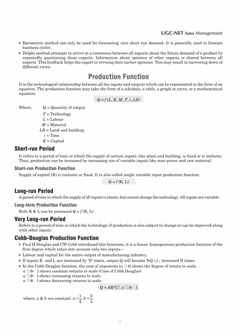
Cobb-Douglas Production Functionn Paul H Douglas and CW Cobb introduced this functions, it is a linear, homogeneous production function of the

first degree which takes into account only two inputs—

n Labour and capital for the entire output of manufacturing industry.

n If inputs K and L are increased by ‘N’ times, output Q will become NQ i.e., increased N times.

n In the Cobb-Douglas function, the sum of exponents (a b+ ) shows the degree of return to scale.

a b+ = 1 shows constant returns to scale (Case of Cobb Douglas)

a b+ > 1 shows increasing returns to scale

a b+ < 1 shows decreasing returns to scale.

Q = AKaLb, a b+ = 1

where, a & b are constant. a = 1

4, b = 3

4


10

Nature of Production Functionn The factors of production are complementary to one another, this is revealed by principle of ‘‘returns to scale’’

where all the inputs are required to be increased simultaneously to attain higher scale of total output.

n The factors of production are substitutes of one another. We can substitute one unit of capital by few units of

labour.

n All inputs are specific to the production of a particular product, none of the factors can be ignored.

Laws of Returns to a Variable InputThis law states that when more and more units of a variable input (labour) are used with a given quantity of fixed

input (capital), the total output may initially increase at an increasing rate, then at a constant rate but finally it

increases at ‘‘Diminishing’’ rate. Thus, marginal increase in total output decreases when more and more units of

a variable factor are used, given the state of technology and fixed factors.

Assumptions of Law of Diminishing Returnsn Labour is the only variable input.n All other factors remain same.

n Labour is homogeneous.n State of technology is fixed.

n Input prices are given.n In the words of Prof Samuelson, an increase in some inputs, will, in a given state of technology, cause output to

increase but after a point the extra inputs will become less and less effective.’’

n These extra inputs are surplus labour whose marginal productivity eventually declines.

n Total Product (TP) increases initially at an increasing rate till the marginal product is also increasing, it isfirst stage (increasing returns). Once the marginal product declines, the total product starts increasing at adecreasing rate. This is the stage of diminishing returns (second stage).

n When Marginal Product (MP) becomes zero, total product is at maximum level. After word, MP becomesnegative, TP started declining. This is the (third stage) stage of negative returns.

n When MP = AP, Average Product is at its maximum.

When MP= 0, TP is at its maximum.

When MP<AP, AP starts declining.n Point of inflexion is the level at which MP is maximum. Till the point of inflexion, TP curve increases sharply.

Iso-Quant CurveIt can be defined as the locus of all those points representing various combinations of two inputs—capital and

labour yielding the same level of output. It is also called as ‘‘Equal Product Curve” or ‘‘Production. Indifference

Curve’’. When both these inputs can be changed in long run, relationship between inputs and outputs can be

explained by laws of returns to scale’’.

Assumptions of Iso-quant Curvesn There are only two inputs labour and capital.n Both inputs are perfectly divisible.n Both are imperfect substitutes for each other.n Technology of production is constant.

Iso-quant IQ1 See fig. 11 represent various input combinations producing 50units of output

Points K L Output

A 60 10 50

B 40 15 50

C 20 20 50

20 units of capital are being substituted by 5 units of labour when we go from point A to B.


60

50

40

30

20

10

0

A

B

C IQ = 1002

IQ = 501

10 15 20

Labour

Ca

pit

al

K

L

Fig. 11

11

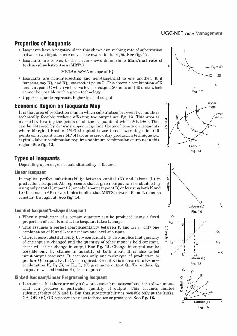
Properties of Isoquantsn Isoquants have a negative slope-this shows diminishing rate of substitution

between two inputs curve moves downward to the right. See fig. 12.

n Isoquants are convex to the origin-shows diminishing Marginal rate of

technical substitution (MRTS)

MRTS = ∆K/∆L = slope of IQ

n Isoquants are non-intersecting and non-tangential to one another. It ifhappens, say IQ1 and IQ2 intersect at point C. This shown a combination of Kand L at point C which yields two level of output, 20 units and 40 units whichcannot be possible with a given technology.

n Upper isoquants represent higher level of output.

Economic Region on Isoquants MapIt is that area of production plan in which substitution between two inputs istechnically feasible without affecting the output see fig. 13. This area ismarked by locating the points on all the isoquants at which MRTS=0. Thiscan be obtained by drawing upper ridge line (locus of points on isoquantswhere Marginal Product (MP) of capital is zero) and lower ridge line (allpoints on isoquant where MP of labour is zero). Any production technique i.e.,capital - labour combination requires minimum combination of inputs in this

region. See fig. 13.

Types of IsoquantsDepending upon degree of substitutability of factors.

Linear Isoquant

It implies perfect substitutability between capital (K) and labour (L) inproduction. Isoquant AB represents that a given output can be obtained byusing only capital (at point A) or only labour (at point B) or by using both K andL (all points on AB curve). It also implies that MRTS between K and L remains

constant throughout. See fig. 14.

Leontief Isoquant/L-shaped Isoquantn When a production of a certain quantity can be produced using a fixed

proportion of both K and L the isoquant takes L shape.

n This assumes a perfect complementarity between K and L i.e., only onecombination of K and L can produce one level of output.

n There is zero substitutability between K and L. It also implies that quantityof one input is changed and the quantity of other input is held constant,

there will be no change in output See fig. 15. Change in output can bepossible only by change in quantity of both input. It is also calledinput-output isoquant. It assumes only one technique of production toproduce Q1 output, K1, L1 (A) is required. Even if K1 is increased to K2, newcombination K2 L1 (B) or K1, L2 (C) give same output Q1. To produce Q2

output, new combination K2, L2 is required.

Kinked Isoquant/Linear Programming Isoquantn It assumes that there are only a few process/techniques/combinations of two inputs

that can produce a particular quantity of output. This assumes limitedsubstitutability of K and L. But this substitutability is possible only at the kinks.

OA, OB, OC, OD represent various techniques or processes. See fig. 16.


IQ = 402

IQ = 201

CK

L

Fig. 12

a

d

b

e

f

c

upperridge

lowerridge

K

LO Labour

Ca

pit

al

Fig. 13

Y

XLabour (L)

Ca

pit

al(K

)A

BO

Fig. 14

Y

XLabour (L)

Ca

pit

al(K

)

a

b

c

d

A

B

C

D

O

Fig. 16

X

Labour (L)

Ca

pit

al(K

)

K2

K1

L1 L2

B

A

C

Q1

Q1

Y

O

Fig. 15

12

n By joining kink points a,b,c,d, we get Kinked isoquant. It is also called the ‘‘linear-programming isoquant’’

or ‘‘activity analysis isoquant’’.

n Kink are the technical feasible points.But on normal isoquant curve, all points are technically feasible for production.

Smooth, Convex Isoquantn This form assumes continuous substitutability of capital (K) and labour (L) only over a certain

range, beyond which factors cannot substitute each other. The Isoquants appears smooth and

convex to origin. See fig. 17.

Isocost Line/Price Line/Outlay Linen It indicates different combinations of two factors of production which a firm

can purchase at given prices with a given cost.

n As the cost of factors increases, Isocost line moves right upward. A producer isin the state of equilibrium at point Q at which Isocost line AB touchesisoproduct curve IP. Point Q is the optimum factor combination which

produces output at minimum cost also known as Least Cost Combination(LCC). See fig. 18.

Production Possibility Curve (PPC)n Producer has limited factors of production and they can be put to various

uses for producing various commodities. So, these factors or inputs can beused in a way to produce various combinations of goods. These

combinations of two commodities are termed as ProductionPossibilities (PP) and the curve joining these PPs is known as

Production Possibility Curve (PPC). Thus, we can explain using chart.

PPs Production of TV Production of Fridge

A 0 30

B 10 25

C 15 20

D 25 10

E 30 0

Four PPs are shown of PPC curve AE. See fig. 19.

n Production possibility curve slopes downwards to the right and is concave to the origin. It implies that forproduction of additional units of goods on X-axis, increasing quantities of goods on Y-axis will need to besacrificed. It is assumed that the time period is short and production technique is constant.

First Order Condition for Least Cost Combination (LCC)Can be expressed as : Ratio of Marginal Productivity (MP) of two factors should always be equal to the ratio of

prices (P) of these two factors of production

L = labour, K = capitalMP

MP

P

P

L

K

e

k

=

Second Order Condition for LCCAlso called as supplementary condition. It requires that the first order condition be fulfilled at the highest

possible isoquant.

Laws of Returns to ScaleIt explains the behaviour of output in response to proportional and simultaneous change in all the inputs. This

can be possible in long-run when production capacity can be increased beyond its maximum limit by increasing

fixed as well as variable factors of production. This is an expansion of scale of production.


Y

X

I

Q

L

K

Fig. 17

30

25

20

15

10

5

0

D

C

5

Fridge

TV

Y

X10 15 20 25

A

B

E

30

Fig. 19

Y

XLabour (L)

Ca

pit

al(K

)

A

B

Q

IP

Fig. 18

13

Increasing Returns to ScaleWhen output increases more than proportionately to the increase in inputs. Suppose if on doubling the inputs,output increases more than double, it exhibits increasing returns to scale. Marginal product is always greaterthan the average product. MP>AP

Causes for Increasing Returns to Scalen Indivisibility of factors of production like machines and managers. If scale is increased, capabilities of a

manager as well as the machine can be fully utilized. This is application of managerial economies.

n Higher degree of specialization increases productivity of both labour and machinery.

n Financial economies of buying in bulk reduces the transportation cost as well as purchase prices can benegotiated when volume is large.

Constant Returns to ScaleWhen output increases in the same proportion to the increase in inputs, it exhibits constant returns to scale.Average product and marginal product will not change and will remain same at all levels of production MP=AP.The constant returns are the result of limits of economies of scale. Once the factors of production reached itsoptimum level, production cannot be increased beyond this limit, it will stagnate. This production function ishomogeneous of degree 1, capital-labour ratio is fixed.

Decreasing Returns to ScaleIt applies when a certain proportionate increase in inputs leads to a less than proportionate increase in output.This can be explained as when capital and labour are increased by 50% the output increases by only 40%. In thiscase marginal product is always less than average Product MP<AP. It implies total product is increasing atdiminishing rate.

MP = 0, when TP is maximum.

Types of Costs

Explicit CostAre the money expenditure incurred on the resources used in the production of a commodity. These are alsoknown as paid out costs, expenditure costs and also as outlay costs.

Implicit Costn Are the costs of self-owned and self-employed resources, which if employed else-where were being paid. These

include interest on capital employed by entrepreneur in his firm, rent of building owned by entrepreneur,reward for his managerial skills. These are non-expenditure costs also called as imputed cost. Opportunity costis an example of imputed cost.

n The explicit and implicit costs together make the economic cost.

Social CostThese are the costs that arise due to the production of the firm but they are not borne by the firm but they areborne by the society. This cost includes (i) the use of natural resources freely available, and (ii) the dis-utilitycreated in the process of production. These cost together constitute social cost, also termed as external costs.Example is the chemical factories discharging its waste in rivers, air pollution created by chimneys of the firm,etc. Resources used are atmosphere, rivers, land etc.

Real CostEfforts, pains and exertions of labour along with wait and abstinence required by entrepreneur for saving thecapital used in making a commodity. It is a subjective type of cost introduced by Marshall.

Incremental CostIncrease in total cost on an increase in the level of operations is called the incremental cost. This cost isassociated with the decisions to expand the output or to add a new variety of product or to replace worn out plantand machinery. It is also termed as differential cost and it does not apply to a new firm but applies to existingfirm only.


14

Fixed Cost (FC)Are costs incurred on production firm which is fixed in short-run irrespective of the volume of output level. These areincurred even if production comes to hault. These include office over heads, depreciation on machinery, building,maintenance of firm etc. Fixed costs are also known as general costs, supplementary costs and indirect costs.

Variable Cost (VC)Also known as prime costs or direct cost, it varies with the variation in the volume oftotal output. It includes cost of raw material, running cost of fixed capital, directlabour charges and costs of all other inputs that vary with output.

Total Cost (TC)It is the sum of fixed costs and variable cost. TC = FC + VC

Total cost curve TC moves parallel to total variable cost curve (TVC)

because difference between TC and TVC is FC which remains constant. See fig. 20.

Average Variable Cost (AVC)AVC declines at initial stage due to law of increasing returns. It becomes constant

when firm attains its full capacity, AVC starts to increase due to application of law of

diminishing returns. Thus, AVC gets ‘U’ Shape in long-run. Same is applicable to

Average Cost Curve. It is also U shaped. See fig. 21.

Types of Cost Functions

Short-run Cost FunctionsThe shape of the short run cost curves depends on the type of cost functions like linear, quadratic or cubic

functions.

Linear Cost Function

TC = a + bQ

a = TFC, b = change in TVC = MC,

Q = quantity produced

MC =∂∂TC

Q= b.

MC remains constant throughout in case of a linear function. see fig. 22.

Average cost and marginal cost curves can be presented as.

Average cost continues to decline with the increase in output.


Y

X

Co

st

OutputO

TC

FC TVC

Fig. 20

Y

X

AV

C

OutputO

Fig. 21

Y

X

Co

st

OutputO

TC

TVC

TFC

a+bQ

bQ

a

Fig. 22Y

X

Co

st

OutputO

ACMC

15

Quadratic Cost Function

TC =a + bQ + Q2 , AC =a

Q+ b+Q, MC= b + 2Q

where a,b are constants, Q is total output, TC is total cost.

Cubic Cost Function

TC = a + bQ + CQ2 + Q3 , AC =TC

Q=

a

Q+ b + CQ + Q2

where, a, b and C are constants

MC = = + +∂∂TC

2C 3 2

Qb Q Q

Relation between MC and AC Curven Both AC and MC are derived from total cost. So as far as AC falls, MC falls

more sharply MC < AC.

n MC curve cuts AC curve from below at the minimum. This is point ofoptimum capacity.

n When AC increases, MC also increases but at a more pace, i.e., MC > AC

after intersection. See fig. 23.

n MC reaches its minimum level sooner than AC.

n Thus, just before the point of intersection, MC must be rising while AC isfalling but MC curve must be below the AC curve.

Long-run Cost CurveLong-run is a period characterised by changing factors of production, fixed as well as variable.

The firm plans to produce more by building a new large plant by changing the

production technique. See fig. 24. Laws of return to scale applies

n Each plant capacity has its own Short-run Average Cost Curve (SAC). In

long-run, there can be a large number of plants as well as their SACs.

n LAC curve is a U shaped curve enveloping all the SACs. LAC curve is flatter,smooth and is tangent to all the SAC at its minimum point. It is also calledenvelope curve.

n Long-run Average Cost Curve (LAC) helps the firm to determine anoptimum scale of operation which incurs least cost and maximum profit.

Characteristics of LAC Curven LAC curve can never intersect or cut a SAC curve though they are tangential to each other. This implies that

for any given output, average cost cannot be higher in the long-run than that in the short-run.

n If law of constant return applies to industry, LAC curve can be a horizontal line. In this case, point of minimumcost of all SACs will be equal.

n LAC is always lower than SACs because costs can be reduced only in the long run.

Break-even AnalysisFor any firm to operate, there is a level of output, below which production is non-profitable or may be in loss, andabove which the firm starts earning profit,. Break-even analysis helps the firm in determining this break evenpoint at which firm is at par i.e., revenues are equal to costs and no-loss no-profit situation has arrived.

Break-even analysis, also known as Cost-Volume-Profit analysis is a technique to study the relationshipbetween the total costs, total revenue and total profits or losses over various levels of output.At break-even point TR = TC


Y

X

Co

st

OutputO

MCAC

Fig. 23

Y

X

Av

era

ge

Co

st

OutputO

SAC1 SAC2

SAC3

SAC4

Fig. 24

16

Relation between Break-even Volume and Price

TR = TC = TFC + TVC

TVC = AVC × Qb

TR = P × Qb ⇒ P × Qb = TFC × AVC × Qb

Qb (P − AVC) = TFC

Qb =TFC

AVCP −=

−TFC

MCP

Where, TFC = Total Fixed Cost, P = Unit Price, AVC= Average Variable Cost = MC

Qb = Break Even Volume.

Break-even ChartAt point B, TR curve and TC curve intersect. At OM level of output, totalcost equals total revenue. Thus, B is the break even point. Below point B,TC curve is above TR curve showing losses. Above B, TR curve is higherthan TC curve implying profits. See fig. 25.

Assumptions of Break-even Analysisn All costs can be separated into fixed and variable costs.n Selling price will remain same throughout the operation though there

may be competition or change in volume of production.n There will not be any opening or closing stock .n There will not be any change in technology of production.

Relation Between Break-even Point and P/V Ratio

Break even point (in sales) = ×−

Fixed Cost Selling Price

Selling Price Variable Cost= ×

−F SP

SP V

P/V Ratio =SP VC

SP

−

BEP (in sales) =Fixed cost

P / V Ratio

Margin of Safety (MoS)It is the difference between actual sales and the break even point sales. It is the range of sales over and above thebreak even sales. If the difference is big, it implies that the firm can still make profits even after a serious drop inproduction

MoS = Present sales − Breakeven sales = =

Profit

P / V ratio(Profit) /

Contribution

Sales

Unsatisfactory margin of safety can be improved by increasing the level of production, increasing the sellingprice, reduces the total cost of production and by substituting the current products by more profitable productswhich can be produced by the firm.

Market StructuresThe number of sellers of a product in a market determines the type of market and degree of competition in themarket.

Depending on the number of sellers, market structure is divided into four categories

n Cat. 1-Perfect competition n Cat. 3-Monopolistic competition

n Cat. 2-Oligopoly n Cat. 4-Monopoly


Y

XC

os

t&

Re

ve

nu

eOutput

O

OperatingLoss

angleof incidence

Profit

TR

TC

TVC

TFC

B

M

Fig. 25

17

Perfect CompetitionAccording to Prof Ferguson, ‘‘Perfect competition describes a market in which there is complete absence of

direct competition among economic groups.’’

Perfect competition is characterised by the presence of large number of firms selling homogeneous products with noproduct difference like farm production and financial market products.

Features of Perfect Competitionn Great number of buyers and sellers, no one is capable of affecting the price in the market.n Free entry and free exit for all buyers and sellers in the perfect competition market.n Homogeneous products are identical and perfect substitute.n All buyers and sellers have perfect knowledge of prices.n All firms enjoy easy access to the market. There is absence of any transport cost which differentiates the price.n Absence of government or artificial restrictions on the working of the firms.

n Pure competition It is the perfect competition with no perfect mobility of factors and with no perfectknowledge.

Pricing Under Perfect Competition

Price is determined by the laws of supply and demand. Price will be fixed at apoint where the market demand and market supply are at an equilibrium.Demand is governed by the law of demand based on marginal utility of thecommodity to the buyers. Supply is governed by the cost of production. Point atwhich the market demand equals to the market supply, that is the point of

equilibrium. See fig. 26.

DD′ is the market demand curve and SS ′ is the market supply. Both curvesintersect at point E. PE is the equilibrium price of the industry.

Price Elasticity of Demand for an Individual Firm in a Perfect Competition

It is infinite. Demand curve will be a horizontal straight line at the particularprice level as firm can sell infinite quantity of product at prevailing price in the

market. There is no degree of control over the price by any single firm. See fig. 27.

In perfect competition, MR = AR = MC = P

firm makes normal profit. If AR > AC, then only firm makes economic profit.

Pure MonopolyIt means an absolute power of a firm to produce and sell a product that has no closesubstitute in the market. The cross elasticity of demand for a monopoly product is eitherzero or negative. Firm and industry are identical in a monopoly competition.

1. A natural monopoly may emerge out of the technical conditions of efficiency and economies of scale.

2. There is no certainty that a monopoly firm will always earn an economic profit. This all depends on

d its cost and revenue conditions.

d threat from potential competitors.

d government policy in respect of monopoly.

Profit of Monopoly Firms

If AR > AC, firm enjoys supernormal or economic profit.

AR = AC, firm enjoys normal profit.

AR < AC, firm makes losses.

Measure of Monopoly Power

JS Bains and AP Lerner have used ‘‘Excess Profit’’ criterion for calculating the monopoly power of a firm. Excessprofit can be defined as the profit in excess of the opportunity cost. While calculating excess profit, theopportunity cost of owner's capital and a margin for the risk must be deducted from the actual profit made by thefirm.


Y

X

Pri

ce

OutputM

D

S D′

S′

EP

O

Fig. 26

Y

X

Pri

ce

QuantityO

Fig. 27

18

(i) JS Bains formula

Monopoly power =R O

R

−

where, R = actual profit O = opportunity cost

If (R− O) / R= 0, there exists no monopoly, and if this ratio is greater than zero, there is monopoly. The highervalue of (R-O)/R, the greater is the degree of monopoly.

(ii) AP Lerner formula

Monopoly power =P MC

P

−

where, P = Price, MC = Marginal Cost

For a profit maximizing firm, MC = MR, P= AR

Monopoly power =P MR

P

− = 1

e

Lower the elasticity, greater the degree of monopoly. Even if AR=AC and firm earns only normal profit, monopolypower still exists.

Monopolistic CompetitionIt is a market setting in which many firms sell differentiated products. Differentiation is made by way ofdifferent brand names, trade marks, designs, colours, shapes, packaging, qualities, etc.

But, still each product is a close substitute for the rival products. Each firm enjoys a quasi-monopoly over itsproduct. Examples are movie theaters, FMCG products, dresses, restaurants, consumer durables. This isperceived difference in the minds of customers.

Price Determination in Monopolistic Competitionn Edward H Chamberlin developed a model for determining equilibrium price. Chamberlin's analysis shows

that price competition results in the loss of monopoly profits. All the firms will be looser and no one can gain.He finds out two ways to non-price competition—

(i) Product innovation (ii) Advertisement

n In monopolistic competition selling cost includes cost on research and development, free sampling, tradediscounts to dealers, free scheme for customers, media ads. Sales increases initially at increasing rates buteventually it decreases. Thus, average selling cost curve initially decreases but ultimately it increases.Therefore, the Average Selling Cost curve is U shaped similar to AC curve.

n Non-price competition through these selling cost leads all the firms to an almost similar equilibrium whichChamberlin calls it as ‘‘Group-Equilibrium’’.

n Price elasticity of demand in monopolistic market is large.n Two conditions for the firm’’s equilibrium under perfect competition are MC = MR = Price,

slope of MC curve > slope of MR curve

n The firm will continue to produce only if it covers its variable costs. The point at which the firm covers itsvariable cost only is called ‘‘closing-down point’’. If sale is below this output level, firm will incur losses.

OligopolyThis competition is characterised by few firms or sellers selling homogeneous or little differentiated products.The number of sellers is so small that the market share of each firm is large enough for a single firm to influencethe market price. Examples are- mineral water, cigarettes, aluminum, steel, cement industry.

Barriers to Enter Oligopolistic Marketn Huge investment requirements to match the production capacity of existing firms.n Strong customer loyalty.n Preventing entry of new firms by price war. Mostly MNCs and big corporate houses can enter oligopolistic

market.


19

Augustin Cournot Model

He was the first economist to develop a formal oligopoly model in the form of a duopoly model with two firmsdealing in mineral water business.

This model assumes duopoly of two firms operating at zero cost, both of them are facing a demand curve with aconstant negative slope. According to this model, profit is maximum when MC = MR = 0 and profit maximizingoutput is half of the total market demand i.e., Q/2.

Types of Oligopolies

Partial oligopoly It refers to that market situation where the industry is dominated by one large firm whichis looked upon as the price leader. Rest firm decides their price on the basis of this leader.

Full oligopoly It is that market situation where there is no price leadership.

Perfect/ Pure oligopoly If the firms are producing homogeneous products. e.g., aluminium industry.

Imperfect/differentiated oligopoly When competing firms produce imperfect close substitutes which aresomehow differentiated. Example mineral water industry.

Syndicated oligopoly Situation where the firms sell their products through a centralised syndicate. This

syndicate fixed prices and output quotas for all firms.

Collusive oligopoly Refers to that market situation where the firms, instead of competing, combine togetherto fix price. This body is termed as a cartel.

Non-collusive oligopoly Lack of agreement among the firms.

Economic Impacts of Oligopoly Marketsn High selling cost due to aggressive sales promotion efforts as in the case of Pepsi and Coke.

n Economies of scale cannot be achieved leading to higher costs.

n Price is higher than average cost and marginal cost.

Kinked Demand Curven This model of oligopoly was developed by Paul M Sweezy and by Hall and Hitch in the same year 1939. The

analysis of kinked demand curve bring out one fact about oligopoly market. See fig. 28.

n Price and output once determined tends to remain same even if there is a considerable change in the cost ofproduction. It does not deal with price and output determination.

n Logic behind sticky price of a firm is that Sweezy believes if a firm reducesthe price, rivals would follow price cuts and neutralise expected benefitsfrom price cut. In case it raises price, other firms may maintain their priceor may even reduce it. In this case price rising firm looses its market share.In both cases, price changing firm lose. Thus, it tends to stick to one price.

n The demand curve facing an oligopolist (in case of differentiated products)has a ‘kink’ at the level of prevailing price. This kink is formed because thesegment of demand curve dK above prevailing price level KM is highlyelastic and the segment of demand curve below prevailing price level isinelastic. A kinked demand curve dD with a kink at point K has beenshown. The prevailing price level is KM and the firm is producing andselling output OM. This difference in elasticities between dK curve and KDcurve is due to the particular competitive reaction pattern assumed bykinky hypothesis. This hypothesis assumes that when a firm raises its price, all customers would not leavebecause some customers are intimately attached to it due to product differentiation. Thus, demand curve willnot be perfectly elastic.

MonopsonyIt is also termed as buyer’s monopoly. Monopsony refers to a market situation when there is a single buyer ofa commodity or service. The monopsonist can influence the supply price of his purchases by the amount he buys.The monopsonist regulates his purchases in such a way that MC = MU whereby his consumer’s surplus is the

maximum.


Y

X

Pri

ce

QuantityM

Q

O

D

K

d

Fig. 28

20

Bilateral MonopolyIt refers to a market situation in which a single producer or seller (monopolist) faces a single buyer(monopsonist). Equilibrium price can be determined by non-economic factors such as bargaining power,

negotiation skills, etc.

Price DiscriminationRefers to the practice of a seller of selling the same goods at different prices to different markets. This variationin prices does not reflect variation in costs in two markets. It is practiced in order to maximise profit.

Necessary conditions for Price Discriminationn Different markets must be separable for a seller to be able to practice discriminatory pricing. Separation can be

on the basis of geographical distance involving high cost of transportation, exclusive use of the goods.

n Elasticity of demand for the product must be different in different markets.

n There should be imperfect competition in the market in the form of monopoly.

n Profit maximizing output must be much larger than the quantity demanded by any one market.

Degrees of Price DiscriminationProf AC Pigou has proposed three degrees of price discrimination on the basis of the extent to which a seller canextract consumers's surplus of the consumers.

First Degree Price Discrimination

It is also termed as perfect price discrimination. It is possible when the market size is small and monopolistknows the highest paying capacity of his buyers. Monopolist sets the price at highest level to extract entireconsumer’s surplus. Then, he lowers down the price of further units to extract consumer’s surplus till last unitconsumed. This can be done through auction sale.

Second Degree Block Pricing

Block pricing or second degree price discrimination is feasible where market size is very large. Monopolistdivides the whole market into three blocks—higher income group, middle-income group and lower income group.He intends to siphon off only the major part of the consumer’s surplus. A single rate is applicable to a largenumber of buyers within a block.

Third Degree Price Discrimination

Third degree price discrimination may be practised between any two or more markets, separated from each otherby geographical distance, transport barriers, legal restriction or inter-regional transport. Two markets must

have different elasticity of demand.

Pricing TheoriesIn a complex business world, the business firms have to consider various factors while deciding the price for aproduct. There can be several strategies that can be adopted by a firm for deciding price like

n Cost-plus pricing n Multiple product pricing

n Pricing in life-cycle of a product n Transfer pricing

Cost-plus Pricingn This is also known as “mark-up pricing”, “average cost pricing” and “full cost pricing”. This is the most

common method of pricing used by the manufacturing firms. This method is based on the average variable costof output which can be estimated for a given period of time, usually one fiscal year in which ‘Q’ output isproduced

AVC =TVC

Q


21

n A “ mark-up’’ is fixed on this AVC which will be the profit margin. Suppose m = mark-up percentage, then price

‘P’ is calculated as P = AVC + m (AVC)

P = AVC (1 + m) = MC (1 + )m

(If MC is constant, MC = AVC)

Multiple Product PricingIn actual practice, no firm can produce a single homogeneous product. Almost all firms produce a commodity inmultiple models, styles and sizes, each so much differentiated from the other that every model or size of productcan be taken as a new product. Each product has different AR and MR curves and that one product of the firmcompetes against the other product of same firm. The pricing under these conditions is known as multi-productpricing or product-line pricing. Since all the products are produced under one production facilities, they have onejoint marginal cost curve but different AR and MR curves. If we sum-up, the intersection of combined MC curveand aggregate MR curve determines the output level and price for each product of the firm.

Pricing in Life-cycle of a ProductIn the words of Kotler and Armstrong, “Product life cycle is the course of a products’ sales and profit over its lifetime.” How the product has performed in the market from introduction period to the declining period. A product

passes through five stages. See fig. 29.

IntroductionStage of launching the product in the market. This is a trial phase withconstant sales.

GrowthProduct gains popularity and sales increasing at fast pace due tocummulative effect of advertisement over the initial stage.

MaturityStage in which sales continue to increase but at a lower rate and the totalsale tends to stabalize.

SaturationPhase in which sales have reached their peak the total sale saturates there is no considerable increase ordecrease in the sales.

DeclineThis is the last stage in which sales begin to decline due to various reasons like availability of substitutes, loss of

product uniqueness, change in fads and fashion, etc.

Pricing for a New Product

Skimming PricingThis strategy is adopted where close substitutes of a new product are not available. In this policy, firm intends toskim the consumer’s surplus off the market by setting a price initially high, then subsequent lowering of prices ina series of reduction . Initial high price should be accompanied by heavy sales promotion, distinct features of theproduct and demand is relatively inelastic.

Penetration Price PolicyThis policy is implemented in case of new products which have close substitutes available in market. This policyrequires fixing a lower initial price designed to penetrate the market as quickly as possible. As the product

catches the sales in the market, price is gradually increased. It requires the demand elasticity greater than one.Economies of large-scale production should be available to the firm. Cross elasticity should be high forsubstitutes.

Veblen Effect

Also termed as demonstration effect, when the consumers are ready to buy goods of prestige at a very highprice. This effect can be seen in malls.


Y

X

To

talS

ale

s

TimeO

Introduction

Decline

Growth

Saturation

Maturity

Fig. 29

22

Transfer Pricing

The goods and services produced by one division of a company is used by the other division of the same company

for further production. In other words, parent division buys the product of its subsidiaries. There will be aproblem of determining an appropriate price for the product transferred from one division to the parent body.Pricing of intra-firm ‘transfer product” is referred to as “transfer pricing’. This technique was provided byHirshleifer. It was assumed that both parent and subsidiary companies have their own profit functions tomaximize and firm has option to sell its product completely in external market and/or to transfer it to the parentcompany.

n The correct transfer price for an intermediate product for which there is no external market is the MarginalCost (MC) of production.

n When a perfectly competitive external market exists, the transfer price for intra-company sales of theintermediate product is given by the external competitive price for the intermediate products.

n When an imperfect market exists, the transfer price is given at the point where the net marginal revenue of themarketing division of the firm is equal to the marginal cost of production division at the optimum level ofoutput of the intermediate product.

AdvertisingAdvertising is any paid form of non-personal communication by an identified sponsor. Aim is sales promotion ofgoods and services to the mass customer.

Objectives of Advertisingn To create awareness and to tell the customers about utility of product.n To persuade the customer, to convince the customer for buying.n To remind and stimulate repeat purchase.

n To convince current customers that they are precious to the company.n Advertising shifts the demand curve to the right and makes the demand

curve less elastic.n In the initial stages of advertisement outlay, the resulting increase in

sales will be more than proportionate to the increase in advertisementexpenditure. Beyond that point, rate of increase in sales decline. Finally, astage will come where the sales become saturated and advertisement hasno effect.

Advertisement Elasticity of DemandIt measures the change in sales volumes (Q) in response to the change in advertising expenditure (A)

EQ Q

A Aa = ∆

∆/

/=

−÷

−S S

S

P P

P

1 2

1

1 2

1

, P1 and P2 are two advertisement expenditures corresponding to S1 and S2

sales volume See fig. 30.

Factors That Influence Advertising Elasticityn Stage of the product in market i.e., if it is a new product or if few substitutes already exists.

n Period of advertisement i.e., for how many days advertisement is done.

n Advertising by rival firms.

Capital Budgetingn It refers to the process of planning capital projects, raising funds and efficiently allocating resources to those

capital projects which are expected to generate returns for more than one year. These include setting up newplants, installing machines, purchase of heavy vehicles and trucks, purchase of IT products for officeautomation, expenditure on R and D work for product innovation. Expenditure on advertisement for longperiod can also be the part of capital expenditure.


Y

X

Sa

les

Advertising Expenditures ( )`

O

S1

S2Totalsales

P1 P2

Fig. 30

23

Decisions Taken in Capital Budgeting aren How much money to be raised, fund requirement?n What could be the source of finances?n Allocation of the money between different projects over a time period.

Types of Investments in Capital Expendituren Investment for replacing worn out machines.n Investments on cost reduction by way of bringing new technology, buying more advance machines, training of

manpower.n Investment for expansion of plant capacity in response to increasing demand.n Investment for introducing new products and to enter new market.n Investment for complying with government regulations like safely hazards, waste management and social

responsibility.

Capital Expenditure is IrrevocableOnce an investment is made in some project, it cannot be converted into cash without a loss. The very survival ofthe firm depends on planning of capital expenditure. Thus, only profitable projects must be selected for goodreturns on investment.

Methods for Evaluating Investment Returns

Pay Back Periodn This method is also called as payout method, calculates the total time period (in number of years) required to

return the original investment. From this, the firm can findout the time period in which it can recover itsinvested funds. It does not take into account depreciation on the machines.

Pay Back period = Total Investment

Net cash Inflows per year= X year

Net cash inflows = Gross profit − (tax + depreciation)

n In case of projects yielding cash inflow in varying amounts, pay-off period can be obtained throughcummulative total of annual returns.

For Example Total fixed outlay is ` 20 Lacs, which yields cash flows over 6 years as shown in following Table

YearTotal Fixed Outlay

(` In Lacs)Annual Cash-Flows

(` in Lacs)Cummulative Cash Flows

(` In Lacs)

1st 20 2 2

2nd – 5 7

3rd – 6 13

4th – 7 20

5th – 6 26

6th – 8 34

From above table we can see that the pay-back period is 4 years as in 4 th year, cummulative cash inflow equateswith total outlay of ` twenty lacs.

Net Present Value MethodThis method is based on the concept of time value of money. A money expected to be received one year later is lessvaluable than the same amount received today. This is due to the fact that we can earn interest on the money inhand in that time period.

Present value + Interest in 1 yr = Future value in 1 yr

FV PV= +( )1 r t

where, r = rate of interest

t = time period in yr


24

PV FV=+

1

1( )r t

where, FV = Future value

PV = Present value

PV FV= × (discounting factor)

Thus, present value of future income can be expressed as its value discounted at the current rate of interest.

For Example If we are going to receive ` 1100 after one year and the rate of interest is 10% per year.

PV =+

= =11001

1 01

1100

111000

1( . ) .

Thus, present value of ` 1100 is ` 1000

In case of different annual returns (R) over n year with ‘r’ rate of interest , total present value of an income streamcan be calculate as

TPV =+

++

++

R

r

R

r

R

r

1 2

2

3

31 1 1,

( ) ( ).... +

+R

r

n

n( )1

TPV = Rr

n ni

n 1

11 ( )+=∑

n Net present value NPV = TPV – Cost of investment

NPV TPV= −C

If NPV > 0, project is acceptable;

If NPV =0, project can be accepted or rejected

If NPV<0, project should be rejected.

Internal Rate of Return MethodThis method is also called “discounted rate of return” or “time adjusted rate of return’’ method. Also termed as

“Marginal efficiency of investment” and “Break-even rate”.

This is the rate of return which equates the total outlay on project with the total net present value of annualcash inflows.

R

rCn

ni

n

( )11 +=

=∑

n IRR method says that so long as internal rate of return is greater than the market rate of interest, it is alwaysprofitable to borrow and invest.

Average Rate of Return MethodThis method does not consider time factor. Average Return of Investment (ARI) is defined as the ratio of netaverage annual income from the project to the initial investment.

n Net average annual income can be calculated by dividing the total annual income of all years by the number ofyears of inflow.

ARI =

∑ R

C

n

i

n

o

=1

/ n

where, Co = initial cost of project.

Rn = annual return in nth year

n = total number of years


25

Average Rate of Return in Percentage

ARR = ×Average Return

Average Total Cost of Project100

In this method the rate of return on investment is calculated without considering time factor.

ARR = Average annual income after Tax and Depreciation

Average investment

= Annual cash inflow after Tax – Depreciation

Initial Investment + Salvage

2

× 100

For example, there is an initial outlay of ` 20000. Annual cash flow after tax but before depreciation is ` 3000 forfirst five years and ` 2000 for next five years. Estimated life is 10 years and salvage is ` 2000. Calculate averagerate of return.

Solution Average annual cash inflow after tax = × + × =5 3000 5 2000

10` 2500

Depreciation = = =Initial outlay

Lift Period

20000

10

,` 2000

Average investment = + =20000 2000

2

,` 11000

ARR = × =2500 2000

11000100 45

–. %

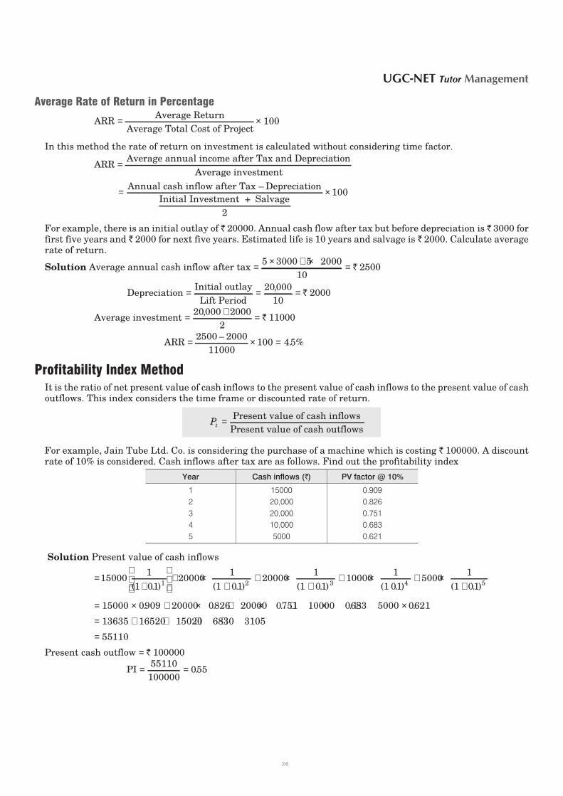
Profitability Index MethodIt is the ratio of net present value of cash inflows to the present value of cash inflows to the present value of cashoutflows. This index considers the time frame or discounted rate of return.

Pi = Present value of cash inflows

Present value of cash outflows

For example, Jain Tube Ltd. Co. is considering the purchase of a machine which is costing ` 100000. A discountrate of 10% is considered. Cash inflows after tax are as follows. Find out the profitability index

Year Cash inflows ( )̀ PV factor @ 10%

1 15000 0.909

2 20,000 0.826

3 20,000 0.751

4 10,000 0.683

5 5000 0.621

Solution Present value of cash inflows

=+

+ ×+

+ ×+

150001

1 0120000

1

1 0120000

1

11 2( . ) ( . ) ( 0110000

1

1 013 4. ) ( . )+ × + ×

+5000

1

1 01 5( . )

= × + × + × + × +15000 0909 20000 0826 20000 0751 10000 0683 5. . . . 000 0621× .

= + + + +13635 16520 15020 6830 3105

= 55110

Present cash outflow = ` 100000

PI = =55110

100000055.


26

Capital Budgeting DecisionA firm can increase its efficiency either by expanding its operations or by reducing costs. This can be done byreplacing worn out machines, renovation of plant, removal of obsolete technology, acquire fixed assets for currentand new products. Thus, budgeting decisions are of two types

(i) To expand revenues by increasing operations

(ii) To reduce costs

The first decision has higher degree of uncertainity about future revenues than the second decision which can bechecked at any stage by way of control.

National IncomeIt can be defined as the total monetary value of all final goods and services produced in a country during a periodof one year. The essential condition is that only those goods and services were included which have market value.This is national income as product flows.

National Income as Money FlowNational income can also be calculated by adding all money flows due to production activity. This is done byadding all factor costs like wages, rents, interests, profits and earnings of self-employed.

Gross Domestic Product (GDP)It is the money value of all goods and services produced within the domestic territory of a country during onefinancial year. These goods and services may be either consumer goods or capital goods. These may be producedin private sector as well as government sector. However, it does not include the value of intermediate goods andservices. The profits earned or losses incurred on account of changes in capital assets as a result of fluctuations inmarket prices, are not included in the GDP, if they are not responsible for current production of the year.

Net Domestic Product (NDP)

NDP = GDP–Depreciation on fixed capital.

Gross National Product (GNP) = GDP + Net factor income from abroad

The concept measures gross product in the light of citizenship. GDP includes income generated by foreigncitizens working in that country but does not include the income generated by the citizens of that countryworking abroad.

Net National Product (NNP) = GNP – Depreciation on capitalNDP is a geographical concept, while NNP is a national concept.

NNP at Market Price

It is the net value of final goods and services evaluated at current market price in one year after deductingdepreciation on fixed capital.

NNP at Factor Cost

It is the sum total of all incomes earned by factors of production such as wages, salaries, rents, profits, interests,taxes, incomes of self-employed, etc.

NNP at Factor Cost = NNP at market price – Indirect taxes + Subsidies = (GNP at market price –Depreciation) – Indirect taxes + Subsidies = National Income.

Private IncomeIt is the income obtained by private individuals from any source, productive or otherwise and the retainedincome of corporations.

Private Income = (NNP at factor cost) + (Transfer payments) − (Deductions)


27

Transfer payments include pensions, unemployment allowances, sickness, maternity and other social securitybenefits, gifts from abroad, windfall gains from lotteries and horse racing, and interest on public debt.

Deductions include income from government departments, surpluses of public undertakings, employee’scontributions to the provident funds and life insurance, etc.

Private income = National income + Transfer payments for non-productive individuals − social securitycontributions − Profits of government departments − surpluses of public undertakings.

Disposable IncomeIt is that actual income which can be spent on consumption by individuals and families. The whole of thepersonal income cannot be spent on consumption because a certain part of the personal income is to be paid fordirect taxes.

Disposable Income = Personal Income – Direct Taxes.

Real IncomeIt is national income expressed in terms of a general level of prices of a particular year taken as a base. Nationalincome is the value of goods and services produced as expressed in terms of money at current prices. But, it doesnot indicate the real state of the economy. It is possible that the net national product of goods and services thisyear might have been less than that of last year, but owing to an increase in prices, NNP might be higher thisyear.

To rectify such a mistake, the concept of real income has been propounded.

In order to find out the real income of a country, a year which has the general price level neither too high nor toolow is considered as a base year and the price level of that year is assumed to be 100. Now the general level ofprices of the given year for which the real NNP is to be calculated is assessed in accordance with the prices of baseyear.

Real NNP = NNP for current year × Base Year Index (100)

Current Year Index

Per Capita IncomeThe average income of the citizen of a country in a particular year is called per capita income for that year.

Per Capita Income for N th year =National Incomeof N year

Total Population in N

th

th Year

This concept enables us to know the average income and the standard of living of the people. But, it does not givea clear picture of disposable income of common man as few nations have unequal distribution of national incomewith a wide gap between poor and rich.

Methods of Measuring National IncomeIncome arises out of the process of economic activity chain.

Production generates income; Income causes spending on goods and services; Spending in turn inducesproduction. Accordingly, there are three different ways in which we can measure the size of the income.n By measuring value of output produced—Product Approachn By measuring income earned by factors—Income Approachn By measuring the size of total expenditure—Expenditure Approach

Thus, we can look at national income as a flow of goods and services, a flow of income or a flow of expenditure.

Product Approach/Output Method

Total value of final goods and services produced in a country during a year is calculated at market prices to arrive

at GDP at market price. Production from agriculture, forest, minerals from mines, goods produced by industries,contributions to production made by transport, communications, insurance companies, lawyers, doctors,teachers, hotels, entertainment, fisheries etc are collected and assessed at current market prices. Then,


Production Income Spending

28

depreciation is deducted to arrive at NDP at factor cost. Only the final goods and services are included and theintermediary goods and services, illegal productive activities are left out.

NNP = NNPFC MP + Government Subsidies – Indirect Taxes.

Income Method

Production of goods and services is an outcome of combined efforts of various factors of production like land,labour, capital and enterprise. Those factors get rewarded in form of wages, rent, interest, profit. Total incomereceived by all the factors of production in an economy during a certain period is called factor income.

These factor incomes were classified into three broad categories.

n Wage income/Labour income Income received by employees either in cash or kind.

n Capital income/Non-wage income Income paid to factors of production, in form of interest on capital, renton building, dividends, undistributed profit, interest on savings, bonus, royalties and profits of governmententerprises.

n Mixed income/Other income Earnings like direct taxes collected by government, net factor income fromabroad, value of production for self consumption.

National Income = wage income + capital income + other income.

d This approach is particularly appropriate for those activities whose output are difficult to value speciallyservice sector.

d Transfer payments such as pension, unemployment allowance, subsidies, scholarships are not included innational income.

d Wealth tax, gift tax, capital gains tax on windfall profits, sales of shares, debentures and bonds should not

be included in national income.

d Value of production for self-consumption should be included in national income.

Expenditure Method

It is based on the assumption that the income generated in an economy can be disposed either on consumption ofgoods and services or in investment. Thus, national income equals national expenditure.

n Components of final expenditure are

d Private consumption Consumption of durable and non-durable consumer goods, utility services done bypublic.

d Private investment Investment on capital goods like machines, plant setup, inventories, plots, houses.

d Government consumption Expenditure on compensation of employees, social benefits like pension,unemployment allowance, etc.

d Government investment Construction of dams, bridges, machines, transport vehicles, power plants,

etc.

d Net foreign investment All exports of merchandise and services minus all these imports in a year.

n Thus, expenditure method takes into account expenditure by houses hold, business houses and government

institutions to determine the national income.

n Household sector includes individuals, all non-government, non corporate enterprises like sole proprietorshipfirms, partnerships and non-profit institutions.

Macro-economicsn The term macro-economics was first introduced by Ragnar Frisch in 1933. Macro-economics is a study and

analysis of all the industries making an economy as a whole. It does not deal with economic problems ofindividual firms as is done in micro-economics.

n Macro-economics is the study of aggregates or average related to entire population and entire organisationsinvolved in economic activities such as total employment, national income and output, total investment, totalsavings, aggregate demand and supply, general price level, general wage level etc.


29

Scope of Macro-economicsIt covers various economic issues which concerns the nation at large scale. These are

n Theory of income and employment

n Economic fluctuations-inflation, deflation, stagflation

n International trade and economic growth.

n Causes of unemployment.

n Effect of investment on total output, total income and aggregate employment.

n Total supply of money and its impact on general price level.

n Balance of payments and foreign direct investment

n Analysis of national income.

n Growth and development of nation.

Importance of Macro-economics

The Ultimate Aim

Macro-economic studies is to formulate macro-economic policies. It helps in providing solutions to three mostpractical and critical problems any country is facing.

n Problem of economic growth To improve GDP, still developing nations like India has its GDP between7 to 8% which is still very low.

n Unemployment This problem is being faced by developing as well as developed nations, now and then.Generating sustainable employment is a major challenge for developing nations specially in countries likeIndia and China where population is very high.

n Inflation Continuous rise in the general price level of necessity goods is another problem facing nations

especially country like India, where nearly one-fourth of the population still falls below the poverty line.

Macro-economic ParadoxesProf K E Boulding pointed out three possible macro- economic paradoxes i.e., propositions which are true whenapplied to a single individual but they become false when applied to the economic system as a whole.

First Paradox-hoarding

The first paradox is that although an individual can accumulate cash balance by the process of hoarding (receiptsexceed expenditures) money, it will be his saving. But if same process of hoarding is applied to the whole nation,it could disturb the aggregate demand for goods in the market.

Second Paradox-saving and Investment

An individual saves by the process of consuming less than what he produces, thus increasing his net worth. But,this decision may not result in saving but will lead to a decline in national output and income. The aggregate ofsaving is determined by the sum of decisions to invest in capital assets.

Thirds Paradox

It is concerned with profits, wages and their distribution.

InfrastructureAccording to Albert O Hirschman, Social overhead Capital (SoC), also termed as infrastructure in commonusage, is defined as all those basic services without which primary, secondary and tertiary productive activitiescannot function.

In its wider sense, infrastructure includesn Road and transportation n Communication servicen Water and power supply n Irrigation and drainage systemsn Education n Law and order


30

Characteristics of Infrastructure1. Infrastructure is a source of external economy. It helps the organisations externally in conducting

economic activities like roads, power supply, telecom facility.

2. Infrastructure falls into the category of public utility goods. Public goods are provided by state forcollective use by citizens .

3. Infrastructure creation involves heavy expenditure which are beyond the capacity of private organisationto setup.

4. Infrastructure development is a kind of investment which creates working conditions for factories tofunction. This promotes the innovation in society.

5. Infrastructure stimulates production on a large scale by big manufacturing units and make the productaccessible to nationwide market.

Business Environmentn ‘Business’ can be defined as the planned and organised efforts of the enterprises to create and deliver value

goods and services to the consumers.

n ‘Environment’ of business consists of all those factors, internal as well as external to which business is exposedand affected.

n ‘Business Environment’ refers to the summation of all the factors which are controllable (internal) as well asuncontrollable (external) by the organisation. These factors influence the business activity on large scale. e.g.,value systems of society, government rules and regulations, monetary and fiscal policies of government,employees in the organisation, customers, suppliers, etc.

Impact of Business Environment to Enterprise

Environmental Threats

Such as changing taste and lifestyles of consumers, intense competition, foreign direct investment, decliningmarket sales etc.

New Opportunities

Exploring new market, bringing product innovation, replacing obsolete technology with latest technology,

fulfilling unmet needs which have now arised with changing standards of living.

Types of Business EnvironmentsAlthough, the term environment is generally used to refer to the external environment, which is uncontrollableby business organisations. Business firms have to adjust its internal environment to take advantages of itsstrength and opportunities and to fight with its weaknesses or threats in the business environment.

Internal Environment

The internal environment refers to all the factors within an organisation which are directly responsible for thegrowth or fall of the business unit. These are

n Value systems The value system refers to the business policies, the mission and objectives of theorganisation, practices and procedures, priorities.

n Management structure It comprises of the board of directors, top level management executives. Theirentrepreneurial skills and the extent of professionalism in approach to working affect the organisation.

n Financial capability Financial resources with the organisation, creditworthiness of the firm in the market,capital accumulation for long run functioning.

n Marketing capability Marketing and sales-force team, size of the market.

n Manpower All employees and their personal capabilities.

n Technological capabilities Availability of funds for Research and Development (R & D), technicalknow-how, latest machines, trained people.


31

External Environment

It includes all those factors which are outside the organisation, which cannot be controlled. These are againdivided into two categories.

A. Micro Environment All those factors that directly influence the business organization. These factors,though external, are very important for an organization to exist. These include

d Suppliers d Customers

d Competitors d Intermediaries

d General public

B. Macro Environment It consists of all those factors which indirectly affect the enterprises functioning.

n Economic environment All businesses are affected by national and global economic factors. The climate ofthe economy dictates how consumers, suppliers and other organisational stakeholders such as financers,creditors behave with the organisation. An economy undergoing recession will have high unemployment, lowspending power and low stakeholder confidence. Conversly, a booming economy will have high spending powerand high stakeholder confidence. Organisations have to employ strategies that protect and promote itsbusiness through economic conditions all over the world.

n Social environment It focuses its attention on forces within society such as family, friends, colleagues,neighbours and media. Social forces affect our attitudes, interests and opinion changes in the structure andlifestyle of population will affect the supply and demand of goods and services within an economy. Iforganisations do not respond to changes in society, they will loose market share and demand for their productand service.

n Technological environment Technological advances have greatly changed the manner in which businessoperate organisations use technology infrastructure such as internet, intranet or extranet to communicatewith world. Multitude of software like ERP, SAP and hardware like blackberries, bluetooth devices havegreatly increased the efficiency of business organisations. A faster exchange of information can benefitbusinesses as they are able to react quickly to changes within their operating environments.

n Political environment Political factors influence organisations in many ways. Government policies cancreate advantages and opportunities for and organisations conversely, they can place obligations and duties onorganizations. Political factors include

d Legislation such as minimum wage, anti-discrimination laws.

d Voluntary codes and practices d Market regulations

d Trade agreements, tarriffs d Tax levies

d Type of government regime


32

Quick RecapA. Great Economists■ Adam Smith Father of Economics

■ Ragnar Frisch introduced the term

Micro and Macro Economics

■ Marginal utility analysis Alfred Marshall

■ Law of Diminishing Marginal Utility Heinrich Gossen

■ Demand paradox for inferior goods Sir Robert Giffen

■ Consumer's Surplus Marshall

■ ‘‘Value and Capital’’ book JR Hicks

■ Theory of circular causation Ragnar Nurkse

■ Indifference curve analysis Hicks and Allen

■ Revealed Preference Theory Samuelson

■ Substitution effect Hicks Allen

■ Scientific touch to Indifference curve analyses

FY Edgeworth

■ Principles of Economics Alfred Marshall

■ Diamond Water Paradox Adam Smith

■ Asian Drama Gunnar Myrdal

■ Language of Economics JK Galbraith

■ Degrees of Price Discrimination AC Pigou

■ Kinked demand curve hypothesis Paul M Sweezy

■ Demonstration effect Thorstein Veblen

■ Product exhaustion theorem Clark Wicksteed

■ Demand schedule at various prices Catherin

■ Monopsony concept Mrs J Robinson

■ Infant industry Argument Freidrich List

■ Social-Accounting concept JR Hicks

■ Zero based budgeting Jimmy Carter

B. Basic Concepts of Managerial Economics■ Law of demand establishes qualitative or directional relationship

between demand and price.

■ Demand curve for a commodity is drawn on the assumption that thetaste, income and price of other goods remain constant. Thisassumption is termed as ‘‘Cetirus Paribus’’.

■ Perfectly elastic demand — Ed = ∞ (infinite)

■ Perfectly inelastic demand — Ed = 0 (zero)

■ Unitary elastic demand — Ed =1

■ Relatively inelastic demand Ed <1

■ Elastic demand , Ed>1

■ Exception to the law of demand— demonstration effect goods,Giffen's inferior goods, future scarcity of goods, ignorance ofconsumer.

■ Demand curve moves downward due to law of diminishing MU andincome effect.

■ Elasticity of demand measures the responsiveness of demand tochange in prices.

■ Income elasticity e i =∆ ∆Q

Q

y

y÷ where y= income Q = Quantity

demanded

■ Arc elasticity ea =Q Q

Q Q

P P

P P1 2

1 2

1 2

1 2

−+

÷ −+

■ Movement along demand curve due to change in price causesexpansion or contraction of demand.

■ Shift in demand curve due to change in factors other than the pricelike income, taste, price of substitutes or complementary goodscauses increase or decrease of demand.

■ Production possibility curve is concave to origin because ofincreasing MRT (Marginal Rate of Transformation) between X and Y.

■ In case of Giffen's goods, price effect is negative with increase inprice, demand decreases.

■ If demand curve is a rectangular hyperbola, elasticity is one.

■ Cross elasticity of demand for substitutes is positive.

■ Cross elasticity of demand for complementary goods is negative.

■ When average revenue becomes constant, AR = MR

■ The falling part of total utility curve shows negative marginal utility.

■ Total utility is maximum when MU = 0.

■ At the shut-down point, a firm is having all total losses equal totalfixed cost, total revenue equal total variable cost, price is equal toaverage variable cost.

■ The emphasis of managerial economics is on normative theorywhich is more of empirical study.

■ Cobb Douglas production function is linear homogeneous

production function of first degree presented as P K L C= 1 4 3 4 1 4/ / / .

■ Condition of perfect competition firm’s equilibrium – MC = MR, MR= price, slope of MC should be greater than slope of MR. Long runequilibrium of the firm is established at minimum point of LAC.

■ Long-run Average Cost curve (LAC) takes L-shape because of tworeasons-Technological progress and learning by-doing.

■ Under price discrimination, market having less elasticity of demandcan be charged higher price.

■ Economics of scale implies reduction, in unit cost of production.

■ Law of equi-marginal utility –MUx

Px

PUy

PyMUm= =

■ In case of unitary price elasticity of demand, total expenditureremains constant i.e., has no price effect.

■ Diamond water paradox establishes the fact that marginal utility canbe low but total utility will be high for necessary goods like water.

■ GNP = GDP + Net faction income from abroad.

■ NNP = GNP – depreciation

■ Monopoly – single seller

■ Bilateral monopoly-single seller, single buyer

■ Monopsony—Single buyer, many sellers

■ Duopoly—Two sellers, many buyers.

■ Learner’s Degree of Monopoly Power = − =P

p e

MC 1

■ SAC is U shaped and more pronounced

■ LAC is U shaped and less pronounced -envelope of SACs

■ Stage of PLC - Introduction, growth, maturity, saturation, decline.

■ BEP (units) =−TFC

MCP

33

■ Gossen’s first Law– Law of diminishing marginal utility.

■ Gossen’s second law–Law of equimarginal utility

■ Indifference curve is based on ordinal utility just as marginal utilityanalysis is based on cardinal utility.

■ L-Shaped indifference curve indicates perfect complementarygoods with zero MRxy .

■ Consumer’s indifference curve for perfect substitutes is downwardsloping straight line.

■ MRSxy is decreasing–IC curve is convex to origin.

■ MRSxy is zero – L- shaped IC curve (complementary goods)

■ MRSxy is increasing – IC curve is concave to origin.

■ MRSxy is constant–IC is downwards sloping straight line(substitutes)

■ MRSxy = − ∆∆

y

x

■ Smoothness and continuity of indifference curves means that goodsin question are assumed to be perfectly divisible.

■ Budget line is the various combinations of the two commodities thata consumer can purchase at a fixed income level.

■ A consumer reaches equilibrium when MU= P

■ eAR

AR MR=

–or MR =

ARe

11

–

■ Revealed Preference Theory of Samuelson is based on strongordering of observed consumer behaviour.


34

Factolight(Based on Previous Years’ Paper)

1. Demand curve under monopolistic competition isdownward sloping and flat. [Jun 2005]

2. If two commodities are complementary, then a rise in

price of one commodity will induce a backward shift in

demand for the other commodity. [Jun 2005]

3. If the demand curve is rectangular hyperbola, the

elasticity is unity. [Jun 2005]

4. Income is a flow variable where as product, capital

formation and wealth is a static variable. [Jun 2005]

5. “Supply creates its own demand” is known as Says

Law. [Jun 2005]

6. In the law of variable proportions, phase two indicates

diminishing returns. [Dec 2005]

7. The demand curve facing the pure monopolist is

negatively sloped. [Dec 2005]

8. Total consumer expenditure on a good falls as its price

falls; this indicates that its price elasticity is less than

one. [Dec 2005]

9. National income is NNP at factor cost. [Dec 2005]

10. A firm produces output using labour and capital. Ifprices of both inputs double, then the total minimumcost of producing any given level of output is doubledprovided the firm has constant returns to scaletechnology. [Jun 2006]

11. In the long run a firm under perfectly competitivemarket earns only normal profit. [Jun 2006]

12. National income at current prices is equal to NNP atfactor cost. [Jun 2006]

13. A monopolist always charges a price which is greater

than marginal cost. [Jun 2006]

14. The Kinky demand curve hypothesis predicts sticky

prices in the market. [Jun 2006]

15. Price elasticity of demand for luxury goods will be

infinitely elastic. [Dec 2006]

16. In the short run, profit maximizing firm produces

additional units of production, as long as marginal

revenue exceeds marginal cost. [Dec 2006]

17. In the typical demand schedule, quantity demanded

varies inversely with price. [Dec 2006]

18. Shut down point is that point where price is equal to

variable cost. [Dec 2006]

19. Bank rate, CRR and trading of shares in open market

are monitory policies but taxation is a fiscal policy.

[Dec 2006]

20. The assumption that economic conflict between the

organization leads to innovativeness and the new

product development, technological advancement and

better services at lower prices, refers to Cost Reduction

strategy. [Dec 2006]

21. ISO Cost Line is also called as production line.

[Jun 2007]

22. Quadratic cost function is written as TC = a + bQ+cQ2

[Jun 2007]

23. Transfer pricing is referred to as price charged under

intra firm transfer of product. [Jun 2007]

24. Margin of safety is above the break even point.

[Jun 2007]

25. Profit is maximized when MC = MR. [Jun 2007]

26. The shape of short run average cost curve is U shaped.

` [Jun 2007]

27. Bax-Jenkin is one of the important methods used in

trend projection of sales forecast. [Dec 2007]

28. The Cobb Douglas production function has the

equation P = AK(a)L(1-a). [Dec 2007]

29. Skimming price for a new product is high initial price.

[Dec 2007]

30. Under monopoly market structure, the degree of

freedom in pricing decision is quite good. [Dec 2007]

31. Capital budgeting decisions are generally irreversible.

[Dec 2007]

32. Intervention of the Government is not the

pre-requisite of a perfect market. [Dec 2007]

33. The demand curve of a monopolistically competitive

firm is highly though not perfectly elastic. [Jun 2008]

34. A decision maker has to remember the proverb, “a bird

in hand is worth two in bush”, while he examines

Opportunity Cost principle. [Jun 2008]

35. Market with one buyer and one seller is called bilateralmonopoly. [Jun 2008]

36. Cardinal measure of utility is required in UtilityTheory. [Jun 2008]

37. In case of Giffen goods, price effect is positive.

[Jun 2008]

38. The term opportunity cost refers to cost of one productin terms of production of others sacrificed. [Dec 2008]

39. Consumer’s willingness to pay minus (–) actualpayment is called Consumer’s Surplus. [Dec 2008]

40. The pay-back period refers to the number of years aproject takes to recover its investment cost. [Dec 2008]

35

41. In the case of Veblen goods, demand curve will slopeupwards. [Dec 2008]

42. Monopolist can decide either price or quantity but not

both. [Dec 2008]

44. Price elasticity of demand is best described as the rate

of response of demand to a change in price. [Jun 2009]

45. Giffen goods are those goods for which demand

increases as price increases. [Jun 2009]

46. The situation where market consists of only two buyers is

known as Duopsony. [Jun 2009]

47. Short run cost curves are influenced by Laws of

variable proportion. [Jun 2009]

48. The term opportunity cost refers to cost of one product

in terms of production of others foregone. [Jun 2009]

49. The elasticity of demand indicates the rate of response

of demand to a change in price. [Dec 2009]

50. A rightward shift in supply curve indicates an increase

in supply. [Dec 2009]

51. The condition of equilibrium for the monopolist is

MR = MC. [Dec 2009]

52. Price control leads to rationing and black marketing

under perfect competition. [Dec 2009]

53. If both supply and demand increase by the same

proportion, price remains constant. [Dec 2009]

54. During last five years, per capita income of India isincreasing, that means national income growth ofIndia is more than the population growth. [Jun 2010]

55. In the short-run firm considers the minimum of itsaverage variable cost curve as shut down point.

[Jun 2010]

56. The positive cross elasticity of demand between twoproducts means two products are substitutes.

[Jun 2010]

57. A monopolist always operates in the elastic segment ofits demand curve. [Jun 2010]

58. The price elasticity of demand for any product in thelong-run is more than its short run value. [Jun 2010]

59. Under perfect competition in the long run, all firms earnnormal profits. [Dec 2010]

60. National Income at market prices is equal to NNP atFactor cost. [Dec 2010]

61. If there is a single buyer, it is called Monopsony.

[Dec 2010]

62. Time value of money is considered for NPV, IRR butnot for Pay-back method. [Dec 2010]

63. A firm is having increasing returns to scale means it ishaving decreasing costs. [Dec 2010]


36

managerial economics - images-na.ssl-images · pdf filescope of managerial economics demand...

Documents