managerial economics - unit 1: demand theory · objectives role of managers ... i consumer tastes f...
TRANSCRIPT
Managerial EconomicsUnit 1: Demand Theory
Rudolf Winter-Ebmer
Johannes Kepler University Linz
Summer Term 2018
Winter-Ebmer, Managerial Economics: Unit 1 - Demand Theory 1 / 55
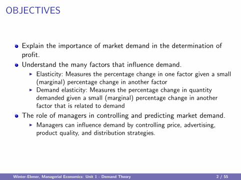
OBJECTIVES
Explain the importance of market demand in the determination ofprofit.
Understand the many factors that influence demand.I Elasticity: Measures the percentage change in one factor given a small
(marginal) percentage change in another factorI Demand elasticity: Measures the percentage change in quantity
demanded given a small (marginal) percentage change in anotherfactor that is related to demand
The role of managers in controlling and predicting market demand.I Managers can influence demand by controlling price, advertising,
product quality, and distribution strategies.
Winter-Ebmer, Managerial Economics: Unit 1 - Demand Theory 2 / 55
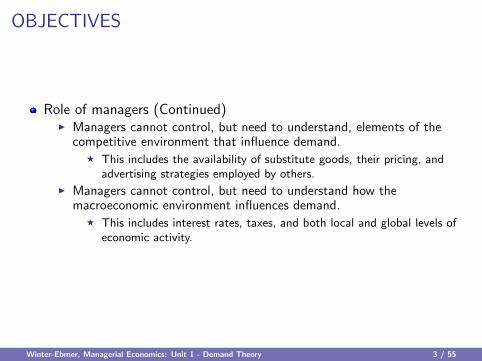
OBJECTIVES
Role of managers (Continued)I Managers cannot control, but need to understand, elements of the
competitive environment that influence demand.F This includes the availability of substitute goods, their pricing, and
advertising strategies employed by others.
I Managers cannot control, but need to understand how themacroeconomic environment influences demand.
F This includes interest rates, taxes, and both local and global levels ofeconomic activity.
Winter-Ebmer, Managerial Economics: Unit 1 - Demand Theory 3 / 55

How to use this chapter
For most students almost all in this chapter should be well-known.Later on I will assume that students, indeed, know these concepts.
I will be very quick and present only a small part.
Students should read the chapter carefully, if they see problems.
Winter-Ebmer, Managerial Economics: Unit 1 - Demand Theory 4 / 55

Winter-Ebmer, Managerial Economics: Unit 1 - Demand Theory 5 / 55
Winter-Ebmer, Managerial Economics: Unit 1 - Demand Theory 6 / 55
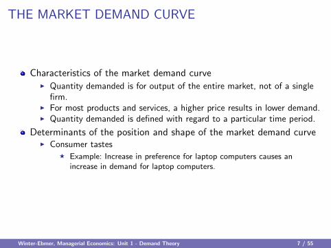
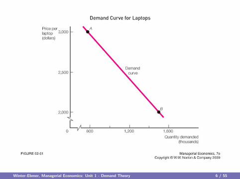
THE MARKET DEMAND CURVE
Characteristics of the market demand curveI Quantity demanded is for output of the entire market, not of a single
firm.I For most products and services, a higher price results in lower demand.I Quantity demanded is defined with regard to a particular time period.
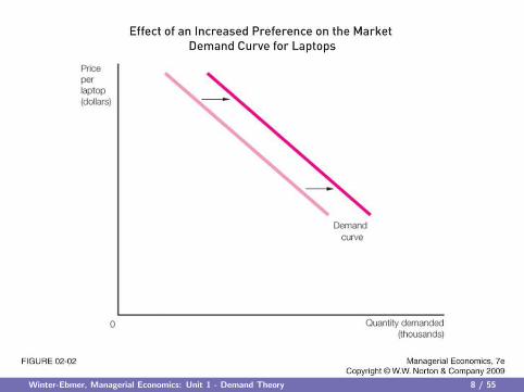
Determinants of the position and shape of the market demand curveI Consumer tastes
F Example: Increase in preference for laptop computers causes anincrease in demand for laptop computers.
Winter-Ebmer, Managerial Economics: Unit 1 - Demand Theory 7 / 55
Winter-Ebmer, Managerial Economics: Unit 1 - Demand Theory 8 / 55
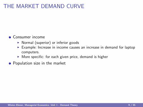
THE MARKET DEMAND CURVE
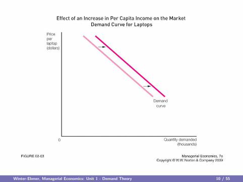
Consumer incomeI Normal (superior) or inferior goodsI Example: Increase in income causes an increase in demand for laptop
computers.I More specific: for each given price, demand is higher
Population size in the market
Winter-Ebmer, Managerial Economics: Unit 1 - Demand Theory 9 / 55
Winter-Ebmer, Managerial Economics: Unit 1 - Demand Theory 10 / 55
INDUSTRY AND FIRM DEMAND FUNCTIONS
Market demand function: The relationship between the quantitydemanded and the various factors that influence this quantity
I Quantity of X (Q) = f(factors)I Factors include
F price of XF incomes of consumersF tastes of consumersF prices of other goodsF populationF advertising expenditures
Winter-Ebmer, Managerial Economics: Unit 1 - Demand Theory 11 / 55
INDUSTRY AND FIRM DEMAND FUNCTIONS
Example: Q = b1P + b2I + b3S + b4AI Assumes that population is constant and that the demand function is
linearI P = price of laptopsI I = per capita disposable incomeI S = average price of softwareI A = amount spent on advertisingI b1, b2, b3 and b4 are parameters that are estimated using statistical
methods
Winter-Ebmer, Managerial Economics: Unit 1 - Demand Theory 12 / 55
INDUSTRY AND FIRM DEMAND FUNCTIONS
Interpretation of Parameters:I Q = b1P + b2I + b3S + b4AI E.g. b1: if Price changes by one unit, quantity demanded changes by b1
units under the condition that all other variables (i.e. price of Software)are held constant
I Example:F Q = −700P + 200I − 500S + 0.01A
Winter-Ebmer, Managerial Economics: Unit 1 - Demand Theory 13 / 55
The firm’s demand curve
Negative slope with regard to priceI Slope may not be the same as that of the market demand curve.
Represents a portion of market demandI Market shareI Responds to same market and macroeconomic factors as the market
demand curve
Directly related to the prices of substitute goods provided bycompetitors
I Increase in competitor’s price will cause a increase in a firm’s demand.
Winter-Ebmer, Managerial Economics: Unit 1 - Demand Theory 14 / 55
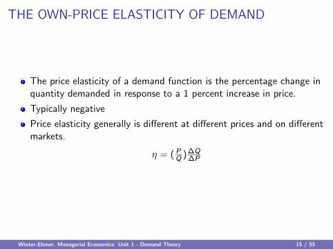
THE OWN-PRICE ELASTICITY OF DEMAND
The price elasticity of a demand function is the percentage change inquantity demanded in response to a 1 percent increase in price.
Typically negative
Price elasticity generally is different at different prices and on differentmarkets.
η = (PQ ) ∆Q
∆P
Winter-Ebmer, Managerial Economics: Unit 1 - Demand Theory 15 / 55
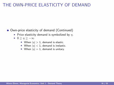
THE OWN-PRICE ELASTICITY OF DEMAND
Own-price elasticity of demand (Continued)I Price elasticity demand is symbolized by η.I 0 ≥ η ≥ −∞
F When |η| > 1, demand is elastic.F When |η| < 1, demand is inelastic.F When |η| = 1, demand is unitary.
Winter-Ebmer, Managerial Economics: Unit 1 - Demand Theory 16 / 55
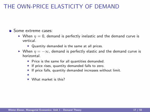
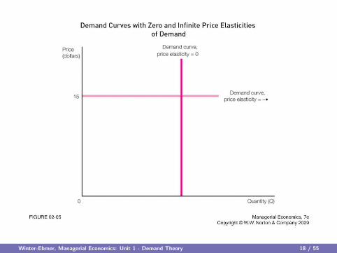
THE OWN-PRICE ELASTICITY OF DEMAND
Some extreme cases:I When η = 0, demand is perfectly inelastic and the demand curve is
vertical.F Quantity demanded is the same at all prices.
I When η = −∞, demand is perfectly elastic and the demand curve ishorizontal.
F Price is the same for all quantities demanded.F If price rises, quantity demanded falls to zero.F If price falls, quantity demanded increases without limit.F
F What market is this?
Winter-Ebmer, Managerial Economics: Unit 1 - Demand Theory 17 / 55
Winter-Ebmer, Managerial Economics: Unit 1 - Demand Theory 18 / 55
Looks simple, but. . .
this is the most important insight of this lecture:I Typically demand curve is downward slopingI That means, we are in a market, which is not fully competitiveI If this were not the case (i.e perfect competition), everything would be
boring:F Marketing, pricing, . . . would make no sense
Winter-Ebmer, Managerial Economics: Unit 1 - Demand Theory 19 / 55

THE OWN-PRICE ELASTICITY OF DEMAND
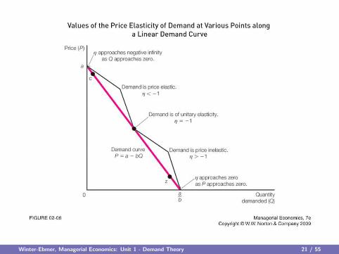
Example: linear demand curvesI The slope of a linear demand curve is constant.I price elasticity will differ depending on price.
F At the midpoint of a linear demand curve, η = −1, with η approachingzero as price approaches the vertical intercept.
F At prices above the midpoint, demand is elastic, with η approachingnegative infinity as price approaches zero.
F At prices below the midpoint, demand is inelastic.
Winter-Ebmer, Managerial Economics: Unit 1 - Demand Theory 20 / 55
Winter-Ebmer, Managerial Economics: Unit 1 - Demand Theory 21 / 55
Knowing the elasticity
Every manager must know elasticity of demand for main products
How can we do that?
Very easy to calculate
Winter-Ebmer, Managerial Economics: Unit 1 - Demand Theory 22 / 55
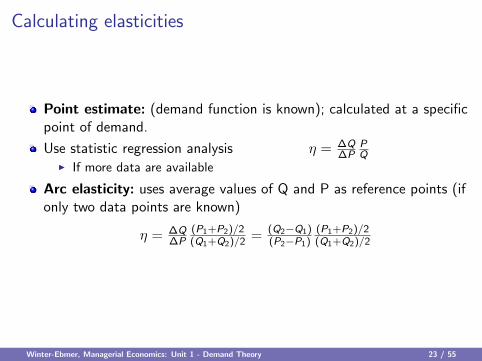
Calculating elasticities
Point estimate: (demand function is known); calculated at a specificpoint of demand.
Use statistic regression analysis η = ∆Q∆P
PQ
I If more data are available
Arc elasticity: uses average values of Q and P as reference points (ifonly two data points are known)
η = ∆Q∆P
(P1+P2)/2(Q1+Q2)/2 = (Q2−Q1)
(P2−P1)(P1+P2)/2(Q1+Q2)/2
Winter-Ebmer, Managerial Economics: Unit 1 - Demand Theory 23 / 55
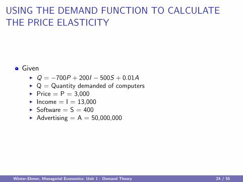
USING THE DEMAND FUNCTION TO CALCULATETHE PRICE ELASTICITY
GivenI Q = −700P + 200I − 500S + 0.01AI Q = Quantity demanded of computersI Price = P = 3,000I Income = I = 13,000I Software = S = 400I Advertising = A = 50,000,000
Winter-Ebmer, Managerial Economics: Unit 1 - Demand Theory 24 / 55
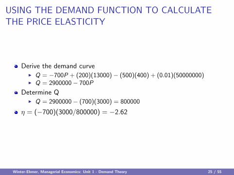
USING THE DEMAND FUNCTION TO CALCULATETHE PRICE ELASTICITY
Derive the demand curveI Q = −700P + (200)(13000)− (500)(400) + (0.01)(50000000)I Q = 2900000− 700P
Determine QI Q = 2900000− (700)(3000) = 800000
η = (−700)(3000/800000) = −2.62
Winter-Ebmer, Managerial Economics: Unit 1 - Demand Theory 25 / 55
If you increase the price, how will your revenue react?
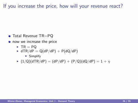
Total Revenue TR=PQ
now we increase the priceI TR = PQI dTR/dP = Q(dP/dP) + P(dQ/dP)
F Simplify
I (1/Q)(dTR/dP) = (dP/dP) + (P/Q)(dQ/dP) = 1 + η
Winter-Ebmer, Managerial Economics: Unit 1 - Demand Theory 26 / 55
If you increase the price, how will your revenue react?
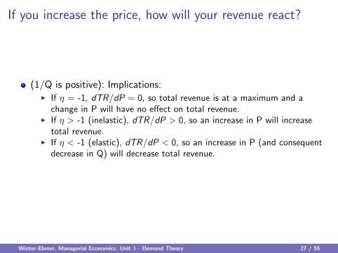
(1/Q is positive): Implications:I If η = -1, dTR/dP = 0, so total revenue is at a maximum and a
change in P will have no effect on total revenue.I If η > -1 (inelastic), dTR/dP > 0, so an increase in P will increase
total revenue.I If η < -1 (elastic), dTR/dP < 0, so an increase in P (and consequent
decrease in Q) will decrease total revenue.
Winter-Ebmer, Managerial Economics: Unit 1 - Demand Theory 27 / 55
Recap: What are the important issues?
Markets are not perfect; therefore pricing and advertising is important
Know the demand curve
Price elasticity: do not set price, where demand is inelastic
Optimal pricing rule
Winter-Ebmer, Managerial Economics: Unit 1 - Demand Theory 28 / 55

Example: FUNDING PUBLIC TRANSIT
GivenI Price (fare) elasticity of demand for public transit in the United States
is about -0.3.I Many public transit systems lose money.I Public transit systems are funded by federal, state, and local
governments, all of which have budget issues.
Winter-Ebmer, Managerial Economics: Unit 1 - Demand Theory 29 / 55
FUNDING PUBLIC TRANSIT
Which transit systems have the most difficult time getting publicfunding?
I Revenue from sales will increase if fares are increased, because demandis inelastic.
I Costs will likely decrease if fares are increased, because quantitydemanded (ridership) will fall.
I Managers of public transit will therefore increase fares if they do notreceive enough public funds to balance their budgets.
I Public funding seems necessary to prevent price hikes
Winter-Ebmer, Managerial Economics: Unit 1 - Demand Theory 30 / 55
DETERMINANTS OF OWN-PRICE ELASTICITY OFDEMAND
Number and similarity of available substitutes
Product price relative to a consumer’s total budget
Time period available for adjustment to a price changeI Ex: Cell phone contracts, gasoline prices
Winter-Ebmer, Managerial Economics: Unit 1 - Demand Theory 31 / 55
Winter-Ebmer, Managerial Economics: Unit 1 - Demand Theory 32 / 55
WHY ARE THERE MARKETS WITH LOW ELASTICITYOF DEMAND?
Elasticity is calculated for the market (as a whole)
What is elasticity if the firm changes the price alone?
Competitive situation in the industry has to be taken into account
It seems that in markets with relatively low elasticities are marketswhere unilateral price hikes are difficult
Firm-specific price elasticity of demand is the one which is importantfor price setting!!
Winter-Ebmer, Managerial Economics: Unit 1 - Demand Theory 33 / 55
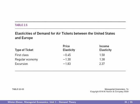
THE STRATEGIC USE OF THE PRICE ELASTICITY OFDEMAND
Example: Strategic pricing of first class (η= -0.45), regular economy(η= -1.30) and excursion (η= -1.83) airline tickets between theUnited States and Europe
I First class prices should be relatively high because demand is inelastic.I Regular economy and excursion prices should be relatively low because
demand is elastic.
Winter-Ebmer, Managerial Economics: Unit 1 - Demand Theory 34 / 55
Winter-Ebmer, Managerial Economics: Unit 1 - Demand Theory 35 / 55
THE STRATEGIC USE OF THE PRICE ELASTICITY OFDEMAND
Example: Using differentiation strategies to change the price elasticityof demand for a product
I Differentiation strategies convince consumers that a product is unique,and therefore has fewer substitutes.
I Role of advertising
Winter-Ebmer, Managerial Economics: Unit 1 - Demand Theory 36 / 55
THE STRATEGIC USE OF THE PRICE ELASTICITY OFDEMAND
Example (Continued)I If consumers perceive that a product has fewer substitutes, then their
price elasticity of demand for the product will decrease (become lesselastic) in absolute value.
I Differentiation strategies do not require actual differences in products,only a perceived difference.
Winter-Ebmer, Managerial Economics: Unit 1 - Demand Theory 37 / 55
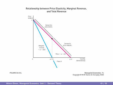
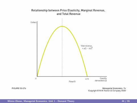
TOTAL REVENUE, MARGINAL REVENUE, AND PRICEELASTICITY
A firm’s total revenue (TR) is equal to the total amount of moneyconsumers spend on the product in a given time period.
I Linear demand curve: P = a− bQI Corresponding total revenue:
F TR = PQ = aQ − bQ2
Winter-Ebmer, Managerial Economics: Unit 1 - Demand Theory 38 / 55
TOTAL REVENUE, MARGINAL REVENUE, AND PRICEELASTICITY
Marginal revenue: The incremental revenue earned from selling thenth unit of output.
I MR = ∆TR/∆Q = ∆(aQ − bQ2)/∆Q = a− 2bQF η = (−1/b)[(a− bQ)/Q]F If Q = a/2b, then η = -1F If Q > a/2b, then η is inelasticF If Q < a/2b, then η is elastic
Winter-Ebmer, Managerial Economics: Unit 1 - Demand Theory 39 / 55
TOTAL REVENUE, MARGINAL REVENUE, AND PRICEELASTICITY
Marginal revenue (Continued)I MR = ∆TR/∆Q = ∆(PQ)/∆Q =
= P(∆Q/∆Q) + Q(∆P/∆Q) == P[1 + (Q/P)(∆P/∆Q)]
F so MR = P(1 + 1/η)
If product is price elastic (η < −1), marginal revenue must be positive
Example: what is MR if price is AC10 and price elasticity is -2?10(1+1/(-2)) = AC5.
What if product is very price elastic (η = −∞)?
Winter-Ebmer, Managerial Economics: Unit 1 - Demand Theory 40 / 55
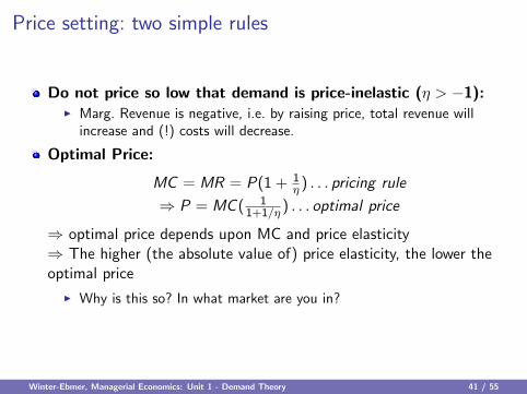
Price setting: two simple rules
Do not price so low that demand is price-inelastic (η > −1):I Marg. Revenue is negative, i.e. by raising price, total revenue will
increase and (!) costs will decrease.
Optimal Price:
MC = MR = P(1 + 1η ) . . . pricing rule
⇒ P = MC ( 11+1/η ) . . . optimal price
⇒ optimal price depends upon MC and price elasticity⇒ The higher (the absolute value of) price elasticity, the lower theoptimal price
I Why is this so? In what market are you in?
Winter-Ebmer, Managerial Economics: Unit 1 - Demand Theory 41 / 55
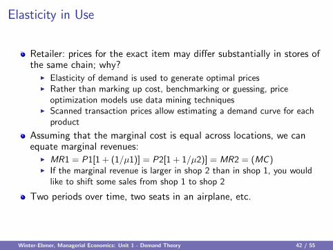
Elasticity in Use
Retailer: prices for the exact item may differ substantially in stores ofthe same chain; why?
I Elasticity of demand is used to generate optimal pricesI Rather than marking up cost, benchmarking or guessing, price
optimization models use data mining techniquesI Scanned transaction prices allow estimating a demand curve for each
product
Assuming that the marginal cost is equal across locations, we canequate marginal revenues:
I MR1 = P1[1 + (1/µ1)] = P2[1 + 1/µ2)] = MR2 = (MC )I If the marginal revenue is larger in shop 2 than in shop 1, you would
like to shift some sales from shop 1 to shop 2
Two periods over time, two seats in an airplane, etc.
Winter-Ebmer, Managerial Economics: Unit 1 - Demand Theory 42 / 55
Winter-Ebmer, Managerial Economics: Unit 1 - Demand Theory 43 / 55
Winter-Ebmer, Managerial Economics: Unit 1 - Demand Theory 44 / 55
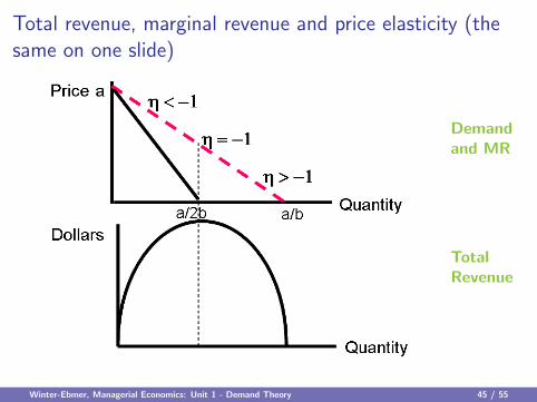
Total revenue, marginal revenue and price elasticity (thesame on one slide)
Demandand MR
TotalRevenue
Winter-Ebmer, Managerial Economics: Unit 1 - Demand Theory 45 / 55
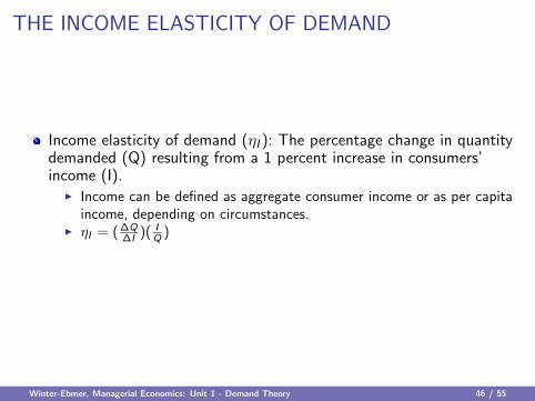
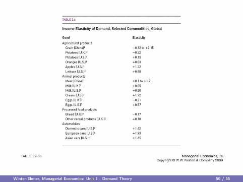
THE INCOME ELASTICITY OF DEMAND
Income elasticity of demand (ηI ): The percentage change in quantitydemanded (Q) resulting from a 1 percent increase in consumers’income (I).
I Income can be defined as aggregate consumer income or as per capitaincome, depending on circumstances.
I ηI = ( ∆Q∆I )( I
Q )
Winter-Ebmer, Managerial Economics: Unit 1 - Demand Theory 46 / 55
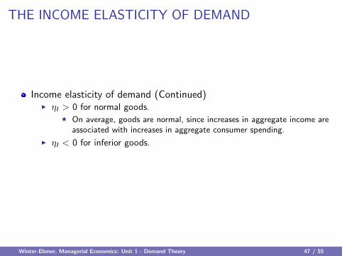
THE INCOME ELASTICITY OF DEMAND
Income elasticity of demand (Continued)I ηI > 0 for normal goods.
F On average, goods are normal, since increases in aggregate income areassociated with increases in aggregate consumer spending.
I ηI < 0 for inferior goods.
Winter-Ebmer, Managerial Economics: Unit 1 - Demand Theory 47 / 55
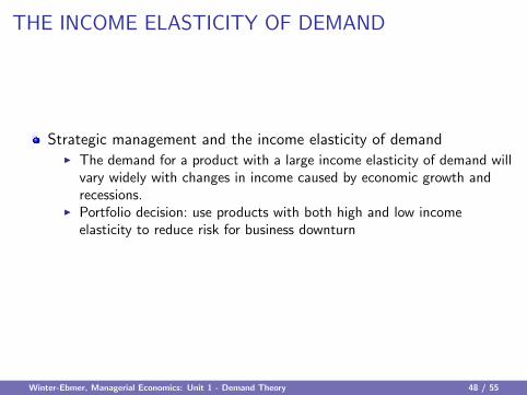
THE INCOME ELASTICITY OF DEMAND
Strategic management and the income elasticity of demandI The demand for a product with a large income elasticity of demand will
vary widely with changes in income caused by economic growth andrecessions.
I Portfolio decision: use products with both high and low incomeelasticity to reduce risk for business downturn
Winter-Ebmer, Managerial Economics: Unit 1 - Demand Theory 48 / 55
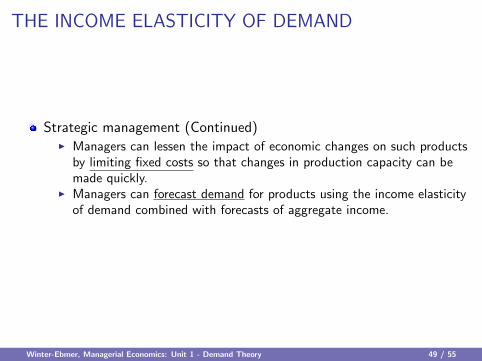
THE INCOME ELASTICITY OF DEMAND
Strategic management (Continued)I Managers can lessen the impact of economic changes on such products
by limiting fixed costs so that changes in production capacity can bemade quickly.
I Managers can forecast demand for products using the income elasticityof demand combined with forecasts of aggregate income.
Winter-Ebmer, Managerial Economics: Unit 1 - Demand Theory 49 / 55
Winter-Ebmer, Managerial Economics: Unit 1 - Demand Theory 50 / 55
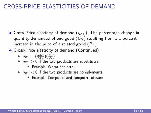
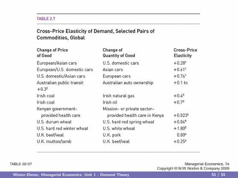
CROSS-PRICE ELASTICITIES OF DEMAND
Cross-Price elasticity of demand (ηXY ): The percentage change inquantity demanded of one good (QX ) resulting from a 1 percentincrease in the price of a related good (PY )
Cross-Price elasticity of demand (Continued)I ηXY = ( ∆QX
∆PY)( PY
QX)
I ηXY > 0 if the two products are substitutes.F Example: Wheat and corn
I ηXY < 0 if the two products are complements.F Example: Computers and computer software
Winter-Ebmer, Managerial Economics: Unit 1 - Demand Theory 51 / 55
CROSS-PRICE ELASTICITIES OF DEMAND
Strategic managementI Managers can use information about the cross-price elasticity of
demand to predict the effect of competitors’ pricing strategies on thedemand for their product.
I Antitrust authorities use the cross-price elasticity of demand todetermine the likely effect of mergers on the degree of competition inan industry.
Winter-Ebmer, Managerial Economics: Unit 1 - Demand Theory 52 / 55
CROSS-PRICE ELASTICITIES OF DEMAND
Strategic managementI Antitrust authorities (Continued)
F A high cross-price elasticity, indicating that two goods are strongsubstitutes, suggests that a merger would significantly reducecompetition in the industry.
F A low cross-price elasticity, indicating that two goods are strongcomplements, suggests that a merger might give the merged firmexcessive control over the supply chain.
Winter-Ebmer, Managerial Economics: Unit 1 - Demand Theory 53 / 55
THE ADVERTISING ELASTICITY OF DEMAND
Advertising elasticity of demand (ηA): The percentage change inquantity demanded (Q) resulting from a 1 percent increase inadvertising expenditure (A)
I ηA = ( ∆Q∆A )( A
Q )I Example Calculation
F Given: Q = 500− 0.5P + 0.01I + 0.82A and A/Q = 2F ηA = 0.82(2) = 1.64
Winter-Ebmer, Managerial Economics: Unit 1 - Demand Theory 54 / 55
Winter-Ebmer, Managerial Economics: Unit 1 - Demand Theory 55 / 55