managerial economy 13.indd - managerial economics
TRANSCRIPT


Redakcja Wydawnictw AGH al. Mickiewicza 30, 30-059 Kraków tel. 12 617 32 28, tel./faks 12 636 40 38e-mail: [email protected]; http://www.wydawnictwa.agh.edu.pl
AGH Press Editor-in-Chief: Jan Sas
Managerial Economics Periodical Editorial Board
Editor-in-Chief:Henryk Gurgul (AGH University of Science and Technology in Krakow, Poland)
Associate Editors:Mariusz Kudełko (AGH University of Science and Technology in Krakow, Poland) economics, managementStefan Schleicher (Karl-Franzens-Universität Graz, Austria) quantitative methods in economics and management
Managing Editor:Joanna Duda (AGH University of Science and Technology in Krakow, Poland)
Technical Editor:Łukasz Lach (AGH University of Science and Technology in Krakow, Poland)
Editorial Board:Gerrit Brösel (Fern Universität Hagen, Germany)Piotr Górski (AGH University of Science and Technology in Krakow, Poland) Ingo Klein (Universität Erlangen-Nürnberg, Germany) Marianna Księżyk (Andrzej Frycz Modrzewski Krakow University, Poland) Manfred Jürgen Matschke (Universität Greifswald, Germany) Xenia Matschke (Universität Trier, Germany)Roland Mestel (FH Joanneum Graz, Austria)
Articles published in the semi-annual Managerial Economics have been peer reviewed by re-viewers appointed by the Editorial Board. The procedure for reviewing articles is described at the following web address: http://www.managerial.zarz.agh.edu.pl
Reviewers: Gerrit Brösel, Heinz Eckart Klingelhöfer, Michael Olbrich, Stefan Palan, Karl Farmer, Manfred Jürgen Matschke, Christoph Mitterer, Jerzy Mika, Janusz Teczke, Czesław Mesjasz
Language Editor: Norman L. Butler
Statistical Editor: Anna Barańska
Editorial support: Magdalena Grzech
Cover and title page design: Zofia Łucka
DOI: http://dx.doi.org/10.7494/manage
© Wydawnictwa AGH, Kraków 2013, ISSN 1898-1143
Nakład 80 egz. The printed version of the journal is the primery one.

5
SpiS treści
Joanna Duda
The Role of Bank Credits in Investment Financing of the Small and Medium-sized Enterprise Sector in Poland ...................................................... 7
Henryk Gurgul, Roland Mestel, Robert Syrek
The Testing of Causal Stock Returns-Trading Volume Dependencies with the Aid of Copulas ........................................................................................... 21
Henryk Gurgul, Artur Machno, Roland Mestel
Modeling of Returns and Trading Volume by Regime Switching Copulas ..... 45
Henryk Gurgul, Marcin Suder
Modeling of Withdrawals from Selected ATMs of the “Euronet” Network ..... 65
Katarzyna Liczmańska, Agnieszka M. Wiśniewska
A Strong Brand as a Determinant of Purchase the Case of Sectors, where Advertising in Mass Media Is Banned – on the Example of the Polish Spirits Sector .................................................................................. 83
Paweł Zając
The New Approach to Estimation of the Hazard Function in Business Demography on Example of Data from New Zealand .................................... 99
Summaries ....................................................................................................... 111
Streszczenia ...................................................................................................... 115
Instruction for authors ..................................................................................... 119
Informacje dla autorów artykułów .................................................................. 121

7
Managerial Economics2013, No. 13, pp. 7–20
http://dx.doi.org/10.7494/manage.2013.13.7
Joanna Duda*
the role of Bank credits in investment Financing of the Small and Medium‑sized enterprise Sector in poland
1. introduction
Small and medium-sized enterprises have considerable impact on economic development. They produce more than 55% of GNP and employ about 60% of all human resources, including 39.5% employed by micro enterprises, 15.2% by small, and 24.4% by medium-sized enterprises [21]. However, these entities encounter a range of barriers to their development, in particular of a financial nature. Specialists believe growth of such enterprises is largely dependent on access to external sources of financing. Efficient obtaining and utilisation of capital may strengthen competitive standing of a company, help survive in the market and undertake pro-development projects. Investment into innovation, which requires significant capital commitment, is a factor in building a lasting competitive advantage. Polish SMEs have long financed their investments from three sources: own capital (insufficient for such expenditure) bank credits and leasing. Problems are commonly mentioned that these enterprises have obtaining bank credits. Therefore, this paper analyses sources of financing for investment activities of the Polish sector, particularly focusing on the role of bank crediting in this process. This objective is realised through a review of relevant literature and analysis of empirical results published by the Polish Confederation of Pri-vate Employers ‘Lewiatan’, Polish Agency for Enterprise Development (PARP), the Economy Ministry, National Office for Statistics (GUS), and the author’s own research.
* AGH University of Science and Technology, Faculty of Management

8
Joanna Duda
2. Bank credits as a source of investment financing of polish small and medium‑sized enterprises
Funds for day-to-day activities, that is, current account overdraft, current ac-count credit or revolving credit, are easiest to obtain among crediting products. Long-term (investment) crediting, awarded only to small and medium-sized en-terprises of impeccable financial credentials, is the most inaccessible source of financing, on the other hand. In this case, banks require excellent collateral from entrepreneurs. In respect of bank product pricing, commissions and margins charged to smaller businesses continue to remain higher than those available to larger corporations or even individuals [20]. Such practices may be a sign of dis-crimination against small and medium-sized enterprises in the banking market [5]
A client can additionally be charged with a range of such other costs as:
– other commissions (for consideration of an application, initial fee, currency conversion fee, for earlier/ later repayment, credit handling, for unused fund-ing)
– valuation fees, e.g. concerning collateral, – fees for contract variations,– fees for the evaluation of investment progress,– currency spread (in the case of currency crediting),– credit insurance.
Schedule of credit repayment is rarely listed among factors affecting prices. A debtor may elect to repay a credit over decreasing instalments (identical capital instalments in the entire credit term) or in equal portions. Specialist opinion is divided as to advantages of either option to debtors. [7]
The issue of the choice of a repayment schedule is usually presented in three ways:
If a debtor has sufficient capital to support the diminishing repayments, the cost of crediting will be lower than that of equal instalments [6]
Cost of crediting repaid in equal instalments is the same as the cost of credit-ing repaid over declining instalments [8]
When the advantages of crediting are considered with regard to a schedule of repayments, the possibility of reinvesting funds from the time when instalments paid in the schedule of identical payments are lower than as part of the diminish-ing instalments schedule must be taken into account.
Bank credits are the most common third-party source of financing for SME investments. Their chief advantages comprise such factors as: retention of business ownership, spread of repayments over time, interest reducing base of taxation.

9
The Role of Bank Credits in Investment Financing...
This form has its drawbacks, too, including the relatively high cost of crediting and compulsory restrictions implied by credit agreements [4]
A.N. Berger et al. are of the opinion that large banks are reluctant to finance activities of small businesses due to the limited scale of the latter’s operations and excessive costs of acquiring knowledge of their local markets [1]
Smaller banks, active in local markets, are much more willing to credit SMEs, on the other hand. This is due to small scale of crediting for individual small enterprises, more detailed assessment of financial standing of individual debtors and its further monitoring[19].
3. Accessibility of financing sources for the polish SMe sector in 1999–2012
As Polish SMEs face problems obtaining third-party capitals, their own resources, i.e. retained profits and owner contributions, have been the prin-cipal source of funding. Bank crediting is the second most frequent source of financing. Many more entrepreneurs had taken advantage of this source in 1999–2000, yet banks commenced to apply increasingly stricter criteria of crediting, chiefly due to numbers of lost credits and high proportion of busi-nesses operating for less than a year. Interest in leasing has also been declining. The structure of financing investment by the Polish SME sector in 1999–2011 is illustrated in Table 1.
table 1
Sources of financing for the Polish SME sector in 1999–2011
Specificationthe percentage of companies [in%]
2000 2004 2005 2006 2007 2008 2009 2010 2011
Shareholders’ equity including retained earnings
76 86 69.1 73.1 72.6 74.1 64.8 64 65
Bank credit 38 14.2 16.6 12.7 17.4 12.8 17.7 10 12
Leasing 24 12.6 10.5 9.0 6.9 – 8.3 8 11
EU Funds 0 3.6 1.4 1.9 1.9 6.5 7.3 – 2
Other 0 0 2.4 3.3 1.2 2.9 1.9 – –
Source: author’s own compilation based on: [7, 14]
10
Joanna Duda
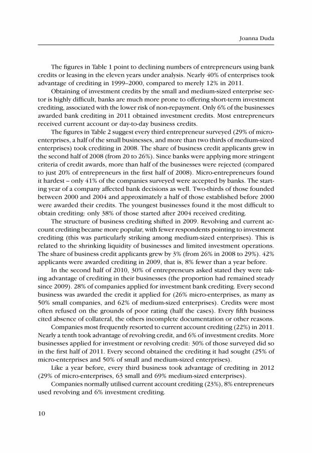
The figures in Table 1 point to declining numbers of entrepreneurs using bank credits or leasing in the eleven years under analysis. Nearly 40% of enterprises took advantage of crediting in 1999–2000, compared to merely 12% in 2011.
Obtaining of investment credits by the small and medium-sized enterprise sec-tor is highly difficult, banks are much more prone to offering short-term investment crediting, associated with the lower risk of non-repayment. Only 6% of the businesses awarded bank crediting in 2011 obtained investment credits. Most entrepreneurs received current account or day-to-day business credits.
The figures in Table 2 suggest every third entrepreneur surveyed (29% of micro-enterprises, a half of the small businesses, and more than two thirds of medium-sized enterprises) took crediting in 2008. The share of business credit applicants grew in the second half of 2008 (from 20 to 26%). Since banks were applying more stringent criteria of credit awards, more than half of the businesses were rejected (compared to just 20% of entrepreneurs in the first half of 2008). Micro-entrepreneurs found it hardest – only 41% of the companies surveyed were accepted by banks. The start-ing year of a company affected bank decisions as well. Two-thirds of those founded between 2000 and 2004 and approximately a half of those established before 2000 were awarded their credits. The youngest businesses found it the most difficult to obtain crediting: only 38% of those started after 2004 received crediting.
The structure of business crediting shifted in 2009. Revolving and current ac-count crediting became more popular, with fewer respondents pointing to investment crediting (this was particularly striking among medium-sized enterprises). This is related to the shrinking liquidity of businesses and limited investment operations. The share of business credit applicants grew by 3% (from 26% in 2008 to 29%). 42% applicants were awarded crediting in 2009, that is, 8% fewer than a year before.
In the second half of 2010, 30% of entrepreneurs asked stated they were tak-ing advantage of crediting in their businesses (the proportion had remained steady since 2009). 28% of companies applied for investment bank crediting. Every second business was awarded the credit it applied for (26% micro-enterprises, as many as 50% small companies, and 62% of medium-sized enterprises). Credits were most often refused on the grounds of poor rating (half the cases). Every fifth business cited absence of collateral, the others incomplete documentation or other reasons.
Companies most frequently resorted to current account crediting (22%) in 2011. Nearly a tenth took advantage of revolving credit, and 6% of investment credits. More businesses applied for investment or revolving credit: 30% of those surveyed did so in the first half of 2011. Every second obtained the crediting it had sought (25% of micro-enterprises and 50% of small and medium-sized enterprises).
Like a year before, every third business took advantage of crediting in 2012 (29% of micro-enterprises, 63 small and 69% medium-sized enterprises).
Companies normally utilised current account crediting (23%), 8% entrepreneurs used revolving and 6% investment crediting.
11
The Role of Bank Credits in Investment Financing...
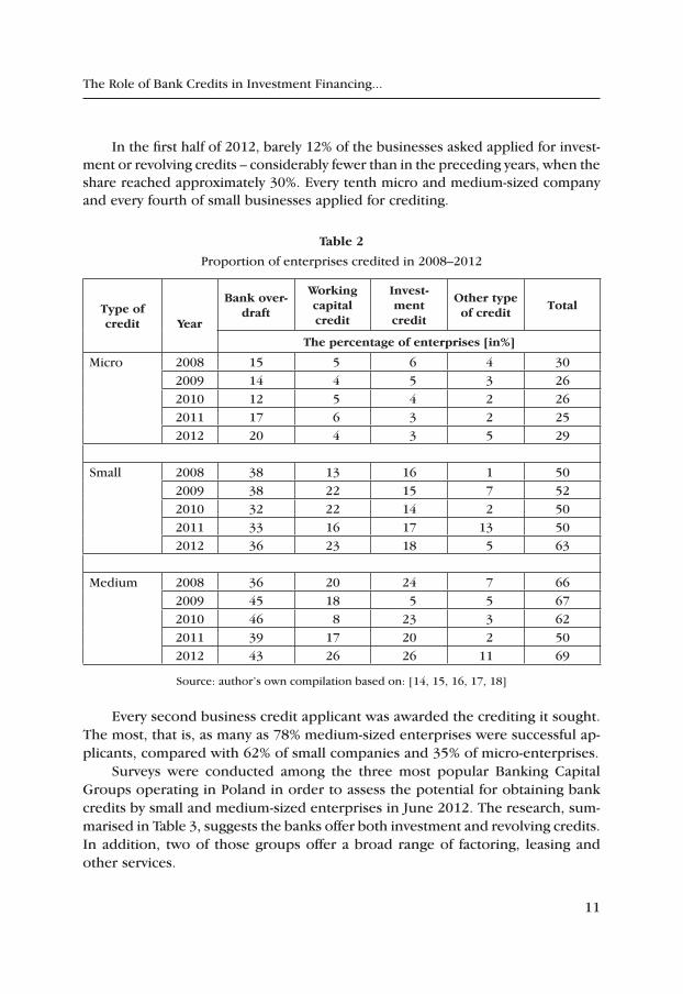
In the first half of 2012, barely 12% of the businesses asked applied for invest-ment or revolving credits – considerably fewer than in the preceding years, when the share reached approximately 30%. Every tenth micro and medium-sized company and every fourth of small businesses applied for crediting.
table 2
Proportion of enterprises credited in 2008–2012
type of credit Year
Bank over‑draft
Working capital credit
invest‑ment credit
Other type of credit
total
the percentage of enterprises [in%]
Micro 2008 15 5 6 4 302009 14 4 5 3 262010 12 5 4 2 262011 17 6 3 2 252012 20 4 3 5 29
Small 2008 38 13 16 1 502009 38 22 15 7 522010 32 22 14 2 502011 33 16 17 13 502012 36 23 18 5 63
Medium 2008 36 20 24 7 662009 45 18 5 5 672010 46 8 23 3 622011 39 17 20 2 502012 43 26 26 11 69
Source: author’s own compilation based on: [14, 15, 16, 17, 18]
Every second business credit applicant was awarded the crediting it sought. The most, that is, as many as 78% medium-sized enterprises were successful ap-plicants, compared with 62% of small companies and 35% of micro-enterprises.
Surveys were conducted among the three most popular Banking Capital Groups operating in Poland in order to assess the potential for obtaining bank credits by small and medium-sized enterprises in June 2012. The research, sum-marised in Table 3, suggests the banks offer both investment and revolving credits. In addition, two of those groups offer a broad range of factoring, leasing and other services.

12
Joanna Duda
table 3
Banking products offered to SME sector
type of service BZ WBK SA Bank Spółdzielczy pKO Bp SA
Working capital credit x x x
Investment credit x x x
Loan x - x
Factoring x - x
Leasing x - x
Deposit x - x
Bank account mainte-nance
x x x
Other - - x
Source: author’s own research
The banks declared offering credits for the SME sector yet, as the figures in Table 4 demonstrate, none provided investment crediting for micro-enterprises, which confirms the earlier proposition that micro-enterprises find bank investment crediting less accessible than small and medium-sized enterprises.
table 4
Beneficiaries of bank credits
type of enterprise BZ WBK SA Bank Spółdzielczy pKO Bp SA
Micro - - -
Small - x x
Medium x x x
Source: author’s own research
In their assessment of credit applications, banks primarily take into consid-eration credit histories, the key problem of the Polish SME sector, particularly of micro-enterprises which have normally operated for short period of time (Table 5). GUS informs approx. 50% of new SMEs operate for less than a year, with 75% collapsing in the first three years of business. The amount of collateral is an ad-ditional barrier to crediting.

13
The Role of Bank Credits in Investment Financing...
table 5
Elements in assessment of creditworthiness by banks
elements of credit‑worthiness examination
BZ WBK SA Bank Spółdzielczy pKO Bp SA
Credit history – x x
Possible collaterals x x x
Economic and financial situation
x x x
Other – entrepreneur’s assets
assessment of qualitative and
quantitative indi-cators
Source: author’s own research
Due to the low credit rating of the Polish SME sector, banks require collaterals of between 120% and 150% of credit value. In the opinion of banks included in Table 6, promissory notes, mortgage and pledge of chattels are credit collaterals of choice.
table 6
Means of collateral preferred by banks
Means of collateral BZ WBK SA Bank Spółdzielczy pKO Bp SA
Promissory note x X x
Mortgage x X x
Guarantee – – x
Alienation x -
Pledge of chattels x x x
Power of attorney to the account
– – x
Blocking of funds in bank accounts
– – x
Source: author’s own research
14
Joanna Duda
3.1. Bank credit interest in 2008–2012
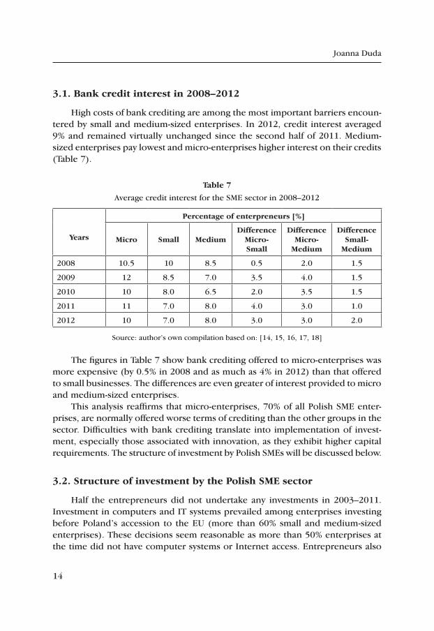
High costs of bank crediting are among the most important barriers encoun-tered by small and medium-sized enterprises. In 2012, credit interest averaged 9% and remained virtually unchanged since the second half of 2011. Medium-sized enterprises pay lowest and micro-enterprises higher interest on their credits (Table 7).
table 7
Average credit interest for the SME sector in 2008–2012
Years
percentage of enterpreneurs [%]
Micro Small MediumDifference
Micro‑Small
DifferenceMicro‑
Medium
Difference Small‑
Medium
2008 10.5 10 8.5 0.5 2.0 1.5
2009 12 8.5 7.0 3.5 4.0 1.5
2010 10 8.0 6.5 2.0 3.5 1.5
2011 11 7.0 8.0 4.0 3.0 1.0
2012 10 7.0 8.0 3.0 3.0 2.0
Source: author’s own compilation based on: [14, 15, 16, 17, 18]
The figures in Table 7 show bank crediting offered to micro-enterprises was more expensive (by 0.5% in 2008 and as much as 4% in 2012) than that offered to small businesses. The differences are even greater of interest provided to micro and medium-sized enterprises.
This analysis reaffirms that micro-enterprises, 70% of all Polish SME enter-prises, are normally offered worse terms of crediting than the other groups in the sector. Difficulties with bank crediting translate into implementation of invest-ment, especially those associated with innovation, as they exhibit higher capital requirements. The structure of investment by Polish SMEs will be discussed below.
3.2. Structure of investment by the polish SMe sector
Half the entrepreneurs did not undertake any investments in 2003–2011. Investment in computers and IT systems prevailed among enterprises investing before Poland’s accession to the EU (more than 60% small and medium-sized enterprises). These decisions seem reasonable as more than 50% enterprises at the time did not have computer systems or Internet access. Entrepreneurs also
15
The Role of Bank Credits in Investment Financing...
bought production plant and machinery, both new and second-hand. Investments into machinery of production parameters similar to those of the equipment already held, in the development of sales networks, improvement of services, purchase of state-of-the-art manufacturing plant and machinery were also noted in 2004. These investments were chiefly motivated by the desire to meet heavy competi-tion in the EU market [2].
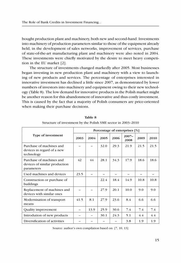
The structure of investments changed markedly after 2005. Most businesses began investing in new production plant and machinery with a view to launch-ing of new products and services. The percentage of enterprises interested in innovative investment has declined a little since 2007, as demonstrated by lower numbers of investors into machinery and equipment owing to their new technol-ogy (Table 8). The low demand for innovative products in the Polish market might be another reason for this abandonment of innovative and thus costly investment. This is caused by the fact that a majority of Polish consumers are price-oriented when making their purchase decisions.
table 8
Structure of investment by the Polish SME sector in 2003–2010
type of investment
percentage of enterprises [%]
2003 2004 2005 20062007–2008
2009 2010
Purchase of machines and devices in regard of a new technology
– – 32.0 29.3 21.9 21.5 21.5
Purchase of machines and devices of similar production parameters
42 44 28.1 34.3 17.9 18.6 18.6
Used machines and devices 23.5 – – – – – –
Construction or purchase of buildings
22.4 18.4 14.9 10.8 10.8
Replacement of machines and devices with similar ones
– – 27.9 20.1 10.0 9.0 9.0
Modernisation of transport means
41.5 8.1 27.9 23.6 8.4 6.6 6.6
Quality improvement – 13.9 25.9 30.6 7.4 7.4 7.4
Introdution of new products – – 30.1 24.3 5.1 4.4 4.4
Diversification of activities – – – – 3.8 1.9 1.9
Source: author’s own compilation based on: [7, 10, 13]
16
Joanna Duda
Investments are one of the key ways of realising business growth. The need for investments is motivated by escalating competition in the market, changing environment and growing customer expectations. At a time of rapid technical progress and market competition, features such as innovation, modernising spirit and flexibility provide opportunities for survival and development. These char-acteristics are implemented via investment which assures continuing operation and effective competition [19].
4. Accessibility of financing for Lesser poland SMe sector in 2010–2012
Results of the author’s research into a sample of 100 Lesser Poland micro-enterprises in 2009–2011 will be presented in this section.
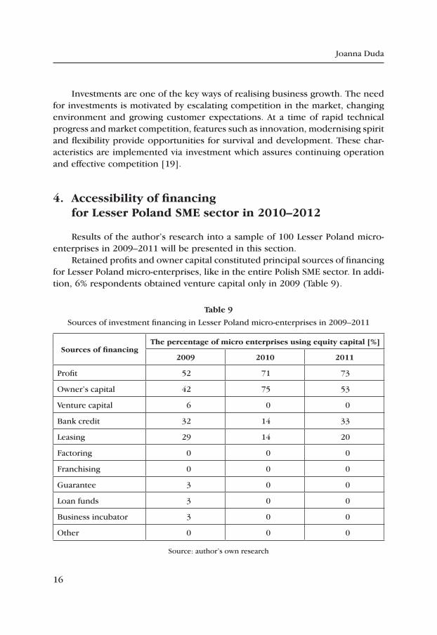
Retained profits and owner capital constituted principal sources of financing for Lesser Poland micro-enterprises, like in the entire Polish SME sector. In addi-tion, 6% respondents obtained venture capital only in 2009 (Table 9).
table 9
Sources of investment financing in Lesser Poland micro-enterprises in 2009–2011
Sources of financingthe percentage of micro enterprises using equity capital [%]
2009 2010 2011
Profit 52 71 73
Owner’s capital 42 75 53
Venture capital 6 0 0
Bank credit 32 14 33
Leasing 29 14 20
Factoring 0 0 0
Franchising 0 0 0
Guarantee 3 0 0
Loan funds 3 0 0
Business incubator 3 0 0
Other 0 0 0
Source: author’s own research
17
The Role of Bank Credits in Investment Financing...
The figures in Table 9 indicate that bank crediting was only employed by a few entrepreneurs, which is also the case for the Polish SME sector as a whole. Only a few obtained pledges from credit pledge funds, aid from enterprise think-tanks was utilised to a limited extent as well. Only banking credits and leasing were taken advantage of among third-party capitals.
Significantly (18%) fewer businesses used bank crediting and 15% fewer financed their investments with leasing in 2010 when compared to 2009. None employed venture capital funding, aid from credit pledge funds or enterprise think-tanks. The share of entrepreneurs using bank credits rose again to 33% and those taking advantage of leasing to 20% in 2011, on the other hand.
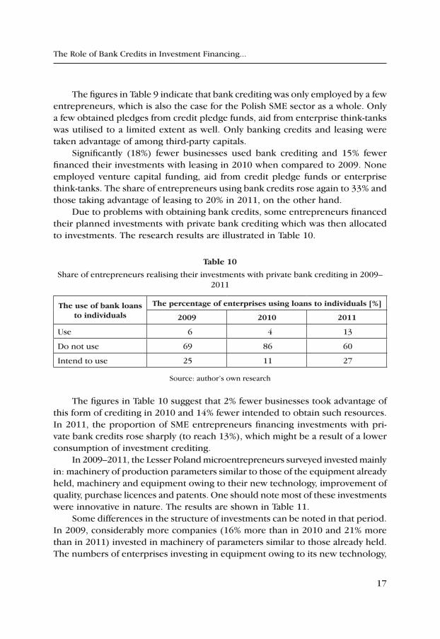
Due to problems with obtaining bank credits, some entrepreneurs financed their planned investments with private bank crediting which was then allocated to investments. The research results are illustrated in Table 10.
table 10
Share of entrepreneurs realising their investments with private bank crediting in 2009–2011
the use of bank loans to individuals
the percentage of enterprises using loans to individuals [%]
2009 2010 2011
Use 6 4 13
Do not use 69 86 60
Intend to use 25 11 27
Source: author’s own research
The figures in Table 10 suggest that 2% fewer businesses took advantage of this form of crediting in 2010 and 14% fewer intended to obtain such resources. In 2011, the proportion of SME entrepreneurs financing investments with pri-vate bank credits rose sharply (to reach 13%), which might be a result of a lower consumption of investment crediting.
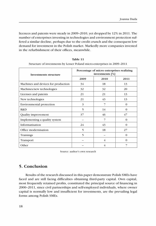
In 2009–2011, the Lesser Poland microentrepreneurs surveyed invested mainly in: machinery of production parameters similar to those of the equipment already held, machinery and equipment owing to their new technology, improvement of quality, purchase licences and patents. One should note most of these investments were innovative in nature. The results are shown in Table 11.
Some differences in the structure of investments can be noted in that period. In 2009, considerably more companies (16% more than in 2010 and 21% more than in 2011) invested in machinery of parameters similar to those already held. The numbers of enterprises investing in equipment owing to its new technology,
18
Joanna Duda
licences and patents were steady in 2009–2010, yet dropped by 12% in 2011. The number of enterprises investing in technologies and environment protection suf-fered a similar decline, perhaps due to the credit crunch and the consequent low demand for investment in the Polish market. Markedly more companies invested in the refurbishment of their offices, meanwhile.
table 11
Structure of investments by Lesser Poland micro-enterprises in 2009–2011
investments structure
percentage of micro enterprises realizing investments [%]
2009 2010 2011
Machines and devices for production 34 18 13
Machines/new technologies 32 32 20
Licenses and patents 21 21 13
New technologies 21 43 13
Environmental protection 3 7 0
R&D 5 14 0
Quality improvement 37 46 47
Implementing a quality system – 7 0
Informatisation 24 43 0
Office modernisation 5 18 27
Trainings 5 – 0
Transport – 4 0
Other – 4 7
Source: author’s own research
5. conclusion
Results of the research discussed in this paper demonstrate Polish SMEs have faced and are still facing difficulties obtaining third-party capital. Own capital, most frequently retained profits, constituted the principal source of financing in 2000–2011, since civil partnerships and self-employed individuals, where owner capital is normally low and insufficient for investments, are the prevailing legal forms among Polish SMEs.
19
The Role of Bank Credits in Investment Financing...
Numbers of enterprises taking advantage of bank credits markedly varied in the eleven years under analysis (Table 1). Nearly a quarter of entrepreneurs took bank crediting in the late 1990s and in 2000 yet, due to high rates of unpaid cred-its, banks applied palpably more stringent crediting policies, which has sharply reduced the number of entities utilising this source.
An analysis of available data suggests banks are more willing to award revolv-ing and current account credits to SME entrepreneurs. The regularity can also be observed that the smaller a business, the poorer terms of credit it is offered (Table 2). It appears that most commercial banks do not supply crediting to micro-enterprises. In the face of the high risk posed by this group, banks require three years of credit histories and collateral to 120%-150% of the credit value.
High costs of obtaining bank credits are another barrier to small and medium-sized enterprises. The figures in Table 7 suggest that credits offered to micro-enterprises bear higher interest than those available to small and medium-sized enterprises. Some micro-entrepreneurs attempt to bridge this capital gap with crediting for private individuals (Table 10).
The restricted access to long-term bank crediting directly translates into the structure of investments and the degree of their innovative nature. In 2003–2011, more than a half of SME entrepreneurs failed to undertake any investment projects. Merely 20% of those who did invested in broadly-defined innovation, a principal factor underpinning the long-term competitive advantage of market enterprises.
references
[1] Berger A.N., Klapper L.F., Udell G.F., The ability of banks to lend informa-tionally opaque small businesses, “Journal of Banking & Finance”, Issue 25, 2001.
[2] Duda J., Decyzje inwestycyjne przedsiębiorstw polskich z sektora MSP, in: Prace Naukowe Uniwersytetu Ekonomicznego, Wydawnictwo Uniwersytetu Ekonomicznego, Wrocław, 2009.
[3] Duda J., Strategie finansowania działalności inwestycyjnej polskich MSP na rynku Unii Europejskiej, Zeszyty Naukowe Uniwersytetu Szczecińskiego 685, Finanse, Rynki Finansowe, Ubezpieczenie nr 46, Szczecin 2011,
[4] Flejterski S., Specyfika i źródła finansowania mikro- i małych przedsiębiorstw, in: Zarządzanie finansami. Zarządzanie i kreowanie wartości, ed. D. Za-rzecki, Wydawnictwo Naukowe Uniwersytetu Szczecińskiego, Szczecin 2007.
[5] Łuczka T., Kapitał obcy w małym i średnim przedsiębiorstwie, Wydawnictwo Naukowe PWN, Warszawa–Poznań 2001.
[6] Michalczewski A., Kredyty inwestycyjne. Sposoby zabezpieczania przed ryzy-kiem stopy procentowej i ryzykiem walutowym, in: Finansowanie rozwoju przedsiębiorstwa – studia przypadku, red. M. Panfil, Difin, Warszawa 2008.
Joanna Duda
[7] Monitoring kondycji sektora MSP, PKPP Lewiatan, Warszawa 2004, 2005, 2006, 2007, 2009, 2010, 2011, 2012.
[8] Przepióra P., Koszt kredytu w małych i średnich firmach a harmonogram jego spłaty, Zeszyty Naukowe Uniwersytetu Szczecińskiego, Ekonomiczne problemy usług nr 51, Szczecin 2010.
[9] Raport o stanie sektora małych i średnich przedsiębiorstw w Polsce w la-tach 2006–2007, ed. A. Żołnierski, P. Zadura-Lichota, Polska Agencja Rozwoju Przedsiębiorczości, Warszawa 2008.
[10] Raty równe i raty malejące kredytu hipotecznego – jakie wybrać?, protokół dostępu: http:// www.finansegoc.pl/poradnik.php?art=2 [04.12.2009] lub Raty malejące czy stałe?, protokół dostępu: http://www.muratordom.pl/prawo-i-pieniadze/kredyty-i-pozyczki/raty-malejace-czy-stale_,7269_3916.htm [04.12.2009].
[11] Rutkowski A., Zarządzanie finansami, PWE, Warszawa 2003.[12] Starczewska-Krzysztoszek M., Bariery rozwoju małych i średnich przedsię-
biorstw w Polsce, in: „infos”, Biuro Analiz Sejmowych, nr 4, 2008.[13] Trendy rozwojowe sektora MSP w ocenie przedsiębiorców w pierwszej po-
łowie 2012 roku, MG DPiA, nr 2/2012, Warszawa 2012.[14] Trendy rozwojowe sektora MSP w ocenie przedsiębiorców w pierwszej po-
łowie 2011 roku, MG DPiA, nr 2/2011, Warszawa 2011.[15] Trendy rozwojowe sektora MSP w ocenie przedsiębiorców w pierwszej po-
łowie 2010 roku, MG DPiA, nr 2/2010, Warszawa 2010.[16] Trendy rozwojowe sektora MSP w ocenie przedsiębiorców w pierwszej po-
łowie 2009 roku, MG DPiA, nr 2/2009, Warszawa 2009.[17] Trendy rozwojowe sektora MSP w ocenie przedsiębiorców w pierwszej po-
łowie 2008 roku, MG DPiA, nr 2/2008, Warszawa 2008.[18] Vos E., Jia-Yuh Yeh A., Carter S., Tagg S., The happy story of small business
financing, “Journal of Banking & Finance” Issue 31, 2007.[19] Wolak-Tuzimek A., Działalność inwestycyjna polskich przedsiębiorstw,
in: Zeszyty Naukowe Uniwersytetu Szczecińskiego 639, Zarządzanie Finan-sami, Inwestycje, Wycena Przedsiębiorstw, Zarządzanie Wartością, Szczecin 2011.
[20] Wolański R., Relacje między bankami a małymi i średnimi przedsiębiorstwa-mi, w: Prace Naukowe Katedry Ekonomii i Zarządzania Przedsiębiorstwem, ed. F. Bławat, t. IV, Gdańsk 2005.
21
Managerial Economics2013, No. 13, pp. 21–44
http://dx.doi.org/10.7494/manage.2013.13.21
Henryk Gurgul*, Roland Mestel**, Robert Syrek***
the testing of causal Stock returns‑trading Volume Dependencies with the Aid of copulas
1. introduction
Market participants usually think that a share price reflects investors’ predic-tions about the future performance of a company. These expectations are based on available information about the company. The release of new information forces investors to change their expecta tions about the future performance of the company. New announcements are the main source for price fluctuations. Since investors evaluate the content of new information differently, prices may remain constant even though new information is important for the market. This can be the case if some investors think that the news is good, whereas others understand the same announcements quite differently. The direction of movements of prices depends on the average reaction of investors to news.
It is obvious that share prices can be observed if there is a positive trading volume. As with prices, trading volume and its changes react to the available set of important information on the market. Trading volume reacts in a different way in comparison to stock prices. A change in investors’ expectations always leads to a rise in trading volume. The trading volume adjusts the sum of investors’ reactions to news.
A real answer to the question whether a knowledge of one variable (e.g. vola-tility) can improve short–run forecasts of other variables is essential not only for analysts but also for market participants. Thus, in recent years both researchers
* AGH University of Science and Technology in Cracow, Department of Applications of Mathematics in Economics, e–mail: [email protected].
Financial support for this paper from the National Science Centre of Poland (Research Grant DEC-2012/05/B/HS4/00810) is gratefully acknowledged.
** University of Applied Sciences Joanneum in Graz, Department of Banking and Insurance, e-mail: [email protected]
*** Jagiellonian University in Cracow, Institute of Economics and Management, e–mail: [email protected]
22
Henryk Gurgul, Roland Mestel, Robert Syrek
and investors have focused on the links between trading volume, stock return and return volatility. Most early empirical examinations have been concerned the contemporaneous relationship between price changes and trading volume.
Both from a theoretical and practical point of view the dynamic relationship between returns, return volatility and trading volume is more interesting than the contemporaneous one. One of the most important and useful topics in empiri-cal economics is an examination of the causal relationship between the variables in question. The notion of causality was introduced by Granger [20]. It is based on the idea that the past cannot be determined by the present or future. Thus, if one event is observed before another event, causality can only take place from the first event to the second one.
Brief information about some aspects of causality and the background litera-ture contributions will be given in the next section. The concepts of nonlinear causality and Bernstein copulas are outlined in the third section. Data descrip-tion and the estimation method of realized volatility are presented in the fourth section. The empirical results are discussed in the fifth section. Brief conclusions and outlook are given in the last part of the paper.
2. Literature review
Karpoff [30] in his survey of early research about price-volume relations citied important reasons for regarding price-volume dependencies. This permits zn insight into the structures of financial markets, and an understanding of the information arrival process especially how information is disseminated among market participants. It is strictly related to two hypotheses: the mixture of distribu-tions hypothesis (MDH), Clark [13], Epps and Epps [17], Tauchen and Pitts [44] and Harris [28] and the sequential information arrival hypothesis by Copeland [14] and Tauchen and Pitts [44]. The knowledge of price-volume relations is also useful in technical analysis and it is important with respect to investigations of options and futures markets and in fashioning new contracts.
One of the most useful approaches in the research concerning return-trading volume interrelations is the concept of Granger causality [20]. Causality in the Granger sense can be understood as a kind of conditional dependency. Using this causality methodology we can check if the past values of one stationary variable is helpful in predicting the future values of another one or not. In most early papers concerned with causal dependencies linear vector autoregression models are used. The significance of coefficient estimates of a potentially causal variable means the existence of causality running from this variable to the endogenous variable. However, in the case of the nonstationarity of the time series under study
23
The Testing of Causal Stock Returns-Trading Volume Dependencies...
to causality can be spurious (comp. Granger and Newbold [21], Phillips [38]). In the case of cointegration VECM can be applied for causality testing. If one finds the respective coefficient of error correction to be not-negative, then it can be concluded that there is no stable and long-run relationship.
Another serious problem concerning the linear approach to testing for causal-ity is the low power of the tests needed to detect some kinds of nonlinear causal relationships. This problem is raised in contributions which are concerned with nonlinear causality tests (see e.g. Abhyankar [1] and Asimakopoulos [2]). The starting point for further investigations was the nonparametric statistical method for uncovering nonlinear causal effects presented by Baek and Brock [7]. In order to detect causal relations the authors used the correlation integral, an estimator of spatial probabilities across time based upon the closeness of points in hyperspace.
The concept by Hiemstra and Jones [29] improves the small-sample proper-ties of the causality test and relaxes the assumption that the series to which the test is applied are i.i.d. The authors conducted some Monte Carlo simulations and proved the robustness of their test for the presence of structural breaks in the series. They also checked contemporaneous correlations in the errors of the VAR model in order to filter out linear cross- and auto-dependence.
Diks and Panchenko [15, 16] noticed the fact that the null hypothesis in the HJ (Hiemstra and Jones) test is generally not equivalent to Granger non-causality. The authors developed their own test with better performance than the HJ one, especially in terms of over-rejection and size distortion, which are frequently reported for the HJ test. The authors gave some recommendations, including bandwidth adaptation for ARCH type processes. In this case, the optimal band-width can be expressed in terms of the ARCH model coefficient.
There are also a few papers e.g. Sims et al. [41], Toda and Yamamoto [45] which demonstrated that the asymptotic distribution theory is not a proper basis for testing the causality of integrated variables by mean of the VAR model. This also holds true in a case where the variables are cointegrated. Therefore, an alter-native concept of causality testing was developed based on a Wald test statistic.
Almost all of the papers analyzed the dynamic links of indexes and individual companies listed in these indexes from highly developed stock markets.
Gurgul et al. [25] investigated the causal relationships between trading volume and stock returns and return volatility for the Warsaw Stock Exchange. Applying the linear Granger causality test, the contributors observed a significant causal relationship between returns and trading volume in both directions and linear Granger causality from return volatility to trading volume. In addition, their findings showed that a knowledge of past stock price movements on the German as well as the US stock market supported short–run predictions of current and future trading volume of the companies from the WSE.
24
Henryk Gurgul, Roland Mestel, Robert Syrek
Gurgul et al. [23] in a contribution based only on the traditional linear ap-proach concluded that short-run forecasts of current or future stock returns cannot be improved by a knowledge of recent volume data and vice versa.
The linear and nonlinear causality of companies listed in, DAX index was investigated by Gurgul and Lach [22]. They used daily data at close from the time period January 2001- November 2008. The contributors presented the results of linear and nonlinear testing for causality. While for testing of the nonlinear causality the Diks and Panchenko test was used the linear dependencies were checked by traditional Vector Autoregression Models and by the model derived by Lee and Rui [31]. The contributors confirmed the hypothesis that traditional linear causality tests often fail to detect some kinds of nonlinear relations, while nonlinear tests do not. In many cases the test results obtained by use of empirical data and simulation confirmed a bidirectional causal relationship while a linear test did not detect such causality at all.
A hypothesis on dynamic interdependencies between returns and trading volume is the high volume premium hypothesis. High trading volume of a stock implies that investors focus on that stock. This implies that such a stock seems to be more interesting to potential investors which is whythe stock prices tend to increase. This hypothesis was tested by Gervais et al. [19]. The contributors checked this hypothesis for companies listed on the NYSE. The results are in line with the high volume premium hypothesis since the authors observed that high trading volume precedes high returns while small trading volume precedes low returns.
Gurgul and Wójtowicz [25], taking into account event study methodology defined an event as the appearance of extreme high trading volume. The authors tested the high volume premium hypothesis for companies listed on the WSE. The results were in line with the high volume premium conjecture since the oc-currence of high trading volume implied high returns (especially in the case of small companies) in the following days, especially one day after. The results not only supported the high trading volume premium hypothesis but also suggested the construction of profitable investment strategies. In addition, in the case of small trading volume the mean abnormal returns were not statistically significant.
The papers above were concerned with dynamic dependencies between returns, return volatility and trading volume on the basis of daily data. However, these dependencies are much more interesting for high frequency data. In all papers reviewed absolute values or squared stock returns were applied as proxies for volatility. There are few papers dealing with intraday data when links between returns, return volatility and trading volume are examined.
Rossi and Magistris [40] investigated the relationship between realized vola-tility and trading volume. They showed that volume and volatility exhibit long
25
The Testing of Causal Stock Returns-Trading Volume Dependencies...
memory but they are not driven by the same latent factor as suggested by frac-tional cointegration analysis. They used the fractional cointegration VAR models of Nielsen and Shimotsu [37], which extend the analysis of Robinson and Yajima [39] to stationary and nonstationary time series as well. They found that past (filtered) log-volume has a positive effect on current filtered log-volatility and current log-volume as well. Their analysis was complemented by using copulas in order to measure the degree of tail dependence. The series of log-volume and log-volatility are found to be dependent in extreme values. Luu and Martens [33] conducted some tests of the mixture of distributions hypothesis using realized volatility and found bidirectional causality of realized volatility and the trading volume of S&P500 index future contracts, whereas when using daily stock returns the MDH was not supported. The results of long memory analysis suggested that trading volume and volatility share the same degree of long-run dynamics, which supported the Bollerslev and Jubinski [11] version of MDH. Fleming and Kirby [18] also considered the Bollerslev and Jubinski [11] interpretation of MDH but they used fractionally-integrated time series models to investigate the joint dynamics of trading volume and volatility. The contributors examined this issue using more precise volatility estimates obtained using high-frequency returns (i.e. realized volatilities). Their results indicated that both volume and volatil-ity displayed long memory. However they rejected the hypothesis that the two series shared a common order of fractional integration for a fifth of the firms in their sample. Moreover, the authors found a strong correlation between innova-tions in volume and volatility. The contributors draw the conclusion that trading volume can be used to obtain more precise estimates of daily volatility for cases in which high-frequency returns are unavailable. Bouezmarni et al. [12] derived a nonparametric test based on Bernstein copulas and tested on the basis of high frequency data for causality between stock returns and trading volume. The con-tributors proved, that at a 5% significance level, the nonparametric test rejected clearly the null hypothesis of non-causality from returns to volume, which is in line with the conclusion which followed from the linear test. Further, their non-parametric test also detects a non-linear feedback effect from trading volume to returns at a 5% significance level.
In the next part of this paper in order to check links between the financial variables under study realized volatility will be used as a proxy for volatility.
3. Nonlinear causality and Bernstein copulas
Now, we will present an extension of the Granger causality notion taking into account three variables X, Y and Z. Variable Z is in a causal relation to variable Y
26
Henryk Gurgul, Roland Mestel, Robert Syrek
in the Granger sense if the current values of the variable Y can be forecasted more precisely by means of the known past values of variable Z, and those of auxiliary variable X, than in the case where the values of variable Z are not involved in the forecasting process.
In the recent literature on nonlinear dependencies in the sense of Granger causality nonparametric tests are used for the conditional independence of ran-dom variables. The conditional independence of random variables implies a lack of causality in the Granger sense. Linton and Gozalo [32] tested conditional in-dependence by mean of a test statistic based on empirical distributions. Su and White [42] derived a test based on smoothed empirical likelihood functions and in the year 2007 developed a nonparametric test for the conditional independence of distributions. To this end, they applied conditional characteristic functions. The test for conditional independence by Su and White [43] is based on a ker-nel estimation of conditional distributions f(y|x) and f(y|x, z) if the null holds true than the last functions are equal. The serious drawback of this test is the restriction of the sum of dimensions of variables X, Y, Z to seven. In addition, it is necessary to define a weight function for Hellinger distance which is needed to measure the distance between the conditional distributions. The contributors applied their test to examine Granger non-causality in exchange rates. These drawbacks were addressed by Bouezmarni et al. [12]. We use their approach and methodology in the empirical part of this paper. The causality test applied for the detection of nonlinear causality is based on Bernstein copulas, which are presented in the next section.
3.1. Bernstein copulas
The estimator of density of a Bernstein copula in g = (g1, g2, g3) is determined by the expression:
c g g gT
K g GXYZ
t
T
k t^ ^, , , ,( )1 2 3
1
1( ) ==∑
where G G G Gt t t t^ ^ ^ ^( , , )= 1 2 3 stands for the vector ( , , ).^ ^ ^
F X F Y F ZX t Y t Z t( ) ( ) ( )The kernel Kk = (g, G^t) can be calculated by use of the binomial distributions:
p gk
vg gv j
jjv
j
k v
j
j j( ) =−
−( ) − −1
11
for vj = 0, ..., k-1 and j = 1, 2, 3.

27
The Testing of Causal Stock Returns-Trading Volume Dependencies...
Assume AG v G Bt t v^ ^, =
∈{ }1 to be the characteristic (indicator) function of set BV
which is defined as
Bvk
vk
vk
vk
v
k
v
kv = +
× +
×+
1 1 2 2 3 31 1 1, , , .
The kernel can be written as
K g G k A p gk t
v
k
v
k
v
k
G v jv j
tj
( ), .^
^ ,= ( )
=
−
=
−
=
−
=∑∑∑ ∏3
0
1
0
1
0
1
1
3
1 2 3
One can estimate a kernel Kk(g, G^t) by the use of the density function of Beta distributions with parameters vj + 1 and k - vj:
K g G A B g v k vk t
v
k
v
k
v
k
G v jj j
t
( ), ( , ,^
^ ,= + −
=
−
=
−
=
−
=∑∑∑ ∏1 2 30
1
0
1
0
1
1
3
1 jj ).
In the case of a two-dimensional copula the last expression for variables X and Y is given by
c g gT
K g GXY
t
T
k t^ ^, , ,( )1 2
1
1( ) ==∑
where G G G F X F Yt t t X t Y t^ ^ ^ ^ ^( , ( , ))= = ( ) ( )1 2 .
In addition
Bvk
vk
vk
vkv = +
× +
1 1 2 21 1, ,
and
K g G k A p gk t
v
k
v
k
G vj
v jv
k
vt j
( , )^
^ ,= ( ) =
=
−
=
−
= =
−
=∑∑ ∏ ∑2
0
1
0
1
1
2
0
1
1 2 1 2 00
1
1
2
1k
G vj
j j jA B g v k vt
−
=∑ ∏ + −
^ ,( , , ).
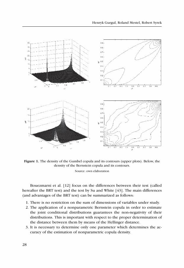
In the above equation the number k is the only parameter which should be set before the computations. This parameter stands for the number of „picks” of two dimensional distribution for which the density function is smoothed. It is obvious that the accuracy tends to increase as k rises. Figure 1 demonstrates a method for the nonparametric estimation of a Gumbel copula by use of a Bernstein copula. Therefore, 1000 realizations from a Gumbel copula with parameter 2 were gener-ated. Next for k = =2 1000 63 the density function*, was estimated by means of a nonparametric estimator based on binomial distributions.
* x denotes the integer part of the real number x.
28
Henryk Gurgul, Roland Mestel, Robert Syrek
Figure 1. The density of the Gumbel copula and its contours (upper plots). Below, the density of the Bernstein copula and its contours.
Source: own elaboration
Bouezmarni et al. [12] focus on the differences between their test (called hereafter the BRT test) and the test by Su and White [43]. The main differences (and advantages of the BRT test) can be summarized as follows:
1. There is no restriction on the sum of dimensions of variables under study.2. The application of a nonparametric Bernstein copula in order to estimate
the joint conditional distributions guarantees the non-negativity of their distributions. This is important with respect to the proper determination of the distance between them by means of the Hellinger distance.
3. It is necessary to determine only one parameter which determines the ac-curacy of the estimation of nonparametric copula density.
29
The Testing of Causal Stock Returns-Trading Volume Dependencies...
The contributors demonstrated by means of simulation studies that their test has appropriate power and allows a recognition of different nonlinear depen-dencies between variables. By means of simulation exercises they also supplied evidence for the uselessness of a classic linear causality test for the detection of causal dependencies between nonlinear processes. The authors applied their test in an examination Granger non-causality between many macroeconomic and financial variables.
3.2. Nonlinear causality versus conditional dependence
Let ′ ′ ′( )∈ × × = …{ }X Y Z t Tt t td d d, , , 1 2 3 1 be a realization of the stochastic
process in d, where d = d1 + d2 + d3 with joint distribution FXYZ and density func-tion fXYZ. The test of conditional independence between variables Y and Z under condition X can be written down for density functions as (Bouezmarni et al. [12]):
H P f y x z f y x yY X Z Y Xd
0 1 2: , , ,| , || |( ) = ( )( ) = ∀ ∈ (1)
H P f y x z f y x yY X Z Y Xd
1 1 2: , , ,| , || | for( ) = ( )( ) < ∈ (2)
where f⋅ ⋅ ⋅ ⋅( )| | stands for the conditional density function.
It is worth noting that a lack of causality in the Granger sense can be under-stood as conditional independence. Let (Y, Z)′ be a Markov process of order 1. Variable Z does not cause variable Y in the Granger sense if and only if the fol-lowing null hypothesis holds true:
H P f y y z f y yY X Z t t t Y X t t0 1 1 1 1: , ,| , || |− − −( ) = ( )( ) =
i.e. y = yt, x = yt-1, z = zt-1, for d1 = d2 = d3 = 1.
For the sake of simplicity of notation we assume di = 1 for i = 1, 2, 3. Taking into account this notation the well-known Sklar theorem can be put in the form:
F x y z C F x F y F zXYZ XYZ X Y Z, , , ,( ) = ( ) ( ) ( )( ) .
The respective density function fXYZ is given by the equation
f x y z f x f y f z c F x F y F zXYZ X Y Z XYZ X Y Z, , , , ,( ) = ( ) ( ) ( ) ( ) ( ) ( )( )where cXYZ is the density function of copula CXYZ.
30
Henryk Gurgul, Roland Mestel, Robert Syrek
The null hypothesis (1) can be expressed by means of the copula notion in the following form:
H P c F x F y F z c F x F y c F x F zXYZ X Y Z XY X Y XZ X Z0 : , , , ,( ) ( ) ( )( ) = ( ) ( )( ) ( ) ( )(( )( ) = ∀ ∈1, y
while alternative hypothesis (2) fulfills the inequality:
H P c F x F y F z c F x F y c F x F zXYZ X Y Z XY X Y XZ X Z1 : , , , ,( ) ( ) ( )( ) = ( ) ( )( ) ( ) ( )(( )( ) < 1
for y∈, where cXY and cXZ stand for densities of copulas of two dimensional distributions (X, Y) and (X, Z). The test statistics suggested by Bouezmarni et al. (2012) are based on the Hellinger distance between two distributions i.e. the density of the copula cXYZ and the product of the densities of copulas cXY and cXZ. This measure
H c Cc u v c u w
c F x F y F zXY XZ
XYZ X Y Z
,, ,
, ,,
( ) = −( ) ( )( ) ( ) ( )( )
[ ]∫
0 1 3
1
( )2
dC u v wXYZ , , . (3)
is equal to zero if the null hypothesis holds true. The distance (3) exhibits important advantages. First of all, it is symmetric
and invariant with respect to monotone transformations. In addition, it is not sensitive to outliers, because their weights are lower than the weights of other observations. For empirical data the Hellinger distance (3) can be estimated by means of the following formula:
H H c Cc u v c u w
c u v wT
XY XZ
XYZ
^ ^^ ^
^
( ,( , ) ( , )
( , , ))
,
= = −
[ ]∫
0 1 3
1
=
2
dC u v wXYZ( , , )
= −( ) ( ) ( ) ( )
=∑1
11T
c F X F Y F F X F Z
ct
TXY X T Y T XZ X T Z T
XYZ
^ ^ ^ ^ ^ ^
^
( , ) ( , )
( FF X F Y F ZX T Y T Z T^ ^ ^, , )
,( ) ( ) ( )
2
where F^.(.) is the empirical form of marginal distribution F.(.). In addition, the densities of copulas are estimated by means of nonparametric methods.
Test statistics (comp. Bouezmarni et al. [12]) for d1 = d2 = d3 = 1 is given by the formula:
BRTTk
H C T k B T k B T k B T k= − − − −
−− − − −
3 2
11 3 2
11
21
31 1 24
// /^ ^ ^ ^ ,
s (4)
31
The Testing of Causal Stock Returns-Trading Volume Dependencies...
where C13 3 2 3 2
2 2 4= = ( )− p s p/ /, / and
B TG G G G
ct
Tt t t t^
^ ^ ^ ^
^
( ( )) ( ( ))1
1 1
1
1 1
12 2 2
12
24 1 4 1= − + − −− −
=
− −
∑p p p
XXY t tG G( ),,
^ ^1 2
B TG G G G
ct
Tt t t t^
^ ^ ^ ^
^
( ( )) ( ( ))2
1 1
1
1 1
12 3 3
12
24 1 4 1= − + − −− −
=
− −
∑p p p
XXZ t tG G( ),,
^ ^1 3
B T
G Gt
T
t t
^
^ ^
/
( )
.31 2 1
11 1
1
1
=−
− −
=∑p
The densities cXYZ, cXY and cXZ are estimated by means of Bernstein copulas. Under the null hypothesis the test statistic is distributed asymptotically standard normal. The null hypothesis is rejected for a given significance level a iff BRT > za holds true where za denotes the critical value given in the tables of standard normal distribution. Taking into account that the test statistic is asymptotically normal, the contributors advise in the case of a finite sample the calculation of p-values by means of bootstrap methods. Classic bootstrap methods referring to empirical distribution cannot be applied. Therefore, Paparoditis and Politis [37] suggested a local bootstrap method for nonparametric kernel estimators. They take into account the fact that the densities of the variables are conditional. This method was applied by Bouezmarni et al. [12] and Su and White [43]. The p-values can be determined for the samples X Y Zt t t t
T* * *, ,( ){ }
=1 generated by bootstraping under
condition d1 = d2 = d3 = 1 in the following steps:
1. In the first step Xt* is generated by means of the kernel estimator:
f x T h f X x ht
T
t
~/ ,( ) = −( )( )− −
=∑1 1
1
where f stands for the density of one dimensional distribution.
For t = 1, ..., T the values of Yt* and Zt
* should be generated independently from conditional densities:
f y X
fY y
hf
X X
h
fX
t
s
T s s s
s
T t
~*
*
|( ) =
−( )
−( )
−
=
=
∑
∑
1
1
XX
hs*
,( )
32
Henryk Gurgul, Roland Mestel, Robert Syrek
f z X
fZ z
hf
X X
h
fX
t
s
T s s s
s
T t
~*
*
|( ) =
−( )
−( )
−
=
=
∑
∑
1
1
XX
hs*( )
.
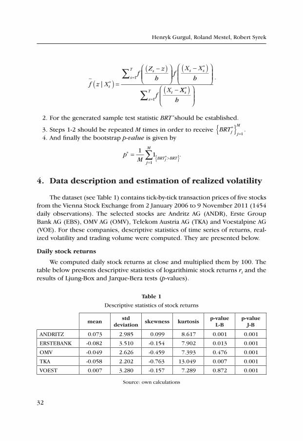
2. For the generated sample test statistic BRT *should be established.
3. Steps 1-2 should be repeated M times in order to receive BRTj j
M* .{ } =1
4. And finally the bootstrap p-value is given by
pM j
M
BRT BRTj
** .=
=>{ }∑1
11
4. Data description and estimation of realized volatility
The dataset (see Table 1) contains tick-by-tick transaction prices of five stocks from the Vienna Stock Exchange from 2 January 2006 to 9 November 2011 (1454 daily observations). The selected stocks are Andritz AG (ANDR), Erste Group Bank AG (EBS), OMV AG (OMV), Telekom Austria AG (TKA) and Voestalpine AG (VOE). For these companies, descriptive statistics of time series of returns, real-ized volatility and trading volume were computed. They are presented below.
Daily stock returns
We computed daily stock returns at close and multiplied them by 100. The table below presents descriptive statistics of logarithimic stock returns rt and the results of Ljung-Box and Jarque-Bera tests (p-values).
table 1
Descriptive statistics of stock returns
meanstd
deviationskewness kurtosis
p‑value L‑B
p‑value J‑B
ANDRITZ 0.073 2.985 0.099 8.617 0.001 0.001
ERSTEBANK -0.082 3.510 -0.154 7.902 0.013 0.001
OMV -0.049 2.626 -0.459 7.393 0.476 0.001
TKA -0.058 2.202 -0.763 13.049 0.007 0.001
VOEST 0.007 3.280 -0.157 7.289 0.872 0.001
Source: own calculations
33
The Testing of Causal Stock Returns-Trading Volume Dependencies...
The results confirmed the stylized facts about stock returns rt. The departure from normality is reflected in kurtosis and skewness. The null hypothesis about normality is rejected for all companies under study. In three cases we observe significant autocorrelation.
realized volatility
As a proxy of volatility in empirical investigations squared returns or absolute returns are used. For high frequency data a better alternative is realized volatility.
Suppose that pi,t is the logarithm of price (expressed in %) m times in day t in equal time intervals. The estimator of realized volatility is defined as
RV p p rti
m
i t i ti
m
i t= −( ) ==
−=
∑ ∑1
1
2
1
2, , , .
Under some regularity conditions RVt is a consistent estimator of integrated
volatility IV dst
t
t
s=+
∫1
2s , where in the stochastic differential equation dpt = mtdt +
+ stdWt for logarithmic prices, the variable st stands for volatility mt is drift and Wt is the Wiener process. Unfortunately in most cases RVt is a biased estimator because of autocorrelation in intraday data, caused by a microstructure noise ef-fect. The autocorrelation increases with rising frequency. In order to reduce the bias and mean squared error one can include covariances. Another solution is the choice of optimal sampling frequency (Bandi and Russell [3, 4, 6]), Zhang et al. [46], Hansen and Lunde [26, 27] and Oomen [36]).
Barndorff-Nielsen et al. [8, 9, 10] have introduced the class of realized kernel estimators. A survey of realized variance estimators can be found in Bandi and Russel [4] and McAleer and Medeiros [34].
In this paper we use a Newey-West estimator based on the Bartlett kernel for daily realized volatility (Hansen and Lunde [26]):
RV rk
qr rt
NW
i
m
i tk
q
ii t i k t= + −
+
= = =
−
+∑ ∑ ∑1
2
1 1
2 11, , , .
m k
This estimator has many advantages. However, it does not take into account volatility between the close of a session and the opening of the session next day. Therefore, it is necessary to add to RVt
NW a square of return computed for the price at close and the price at open denoted by rCOt.
Hansen and Lunde [26] introduced the realized volatility estimation method for a whole day. In order to minimize the mean square error the linear combina-tion of r2
ZOt and RVtNW was taken into account. The optimal, conditionally unbiased,
minimum variance estimator of realized volatility in the class of linear estimators is:
RV r RVt COt tNW
~= +w w1
22 ,
34
Henryk Gurgul, Roland Mestel, Robert Syrek
where
w j mm1
0
1
1= −( ) , w j mm2
0
2
=
and
j m h m m hm h m h m m h
= −− −22
12
1 2 12
22
12
12
22
1 2 122
and rCOt is the close-to-open log-return.
The parameter ϕ gives a relative importance factor that indirectly stands for a portion of the volatility observed during the session. The parameters in the equations above are computed as follows:
m m m02
12
2= +( ) = ( ) = ( )E r RV E r E RVCOt tNW
COt tNW, ,
h h h12 2
22
122= ( ) = ( ) = ( )var r var RV cov r RVCOt t
NWCOt t
NW, , , .
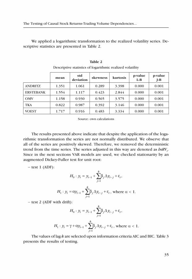
Based on high frequency data, by applying these formulae to opening and closing prices the time series of realized volatility were derived. In the Newey-West estimator the time lags were chosen in order to minimize the mean square error. In addition, for the companies listed on Vienna Stock Exchange an optimal frequency parameter m was estimated. The estimators of realized volatility and volatility computed as squared daily log-returns are presented in Figure 2 (for stock ANDR):
Figure 2. Realized volatility (left) and squared daily log-returns (right) of ANDR
Source: own calculations based on data from Vienna Stock Exchange
35
The Testing of Causal Stock Returns-Trading Volume Dependencies...
We applied a logarithmic transformation to the realized volatility series. De-scriptive statistics are presented in Table 2.
table 2
Descriptive statistics of logarithmic realized volatility
meanstd
deviationskewness kurtosis
p‑value L‑B
p‑value J‑B
ANDRITZ 1.351 1.061 0.289 3.398 0.000 0.001
ERSTEBANK 1.554 1.117 0.423 2.844 0.000 0.001
OMV 1.158 0.930 0.565 3.575 0.000 0.001
TKA 0.822 0.987 0.392 3.146 0.000 0.001
VOEST 1.717 0.916 0.483 3.334 0.000 0.001
Source: own calculations
The results presented above indicate that despite the application of the loga-rithmic transformation the series are not normally distributed. We observe that all of the series are positively skewed. Therefore, we removed the deterministic trend from the time series. The series adjusted in this way are denoted as lnRVt. Since in the next sections VAR models are used, we checked stationarity by an augmented Dickey-Fuller test for unit root:
-test 1 (ADF):
H y y yt tj
k
j t j t0 11
: ,= + ∆ +−=
−∑b e
H y y yt tj
k
j t j t1 11
: = + ∆ +−=
−∑a b e , where a < 1.
-test 2 (ADF with drift):
H y y yt tj
k
j t j t0 11
: ,= + ∆ +−=
−∑b e
H y y yt tj
k
j t j t1 11
: = + + ∆ +−=
−∑g a b e , where a < 1.
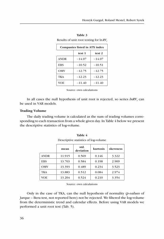
The values of lag k are selected upon information criteria AIC and BIC. Table 3 presents the results of testing.
36
Henryk Gurgul, Roland Mestel, Robert Syrek
table 3
Results of unit root testing for ln RVt
companies listed in AtX index
test 1 test 2
ANDR -14.07 -14.07
EBS -10.52 -10.51
OMV -12.75 -12.75
TKA -12.23 -12.23
VOE -11.40 -11.40
Source: own calculations
In all cases the null hypothesis of unit root is rejected, so series lnRVt can be used in VAR models.
trading Volume
The daily trading volume is calculated as the sum of trading volumes corre-sponding to each transaction from a whole given day. In Table 4 below we present the descriptive statistics of log-volume.
table 4
Descriptive statistics of log-volume
meanstd.
deviationkurtosis skewness
ANDR 11.915 0.569 0.146 3.322
EBS 13.703 0.584 0.198 2.909
OMV 13.393 0.489 0.234 3.523
TKA 13.883 0.512 0.084 2.974
VOE 13.204 0.524 0.210 3.354
Source: own calculations
Only in the case of TKA, can the null hypothesis of normality (p-values of Jarque – Bera test, not reported here) not be rejected. We filtered the log-volume from the deterministic trend and calendar effects. Before using VAR models we performed a unit root test (Tab. 5).
37
The Testing of Causal Stock Returns-Trading Volume Dependencies...
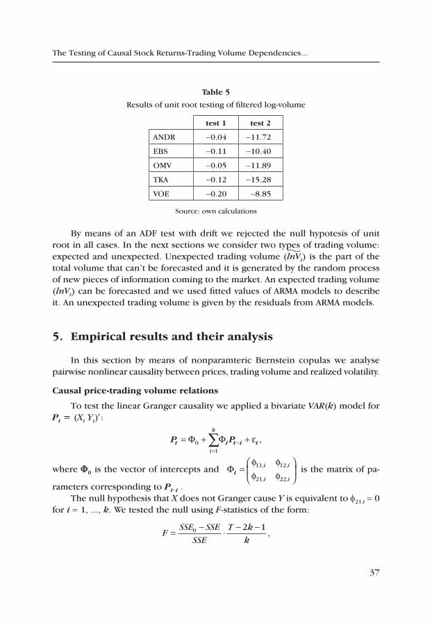
table 5
Results of unit root testing of filtered log-volume
test 1 test 2
ANDR -0.04 -11.72
EBS -0.11 -10.40
OMV -0.05 -11.89
TKA -0.12 -15.28
VOE -0.20 -8.85
Source: own calculations
By means of an ADF test with drift we rejected the null hypotesis of unit root in all cases. In the next sections we consider two types of trading volume: expected and unexpected. Unexpected trading volume (lnVt) is the part of the total volume that can’t be forecasted and it is generated by the random process of new pieces of information coming to the market. An expected trading volume (lnVt) can be forecasted and we used fitted values of ARMA models to describe it. An unexpected trading volume is given by the residuals from ARMA models.
5. empirical results and their analysis
In this section by means of nonparamteric Bernstein copulas we analyse pairwise nonlinear causality between prices, trading volume and realized volatility.
causal price‑trading volume relations
To test the linear Granger causality we applied a bivariate VAR(k) model for Pt = (Xt Yt)′:
P Pt i t i t= + +=
−∑F F01i
k
e ,
where F0 is the vector of intercepts and Fi =
f ff f
11 12
21 22
, ,
, ,
i i
i i
is the matrix of pa-
rameters corresponding to Pt-i .The null hypothesis that X does not Granger cause Y is equivalent to f21,i = 0
for i = 1, ..., k. We tested the null using F-statistics of the form:
FSSE SSE
SSET k
k= − ⋅ − −0 2 1
,
38
Henryk Gurgul, Roland Mestel, Robert Syrek
where SSE0 is the sum of the squared residuals of the restricted regression (f21,i = 0) and SSE is the sum of the squared residuals of the unrestricted model. The number of observations is denoted by T. Under the null the statistics pre-sented above is asymptotically F distributed with k and T - 2k - 1 the degrees of freedom. The choice of k is based on the AIC and the BIC criteria. The proper number k of time lags guarantees that residuals are uncorrelated.
In order to test the nonlinear causality we used the BRT statistics described in the previous section, applied to residuals from VAR models. Using this method we can be sure that we tested only nonlinear relations. When estimating the Bern-stein copulas we took the bandwidth k as the integer part of 2 T . We computed the p-values of the test with 200 bootstrap samples. Below we used the notations XY in order to describe the null hypothesis: X does not Granger cause Y.
realized volatility and expected trading volume
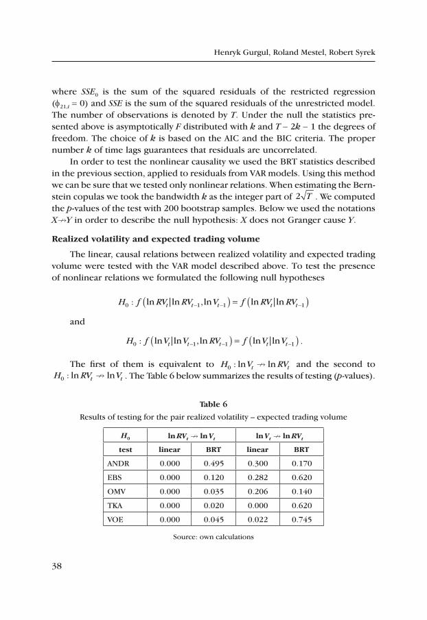
The linear, causal relations between realized volatility and expected trading volume were tested with the VAR model described above. To test the presence of nonlinear relations we formulated the following null hypotheses
H f RV RV V f RV RVt t t t t0 1 1 1: ln ln ,ln ln ln| |− − −( ) = ( )and
H f V V RV f V Vt t t t t0 1 1 1: ln ln ,ln ln ln| |− − −( ) = ( ) .
The first of them is equivalent to H V RVt t0 : ln ln and the second to H RV Vt t0 : ln ln . The Table 6 below summarizes the results of testing (p-values).
table 6
Results of testing for the pair realized volatility – expected trading volume
H0 ln RVt ln Vt ln Vt ln RVt
test linear Brt linear Brt
ANDR 0.000 0.495 0.300 0.170
EBS 0.000 0.120 0.282 0.620
OMV 0.000 0.035 0.206 0.140
TKA 0.000 0.020 0.000 0.620
VOE 0.000 0.045 0.022 0.745
Source: own calculations
39
The Testing of Causal Stock Returns-Trading Volume Dependencies...
In all cases there is linear causality running from realized volatility to expected trading volume. Causality in the opposite direction is detected only in the case of TKA and VOE. In addition, there is nonlinear causality running from lnRVt to lnVt for three stocks (OMV, TKA and VOE).
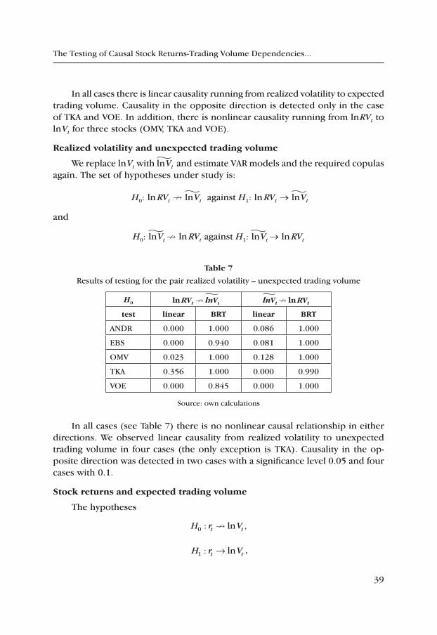
realized volatility and unexpected trading volume
We replace lnVt with lnVt and estimate VAR models and the required copulas again. The set of hypotheses under study is:
H0: ln RVt lnVt against H1: ln RVt → lnVt
and
H0: lnVt ln RVt against H1: lnVt → ln RVt
table 7
Results of testing for the pair realized volatility – unexpected trading volume
H0 ln RVt lnVt lnVt ln RVt
test linear Brt linear Brt
ANDR 0.000 1.000 0.086 1.000
EBS 0.000 0.940 0.081 1.000
OMV 0.023 1.000 0.128 1.000
TKA 0.356 1.000 0.000 0.990
VOE 0.000 0.845 0.000 1.000
Source: own calculations
In all cases (see Table 7) there is no nonlinear causal relationship in either directions. We observed linear causality from realized volatility to unexpected trading volume in four cases (the only exception is TKA). Causality in the op-posite direction was detected in two cases with a significance level 0.05 and four cases with 0.1.
Stock returns and expected trading volume
The hypotheses
H r Vt t0 : ln ,
H r Vt t1 : ln→ ,
40
Henryk Gurgul, Roland Mestel, Robert Syrek
in terms of conditional densities are formulated as follows:
H f V V r f V Vt t t t t0 1 1 1: ln ln , ln ln ,| |− − −( ) = ( )
H f V V r f V Vt t t t t1 1 1 1: ln ln , ln ln .| |− − −( ) ≠ ( )
The opposite direction of causal dependency has the form:
H f r r V f r rt t t t t0 1 1 1: , ,ln| |− − −( ) = ( )
H f r r V f r rt t t t t1 1 1 1: , ,ln .| |− − −( ) ≠ ( ) ,
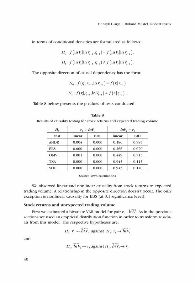
Table 8 below presents the p-values of tests conducted.
table 8
Results of causality testing for stock returns and expected trading volume
H0 rt lnVt lnVt rt
test linear Brt linear Brt
ANDR 0.004 0.000 0.186 0.985
EBS 0.000 0.000 0.266 0.070
OMV 0.001 0.000 0.449 0.715
TKA 0.000 0.000 0.945 0.115
VOE 0.000 0.000 0.945 0.140
Source: own calculations
We observed linear and nonlinear causality from stock returns to expected trading volume. A relationship in the opposite direction doesn’t occur. The only exception is nonlinear causality for EBS (at 0.1 significance level).
Stock returns and unexpected trading volume
First we estimated a bivariate VAR model for pair rt - lnVt. As in the previous sections we used an empricial distribution function in order to transform residu-als from this model. The respective hypotheses are:
H0: rt lnVt against H1: rt → lnVt
and
H0: lnVt rt against H1: lnVt → rt
41
The Testing of Causal Stock Returns-Trading Volume Dependencies...
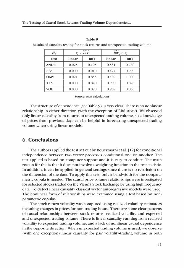
table 9
Results of causality testing for stock returns and unexpected trading volume
H0 rt lnVt lnVt rt
test linear Brt linear Brt
ANDR 0.025 0.105 0.531 0.760
EBS 0.000 0.010 0.474 0.990
OMV 0.021 0.855 0.402 1.000
TKA 0.000 0.840 0.909 0.820
VOE 0.000 0.890 0.909 0.865
Source: own calculations
The structure of dependence (see Table 9) is very clear. There is no nonlinear relationship in either direction (with the exception of EBS stock). We observed only linear causality from returns to unexpected trading volume, so a knowledge of prices from previous days can be helpful in forecasting unexpected trading volume when using linear models.
6. conclusions
The authors applied the test set out by Bouezmarni et al. [12] for conditional independence between two vector processes conditional one on another. The test applied is based on computer support and it is easy to conduct. The main reason for this is that it does not involve a weighting function in the test statistic. In addition, it can be applied in general settings since there is no restriction on the dimension of the data. To apply this test, only a bandwidth for the nonpara-metric copula is needed. The causal price-volume relationships were investigated for selected stocks traded on the Vienna Stock Exchange by using high frequency data. To detect linear causality classical vector autoregressive models were used. The nonlinear form of relationships were examined using a test based on non-parametric copulas.
The stock return volatility was computed using realized volatility estimators including changes in prices for non-trading hours. There are some clear patterns of causal relationships between stock returns, realized volatility and expected and unexpected trading volume. There is linear causality running from realized volatility to expected trading volume, and a lack of nonlinear causal dependence in the opposite direction. When unexpected trading volume is used, we observe (with one exception) linear causality for pair volatility-trading volume in both
42
Henryk Gurgul, Roland Mestel, Robert Syrek
directions and a lack of nonlinear causality. When regarding the pair stock returns and trading volume the conclusions depend on the part of trading volume used. There is a strong a linear and nonlinear causality from stock returns to expected trading volume, and a lack of such a relationship in the opposite direction. So a knowledge of past stock returns can improve forecasts of expected trading vol-ume. When regarding unexpected trading volume, we conclude that there is only a linear, causal relationship from stock returns to unexpected trading volume. Neither linear nor nonlinear causal relations from unexpected trading volume to stock returns are detected.
references
[1] Abhyankar A., Linear and non-linear Granger causality: Evidence from the U.K. stock index futures market, ”Journal of Futures Markets” 1998, vol. 18, pp. 519–540.
[2] Asimakopoulos I., Ayling D., Mahmood W.M., Non-linear Granger causality in the currency futures returns, “Economics Letters” 2000, vol. 68, pp. 25–30.
[3] Bandi F.M., Russell J.R., Separating microstructure noise from volatility, “Journal of Financial Economics” 2006, vol. 79(3), pp. 655–692.
[4] Bandi F.M., Russell J.R., Microstructure noise, realized variance, and optimal sampling, “Review of Economic Studies” 2008a, vol. 75(2), pp. 339–369.
[5] Bandi F.M., Russell J.R., Yang C., Realized volatility forecasting and option pricing, “Journal of Econometrics” 2008b, vol. 147(1), pp. 34–46.
[6] Bandi F.M., Russell J.R., Market microstructure noise, integrated variance estimators, and the accuracy of asymptotic approximations, “Journal of Econometrics” 2011, vol. 160(1), pp. 145–159.
[7] Baek E., Brock W., A general test for Granger causality: Bivariate model, Technical Report 1992, Iowa State University and University of Wisconsin, Madison.
[8] Barndorff-Nielsen O.E., Hansen P.R., Lunde A., Shephard N., Regular and modified kernel-based estimators of integrated variance: The case with independent noise?, “Economics Papers” 2004-W28, Economics Group, Nuffield College, University of Oxford.
[9] Barndorff-Nielsen O.E., Hansen P.R., Lunde A., Shephard N., Designing real-ized kernels to measure the ex-post variation of equity prices in the presence of noise, “Econometrica” 2008 , vol. 76(6), pp. 1481–1536.
[10] Barndorff-Nielsen O.E., Hansen P.R., Lunde A., Shephard N., Realized ker-nels in practice: Trades and quotes, “Econometrics Journal” 2009, vol. 12, pp. 1–32.
[11] Bollerslev T., Jubinski D., Equity trading volume volatility: latent informa-tion arrivals and common long-run dependencies, “Journal of Business & Economic Statistics” 1999, vol. 17, pp. 9–21.
43
The Testing of Causal Stock Returns-Trading Volume Dependencies...
[12] Bouezmarni T., Rombouts J.V.K., Taamouti A., A nonparametric copula based test for conditional independence with applications to Granger causality, “Journal of Business and Economic Statistics” 2012, to appear.
[13] Clark P.K., A subordinated stochastic process model with finite variance for speculative prices, “Econometrica“ 1973, vol. 41, pp. 135–156.
[14] Copeland T.E., A model of asset trading under the assumption of sequential information arrival, “Journal of Finance” 1976, vol. 31, pp. 1149–1168.
[15] Diks C., Panchenko V., A Note on the Hiemstra-Jones Test for Granger Non-causality, “Studies in Nonlinear Dynamics & Econometrics” 2005, vol. 9(2), Article 4.
[16] Diks C., Panchenko V., A new statistic and practical guidelines for non-parametric Granger causality testing, “Journal of Economic Dynamics and Control”, vol. 30(9–10), pp. 1647–1669.
[17] Epps T.W., Epps M.L., The stochastic dependence of security price changes and transaction volumes: implications for the mixture-of-distribution hy-pothesis, “Econometrica” 1976, vol. 44, pp. 305–321.
[18] Fleming J., Kirby C., Long memory in volatility and trading volume, “Journal of Banking & Finance” 2011, vol. 35(7), pp. 1714–1726.
[19] Gervais S., Kaniel R., Mingelgrin D., The high-volume return premium, “The Journal of Finance” 2001, vol. 56, pp. 877–919.
[20] Granger C.W.J., Investigating causal relations by econometric models and cross-spectral methods, “Econometrica” 1969, vol. 37 (3), pp. 424–438.
[21] Granger C.W.J., Newbold P., Spurious regression in econometrics, “Journal of Econometrics” 1974, vol. 2, pp. 111–120.
[22] Gurgul H., Lach Ł., Liniowa i nieliniowa przyczynowość dla spółek z indeksu DAX, „Badania Operacyjne i Decyzje” 2009, vol. 3, pp. 27–46.
[23] Gurgul H., Majdosz P., Mestel R., Price – volume relations of DAX companies, “Financial Markets and Portfolio Management” 2007, vol. 21, pp. 353–379.
[24] Gurgul H., Majdosz P., Mestel R., Joint Dynamics of Prices and Trading Volume on the Polish Stock Market, “Managing Global Transitions” 2005, vol. 3(2), pp. 139–156.
[25] Gurgul H., Wójtowicz T., Stopy zwrotu a wielkość obrotów na GPW w Warsza-wie, “Folia Oeconomica Cracoviensia” 2008, vol. 49–50, pp. 31–45.
[26] Hansen P.R., Lunde A., A realized variance for the whole day based on in-termittent high-frequency data, “Journal of Financial Econometrics” 2005, vol. 3(4), pp. 525–554.
[27] Hansen P.R., Lunde A., Realized variance and market microstructure noise, “Journal of Business and Economic Statistics” 2006, vol. 24(2), pp. 127–161.
[28] Harris L., Cross-security tests of the mixture of distributions hypothesis, “Journal of Financial and Quantitative Analysis” 1986, vol. 21, pp. 39–46.
[29] Hiemstra C., Jones J.D., Testing for linear and nonlinear Granger causality in the stock price – volume relation, “Journal of Finance” 1994, vol. 49, pp. 1639–1664.

Henryk Gurgul, Roland Mestel, Robert Syrek
[30] Karpoff J.M., The Relation between Price Changes and Trading Volume: A Survey, “Journal of Financial and Quantitative Analysis” 1987, vol. 22, pp. 109–126.
[31] Lee B.S., Rui O.M., The dynamic relationship between stock returns and trading volume: Domestic and cross-country evidence, “Journal of Banking and Finance” 2002, vol. 26, pp. 51–78.
[32] Linton O., Gozalo P., Conditional Independence Restrictions: Testing and Estimation, Discussion Paper 1997, Cowles Foundation for Research in Economics, Yale University.
[33] Luu J.C., Martens M., Testing the mixture-of-distributions hypothesis using “re-alized” volatility, “Journal of Futures Markets” 2003, vol. 23(7), pp. 661–679.
[34] McAleer M., Medeiros M., Realized volatility: A review, “Econometric Re-views” 2008, vol. 27, pp. 10–45.
[35] Nielsen M.Ø., Shimotsu K., Determining the cointegrating rank in nonsta-tionary fractional systems by the exact local Whittle approach, “Journal of Econometrics” 2007, vol. 141, pp. 574–96.
[36] Oomen R.C.A., Properties of realized variance under alternative sampling schemes, “Journal of Business and Economic Statistics” 2006, vol. 24, pp. 219–237.
[37] Paparoditis E., Politis D., The Local Bootstrap for Kernel Estimators under General Dependence Conditions, “Annals of the Institute of Statistical Math-ematics” 2000, vol. 52, pp. 139–159.
[38] Phillips C.P., Understanding the spurious regression in econometrics, “Journal o f Econometrics” 1986, vol. 33, pp. 311–40.
[39] Robinson P.M., Yajima Y., Determination of cointegrating rank in fractional systems, “Journal of Econometrics” 2002, vol. 106 (2), pp. 217–241.
[40] Rossi, E., de Magistris P.S., Long memory and tail dependence in trading volume and volatility, “CREATES Research Paper” No. 2009-30.
[41] Sims C.A., Stock J.H., Watson M.W., Inference in linear time series models with some unit roots, “Econometrica” 1990, vol. 58, pp. 133–144.
[42] Su L., White H., Testing Conditional Independence via Empirical Likelihood, Discussion Paper 2003, University of California San Diego.
[43] Su L., White H., A nonparametric Hellinger Metric test for Conditional Independence, ”Econometric Theory” 2008, vol. 24, pp. 1–36.
[44] Tauchen G.E.; Pitts M., The price variability – volume relationship on specu-lative markets, “Econometrica” 1983, vol. 51, pp. 485–505.
[45] Toda H.Y., Yamamoto T., Statistical inference in vector autoregressions with possibly integrated processes, “Journal of Econometrics” 1995, vol. 66, pp. 225–250.
[46] Zhang L., Mykland P., Aït-Sahalia Y., A tale of two time scales: determining integrated volatility with noisy high-frequency data, “Journal of the Ameri-can Statistical Association” 2005, vol. 100, pp. 1394–1411.
45
Managerial Economics2013, No. 13, pp. 45–64
http://dx.doi.org/10.7494/manage.2013.13.45
Henryk Gurgul*, Artur Machno*, Roland Mestel**
Modeling of returns and trading Volume by regime Switching copulas
1. introduction
The relations among international stock markets have been investigated in many papers, especially in the periods of financial crises. The topic under study is important for market participants because due to globalization process the global markets are becoming more and more dependent. This observation follows from liberalization and deregulation in money and capital markets. In addition, the globalization process diminishes opportunities for international diversification.
The financial data show asymmetric dependence. This feature is reflected in the observation that in the bear phase stock market data such as returns, trading volume and volatility are getting to be more dependent than in the bull stock market. This means that investors might lose advantages of international portfolios and these portfolios may be more risky than what the investors assume. The occur-rence of such asymmetric interdependence is also probable between returns and trading volume. The goal of this article is to describe co-movements of realized volatility and trading volume for selected stocks listed on Vienna Stock Exchange.
The remainder of the contribution is organized in the following way: in sec-tion 2 we conduct the literature overview concerning the dependence concepts, including regime switching models and copulas and discuss the recent contribu-tions to the subject; in section 3 we present the data; in the following section the dependence measures and copulas are overviewed; in the fifth section copula regime switching model is described; in the sixth section the results are reported and evaluated; section 7 concludes the paper.
* AGH University of Science and Technology in Cracow, Department of Applications of Mathematics in Economics, e–mails: [email protected]; [email protected]
Financial support for this paper from the National Science Centre of Poland (Research Grant DEC-2012/05/B/HS4/00810) is gratefully acknowledged.
** University of Applied Sciences Joanneum in Graz, Department of Banking and Insurance, e-mail: [email protected]

46
Henryk Gurgul, Artur Machno, Roland Mestel
2. Literature overview
The dependence between the stock markets can be measured through such variables as stock return, trading volume and volatility. The most frequently used methodology in the investigations of the interdependencies is based on Granger causality and VAR model (see [18]). In one of the earliest contributions on de-pendency of stock markets Eun and Shim ([15]) checked the relationships among nine major stock markets including Australia, Canada, France, Germany, Hong Kong, Japan, Switzerland, the UK and the US by means of the Vector Autoregressive (VAR) Model. The authors found that news in the US market has a major impact on the other markets. Lin et al.([31]) focused on interdependence between the returns and volatility of Japan and the US market indices using high frequency data of daytime and overnight returns. They established that daytime returns in the US or Japan market were linked with the overnight returns in the other.
Kim and Rogers ([27]) studied the dynamic interdependence between the stock markets of Korea, Japan, and the US. They underlined the importance of Japanese and the US stock markets for Korean market since the last became more open for foreign investors. By mean of EGARCH model Booth et al. ([11]) found strong interdependence among the Danish, Finnish, Norwegian and Swedish Stock Market. According to the authors the essential dependence started with the so-called Thailand currency crisis. However, it was not observed after the Hong Kong crisis. Ng ([33]) established significant causality running from the US and Japan stock market to six Asian markets: Hong Kong, Korea, Malaysia, Singapore, Taiwan and Thailand. Klein et al. ([28]) by means of wavelets technique, applied to three developed markets: US, Germany and Japan and two emerging markets Egypt and Turkey proved that changes in these developed markets had effects on the emerging markets. In the paper [6], using the VAR-EGARCH model, it is checked the interdependence among three EU markets namely Germany, France and the UK. The results supported the hypothesis of the cointegration among the mentioned stock markets.
Sharkasi et al. ([42]) used wavelet analysis and found the global co-movements among seven stock markets, three in Europe (Irish, UK, and Portuguese), two in the Americas (namely US, and Brazilian) and two in Asia (Japanese and Hong Kong).
The contributions by Ammermann and Patterson ([2]), Lim et al. (30), Lim and Hinich ([29]), Bessler et al. ([7]) or Bonilla et al. ([10]) tried to established a different pattern of the stock price development. The authors detected long random walk phases. They alternated with short ones and showed significant linear and/or nonlinear correlations. The contributors thought that these serial dependencies had an episodic character. Due to these contributors the serial de-pendencies caused the low performance of the forecasting models. Nivet ([34])
47
Modeling of Returns and Trading Volume by Regime Switching Copulas
checked the random walk hypothesis for the Warsaw Stock Exchange. Worthing-ton and Higgs ([46]) proved the efficiency on the Hungarian, Polish, Czech and Russian stock markets. The Hungarian stock market followed the random walk. Gilmore and McManus ([17]) found autocorrelations in some of the Central and Eastern European stock markets. Schotman and Zalewska ([43]), claimed that the nonsynchronous trading and asymmetric response to good and bad news were reason for autocorrelation.
Todea et al. ([45]) applied the Hinich–Patterson windowed-test procedure. By means of it, he investigated the temporal persistence of linear and, especially, non-linear interdependencies among six Central and Eastern European stock markets.
Issues concerning asymmetry of dependence, were analyzed by Longin and Solnik ([32]). The contributors found (by means of the constant conditional correlation (CCC) model introduced by Bollerslev ([8]) that the correlations be-tween the stock markets over a period of three decades were not stable over this time period. In addition, they increased during more volatile periods. Moreover, they depended on some economic variables such as interest rates, buybacks or dividend yields. Some results based on extreme value theory were showed in Ang and Chen ([5]). The authors derived a test for asymmetric correlation. They suggested comparison of empirical and model-based conditional correlations. The authors justified that regime switching models were most suitable for modelling of asymmetry. Ang and Bekaert in [3] and [4] applied a Gaussian Markov switch-ing model for international returns. They estimated two regimes: a bull regime with positive mean, low volatilities and low correlations; and a bear regime with negative returns, high volatilities and correlation.
Regime switching models were introduced in econometrics by Hamilton ([21]). Currently they found many applications in finance. In the papers [19] and [20] is being concerned the interest rate, the methodology of regime switching models was used. The contributors used also a regime switching model for inter-national financial returns. In the paper ([31]) the regime switching modelling was applied to the model correlation. The author assumed a normal distribution. The marginals were modelled with the GARCH. The model by Pelletier was something “intermediate” between the constant conditional correlation (CCC) of Bollerslev ([8]) and the dynamic conditional correlation (DCC) model of Engle ([14]).
Patton ([36]) indicated a significant asymmetry in the structure of dependence of the financial returns what is very important for a certain kind of investors. In his further contributions (see [37] and [38]), he introduced conditional copulas and time-varying models of bivariate dependence of coefficients in order to model foreign exchange rates. Jondeau and Rockinger ([26]) applied the skewed-t GARCH models for returns with univariate time-varying skewness. Finally, in order to measure the dependence between pairs of countries, they used a time-varying or
48
Henryk Gurgul, Artur Machno, Roland Mestel
a switching Gaussian, or Student t copula. Jondeau and Rockinger ([26]) and Hu ([25]) suggested the so-called copula based multivariate dynamic (CMD) model. Klein at al. ([28]) conducted an extensive simulation study, and demonstrated that CMD models were proper tools for investigating different time series with the GARCH structure for the squared residuals. They showed that the copula (mis-) specification should play a key role before the usage of the CMD model.
In recent years the economists combined copulas and regime switching models in bivariate financial data. Rodriguez ([41]) and Okimoto ([35]) applied regime switching copulas for pairs of international stock indices. While Okimoto ([35]) dealt with the US-UK pair, Rodriguez ([41]) worked with pairs of Latin American and Asian countries. The contributors applied methodology developed by Ramchand and Susmel ([40]) with a structure where variances, means and correlations switched together in the two-variable system. Garcia and Tsafak ([16]) estimated a regime switching model in a four-variable system of domestic and foreign stocks and bonds. The authors used a mixture of bivariate copulas to model the dependence between all possible pairs of variables.
Chollete et al. ([12]) generalized the Pelletier ([39]) model to the non-Gauss-ian case. The authors excluded the Gaussian assumption, because the returns were not Gaussian and suggested a regime switching structure for dependence. They used flexible multivariate copulas. They also tried to separate the asymmetry in the marginals from the one in the dependence. This could not have been done in a Gaussian switching model. Their investigations were based on copulas. The authors instead of Gaussian marginal distribution applied the skewed t GARCH model of Hansen ([24]).
The authors applied their model in multivariate case and therefore they made their approach more appropriate for practical applications. They used the canonical vine copula, which allowed very general types of dependence.
The authors found that the VaR and Expected Shortfall of the canonical vine models were essentially better than the Student t or Gaussian copula models, which implied that the inappropriate usage of the latter models could lead to the underestimation of the risk of a portfolio.
In order to model the observed asymmetric dependence in pairs trading volume realized volatility, we estimated a bivariate copula based on a regime switching model. We applied this model to high frequency data from Vienna Stock Exchange. The choice of copula is important for the risk management, be-cause it modifies the Value at Risk (VaR) and Expected Shortfall of international portfolio returns. We will check the dynamics of the interdependence between realized volatility and trading volume. The main goal is to document changes in the dependency and the asymmetry in both quiet and hectic (bull or bear) phase in the stock markets.
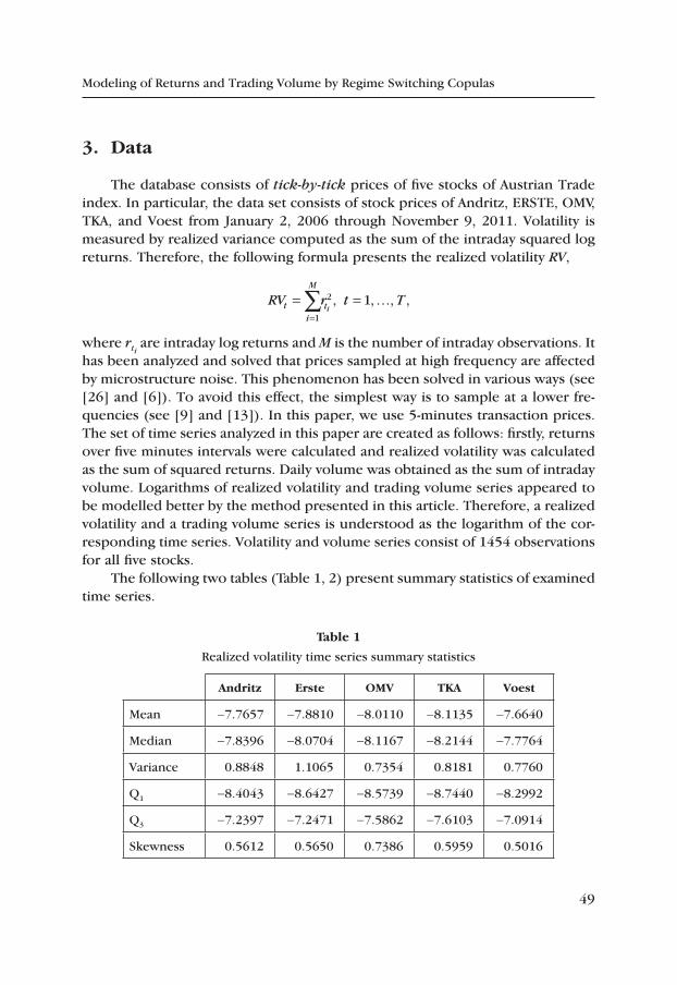
49
Modeling of Returns and Trading Volume by Regime Switching Copulas
3. Data
The database consists of tick-by-tick prices of five stocks of Austrian Trade index. In particular, the data set consists of stock prices of Andritz, ERSTE, OMV, TKA, and Voest from January 2, 2006 through November 9, 2011. Volatility is measured by realized variance computed as the sum of the intraday squared log returns. Therefore, the following formula presents the realized volatility RV,
RV r t Tti
M
ti= = …
=∑
1
2 1, , , ,
where rti are intraday log returns and M is the number of intraday observations. It
has been analyzed and solved that prices sampled at high frequency are affected by microstructure noise. This phenomenon has been solved in various ways (see [26] and [6]). To avoid this effect, the simplest way is to sample at a lower fre-quencies (see [9] and [13]). In this paper, we use 5-minutes transaction prices. The set of time series analyzed in this paper are created as follows: firstly, returns over five minutes intervals were calculated and realized volatility was calculated as the sum of squared returns. Daily volume was obtained as the sum of intraday volume. Logarithms of realized volatility and trading volume series appeared to be modelled better by the method presented in this article. Therefore, a realized volatility and a trading volume series is understood as the logarithm of the cor-responding time series. Volatility and volume series consist of 1454 observations for all five stocks.
The following two tables (Table 1, 2) present summary statistics of examined time series.
table 1
Realized volatility time series summary statistics
Andritz erste OMV tKA Voest
Mean -7.7657 -7.8810 -8.0110 -8.1135 -7.6640
Median -7.8396 -8.0704 -8.1167 -8.2144 -7.7764
Variance 0.8848 1.1065 0.7354 0.8181 0.7760
Q1 -8.4043 -8.6427 -8.5739 -8.7440 -8.2992
Q3 -7.2397 -7.2471 -7.5862 -7.6103 -7.0914
Skewness 0.5612 0.5650 0.7386 0.5959 0.5016
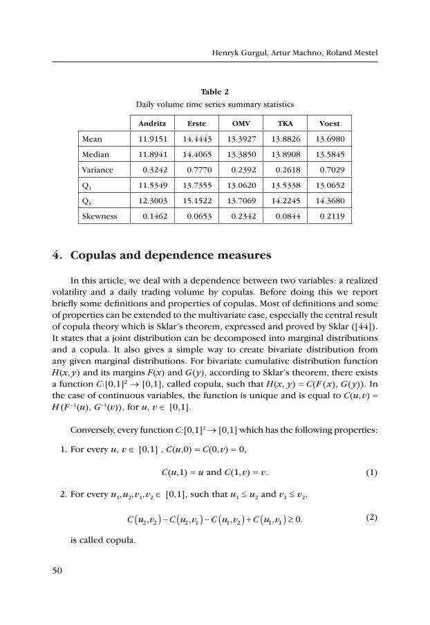
50
Henryk Gurgul, Artur Machno, Roland Mestel
table 2
Daily volume time series summary statistics
Andritz erste OMV tKA Voest
Mean 11.9151 14.4443 13.3927 13.8826 13.6980
Median 11.8941 14.4065 13.3850 13.8908 13.5845
Variance 0.3242 0.7770 0.2392 0.2618 0.7029
Q1 11.5349 13.7355 13.0620 13.5338 13.0652
Q3 12.3003 15.1522 13.7069 14.2245 14.3680
Skewness 0.1462 0.0653 0.2342 0.0844 0.2119
4. copulas and dependence measures
In this article, we deal with a dependence between two variables: a realized volatility and a daily trading volume by copulas. Before doing this we report briefly some definitions and properties of copulas. Most of definitions and some of properties can be extended to the multivariate case, especially the central result of copula theory which is Sklar’s theorem, expressed and proved by Sklar ([44]). It states that a joint distribution can be decomposed into marginal distributions and a copula. It also gives a simple way to create bivariate distribution from any given marginal distributions. For bivariate cumulative distribution function H(x, y) and its margins F(x) and G(y), according to Sklar’s theorem, there exists a function C:[0,1]2 → [0,1], called copula, such that H(x, y) = C(F (x), G(y)). In the case of continuous variables, the function is unique and is equal to C(u,v) = H(F -1(u), G-1(v)), for u, v ∈ [0,1].
Conversely, every function C:[0,1]2 → [0,1] which has the following properties:
1. For every u, v ∈ [0,1] , C(u,0) = C(0,v) = 0,
C(u,1) = u and C(1,v) = v. (1)
2. For every u1,u2,v1,v2 ∈ [0,1], such that u1 ≤ u2 and v1 ≤ v2,
C u v C u v C u v C u v2 2 2 1 1 2 1 1 0, , , , .( ) − ( ) − ( ) + ( ) ≥ (2)
is called copula.

51
Modeling of Returns and Trading Volume by Regime Switching Copulas
Those two concepts of copula function are in fact equivalent. Every copula obtained from Sklar’s theorem satisfies (1) and (2). Conversely, if C:[0,1]2 → [0,1] satisfies (1) and (2), there exists a pair of variables X and Y for which C is the copula obtained from Sklar’s theorem. Clearly, a copula can be considered as the cumulative distribution function of the bivariate random variable with uniformly distributed margins. According to this, for given copula C, we denote its density function as c. Therefore, for continuous random variables X and Y:
h x y f x g y c F x G y, , ,( ) = ( ) ( ) ( ) ( )( )where h(x, y) is joint density function of random vector (X, Y); f(x) and g(y) are density functions and F(x) and F(y) are cumulative distribution functions of X and Y, respectively.
The simplest copula is P(u, v) = uv. It connects independent margins. Other interesting examples are, so called, Fréchet-Hoeffding copula bounds, for u, v in [0,1]. They are defined by:
W u v u v M u v u v, max{ , }, , min{ , }.( ) = + − ( ) =1 0
The generalization of the function W to higher dimensions is not a copula. Only in two dimensions it is a copula, in which case it corresponds to counter-monotonic random variables.
The function W and M are called lower and upper Fréchet-Hoeffding copula bounds, because for any copula C and u, v in [0,1], we have:
W u v C u v M u v, , , .( ) ≤ ( ) ≤ ( )
Copulas used in this article are the Gaussian copula and two-parameter Ar-chimedean copulas BB1, BB4 and BB7. The Gaussian copula is constructed from a bivariate normal distribution. For given correlation r, the Gaussian copula with parameter r can be written as
C u vGaussr = ( ) ( )( )− −F F FS
1 1, , (3)
where F-1 is the inverse cumulative distribution function of the standard normal distribution and FS is the joint cumulative distribution function of a bivariate
normal distribution with mean zero and covariance matrix S =
1
1
rr
.
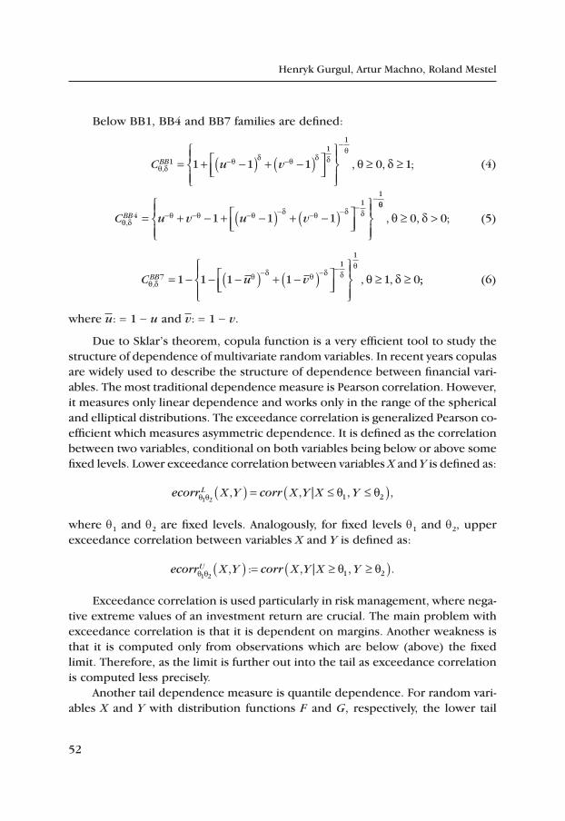
52
Henryk Gurgul, Artur Machno, Roland Mestel
Below BB1, BB4 and BB7 families are defined:
C u vBBq d
q d q d dq
q d, , , ;1
11
1 1 1 0 1= + −( ) + −( )
≥ ≥− −
−
(4)
C u v u vBBq d
q q q d q d d,
4
11
1 1 1= + − + −( ) + −( )
− − − − − − −
q d, , ;≥ >0 0 (5)
C u vBBq d
q d q d dq
q d, , ,7
11
1 1 1 1 1 0= − − −( ) + −( )
≥ ≥
− − −;; (6)
where u: = 1 - u and v: = 1 - v.
Due to Sklar’s theorem, copula function is a very efficient tool to study the structure of dependence of multivariate random variables. In recent years copulas are widely used to describe the structure of dependence between financial vari-ables. The most traditional dependence measure is Pearson correlation. However, it measures only linear dependence and works only in the range of the spherical and elliptical distributions. The exceedance correlation is generalized Pearson co-efficient which measures asymmetric dependence. It is defined as the correlation between two variables, conditional on both variables being below or above some fixed levels. Lower exceedance correlation between variables X and Y is defined as:
ecorr X Y corr X Y X YLq q q q1 2 1 2, , , ,( ) = ≤ ≤( )|
where θ1 and θ2 are fixed levels. Analogously, for fixed levels θ1 and θ2, upper exceedance correlation between variables X and Y is defined as:
ecorr X Y corr X Y X YUq q q q1 2 1 2, : , , .( ) = ≥ ≥( )|
Exceedance correlation is used particularly in risk management, where nega-tive extreme values of an investment return are crucial. The main problem with exceedance correlation is that it is dependent on margins. Another weakness is that it is computed only from observations which are below (above) the fixed limit. Therefore, as the limit is further out into the tail as exceedance correlation is computed less precisely.
Another tail dependence measure is quantile dependence. For random vari-ables X and Y with distribution functions F and G, respectively, the lower tail
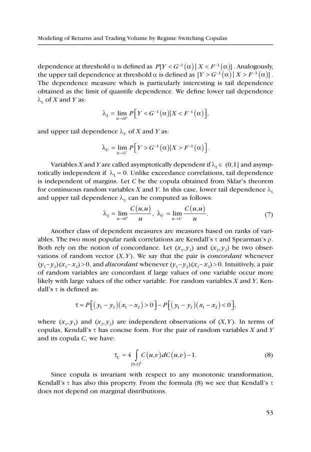
53
Modeling of Returns and Trading Volume by Regime Switching Copulas
dependence at threshold a is defined as P Y G X F[ | ]< ( ) < ( )− −1 1a a . Analogously, the upper tail dependence at threshold a is defined as [ | ]Y G X F> ( ) > ( )− −1 1a a . The dependence measure which is particularly interesting is tail dependence obtained as the limit of quantile dependence. We define lower tail dependence lL of X and Y as:
l a aa
L P Y G X F= < ( ) < ( ) →− −
+lim ,
0
1 1|
and upper tail dependence lU of X and Y as:
l a aa
U P Y G X F= > ( ) > ( ) →− −
−lim .
1
1 1|
Variables X and Y are called asymptotically dependent if lL ∈ (0,1] and asymp-totically independent if lL = 0. Unlike exceedance correlations, tail dependence is independent of margins. Let C be the copula obtained from Sklar’s theorem for continuous random variables X and Y. In this case, lower tail dependence lL and upper tail dependence lU can be computed as follows:
l lLu
Uu
C u u
u
C u u
u=
( )=
( )→ →+ −lim
,, lim
,.
0 1 (7)
Another class of dependent measures are measures based on ranks of vari-ables. The two most popular rank correlations are Kendall’s t and Spearman’s r. Both rely on the notion of concordance. Let (x1, y1) and (x2, y2) be two obser-vations of random vector (X, Y). We say that the pair is concordant whenever (y1-y2)(x1- x2)> 0, and discordant whenever (y1-y2)(x1- x2)> 0. Intuitively, a pair of random variables are concordant if large values of one variable occur more likely with large values of the other variable. For random variables X and Y, Ken-dall’s t is defined as:
t = −( ) −( ) > − −( ) −( ) < P y y x x P y y x x1 2 1 2 1 2 1 20 0 ,
where (x1, y1) and (x2, y2) are independent observations of (X, Y). In terms of copulas, Kendall’s t has concise form. For the pair of random variables X and Y and its copula C, we have:
tC C u v dC u v= ( ) ( ) −∫4 10 1 2[ , ]
, , . (8)
Since copula is invariant with respect to any monotonic transformation, Kendall’s t has also this property. From the formula (8) we see that Kendall’s t does not depend on marginal distributions.
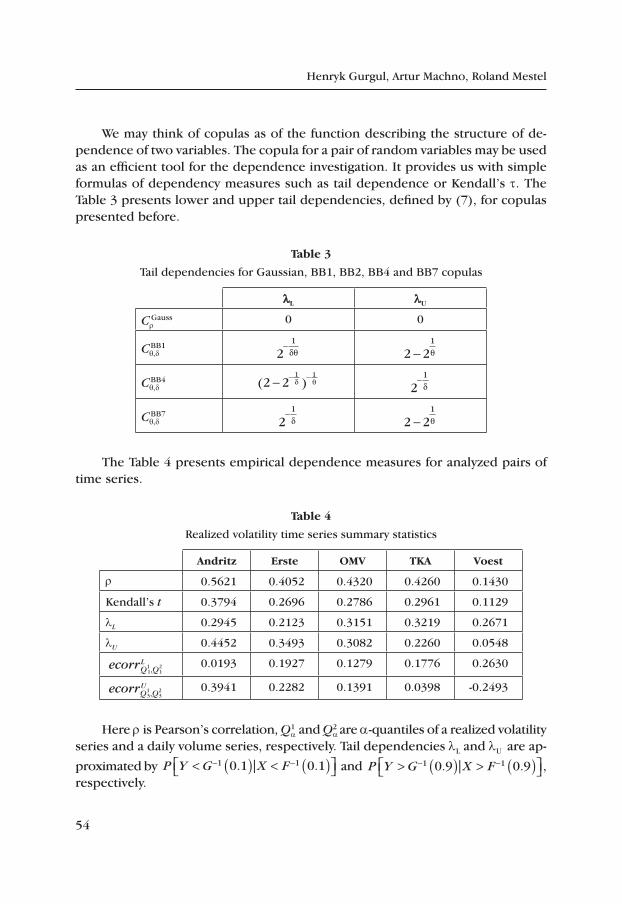
54
Henryk Gurgul, Artur Machno, Roland Mestel
We may think of copulas as of the function describing the structure of de-pendence of two variables. The copula for a pair of random variables may be used as an efficient tool for the dependence investigation. It provides us with simple formulas of dependency measures such as tail dependence or Kendall’s t. The Table 3 presents lower and upper tail dependencies, defined by (7), for copulas presented before.
table 3
Tail dependencies for Gaussian, BB1, BB2, BB4 and BB7 copulas
lL lU
CrGauss 0 0
Cθ,dBB1
21−dq 2 2
1
− q
Cθ,dBB4 ( )2 2
1 1− − −d q 2
1−d
Cθ,dBB7
21−d 2 2
1
− q
The Table 4 presents empirical dependence measures for analyzed pairs of time series.
table 4
Realized volatility time series summary statistics
Andritz erste OMV tKA Voest
r 0.5621 0.4052 0.4320 0.4260 0.1430
Kendall’s t 0.3794 0.2696 0.2786 0.2961 0.1129
lL 0.2945 0.2123 0.3151 0.3219 0.2671
lU 0.4452 0.3493 0.3082 0.2260 0.0548
ecorrLQ1
1,Q21
0.0193 0.1927 0.1279 0.1776 0.2630
ecorrUQ1
3,Q23
0.3941 0.2282 0.1391 0.0398 -0.2493
Here r is Pearson’s correlation, Q1a and Q2
a are a-quantiles of a realized volatility series and a daily volume series, respectively. Tail dependencies lL and lU are ap-
proximated by P Y G X F< ( ) < ( ) − −1 10 1 0 1. .| and P Y G X F> ( ) > ( )
− −1 10 9 0 9. .| , respectively.
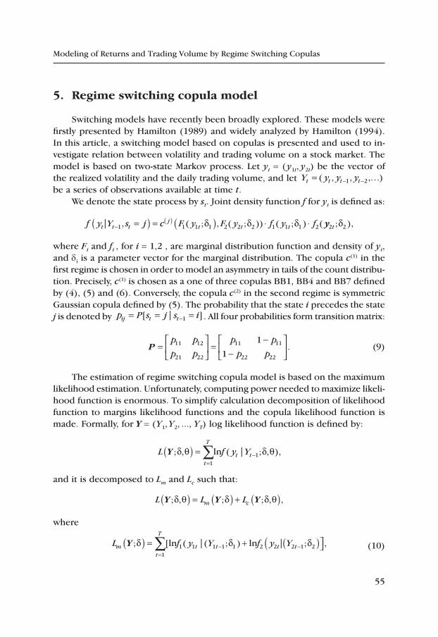
55
Modeling of Returns and Trading Volume by Regime Switching Copulas
5. regime switching copula model
Switching models have recently been broadly explored. These models were firstly presented by Hamilton (1989) and widely analyzed by Hamilton (1994). In this article, a switching model based on copulas is presented and used to in-vestigate relation between volatility and trading volume on a stock market. The model is based on two-state Markov process. Let yt = (y1t, y2t) be the vector of the realized volatility and the daily trading volume, and let Y y y yt t t t= …− −( , , , )1 2 be a series of observations available at time t.
We denote the state process by st. Joint density function f for yt is defined as:
f y Y s j c F y F y f y ft t tj
t t t| −( )=( ) = ( ) ⋅ ⋅1 1 1 1 2 2 2 1 1 1 2, ( ; , ( ; )) ( ; ) (d d d yy t2 2; ),d
where Fi and fi , for i = 1,2 , are marginal distribution function and density of yi, and di is a parameter vector for the marginal distribution. The copula c(1) in the first regime is chosen in order to model an asymmetry in tails of the count distribu-tion. Precisely, c(1) is chosen as a one of three copulas BB1, BB4 and BB7 defined by (4), (5) and (6). Conversely, the copula c(2) in the second regime is symmetric Gaussian copula defined by (5). The probability that the state i precedes the state j is denoted by p P s j s iij t t= = =−[ | ]1 . All four probabilities form transition matrix:
P =
=
−−
p p
p p
p p
p p11 12
21 22
11 11
22 22
1
1. (9)
The estimation of regime switching copula model is based on the maximum likelihood estimation. Unfortunately, computing power needed to maximize likeli-hood function is enormous. To simplify calculation decomposition of likelihood function to margins likelihood functions and the copula likelihood function is made. Formally, for Y = (Y1, Y2, ..., YT) log likelihood function is defined by:
L f y Yt
T
t tY ; , ( | ; , ),d q d q( ) ==
−∑1
1ln
and it is decomposed to Lm and Lc such that:
L L Lm cY Y Y; , ; ; , ,d q d d q( ) = ( ) + ( )
where
L f y Y f y Ymt
T
t t t tY ; [ ( |( ; ) ; ,d d d( ) = + ( )( =
− −∑1
1 1 1 1 1 2 2 2 1 2ln ln | (10)
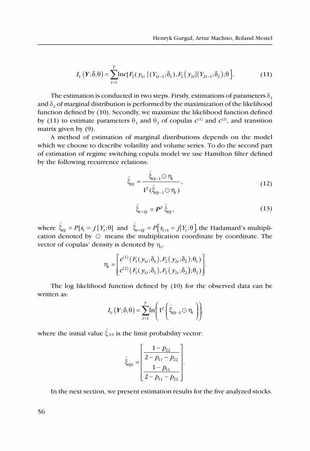
56
Henryk Gurgul, Artur Machno, Roland Mestel
L c F y Y F y Yct
T
t t t tY ; , [ ( |( ; ), ; ;d q d d q( ) = ( )( =
− −∑1
2 1 1 1 1 2 2 2 1 2ln | .. (11)
The estimation is conducted in two steps. Firstly, estimations of parameters d1 and d2 of marginal distribution is performed by the maximization of the likelihood function defined by (10). Secondly, we maximize the likelihood function defined by (11) to estimate parameters θ1 and θ2 of copulas c(1) and c(2), and transition matrix given by (9).
A method of estimation of marginal distributions depends on the model which we choose to describe volatility and volume series. To do the second part of estimation of regime switching copula model we use Hamilton filter defined by the following recurrence relations:
xx h
x h
^^
^||
|( ),t t
t t t
Tt t t
= −
−
1
11
(12)
x x^ ^
| | ,t tT
t t+ =1 P (13)
where x q^
| [ | ; ]t t t tP s j Y= = and x q^
| ; ,t t t tP s j Y+ += = 1 1 | the Hadamard’s multipli-cation denoted by means the multiplication coordinate by coordinate. The vector of copulas’ density is denoted by ht,
h
d d q
d dtt t
t t
c F y F y
c F y F y=
( ) ( )( ) (
( )
( )
11 1 1 2 2 2 1
21 1 1 2 2 2
( ; , ; ; )
( ; , ; ))
; ).
q2
The log likelihood function defined by (10) for the observed data can be written as:
Lct
TT
t t tY ; , ,^
|d q x h( ) =
=−∑
111ln
where the initial value x^1|0 is the limit probability vector:
x^
| .1 0
22
11 22
11
11 22
12
12
=
−−
−−
−
−
pp p
pp p
In the next section, we present estimation results for the five analyzed stocks.
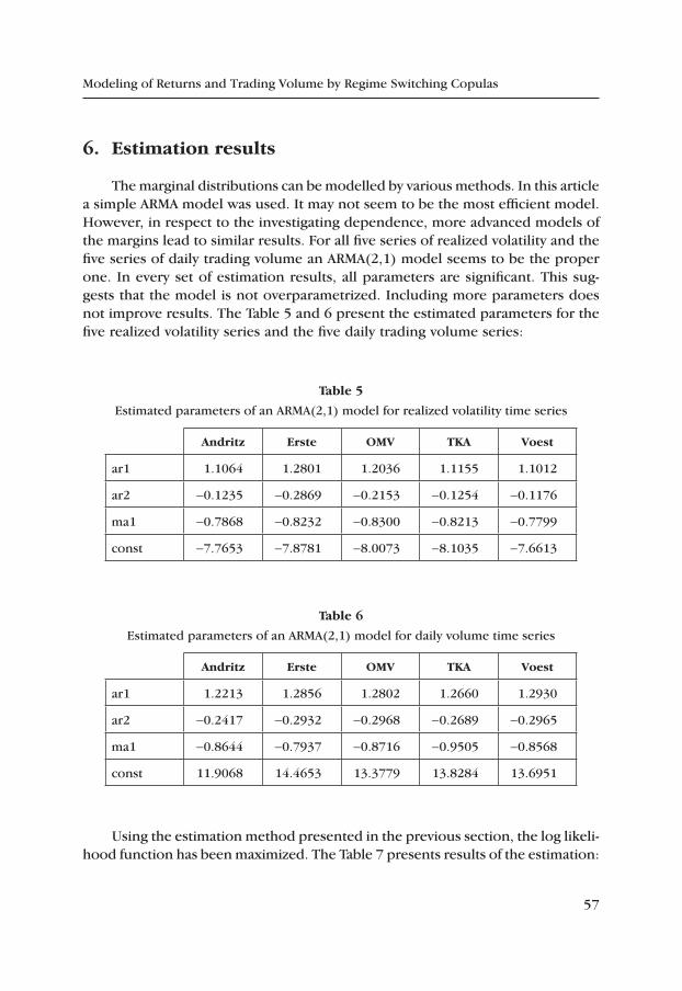
57
Modeling of Returns and Trading Volume by Regime Switching Copulas
6. estimation results
The marginal distributions can be modelled by various methods. In this article a simple ARMA model was used. It may not seem to be the most efficient model. However, in respect to the investigating dependence, more advanced models of the margins lead to similar results. For all five series of realized volatility and the five series of daily trading volume an ARMA(2,1) model seems to be the proper one. In every set of estimation results, all parameters are significant. This sug-gests that the model is not overparametrized. Including more parameters does not improve results. The Table 5 and 6 present the estimated parameters for the five realized volatility series and the five daily trading volume series:
table 5
Estimated parameters of an ARMA(2,1) model for realized volatility time series
Andritz erste OMV tKA Voest
ar1 1.1064 1.2801 1.2036 1.1155 1.1012
ar2 -0.1235 -0.2869 -0.2153 -0.1254 -0.1176
ma1 -0.7868 -0.8232 -0.8300 -0.8213 -0.7799
const -7.7653 -7.8781 -8.0073 -8.1035 -7.6613
table 6
Estimated parameters of an ARMA(2,1) model for daily volume time series
Andritz erste OMV tKA Voest
ar1 1.2213 1.2856 1.2802 1.2660 1.2930
ar2 -0.2417 -0.2932 -0.2968 -0.2689 -0.2965
ma1 -0.8644 -0.7937 -0.8716 -0.9505 -0.8568
const 11.9068 14.4653 13.3779 13.8284 13.6951
Using the estimation method presented in the previous section, the log likeli-hood function has been maximized. The Table 7 presents results of the estimation:
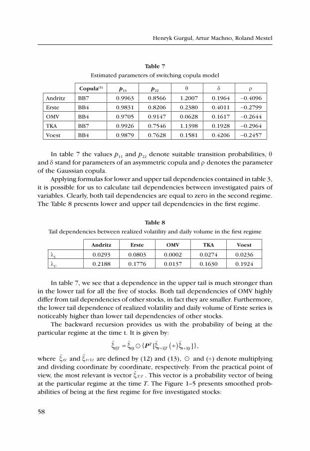
58
Henryk Gurgul, Artur Machno, Roland Mestel
table 7
Estimated parameters of switching copula model
copula(1) p11 p22 θ d r
Andritz BB7 0.9963 0.8566 1.2007 0.1964 -0.4096
Erste BB4 0.9831 0.8206 0.2380 0.4011 -0.2799
OMV BB4 0.9705 0.9147 0.0628 0.1617 -0.2644
TKA BB7 0.9926 0.7546 1.1398 0.1928 -0.2964
Voest BB4 0.9879 0.7628 0.1581 0.4206 -0.2457
In table 7 the values p11 and p22 denote suitable transition probabilities, θ and d stand for parameters of an asymmetric copula and r denotes the parameter of the Gaussian copula.
Applying formulas for lower and upper tail dependencies contained in table 3, it is possible for us to calculate tail dependencies between investigated pairs of variables. Clearly, both tail dependencies are equal to zero in the second regime. The Table 8 presents lower and upper tail dependencies in the first regime.
table 8
Tail dependencies between realized volatility and daily volume in the first regime
Andritz erste OMV tKA Voest
lL 0.0293 0.0803 0.0002 0.0274 0.0236
lU 0.2188 0.1776 0.0137 0.1630 0.1924
In table 7, we see that a dependence in the upper tail is much stronger than in the lower tail for all the five of stocks. Both tail dependencies of OMV highly differ from tail dependencies of other stocks, in fact they are smaller. Furthermore, the lower tail dependence of realized volatility and daily volume of Erste series is noticeably higher than lower tail dependencies of other stocks.
The backward recursion provides us with the probability of being at the particular regime at the time t. It is given by:
x x x x^ ^ ^ ^
| | | |{ ,[ ]}t T t tT
t T t t= ÷( )+ + P 1 1
where x^t|t and x^t+1|t are defined by (12) and (13), and (÷) denote multiplying and dividing coordinate by coordinate, respectively. From the practical point of view, the most relevant is vector x^T |T . This vector is a probability vector of being at the particular regime at the time T. The Figure 1–5 presents smoothed prob-abilities of being at the first regime for five investigated stocks:
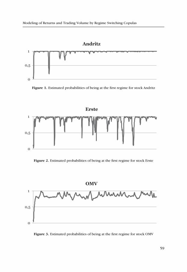
59
Modeling of Returns and Trading Volume by Regime Switching Copulas
Figure 1. Estimated probabilities of being at the first regime for stock Andritz
Figure 2. Estimated probabilities of being at the first regime for stock Erste
Figure 3. Estimated probabilities of being at the first regime for stock OMV
0
0,5
1
Andritz
0
0,5
1
Erste
0
0,5
1
OMV
0
0,5
1
Andritz
0
0,5
1
Erste
0
0,5
1
OMV
0
0,5
1
Andritz
0
0,5
1
Erste
0
0,5
1
OMV
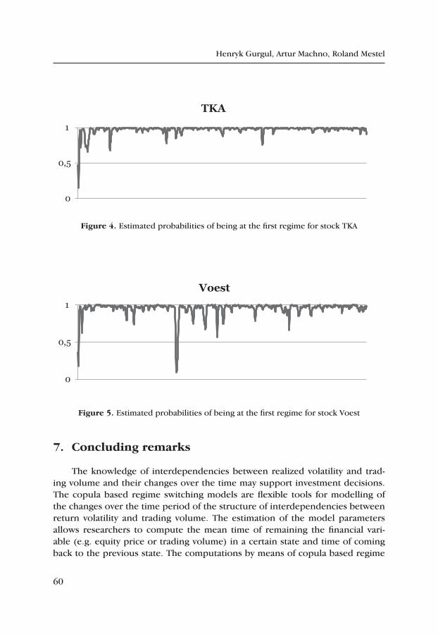
60
Henryk Gurgul, Artur Machno, Roland Mestel
Figure 4. Estimated probabilities of being at the first regime for stock TKA
Figure 5. Estimated probabilities of being at the first regime for stock Voest
7. concluding remarks
The knowledge of interdependencies between realized volatility and trad-ing volume and their changes over the time may support investment decisions. The copula based regime switching models are flexible tools for modelling of the changes over the time period of the structure of interdependencies between return volatility and trading volume. The estimation of the model parameters allows researchers to compute the mean time of remaining the financial vari-able (e.g. equity price or trading volume) in a certain state and time of coming back to the previous state. The computations by means of copula based regime
0
0,5
1
TKA
0
0,5
1
Voest
0
0,5
1
TKA
0
0,5
1
Voest
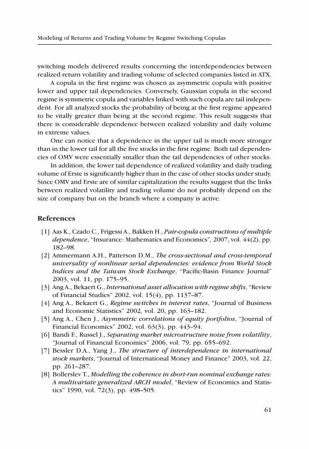
61
Modeling of Returns and Trading Volume by Regime Switching Copulas
switching models delivered results concerning the interdependencies between realized return volatility and trading volume of selected companies listed in ATX.
A copula in the first regime was chosen as asymmetric copula with positive lower and upper tail dependencies. Conversely, Gaussian copula in the second regime is symmetric copula and variables linked with such copula are tail indepen-dent. For all analyzed stocks the probability of being at the first regime appeared to be vitally greater than being at the second regime. This result suggests that there is considerable dependence between realized volatility and daily volume in extreme values.
One can notice that a dependence in the upper tail is much more stronger than in the lower tail for all the five stocks in the first regime. Both tail dependen-cies of OMV were essentially smaller than the tail dependencies of other stocks.
In addition, the lower tail dependence of realized volatility and daily trading volume of Erste is significantly higher than in the case of other stocks under study. Since OMV and Erste are of similar capitalization the results suggest that the links between realized volatility and trading volume do not probably depend on the size of company but on the branch where a company is active.
references
[1] Aas K., Czado C., Frigessi A., Bakken H., Pair-copula constructions of multiple dependence, “Insurance: Mathematics and Economics”, 2007, vol. 44(2), pp. 182–98.
[2] Ammermann A.H., Patterson D.M., The cross-sectional and cross-temporal universality of nonlinear serial dependencies: evidence from World Stock Indices and the Taiwan Stock Exchange, “Pacific-Basin Finance Journal” 2003, vol. 11, pp. 175–95.
[3] Ang A., Bekaert G., International asset allocation with regime shifts, “Review of Financial Studies” 2002, vol. 15(4), pp. 1137–87.
[4] Ang A., Bekaert G., Regime switches in interest rates, “Journal of Business and Economic Statistics” 2002, vol. 20, pp. 163–182.
[5] Ang A., Chen J., Asymmetric correlations of equity portfolios, “Journal of Financial Economics” 2002, vol. 63(3), pp. 443–94.
[6] Bandi F., Russel J., Separating market microstructure noise from volatility, “Journal of Financial Economics” 2006, vol. 79, pp. 655–692.
[7] Bessler D.A., Yang J., The structure of interdependence in international stock markets, “Journal of International Money and Finance” 2003, vol. 22, pp. 261–287.
[8] Bollerslev T., Modelling the coherence in short-run nominal exchange rates: A multivariate generalized ARCH model, “Review of Economics and Statis-tics” 1990, vol. 72(3), pp. 498–505.
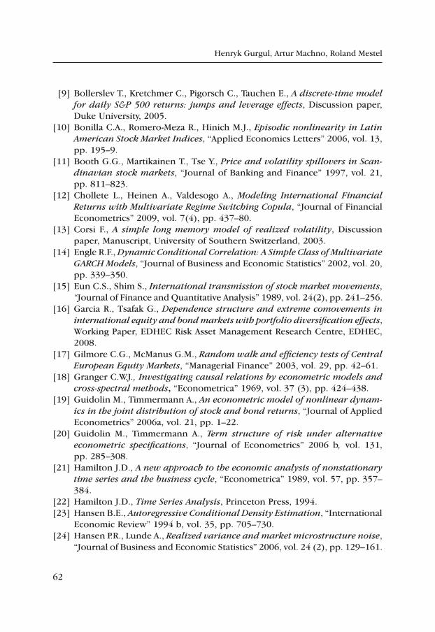
62
Henryk Gurgul, Artur Machno, Roland Mestel
[9] Bollerslev T., Kretchmer C., Pigorsch C., Tauchen E., A discrete-time model for daily S&P 500 returns: jumps and leverage effects, Discussion paper, Duke University, 2005.
[10] Bonilla C.A., Romero-Meza R., Hinich M.J., Episodic nonlinearity in Latin American Stock Market Indices, “Applied Economics Letters” 2006, vol. 13, pp. 195–9.
[11] Booth G.G., Martikainen T., Tse Y., Price and volatility spillovers in Scan-dinavian stock markets, “Journal of Banking and Finance” 1997, vol. 21, pp. 811–823.
[12] Chollete L., Heinen A., Valdesogo A., Modeling International Financial Returns with Multivariate Regime Switching Copula, “Journal of Financial Econometrics” 2009, vol. 7(4), pp. 437–80.
[13] Corsi F., A simple long memory model of realized volatility, Discussion paper, Manuscript, University of Southern Switzerland, 2003.
[14] Engle R.F., Dynamic Conditional Correlation: A Simple Class of Multivariate GARCH Models, “Journal of Business and Economic Statistics” 2002, vol. 20, pp. 339–350.
[15] Eun C.S., Shim S., International transmission of stock market movements, “Journal of Finance and Quantitative Analysis” 1989, vol. 24(2), pp. 241–256.
[16] Garcia R., Tsafak G., Dependence structure and extreme comovements in international equity and bond markets with portfolio diversification effects, Working Paper, EDHEC Risk Asset Management Research Centre, EDHEC, 2008.
[17] Gilmore C.G., McManus G.M., Random walk and efficiency tests of Central European Equity Markets, “Managerial Finance” 2003, vol. 29, pp. 42–61.
[18] Granger C.W.J., Investigating causal relations by econometric models and cross-spectral methods, “Econometrica” 1969, vol. 37 (3), pp. 424–438.
[19] Guidolin M., Timmermann A., An econometric model of nonlinear dynam-ics in the joint distribution of stock and bond returns, “Journal of Applied Econometrics” 2006a, vol. 21, pp. 1–22.
[20] Guidolin M., Timmermann A., Term structure of risk under alternative econometric specifications, “Journal of Econometrics” 2006 b, vol. 131, pp. 285–308.
[21] Hamilton J.D., A new approach to the economic analysis of nonstationary time series and the business cycle, “Econometrica” 1989, vol. 57, pp. 357–384.
[22] Hamilton J.D., Time Series Analysis, Princeton Press, 1994.[23] Hansen B.E., Autoregressive Conditional Density Estimation, “International
Economic Review” 1994 b, vol. 35, pp. 705–730.[24] Hansen P.R., Lunde A., Realized variance and market microstructure noise,
“Journal of Business and Economic Statistics” 2006, vol. 24 (2), pp. 129–161.
63
Modeling of Returns and Trading Volume by Regime Switching Copulas
[25] Hu L., Dependence Patterns Across Financial Markets, “Applied Financial Economics” 2006, vol. 16, pp. 717–729.
[26] Jondeau E., Rockinger M., The Copula-GARCH Model of Conditional Depen-dences: An International Stock Market Application, “Journal of International Money and Finance” 2006, vol. 25(5), pp. 27–53.
[27] Kim S.W., Rogers J.H., International stock price spillovers and market lib-eralization: Evidence from Korea, Japan, and the United States, “Journal of Empirical Finance” 1995, vol. 2, pp. 117–133.
[28] Klein I., Köck C., Tinkl F., Spatial-serial dependency in multivariate GARCH models and dynamic copulas: a simulation study, „Ekonomia Menedżerska” 2010, no 7, pp. 43–62.
[29] Lim K.P., Hinich M.J., Cross-temporal universality of nonlinear dependencies in Asian Stock Markets, “Economics Bulletin” 2005, vol. 7, pp. 1–6.
[30] Lim K.P., Hinich M.J., Liew K.S., Episodic non-linearity and non-stationarity in ASEAN exchange rates returns series, “Labuan Bulletin of International Business and Finance” 2003, vol. 1, pp. 79–93.
[31] Lin W., Engle R., Ito T., Do bulls and bears move across borders?, Inter-national transmission of stock returns and volatility, “Review of Financial Studies” 1994, vol. 7(3), pp. 507–538.
[32] Longin F., Solnik B., Extreme Correlation of International Equity Markets, “Journal of Finance” 2001, vol. 56(2), pp. 649–76.
[33] Ng A., Volatility spillover effect from Japan and the US to the Pacific-Basin, “Journal of International Money and Finance” 2000, vol. 19, pp. 207–233.
[34] Nivet J.F., Stock markets in transition: the Warsaw experiment, “Economics of Transition” 1997, vol. 5, pp. 171–83.
[35] Okimoto T., New Evidence of Asymmetric Dependence Structures in Inter-national Equity Markets, “Journal of Financial and Quantitative Analysis” 2008, vol. 43(3), pp. 787–815.
[36] Patton A., On the out-of-sample importance of skewness and asymmetric dependence for asset allocation, “Journal of Financial Econometrics” 2004, vol. 2(1), pp. 130–168.
[37] Patton A., Estimation of multivariate models for time series of possibly different lengths, “Journal of Applied Econometrics” 2006a, vol. 21(2), pp. 147–173.
[38] Patton A., Modelling asymmetric exchange rate dependence, “International Economic Review” 2006b, vol. 47(2), pp. 527–556.
[39] Pelletier D., Regime switching for dynamic correlation, “Journal of Econo-metrics” 2006, vol. 131, pp. 445–473.
[40] Ramchand L., Susmel R., Volatility and cross correlation across major stock markets, “Journal of Empirical Finance” 1998, vol. 17, pp. 581–610.
[41] Rodriguez J., Measuring financial contagion: A copula approach, “Journal of Empirical Finance” 2007, vol. 14, pp. 401–423.

Henryk Gurgul, Artur Machno, Roland Mestel
[42] Sharkasi A., Ruskin H.J., Crane M., Interrelationships among international stock market indices: Europe, Asia and the Americas, “International Journal of Theoretical and Applied Finance” 2005, vol. 8(5), pp. 603–622.
[43] Schotman P.C., Zalewska A., Non-synchronous trading and testing for market integration in Central European emerging markets, “Journal of Empirical Finance” 2006, 13, pp. 462–494.
[44] Sklar A., Fonctions de répartition a n dimensions et leurs marge, Publications de l’Institut de Statistique de l’Universite de Paris, vol. 8, pp. 229–231.
[45] Todea A., Zaicas-Lenciu A., Episodic dependencies in Central and Eastern Europe stock markets, “Applied Economics Letters” 2008, vol. 15, pp. 1123– 1126.
[46] Worthington A.C., Higgs H., Random walks and market efficiency in Eu-ropean equity markets, “Global Journal of Finance and Economics” 2004, vol. 1, pp. 59–78.
65
Managerial Economics2013, No. 13, pp. 65–82
http://dx.doi.org/10.7494/manage.2013.13.65
Henryk Gurgul*, Marcin Suder*
Modeling of Withdrawals from Selected AtMs of the “euronet” Network
1. introduction
The financial sector in any country deals with large amounts of data on cus-tomers. This data is collected for use in the improvement of their services. The detection of tendencies and patterns of customer behavior reflected in the data is very important in respect for marketing, profit maximization and customer value management.
In particular a better understanding of consumer habits with respect to ATM withdrawals is crucial for the logistic management of this type of service and may assist in other studies on the topic. One of the most important tasks in the explo-ration of such data is to use it to manage risk by means of econometric models which are used for forecasts of the future behavior of customers.
This contribution is concerned with forecasts of the amounts of money that individuals withdraw from ATMs (automated teller machines). These forecasts may be useful in particular for ATM replenishment strategies.
Investigations focusing on payment systems have attracted scholarly atten-tion in recent decades. This area of research combine monetary economics and banking theory (Takala, and Viren [28]). However, data on ATM transactions is far from being fully explored. Databases on ATM transactions exhibit a large coverage and are dependent on time. The reason is that there is typically become available a delay in availability, usually a few days after the reference period. However, this information is at present not being taken into account by public statistical institu-tions like the Central Statistical Office in Poland.
It is hard to find in the financial literature advanced econometric models for ATM withdrawal amounts especially those taking into account calendar effects.
* AGH University of Science and Technology, Department of Applications of Mathematics in Economics e-mail: [email protected], [email protected]

66
Henryk Gurgul, Marcin Suder
In existing contributions used simple linear models are usual, which take into account typical features of ATM withdrawals like calendar effects or seasonality. Although more advanced models often fit the ATM data better, they are inappro-priate as forecasting tools. The reason is that estimation process of parameters of more complex models is time consuming process.
That is why in practice it is impossible to conduct fast forecasts by means of complex models in the case of thousands of ATMs. In these situations simple linear models may appear more desirable.
The new idea in this paper is the application of switch SARIMA models to ATM data. Since switch ARIMA models fit the data well, especially ex post fore-casts, one can expect good performance of this kind of model in the forecasting of ATM withdrawals (forecasts ex ante).
The remaining part of the paper is organized as follows. Section 2 presents a literature overview. The following section shows the data and a description of it. In the fourth section models applied are given. In the next section empirical results are cited. The sixth section concludes the paper.
2. Literature overview
Calendar effects are an important feature of much financial and economic data. In the light of the results on ATM withdrawals presented in previous papers by Gurgul and Suder [17], [18] seasonality and calendar effects are also exhibited by this kind of data. Therefore, the literature review and the models in the em-pirical part of this contribution are determined by the results reported in these papers. Calendar effects being taken into account by dummies and the SARIMA model, the fitting of the mixture of normal distributions and the use of Markov switching models were the main focus in these papers. The literature overview below refers mainly to contributions dealing with these issues.
Most economic time series are directly or indirectly reflected in daily activ-ity. They are usually recorded on a daily, monthly, quarterly basis or some other period. Thus, economic variables may be affected by daily calendar effects, which started to be noted in the late seventies e.g. Cleveland and Devlin [7] and Liu [22]. The number of working days and its link with seasonal effects are impor-tant examples. They can be considered as easily anticipated effects which affect the short-term movements of time series. These periodic fluctuations must be adequately detected and modeled in or der to better analyze other non-periodic properties (Young, [29]).
67
Modeling of Withdrawals from Selected ATMs of the “Euronet” Network
The correction for calendar and seasonal effects may help suit this informa-tion for use as input to improve the performance of short-term macroeconomic forecasts (see [15]), as a tool for now casting private consumption (see [9]) or as a timely indicator of retail trade statistics (see [6]).This is why analyses concern-ing economic developments are adjusted for seasonal and working day effects.
Besides the number of working days, the day of the week, the week of the month, other calendar effects such as public holidays or religious events may also affect time series. For the particular series under study, calendar effects are of particular importance given that cash withdrawals vary over time and are often overlaid with additional factors such as paydays, holidays and seasonal demand, and are subject to trends and generally follow weekly, monthly and annual cycles. This type of calendar effect is mentioned in papers such as Simutis et al. [26] and is related to the logistic management of the ATM system. Institutional Change in the Payments System is addressed by Schmitz and Wood (2006).
One of the earliest statistical analyses is that of credit card transactions published by Hand and Blunt [20]. In the financial literature there has been some interest in establishing the relationship between ATMs and the demand for cash. Amromin and Chakravorti [1] applied a linear regression and performed a panel data analysis in order to compare countries. The authors focused on the growth in debit card point-of-sale transactions. Boeschoten [3] and Snellman and Viren [27] pursued similar goals. However, they derived their conclusions on the basis of models of individual customer behavior. Boeschoten [3] investigated data from a survey of Dutch consumers between 1990 and 1994 by means of a deterministic inventory model. The authors assumed that individuals maintain a certain level of cash. It is used at a constant rate. They replenish their stock when it falls below a certain threshold. The contributors found that ATM users typically had a lower stock than non-users because the cost to them of obtaining cash was lower. The relationship between the cost of obtaining cash and the number of ATMs was modeled in Snellman and Viren [27] as a deterministic optimization problem, where costs were assumed to be proportional to distance from ATMs. Although these economic papers used models for customer with-drawal amounts and times, they involve simplifications to enable conclusions about macro demand for cash and can be improved when making predictions at an individual level.
Findley and Monsell [10] dealt with the necessity of taking into account different days of the week. Monthly activity can depend on the numbers of days in a particular month and the kinds of days. There can be a significant effect of the Easter season, since these holidays are mobile and scheduled from March to April. Therefore in some years these holidays are in the first quarter and some-
68
Henryk Gurgul, Marcin Suder
times in the second. Different calendar effects were studied in the contribution by Simutiset al. [26]in the context of ATM logistics.
According to Findley et al. [11] taking into account calendar effects is of great importance, because it improves the features of the respective time series and leads to better results in modeling.
The literature contains different methods for the detection, estimation and adjustment of the time series which exhibit calendar effects. Cleveland and Dev-lin [7], [8]established, on the basis of a large sample, a distribution of withdrawal frequencies for monthly time series. They found the main frequencies for these time series. Findley and Soukup [12], [13], [14] analysed the applicability of dis-tributions in samples in order to check the day effect. McElroy and Holland [23]suggested a nonparametric test for distribution of maxima in samples.
Withdrawals from ATMs exhibit seasonality patterns, which can be analysed by e.g. X-12-ARIMA and Tramo-Seats. This problem is complex because of mobile holidays like Easter, Ramadan or the Chinese New Year (see [19]).
Brentnall et al. [4] developed a random-effects point pro cess model for automated teller machine withdrawals. They discussed estimation, prediction and computational issues. The authors stressed that their model may be used to forecast the behavior of an individual and to assess when changes in the pat-tern of individual behavior have occurred and as a description of behavior for a portfolio of accounts.
In a more recent contribution Brentnall et al. [5] took a multinomial distribu-tion for the distribution of amounts and random effects were modeled by a Dirich-let distribution or the empirical distribution of individual maximum likelihood. The next model derived by the authors extended the multinomial distribution by incorporating a form of serial dependence and using an empirical distribution for random effects. The contributors, on the basis of a sample of 5000 UK high-street bank accounts, found that the greatest benefit from the models was for accounts with a small number of past transactions. They also found that a little information may be lost by binning and that the Dirichlet distribution might overestimate the probability of previously unobserved withdrawal amounts. The authors showed that the empirical distribution of random effects performed well because there were a large number of individual accounts.
Kufel [21]used two methods for the detection of seasonality: regression based on dummies and harmonic analysis. His results based on withdrawals time series for ATMs in Torun showed yearly, monthly, weekly and daily seasonality. The calendar effect is especially important in the case of daily withdrawals from an ATM, because this issue has not yet been dealt with sufficiently in the scientific literature (see [24]).
In the next section we will describe and conduct a preliminary analysis of the dataset properties.

69
Modeling of Withdrawals from Selected ATMs of the “Euronet” Network
3. Dataset and its properties
Our empirical analysis was based on a dataset containing daily withdrawals from 293 ATMs located in the province of Małopolska and Podkarpacie. For each ATM we examined time series covering a period no shorter than one year. In general, the dataset covers the period January 2008 – March 2012. We will also consider the issue of location when formulating final conclusions of this study. The number of examined ATMs with respect to their location are presented in Table 1:
table 1
The number of examined ATMs with respect to their location
Location Number
Bank Branch 84
Entertainment Centre 6
Supermarket 40
Hotel 6
Gas Station 25
Shop 49
Shopping Center 42
Transport 4
Other 37
Total 293
Source: own elaboration
The detailed results of empirical computations will be presented for four ATMs, which were chosen according to location criteria, i.e. each ATM has a dif-ferent location. In Table 2 a short description of the location and some basic descriptive statistics for the ATMs chosen are presented, while Figures 1–4 pres-ent the plots of time series of daily withdrawals from these ATMs. Examining ATMs from different locations may provide some help in answering the question whether the statistical properties of the time series of withdrawals depend on the type of location considered.
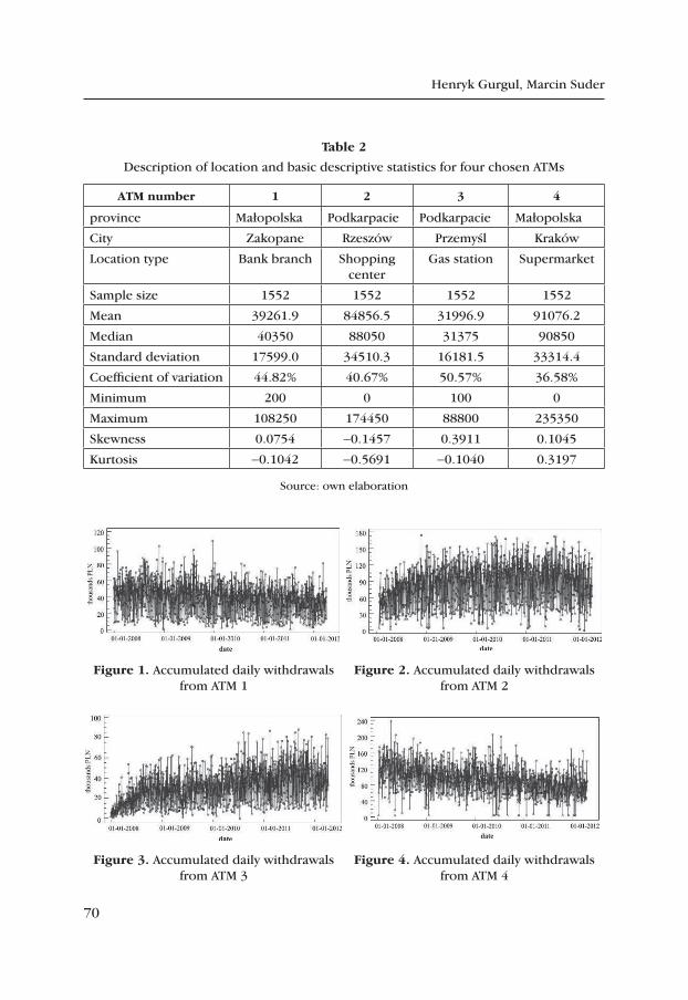
70
Henryk Gurgul, Marcin Suder
table 2
Description of location and basic descriptive statistics for four chosen ATMs
AtM number 1 2 3 4
province Małopolska Podkarpacie Podkarpacie Małopolska
City Zakopane Rzeszów Przemyśl Kraków
Location type Bank branch Shopping center
Gas station Supermarket
Sample size 1552 1552 1552 1552
Mean 39261.9 84856.5 31996.9 91076.2
Median 40350 88050 31375 90850
Standard deviation 17599.0 34510.3 16181.5 33314.4
Coefficient of variation 44.82% 40.67% 50.57% 36.58%
Minimum 200 0 100 0
Maximum 108250 174450 88800 235350
Skewness 0.0754 -0.1457 0.3911 0.1045
Kurtosis -0.1042 -0.5691 -0.1040 0.3197
Source: own elaboration
Figure 1. Accumulated daily withdrawals from ATM 1
Figure 2. Accumulated daily withdrawals from ATM 2
Figure 3. Accumulated daily withdrawals from ATM 3
Figure 4. Accumulated daily withdrawals from ATM 4
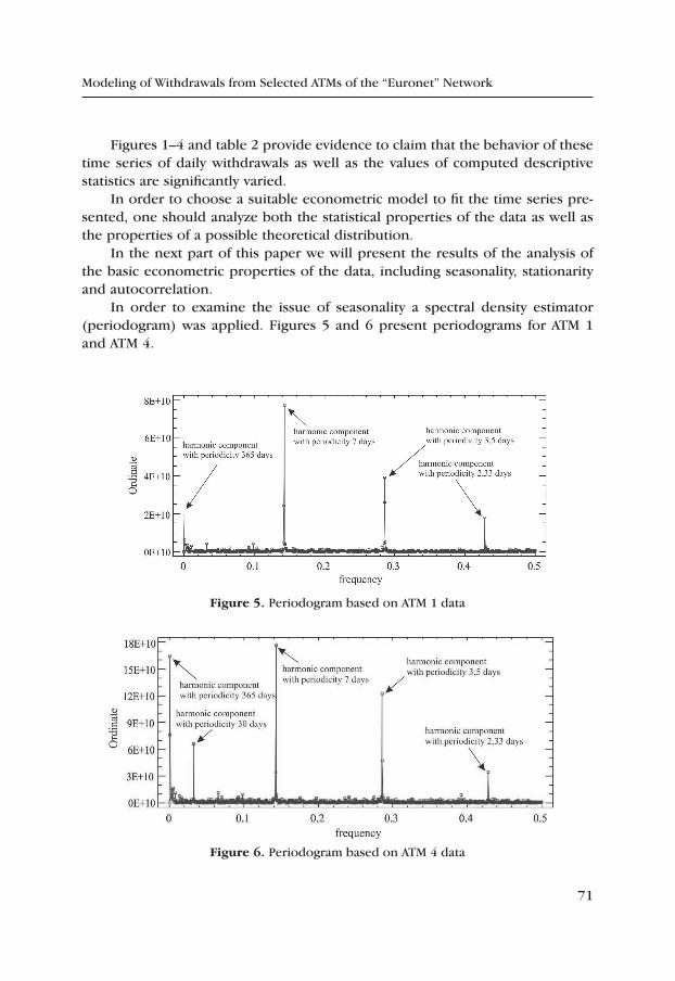
71
Modeling of Withdrawals from Selected ATMs of the “Euronet” Network
Figures 1–4 and table 2 provide evidence to claim that the behavior of these time series of daily withdrawals as well as the values of computed descriptive statistics are significantly varied.
In order to choose a suitable econometric model to fit the time series pre-sented, one should analyze both the statistical properties of the data as well as the properties of a possible theoretical distribution.
In the next part of this paper we will present the results of the analysis of the basic econometric properties of the data, including seasonality, stationarity and autocorrelation.
In order to examine the issue of seasonality a spectral density estimator (periodogram) was applied. Figures 5 and 6 present periodograms for ATM 1 and ATM 4.
Figure 5. Periodogram based on ATM 1 data
Figure 6. Periodogram based on ATM 4 data
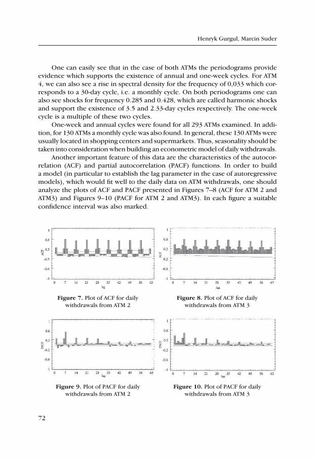
72
Henryk Gurgul, Marcin Suder
One can easily see that in the case of both ATMs the periodograms provide evidence which supports the existence of annual and one-week cycles. For ATM 4, we can also see a rise in spectral density for the frequency of 0,033 which cor-responds to a 30-day cycle, i.e. a monthly cycle. On both periodograms one can also see shocks for frequency 0.285 and 0.428, which are called harmonic shocks and support the existence of 3.5 and 2.33-day cycles respectively. The one-week cycle is a multiple of these two cycles.
One-week and annual cycles were found for all 293 ATMs examined. In addi-tion, for 130 ATMs a monthly cycle was also found. In general, these 130 ATMs were usually located in shopping centers and supermarkets. Thus, seasonality should be taken into consideration when building an econometric model of daily withdrawals.
Another important feature of this data are the characteristics of the autocor-relation (ACF) and partial autocorrelation (PACF) functions. In order to build a model (in particular to establish the lag parameter in the case of autoregressive models), which would fit well to the daily data on ATM withdrawals, one should analyze the plots of ACF and PACF presented in Figures 7–8 (ACF for ATM 2 and ATM3) and Figures 9–10 (PACF for ATM 2 and ATM3). In each figure a suitable confidence interval was also marked.
Figure 7. Plot of ACF for daily withdrawals from ATM 2
Figure 8. Plot of ACF for daily withdrawals from ATM 3
Figure 9. Plot of PACF for daily withdrawals from ATM 2
Figure 10. Plot of PACF for daily withdrawals from ATM 3
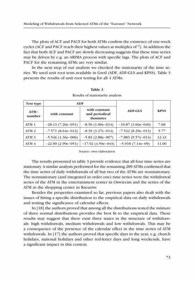
73
Modeling of Withdrawals from Selected ATMs of the “Euronet” Network
The plots of ACF and PACF for both ATMs confirm the existence of one-week cycles (ACF and PACF reach their highest values at multiples of 7). In addition the fact that both ACF and PACF are slowly decreasing suggests that these time series may be driven by e.g. an ARIMA process with specific lags. The plots of ACF and PACF for the remaining ATMs are very similar.
In the next step of our analysis we checked the stationarity of the time se-ries. We used unit root tests available in Gretl (ADF, ADF-GLS and KPSS). Table 3 presents the results of unit root testing for all 4 ATMs:
table 3
Results of stationarity analysis
test type ADF
ADF‑GLS KpSSAtM \number
with constantwith constant and periodical
dummies
ATM 1 -28.13 (7.26e-051) -8.56 (1.00e-014) -19.87 (3.66e-040) 7.68
ATM 2 -7.571 (8.64e-012) -8.39 (3.27e-014) -7.522 (8.29e-013) 5.77
ATM 3 -5.546 (1.36e-006) -5.83 (2.88e-007) -7.883 (9.57e-014) 12.43
ATM 4 -22.90 (2.99e-051) -17.92 (4.59e-043) -5.918 (7.14e-09) 11.00
Source: own elaboration
The results presented in table 3 provide evidence that all four time series are stationary. A similar analysis performed for the remaining 289 ATMs confirmed that the time series of daily withdrawals of all but two of the ATMs are nonstationary. The nonstationary (and integrated in order one) time series were the withdrawal series of the ATM in the entertainment center in Oswiecim and the series of the ATM in the shopping center in Rzeszów.
Besides the properties examined so far, previous papers also dealt with the issues of fitting a specific distribution to the empirical data on daily withdrawals and testing the significance of calendar effects.
In [18] the authors proved that among all the distributions tested the mixture of three normal distributions provides the best fit to the empirical data. These results may suggest that there exist three states in the structure of withdraw-als: high withdrawals, medium withdrawals and low withdrawals. This may be a consequence of the presence of the calendar effect in the time series of ATM withdrawals. In [17] the authors proved that specific days in the year, e.g. church holidays, national holidays and other red-letter days and long weekends, have a significant impact in this context.

74
Henryk Gurgul, Marcin Suder
The basic statistical and econometric analysis proved that although the time series are related to different locations, their basic properties are quite similar. Thus, one may claim that it is reasonable to use the same econometric model for the all time series under study. This would significantly simplify the procedure of building forecast models and support their practical applications.
4. Modeling of withdrawals from AtM
As mentioned in section 1, papers dealing with the issue of modeling ATM withdrawals are relatively rare, especially studies dealing with an analysis of a single ATM. Taking into account the properties of the dataset, the results presented in section 3, and the suggestions of [17] and [18], in this paper we applied a SARIMA model. This kind of model was, however, applied only to certain subseries, not the full time series available. Using the suggestions related to the issue of fitting a theoretical distribution to the empirical data which are presented in [18], from each time series two or three subseries were selected according to data division in the process of distribution fitting. For each of these subseries, an individual SARIMA model was estimated.
In addition, in this paper the results of analyzing traditional ARIMA and SARIMA models with dummy variables are also presented. Although these models are quite often used for forecasting purposes in time series analysis, their applica-tion in the case of the time series of daily withdrawals has not been described in the literature so far. Thus, it may turn out that these models provide a relatively good fit to the data, which could predispose them to various forecasting issues. On the other hand, if these models do not fit well to the empirical data it may suggest that some other directions should be followed in further research.
All examined models were estimated via maximum likelihood. The lag length was established based on information criteria, mainly the Akaike criterion. When this criterion reached similar values for different lag length, the mean absolute percentage error (MAPE) was compared in order to establish the final lag length. Moreover, for each model traditional diagnostic tests were conducted to test for the normality of distribution of the error term (Jarque–Bera test),the autocorrela-tion of the error term (Durbin-Watson test) and the presence of ARCH structures in the residuals (Engle ARCH test).
4.1. empirical results
In this section we present the empirical results obtained during the estimation of individual time series models. For each of the four ATMs examined, a detailed
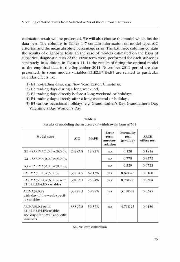
75
Modeling of Withdrawals from Selected ATMs of the “Euronet” Network
estimation result will be presented. We will also choose the model which fits the data best. The columns in Tables 4–7 contain information on model type, AIC criterion and the mean absolute percentage error. The last three columns contain the results of diagnostic tests. In the case of models estimated on the basis of subseries, diagnostic tests of the error term were performed for each subseries separately. In addition, in Figures 11–14 the results of fitting the optimal model to the empirical data in the September 2011–November 2011 period are also presented. In some models variables E1,E2,E3,E4,E5 are related to particular calendar effects like:
1) E1 no-trading days, e.g. New Year, Easter, Christmas, 2) E2 trading days during a long weekend, 3) E3 trading days directly before a long weekend or holidays, 4) E4 trading days directly after a long weekend or holidays, 5) E5 various occasional holidays, e.g. Grandmother’s Day, Grandfather’s Day,
Valentine’s Day, Women’s Day.
table 4
Results of modeling the structure of withdrawals from ATM 1
Model typeAic MApe
error term
autocor‑relation
Normality test
(p‑value)ArcH
effect test
G1 – SARIMA(1,0,0)x(0,0,0)7
G2 – SARIMA(0,0,0)x(5,0,0)7
G3 – SARIMA(2,0,0)x(0,0,0)7
24987.8 12.82% no 0.120 0.1814
no 0.778 0.4572
no 0.329 0.0723
SARIMA(1,0,0)x(5,0,0)7 33784.5 62.13% yes 8.62E-26 0.0180
SARIMA(3,0,4)x(6,0,0)7 with E1,E2,E3,E4,E5 variables
30463.1 25.94% yes 8.78E-05 0.9304
ARIMA(4,0,2)with day-of-the-week-specif-ic variables
33498.3 58.98% yes 3.18E-42 0.0345
ARIMA(3,0,1)with E1,E2,E3,E4,E5variables and day-of-the-week-specific variables
33397.8 56.37% no 4.71E-25 0.0139
Source: own elaboration
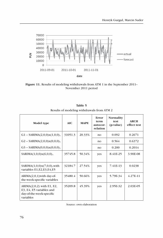
76
Henryk Gurgul, Marcin Suder
Figure 11. Results of modeling withdrawals from ATM 1 in the September 2011– November 2011 period
table 5
Results of modeling withdrawals from ATM 2
Model type Aic MApe
error term
autocor‑relation
Normality test
(p‑value)ArcH
effect test
G1 – SARIMA(2,0,0)x(1,0,0)7
G2 – SARIMA(2,0,0)x(0,0,0)7
G3 – SARIMA(0,0,0)x(0,0,0)7
31051.3 20.33% no 0.092 0.2671
no 0.564 0.6372
no 0.200 0.2014
SARIMA(1,0,0)x(6,0,0)7 35745.8 50.34% yes 8.41E-25 3.90E-08
SARIMA(1,0,0)x(7,0,0)7with variables E1,E2,E3,E4,E5
32184.7 27.54% yes 7.41E-13 0.0238
ARIMA(2,0,1)with day-of-the-week-specific variables
35480.4 50.66% yes 5.79E-34 4.27E-11
ARIMA(2,0,2) with E1, E2, E3, E4, E5 variables and day-of-the-week-specific variables
35209.8 45.39% yes 2.95E-32 2.03E-05
Source: own elaboration
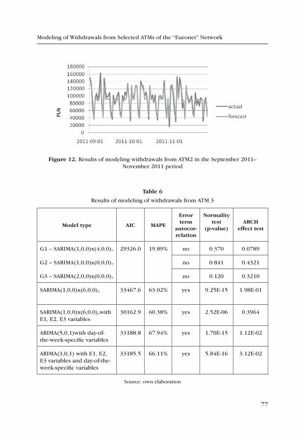
77
Modeling of Withdrawals from Selected ATMs of the “Euronet” Network
Figure 12. Results of modeling withdrawals from ATM2 in the September 2011– November 2011 period
table 6
Results of modeling of withdrawals from ATM 3
Model type Aic MApe
error term
autocor‑relation
Normality test
(p‑value)ArcH
effect test
G1 – SARIMA(1,0,0)x(4,0,0)7
G2 – SARIMA(1,0,0)x(0,0,0)7
G3 – SARIMA(2,0,0)x(0,0,0)7
29326.0 19.89% no 0.370 0.0789
no 0.841 0.4321
no 0.120 0.3210
SARIMA(1,0,0)x(6,0,0)7 33467.6 63.02% yes 9.25E-15 1.98E-01
SARIMA(1,0,0)x(6,0,0)7with E1, E2, E3 variables
30162.9 60.38% yes 2.52E-06 0.3964
ARIMA(5,0,1)with day-of-the-week-specific variables
33188.8 67.94% yes 1.70E-15 1.12E-02
ARIMA(3,0,1) with E1, E2, E3 variables and day-of-the-week-specific variables
33185.5 66.11% yes 5.84E-16 3.12E-02
Source: own elaboration
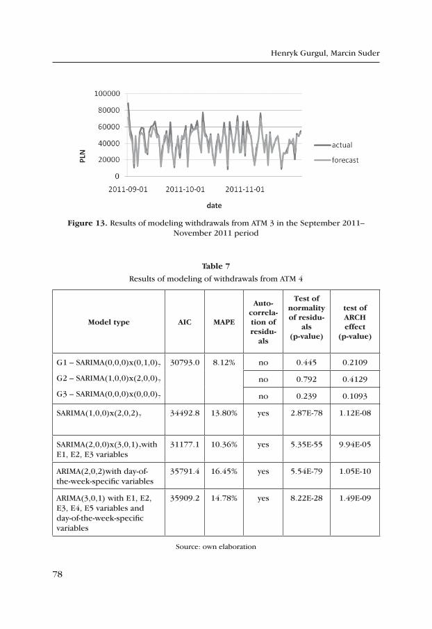
78
Henryk Gurgul, Marcin Suder
Figure 13. Results of modeling withdrawals from ATM 3 in the September 2011– November 2011 period
table 7
Results of modeling of withdrawals from ATM 4
Model type Aic MApe
Auto‑correla‑tion of residu‑
als
test of normality of residu‑
als (p‑value)
test of ArcH effect
(p‑value)
G1 – SARIMA(0,0,0)x(0,1,0)7
G2 – SARIMA(1,0,0)x(2,0,0)7
G3 – SARIMA(0,0,0)x(0,0,0)7
30793.0 8.12% no 0.445 0.2109
no 0.792 0.4129
no 0.239 0.1093
SARIMA(1,0,0)x(2,0,2)7 34492.8 13.80% yes 2.87E-78 1.12E-08
SARIMA(2,0,0)x(3,0,1)7with E1, E2, E3 variables
31177.1 10.36% yes 5.35E-55 9.94E-05
ARIMA(2,0,2)with day-of-the-week-specific variables
35791.4 16.45% yes 5.54E-79 1.05E-10
ARIMA(3,0,1) with E1, E2, E3, E4, E5 variables and day-of-the-week-specific variables
35909.2 14.78% yes 8.22E-28 1.49E-09
Source: own elaboration
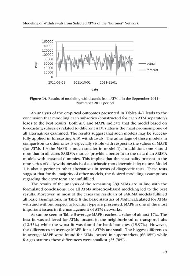
79
Modeling of Withdrawals from Selected ATMs of the “Euronet” Network
Figure 14. Results of modeling withdrawals from ATM 4 in the September 2011– November 2011 period
An analysis of the empirical outcomes presented in Tables 4–7 leads to the conclusion that modeling each subseries (constructed for each ATM separately) leads to the best results. Both AIC and MAPE indicate that the model based on forecasting subseries related to different ATM states is the most promising one of all alternatives examined. The results suggest that such models may be success-fully applied in forecasting ATM withdrawals. The advantage of these models in comparison to other ones is especially visible with respect to the values of MAPE (for ATMs 1-3 the MAPE is much smaller in model 1). In addition, one should note that in all cases SARIMA models provide a better fit to the data than ARIMA models with seasonal dummies. This implies that the seasonality present in the time series of daily withdrawals is of a stochastic (not deterministic) nature. Model 1 is also superior to other alternatives in terms of diagnostic tests. These tests suggest that for the majority of other models, the desired modeling assumptions regarding the error term are unfulfilled.
The results of the analysis of the remaining 289 ATMs are in line with the formulated conclusions. For all ATMs subseries-based modeling led to the best results. Moreover, in most of the cases the residuals of SARIMA models fulfilled all basic assumptions. In Table 8 the basic statistics of MAPE calculated for ATMs with and without respect to location type are presented. MAPE is one of the most important issues in the management of ATM networks.
As can be seen in Table 8 average MAPE reached a value of almost 17%. The best fit was achieved for ATMs located in the neighborhood of transport hubs (12.55%) while the worst fit was found for bank branches (19.97%). However, the differences in average MAPE for all ATMs are small. The biggest differences in average MAPE were found for ATMs located in supermarkets (66.68%) while for gas stations these differences were smallest (25.70%) .
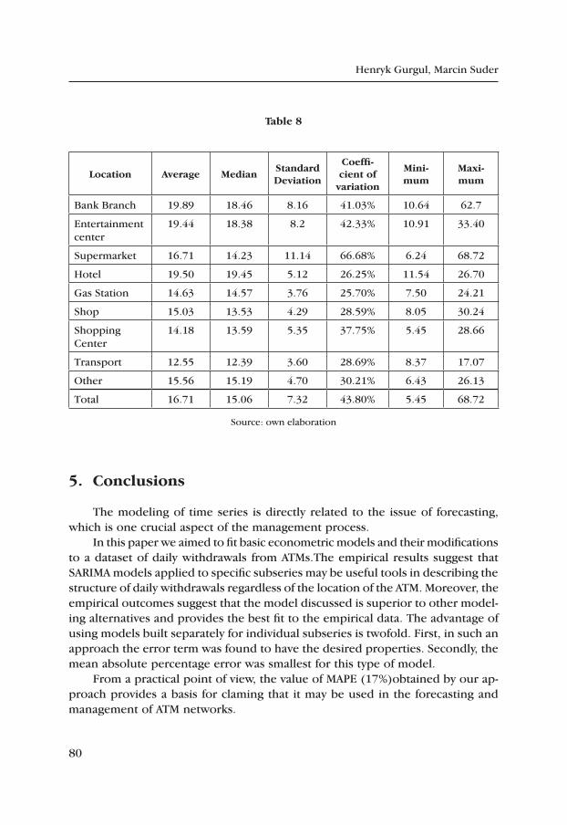
80
Henryk Gurgul, Marcin Suder
table 8
Location Average MedianStandard Deviation
coeffi‑cient of
variation
Mini‑mum
Maxi‑mum
Bank Branch 19.89 18.46 8.16 41.03% 10.64 62.7
Entertainment center
19.44 18.38 8.2 42.33% 10.91 33.40
Supermarket 16.71 14.23 11.14 66.68% 6.24 68.72
Hotel 19.50 19.45 5.12 26.25% 11.54 26.70
Gas Station 14.63 14.57 3.76 25.70% 7.50 24.21
Shop 15.03 13.53 4.29 28.59% 8.05 30.24
Shopping Center
14.18 13.59 5.35 37.75% 5.45 28.66
Transport 12.55 12.39 3.60 28.69% 8.37 17.07
Other 15.56 15.19 4.70 30.21% 6.43 26.13
Total 16.71 15.06 7.32 43.80% 5.45 68.72
Source: own elaboration
5. conclusions
The modeling of time series is directly related to the issue of forecasting, which is one crucial aspect of the management process.
In this paper we aimed to fit basic econometric models and their modifications to a dataset of daily withdrawals from ATMs.The empirical results suggest that SARIMA models applied to specific subseries may be useful tools in describing the structure of daily withdrawals regardless of the location of the ATM. Moreover, the empirical outcomes suggest that the model discussed is superior to other model-ing alternatives and provides the best fit to the empirical data. The advantage of using models built separately for individual subseries is twofold. First, in such an approach the error term was found to have the desired properties. Secondly, the mean absolute percentage error was smallest for this type of model.
From a practical point of view, the value of MAPE (17%)obtained by our ap-proach provides a basis for claming that it may be used in the forecasting and management of ATM networks.
81
Modeling of Withdrawals from Selected ATMs of the “Euronet” Network
references
[1] Amromin E., Chakravorti S., Debit card and cash usage: a cross-country analysis, Technical report, Federal Reserve Bank of Chicago, 2007.
[2] Bell W.R., Hillmer S.C., Modeling Time Series with Calendar Variation, “Journal of the American Statistical Association” 1983, 78, pp. 526–534.
[3] Boeschoten W.C., Cash management, payment patterns and the demand for money,“De Economist” 1998, 146, pp. 117–42.
[4] Brentnall A.R., Crowder M.J., Hand, D.J., A statistical model for the tempo-ral pattern of individual automated teller machine withdrawals, “Applied Statistics” 2008, 57, Part 1, pp. 43–59.
[5] Brentnall A.R., Crowder M.J., Hand D.J., Predicting the amount individuals withdraw at cash machines using a random effects multinomial model, “Statistical Modelling” 2010, 10(2), pp. 197–214.
[6] Carlsen M., Storgaard P.E., Dankort payments as a timely indicator of retail sales in Denmark, Danmarks Nationalbank Working Papers, No. 66, 2010.
[7] Cleveland W. S., Devlin S.J., Calendar Effects in Monthly Time Series: Detec-tion by Spectrum Analysis and Graphical Methods, “Journal of the American Statistical Association” 1980, 371, 75, pp. 487–496.
[8] Cleveland W.P., Grupe M.R., Modeling time series when calendar effects are present, Applied Time Series Analysis of Economic Data, ed. A. Zellner, U.S. Department of Commerce, U.S. Bureau of the Census, Washington D.C., 1983, pp. 57–67.
[9] Esteves P.S., Are ATM/POS Data Relevant When Now casting Private Con-sumption?, Banco de Portugal Working Paper, 25, 2009.
[10] Findley D.F., Monsell B.C., Modeling Stock Trading Day Ef fects Under Flow Day-of-Week Effect Constraints, “Journal of Official Statistics” 2009, Vol. 25(3), pp. 415–430.
[11] Findley D.F., Monsell B.C., Bell W.R., Otto M.C., Chen B.C., New capabilities and Methods of the X-12-ARIMA seasonal adjustment program, “Journal of Business and Economic Statistics” 1998, vol. 16(2), pp. 127–177.
[12] Findley D.F., Soukup R.J., On the Spectrum Diagnostics Used by X-12-ARIMA to Indicate the Presence of Trading Day Effects after Modeling or Adjustment, “Proceedings of the American Statistical Association, Business and Statistics Section” 1999, pp. 144–149.
[13] Findley D.F., Soukup R.J., Modeling and Model Selection for Moving Holi-days, “Proceedings of the American Statistical Association, Business and Economics Statistics Section” 2000, pp. 102–107.
[14] Findley D.F., Soukup R.J., Detection and Modeling of Trading Day Effects, in: ICES II: Proceedings of the Second Inter national Conference on Economic Surveys, 2001, pp. 743–753.

Henryk Gurgul, Marcin Suder
[15] Galbraith J.W., Tkacz G., Electronic Transactions as High-Frequency Indica-tors of Economic Activity, Bank of Canada Working Paper, 2007-58.
[16] Gerdes G.R., Walton J.K., Liu M.X, Parke D.W., Trends in the Use of Payment Instruments in the United States, Federal Reserve Bulletin 91 (Spring), 2005, pp. 180–201.
[17] Gurgul G., Suder M., Efekt kalendarza wypłat z bankomatów sieci Euronet, Zeszyt Naukowy nr 8, WSEI, Kraków 2012, s. 25–42.
[18] Gurgul H., Suder M., Empiryczne własności wielkości dziennych wypłat z bankomatów na przykładzie sieci bankomatów firmy EURONET z terenu województw: małopolskiego i podkarpackiego, to appear.
[19] Hansen P.R., Lunde A., Nason J.M., Testing the Significance of Calendar Ef-fects, Working Paper 2005-2, Federal Reserve Bank of Atlanta, 2005.
[20] Hand D.J., Blunt G., Prospecting for gems in credit card data,IMA “Journal of Management Mathematics” 2001, 12, pp.173–200.
[21] Kufel T., Ekonometryczna analiza cykliczności procesów gospodarczych o wysokiej częstotliwości obserwowania, Wydawnictwo Naukowe Uniwer-sytety Mikołaja Kopernika, Toruń 2010.
[22] Liu L.M., Analysis of Time Series with Calendar Effects, “Manage ment Science” 1980, 26, pp. 106–112.
[23] McElroy T.S., Holland S., A Nonparametric Test for Assessing Spectral Peaks, Research Report 2005-10, Statistical Research Division, U.S. Bureau of the Census, Washington D.C., 2005.
[24] Rodrigues P., Esteves P., Calendar effects in daily ATM withdrawals, “Eco-nomics Bulletin” 2010, Vol. 30, no. 4, pp. 2587–2597.
[25] Schmitz S., Wood G., Institutional Change in the Payments System and Monetary Policy, Routledge London, 2006.
[26] Simutis R., Dilijonas D., Bastina L., Cash demand forecasting for ATM using Neural Networks and support vector regression algorithms, 20th Interna-tional Conference, EURO Mini Conference, “Continuous Optimization and Knowledge-Based Technologies” (EurOPT-2008), Selected Papers, Vilnius May 20–23, 2008, pp. 416–421.
[27] Snellman H., Viren M., ATM networks and cash usage, “Applied Financial Economics” 2009, 19 (10), pp. 841–851.
[28] Takala K., Viren M., Impact of ATMs on the Use of Cash, “Communications and Strategies” 2007, No 66, pp. 47–61.
[29] Young A.H., Estimating Trading-day Variation in Monthly Economic Time Series, Technical Paper 12, Bureau of the Census, 1965.
83
Managerial Economics2013, No. 13, pp. 83–98
http://dx.doi.org/10.7494/manage.2013.13.83
Katarzyna Liczmańska*, Agnieszka M. Wiśniewska**
A Strong Brand as a Determinant of purchase the case of Sectors, where Advertising in Mass Media is Banned – on the example of the polish Spirits Sector
1. introduction
In order to achieve success a company must continually search for develop-ment opportunities, respond to change with new or improved products, tech-nologies, and marketing activities to achieve a competitive advantage over other participants on the market [3, 170].
Marketing departments compete to find innovative products as well as in-teresting means and channels of communication to gain and retain clients. The clients’ contentment and satisfaction lead to repeat purchase and even recom-mendations, which in turn is an affirmation of the company’s right of existence. Regular purchase loyalty contributes to an increase in market share, while positive attitudes accompanying loyalty allow companies to raise prices [2, 82]. Eventually all the above result in the company’s profit.
A powerful tool combining rationally evaluated functional values based on results and facts with emotional values which are subject to affective evaluation is a strong brand [5, 20]. A brand gives identity to a product defined in the last cen-tury by Ph. Kotler as anything offered to potential buyers to satisfy their needs or desires. A brand also distinguishes the product from its competitors. A brand helps avoid using prices as an instrument of competition, this usually means a decrease in company sales if its competitors offer a similar price. A company with strong brands ensures itself a better competing position, higher profit margins [7, 25–26], loyal customers [10, 45], as well as a larger support from sales intermediaries [10, 49].
* Nicolaus Copernicus University, Faculty of Economic Sciences and Management, The Department of Enterprise Management.
** University of Promotion, Warsaw

84
Katarzyna Liczmańska, Agnieszka M. Wiśniewska
A brand is a constant element identifying the producer with the product [8, 65]. As it is a complex entity, it comprises a combination of functional and emo-tional values desired and sought for by the customer [14, 340]. It is a composition of numerous elements containing intensified messages which aim to distinguish one commodity or product from all other competing products [16, 87].
The authors’ thesis is that a strong brand is the key determinant of market success in the Polish spirits sector. What’s interesting is the fact that advertising plays a major role in the building and promotion of brands, while advertising in mass media is completely banned in the spirits sector. The main law banning advertising in this sector is the Act on Alcohol Abuse and Alcoholism Prevention of 26 October 1982 1. Considering the above, communication with customers poses a challenge and alcohol producers have a difficult task of attracting customers to their products, especially to the new ones.
The main beverage in the spirits category is plain vodka, where the contents of each bottle can be brought down to grain alcohol and water. Despite the differ-ences in recipes and production technologies, customers may be of the opinion that these products are in fact one and the same and only differ slightly in taste. In this situation the producer has to reach the potential customers informing them about the quality of the offer and persuade the customers to consider that particular product as unique and make them buy it [15, 182–185].
Advertising restrictions impede communication with the customer on a large scale. Budgets are shifted from ATL class media (Above-The-Line; media such as television, radio, press, cinema, outdoor, internet) to selected promotional BTL forms (Below-The-Line; forms such as sales promotion, merchandising etc). Pre-senting a new product and building brand awareness requires the use of mass media tools and that is why limited use of advertising reduces the number of new brands being launched on the market. Difficulties in creating new strong brands forces alcohol producers to focus on the strength and value of the brands, or on the already existing brands which, from the customer’s point of view act as a guarantee of quality of the product and of the production process. Thus the second thesis which logically complements the presented theses model is that, despite the legal restrictions in advertising and promotion it is possible to act in support of the strength of spirits brands. A strong brand shall be understood as a brand with a relatively high brand awareness [11, 380], appreciated by buyers [3, 7], having a strong position on the market [8, 67].
2. A background of marketing activities in the spirits sector
In Poland in the 80’s there was no clear distinction between vodka brands. Each Polmos2 could produce all the brands existing on the market. Therefore the
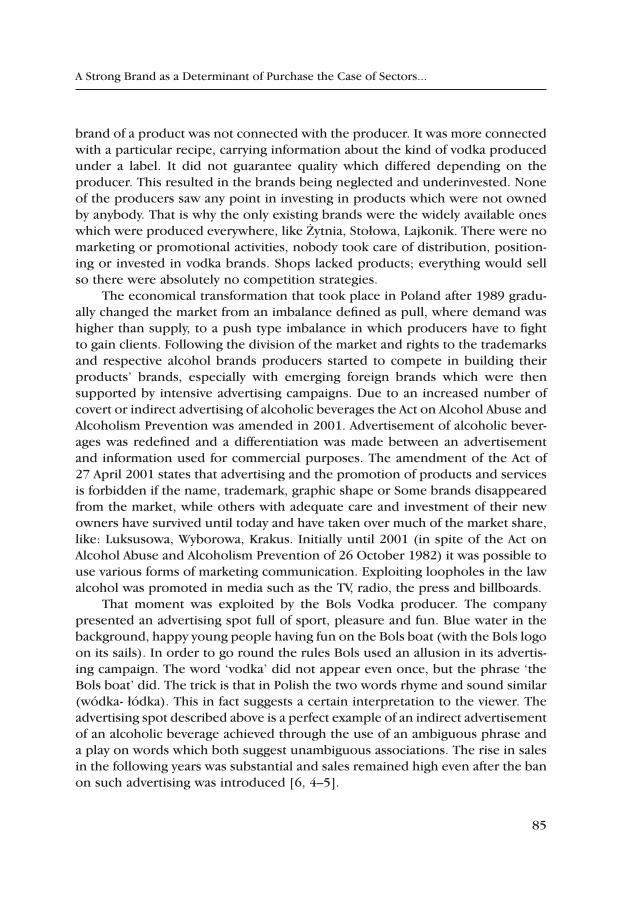
85
A Strong Brand as a Determinant of Purchase the Case of Sectors...
brand of a product was not connected with the producer. It was more connected with a particular recipe, carrying information about the kind of vodka produced under a label. It did not guarantee quality which differed depending on the producer. This resulted in the brands being neglected and underinvested. None of the producers saw any point in investing in products which were not owned by anybody. That is why the only existing brands were the widely available ones which were produced everywhere, like Żytnia, Stołowa, Lajkonik. There were no marketing or promotional activities, nobody took care of distribution, position-ing or invested in vodka brands. Shops lacked products; everything would sell so there were absolutely no competition strategies.
The economical transformation that took place in Poland after 1989 gradu-ally changed the market from an imbalance defined as pull, where demand was higher than supply, to a push type imbalance in which producers have to fight to gain clients. Following the division of the market and rights to the trademarks and respective alcohol brands producers started to compete in building their products’ brands, especially with emerging foreign brands which were then supported by intensive advertising campaigns. Due to an increased number of covert or indirect advertising of alcoholic beverages the Act on Alcohol Abuse and Alcoholism Prevention was amended in 2001. Advertisement of alcoholic bever-ages was redefined and a differentiation was made between an advertisement and information used for commercial purposes. The amendment of the Act of 27 April 2001 states that advertising and the promotion of products and services is forbidden if the name, trademark, graphic shape or Some brands disappeared from the market, while others with adequate care and investment of their new owners have survived until today and have taken over much of the market share, like: Luksusowa, Wyborowa, Krakus. Initially until 2001 (in spite of the Act on Alcohol Abuse and Alcoholism Prevention of 26 October 1982) it was possible to use various forms of marketing communication. Exploiting loopholes in the law alcohol was promoted in media such as the TV, radio, the press and billboards.
That moment was exploited by the Bols Vodka producer. The company presented an advertising spot full of sport, pleasure and fun. Blue water in the background, happy young people having fun on the Bols boat (with the Bols logo on its sails). In order to go round the rules Bols used an allusion in its advertis-ing campaign. The word ‘vodka’ did not appear even once, but the phrase ‘the Bols boat’ did. The trick is that in Polish the two words rhyme and sound similar (wódka- łódka). This in fact suggests a certain interpretation to the viewer. The advertising spot described above is a perfect example of an indirect advertisement of an alcoholic beverage achieved through the use of an ambiguous phrase and a play on words which both suggest unambiguous associations. The rise in sales in the following years was substantial and sales remained high even after the ban on such advertising was introduced [6, 4–5].
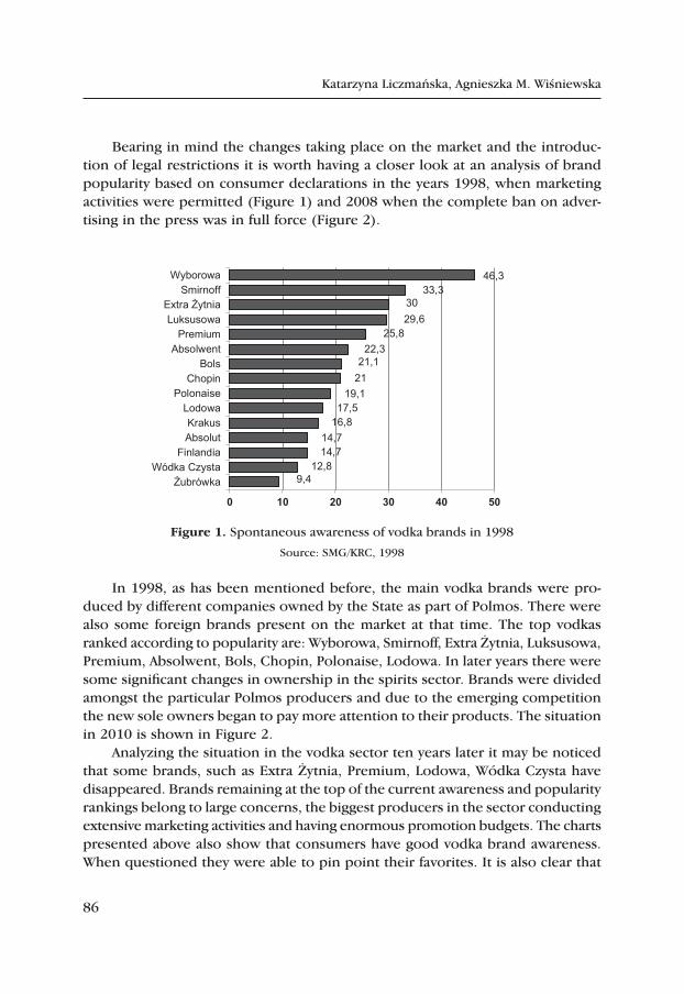
86
Katarzyna Liczmańska, Agnieszka M. Wiśniewska
Bearing in mind the changes taking place on the market and the introduc-tion of legal restrictions it is worth having a closer look at an analysis of brand popularity based on consumer declarations in the years 1998, when marketing activities were permitted (Figure 1) and 2008 when the complete ban on adver-tising in the press was in full force (Figure 2).
Figure 1. Spontaneous awareness of vodka brands in 1998
Source: SMG/KRC, 1998
In 1998, as has been mentioned before, the main vodka brands were pro-duced by different companies owned by the State as part of Polmos. There were also some foreign brands present on the market at that time. The top vodkas ranked according to popularity are: Wyborowa, Smirnoff, Extra Żytnia, Luksusowa, Premium, Absolwent, Bols, Chopin, Polonaise, Lodowa. In later years there were some significant changes in ownership in the spirits sector. Brands were divided amongst the particular Polmos producers and due to the emerging competition the new sole owners began to pay more attention to their products. The situation in 2010 is shown in Figure 2.
Analyzing the situation in the vodka sector ten years later it may be noticed that some brands, such as Extra Żytnia, Premium, Lodowa, Wódka Czysta have disappeared. Brands remaining at the top of the current awareness and popularity rankings belong to large concerns, the biggest producers in the sector conducting extensive marketing activities and having enormous promotion budgets. The charts presented above also show that consumers have good vodka brand awareness. When questioned they were able to pin point their favorites. It is also clear that
9,4 12,8
14,7 14,7
16,8 17,5
19,1 21 21,1
22,3 25,8
29,6 30
33,3 46,3
0 10 20 30 40 50
ŻubrówkaWódka Czysta
FinlandiaAbsolutKrakus
LodowaPolonaise
ChopinBols
AbsolwentPremium
LuksusowaExtra Żytnia
SmirnoffWyborowa
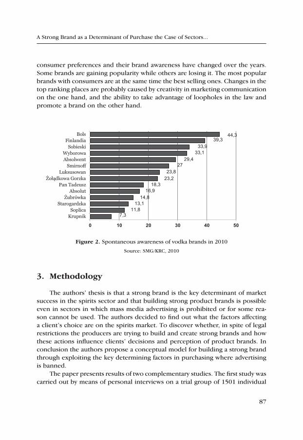
87
A Strong Brand as a Determinant of Purchase the Case of Sectors...
consumer preferences and their brand awareness have changed over the years. Some brands are gaining popularity while others are losing it. The most popular brands with consumers are at the same time the best selling ones. Changes in the top ranking places are probably caused by creativity in marketing communication on the one hand, and the ability to take advantage of loopholes in the law and promote a brand on the other hand.
Figure 2. Spontaneous awareness of vodka brands in 2010
Source: SMG/KRC, 2010
3. Methodology
The authors’ thesis is that a strong brand is the key determinant of market success in the spirits sector and that building strong product brands is possible even in sectors in which mass media advertising is prohibited or for some rea-son cannot be used. The authors decided to find out what the factors affecting a client’s choice are on the spirits market. To discover whether, in spite of legal restrictions the producers are trying to build and create strong brands and how these actions influence clients’ decisions and perception of product brands. In conclusion the authors propose a conceptual model for building a strong brand through exploiting the key determining factors in purchasing where advertising is banned.
The paper presents results of two complementary studies. The first study was carried out by means of personal interviews on a trial group of 1501 individual
7,3 11,8
13,1 14,8
16,9 18,3
23,2 23,8
27 29,4
33,1 33,9
39,3 44,3
0 10 20 30 40 50
KrupnikSoplica
StarogardzkaŻubrówka
AbsolutPan Tadeusz
Żołądkowa GorzkaLuksusowan
SmirnoffAbsolwentWyborowa
SobieskiFinlandia
Bols
88
Katarzyna Liczmańska, Agnieszka M. Wiśniewska
respondents in 2007 in Poland. The second study was carried out using personal or Internet questionnaires on a trial group of 16 companies producing or import-ing spirits. The companies offer the best known and the most significant alcohol brands having 95.95% of the market share.
The analyses of the results made it possible to determine that a strong brand is not only the key asset in the spirits sector (in a situation where advertising is banned), but is also the determining factor in the clients’ purchasing decision.
4. Key decision elements in vodka purchase
The process of purchasing vodka is similar to the purchase of other consumer goods the only problem being an impeded communication between the brand owner and the consumer. Figure 3 shows elements which decide in the process of selecting a brand by the consumer.
Figure 3. Key decision elements in the process of spirits purchase
Source: K. Liczmańska, own research, personal interview, 2007, N= 1501 individual respondents
Respondents first mention a strong brand and the exposition of a product, which in fact aids awareness and recollection of a brand [23, 214] – 87.5% for each option. In the analyzed sector it is, therefore the ability to build a strong brand and maintain it that plays a key role. Looking At responses supplied by consumers it is impossible not to notice how great the influence of vodka producers and their marketing activities is on the preferences and purchase decisions of consumers.
6,25
12,5
12,5
31,25
31,25
37,5
43,75
43,75
56
56
68,75
81,25
87,5
87,5
0 10 20 30 40 50 60 70 80 90 100
Polish productForeign product
Trust in the producerHabit
Friend's opinionPackaging
AvailabilityTaste of the product
PricePromotion with a gift
Fashionability of the brandHigh quality
ExpositionStrong brand
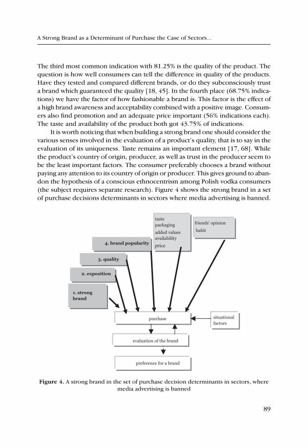
89
A Strong Brand as a Determinant of Purchase the Case of Sectors...
The third most common indication with 81.25% is the quality of the product. The question is how well consumers can tell the difference in quality of the products. Have they tested and compared different brands, or do they subconsciously trust a brand which guaranteed the quality [18, 45]. In the fourth place (68.75% indica-tions) we have the factor of how fashionable a brand is. This factor is the effect of a high brand awareness and acceptability combined with a positive image. Consum-ers also find promotion and an adequate price important (56% indications each). The taste and availability of the product both got 43.75% of indications.
It is worth noticing that when building a strong brand one should consider the various senses involved in the evaluation of a product’s quality, that is to say in the evaluation of its uniqueness. Taste remains an important element [17, 68]. While the product’s country of origin, producer, as well as trust in the producer seem to be the least important factors. The consumer preferably chooses a brand without paying any attention to its country of origin or producer. This gives ground to aban-don the hypothesis of a conscious ethnocentrism among Polish vodka consumers (the subject requires separate research). Figure 4 shows the strong brand in a set of purchase decisions determinants in sectors where media advertising is banned.
Figure 4. A strong brand in the set of purchase decision determinants in sectors, where media advertising is banned
purchase
friends’ opinion
habit
situational factors
1. strong brand
3. quality
taste packaging
added values availability
price
evaluation of the brand
preference for a brand
2. exposition
4. brand popularity
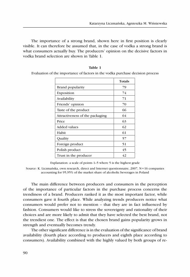
90
Katarzyna Liczmańska, Agnieszka M. Wiśniewska
The importance of a strong brand, shown here in first position is clearly visible. It can therefore be assumed that, in the case of vodka a strong brand is what consumers actually buy. The producers’ opinion on the decisive factors in vodka brand selection are shown in Table 1.
table 1
Evaluation of the importance of factors in the vodka purchase decision process
totals
Brand popularity 79
Exposition 74
Availability 71
Friends’ opinion 70
Taste of the product 66
Attractiveness of the packaging 64
Price 63
Added values 62
Habit 61
Quality 57
Foreign product 51
Polish product 45
Trust in the producer 42
Explanation: a scale of points 1–5 where 5 is the highest grade
Source: K. Liczmańska, own research, direct and Internet questionnaire, 2007, N=16 companies accounting for 95,95% of the market share of alcoholic beverages in Poland
The main difference between producers and consumers in the perception of the importance of particular factors in the purchase process concerns the trendiness of a brand. Producers ranked it as the most important factor, while consumers gave it fourth place. While analyzing trends producers notice what consumers would prefer not to mention – that they are in fact influenced by fashion. Consumers would like to stress the sovereignty and rationality of their choices and are more likely to admit that they have selected the best brand, not the trendiest one. The effect is that the chosen brand gains popularity grows in strength and eventually becomes trendy.
The other significant difference is in the evaluation of the significance of brand availability (fourth place according to producers and eighth place according to consumers). Availability combined with the highly valued by both groups of re-
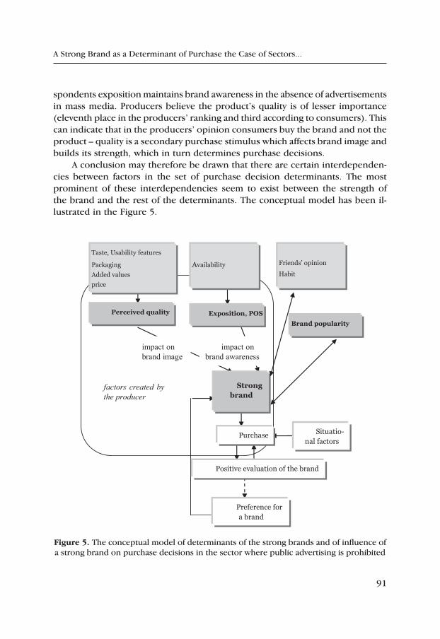
91
A Strong Brand as a Determinant of Purchase the Case of Sectors...
spondents exposition maintains brand awareness in the absence of advertisements in mass media. Producers believe the product’s quality is of lesser importance (eleventh place in the producers’ ranking and third according to consumers). This can indicate that in the producers’ opinion consumers buy the brand and not the product – quality is a secondary purchase stimulus which affects brand image and builds its strength, which in turn determines purchase decisions.
A conclusion may therefore be drawn that there are certain interdependen-cies between factors in the set of purchase decision determinants. The most prominent of these interdependencies seem to exist between the strength of the brand and the rest of the determinants. The conceptual model has been il-lustrated in the Figure 5.
Figure 5. The conceptual model of determinants of the strong brands and of influence of a strong brand on purchase decisions in the sector where public advertising is prohibited
Strong brand
Exposition, POS Perceived quality
Brand popularity
Taste, Usability features
Packaging Added values price
Availability
Friends’ opinion
Habit
Situatio-nal factors
Purchase
Positive evaluation of the brand
impact on brand awareness
impact on brand image
factors created by the producer
Preference for a brand

92
Katarzyna Liczmańska, Agnieszka M. Wiśniewska
Brand awareness and brand image are the key construction elements of brand strength. A strong brand specializes in supplying the consumer with exceptional benefits. A strong brand is well-known by consumers and plays an important role in meeting their needs, is respected and has prestige.
In sectors where there is a ban on alcohol advertising in mass media produc-ers exploit other stimuli within the set of purchase decision determinants to build strong brands. Companies retained control over stimuli which are important for buyers such as product display in points of sale and availability, which is a sine qua non condition for display management. Quality is also important although it is a rather subjective form of evaluation based on factors such as taste or other product traits, packaging, price and added value.
Investing in tools which affect consumers’ evaluation of product quality and at the same time ensure adequate product exposure at point of sale means that a company is able to build a strong brand without advertising in mass media.
Fashion, understood as a commonly accepted or even desired style in a given social group is a temporary phenomenon. It is, on the one hand the effect of brand strength, and on the other it increases brand strength. A company may either build on that effect, and create a stable market position for the brand, or it may loose the opportunity and let the interest in the brand pass with the fashion – it largely depends on marketing management skills. When a brand is in fashion the company should build consumers’ appreciation. Then, regardless of the trends the brand’s strength will be supported by purchase habits (brand market share) and by recommendations to friends (brand awareness and brand image).
5. the benefits producers get from strong brands
In order to beat its competition a company should decide which of its as-sets, processes and functions is most suitable to achieve this. Attributes such as a low price, innovative technology or even a good distribution chain are all easily duplicated by competitors so the more desired attributes are those which cannot be easily copied and provide the company with a lasting competitive advantage.
The assets theory states that assets and abilities that are rare, lasting, imper-fectly mobile and difficult to imitate enable the company to gain a sustainable competitive advantage [2, 97]. Companies usually build their strategies basing simultaneously on various attributes, one of them is almost always a brand because branded products are chosen more frequently than unbranded ones [20, 220].
Vodka consumers and producers confirm that strong brands do exist in the vodka sector, although advertising in mass media is completely banned. All
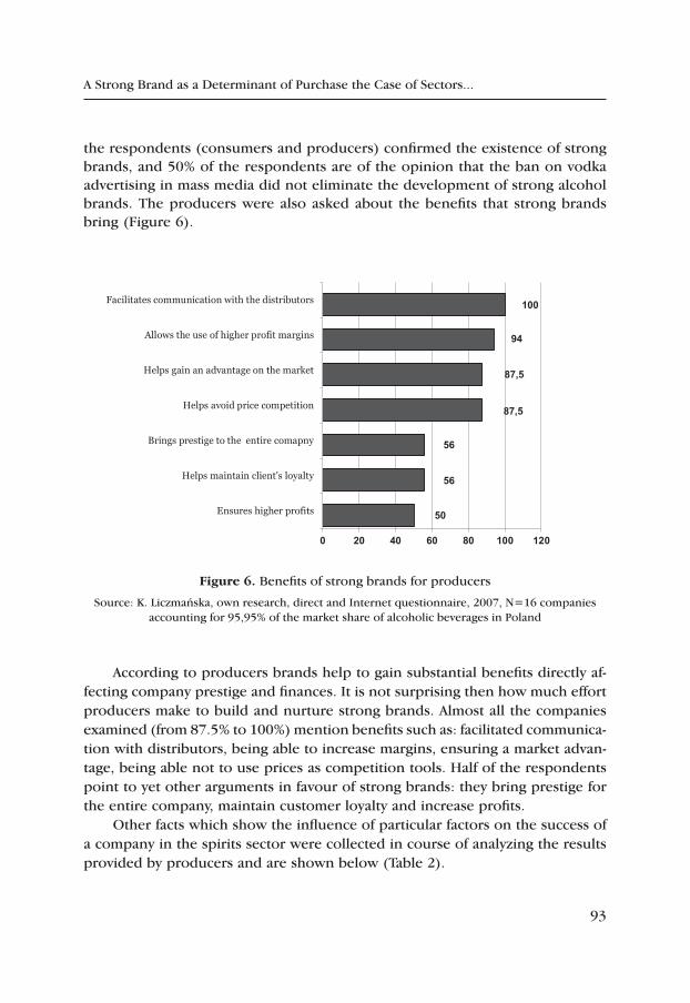
93
A Strong Brand as a Determinant of Purchase the Case of Sectors...
the respondents (consumers and producers) confirmed the existence of strong brands, and 50% of the respondents are of the opinion that the ban on vodka advertising in mass media did not eliminate the development of strong alcohol brands. The producers were also asked about the benefits that strong brands bring (Figure 6).
Figure 6. Benefits of strong brands for producers
Source: K. Liczmańska, own research, direct and Internet questionnaire, 2007, N=16 companies accounting for 95,95% of the market share of alcoholic beverages in Poland
According to producers brands help to gain substantial benefits directly af-fecting company prestige and finances. It is not surprising then how much effort producers make to build and nurture strong brands. Almost all the companies examined (from 87.5% to 100%) mention benefits such as: facilitated communica-tion with distributors, being able to increase margins, ensuring a market advan-tage, being able not to use prices as competition tools. Half of the respondents point to yet other arguments in favour of strong brands: they bring prestige for the entire company, maintain customer loyalty and increase profits.
Other facts which show the influence of particular factors on the success of a company in the spirits sector were collected in course of analyzing the results provided by producers and are shown below (Table 2).
50
56
56
87,5
87,5
94
100
0 20 40 60 80 100 120
Ensures higher profits
Helps maintain client's loyalty
Brings prestige to the entire comapny
Helps avoid price competition
Helps gain an advantage on the market
Allows the use of higher profit margins
Facilitates communication with the distributors
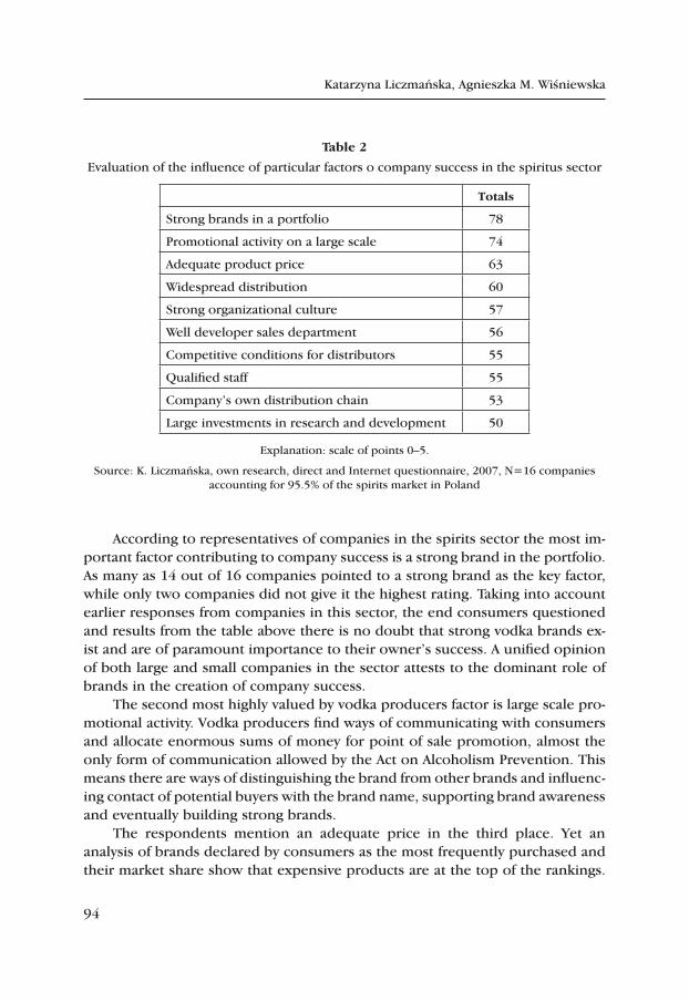
94
Katarzyna Liczmańska, Agnieszka M. Wiśniewska
table 2
Evaluation of the influence of particular factors o company success in the spiritus sector
totals
Strong brands in a portfolio 78
Promotional activity on a large scale 74
Adequate product price 63
Widespread distribution 60
Strong organizational culture 57
Well developer sales department 56
Competitive conditions for distributors 55
Qualified staff 55
Company’s own distribution chain 53
Large investments in research and development 50
Explanation: scale of points 0–5.
Source: K. Liczmańska, own research, direct and Internet questionnaire, 2007, N=16 companies accounting for 95.5% of the spirits market in Poland
According to representatives of companies in the spirits sector the most im-portant factor contributing to company success is a strong brand in the portfolio. As many as 14 out of 16 companies pointed to a strong brand as the key factor, while only two companies did not give it the highest rating. Taking into account earlier responses from companies in this sector, the end consumers questioned and results from the table above there is no doubt that strong vodka brands ex-ist and are of paramount importance to their owner’s success. A unified opinion of both large and small companies in the sector attests to the dominant role of brands in the creation of company success.
The second most highly valued by vodka producers factor is large scale pro-motional activity. Vodka producers find ways of communicating with consumers and allocate enormous sums of money for point of sale promotion, almost the only form of communication allowed by the Act on Alcoholism Prevention. This means there are ways of distinguishing the brand from other brands and influenc-ing contact of potential buyers with the brand name, supporting brand awareness and eventually building strong brands.
The respondents mention an adequate price in the third place. Yet an analysis of brands declared by consumers as the most frequently purchased and their market share show that expensive products are at the top of the rankings.
95
A Strong Brand as a Determinant of Purchase the Case of Sectors...
An adequate price however may not mean a low price, as it is the consumer’s acceptance of a price for the quality of the product and the value added by the brand that is important for the company’s success.
A wide distribution is the fourth important factor indicated by company rep-resentatives. As has been noted in the consumer study product availability plays a relatively important role in the purchase of vodka. A consumer who does not find his favourite vodka brand on the shelf simply buys a different brand, often tempted by an attractive promotion. In this particular sector, where communication with the consumer may be established virtually only at point of sale product avail-ability and ensuring its presence in distribution channels is of primary importance.
Other factors such as a strong organizational culture, a well-developed sales department, competitive conditions for distributors, qualified staff, a distribu-tion chain owned by the company and investment in research and development were rated as less important, which does not mean they do not play any role in building company success. The well- developed sales department is of particular interest. It has been noticed that excellent product display and activities at point of sale are key elements in the consumer’s selection process of vodka brands. Consequently, a well-developed sales department owned by the company where sales representatives have direct access to points of sale seems to affect company success in this sector. However, market observation has shown that companies with smaller sales departments employ the wholesalers’ representatives. They work as merchandisers as well as brand ambassadors playing an important role in the communication process between producers and retailers.
A brand considered in the context of its name, value or loyalty became decades ago a powerful force in business which can be shaped and managed [19, 78]. The significance of the brand as a tool of communication between the company and the buyers increases proportionally to the need for differentiating the product from competitors’ products and the need for its identification [13, 98].
A strong brand enjoying a group of loyal consumers almost ‘sells itself’. Re-search has shown that consumers know which brand they want to buy and do precisely that once in the shop. Their favourite brands are often the leaders in both popularity rankings and market share. Promotions noticed by consumers belonged to brands which were most frequently purchased when the decision was made just before purchase at the store. Consumers notice strong brands and have their own preferences. When asked if they were aware of marketing activity on the part of vodka producers, 89% said yes.
Two models of consumer behaviour may be noticed in which the brand and promotion make consumers aware of its existence and its benefits, at the same time playing a major role in the decision. In the first model the consumer goes to a retailer with the intention of buying a particular (preferred) brand of
96
Katarzyna Liczmańska, Agnieszka M. Wiśniewska
alcohol. It is important for the brand to be available. Otherwise promotional activities of other brands at the point of sale will shift the consumer’s attention to another known brand or even initiate interest in a completely new one. The second model assumes that the consumer goes to the retailer with the intention of buying vodka, but without preference for a particular brand or considering one of many brands [22, 30]. Hence the final decision depends on availability and communication activity provided for the brand by the producer. In both cases the brand often bought and consumed in circumstances marking a special event such as a birthday party or other celebration may become a brand the consumer will return to in the future. It could be described as pull effect. Strong brands facilitate producers’ activities in distribution channels.
A consumer is ready to pay more for his favourite brand than for other brands which ensures a higher profit for the producer. It also allows distribution channels to set higher margins. Such a situation is very beneficial for the brand producer because both the wholesalers and retailers are willing to sell products at a higher margin to earn more.
An established brand transfers its strength and prestige to the entire company. This fact is exploited by companies in the spirits sector. The Bols Company has taken its name from its main brand Bols Vodka. The Sobieski Vodka is another example, its owner being Sobieski Company. Other examples include vodkas like Wybrowa, Luksusowa. It is easier to launch products under a known brand name and this occurs in the case of the most popular vodka brands. The brands are expanded to include new flavours, products in various price ranges or even different beverages altogether, such as RTD drinks, liqueurs, and other kinds of alcoholic beverages.
6. conclusions
In the highly competitive market of strong alcoholic beverages with the ban on advertising in mass media which would greatly help in influencing purchase decisions, a distinguishable brand becomes one of the key elements of a competi-tive advantage and a guarantee of success.
Analyses of the research conducted have shown that a strong brand is vodka’s greatest asset. Consumers notice them and buy products of established brands. Producers manage to carry out promotional activities well in spite of the ban on advertising in mass media. They are effective enough to be noticed by consumers who consciously choose vodka brands. Vodka brands which have been success-fully positioned in the highest places in consumers’ awareness are at the same time the best selling brands.
97
A Strong Brand as a Determinant of Purchase the Case of Sectors...
The material collected supported the thesis that consumers point to a strong brand as the key factor in choosing high end vodkas. All producer representa-tives stress the need to build strong brands and declare having such brands in their offer. This confirms the thesis put forward by the authors of this paper. The research clearly shows that alcohol producers believe building and sustaining strong brands to be the main source of competitive advantage. Producers know the market well as consumers point to all factors associated with the brand as key elements influencing their choices of vodka brands. A strong, well-known brand is very important. Undoubtedly a strong brand is the most important competitive asset a company may have in the vodka sector.
More and more companies believe that brands may be treated as company assets whose value may be reflected in the balance sheet, at the same time in-creasing company value. The growing importance of the brand is emphasized by L.B. Upshaw: ‘brands have become the core of contemporary, consumer oriented capitalistic economy where the mutual effect of brands enlivens trade exchange’ (Upshaw, 1995, p. 11). The vodka sector described above is not an exception and, in spite of the tight restrictions concerning alcohol advertisements in mass media, strong vodka brands exist and producers take good care of them. This is not in the least surprising as strong brands are key success factors.
references
[1] Aaker D.A., Building Strong Brands, “The Free Press”, New York 1999.[2] Amit R., Schoemaker P., Strategic assets and organizational rent, “Strategic
Management Journal”, Vol. 14/1993, pp. 33–46.[3] Arslan F.M., Altuna O.K., The effect of brand extensions on product brand
image, “Journal of Product & Brand Management” 2010, Vol 19, Issue 3, pp. 170–180.
[4] Chaudhuri A., Holbrook M.B., The chain of effects from brand trust and brand affect to brand performance: the role of brand loyalty, “Journal of Marketing”, Vol. 65, No. 2, pp. 81–93.
[5] de Chernatony L., Marka. Wizja i tworzenie marki, Gdańskie Wydawnictwo Psychologiczne, Gdańsk 2003.
[6] Dąbrowska K., Marketing alkoholu w Polsce, „Remedium” 2006, Vol. 10, pp. 4–5.
[7] Farquhar P.H., Managing brand equity, “Marketing Research” 1989, Vol. 1, September, pp. 24–33.
[8] Grzegorczyk A., Reklama, Polskie Wydawnictwo Ekonomiczne, Warszawa 2010.
[9] Kall J., Silna marka, Polskie Wydawnictwo Ekonomiczne, Warszawa 2001.
Katarzyna Liczmańska, Agnieszka M. Wiśniewska
[10] Keller K.L., Strategic Brand Management: Building, Measuring and Manag-ing Brand Equity, Prentice-Hall, Upper Saddle River, New York 2008.
[11] Kimpakorn N., Tocquer G., Service Brand equity and employee brand commitment, “Journal of Services Marketing” 2010, Volume 24, Issue 5, pp. 378–388.
[12] Kotler Ph., Marketing. Analiza, planowanie, wdrażanie i kontrola, Wydaw-nictwo Rebis, Warszawa 2005.
[13] Kotler Ph., Keller K.L., Marketing Management 12e, Pearson Prentice Hall, Upper Saddle River 2006.
[14] Kozłowska A., Reklama. Techniki perswazyjne, Oficyna Wydawnicza Szkoła Główna Handlowa w Warszawie, Warszawa 2011.
[15] Liczmańska K., Efekt kraju pochodzenia produktu a decyzje nabywcze kon-sumentów sektora alkoholi wysokoprocentowych, Roczniki Ekonomiczne Kujawsko-Pomorskiej Szkoły Wyższej w Bydgoszczy 2010, No. 3, pp. 177–187.
[16] Liczmańska K., Silna marka jako źródło przewagi konkurencyjnej w mo-mencie zakupu, Roczniki Ekonomiczne Kujawsko-Pomorskiej Szkoły Wyższej w Bydgoszczy 2008, No. 1, pp. 87–99.
[17] Lindstrom M., Brand Sense: Build Powerful Brands Through Touch, Taste, Smell, Sight and Sound, Free Press, New York 2005.
[18] Maison D., Utajone postawy konsumenckie, Gdańskie Wydawnictwo Psy-chologiczne, Gdańsk 2004.
[19] Marconi J., Marketing marki. W jaki sposób tworzyć, zarządzać i rozszerzać wartość marki, Liber, Warszawa 2002.
[20] Taylor S.A., Celuch K., Goodwin S., The importance of brand equity to cus-tomer loyalty, “Journal of Product and Brand Management” 2004, Vol. 13, Issue 4, pp. 217–227.
[21] Upshaw L.B., Building Brand Identity. A strategy for Success in a Hostile Marketplace, John Wiley & Sons, New York 1995.
[22] Wiśniewska A., Czynniki decydujące o wrażliwości konsumentów na mar-kę, in: (ed.) A. Grzegorczyk, Instrumenty kształtowania wizerunku marki, Wyższa Szkoła Promocji w Warszawie, Warszawa 2005, pp. 13–31.
[23] Zimbardo Ph.G., Leippe M.R., Psychologia zmiany postaw i wpływu społecz-nego (The Psychology of Attitude Change and Social Influence), Wydawnictwo Zysk i S-ka, Poznań 2004.
99
Managerial Economics2013, No. 13, pp. 99–110
http://dx.doi.org/10.7494/manage.2013.13.99
Paweł Zając*
the New Approach to estimation of the Hazard Function in Business Demography on example of Data from New Zealand
1. introduction
In the recent years the subject of new-firm survival has become very popular among academics all over the world. There are multiple reasons behind those studies. The most common motivation for researchers is direct link between num-ber of enterprises, unemployment and job growth. Moreover, studies about the survival of new enterprises are related to the bankruptcy and its social as well as economic consequences ([1], [11]). On the other hand according to the concept of creative destruction suggested at the beginning of the last century by Joseph Schumpeter [18] new born enterprises are increasing competition on the market and by innovative ideas improve efficiency of environment and stimulate economy to growth. Finally, the Organisation for Economic Co-operation and Development (OECD) in some recent analyzes done by Foster, Haltinwager and Krizan [8] found that business demography explains up to 30% of the productivity growth.
Literature includes a lot of studies about the survival of new enterprises. Among factors which most often affect survival rates are age ([7], [9]), industry ([12], [13]), location ([2], [10]), size ([3], [4], [20]), capital and firm’s individual characteristics ([5], [19]).
Researchers agree that initial firm size is important determinant of survival rates (e.g. [6], [21]). Smaller firms die more often than big ones. Among reasons behind that theory those which are the most frequently pointed are superior management in large enterprises and the fact that large firms most often have
* AGH University of Science and Technology, Department of Applications of Mathematics in Eco-nomics, Krakow, Poland, e-mail: [email protected]
100
Paweł Zając
bigger budget that can be used to survive tough periods of economic crisis. Nunes and Sarmento [17] suggest that there is a relation between bigger start up and expected high profits. The reduction of employment could also be used as a tool to survive for large enterprises. In addition, the limited amount of available capital could lead to insufficient investments in small enterprises.
There is a discussion between academics about the best measurements of enterprise’s size. Mata, Portugal and Guimarães [15] claim that current size should be used in analyzes. Moreover the fact that firm has grown in the past suggests that this firm is in a good shape and probability of firm’s death is small. On the other hand if a firm’s size is decreasing that may indicate financial problems and a relatively high probability of death. Although others like López-Garcia and Pu-ente [14] argue that a decrease in the size of an enterprise is more like a part of process of death than just a change in the probability group to which the firm belongs and points at start up size as a better statistic than current size. An en-terprise can eventually increase the size using some financial credit which could in the end be the reason of bankruptcy.
The main purpose of this paper is to analyze and build a new mathematical model describing long term survival rates for new enterprises. As a main determinant in this study current enterprise size measured by number of employees is taken. For this purpose the author makes use of data from Statistics New Zealand [16] and estimates the hazard functions using simulations based on the stochastic process.
The paper is structured as follows. The next section presents dataset from Statistics New Zealand used in further simulation. The third section presents the non parametric analysis of survival rates. In the fourth section Financial Income Regime Model is presented. The fifth section describes the Monte Carlo simulation and prediction of the hazard function. The final section provides conclusions.
2. the dataset
The dataset used for simulations in this paper was provided as a business demography statistics by Statistics New Zealand Tatauranga Aotearoa (http://www.stats.govt.nz). It is a government’s department and the New Zealand’s national statistical office. In order to fulfill international standards in this area the methods used to identify business births and deaths by Statistics New Zealand are align well with practice study and recommendations from Eurostat and the OECD. The OECD study on business start-up rates found that enterprise birth rates are considered key economic indicators. Business births and deaths are defined by criteria based on a combination of factors of production (land, labour, capital). The Enterprise which assembly new factors of production is treated as new, disas-sembled of factors of production is equivalent to enterprise’s death.
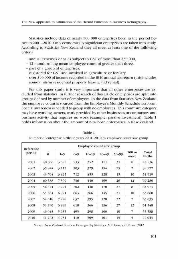
101
The New Approach to Estimation of the Hazard Function in Business Demography...
Statistics include data of nearly 500 000 enterprises born in the period be-tween 2001–2010. Only economically significant enterprises are taken into study. According to Statistics New Zealand they all meet at least one of the following criteria:
-annual expenses or sales subject to GST of more than $30 000,-12-month rolling mean employee count of greater than three,-part of a group of enterprises,-registered for GST and involved in agriculture or forestry, -over $40,000 of income recorded in the IR10 annual tax return (this includes
some units in residential property leasing and rental).
For this paper study, it is very important that all other enterprises are ex-cluded from statistics. In further research of this article enterprises are split into groups defined by number of employees. In the data from Statistics New Zealand the employee count is sourced from the Employer’s Monthly Schedule tax form. Special awareness is needed to group with no employees. This count size category may have working owners, work provided by other businesses or contractors and business activity that requires no work (example: passive investment). Table 1 holds information about the amount of new born enterprises in New Zealand.
table 1
Number of enterprise births in years 2001–2010 by employee count size group.
reference period
employee count size group
0 1–5 6–9 10–19 20–49 50–99100 or more
total births
2001 40 066 3 575 533 352 171 31 8 44 736
2002 35 844 3 115 503 329 154 25 7 39 977
2003 43 704 6 895 712 455 128 15 10 51 919
2004 60 588 7 309 736 440 169 26 12 69 280
2005 56 424 7 294 702 448 170 27 8 65 073
2006 55 464 6 991 663 366 145 21 10 63 660
2007 54 618 7 228 637 395 128 22 7 63 035
2008 53 390 6 999 618 366 136 27 12 61 548
2009 49 043 5 635 495 298 100 10 7 55 588
2010 41 272 4 931 410 309 101 15 5 47 043
Source: New Zealand Business Demography Statistics: At February 2011 and 2012
102
Paweł Zając
Only about 0.1% of all new born enterprises have more than 50 employees. The Monte Carlo simulation of such a small group of individuals most probably would generate high errors and would lead to false implications. That’s the main reason why the author decided to focus on enterprises with less than 50 employees, actually that group is known in literature as small and medium establishments (SAMEs). In this paper all enterprises from SAMEs are segregated to clusters with 0, 1–5, 6–9, 10–19 and 20–49 employees.
3. Non parametric analysis
The problem addressed by this paper is to conduct research on the “life-time” of enterprises. In classical non-parametric approaches researchers work on a group of n enterprises. Moreover, T1, ..., Tn are positive independent and identically distributed variables and they represent time between the birth and death of each enterprise (lifetime). The following notation is used:
– cumulative distribution function:
F t Prob T ti( ) = ≤( ) (1)
– density function:
f tdF t
dt( ) = ( )
(2)
– survival function:
S t F t Prob T ti( ) = − ( ) = >1 ( ) (3)
– hazard function:
h tf tS t
( ) = ( )( )
(4)
In practice F(t) represents the probability that enterprise will die until time t, the survival function S(t) is the probability of survival past time t. In this paper study is made on discrete (annual) dataset thus as by f(t) we understand the prob-ability of death at the time t. Although, the most often conditional probability is requested, probability that an enterprise will die at time t, under the condition that it still exists in t – 1 is called the hazard function h(t). The hazard function is the ratio of density and survival function.
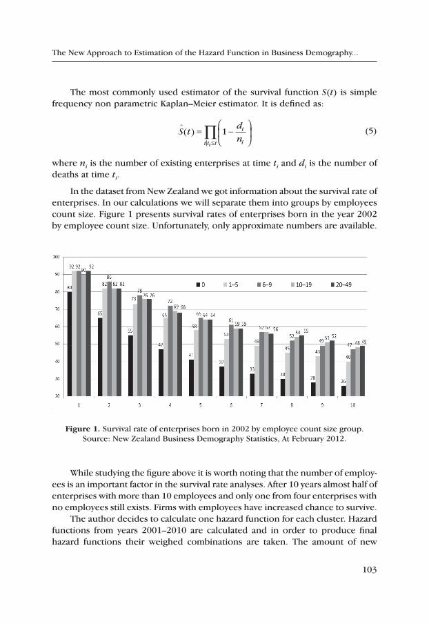
103
The New Approach to Estimation of the Hazard Function in Business Demography...
The most commonly used estimator of the survival function S(t) is simple frequency non parametric Kaplan–Meier estimator. It is defined as:
S tdni t t
i
ii
^( )
|
= −
≤∏ 1 (5)
where ni is the number of existing enterprises at time ti and di is the number of deaths at time ti.
In the dataset from New Zealand we got information about the survival rate of enterprises. In our calculations we will separate them into groups by employees count size. Figure 1 presents survival rates of enterprises born in the year 2002 by employee count size. Unfortunately, only approximate numbers are available.
Figure 1. Survival rate of enterprises born in 2002 by employee count size group. Source: New Zealand Business Demography Statistics, At February 2012.
While studying the figure above it is worth noting that the number of employ-ees is an important factor in the survival rate analyses. After 10 years almost half of enterprises with more than 10 employees and only one from four enterprises with no employees still exists. Firms with employees have increased chance to survive.
The author decides to calculate one hazard function for each cluster. Hazard functions from years 2001–2010 are calculated and in order to produce final hazard functions their weighed combinations are taken. The amount of new
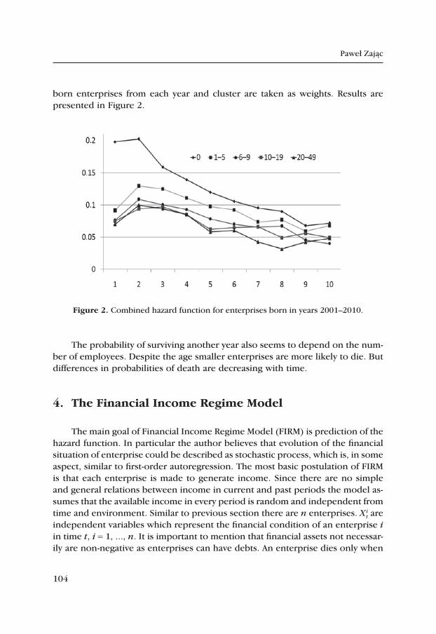
104
Paweł Zając
born enterprises from each year and cluster are taken as weights. Results are presented in Figure 2.
Figure 2. Combined hazard function for enterprises born in years 2001–2010.
The probability of surviving another year also seems to depend on the num-ber of employees. Despite the age smaller enterprises are more likely to die. But differences in probabilities of death are decreasing with time.
4. the Financial income regime Model
The main goal of Financial Income Regime Model (FIRM) is prediction of the hazard function. In particular the author believes that evolution of the financial situation of enterprise could be described as stochastic process, which is, in some aspect, similar to first-order autoregression. The most basic postulation of FIRM is that each enterprise is made to generate income. Since there are no simple and general relations between income in current and past periods the model as-sumes that the available income in every period is random and independent from time and environment. Similar to previous section there are n enterprises. Xi
t are independent variables which represent the financial condition of an enterprise i in time t, i = 1, ..., n. It is important to mention that financial assets not necessar-ily are non-negative as enterprises can have debts. An enterprise dies only when
105
The New Approach to Estimation of the Hazard Function in Business Demography...
certain level of debt is reached. The financial condition of an enterprise can be expressed using recursive algorithm:
X
X X X
X X X
i
ti
ti
ti
ti
ti
ti
ti
ti
0
1 1
1 1
0
0
0
== + ≥= + <
− −
− −
a eb e
,
,
when
when
(6)
with
e m sti N~ , .2( ) (7)
As t we understand time expressed with positive integer values. The model above contains four indicators a, b, m, s. The parameter a represents the sav-ings, of an enterprise, this parameter is used in a situation when a firm has some financial reserve, and describes what part of that reserve would be kept to the next time period. On the other hand, the parameter b can be described as infor-mation how enterprises handle their debts. Two regimes are separated according to the financial situation of a firm, change in regime depends only on financial conditions in the most recent time period. Although, the recursive structure of the model implies that Xi
t depends on the full history. Parameters m and s are mean and standard deviation of random income in a single time period. They are taken as constant and independent from time. The construction of definition (6) implies that Xi
t behave like a random walk with two additional leverages. Even though, it is a simplification zero seems to be the natural starting point for the financial state of a new born enterprise. In order to make the model as easy as possible we name the level of debts that kills the enterprise as -1. That means that when Xi
t < -1, the enterprise dies.
5. Simulations
In this section a Monte Carlo simulation is applied to the recursive formula (6). In simulation the author works with 250000 independent enterprises. More-over, for each enterprise there is generated and set a series of random values Zi
t from standard normal distribution using random number generator implied in R-program as function rnorm(). Starting value for financial condition Xi
t for each enterprise is set to zero. The values of random incomes ei
t are obtained from Zit
using formula:
e m sti
tiZ= +( ) ⋅ . (8)
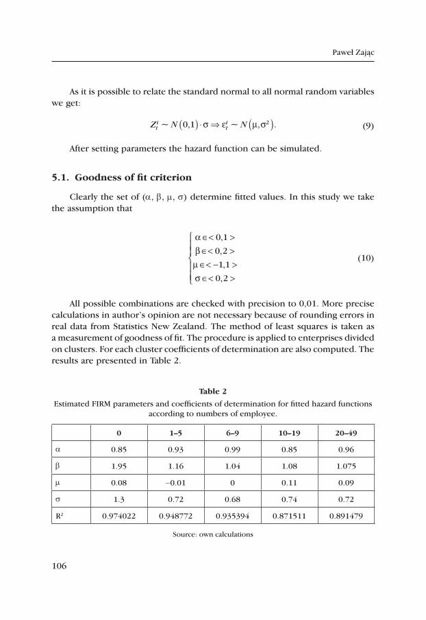
106
Paweł Zając
As it is possible to relate the standard normal to all normal random variables we get:
Z N Nti
ti~ , ~ , .0 1 2( ) ⋅ ⇒ ( )s e m s (9)
After setting parameters the hazard function can be simulated.
5.1. Goodness of fit criterion
Clearly the set of (a, b, m, s) determine fitted values. In this study we take the assumption that
abms
∈< >∈< >∈< − >∈< >
0 1
0 2
1 1
0 2
,
,
,
,
(10)
All possible combinations are checked with precision to 0,01. More precise calculations in author’s opinion are not necessary because of rounding errors in real data from Statistics New Zealand. The method of least squares is taken as a measurement of goodness of fit. The procedure is applied to enterprises divided on clusters. For each cluster coefficients of determination are also computed. The results are presented in Table 2.
table 2
Estimated FIRM parameters and coefficients of determination for fitted hazard functions according to numbers of employee.
0 1–5 6–9 10–19 20–49
a 0.85 0.93 0.99 0.85 0.96
b 1.95 1.16 1.04 1.08 1.075
m 0.08 -0.01 0 0.11 0.09
s 1.3 0.72 0.68 0.74 0.72
R2 0.974022 0.948772 0.935394 0.871511 0.891479
Source: own calculations
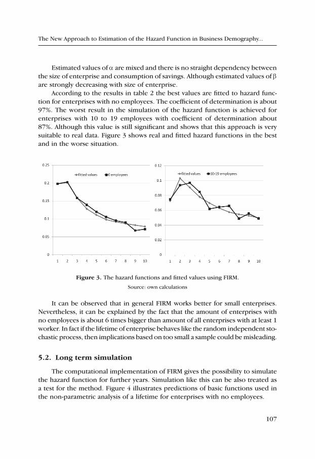
107
The New Approach to Estimation of the Hazard Function in Business Demography...
Estimated values of a are mixed and there is no straight dependency between the size of enterprise and consumption of savings. Although estimated values of b are strongly decreasing with size of enterprise.
According to the results in table 2 the best values are fitted to hazard func-tion for enterprises with no employees. The coefficient of determination is about 97%. The worst result in the simulation of the hazard function is achieved for enterprises with 10 to 19 employees with coefficient of determination about 87%. Although this value is still significant and shows that this approach is very suitable to real data. Figure 3 shows real and fitted hazard functions in the best and in the worse situation.
Figure 3. The hazard functions and fitted values using FIRM.
Source: own calculations
It can be observed that in general FIRM works better for small enterprises. Nevertheless, it can be explained by the fact that the amount of enterprises with no employees is about 6 times bigger than amount of all enterprises with at least 1 worker. In fact if the lifetime of enterprise behaves like the random independent sto-chastic process, then implications based on too small a sample could be misleading.
5.2. Long term simulation
The computational implementation of FIRM gives the possibility to simulate the hazard function for further years. Simulation like this can be also treated as a test for the method. Figure 4 illustrates predictions of basic functions used in the non-parametric analysis of a lifetime for enterprises with no employees.
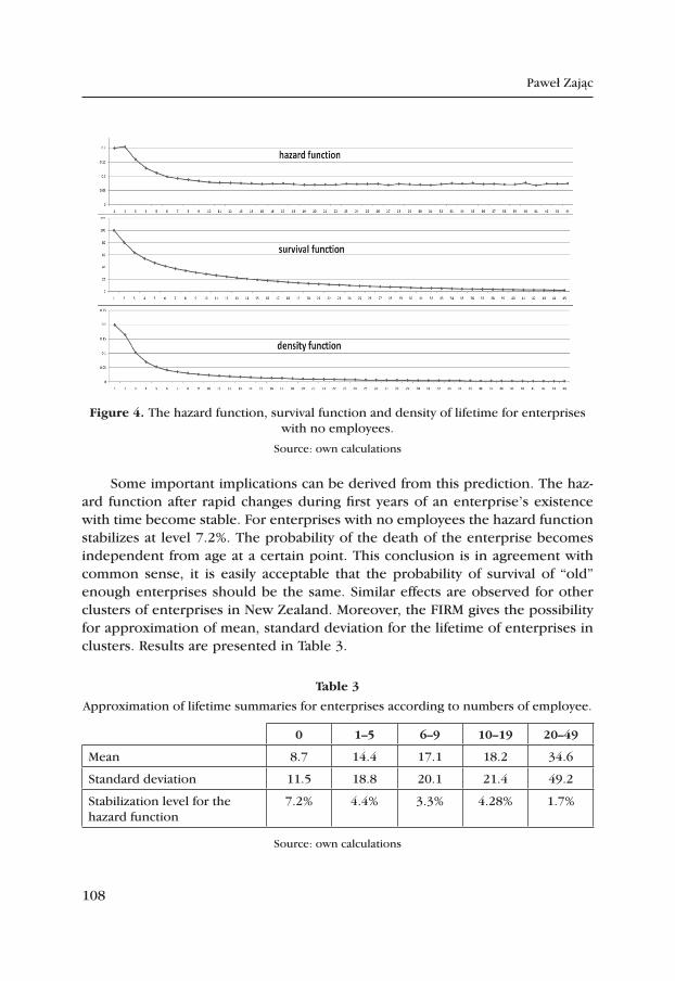
108
Paweł Zając
Figure 4. The hazard function, survival function and density of lifetime for enterprises with no employees.
Source: own calculations
Some important implications can be derived from this prediction. The haz-ard function after rapid changes during first years of an enterprise’s existence with time become stable. For enterprises with no employees the hazard function stabilizes at level 7.2%. The probability of the death of the enterprise becomes independent from age at a certain point. This conclusion is in agreement with common sense, it is easily acceptable that the probability of survival of “old” enough enterprises should be the same. Similar effects are observed for other clusters of enterprises in New Zealand. Moreover, the FIRM gives the possibility for approximation of mean, standard deviation for the lifetime of enterprises in clusters. Results are presented in Table 3.
table 3
Approximation of lifetime summaries for enterprises according to numbers of employee.
0 1–5 6–9 10–19 20–49
Mean 8.7 14.4 17.1 18.2 34.6
Standard deviation 11.5 18.8 20.1 21.4 49.2
Stabilization level for the hazard function
7.2% 4.4% 3.3% 4.28% 1.7%
Source: own calculations
109
The New Approach to Estimation of the Hazard Function in Business Demography...
Nevertheless, the probability of death of enterprises becomes stable with time, it can be observed that large enterprises are much less likely to die.
6. conclusions
The Simulation study confirms that the FIRM can be used as a tool to esti-mate the hazard function for new born enterprises. Evaluated parameters and implications from the model are in agreement with economic theory. The em-pirical results confirm that the size of an enterprise measured by the number of employees is a very important determinant of the probability of survival. Bigger firms usually can survive longer then small units. Moreover, the study indicates that the probability of death of the enterprise is decreases with age and finally after about 15 years becomes constant in time.
More research is needed to investigate the implicit formula of the hazard function based on the theoretical distribution of the stochastic process of Xi
t. Some of results of this study could be used by policy-makers to help small and
medium establishments. Acceptance that firms’ yearly income is random implies that enterprises should have some financial help from government when they experience market turbulence. It would have direct impact on a firm’s survival. Thanks to that help a lot of enterprises could get back to business with new experiences and in future pay back received help. This suggest that not only re-cently popular policies designed to promote new enterprises are important. The promotion of new firms should be accompanied by a system which helps already existing enterprises in reducing unemployment and aiming at economic growth.
references
[1] Acs Z., Audretsch D., Small Firms and Entrepreneurship: An East-West Per-spective, Cambridge University Press, 1993.
[2] Acs Z., Armington C., The Impact of Geographic Differences in Human Capital on Service Firm formation Rates, “Journal of Urban Economics” 2004, vol. 56, pp. 244–278.
[3] Agarwal R., Audretsch D.B., Does Entry Size Matter?: The Impact of the Life Cycle and Technology on Firm Survival, “Journal of Industrial Economics” 2001, vol. 49, pp. 21–43.
[4] Angelini P., Generale A., On the Evolution of Firm Size Distributions, “Ameri-can Economic Review” 2008, vol. 98(1), pp. 426–438.
[5] Astebro T., Bernhardt I., The Winner’s Curse of Human Capital, “Small Busi-ness Economics” 2005, vol. 24, pp. 63–78.
Paweł Zając
[6] Audretsch D.B., Mahmoon T., New Firm Survival: New Results Using a Hazard Function, “Review of Economics and Statistics” 1995, Vol. 77(1), pp. 97–103.
[7] Caves R.E., Industrial organization and new findings on the turnover and mobility of firms, “Journal of Economic Literature” 1998, vol. 36(4), pp. 1947–1982.
[8] Foster L., Haltinwager J.C., Krizan C.J., Aggregate Productivity Growth. Les-sons from Microeconomic Evidence, in: New Developments in Productivity Analysis, University of Chicago Press 2001, pp. 303–372.
[9] Geroski P., What do we Know About Entry, “International Journal of Indus-trial Organization” 1995, vol. 13(4), pp. 413–614.
[10] Gilbert B.A., McDougall P.P., Audretsch D.B., New Venture Growth: A review and extension, “Journal of Management” 2006, vol. 32, pp. 926–950.
[11] Gurgul H., Zając P., The dynamic model of birth and death of enterprises, “Statistics in Transition: new series” 2011, vol. 12, pp. 381–400.
[12] Jovanovic B., MacDonald G.M., The life cycle of a competitive industry, “Journal of Political Economy” 1994, vol. 102, pp. 322–347.
[13] Lin P., Huang D., Technological Regimes and Firm Survival: Evidence Across Sectors and Over Time, “Small Business Economics” 2008, vol. 30, pp. 175–186.
[14] López-Garcia P., Puente S., Business Demography in Spain: Determinants of Firm Survival, “Documentos de Trabajo” 2006, vol. 608, Banco de España.
[15] Mata J., Portugal P., Guimaraes P., The Survival of New Plants: Start-up Conditions and Post-entry Evolution, “International Journal of Industrial Organization” 1995, vol. 13(4), pp. 459–481.
[16] New Zealand Business Demography Statistics: At February 2012, Statistics New Zealand Tatauranga Aotearoa, 2012.
[17] Nunes A., Sarmento E., Business Demography Dynamics In Portugal: A Non--Parametric Survival Analysis, GEE Papers 0022, Gabinete de Estratégia e Estudos, Ministério da Economia e da Inovação, Lisbon 2010.
[18] Schumpeter J.A., Theory of Economic Development, published in 1934, Harvard Economic Studies, Cambridge 1912.
[19] van Praag C.M., Business Survival and Success of Young Small Business Owners, “Small Business Economics” 2003, vol. 21(1), pp. 1–17.
[20] Wagner J., The post-entry performance of new small firms in German manu-facturing industries, “The Journal of Industrial Economics” 1994, vol. 42(2), pp. 141–154.
[21] Wicker A.W., King J.C., Employment, ownership and survival in micro busi-ness: a study of new retail and service establishments, “Small Business Economic” 1989, vol. 1, pp. 137–152.
111
SUMMArieS
Joanna Duda: the role of bank credits in investment financing of the small and medium‑sized enterprise sector in poland Managerial Economics 2013, No. 13
Keywords: bank credit, innovations, sources of financing, SME, investment
Innovativeness of enterprises is largely dependent on their ability to obtain investment capital. Problems encountered by the SME sector when trying to obtain bank credits are commonly mentioned, therefore this paper attempts to evaluate the role of bank credits in financing in-vestment activities of Polish SMEs on the basis of available literature and empirical research. To this end, sources of financing were analysed, focusing in particular on crediting offered to small and medium-sized enterprises, costs and terms of obtaining credits are presented in reference to the structure of actual investments.
Henryk Gurgul, Roland Mestel, Robert Syrek: the testing of causal Stock re‑turns‑trading Volume Dependencies with the Aid of copulas Managerial Economics 2013, No. 13JEL classification: G15, G17
Keywords: intraday data, realized volatility, trading volume, dynamic interrelations, copulas
This paper is concerned with a dependence analysis of returns, return volatility and trading volume for five companies listed on the Vienna Stock Exchange. Taking into account the high frequency data for these companies, tests based on a comparison of Bernstein copula densities using the Hellinger distance were conducted. It is worth noting that these tests can be used in general settings since there is no restriction on the dimension of the data. The parameter which must be set up for the testing procedure is a bandwidth. It is necessary for estimation of the nonparametric copula. The paper presents some patterns of causal relationships between stock returns, realized volatility and expected and unexpected trading volume. There is linear causality running from realized volatility to expected trading volume, and a lack of nonlinear dependence in the opposite direction. The authors detected strong linear and nonlinear cau-sality from stock returns to expected trading volume. Therefore, a knowledge of past stock returns can improve forecasts of expected trading volume. They did not find causality running in the opposite direction.
Henryk Gurgul, Artur Machno, Roland Mestel: Modeling of returns and trading Volume by regime Switching copulas Managerial Economics 2013, No. 13JEL classification: G15, G17
Keywords: stock return volatility, trading volume, interdependency, regime switching copulas
The structure of links between realized volatility and trading volume can be reflected by regime switching copulas. The estimation by means of copula based regime switching models delivered

112
Summaries
results concerning the interdependencies between realized return volatility and trading volume of selected companies listed in ATX. A copula in the first regime was chosen as an asymmetric copula with positive lower and upper tail dependencies. Conversely, Gaussian copula in the second regime is a symmetric copula and variables linked with it are tail independent. For all analyzed stocks the probability of being at the first regime appeared to be vitally greater than being at the second regime. This result suggest that there is considerable dependence between realized volatility and daily volume in extreme values. The results suggest that interdependen-cies between realized volatility and trading volume do not probably depend on the size but rather on the branch of a company.
Henryk Gurgul, Marcin Suder: Modeling of Withdrawals from Selected AtMs of the “euronet” Network Managerial Economics 2013, No. 13
Keywords: ATMs, withdrawals, replenishment scheduling, SARIMA modeling
This paper deals with the problem of withdrawals from Automated Teller Machines (ATMs), using daily data for selected ATMs installed by the Euronet network in the Polish provinces of Małopolska and Podkarpacie for the period from January 2008 to March 2012. The main aim of this paper is an estimation of the proper econometric models for withdrawals time series and attempt to forecast future demand on cash flow in ATMs in respect to their localization. This is necessary to establish a replenishment schedule. The results of computations suggest that models built on the basis of SARIMA methodology are useful tools for an modeling daily withdrawals time series. This kind of model can be applied independently of the localization of an ATM. The exercises for ex post data imply ex post forecast errors under 20%. This size of forecast errors is lower than the bias of actual replenishment scheduling.
Katarzyna Liczmańska, Agnieszka M. Wiśniewska: A Strong Brand as a Determi‑nant of purchase the case of Sectors, where Advertising in Mass Media is Banned – on the example of the polish Spirits Sector Managerial Econom-ics 2013, No. 13
Keywords: brand strength, instruments of competing, purchasing decisions, ban on advertising
The purpose of the paper is the assessment of the significance of a strong brand in the pro-cess of competing for clients as well as in the clients’ decision making processes in a situation where advertising in mass media is almost completely banned. The paper presents results of two complementary studies. The first study was carried out by means of personal interviews on a trial group of 1501 individual respondents in 2007 in Poland. The second study was carried out using personal or Internet questionnaires on a trial group of 16 companies producing or importing spirits. The collected material showed that clients pointed to a strong brand as the key factor influencing their choice of top market alcohols. All representatives of producers see the need for building strong brands and declare having such brands in their offer. Building strong product brands is possible even in sectors in which mass media advertising is prohibited or for some reason cannot be used. The conceptual model proposed by the authors suggests what should be taken into account when creating a strong brand in sectors where adverting may not be used for this purpose.
Summaries
Paweł Zając: the New Approach to estimation of the Hazard Function in Business Demography on example of Data from New Zealand Managerial Economics 2013, No. 13
Keywords: business demography, birth and death of enterprise, hazard function, Monte Carlo simulation, prediction
The author presents the new methodology for the estimation of the hazard function for the new born enterprises’ survival rate called FIRM. The methodology is based on construction of a stochastic process and is examined in the Monte Carlo simulation study with real data. The dataset is provided by Statistics New Zealand and contains all enterprises born in period between 2001–2010. Enterprises are divided in clusters according to the number of employees and for each cluster individual simulations are made. Achieved coefficients of determination in clusters are around 90%. The author finds substantial differences in survival probability according to employee count size in the company. Simulations done in this study allow to estimate mean and standard deviation of life duration for enterprises and prediction of the hazard function for each cluster.


115
StreSZcZeNiA
Joanna Duda: rola kredytów bankowych w finansowaniu działalności inwe‑stycyjnej polskiego sektora MSp Managerial Economics 2013, No. 13
Słowa kluczowe: kredyt bankowy, innowacje, sektor MSP, źródła finansowania, inwestycje
Innowacyjność przedsiębiorstw jest w dużym stopniu zależna od możliwości pozyskania kapita-łów na inwestycje. Powszechnie mówi się o problemach pozyskania kredytów bankowych przez sektor MSP, dlatego też w niniejszym artykule na podstawie badań literaturowych i empirycznych podjęto próbę oceny roli kredytów bankowych w finansowaniu działalności inwestycyjnej pol-skich MSP. W tym celu dokonano analizy źródeł finansowania ze szczególnym uwzględnieniem oferty kredytowej skierowanej przez banki do małych i średnich przedsiębiorstw, przedstawiono koszty i warunki uzyskania kredytów oraz odniesiono je do struktury realizowanych inwestycji.
Henryk Gurgul, Roland Mestel, Robert Syrek: testowanie zależności przyczy‑nowych pomiędzy stopami zwrotu a wielkością obrotów za pomocą kopul Managerial Economics 2013, No. 13Klasyfikacja JEL: G15, G17
Słowa kluczowe: dane intraday, zmienność zrealizowana, wielkość obrotów, zależności dynamiczne, kopule
W artykule przeprowadzono analizę zależności pomiędzy stopami zwrotu, ich zmiennością oraz wielkością obrotów pięciu spółek notowanych na Wiedeńskiej Giełdzie Papierów Wartościo-wych. Wykorzystując dane wysokiej częstotliwości, przeprowadzono testy, wykorzystując kopule Bernsteina oraz odległość Hellingera. Warto zauważyć, że testy te mogą być zastosowane dla dowolnej liczby zmiennych. Jedynym parametrem, który musi określić badacz, jest parametr określający dokładność oszacowania nieparametrycznych gęstości kopul. W pracy zaprezento-wano pewne wzory zależności przyczynowych pomiędzy stopami zwrotu, zmiennością oraz oczekiwanym i nieoczekiwanym wolumenem. Wykazano, że istnieje zależność przyczynowa od zmienności zrealizowanej do oczekiwanego wolumenu i brak takiej zależności w odwrotnym kierunku. Wykryto silną zależność przyczynową liniową oraz nieliniową od stóp zwrotu do ocze-kiwanego wolumenu. Oznacza to, że znajomość historycznych stóp zwrotu może być pomocna w prognozowaniu oczekiwanego wolumenu. Nie wykryto zależności w kierunku przeciwnym.
Henryk Gurgul, Artur Machno, Roland Mestel: Modelowanie stóp zwrotu i wiel‑kości obrotów za pomocą kopuł przełącznikowych Managerial Economics 2013, No. 13Klasyfikacja JEL: G15, G17
Słowa kluczowe: zmienność stóp zwrotu, wielkość obrotów, zależność, kopule przełącznikowe
Struktura zależności pomiędzy zmiennością zrealizowaną a wielkością obrotów może być oddana za pomocą kopul przełącznikowych. Estymacja za pomocą kopul przełącznikowych dostarczyła

116
Streszczenia
wyniki dotyczące zależności pomiędzy zmiennością zrealizowaną a wielkością obrotów wybra-nych spółek notowanych w indeksie ATX na Giełdzie Wiedeńskiej. W pierwszym reżimie została wybrana asymetryczna kopula z dodatnimi zależnościami w ogonach. Natomiast w drugim reżimie została wybrana kopula Gaussa, która jest symetryczna oraz łączy zmienne niezależne w ogonach. W przypadku wszystkich badanych spółek prawdopodobieństwo przebywania w pierwszym reżimie okazało się znacznie większe. Taki wynik sugeruje, iż na rynku istnieje zależność dla ekstremalnych wartości między zmiennością zrealizowaną a wielkością obrotów. Uzyskane wyniki sugerują, że na silę zależności nie ma prawdopodobnie wpływu wielkość spółki, a istotnym czynnikiem jest tu przypuszczalnie branża, do której spółka przynależy.
Henryk Gurgul, Marcin Suder: Modelowanie wypłat z wybranych bankomatów sieci „euronet” Managerial Economics 2013, No. 13
Słowa kluczowe: bankomaty, wypłaty, schematy napełniania gotówką, modelowanie SARIMA
W artykule został rozważony problem modelowania i prognozowania dziennych wypłat z ban-komatów sieci „Euronet” zainstalowanych w województwie małopolskim oraz podkarpackim w okresie od stycznia 2008 do marca 2012. Głównym celem tego artykułu była estymacja modeli szeregów czasowych wypłat z wybranych bankomatów i próba prognozy zapotrzebowania na gotówkę w zależności od ich lokalizacji. Takie badania są niezbędne w celu ustalenia schematu napełniania bankomatów gotówką. Wyniki badań sugerują, że modele bazujące na liniowym modelu ARIMA uwzględniającym efekty sezonowe są użytecznymi narzędziami modelowania szeregów czasowych dziennych wypłat z bankomatów. Okazało się, że ten typ modeli może być stosowany niezależnie od lokalizacji bankomatów. Prognozy ex post są obarczone błędami poniżej 20%. Jest to błąd niższy niż błędy występujące przy stosowaniu obecnych schematów napełniania bankomatów gotówką.
Katarzyna Liczmańska, Agnieszka M. Wiśniewska: Silna marka jako determinan‑ta zakupu w sektorach objętych zakazem reklamy publicznej – przykład polskiego sektora alkoholi wysokoprocentowych Managerial Economics 2013, No. 13
Słowa kluczowe: siła marki, instrumenty konkurowania, decyzje zakupowe, zakaz reklamy
Zadaniem artykułu była ocena znaczenia silnej marki w procesach konkurowania o klienta, a także w procesach decyzyjnych konsumentów w sytuacji, gdy reklama jest prawnie zabro-niona. Ostatecznie autorki proponują model budowania silnej marki w zbiorze determinant zakupowych w sytuacji zakazu stosowania reklamy. W artykule przedstawiono wyniki dwóch uzupełniających się badań. Pierwsze zostało zrealizowane metodą wywiadu osobistego na próbie 1500 respondentów indywidualnych w Polsce w roku 2007, natomiast drugie przeprowadzono metodą ankiety bezpośredniej lub internetowej na próbie 16 przedsiębiorstw produkujących bądź importujących alkohole wysokoprocentowe. Zebrany materiał pozwolił stwierdzić, iż konsumenci jako główny czynnik wyboru w przypadku alkoholi z wyższych półek cenowych wskazują silną markę, a wszyscy przedstawiciele producentów zauważają potrzebę budowania silnych marek oraz deklarują, że mają takie w swojej ofercie. W artykule dowiedziono, że w sektorach, w któ-rych obowiązuje zakaz reklamy masowej, lub z jakichś powodów reklama taka nie może być stosowana, budowanie silnych marek produktowych jest możliwe. Proponowany przez autorki model sugeruje, na co zwrócić uwagę przy tworzeniu silnej marki w sektorach, w których nie można w tym celu wykorzystać reklamy.

Streszczenia
Paweł Zając: Nowe spojrzenie na estymację funkcji hazardu dla prawdo‑podobieństwa przeżycia przedsiębiorstw na przykładzie danych z Nowej Zelandii Managerial Economics 2013, No. 13
Słowa kluczowe: demografia biznesu, narodziny i śmierć przedsiębiorstwa, funkcja hazardu, symulacje Monte Carlo, predykcja
Autor przedstawia nową metodologię o nazwie FIRM służącą do estymacji funkcji hazardu dla prawdopodobieństwa przeżycia nowo powstałych przedsiębiorstw. Metodologia opiera się na konstrukcji procesu stochastycznego i jest przetestowana z wykorzystaniem symulacji Monte Carlo na rzeczywistych danych. Dane pochodzą z Nowej Zelandii i zawierają informację na temat przedsiębiorstw powstałych w tym kraju w latach 2001–2010. Przedsiębiorstwa podzielone są na grupy w zależności od liczby pracowników, symulacje prowadzone są dla każdej grupy. Współ-czynniki determinacji osiągnięte w procesie symulacji oscylują w okolicy 90%. Autor zauważa znaczące różnice w prawdopodobieństwie przeżycia przedsiębiorstw w zależności od wielkości firmy mierzonej liczbą pracowników. Przeprowadzone symulacje pozwoliły na estymację średniej i odchylenia standardowego długości życia przedsiębiorstw oraz predykcję nieznanych wartości funkcji hazardu w każdej z grup.


119
instruction for authors
Please send your article with a short summary in English and Polish (printed and electronic versions) to the following addresses:
Akademia Górniczo-HutniczaWydział Zarządzaniadr Joanna Dudaul. Gramatyka 1030–067 Kraków
Articles which are to be published in Managerial Economics should be pre-pared according to the following guidelines.
Length of the paper should not exceed 22 typed pages (figures and tables included).
The running text of the body of the paper should be followed by figures and tables. Tables, figures and photographs should be placed in the text after the first reference to them.
Title page should include a footnote, giving the author’s affiliation.
Figures must be prepared in a form suitable for direct reproduction. Digital artwork at least 300 dpi resolution is accepted. Photographs, on glossy paper (9 by 13 cm or larger), should display sharp contrast. Figures, tables and photo-graphs should be numbered according to their reference in text.
For computer edited texts, please include a disc with a text file, giving the edi-tor programme used (preferably Word or WordPerfect). Illustrations should be edited in CorelDraw (*.CDR), DrawPerfect (*.WPG) or in any other vector graph-ics form e.g. HPGL, Encapsulated PostScript (*.EPS), Computer Graphics Metafile *.CGM) or bitmaps (*.TIF, *.PCX).

Instruction for authors
Mathematical equation within the text should be written in separate lines, numbered consecutively (numbers within round brackets) on the right-hand side. Greek characters must be written out clearly. Reference to literature within the text should be given in square brackets.
Papers should be submitted in two copies.
Summery (of 15–20 lines) and keywords should be submitted in both Polish and English on separate sheet containing the name of the author, title of the paper with the heading “Summary”.
Authors using Word are requested to employ, as far as possible, text form of mathematical symbols leaving graphic form for the equations longer than single line.
The author should use the numbering style of referencing. References to literature within the text should be given in square brackets. Lists of references should be written in alphabetical-chronological order.
Information about the journal and the deadlines for submitting articles for next issues as well as the tempate according to which the papers should be pre-pared are presented at
www.zarz.agh.edu.pl/Czasopisma wydziałowe/Ekonomia Menedżerskahttp://tinyurl.com/ly68a6

121
informacje dla autorów artykułów
Artykuł z krótkim streszczeniem w języku angielskim i polskim prosimy nadsyłać w wersji wydrukowanej oraz elektronicznej na adresy:
Akademia Górniczo-HutniczaWydział Zarządzaniadr Joanna Dudaul. Gramatyka 1030–067 Kraków
Artykuły przeznaczone do druku w czasopiśmie Ekonomia Menedżerska powinny być opracowane zgodnie z poniższymi wytycznymi.
Objętość nie powinna przekraczać 1 arkusza wydawniczego wraz z rysunkami i tabelami.
Tekst powinien być pisany w sposób ciągły. Tabele, rysunki, fotografie należy umieszczać w tekście po pierwszym powołaniu. Na pierwszych stronach artykułów należy zamieścić afiliacje w formie przypisu z odsyłaczem gwiazdkowym u dołu kolumny: Instytucja, Miasto.
Rysunki powinny być dostarczone w formatach umożliwiających ich edycję (grafika wektorowa), ewentualnie w postaci bitmap o rozdzielczości nie mniejszej niż 300 dpi. W rysunkach i tablicach należy unikać dużego zagęszczenia elementów. Fotografie muszą być kontrastowe, o wymiarach 9 × 13 cm lub większym. Rysunki, tabele i fotografie powinny być opisane numerami, pod którymi znajdują się w tekście. Rysunki i fotografie powinny być dostarczone w postaci oddzielnych plików.
Wzory matematyczne muszą znajdować się w oddzielnych wierszach tekstu, a numery wzorów powinny być umieszczone z prawej strony w nawiasach ( ). Litery greckie powinny być pisane pismem prostym w odróżnieniu od zmiennych,

Informacje dla autorów artykułów
które należy składać kursywą. Autorzy przygotowujący teksty przy użyciu Worda proszeni są o używanie – w miarę możliwości – tekstowego trybu zapisu znaków matematycznych i symboli i pozostawienie trybu graficznego do zapisywania wzorów dwu- i więcejwierszowych, pierwiastków itp.
Powołania w tekście na literaturę należy ująć w nawiasy [], a spis literatury zamieścić na końcu artykułu ułożony alfabetycznie.
Artykuł należy złożyć w dwóch egzemplarzach. Drugi egzemplarz przeznac-zony jest dla recenzenta.
Streszczenie artykułu powinno mieć objętość 15–20 wierszy i powinno być sporządzone w języku polskim i angielskim; powinno zawierać również słowa kluczowe w języku polskim i angielskim. Wersje językowe muszą znajdować się na oddzielnych kartkach, zawierających ponadto imię i nazwisko autora, tytuł artykułu i umieszczony na górze napis „Streszczenie”.
Informacje o czasopiśmie i terminach składania artykułów do kolejnych nume-rów oraz szablon, zgodnie z którym należy przygotować teksty, są zamieszczone na:
www.zarz.agh.edu.pl/Czasopisma wydziałowe/Ekonomia Menedżerskahttp://tinyurl.com/ly68a6

Double blind peer review procedure
1. In order to assess a quality of submitted publication the Editorial Board consults at least two outside referees which are recognized experts in the specific field.
2. At least one of the referees must represent a foreign institution (other than the home institution of each author).
3. The journal uses double blind peer review policy, i.e. neither the author nor the referee knows the identity of the other.
4. Only written referee reports are considered (journal does not accept face--to-face or phone-call-based reports). Each report should clearly express in reviewers form (referees are kindly requested to fill the review form which can be found in “For reviewers” section) the referee’s final recommenda-tion (i.e. whether the article should be accepted for publication, revised or rejected).
5. The names of the referees of particular articles are classified.6. Once a year the journal publishes the complete list of referees.
