Managing and Modeling Time-series Geoscience Data in GIS

LARRY ZHANG

eMap Division, Saudi Aramco

West Park 1, Dhahran 31311, Saudi Arabia

Email: zhang.huaisu@aramco.com

Abstract

Many oil and mining companies are increasingly trying to leverage the power of

GIS to more coherently manage spatial data and to make cross-discipline spatial

data readily available to their users, because up to 70 percent of G&G data is

spatially-enabled and time-associated. In order for geoscientists to able to use

the powerful and extensible GIS environment for making use of massive GIS

data widely available for G&G projects, G&G geodata (including the time-series

data) are highly required to spatially enable them in GIS through using spatial

engines with open standards and data models like ArcSDE, PPDM, or

OpenSpirit, which is critical for successfully modeling dynamic time-series

geodata in GIS.

The paper briefly reviews some popular techniques how to integrate and map

geodata in GIS, and then mainly focus on how to accurately manage and model

time-series geodata such as time and dynamic groundwater levels in order to

reduce risk of land management and exploration projects, when dealing with

spatially-associated time-series geodata.

Key Words: time-series spatial geodata, OpenSpirit, PPDM

2

Reviews of Geoscience Applications in GIS

Many oil companies are increasingly trying to leverage the power of GIS to more

coherently manage spatial data and to make cross-discipline spatial data readily

available to their E&P users.

It is common for geosciences’ professionals to internally apply for digital GIS 2D

surface geologic mapping through using ESRI geodatabase and extending ESRI

geoscience model 1 with high quality DEM, satellite and aircraft images to identify

subtle relationships often overlooked by previous geological exploration, for

example, shaded relief maps, or 3D regular grids, which are draped with satellite

imagery or thematic maps (Figure 1a, 1b). GIS solutions to geoscience problems

were mainly restricted to representation techniques of static surface mapping and

simple 3D geometrical features for mapping surface geology without considering

dynamic change over time (Figure 2).

Figure 1a Draped Satellite Image Figure 1b Draped Surface Geology Map

3

Figure 2 Geological Mapping Representing Complicated Surface Units in GIS

Because geological, geophysical and hydrological (G&G) data have traditionally

been managed and modeled in E&P 2, 3 databases (Finder, GeoFrame, Petrel,

OpenWorks, Discovery) or other geosciences database (EarthWorks, acQuire,

Surpac), most of oil companies that have deployed GIS to their E&P users face

several common challenges:

• How to manage time in spatial projects?

• How to internally manage and model complicated G&G data (wellbore,

well locations, 2D and 3D seismic locations, profile, cross-section, and

geologic fault and horizon data) in GIS?

• How to get the G&G spatial data into the GIS and keep it current with the

ever-changing contents of their G&G project data stores?

• How to motivate geoscientists and engineers to leverage the GIS in their

day-to-day work when most of their time is spent using dedicated

geologic, geophysical, or engineering technical applications?

So, the first problem in GIS for modeling spatial change over time consists in the

attribution of time to each time node.

4

The second problem for managing G&G data consists in the attribution of the

elevation value to each vertex and node of linear elements. In addition, 3D

geological solid bodies (geological horizon, altitude of bedding, thrust, strike-slip,

normal fault, etc) was too complex to be managed in GIS. Obviously, more

complex 3D subsurface geological bodies and structures could not be easily

edited (moved, cut, glued) in GIS. The combination of surfaces also could not

lead to the construction of discrete regions (faults divided), to which properties

can be assigned. Furthermore, topographic and geological surfaces can not be

used for the creation of irregular grids where discrete properties can be

introduced.

However, with rapid development of GIS with open standards and powerfully

extensible capabilities (supporting raster catalogs), managing spatial change in

large coverage over time becomes straightforward in GIS. Also, with more and

more GIS systems supporting OpenSpirit 4 and G&G standards like PPDM 5 and

POSC 6, GIS implementation of managing subsurface 3D data (well, well logs,

seismic survey) becomes a breakthrough for internally managing, geo-

processing, and modeling spatially-associated dynamic geosciences’ data,

including time-series data, in GIS.

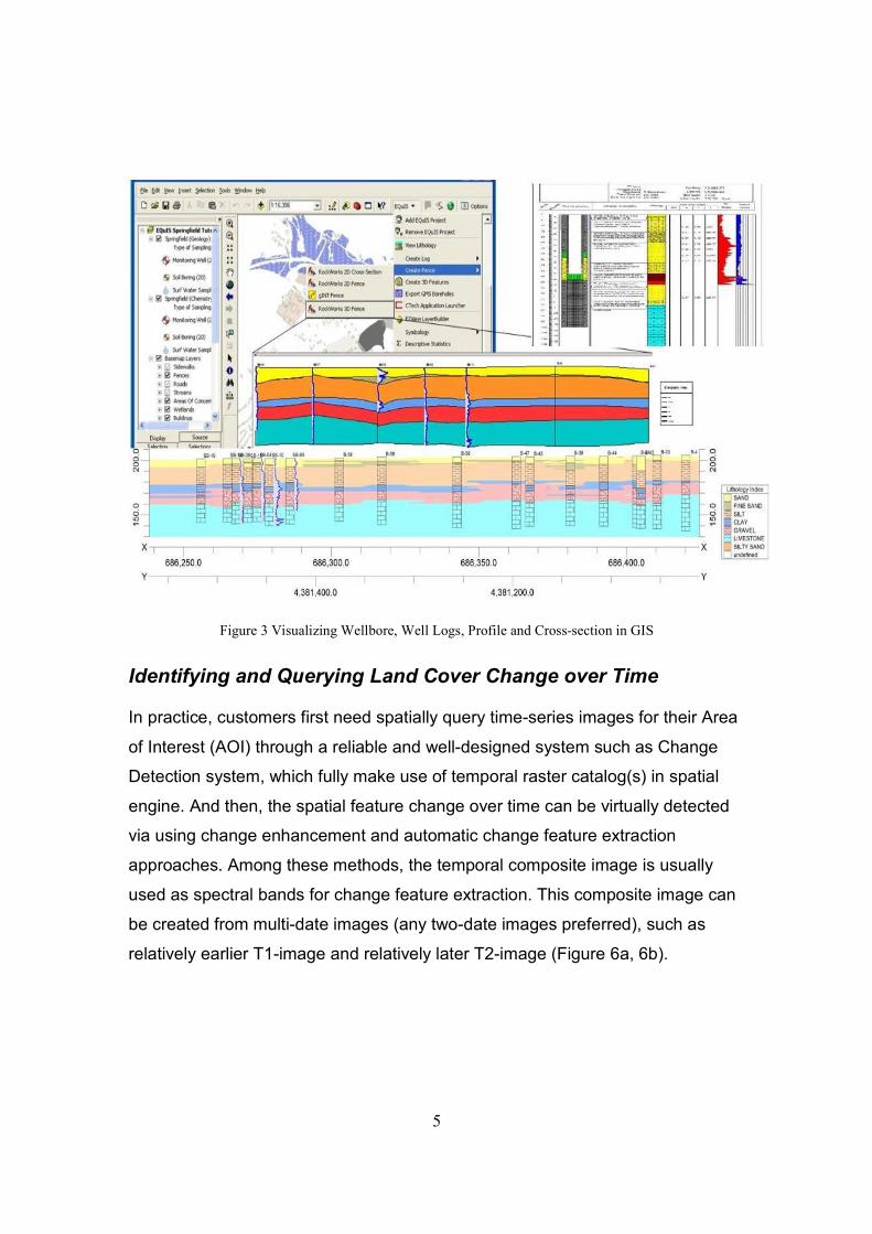
In fact, GIS can easily be interoperated and connected with external G&G or

other geosciences databases (fully managing subsurface 3D bodies and 3D

models) through using the customized extension, shapefile, or OpenSpirit

modules in order either to assure the quality of G&G geodata through using

powerful GIS spatial-query capabilities, accurate mapping, and real-time well

positioning with GPS, or to do solid 3D geomodeling and interpretation with

seismic horizons and well picks (Figure 3).

5

Figure 3 Visualizing Wellbore, Well Logs, Profile and Cross-section in GIS

Identifying and Querying Land Cover Change over Time

In practice, customers first need spatially query time-series images for their Area

of Interest (AOI) through a reliable and well-designed system such as Change

Detection system, which fully make use of temporal raster catalog(s) in spatial

engine. And then, the spatial feature change over time can be virtually detected

via using change enhancement and automatic change feature extraction

approaches. Among these methods, the temporal composite image is usually

used as spectral bands for change feature extraction. This composite image can

be created from multi-date images (any two-date images preferred), such as

relatively earlier T1-image and relatively later T2-image (Figure 6a, 6b).

6

Figure 6a Imagery of 2004 (T1) Figure 6b Imagery of 2005 (T2)

With either pixel-based or object-oriented classification in remote sensing, its

cost increases with the number of spectral bands in multispectral space. For

classifiers like the parallelepiped and minimum distance procedures, this is linear

increase with bands; however, for maximum likehood classification (most

preferred in the procedures), the cost increases with bands is quadratic.

Therefore it is sensible economically to ensure that no more bands than

necessary are utilized, that is, band selection, before performing a classification.

In addition, it is worth to realize that random band selection can not be performed

indiscriminately. The method must be devised that allow the relative worth of

bands accessed in a rigorous way. In our Change Detection system, temporal

spatial change is efficiently enhanced by integrating two temporal images into a

color composite, which consists of band 1 (Red) from band 1 in T2-image and

band 2 (Green) & band 3 (Blue) from band 2 & 3 in T1-image. From the

composite image, most real emerging objects can be easily identifying in red

color, and disappearing objects are in cyan color. With this temporal composite

image, both emerging objects and disappeared objects can be segmented and

extracted through using either automatic object-oriented classification in remote

sensing or manually digitizing in GIS.

7

It is worth to note that some grass lands and deciduous forests are also in red

color. In fact, they change seasonally, and not real feature change annually. In

practice, customers want to discriminate them from real change (Figure 7).

Figure 7 Emerging Objects in Red Color and Disappeared Objects in Cyan

Finally, for customers to conveniently query spatial change, geocoding spatial

change over time is a very important process for this kind of change detecting

system to monitor large areas across whole nation. So, temporal feature classes

of spatial change can be used as a reference for geocoding process. Geocoding

spatial change fully uses well-defined temporal change table schema in

geodatabase so that it can be updated at any time without affecting client uses.

Modeling 3D Geological Structures over Time

In order to thoroughly understand the framework of the subsurface structures and

the geological evolution over time in the prospect lease, geoscientists explore

many approaches in GIS to model and visualize the geological structures and

horizons over time with drillholes and geophysical data.

8

The simpler geological 3D model can be easily developed in GIS (X.

Devleeschouwer & F. Pouriel, 2005). The drillhole database is imported into GIS.

In 3D module, each drillhole is represented as a stick (letter A on the right). The

interpolation method (Kriging, IDW, Spline, and NN) allows modeling of the roof

for each geological layer, identified by specific colors, such as blue for the

Quaternary (letter B on the right). The picture in the lower right corner shows the

topographic map (1:10,000) draped on the digital terrain model (Figure 4).

Figure 4 Display 3D Geological Structures in GIS

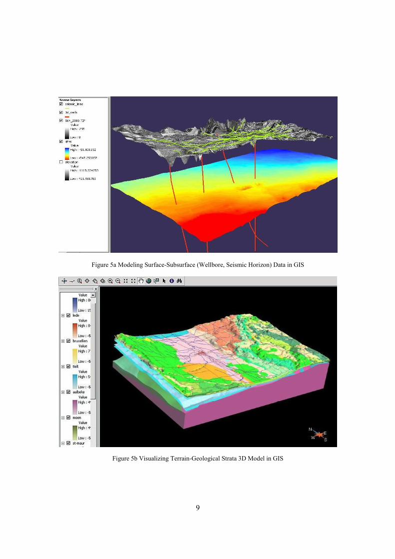
More complex geological evolution over time and geological strata models also

can be managed in GIS, which can be combined with wellbore, seismic, or

gravitational surveying data (Figure 5a, 5b). In the figure 5a, the seismic layer,

which is rendered from red color to blue, can be interpreted as time-based

horizon changes. It is worth to realize that the profile or triangular survey

(wellbore) and profiles (seismic survey) data can be interpolated with Kriging or

other methods for display and verifying well picks.

9

Figure 5a Modeling Surface-Subsurface (Wellbore, Seismic Horizon) Data in GIS

Figure 5b Visualizing Terrain-Geological Strata 3D Model in GIS

10

Managing and Modeling Groundwater Level Change over Time

In many environmental and engineering contexts, hydrological staffs need to

study regional groundwater level change over time from monitor wells. The main

difficulty with managing thousands of hourly or daily raw groundwater level

measurements from a monitor well, which is downloaded from dataloggers

(comma-separated text files, Figure 8), is the tedious process of quality control

for screening out bad data because this monitor well might be interfered from

either its own pumpage or a nearby well. Traditionally, graphing data in MS Excel

can be visualized, but can not be physically manipulated from the graph. When a

bad data value occurred in the graph, the hydrological technicians were required

to visually match errant water level values from the graph with the corresponding

value in the table. The users have to potentially scroll through the entire data

table to select the appreciate record to flag. This lengthy and tedious nature of

the QA/QC procedures in such a case often results in less than timely data

management.

Figure 8Raw Datalogger Data, Depth Measurements as Bold

A Groundwater Level Record Manager extension for ArcGIS can be developed to

easily analyze and spatially manage continuous time-series groundwater level

records, which were measured from monitor wells or their own pumpages, in

order to screen out bad data records for quality assurance (QA).

The procedure can be divided into three processes. First, the datalogger data

(comma-delimited text files) were imported into a temporary Access database

11

table. And then, the records in this table can be expressed in Cartesian space as

point event features. To produce a hydrograph in Cartesian map space, each

measurement (date/hour) is the X coordinate, and the depth-to-water is the Y

coordinate. The point event features, representing individual water level records,

can be identified, queried, rendered, updated, edited, or selected dynamically

between ArcMap and the temporary table for QA/QC (Figure 9).

Figure 9 Queried Pumping Water Level Events Rendered as Red (Bad Data) in GIS

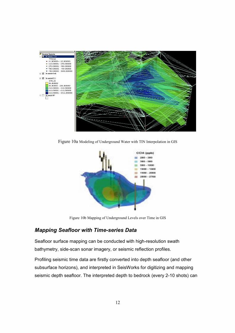
Finally, the cleaned ground water level record table in the temporary Access

database can be uploaded into enterprise underground water level database for

hydrologists to do further visualize and model groundwater surface change over

time with proper TIN (Delaunay triangulation) interpolation and ArcHydro 7 data

model in GIS through using a number of monitor wells in 3D (Figure 10a, 10b).

12

Figure 10a Modeling of Underground Water with TIN Interpolation in GIS

Figure 10b Mapping of Underground Levels over Time in GIS

Mapping Seafloor with Time-series Data

Seafloor surface mapping can be conducted with high-resolution swath

bathymetry, side-scan sonar imagery, or seismic reflection profiles.

Profiling seismic time data are firstly converted into depth seafloor (and other

subsurface horizons), and interpreted in SeisWorks for digitizing and mapping

seismic depth seafloor. The interpreted depth to bedrock (every 2-10 shots) can

13

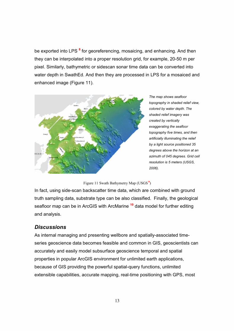
be exported into LPS 8 for georeferencing, mosaicing, and enhancing. And then

they can be interpolated into a proper resolution grid, for example, 20-50 m per

pixel. Similarly, bathymetric or sidescan sonar time data can be converted into

water depth in SwathEd. And then they are processed in LPS for a mosaiced and

enhanced image (Figure 11).

The map shows seafloor

topography in shaded relief view,

colored by water depth. The

shaded relief imagery was

created by vertically

exaggerating the seafloor

topography five times, and then

artificially illuminating the relief

by a light source positioned 35

degrees above the horizon at an

azimuth of 045 degrees. Grid cell

resolution is 5 meters (USGS,

2006).

Figure 11 Swath Bathymetry Map (USGS 9)

In fact, using side-scan backscatter time data, which are combined with ground

truth sampling data, substrate type can be also classified. Finally, the geological

seafloor map can be in ArcGIS with ArcMarine 10 data model for further editing

and analysis.

Discussions

As internal managing and presenting wellbore and spatially-associated time-

series geoscience data becomes feasible and common in GIS, geoscientists can

accurately and easily model subsurface geoscience temporal and spatial

properties in popular ArcGIS environment for unlimited earth applications,

because of GIS providing the powerful spatial-query functions, unlimited

extensible capabilities, accurate mapping, real-time positioning with GPS, most

14

surface data widely available in GIS formats, and delivering G&G /GIS analysis

over Internet. However, it does not mean that the techniques in GIS will

eventually take over G&G techniques in E&P or mining systems for managing

geodata and modeling earth. Inversely, most subsurface geodata and models are

still only available in E&P database or other geosciences database. Obviously, it

is strongly necessary for geoscientists and GIS professionals to efficiently work

together on the integration and interoperation solution for very complicated geo-

modeling applications and accurate surface-subsurface QA/QC processes. And

also, through right integration and proper interoperation, geoscientists will be

able more quickly to locate the geodata they need through, which will improve its

efficiency and productivity at both national-wide and global-wide levels.

References

1. Geosciences data model, 2005, ESRI

2. OpenWorks’ Geodata Management Manual, SeisWorks’ Training Manual,

StratWorks’ Training Manual, and Integrated Workflows in SeisWorks and

StratWorks, 1998, Landmark Graphics Corp.

3. Z-Map plus’ Workflows, Z-Map plus’ User Guide, and Z-Map plus’ Training

Manual, 2004, Landmark Graphics Corp.

4. OpenSpirit 2.9 & 3.0 User’s Guide, http://www.openspirit.com/products.html

5. PPDM 3.6 & 3.7, PPDM Lite 1.0 (the Public Petroleum Data Model),

www.ppdm.org

6. POSC 2.2 (the Petrotechnical Open Standards Consortium),

http://www.posc.org/

7. ArcHydro data model, www.crwr.utxas.edu/giswr/hydro

8. Leica Photogrammetry Suite 9 – AutoSync, Terrain Editor Tour Guide, and

Automatic Terrain Extraction User’s Guide, 2005

9. USGS, http://woodshole.er.usgs.gov/pubs/of2005-1293/

10. ArcMarine data model, http://dusk2.geo.orst.edu/djl/arcgis/