Managing Earnings at Asset Light

3PLs

The Route to Profit Maximization

1

Lean Transit – Greg W Stephens

Info@leantransit.com 904 333-4469

Discussion Objectives

2

The 3PL business environment

Characteristics of Profit Maximization for 3PLs

Profit Maximization and relationship to:

Market Segmentation

Process Control

Lean Processes

Constraints and implementation

3PL Business Environment

3

A virtually perfect competitive business model.

Pre-tax earnings for 6 public 3PLs: 1-11% of revenue with

median at 4.8%. High performers – new markets

High variable cost to revenue: 70%+ not uncommon.

No long-term excess profits

Average efficiency firms improve to levels of high performers or go

out of business (e.g. TL carriers post 1980)

High performers become more efficient or expand into markets

Over time those market expansions and efficiencies are duplicated by

competitors.

Profit Maximization

4

Key output of profit maximization strategy for asset light firms

variable cost that correlates closely to revenue.

Processes that are on target with minimum variation

$-

$1.0

$2.0

$3.0

$4.0

$5.0

$6.0

$7.0

$8.0

Pd 1Pd 2Pd 3Pd 4Pd 5Pd 6Pd 7Pd 8Pd 9 Pd10

Pd11

Pd12

Net Revenue

Variable Cost

$-

$1.0

$2.0

$3.0

$4.0

$5.0

$6.0

$7.0

$8.0

$9.0

$10.0

Pd 1Pd 2Pd 3Pd 4Pd 5Pd 6Pd 7Pd 8Pd 9 Pd10

Pd11

Pd12

Net Revenue

Variable Cost

Two actual asset light transport companies: left side firm more stable

and higher pre-tax income and higher revenue to variable cost ratio.

Profit Maximization Tools and Techniques

5

Market Segmentation:

Segment portfolio into components that have similar

characteristics

Some version typically done at 3PLs

Examples include: Big Box, Grocery, Durables, Short Term

Consumables, Distribution Centers, Ocean Carriers

Weakness tends to be in using averages and comparisons to

budget, prior year, etc. to measure performance

A more useful way is to view the business in terms of it’s

contribution, volume, etc. (variability over time and to

process performance specs)

Traffic with a Narrow Distribution is Under

Control. Focus on out-of-control Traffic

6

0

10

20

30

40

50

60

$50 $70 $90 $110 $120 $130 $150 $170 $180 $210 $380 $480 $580

Mar-

May V

olu

me

Contribution/Unit

Atlanta-Miami: Electronics

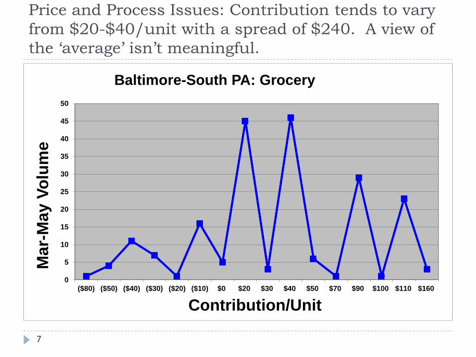
Price and Process Issues: Contribution tends to vary

from $20-$40/unit with a spread of $240. A view of

the ‘average’ isn’t meaningful.

7

0

5

10

15

20

25

30

35

40

45

50

($80) ($50) ($40) ($30) ($20) ($10) $0 $20 $30 $40 $50 $70 $90 $100 $110 $160

Mar-

May V

olu

me

Contribution/Unit

Baltimore-South PA: Grocery

Contribution Average is not meaningful. Must look at

the profile over time and identify key drivers.

8

0

2

4

6

8

10

12

(340) (150) (40) (30) (20) (10) 20 30 40 60 70 80 90 100 110 150

VO

LU

ME

CONTRIBUTION/UNIT

Jacksonville - Gainesville: Perishable Foods

MOVES

This side of the distribution is

driven by non-reimbursed

driver assessorial charges.

This side of the distribution is

driven by margin on driver

assessorial charges.

Alternative Views of Business are Useful

9

Segment Traffic with similar characteristics by location and at an actionable level (Customer, O/D, Shipper, Consignee, etc.)

Repetitive vs Non-Repetitive (Ones’ and Two’s)

Focus on managing repetitive traffic with zero execution errors

Margins become price driven vs execution driven

Stable, Lost and New Traffic

How do the margins and handling characteristics of traffic change over time?

Does the New traffic in the portfolio have fundamentally different margins and characteristics of lost traffic. Eroding margins on new traffic vs lost or stable traffic often are a

result of loss of competiveness for traffic with specific characteristics

Profit Maximization: Getting Paid for What

you do

10

Provide only those services that the customer is willing

to pay for (those you are contractually obligated to

provide.

Absolutely fundamental to high performers.

Can’t afford to sell a Lexus for a Kia price.

Eliminate components of processes that do not add value

(i.e. the customer won’t pay for)

Those process components are widespread in under

performing firms.

Focus on Control of Income Driving

Processes

11

Identify, map, and evaluate important processes

Processes are the use of inputs such as land, labor, equipment, and systems to generate output.

Analytical view: business is a set of processes that generate income

In order to improve processes the following must happen:

Process is stable

Process data is normally distributed

Process capability can be measured

Change processes that are not capable of meeting specs

Design Experiments to quantify impact of process change

Use LEAN tools (TPS) to take out non-value added process components

Process Data Tends to be and Should be

Normally Distributed

12

y = 0.0197x - 2.7993

R² = 0.9822

-3

-2

-1

0

1

2

3

32 82 132 182 232 282

Z

Normality Plot: Anderson Darling Method: Chicago Big Box Retailer

An Rsquared value of

0.8 is ‘normal’. There

are statistical methods

for ‘non-normal’ data.

Process data must be “In Control”

13

For an in-control process 100% of the data falls in a band 6

SDs wide; variations are normal in the process

An out-of-control process is characterized by special cause or

external variation (employee turnover, late trains)

Process capability can’t be measured or modified until a

process is ‘in-control’.

CL 58.6

UCL 147.9

LCL -30.6

(60)

(10)

40

90

140

190

1 2 3 4 5 6 7 8 9 10 11 12 13 14 15 16 17 18 19 20 21 22 23 24 25

Co

ntr

ibu

tio

n

Date/Time/Period

Process Control Chart : Atlanta

Process capability cannot be accurately

measured for processes not in control

14

Out of control process are not stable and thus the outputs are

not predictable.

Out-of-control processes are typically caused by data quality,

organizational instability (typically field staff), external factors,

and process design itself.

CL 297.3

UCL 628.5

0

100

200

300

400

500

600

700

800

100 200 300 400 500 600 700 800 900 100011001200130014001500160017001800190020002100220023002400 100 200

Ran

ge

Date/Time/Period

Contribution Profile over 24 Hour Period

A Process Must be able to Meet Target Specs

Consistently and with Minimum Variation: The

processes at Nashville have a 30% defect rate.

15

0

5

10

15

20

25

30

35

40

45

(369) (265) (161) (57) 47 151 255 360 464 568 672 776 880 984

Nu

mb

er

Contribution per Unit - Consumer Electronics

PROCESS CAPABILITY- NASHVILLE

LSL 50 USL 500 Mean 146 Median 140 Mode 140 n 125 Cp 0.44

Cpk 0.19 CpU 0.70 CpL 0.19 Cpm 0.35 Cr 2.26 ZTarget/DZ 0.76 Pp 0.44 Ppk 0.19 PpU 0.69 PpL 0.19 Skewness 0.58 Stdev 170 Min (265) Max 880 Z Bench 0.52 % Defects 30.4% PPM 304000.00 Expected 302829.70 Sigma 2.01

The LSC and USL

are the Lower and

Upper Spec Limits.

When the spec

limit falls inside the

distribution the

process is not

capable of meeting

requirements. Out

of spec data are

‘defects’.

Tools like Regression Identify Factors Driving

Performance. These tools are just as useful for

evaluation of commercial processes.

16

Rail Term Availability SO Receipt Drive Dispatch Term Time Drive Time Consignee Queue Service Quality

-0.5 12.2 3.1 0.47 2.9 0.25 1

1.1 24.6 2.7 0.54 2.7 0 1

0.9 13.7 3.2 0.96 3.1 0 1

1.6 22.1 5.3 0.48 2.6 0 2

4.2 4.2 0.8 1.7 3.8 1.3 3

1 15.6 2.8 1.1 2.4 0 1

2 48.5 4.7 0.36 1.9 0.7 2

1.4 12.7 3.8 0.9 2.6 0.2 2

6.2 2.3 0.7 2.1 3.5 0.9 3

-0.9 21.4 3.6 1.2 3.1 1.4 1

SUMMARY OUTPUT

Regression Statistics

Multiple R 0.991

R Square 0.982 Goodness of Fit >= 0.80

Adjusted R Square 0.945

Standard Error 0.192

Observations 10

P-value

0.134

0.002 Availability at Rail Terminal Significant Variable

0.049

0.082

0.064

0.295

0.022 Consignee Queue Significant Variable

Factors Impacting Consignee Delivery Performance

By eliminating non-significant factors one at a time

all the performance driving factors are isolated

17

Rail Term Availability SO Receipt Drive Dispatch Term Time Consignee Queue Service Quality

-0.5 12.2 3.1 0.47 0.25 1

1.1 24.6 2.7 0.54 0 1

0.9 13.7 3.2 0.96 0 1

1.6 22.1 5.3 0.48 0 2

4.2 4.2 0.8 1.7 1.3 3

1 15.6 2.8 1.1 0 1

2 48.5 4.7 0.36 0.7 2

1.4 12.7 3.8 0.9 0.2 2

6.2 2.3 0.7 2.1 0.9 3

-0.9 21.4 3.6 1.2 1.4 1

SUMMARY OUTPUT

Regression Statistics

Multiple R 0.986

R Square 0.972 Goodness of Fit >= 0.80

Adjusted R Square 0.937

Standard Error 0.206

Observations 10

Independent Variable P-value

Rail Term Availability 0.001 Eliminate Non-Significant "Causes"

SO Receipt 0.033 and you now have 4 signfificant factors

Drive Dispatch 0.047 Lower P Value indicates more signficant.

Term Time 0.072

Consignee Queue 0.012

Factors Impacting Consignee Delivery Performance

Design of Experiments can be used to test

Process Changes

18

Objective: Change process inputs to optimize process

outputs

Variety of methods available: requires absolute adherence

to design of the experiment

After the experiment an algebraic equation is used to set

the optimal inputs.

Not a trivial exercise (but doable) in service businesses

dependent on multiple vendors and non-controllable

factors. Often used in supply chain applications

Difficult to communicate visually.

There are many tools available for

forecasting trends in market factors

19

Multiple Regression Analysis: Used when two or more

independent factors are involved-widely used for intermediate

term forecasting.

Nonlinear Regression: Does not assume a linear

relationship between variables-frequently used when time is

the independent variable.

Trend/Time Series Analysis: Uses linear and nonlinear

regression with time as the explanatory variable-used where

patterns vary over time.

Decomposition Analysis: Used to identify several patterns

that appear simultaneously in a time series. Also used to de-

seasonalize data.

Once processes are under control and meet customer

specifications LEAN processes are used to increase

efficiency

20

LEAN: Invented in 1950s; also called TPS (Toyota Production

System).

Core principle: Maximize customer value at minimum cost.

Used in both manufacturing and service industries.

Define value streams in business and take out every non-value

added step.

Involves development of ‘value stream’ maps

Used extensively in logistics, supply chain, and administrative

processes; often for information flow mapping and analysis

Firms also could benefit in administrative and field operations

processes.

Constraints and Implementation

21

Organization should be relatively stable

Restructuring, cutbacks, etc. create instabilities that make projects not sustainable

Organize project into maximum 8-12 week sub projects

Continually demonstrate meaningful progress

Keeps team members focused

Use project as a mechanism to grow business profitability not cut overheads

People will not cooperate if seen as a way to eliminate their job

Expert judgment required in every phase

Use Rapid Prototyping for initial development of IT components of projects

Implementation in internal IT platform required for sustainability