managing logistics flows through enterprise input...

3

Managing Logistics Flows Through Enterprise Input-Output Models

V. Albino1, A. Messeni Petruzzelli1 and O. G. Okogbaa2

1DIMeG, Politecnico di Bari, Bari, 2DIMSE, University of South Florida,

1Italy 2USA

1. Introduction

Nowadays, the management of logistics flows is becoming a crucial activity for competitiveness. In fact, globalization is changing the way in which companies organise their production and distribution activities, considerably increasing the spatial complexity of supply chains (see also Choi & Hong, 2002; Stephen, 2004). Therefore, firms have to redesign their supply chains, both global (Meixell & Gargeya, 2005) and local (Carbonara et al., 2001), in order to sustain competitiveness and to deal with the new geography of customers and suppliers (see also Hulsmann et al., 2008; Keane & Feinberg, 2008). In this economic scenario, logistics activities cannot be more considered as a derived demand, but as a key factor for achieving competitive advantage (Hesse & Rodrigue, 2004; Gunasekaran & Cheng, 2008). In fact, the reduction of transportation time and costs can lead supply chains to improve their effectiveness and efficiency. With this regard, in the literature several studies have focusing their attention on the analysis of logistics performance, providing measures and indicators, supporting managers and policy makers in the identification of logistics strategies and policies (see also Lai & Cheng, 2003; Lai et al., 2004). Furthermore, globalization has moved competition from single companies to whole supply chains, thus requiring a joint design and management of logistics flows (Xu & Beamon, 2006; Yi & Ozdamar, 2007). Therefore, in order to guarantee the integrated and effective organization of logistics services, their management and coordination is generally assigned to specific actors, namely third-party logistics (3PL) provider or logistic service provider (LSP) (e.g. Hertz & Alfredsson, 2003; Carbone & Stone, 2005; Kim et al., 2008), which constitute the interconnectedness among the different actors of the supply chain. This new generation of actors is called into being to provide a total logistics service enabling faster movement of goods, shorter turnaround time, more reliable delivery, and reducing the number of transfers. Moreover, the growing attention towards the environmental sustainability has forced organizations to manage their logistics activities evaluating the environmental effects (e.g. Jayaraman & Ross, 2003; Wang & Chandra, 2007). In fact, international trades, global activities of multinationals, and the division of labour/production are strongly increasing

Ope

n A

cces

s D

atab

ase

ww

w.in

tech

web

.org

Source: Supply Chain, The Way to Flat Organisation, Book edited by: Yanfang Huo and Fu Jia, ISBN 978-953-7619-35-0, pp. 404, December 2008, I-Tech, Vienna, Austria

www.intechopen.com

Supply Chain, The Way to Flat Organisation

34

these negative effects, which are also accentuated by the growing market share of the most energy intensive modes of transportation (truck and air1) and the relative decline of other modes (ship and rail2) (EEA, 2004). The EU White Paper on Transport Policy (CEC, 2001) recognises that transport energy consumption is increasing and that 28% of CO2 emissions are now transport-related. Carbon dioxide emissions continue to rise, as transport demand outstrips improvements in energy-related emissions. The sector with the largest projected increase in EU-15 emissions is transport. In this scenario, consumers and governments are pressing companies to re-design and carefully manage their logistics networks, in order to reduce the environmental impact of their products and processes (Thierry et al., 1995; Quariguasi Frota Neto et al., 2008). In the present paper, we propose the use of enterprise input-output (EIO) models to represent and analyse physical and monetary flows between production processes, including logistics ones. In particular, we consider networks of processes transforming inputs into outputs and located in specific geographical areas. The paper is structured as follows. In the following section, a brief review of EIO models is presented. Then, in Section 3 some possible application fields of EIO models are identified. Sections 4 and 5 describe the basic equations of EIO models and their use. In Section 6 and 7 EIO models are applied to represent and analyse transportation processes, both at an aggregate and disaggregate level, and logistics services markets, respectively. Finally, the main findings and results are summarized into discussion and conclusions (Section 8).

2. Enterprise input-output models

The input-output (IO) approach has been typically applied to analyse the structure of economic systems, in terms of flows between sectors and firms (Leontief, 1941). So doing, analysing the interdependencies among entities, economists and managers can evaluate the effect of technological and economic change at regional, national, and international level. According to the different level of analysis, IO models can be highly aggregated or disaggregated. Miller and Blair (1985) use a disaggregated level and consider the pattern of materials and energy flows amongst industry sectors, and between sectors and the final customer. A higher level of disaggregation is useful to define a model better fitting real material and energy flows. However, the drawback of working on a high level of disaggregation is represented by the lack of consistency in the input coefficients. In fact, it is sufficient that technological changes happen in a process to modify the input coefficients. On the other hand, because of the small scale, it is easy to know which technological changes are employed in one or more processes and the modifications to apply to the technical coefficients. EIO models constitute a particular set of IO models, useful to complement the managerial and financial accounting systems currently used extensively by firms (Grubbstrom & Tang, 2000; Marangoni & Fezzi, 2002; Marangoni et al., 2004). In particular, Lin and Polenske (1998) proposed a specific IO model for a steel plant, based on production processes rather than on products or branches. Similarly, Albino et al. (2002, 2003) have developed IO models for analyzing in terms of material, energy, and pollution flows the complex dynamics of

1 Air transport is growing by 6–9 % per year in both the old and new EU Member States. 2 The market shares of modes such as rail are increasing only marginally, if at all.

www.intechopen.com


35

global and local supply chains, and of industrial districts, respectively. Moreover, EIO models based on processes have been adopted to evaluate the effect of different coordination policies of freight flows on the logistics and environmental performance of an industrial district (Albino et al., 2008). At the single firm’s level the EIO model can be useful to coordinate and manage internal and external logistics flows. At the level of the whole industrial cluster the enterprise input-output model can be effective to analyse logistics flows and to support coordination policies among firms and their production processes. As in the case of industrial districts, EIO models can be applied to contexts highly characterized by the geographical dimension, such as the local and global supply chains. For better addressing the spatial dimension the EIO approach can be integrated with GIS technology, geographically referring all the inputs and outputs accounted in the models (e.g. Van der Veen & Logtmeijer, 2003; Zhan et al., 2005; Albino et al., 2007). This paper aims at investigating logistics related issues adopting EIO models. To cope with this aim, transportation is modelled as a process (or input) both at an aggregate and disaggregate level, providing the other processes with the logistics services necessary to convey products from origins to destinations. In the former, transportation is modelled as a single process (or input) that supplies all the other production processes involved in the chain. Alternatively, it can be modelled considering all the tracks representing the transportation network through which products flow to and from production processes using the disaggregate approach. These two approaches are used to pursue different system goals. In particular, the aggregate model is used to analyse the logistics flows from a managerial perspective. In fact, economic and operational performance can be evaluated. Whereas, the adoption of a disaggregated approach permits a more space-oriented analysis. Specifically by modelling all the tracks it is possible to examine issues related to traffic congestion, transportation infrastructure availability, and pollutant emissions in specific geographical areas.

3. EIO models for logistics: a framework of analysis

As stated in the previous section, EIO models are accounting and planning tools aimed at describing production process and analyzing their reciprocal interdependences. Here, we intend to shed further light on the adoption of EIO models to manage logistics flows, providing a framework that identifies their main application fields and explains their usefulness. In particular, we can consider two main perspectives under which the production processes and related logistics flows can be investigated: i) a spatial and ii) an operational perspective. In the former, the processes are described referring to their location into a specific geographical area. This approach can be effective to examine space-related issues, such as traffic congestion, pollutant emissions, transportation infrastructure, and work force

availability. In this case, the analysis is applied to the set ΠG, constituted by all the processes

πi (i=1,…,n) located in the area G. Adopting an operational perspective, goals oriented to maximize the efficiency and effectiveness of the processes belonging to a specific supply chain can be pursed. Therefore,

the application field is related to the set ΠSC, constituted by all the processes πi (i=1,…,n) belonging to the supply chain SC. Moreover, considering the logistic flows associated to the production processes, a further application can be represented by the analysis of all the

www.intechopen.com


36

flows between processes πi (i=1,…,n) managed by a specific logistic provider. Thus, the set

ΠLP, constituted by all the flows ωij (i=1,…,n and j=1,…,m) managed by a specific logistic provider LP, can be studied. These application fields are not mutually exclusive. In fact, they can be combined in order to

provide more specific and complex analysis. For instance, we can consider the set ΠG ∩ Πsc, represented by all the processes located in the area G and involved in the supply chain SC.

Then, we can describe the generic process πi belonging to this set adopting both an operational and geographical perspective. In particular, all its inputs and outputs are described taking into account the nature and their origins and destinations.

In Figure 1, the process πi is represented, identifying its main output (xi), the inputs supplied

by other processes belonging to ΠG ∩ Πsc (z1i, z2i,…, zni), the wastes and by products

produced by πi (w1, w2,…, wn), and the other primary inputs required by πi and supplied by

processes that are not included into the set to ΠG ∩ Πsc (r1, r2,…, rs).

πi

z1i

z2i

zni

r1 r2 rs

xi

w1w2 wnwk

rk

zki

Fig. 1. Inputs and outputs of the process πi.

This representation can be useful for accounting purposes, since it permits to identify the

outputs produced by the process and all the required inputs. However, in order to take into

account the spatial characteristics of inputs and outputs they have to be geographically

referred, considering their origins and destinations. All the processes belonging to ΠG ∩ Πsc

can be geo-referred as well as the flows between them.

In fact, the primary input rk can be supplied by distinct origins. Thus, we can distinguish the

input on the basis of its origins, being rkA and rkB, where A and B represent two distinct

locations. Moreover, also the main output can be delivered to different destinations. In

particular, these destinations can belong or not to the considered set of processes. In the

latter, we indicate as fi the output produced by pi and destined outside the boundary of the

system. Therefore, the main output can be distinguished on the basis of the destinations. For

instance, we can have fiC and fiD. The same consideration can be applied to wastes and by

products (wkG, wkF).

In Figure 2 the process πi is represented considering the geographical locations of inputs and outputs.

www.intechopen.com


37

πi

rkA rkB

wkE

zi1

zi2

fiC

fiD

wkF

z1i

z2i

zni

zki

z1i

z2i

zni

zki

zikzin

Fig. 2. Inputs and outputs of the process pi, distinguished by geographical locations.

Therefore, these two distinct representations permit to move from a physical and monetary description of the processes (Figure 1) to a spatial one (Figure 2).

4. EIO models and production processes: basic equations

Let us consider a set of production processes. This set can be fully described if all the interrelated processes as well as input and output flows are identified and modelled. Let Z0 be the matrix of domestic (i.e. to and from production processes within the set) intermediate deliveries, f0 is the vector of final demands (i.e. demands leaving the set), and x0 the vector of gross outputs. If n processes are distinguished, the matrix Z0 is of size n x n, and the vectors f0, and x0 are n x 1. It is assumed that each process has a single main product as its output. Each of these processes may require intermediate inputs from the other processes, but not from itself so that the entries on the main diagonal of the matrix Z0 are zero. Of course, also other inputs are required for the production. These are s primary inputs (i.e. products not produced by one of the n production processes). Next to the output of the main product, the processes also produce m by-products and waste. r0 and w0 are the primary input vector, and the by-product and waste vector of size s x 1 and m x 1, respectively. Define the intermediate coefficient matrix A as follows:

1

0 0ˆA Z x−≡

where a “hat” is used to denote a diagonal matrix. We now have:

( ) 1

0 0 0 0x Ax f I A f

−= + = −

It is possible to estimate R, the s x n matrix of primary input coefficients with element kjr

denoting the use of primary input k (1,…, s) per unit of output of product j, and W, the m x n

matrix of its output coefficients with element kjw denoting the output of by-product or

waste type k (1,…, m) per unit of output of product j. It results:

0 0r R x=

www.intechopen.com


38

0 0w W x=

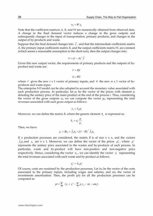
Note that the coefficient matrices A, R, and W are numerically obtained from observed data. A change in the final demand vector induces a change in the gross outputs and subsequently changes in the input of transportation, primary products, and changes in the output of by-products and waste.

Suppose that the final demand changes into f , and that the intermediate coefficients matrix

A, the primary input coefficients matrix R, and the output coefficients matrix W, are constant (which seems a reasonable assumption in the short-run), then the output changes into:

1( )x I A f−= −

Given this new output vector, the requirements of primary products and the outputs of by-product and waste are:

r Rx=

w Wx=

where r gives the new s x 1 vector of primary inputs, and w the new m x 1 vector of by-products and waste types. The enterprise I-O model can be also adopted to account the monetary value associated with each production process. In particular, let p0 be the vector of the prices with element pi

denoting the unitary price of the main product at the end of the process i. Thus, considering the vector of the gross outputs x0, we can compute the vector y0, representing the total revenues associated with each gross output as follows:

0 0 0ˆy x p=

Moreover, we can define the matrix B, where the generic element ijb is expressed as:

i

ij ij

j

pb a

p=

Then, we have: ( ) 1

0 0 0 0 0 0ˆ ˆy By f p I B f p

−= + = −

If n production processes are considered, the matrix B is of size n x n, and the vectors

0 0f̂ p and

0y are n x 1. Moreover, we can define the vector of the prices

0

wp , where w

ip

represents the unitary price associated to the wastes and by-products of each process. In

particular, waste and by-product will have non-positive and non-negative price

respectively. Hence, considering the vector 0w , we can identify the vector

0

wy representing

the total revenues associated with each waste and by-product as follows:

0 0 0ˆw wy w p=

Of course, costs are sustained by the production processes. Let in0 be the vector of the costs associated to the primary inputs, including wages and salaries, and an0 the vector of investments amortization. Then, the profit (pt) for all the production processes can be computed as:

1

( )n

w

i i j ji i ii j

pt y y p z in am=

= + − − −∑ ∑

www.intechopen.com


39

5. EIO models for a supply chain stage

In the present section, we propose a theoretical example, aimed at describing the physical and monetary flows associated with a network of production processes, not including transportation, taking into account the geographical location of inputs and outputs. For the sake of simplicity, a supply chain stage is considered. Let us consider three production processes, π1, π2, and π3, belonging to Πsc and exchanging products as shown in Figure 3.

π1

π2

π3zπ1π3

f1

r1

r2

r1

w1

w2

zπ2π3

fπ3

Fig. 3. Inputs and outputs of production processes in a supply chain stage.

Adopting the EIO models, the balance table accounting the materials flows of the supply chain stage is reported in Table 1.

Processes π1 π2 π3 f0 x0

π1 331 πππ xa

1πf 1πx

π2 332 πππ xa

2πx

π3 3πf 3πx

Primary inputs

r1 111 ππ xr 221 ππ xr

r2 332 ππ xr

Wastes and by-products

w1 111 ππ xw

w2 332 ππ xw

Table 1. Balance table for the supply chain stage in Figure 3.

As previously explained, the same type of input and output can be characterised by different origins and destinations. Let us assume that the final demand f3 is delivered to the geographical destinations A and B, the primary input r2 comes from the geographical

www.intechopen.com


40

origins C and D, and the waste w1 is destined to the geographical destinations E and F (Figure 4).

π1

π2

π3

f1

r1

r1

w1E

w2

w1F

r2Cr2D

zπ1π3

zπ2π3

fπ3A

fπ3B

Fig. 4. Inputs and outputs of production processes distinguished by geographical origins and destinations.

On the basis of this representation, it is possible to define the related balance table, reported in Table 2.

Processes π1 π2 π3 f0A f0B x0

π1 331 πππ xa

1πf 1πx

π2 332 πππ xa

2πx

π3 Af 3π Bf 3π 3πx

Primary inputs


r2C 33,2 ππ xr C

r2D 33,2 ππ xr D


w1E 11,1 ππ xw E

w1F 11,1 ππ xw F

w2 332 ππ xw


Balance tables referring to the monetary flows among processes can be similarly computed.

6. EIO models for logistics flows in a supply chain stage

The flows of materials among processes and their final outputs require to be conveyed from origins to destinations. Therefore, in order to effectively describe and analyse the network of

www.intechopen.com


41

production processes, transportation has to be considered. For the sake of simplicity, a supply chain stage is analyzed. In EIO models, transportation can be modelled as: i) a production process or ii) a primary input, which provides other processes with inputs consisting of logistics service, in terms of the distance covered to convey all main products to their destinations. In particular, the transportation system can be modelled as a single production process (T) that supplies all the other production processes involved in the supply chain stage and requires inputs such as workforce, fuel, and energy, as shown in Figure 5.

π1

π2

π3

fπ1

r1

r2

r1

w1

w2

T

zTπ1

zTπ2

r3

w1

zπ1π3

zπ2π3

zTπ3fπ3

Fig. 5. Inputs and outputs of production processes, including transportation.

Following this approach, the balance table can be represented as shown in Table 3.

Processes π1 π2 π3 T f0 x0

π1 331 πππ xa

1πf 1πx

π2 332 πππ xa

2πx

π3 3πf 3πx

T 11 ππ xaT

22 ππ xaT 33 ππ xaT Tx

Primary inputs


r2 331 ππ xr

r3 TT xr3


w1 111 ππ xw 11 xw T

w2 331 ππ xw


www.intechopen.com


42

Logistics flows can be also modelled adopting a disaggregate approach, i.e. a single transportation process can be associated to each origin and destination materials flow (Figure 6). Moreover, transportation processes can also be distinguished on the basis of the logistics flow, if materials and the trucks load capacity are different.

π1

π2

π3

r1

r2

r1

w2T1

T2

t3

ZT1π1

w1

w1

w1

r3

r3

r3

ZT2π2

fπ1

fπ3

zπ2π3

zπ1π3

ZT3π3

Fig. 6. Inputs and outputs of production processes, including transportation for each origin-destination flow.

In this case, the balance table is reported in Table 4.

Processes π1 π2 π3 T1 T2 T3 f0 x0

π1 331 πππ xa

1πf 1πx

π2 332 πππ xa

2πx

π3 3πf

3πx

T1 111 ππ xaT 1Tx

T2 222 ππ xaT

2Tx

T3 333 ππ xaT

3Tx

Primary inputs


r2 332 ππ xr

r3 113 TT xr

223 TT xr 333 TT xr


w1 111 ππ xw 111 TT xw

221 TT xw331 TT xw

w2 332 ππ xw


www.intechopen.com


43

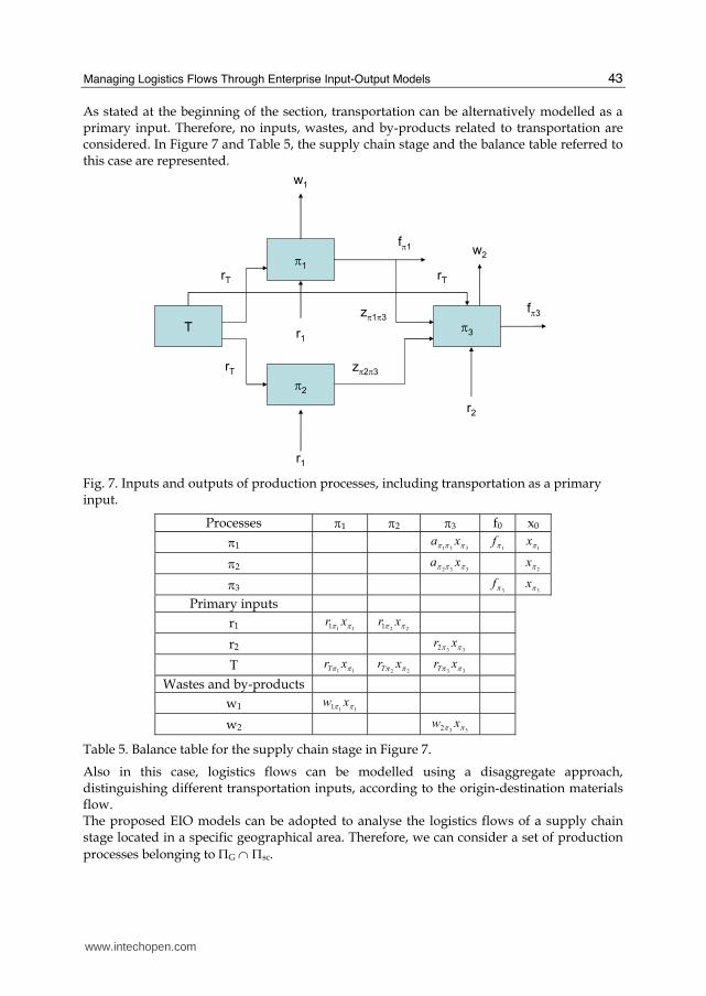
As stated at the beginning of the section, transportation can be alternatively modelled as a primary input. Therefore, no inputs, wastes, and by-products related to transportation are considered. In Figure 7 and Table 5, the supply chain stage and the balance table referred to this case are represented.

π1

π2

π3

r1

r2

r1

w1

w2

T

rT

rT zπ2π3

zπ1π3

rT

fπ1

fπ3

Fig. 7. Inputs and outputs of production processes, including transportation as a primary input.

Processes π1 π2 π3 f0 x0

π1 331 πππ xa

1πf 1πx

π2 332 πππ xa

2πx

π3 3πf 3πx

Primary inputs


r2 332 ππ xr

T 11 ππ xrT

22 ππ xrT 33 ππ xrT


w1 111 ππ xw

w2 332 ππ xw


Also in this case, logistics flows can be modelled using a disaggregate approach, distinguishing different transportation inputs, according to the origin-destination materials flow. The proposed EIO models can be adopted to analyse the logistics flows of a supply chain stage located in a specific geographical area. Therefore, we can consider a set of production

processes belonging to ΠG ∩ Πsc.

www.intechopen.com


44

However, these models are not able to make distinction about primary inputs, wastes, by-products, and outputs transportation. To make distinction, we add virtual processes located within the considered geographical area G or on its boundaries, depending on where the primary input is available (within or outside the area). Each virtual process, corresponding to a specific primary input, is characterised by geographical information about its location and it has an output that can be transported to all the production processes requiring that input. For each virtual process no inputs are allowed from the production processes.

Let us consider h virtual processes corresponding to s primary inputs from outside the

geographical system. Then, we introduce *

0Z and *

0x as the matrix of domestic intermediate

deliveries and the vector of gross outputs including the h virtual processes, respectively. If n

processes are distinguished, including transportation processes, the matrix *

0Z is of size

(n+h) x (n+h) and the vector *

0x is (n+h) x 1.

Define the intermediate coefficient matrix A* as follows:

* * 1*

0 0ˆA Z x−≡

The apex * can be extended with similar meaning to all variables as needed. The same approach can be used to model wastes and by-products transportation. Let us consider two production processes, πj and πk, two virtual processes, v1 and v2, corresponding to two primary inputs, r1 and r2, respectively, and the process T having, for the sake of simplicity, no intermediate deliveries from processes πj and πk, and no primary inputs. Moreover, each process, primary input, waste, and by-product is characterised by a single location, and no imports are considered from outside G, unless the two primary inputs. Finally, let us assume that the final demand fπk is delivered to the geographical destination A and the waste w1 is destined to the geographical destination B (Figure 8).

πj πk

v1 v2

T

zTπkzTπj

zTv2zTv1

fπkAzπjπk

w1B w1B

w1B w1B

r1r2

zv1πj zv2πk

w1B

Fig. 8. Inputs and outputs of production processes, including transportation and virtual processes.

www.intechopen.com


45

In Table 6 the balance table referred to the supply chain stage depicted in Figure 8 is reported.

Process πj πk T v1 v2 f0A x0

πj kkj

xa πππ j

xπ

πk Akfπ

kxπ

T jj

xaT ππ kk

xaT ππ Tx

v1 jjxav ππ1

1vx

v2 kk

xav ππ2

2vx

Primary inputs

r1 111 vv xr

r2 222 vv xr


w1B jj

xw B ππ,1kk

xw B ππ,1 TTB xw ,1 11,1 vvB xw22,1 vvB xw


As previously explained, the main output of process T is represented by the total distance covered by transportation means to deliver products from origins to destinations. Thus, considering the distance between the processes, as provided in Table 7, we can compute, for

instance, jT

z π as: 1

j k

jT

zz d

C

π ππ = ⋅

where C represents the transportation means’ load capacity.

From/to πj πk v1 v2

πj d1 d2 d3πk d1 d4 d5

v1 d2 d4 d6

v2 d2 d4 d6

Table 7. Distance between processes.

Moreover, the distances between the processes can be distinguished into the different paths covered to convey products, which are constituted by the track connecting the processes, as shown in Table 8.

From/to πj πk v1 v2

πj θ1-θ2 θ1-θ3 θ1-θ4πk θ2-θ1 θ2-θ3 θ2-θ4

v1 θ3-θ1 θ3-θ2 θ3-θ4

v2 θ4-θ1 θ4-θ2 θ4-θ3

Table 8. Paths covered by transportation means.

Therefore, jT

z π results:

( )1 2 1 2

j k j k j k

jT

z z zz d d d d

C C C

π π π π π ππ θ θ θ θ= + ⋅ = ⋅ + ⋅

www.intechopen.com


46

where 1dθ and

2dθ represent the lengths of the track θ1and θ2, respectively.

On the basis of these considerations, the transportation process can be modelled adopting a

disaggregate approach into l processes (k

θ , k=1,…, l), corresponding to the l tracks covered

by transportation means to deliver products. In this case, the balance table reported in Table 4 can be described as in Table 8.

Process πj πk θ1 θ2 θ3 θ4 v1 v2 f0A x0

πj kkj

xa πππ j

xπ

πk Akfπ

kxπ

θ1 jj

xa ππθ1

111 vv xaθ 1θx

θ2 jj

xa ππθ2 kkxa ππθ2

222 vv xaθ

2θx

θ3 113 vv xaθ

3θx

θ4 224 vv xaθ

4θx

v1 jj

xav ππ1 1vx

v2 kk

xav ππ2 2vx

Primary inputs

r1 111 vv xr

r2 222 vv xr


w1B jj

xw B ππ,1kk

xw B ππ,1 11,1 θθ xw B 22,1 θθ xw B 33,1 θθ xw B 44,1 θθ xw B 11,1 vvB xw22,1 vvB xw

Table 8. Balance table in the disaggregated representation of transportation processes.

Adopting the disaggregate approach, each transportation input is related to a given track

kθ (k=1,…, h). Then, each process delivering products to two or more final destinations can

be distinguished according to their final destinations, maintaining the same geographical

location. In fact, let us assume to have three production processes (π1, π2, and π3) and two

tracks (1θ and

2θ ), with the balance table reported in Table 9, where

1θ and

2θ connect π1

with π2, and π1 with π3, respectively.

π1 π2 π3 F

π1 0 12z

13z 0

π2 0 0 0 f2π3 0 0 0 f3

θ1 11t 0 0

θ2 21t 0 0

Table 9. Balance table.

www.intechopen.com


47

If f2 increases, then 12z must increase and, consequently, x1 increases. However, only

11t

must increase to permit to serve more output of π1 to π2. Then, the process p1 has to be

distinguished into p12 and p13, according to its final destinations, as shown in Table 10.

π12 π13 π2 π3 F

π12 0 0 12z 0 0

π13 0 0 0 13z 0

π2 0 0 0 0 f2

π3 0 0 0 0 f3

θ1 1,12t 0 0 0

θ2 0 2,13t 0 0

Table 10. Balance table in the case of process π1 distinguished according to its final destinations.

Now, 1,12t and

2,13t represent the distance covered by the transportation mean to convey the

output of process π1 to the process π2 through the track θ1, and the output of process π1 to

the process π3 through the track θ2, respectively.

Finally, it is important to compute and geo-refer the pollution caused by the transportation

means along the tracks. Then, let us define the waste vector 0wθ of size m x 1 and the m x h

matrix W θ of output coefficients with element kjwθ denoting the output of waste type k

(1,…,m) per unit of transportation input j.

It results:

0 0w Wθ θθ=

Then, pollution caused by transportation can be easily computed and geo-referred.

7. EIO models and logistics services markets

As stated in Section 1, logistics services are generally managed by logistics providers (3PL),

which own the key competencies and capabilities necessary to assure their effectiveness and

efficiency.

Referring to transportation services, three distinct actors can be identified: i) suppliers,

which have to deliver products to one or more customers; ii) customers, which require

products from one or more suppliers; iii) 3PL providers, which provide the transportation

service and coordinates logistics flows between suppliers and customers.

The interaction among these different actors represents what is generally defined as a

logistics services market. In particular, it can be composed by actors belonging both to the

same companies, or different and independent ones.

Adopting EIO models it is possible to describe these markets modelling each actor as a

different production process.

Let us consider three suppliers (S1, S2, and S3), two customers (C1, C2, and C3), and two

logistics providers, which are represented by two distinct transportation processes (T1, and

www.intechopen.com


48

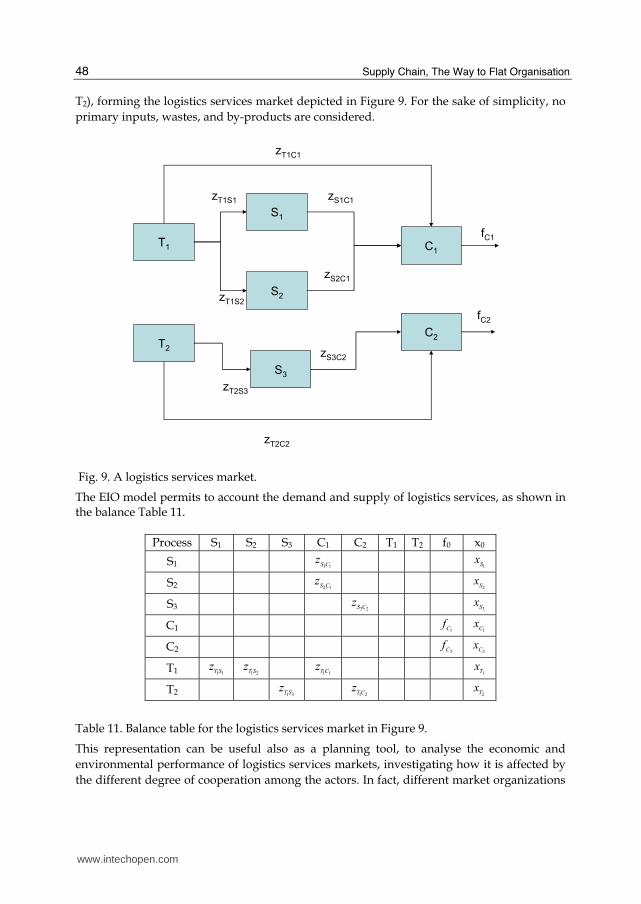
T2), forming the logistics services market depicted in Figure 9. For the sake of simplicity, no

primary inputs, wastes, and by-products are considered.

S2

S1

S3

C1

C2

T1

T2

zS1C1

zS2C1

zS3C2

fC1

fC2

zT1S1

zT1S2

zT2S3

zT2C2

zT1C1

Fig. 9. A logistics services market.

The EIO model permits to account the demand and supply of logistics services, as shown in the balance Table 11.

Process S1 S2 S3 C1 C2 T1 T2 f0 x0

S1 1 1S Cz

1Sx

S2 2 1S Cz

2Sx

S3 3 2S Cz

3Sx

C1 1Cf

1Cx

C2 2Cf

2Cx

T1 1 1T Sz

1 2T Sz

1 1T Cz

1Tx

T2 1 3T Sz

1 2T Cz

2Tx

Table 11. Balance table for the logistics services market in Figure 9.

This representation can be useful also as a planning tool, to analyse the economic and

environmental performance of logistics services markets, investigating how it is affected by

the different degree of cooperation among the actors. In fact, different market organizations

www.intechopen.com


49

can be proposed and investigated, on the basis of the collaboration degree of the actors, and

following approaches aimed at minimizing the number of trips, such in as in the case of

consolidation strategies, and at creating logistics networks specialized, for instance, by

geographical areas, types of product, and services.

8. Discussion and conclusions

The present paper has proposed the use of EIO models to describe and analyse logistics

flows to support managers and policy makers in the definition of policies for their

management and coordination. In particular, different approaches and models have been

proposed.

Two main perspectives have been used to analyse logistics flows, such as a spatial and

operational one, pursuing different goals. In fact, geo-referring the production processes

belonging to a supply chain, and their inputs and outputs, spatial-oriented analyses can be

performed in order to deal with issues related to traffic congestion, pollutant emissions,

transportation infrastructures, and work force availability. Therefore, on the basis of these

analyses policies aimed at improving the transportation sustainability and reducing its

negative impact on the environment can be identified.

Differently, the adoption of an operational framework of analysis can permit to describe

logistics flows involved in specific supply chains, or, more in detail, managed by specific

actors, in order to analyse and improve logistics economic performance. For instance,

solutions aimed at consolidating the flows and reducing the number of trips and the

transportation costs can be achieved.

Moreover, transportation has been modelled both as a process and as a primary input. The

difference between these two approaches depends on the inclusion of inputs required and

wastes produced by transportation. In fact, in the former all the transportation inputs, such

as workforce and fuel, and its pollutant emissions are considered. Therefore, this approach

can be useful for 3PL to evaluate the economic and environmental performance of their

activities. On the contrary, the modelling of transportation as a primary input can be used to

investigate its impact on the supply chains. In fact, in this case the model can be a suitable

accounting and planning tool for actors representing the demand of logistics services, in

order to analyse, for instance, how logistics affects their profit and operations.

Transportation has been also modelled at an aggregate and disaggregate level. The

aggregate level of analysis permits to investigate managerial-oriented issues, giving a

holistic view of the transportation to evaluate its global role on the supply chains’ efficiency

and effectiveness. Differently, the disaggregate approach permits a more in-depth analysis,

since it describes all the tracks covered by transportation means, thus allowing policy

makers to propose actions for the logistics management according to a social and

environmental perspective.

Finally, EIO models have been used to represent logistics service markets, in order to

account and analyse the demand and supply of transportation. This can be useful for both

logistics providers and customers to organize markets, on the basis of different criteria (e.g.

consolidation, specialization, geographical areas) and to improve their performance.

The present study contributes to extend the existing framework on logistics management,

providing a set of complete and complementary tools, based on the use of EIO models, able

www.intechopen.com


50

to analyse the problem according to different perspectives and point of views. The power of

the described methodology is strictly related to the possibility to investigate the impact of

logistics on the whole performance systems, thanks to the direct and indirect relationships

and interdependences among production processes.

Further researches should be devoted to apply the models to actual cases, in order to show

their effectiveness as both accounting and planning tools and to strength the relevance of the

proposed approach.

9. References

Albino, V., De Nicolò, M., Garavelli, A.C., Messeni Petruzzelli, A., Yazan, D.M. (2007) Rural

development and agro-energy supply chain. An application of enterprise input-

output modelling supported by GIS, 16th International Input-Output Conference, July

2-6, Istanbul, Turkey.

Albino, V., Dietzenbacher, E., Kühtz, S. (2003) Analyzing Material and Energy Flows in an

Industrial District using an Enterprise Input-Output Model, Economic Systems

Research, Vol. 15, pp. 457-480.

Albino, V., Izzo, C., Kühtz, S. (2002) Input-Output Models for the Analysis of a

Local/Global Supply Chain, International Journal of Production Economics,

Vol. 78, pp. 119-131.

Albino, V., Kuhtz, S., Messeni Petruzzelli, A., (2008) Analysing logistics flows in industrial

clusters using an enterprise input-output model, Interdisciplinary Information

Sciences, Vol. 14, pp. 1-17.

Carbonara, N., Giannoccaro, I., Pontrandolfo, P. (2001) Supply chains within industrial

districts: theoretical framework, International Journal of Production Economics, Vol.

76, pp. 159-176.

Choi, T.Y Hong, Y. (2002) Unveiling the structure of supply networks: case studies in

Honda, Acura, DaimlerChrysler, Journal of Operations Management, Vol. 20, pp.

469–493.

Commission of the European Communities (2001) European Transport Policy for 2020: Time to

Decide (Luxembourg: Office for Official Publications of the European

Communities).

European Energy Agency (2004) EEA signals 2004, A European Environment Agency Update on

Selected Issues (Copenhagen: European Energy Agency).

Grubbström, R.W., Tang, O. (2000) An Overview of Input-Output Analysis Applied

to Production-Inventory Systems, Economic Systems Research, Vol. 12, pp. 3-

25.

Gunasekaran, A., Cheng, T.C.E. (2008) Special issue on logistics: new perspectives and

challenges, Omega, Vol., 36, pp. 505-508.

Hertz S., Alfredsson M. (2003) Strategic development of third party logistics provider,

Industrial Marketing Management, Vol. 30, pp. 139-149.

Jayaraman, V., Ross, A. (2003) A simulated annealing to distribution network design

and management, European Journal of Operational Research, Vol. 144, pp. 629-645.

www.intechopen.com


51

Kim, C., Yang, K.H., Kim, J. (2008) A strategy for third-party logistics systems: a case

analysis using the blue ocean strategy, Omega, Vol. 36, pp. 522-534.

Lai, K.H., Cheng, T.C.E. (2003) A Study of the Freight Forwarding Industry in Hong

Kong, International Journal of Logistics: Research and Applications, Vol. 7, pp. 72-

84.

Lai, K.H., Ngai, E.W.T., Cheng, T.C.E. (2004) An empirical study of supply chain

performance in transport logistics, International Journal of Production Economics, Vol.

87, pp. 321-331.

Leonief, W.W. (1941) The Structure of the American Economy. Oxford University Press, New

York.

Lin, X., Polenske, K.R. (1998) Input-Output Modelling of Production Processes for

Business Management, Structural Change and Economic Dynamics, Vol. 9, pp.

205-226.

Marangoni, G., Colombo, G., Fezzi, G. (2004) Modelling Intra-Group Relationships, Economic

Systems Research, Vol. 16, pp. 85-106.

Marangoni, G., Fezzi, G. (2002) I-O for Management Control: The Case of GlaxoSmithKline,

Economic Systems Research, Vol. 14, pp. 245-256.

Meixell, M.J., Gargeya, V.B. (2005) Global supply chain design: a literature review and

critique, Transportation Research, Vol. 41, pp. 531-550.

Miller, R.E., Blair, P.D. (1985) Input Output Analysis: Foundations and Extensions. Prentice

Hall, Englewood Cliffs.

Quariguasi Frota Neto, J., Bloemhof-Ruwaard, J.M., van Nunen, J.A.E.E., van Heck, E. (2008)

Designing and evaluating sustainable logistics networks, International Journal of

Production Economics, Vol. 111, pp. 195-208.

Stephen, T. (2004) Further reflections on the supply chain complexity gap, Supply Chain

Europe, Vol. 13, pp. p. 38.

Thierry, M., Salomon, M., van Nunen, J.A.E.E., van Wassenhove, L. (1995) Strategic issues

in product recovery management, California Management Review, Vol. 37, pp. 114-

135.

Van der Veen, A., Logtmeijer, C. (2003) How vulnerable are we for flooding? A GIS approach,

(No. EUR Report 20997 EN). Office for Official Publications of the European

Communities, European Commission, Brussels.

Wang, Y., Chandra, L.S. (2007) Using e-business to enable customised logistics

sustainability, International Journal of Logistics Management, Vol. 18, pp. 402-

419.

Xu, L, Beamon, B.M. (2006) Supply chain coordination and cooperation mechanisms: an

attribute-based approach, The Journal of Supply Chain Management, Winter 2006, pp.

4-12.

Yi, W., Ozdamar, L. (2007) A dynamics logistics coordination model for evacuation and

support in disaster response activities, European Journal of Operational Research, Vol.

179, pp. 1177-1193.

www.intechopen.com


52

Zhan, G., Polenske, K.R., Ning, A. (2005) Evaluation of yellow-dust storms and

countermeasure policies in North China using regional input-output models, 15th

International Input-Output Conference, 27 June – 1 July, Beijing, P.R. of China.

www.intechopen.com

Supply Chain the Way to Flat OrganisationEdited by Julio Ponce and Adem Karahoca

ISBN 978-953-7619-35-0Hard cover, 436 pagesPublisher InTechPublished online 01, January, 2009Published in print edition January, 2009

InTech EuropeUniversity Campus STeP Ri Slavka Krautzeka 83/A 51000 Rijeka, Croatia Phone: +385 (51) 770 447 Fax: +385 (51) 686 166www.intechopen.com

InTech ChinaUnit 405, Office Block, Hotel Equatorial Shanghai No.65, Yan An Road (West), Shanghai, 200040, China

Phone: +86-21-62489820 Fax: +86-21-62489821

With the ever-increasing levels of volatility in demand and more and more turbulent market conditions, there isa growing acceptance that individual businesses can no longer compete as stand-alone entities but rather assupply chains. Supply chain management (SCM) has been both an emergent field of practice and anacademic domain to help firms satisfy customer needs more responsively with improved quality, reduction costand higher flexibility. This book discusses some of the latest development and findings addressing a number ofkey areas of aspect of supply chain management, including the application and development ICT and theRFID technique in SCM, SCM modeling and control, and number of emerging trends and issues.

How to referenceIn order to correctly reference this scholarly work, feel free to copy and paste the following:

V. Albino, A. Messeni Petruzzelli and O. G. Okogbaa (2009). Managing Logistics Flows Through EnterpriseInput-Output Models, Supply Chain the Way to Flat Organisation, Julio Ponce and Adem Karahoca (Ed.),ISBN: 978-953-7619-35-0, InTech, Available from:http://www.intechopen.com/books/supply_chain_the_way_to_flat_organisation/managing_logistics_flows_through_enterprise_input-output_models

managing logistics flows through enterprise input...

Documents