managing schema change in an heterogeneous environment
TRANSCRIPT

Managing Schema Change in anHeterogeneous Environment
by
Kajal Tilak Claypool
A Dissertation
Submitted to the Faculty
of the
WORCESTER POLYTECHNIC INSTITUTE
in Partial Fulfillment of the Requirements for the
Degree of Doctor of Philosophy
in
Computer Science
by
May 2002
APPROVED:
Prof. Elke A. RundensteinerAdvisor
Prof. Carolina RuizCommittee Member
Prof. George T. HeinemanCommittee Member
Prof. Stan ZdonikExternal Committee MemberBrown University, Providence, RI
Dr. Arnon RosenthalExternal Committee MemberMITRE Corporation, Burlington, MA
Prof. Micha HofriHead of Department

ii

iii
Abstract
“Nothing endures but change. ”
–By Heractilus
Change is inevitable even for persistent information. Effectively man-
aging change of persistent information, which includes the specification,
execution and the maintenance of any derived information, is critical and
must be addressed by all database systems. Today, for every data model
there exists a well-defined set of change primitives that can alter both the
structure (the schema) and the data. Several proposals also exist for incre-
mentally propagating a primitive change to any derived information (or
view). However, existing support is lacking in two ways. First, change
primitives as presented in literature are very limiting in terms of their ca-
pabilities allowing users to simply add or remove schema elements. More
complex types of changes such the merging or splitting of schema elements
are not supported in a principled manner. Second, algorithms for maintain-
ing derived information often do not account for the potential heterogene-
ity between the source and the target. The goal of this dissertation is to
provide solutions that address these two key issues.
The first part of this dissertation addresses the challenge of expressing

iv
a rich complex set of changes. We propose the SERF (Schema Evolution
through an Extensible, Re-usable and Flexible) framework that allows users
to perform a wide range of complex user-defined schema transformations.
Our approach combines existing schema evolution primitives using OQL
(object query language) as the glue logic. Within the context of this work,
we look at the different domains in which SERF can be applied, including
web site management. To further enrich our framework, we also investi-
gate the optimization and verification of SERF transformations.
The second part of this dissertation addresses the problem of maintain-
ing views in the face of source changes when the source and the view are
not in the same data model. With today’s increasing heterogeneity in infor-
mation structure, it is critical that maintenance of views addresses the data
model boundaries. However, view definitions that go across data models
are limited to hard-coded algorithms, thereby making it difficult to develop
general maintenance algorithms. We provide a two-step solution for this
problem. We have developed a cross algebra, that defines views such that
there is no restriction that forces the view and the source data models to be
the same. We then define update propagation algorithms that can propa-
gate changes from source to target irrespective of the exact translation and
the data models. We validate our ideas by applying them to translation and
change propagation between the XML and relational data models.

v
Acknowledgments
There are many people who have helped me in this work, either directly by
working on projects with me or indirectly by giving me vision and support.
However, above all there are three people who deserve my deepest grati-
tude: Professor Elke Rundensteiner, my husband, Mark and my Papa. As
my advisor, Elke has contributed to all levels of this thesis, from guidance
on English grammar rules to providing focus and vision for my research.
Equally important, Mark has been a pillar of strength and support. He
has been understanding of the many late nights and the many weekends I
spent away from him and our two kids. Most importantly, he has provided
motivation to persevere through the slow and difficult parts of my disser-
tation, and more importantly, helped me keep my focus on finishing when
I may have given up. He is my inspiration in more ways than one.
My father taught me how to set my sights high and how to succeed.
His motto “just work hard” did well for me during my years at school. In

vi
many ways he is the reason that I did this. So Papa, this one is for you!
I would also like to thank my mother, my brother, my two boys and my
in-laws. Akaash and Saahil, thank you for the infinite patience you showed
me when I was gone on the weekends and when I had to do my homework
before I could help you with yours! Thank you boys. Thank you Mom for
being supportive and encouraging and helping out with the kids whenever
you could. Thanks Amit for patiently listening to me whine! Last but not
the least in the family line - thanks to my parents-in-law for being very
supportive.
I would like to thank the members of my examining committee: Profes-
sors George Heineman, Carolina Ruiz, Stan Zdonik and Dr. Arnie Rosen-
thal. They helped steer the direction of my dissertation and gave me valu-
able advice along the way. Professor George Heineman provided hands-on
advising when I needed it most.
I also must thank those who long ago gave me the tools to achieve a
Ph.D. Professors John Riedl and Jaideep Srivastava, professors at Univer-
sity of Minnesota, showed me my first glimmer of research and had me
hooked.
I would like to thank my colleagues and friends in the DSRG group,
especially Li Chen, Andreas Koeller and Su Hong, for their invaluable en-
couragement and contributions to my work, and most of all for lending me
an ear when I needed it the most. Thank you.
Without the contributions of the above people, this work would never
have been completed, nor even begun.

vii
Contents
I Information Integration and Change Management 1
1 Introduction 31.1 Issues in Change Management . . . . . . . . . . . . . . . . . 31.2 Change Management - State of Art . . . . . . . . . . . . . . . 5
1.2.1 Change Specification and Execution . . . . . . . . . . 51.2.2 Managing the Effects of Change . . . . . . . . . . . . 10
1.3 Our Work . . . . . . . . . . . . . . . . . . . . . . . . . . . . . . 151.3.1 Change Specification - The SERF Framework . . . . . 161.3.2 Managing the Effects of Change - Sangam . . . . . . 20
1.4 Organization of this Dissertation . . . . . . . . . . . . . . . . 27
II SERF - An Extensible Transformation Framework 29
2 Overview 31
3 The ODMG Model and Schema Evolution 333.1 ODMG Standard: The Object Model . . . . . . . . . . . . . . 33
3.1.1 ODMG Schema Repository . . . . . . . . . . . . . . . 353.1.2 ODMG’s Object Query Language - OQL . . . . . . . 37
3.2 Evolving the ODMG Object Model . . . . . . . . . . . . . . . 393.2.1 Invariants for the ODMG Object Model . . . . . . . . 403.2.2 Taxonomy of Schema Evolution Primitives . . . . . . 42
3.3 Summary . . . . . . . . . . . . . . . . . . . . . . . . . . . . . . 50
4 The SERF Framework 514.1 Features of the Framework . . . . . . . . . . . . . . . . . . . . 514.2 Schema Transformations . . . . . . . . . . . . . . . . . . . . . 544.3 Transformation Templates . . . . . . . . . . . . . . . . . . . . 56
4.3.1 Generalization of a Transformation . . . . . . . . . . . 57

CONTENTS viii
4.3.2 Template Library . . . . . . . . . . . . . . . . . . . . . 584.3.3 SERF Template Language . . . . . . . . . . . . . . . . 594.3.4 SERF Template Instantiation and Processing . . . . . 59
4.4 Summary . . . . . . . . . . . . . . . . . . . . . . . . . . . . . . 61
5 Soundness and Consistency of SERF Templates 635.1 Soundness of Templates . . . . . . . . . . . . . . . . . . . . . 635.2 Contracts . . . . . . . . . . . . . . . . . . . . . . . . . . . . . . 665.3 Verification of ROVER Wrappers . . . . . . . . . . . . . . . . 69
5.3.1 Theorem Prover for SERF Templates . . . . . . . . . . 715.3.2 Formal Verification Process: Application to Inline Tem-
plate . . . . . . . . . . . . . . . . . . . . . . . . . . . . 735.4 Summary . . . . . . . . . . . . . . . . . . . . . . . . . . . . . . 80
6 Reducing the Runtime of SERF Templates 836.1 Optimizing the Performance of Schema Evolution Sequences 83
6.1.1 Foundations of Schema Evolution Sequence Analysis 856.1.2 The CHOP Optimization Functions . . . . . . . . . . 896.1.3 CHOP Optimization Strategy . . . . . . . . . . . . . . 966.1.4 Experimental Validation . . . . . . . . . . . . . . . . . 98
6.2 Summary . . . . . . . . . . . . . . . . . . . . . . . . . . . . . . 100
7 Design and Implementation of the OQL-SERF System 1037.1 System Architecture . . . . . . . . . . . . . . . . . . . . . . . . 1047.2 SERF Framework Modules . . . . . . . . . . . . . . . . . . . . 105
7.2.1 Template Module . . . . . . . . . . . . . . . . . . . . . 1057.2.2 Template Library . . . . . . . . . . . . . . . . . . . . . 1077.2.3 User Interface . . . . . . . . . . . . . . . . . . . . . . . 108
7.3 Summary . . . . . . . . . . . . . . . . . . . . . . . . . . . . . . 109
8 Case Study of Different Schema Transformations 1118.1 The Merge Transformation . . . . . . . . . . . . . . . . . . . . 112
8.1.1 The Merge-Union Template . . . . . . . . . . . . . . . 1138.1.2 The Merge-Difference Template . . . . . . . . . . . . . 1148.1.3 A More Complex Merge Template . . . . . . . . . . . 115
8.2 ReWEB - Applying SERF for Web Transformations . . . . . . 1178.3 Summary . . . . . . . . . . . . . . . . . . . . . . . . . . . . . . 122

CONTENTS ix
9 Related Work 1239.1 Specifying Schema Change . . . . . . . . . . . . . . . . . . . 1239.2 Optimization of Schema Evolution . . . . . . . . . . . . . . . 1279.3 Behavioral Consistency . . . . . . . . . . . . . . . . . . . . . . 1289.4 Consistency Management . . . . . . . . . . . . . . . . . . . . 1289.5 Extensible Systems . . . . . . . . . . . . . . . . . . . . . . . . 129
III Sangam - Managing Change in Heterogeneous Databases 131
10 Overview 133
11 Data Model 13711.1 Sangam Graph Model . . . . . . . . . . . . . . . . . . . . . . 13811.2 Converting Application Schemas and Data to
Sangam graphs . . . . . . . . . . . . . . . . . . . . . . . . . . 14111.2.1 XML and Sangam graphs . . . . . . . . . . . . . . . . 14111.2.2 Relational Schemas and Sangam graphs . . . . . . . 150
11.3 Summary . . . . . . . . . . . . . . . . . . . . . . . . . . . . . . 154
12 Cross Algebra 15712.1 Cross Algebra Operators . . . . . . . . . . . . . . . . . . . . . 158
12.1.1 The Cross Operator . . . . . . . . . . . . . . . . . . . . 15812.1.2 The Connect Operator . . . . . . . . . . . . . . . . . . 16012.1.3 The Smooth Operator . . . . . . . . . . . . . . . . . . 16112.1.4 The Subdivide Operator . . . . . . . . . . . . . . . . . 16212.1.5 Notation . . . . . . . . . . . . . . . . . . . . . . . . . . 165
12.2 Cross Algebra Trees . . . . . . . . . . . . . . . . . . . . . . . . 16512.2.1 Derivation Trees . . . . . . . . . . . . . . . . . . . . . 16712.2.2 Context Dependency Trees . . . . . . . . . . . . . . . 17312.2.3 Cross Algebra Graphs (CAG):
Combining Context Dependency and Derivation Trees 17912.3 Evaluating the Cross Algebra Operators -
The Physical Plan . . . . . . . . . . . . . . . . . . . . . . . . . 19312.3.1 Physical Algebra Operators . . . . . . . . . . . . . . . 19312.3.2 Evaluating a Cross Algebra Graph . . . . . . . . . . . 197
12.4 An Example . . . . . . . . . . . . . . . . . . . . . . . . . . . . 20512.4.1 The Basic Inlining . . . . . . . . . . . . . . . . . . . . . 20512.4.2 The Shared Inlining . . . . . . . . . . . . . . . . . . . 214
12.5 Summary . . . . . . . . . . . . . . . . . . . . . . . . . . . . . . 216

CONTENTS x
13 Sangam: Evaluating the Theory 21913.1 Architectural Overview of Cross Algebra Processing Engine 21913.2 Experimental Validation of Sangam . . . . . . . . . . . . . . 222
13.2.1 Loading to and Generating from Sangam Graphs . . 22413.2.2 CAG Evaluation . . . . . . . . . . . . . . . . . . . . . 22813.2.3 Summary of Experimental Results . . . . . . . . . . . 234
13.3 Summary . . . . . . . . . . . . . . . . . . . . . . . . . . . . . . 235
14 Updating the Sangam Graph 23714.1 Schema Change Operations on the Sangam Graph . . . . . . 238
14.1.1 SAG-SC: Schema Change Primitives . . . . . . . . . . 23814.1.2 Completeness of SAG-SC Operations . . . . . . . . . 24014.1.3 Correctness of Sangam graph -SC Operations . . . . . 243
14.2 Data Modification Primitives for theSangam Graph . . . . . . . . . . . . . . . . . . . . . . . . . . 244
14.3 Translation Completeness of Sangam Graph Operations . . . 24614.3.1 Translation Completeness of SAG-SC Operations . . 24614.3.2 Translation Completeness of SAG-DU Operations . . 251
14.4 Reversing the Process . . . . . . . . . . . . . . . . . . . . . . . 25914.5 Summary . . . . . . . . . . . . . . . . . . . . . . . . . . . . . . 260
15 Update Propagation 26315.1 The CAT Propagation Strategy . . . . . . . . . . . . . . . . . 264
15.1.1 Introduction . . . . . . . . . . . . . . . . . . . . . . . . 26415.1.2 Updates on CAT . . . . . . . . . . . . . . . . . . . . . 26415.1.3 Overall Propagation Strategy . . . . . . . . . . . . . . 265
15.2 Default Propagation Through the Cross Algebra Operators . 28115.2.1 Propagation Rules for SAG-SC Operations . . . . . . 28115.2.2 Propagation Rules for SAG-DU Operations . . . . . . 293
15.3 Properties of Propagation Through CAGs . . . . . . . . . . . 29715.3.1 Correctness of Propagation . . . . . . . . . . . . . . . 29715.3.2 Incremental Propagation Versus Recomputation . . . 300
15.4 Summary . . . . . . . . . . . . . . . . . . . . . . . . . . . . . . 306
16 Performance Comparison: Incremental vs Re-computation 30916.1 Incremental vs. Re-Computation . . . . . . . . . . . . . . . . 31216.2 Analyzing the Performance of Incremental Propagation . . . 313
16.2.1 The Algebra Operators . . . . . . . . . . . . . . . . . . 31416.2.2 Ident and Inline CAGs . . . . . . . . . . . . . . . . . . 323
16.3 Summary . . . . . . . . . . . . . . . . . . . . . . . . . . . . . . 328

CONTENTS xi
17 Related Work 33117.1 XML Storage . . . . . . . . . . . . . . . . . . . . . . . . . . . . 33117.2 Change Management . . . . . . . . . . . . . . . . . . . . . . . 332
17.2.1 Change Propagation within A Data Model . . . . . . 33217.2.2 Supporting Applications During Change . . . . . . . 33417.2.3 XML Update Systems . . . . . . . . . . . . . . . . . . 33617.2.4 Other Related Work. . . . . . . . . . . . . . . . . . . . 337
17.3 Schema Integration and Data Transformation . . . . . . . . . 33717.4 Data Models and Translations in the Middle Layer . . . . . . 339
17.4.1 Schema Languages . . . . . . . . . . . . . . . . . . . . 33917.4.2 Query Algebras . . . . . . . . . . . . . . . . . . . . . . 348
IV Conclusions and Future Work 361
18 Conclusions and Future Work 36318.1 Contributions of this Dissertation . . . . . . . . . . . . . . . . 364
18.1.1 Support for Complex Changes . . . . . . . . . . . . . 36418.1.2 Maintenance of Heterogeneous Views . . . . . . . . . 366
18.2 Future Directions . . . . . . . . . . . . . . . . . . . . . . . . . 36818.2.1 Optimization of Schema Evolution . . . . . . . . . . . 36818.2.2 Integrating the Cross Algebra With Existing Local Al-
gebra . . . . . . . . . . . . . . . . . . . . . . . . . . . . 37018.2.3 Inverse Update Propagation . . . . . . . . . . . . . . . 371
A DTDs Used in Experiments 373

CONTENTS xii

xiii
List of Figures
1.1 Changes in the Database Environment. . . . . . . . . . . . . 41.2 The Inline Operation. . . . . . . . . . . . . . . . . . . . . . . . 18
4.1 An Example Schema Graph for a MERGE Transformation. . 534.2 Example of the Inline Transformation. . . . . . . . . . . . . . 544.3 SERF Representation of the Inline Transformation using OQL. 544.4 Generalized Inline Template based on the Inline Transforma-
tion. . . . . . . . . . . . . . . . . . . . . . . . . . . . . . . . . . 584.5 The BNF for a SERF Template. . . . . . . . . . . . . . . . . . . 604.6 Steps for the Execution of a Template . . . . . . . . . . . . . . 61
5.1 Preconditions for Delete-Class Primitive in Contractual Form. 685.2 Postconditions for the Delete-Class Primitive Template. We
assume here that the meta-dictionary information such asPe(Cx) are available until the template is done executing. . . 68
5.3 Inline ROVER Wrapper with Set-Theoretic Contracts. . . . . 695.4 Add-Attribute Primitive Template with Contracts. . . . . . . 74
6.1 Best and Worst Case Sequence Times w/o Algorithm Over-head for Input Sequences of Length 8 on the Sample Schema. 99
6.2 Distribution: Number of Classes = Sequence Length. . . . . 99
7.1 Architecture of the SERF Framework . . . . . . . . . . . . . . 1047.2 The Template Module. . . . . . . . . . . . . . . . . . . . . . . 1067.3 The Template Class. . . . . . . . . . . . . . . . . . . . . . . . . 1067.4 Steps for the Execution of a Template . . . . . . . . . . . . . . 1077.5 The Template Editor. . . . . . . . . . . . . . . . . . . . . . . . 1087.6 The Schema Viewer. . . . . . . . . . . . . . . . . . . . . . . . . 108
8.1 Merge-Union: The Structure of the New Class given by Unionof the Properties of the Two Source Classes Authors, Papers.114

LIST OF FIGURES xiv
8.2 Merge-Difference: The Structure of the New Class given byDifference of the Properties of the Two Source Classes Au-thors, Papers. . . . . . . . . . . . . . . . . . . . . . . . . . . 114
8.3 The Merge-Union Template. . . . . . . . . . . . . . . . . . . 1158.4 The Merge-DifferenceTemplate. . . . . . . . . . . . . . . 1168.5 The Merge-Common Template - Shows the Common Code
between the Merge-Union and the Merge-Differencetemplates. . . . . . . . . . . . . . . . . . . . . . . . . . . . . . 117
8.6 The ODMG Data Model and Corresponding XML Files forthe Original Web Site. . . . . . . . . . . . . . . . . . . . . . . . 119
8.7 The Generated Example Home Pages of Original Web Site . 1208.8 Nested Inline Template by Re-using Basic Inline Template. . 1218.9 The ODMG Data Model and Corresponding XML Files for
Desired Web Site . . . . . . . . . . . . . . . . . . . . . . . . . 1218.10 The Generated Example Home Pages of Desired Web Site . . 121
10.1 An Example Relational Schema. . . . . . . . . . . . . . . . . . 13410.2 A Fragment of the XMark Benchmark Schema [SWK+01]. . . 13510.3 Modified XMark Benchmark Schema [SWK+01]. A New SubEle-
ment reserve is Added. The New Additions are Shown inBold. . . . . . . . . . . . . . . . . . . . . . . . . . . . . . . . . 135
11.1 The LoadXML Algorithm to Translate an XML DTD into aSangam graph. . . . . . . . . . . . . . . . . . . . . . . . . . . 143
11.2 The LoadXML Algorithm to Translate an XML DTD into aSangam graph - The Second Pass. . . . . . . . . . . . . . . . . 145
11.3 A Fragment of the XMark Benchmark DTD as shown in Fig-ure 10.2 depicted as a Sangam Graph. No order and quanti-fier annotations are shown for the backpointer edges to dis-tinguish them in the figure. These are defaulted to 1 and[1:1] respectively. . . . . . . . . . . . . . . . . . . . . 146
11.4 A Fragment of the XMark Benchmark Document Conform-ing to the XMark Benchmark Schema in Figure 10.2. . . . . . 149
11.5 The Extent of the Sangam graph in Figure 11.3 based on theXML Document given in Figure 11.4. Part (a) depicts the ex-tent. Here we show the extent of each node, and the extent ofedge e:<item, location>. Part (b) presents just the objectstructure. . . . . . . . . . . . . . . . . . . . . . . . . . . . . . 150
11.6 An Example Relational Schema. . . . . . . . . . . . . . . . . . 151
LIST OF FIGURES xv
11.7 Relational Schema of Figure 11.6 depicted as a Sangam graph.152
12.1 (a) The Cross Algebra Operator; (b) The Connect AlgebraOperator. . . . . . . . . . . . . . . . . . . . . . . . . . . . . . . 159
12.2 The Functionality of the Smooth Operator. . . . . . . . . . . . 16212.3 An Example of the Smooth Operator. . . . . . . . . . . . . . . 16212.4 The Functionality of the Subdivide Node. . . . . . . . . . . . 16312.5 An Example of the Subdivide Node. . . . . . . . . . . . . . . 16312.6 Derivation Composition. . . . . . . . . . . . . . . . . . . . . . 16812.7 Context Dependency Composition Example. . . . . . . . . . 17412.8 A Cross Algebra Tree. . . . . . . . . . . . . . . . . . . . . . . . 18112.9 Another Example of a Cross Algebra Graph. . . . . . . . . . 18812.10The Cross Physical Operator - An Implementation. . . . . . . 19812.11The Connect Physical Operator - An Implementation. . . . . 19912.12The Smooth Physical Operator - An Implementation. . . . . 20012.13The SubDivide Operator - An Implementation. . . . . . . . . 20112.14The Evaluation Algorithm for a Cross Algebra Graph. . . . . 20212.15Fragment of Relational Schema Generated by Mapping the
XMark Benchmark Schema of Figure 10.2 using the Basic In-lining Technique [STZ+99]. All field sizes are set during themapping of atomic nodes which are not shown here. . . . . 207
12.16Fragment of the Input Sangam graph G. . . . . . . . . . . . . 20912.17The Context Dependency Tree Produced by the Basic Inlin-
ing Technique for the Input Sangam graph in Figure 12.16. . 20912.18The Resultant Fragment of the Output Sangam graph G’
Produced by the Evaluation of the CAT in Figure 12.17 De-fined on the Input Sangam graph in Figure 12.16. . . . . . . . 209
12.19Fragment of the Input Sangam graph G. . . . . . . . . . . . . 21012.20The Context Dependency Tree Produced by the Basic Inlin-
ing Technique for the Input Sangam graph in Figure 12.19. . 21012.21The Resultant Fragment of the the Output Sangam graph G’
Produced by the Evaluation of the CAT in Figure 12.20. . . . 21012.22Fragment of the Input Sangam graph G. . . . . . . . . . . . . 21212.23The Cross Algebra Graph Produced by the Inlining the Path
p:e1.e2.e3 as shown in Figure 12.22. . . . . . . . . . . . . . . 21212.24The Resultant Fragment of the the Output Sangam graph G’
Produced by the Evaluation of the CAT in Figure 12.23. . . . 212

LIST OF FIGURES xvi
12.25A Fragment of the XMark Benchmark DTD as shown in Fig-ure 10.2 Depicted as a Sangam Graph (Sangam graph ). Noorder and quantifier annotations are shown for the back-pointer edges to distinguish them in the figure. These aredefaulted to 1 and [1:1] respectively. . . . . . . . . . 213
12.26The Cross Algebra Graph that represents the Basic InliningTechnique applied to the Sangam graph in Figure 11.3. ThisSangam graph is only for the node with root item. CrossAlgebra Trees similar to the ones given in this figure will beproduced for each root node. . . . . . . . . . . . . . . . . . . 214
12.27Output Sangam graph Produced by the Evaluation of theCross Algebra Graph in Figure 12.26 for Input Sangam graphin Figure 12.25. . . . . . . . . . . . . . . . . . . . . . . . . . . 215
12.28The Relational Schema Produced by the Translation of theSangam graph in Figure 12.27. . . . . . . . . . . . . . . . . . 215
13.1 A Cross Algebra Framework for Relational and XML Models. 22013.2 Loadin Time. . . . . . . . . . . . . . . . . . . . . . . . . . . . . 22413.3 Load Time vs. XML Size. . . . . . . . . . . . . . . . . . . . . . 22513.4 Generation Time. . . . . . . . . . . . . . . . . . . . . . . . . . 22613.5 Load vs. Generation. . . . . . . . . . . . . . . . . . . . . . . . 22713.6 Cross: Evaluation Time vs. Input Size. . . . . . . . . . . . . . 22813.7 Connect: Evaluation Time vs. Input Size. . . . . . . . . . . . 22913.8 Smooth: Evaluation Time vs. Input Size. . . . . . . . . . . . . 23013.9 Subdivide: Evaluation Time vs. Input Size. . . . . . . . . . . 23113.10Performance Comparison of the Four Algebra Operators. . . 23213.11 Ident and Inline: Evaluation Time vs. Input Size. . . . . . . . 23313.12Ident and Inline: Evaluation Time vs. Input Size. . . . . . . . 234
14.1 An Example XQuery Statement to Insert Data Values into anXML Document. . . . . . . . . . . . . . . . . . . . . . . . . . . 253
15.1 First Pass of Cross Algebra Tree Target Maintenance Algo-rithm. . . . . . . . . . . . . . . . . . . . . . . . . . . . . . . . . 267
15.2 First Pass of Cross Algebra Tree Target Maintenance Algo-rithm - The UpdatePair Function. . . . . . . . . . . . . . . . . 268
15.3 A Cross Algebra Graph. . . . . . . . . . . . . . . . . . . . . . 27215.4 The Updated Cross Algebra Graph After Step 1. . . . . . . . 27415.5 Second Pass - Clean Up of Cross Algebra Tree Target Main-
tenance Algorithm. . . . . . . . . . . . . . . . . . . . . . . . . 275
LIST OF FIGURES xvii
15.6 An Example CAG. . . . . . . . . . . . . . . . . . . . . . . . . 27715.7 Example: Modified Input Sangam graph Gu produced by
Application of insertNode (D, τ , A, el, 1:1) on the inputSangam graph G in Figure 15.6. . . . . . . . . . . . . . . . . . 278
15.8 Example: The New CAT CT3 Produced by insertNode andinsertNodeAt Propagation Steps. . . . . . . . . . . . . . . . . 278
15.9 Example: Modified CAG CAG’ after the Addition of the newCAT CT3. . . . . . . . . . . . . . . . . . . . . . . . . . . . . . . 279
15.10Example of Input Sangam graph G. . . . . . . . . . . . . . . . 28015.11Example of Modified Input Sangam graph Gu. . . . . . . . . 28015.12Example of The New CAT Produced by insertEdge and in-
sertEdgeAt Propagation Steps. . . . . . . . . . . . . . . . . . 28015.13Another Example of a Cross Algebra Graph. . . . . . . . . . 28615.14A CAT Example that maps the input Sangam graph G to the
output Sangam graph G’. . . . . . . . . . . . . . . . . . . . . 289
16.1 The personal.dtd, used as the input DTD. . . . . . . . . . 31016.2 Incremental Propagation vs Recomputation for Cross Oper-
ator. . . . . . . . . . . . . . . . . . . . . . . . . . . . . . . . . . 31316.3 Incremental Propagation vs Recomputation for Connect Op-
erator. . . . . . . . . . . . . . . . . . . . . . . . . . . . . . . . . 31416.4 Incremental Propagation vs Recomputation for Smooth Op-
erator. . . . . . . . . . . . . . . . . . . . . . . . . . . . . . . . . 31516.5 Incremental Propagation vs Recomputation for Ident Expres-
sion. . . . . . . . . . . . . . . . . . . . . . . . . . . . . . . . . . 31616.6 Incremental Propagation vs Recomputation for Inline Expres-
sion. . . . . . . . . . . . . . . . . . . . . . . . . . . . . . . . . . 31716.7 Incremental Propagation for Cross Operator. . . . . . . . . . 31816.8 Incremental Propagation for Connect Operator. . . . . . . . . 31916.9 Incremental Propagation for Smooth Operator. . . . . . . . . 32016.10Incremental Propagation for Smooth Operator. . . . . . . . . 32116.11Execution Time Comparison of deleteObject Propagation. 32216.12Execution Time Comparison of insertEdgeObject Prop-
agation. . . . . . . . . . . . . . . . . . . . . . . . . . . . . . . . 32216.13Execution Time Comparison of deleteEdgeObject Prop-
agation. . . . . . . . . . . . . . . . . . . . . . . . . . . . . . . . 32216.14Incremental Propagation through an Ident Expression. . . . 32416.15Incremental Propagation through an Inline Expression. . . . 32516.16Time Comparison for insertObject Propagation. . . . . . 32516.17Time Comparison for deleteObject Propagation. . . . . . 326

LIST OF FIGURES xviii
16.18Time Comparison for insertEdgeObject Propagation. . . 32616.19Time Comparison for deleteEdgeObject Propagation. . . 32716.20Propagation Time of insertObject Vs. Number of Alge-
bra Operators. . . . . . . . . . . . . . . . . . . . . . . . . . . . 32816.21Propagation Time of deleteObject Vs. Number of Alge-
bra Operators. . . . . . . . . . . . . . . . . . . . . . . . . . . . 32916.22Propagation Time of insertEdgeObject Vs. Number of
Algebra Operators. . . . . . . . . . . . . . . . . . . . . . . . . 32916.23Propagation Time of deleteEdgeObject Vs. Number of
Algebra Operators. . . . . . . . . . . . . . . . . . . . . . . . . 330
17.1 Schema in the XAlgebra Type System. . . . . . . . . . . . . . 35017.2 Data shown in the Type System of XAlgebra. . . . . . . . . . 35017.3 Projection in XAlgebra. . . . . . . . . . . . . . . . . . . . . . . 35117.4 Projection in Relational Algebra. . . . . . . . . . . . . . . . . 35117.5 Projection in Cross Algebra. . . . . . . . . . . . . . . . . . . . 35117.6 Iteration in XAlgebra. . . . . . . . . . . . . . . . . . . . . . . . 35317.7 Iteration in Cross Algebra. . . . . . . . . . . . . . . . . . . . . 35317.8 Schema and Data for Reviews element in XAlgebra Type
System. . . . . . . . . . . . . . . . . . . . . . . . . . . . . . . . 35417.9 Join in XAlgebra. . . . . . . . . . . . . . . . . . . . . . . . . . 35517.10Join in Relational Algebra. . . . . . . . . . . . . . . . . . . . . 35517.11 Join in Cross Algebra. . . . . . . . . . . . . . . . . . . . . . . . 356
A.1 The auction.dtd of the Xmark Benchmark [SWK+01]. . . 374A.2 The auction.dtd of the Xmark Benchmark [SWK+01]. . . 375A.3 The auction.dtd of the Xmark Benchmark [SWK+01]. . . 376A.4 The auction.dtd of the Xmark Benchmark [SWK+01]. . . 377A.5 The personal.dtd used for Sangam testing. . . . . . . . . 378A.6 The play.dtd available with JAXP1.1. . . . . . . . . . . . . 379

1
Part I
Information Integration and
Change Management


3
Chapter 1
Introduction
1.1 Issues in Change Management
Today, databases are used as persistent stores for applications such as e-
commerce, multi-media or large design applications. These applications
are often extremely volatile in nature. This volatility is due in part to the
change in user requirements, a fix to an erroneous condition, or a need
to support new applications. All of these requirements can manifest them-
selves in the database as changes in the data, structure, constraints, permis-
sions or rules. Change in the data values has been recognized as a routine
problem and is handled in most commercial systems [KL95, Tec94, Tec92].
For schema (structural) changes alone, Sjoberg [Sjo93] has documented an
increase of 139% in the number of relations and an increase of 274% in the
number of attributes, and change in syntax of every relation in the schema
at least once during the nineteen-month period of the study. This study
was done in the development and initial phase of a health management

1.1. ISSUES IN CHANGE MANAGEMENT 4
system at several hospitals. Other changes such as the changes in struc-
ture, rule, constraints and model are handled to varying degrees of sophis-
tication and completeness (Figure 1.1) [RAJB00]. The workshop Evolution
and Data Management workshop at Conference of Conceptual Modeling (ER),
1999 has documented some of the research on the evolution in data, rules,
constraints, models, and meta-models.
Views
DBMSStructurechange
DataChange
Constraintchange
Applications
Web pagesDBMS
DBMS
Structurechange
DataChange
Views
DBMSStructurechange
DataChange
Constraintchange
Applications
Web pagesDBMSDBMS
DBMSDBMS
Structurechange
DataChange
Figure 1.1: Changes in the Database Environment.
For databases to be effective persistent stores, they need to provide
along with other functionality, comprehensive support for change manage-
ment. Database management systems must thus address the following two
key issues:
• Change Specification: First and foremost, a user must be able to
specify and execute a change on a set of information (a database sys-
tem). The database system must therefore adequately address ques-
tions such as: (1) How does a user effectively specify a change in the
database? and (2) How is that change executed in the database system

1.2. CHANGE MANAGEMENT - STATE OF ART 5
while ensuring that all information will be correct after the execution
of the change?
• Managing Effects of Change on Other Parts of the System: Infor-
mation rarely exists in isolation. More often than not, applications
are written that operate on the information and produce reports, web
pages or XML documents, or subsets of large information sets are
defined to make the data sets more manageable, or information is re-
structured and presented to the user in other formats, i.e., in other
data models. Such subsets of information are said to be derived from
the base information. A change specified by a user must therefore be
executed not only on the local information, but also its affect on all
information sets that derive from it must be managed. The database
system must therefore adequately address questions such as: (1) What
are the best techniques for propagating a local change to the derived
information? and (2) Is the derived information still valid?
1.2 Change Management - State of Art
1.2.1 Change Specification and Execution
Restructuring or change specification support in database systems gener-
ally implies changes to the stored data, the structure, the methods that are
defined in the type (the behavior), as well as the maintenance of constraints
and rules[RAJB00]. While today most systems provide constraints, rules
etc., change support exists only for data updates and structural evolution

1.2. CHANGE MANAGEMENT - STATE OF ART 6
such as the addition or deletion of a type [BKKK87, Tec94, Bre96, KC90,
SZ86]. Limited support exists for the evolution of behavior. Research typi-
cally has not looked at issues such as the maintenance or evolution of con-
straints defined for the database in the event of a change, or in depth at the
provision for more complex forms of schema changes such as the merging
of two classes or splitting a class into two or more classes [Bre96, Ler96],
beyond the simple changes applied to individual types such as the addi-
tion, deletion and modification of attributes.
Data changes are perhaps the most common type of change and have
been comprehensively studied in literature. In fact, all commercial systems
[KL95, Tec94, Tec92, Tr00, BMO+89, Obj93, BKKK87, Inc93] provide sup-
port to add, remove or modify information. In most cases this ability to
manipulate the information is built into the query language that can also
access the data. These are termed data changes and are a de-facto standard
[ANS92].
Schema evolution or structural changes is another active area of re-
search. In this dissertation we primarily focus on structural changes. We
now present a more in-depth discussion on the state of art and present
some active research challenges in this area.
For object-oriented databases, some research has been done on the main-
tenance of behavior, i.e., the methods that are defined for a class, in the
event of structural change [MNJ94, OPS+95, BH93, LZLH94]. Behavioral
evolution is an active area of research both in the area of databases as well
as in software engineering. We do not address this issue but do give a brief
synopsis of some active work in this area in Chapter 9.

1.2. CHANGE MANAGEMENT - STATE OF ART 7
Structural Changes
Change Specification. Most commercial database systems [KL95, Tec94,
Tec92, Tr00, BMO+89, Obj93, BKKK87, Inc93] also provide some support
for enabling structural changes. This support is generally termed restruc-
turing support or schema evolution. In most commercial systems schema
evolution specification is supported by a pre-defined taxonomy of simple
fixed-semantic operations. However, such simple changes, typically lim-
ited to individual types, are not sufficient for many advanced applications
[Bre96]. More radical changes, such as combining two types or redefining
the relationship between two types, are either very difficult or impossible
to achieve with current commercial database technology [KGBW90, Tec94,
BMO+89, Inc93, Obj93]. In fact, most systems require the user to write ad
hoc programs to accomplish such transformations. In the last few years, re-
search has begun to look into the issue of complex changes [Bre96, Ler00].
Breche [Bre96] and Lerner [Ler00] both provide a fixed set of some selected,
more complex operations.
The provision of any fixed set, simple or complex, is not satisfactory, as
it would be difficult for any one user or system to pre-define all possible
semantics and all possible transformations that could ever exist. It is im-
possible to predict all transformations that a user may desire. This problem
exists for simple transformations but becomes even more pronounced for
complex transformations. For example, consider the merging of two source
classes into one single merge class. The structure of the new merge class
can be defined in many different ways such as performing a union, inter-

1.2. CHANGE MANAGEMENT - STATE OF ART 8
section or a difference of the properties of the two input classes. Moreover,
there can be many different semantics for populating this merge class, such
as a value-based join on some pair of properties, a join based on a unique
identifier, etc. Similarly, multiple choices exist for the fate of the source
classes and the placement of the merged class in the class hierarchy. The
more complex the transformation, the more difficult it becomes to predict
all possible semantics to be desired in the future.
Clearly to handle the volatility in structural changes a fixed taxonomy
of changes, simple or complex, is simply not adequate. Previous research
has looked at extending the fixed taxonomy by providing some measure of
user-flexibility. Shu et al. [SHL75] introduced a new data translation lan-
guage, CONVERT, for translating between source items and target items.
Davidson et al. [DK97] have defined a new language, WOL, for specifying
the database transformations, while in O2 [Tec94] and in work by Kim et
al. [KGBW90] they have relied on C++ and C programming languages to
provide this measure of flexibility. However, while these approaches offer
extensibility, i.e., they allow users to modify and add new transformations,
they provide only limited re-usability and portability as the transforma-
tions are specific and often cannot be shared across applications.
Challenges. An active challenge for change specification is to provide a
principled approach that provides user flexibility and extensibility to han-
dle the specification of structural changes. Ideally, such an approach would
be independent of platform, database vendor and application domain. And
while not an essential criterion, from a software perspective it would be
ideal if such an approach could be easily integrated with existing database

1.2. CHANGE MANAGEMENT - STATE OF ART 9
systems.
Schema Evolution Correctness. A key criteria for schema evolution is
the ability to guarantee that the database after the evolution is consistent.
Banerjee et al.[BKKK87] state that a schema is consistent if it preserves all
the invariants of the data model. Banerjee et al. [BKKK87] defined consis-
tency and correctness of their schema evolution primitives in the context of
the Orion system. Similar consistency and correctness of schema evolution
primitives is provided by most commercial systems [KL95, Tec94, Tec92,
Inc93].
Challenges. A key challenge is to address the issue of correctness with
respect to complex operations. Like the primitives, the complex operations
must also ensure that the database is not corrupted after their application.
If users are allowed to specify their complex changes, a related challenge
is to provide some notion of a user-level consistency, as is often provided
in software systems. A user-level consistency would allow the writer of
a complex operation to specify a set of schema-level and data-level con-
straints that must be satisfied after the complex operation execution.
Optimization. Schema evolution in general is an expensive process both
in terms of system resource consumption as well as database unavailabil-
ity [FMZ94b]. Researchers have approached improving system availabil-
ity during schema evolution by proposing execution strategies such as de-
ferred execution [Tec94, FMZ94b]. Kahler et al. [KR87] have looked at pre-
execution optimization for reducing the number of update messages that

1.2. CHANGE MANAGEMENT - STATE OF ART 10
are sent to maintain replicated sites in the context of distributed databases.
In their approach, the messages are simple data updates on tuples. They
sort the number of messages by their tuple-identifier, and then condense
(with merge or remove) the change history of the tuple into one update
operation.
Challenges. With complex operations, it is not clear that these ap-
proaches or techniques would be directly applicable to optimize the exe-
cution of complex operations. A challenge in this area is to extend existing
optimization techniques or propose alternative techniques to increase the
database availability when complex operations are applied to it.
1.2.2 Managing the Effects of Change
Often due to the quantity of the information, data is partitioned, restruc-
tured and presented to the user in the form of views defined over one
or many sources. Or conversely information from several systems is in-
tegrated into one database. Today, most database systems support views
and view schemas defined over either one source or multiple sources [Obj93,
Tec92, Tec94, Run92, BCGMG97, Day89, HD91] to support manageable,
specialized sets of information for large enterprise systems. This infor-
mation is often dispersed over multiple tiers in a combination of physical
(source) and virtual (view) databases in an effort to service a large commu-
nity of users [RS99a]. Design systems are an example of large-scale sys-
tems that have to service the needs of many users, often hundreds of users
[PMD95]. In [PMD95], MacKellar and Peckham describe how a large-scale
design is decomposed into a number of specialized tasks each requiring

1.2. CHANGE MANAGEMENT - STATE OF ART 11
its own representation of the design. Users often specialize in one aspect
of the design and thus only deal with one representation of the design,
also termed a perspective or a view. In such large often multi-tier systems,
views (virtual databases) are built either directly upon the source database
systems or upon another tier of derived information. Any change on any
one source affects the many views that may be defined over it.
Research has approached this problem of managing derived information
in the event of a source change from different angles. The simplest ap-
proach but a rather expensive approach is to recompute the views. An-
other approach is to incrementally push the change from the source to the
view allowing the view access to the change in an immediate manner. This
approach is often utilized for data updates. Several view maintenance al-
gorithms [GB95, BCGMG97, SLT91, San95, KR98, AYBS97] have been pro-
posed that handle the incremental propagation of data updates from the
source to the view. Much of this work exists in the context of the rela-
tional [GB95, KR98] and the object data models [BCGMG97, SLT91]. There
are some proposed variations to these basic strategies with respect to the
timing (deferred, immediate, or at fixed intervals) of propagation and re-
computation.
However, these approaches do not focus on structural changes. Effec-
tively managing the effect of structural change has been an active area
of research for some time. Some of the proposed techniques to handle
these changes are versioning and view mechanisms that hide the change, or
adapt the derived information. Versioning [Lau97b, Lau97a, KC88, MS93,
SZ86] creates a new version of the entire database in some cases every time
1.2. CHANGE MANAGEMENT - STATE OF ART 12
a change occurs. Proposed view mechanisms [Kau98, RR97] utilize view
technology to make the schema change transparent by re-writing the other
dependent views. There has also been work to adapt affected views by us-
ing system-available redundant information [RLN97a, NLR98, RLN97b] as
well as in making the view definition language itself resilient to the changes
in the underlying source [Har94].
Challenges. Managing the effects of schema change is an active area of
research with many un-addressed research issues. Here we list some of the
open issues.
• Object-oriented Views - Limited support exists for managing the ef-
fect of structural changes in object-oriented views, especially object-
generating views.
• XML Views - Much of the work that we list here and in the related
work chapter (Chapter 9) has been presented for relational or object-
oriented views. Limited work [TIHW01, NACP01, QCR00] exists for
managing change, both data and structural, in XML views.
• Complex Changes - Current research focuses on providing support
for managing simple, primitive changes [RLN97a, NLR98, RLN97b,
GB95, BCGMG97, SLT91, San95, KR98, AYBS97]. However, systems
such as O2 exist that now support complex changes. Although O2
does support views, they do not have any support for the propaga-
tion of complex changes to the views. For database systems to pro-
vide comprehensive support for managing change, they must pro-
vide support for handling complex as well as simple changes.
1.2. CHANGE MANAGEMENT - STATE OF ART 13
• Across Data Models - Almost all of the current work on managing
the effects of change on views exists within one data model, i.e., the
source and the view are in the same data model. Limited work exists
[ZLMR01, TIHW01] attempts to cross the data model boundary. With
the ever expanding need to store XML data in relational, extended re-
lational or object databases, this maintenance that crosses data model
boundaries has become a critical issue and one of great significance.
This is a key focus point of this dissertation and thus we now expand
on this issue and present related sub-issues below.
Cross Data Models and Integration
Data management over the years has matured from hard-to-maintain spe-
cialized file management systems to a generic simple model of data in
commercial relational databases to a more complex object model in ob-
ject databases (ODB) to yet again a more flexible semi-structured XML
data model. With this evolution of data models has come the need to in-
tegrate information from a heterogeneous set of data sources, as well as
to translate information in one data model to information in another data
model. For example, with the XML model, a bulk of the research effort has
focused on translating XML to existing, established relational [ZLMR01,
FK99, SHT+99], object relational [SYU99] or object-oriented database sys-
tems [CFLM00] to store and manage XML. This effort has led to many
special-purpose transformations that have been proposed in the last few
years to handle the mapping of XML into relational systems, object-rel-
ational and object systems [ZLMR01, FK99, SHT+99, CFLM00, SYU99].

1.2. CHANGE MANAGEMENT - STATE OF ART 14
While much effort has concentrated on data integration, managing the
effect of source change when the target or the view is in a different data
model is a problem that is still in its infancy. A solution beyond recompu-
tation that has been looked at is the incremental propagation of the change
from the source to the target. Tatarinov et al. [TIHW01] have presented data
update primitives and an algorithm that propagates data changes from
XML to the relational model. Similar work has also been done by Zhang
et al. [ZLMR01] which also handle the propagation of schema changes
from XML to the relational model. The propagation of the change in both
of these approaches is tightly coupled to the actual algorithmic mapping
of the source information to the target. A change in this mapping algo-
rithm would necessitate a modification in the re-translation of all data and
schema changes. For example, many algorithms such as basic inlining
[STZ+99] or shared inlining [STZ+99] have been proposed to transform the
XML model to the relational model. For each algorithm we would need
to provide a set of translations that map an XML change to an equivalent
change on the relational model. Any change in the algorithm would require
a re-translation of the set of changes.
Challenges. We must address several issues to provide the same degree
of capabilities that exist for managing the effect of change in views within
the same data model as the source to now manage the effect of a change
on the view in a different data model. The primary issue is the necessity
to have a principled solution to handle the translation of one data model
to another. With such a principled solution in place, generic propagation
algorithms must be developed to enable the propagation of change across

1.3. OUR WORK 15
data model boundaries. More sophisticated techniques such as version-
ing [Lau97b, Lau97a, KC88, MS93, SZ86] or view mechanisms to hide the
change [Kau98, RR97] must also be re-visited in this new context. These
remain open challenges in this area.
1.3 Our Work
This dissertation addresses these two key research issues in change man-
agement - change specification (Issue 1.2.1) and managing the effect of
change (Issue 1.2.2). More specifically we address the following issues.
• Change Specification:
1. Providing a principled approach to enable user flexibility and
extensibility when specifying structural changes.
2. Providing consistency and correctness checks for execution of
complex changes.
3. Providing optimization of complex changes.
• Managing the Effects of Change:
1. Providing a principled approach for specifying the mapping of
information in one data model to another.
2. Providing a generic algorithm to propagate a source change to
the derived information, independent of the data models (source
and target) and the actual translation of information from the
source to the target.

1.3. OUR WORK 16
3. Providing at a specific level the propagation of a change from a
relational source to an XML target, as well as the propagation of
a change from an XML source to a relational target.
1.3.1 Change Specification - The SERF Framework
The Basic SERF Framework
To address the limitation of current schema evolution technology, we pro-
pose in this dissertation the SERF framework [CJR98c, CJR98a] that allows
users to perform a wide range of complex user-defined schema transforma-
tions flexibly, easily and correctly. Our approach is based on the hypothesis
that complex schema evolution transformations can be broken down into
a sequence of basic evolution primitives, where each basic primitive is an
invariant-preserving atomic operation with fixed semantics provided by
the underlying system. To effectively combine these primitives and per-
form arbitrary transformations on objects within a complex transforma-
tion, we propose to use a query language. Previous research has resorted
to using a programming language to achieve ad hoc user transformations
[KGBW90] or defining a new language [DK97] for specifying the database
transformations. In our work, we propose the use of the standard query
language for object database systems, OQL [Cea97], and demonstrate it
to be sufficient within our framework if combined with meta-data access.
One drawback of this approach is the coupling of SERF with the ODMG
Object Model [Cea97]. While in principle this approach could be translated
to other systems, the underlying assumptions as given in Chapter 4 must

1.3. OUR WORK 17
be re-investigated.
SERF transformations, ad hoc programs, and the use of new languages
all suffer from the fact that they specify the transformation for a particular
schema. In SERF, we go one step further by introducing the concept of a
SERF template. A template extends the notion of a SERF transformation to
be a named transformation that can include variables and input and output
parameters. The SERF transformation code itself is written to be generic,
that is not bound to particular schema elements, and can be applied based
on the provided input parameters. A template can thus be applied to differ-
ent schemas. Furthermore it can also be re-used for building more complex
transformations. These generic templates can also be applied to different
systems, i.e., for different object databases and different object models, thus
making them a valuable community wide resource. Thus, one of the goals
of this work is to provide a library of these restructuring templates for dif-
ferent domains as a resource for restructuring and transforming of data.
Soundness and Consistency
Guaranteeing correct semantics of all schema evolution operations, i.e, en-
suring that they produce as output a schema and data that both conform to
the invariants of the underlying system, is key. In our work we provide two
levels of consistency. The first is termed invariant preserving consistency.
The invariant preserving consistency ensures that after the execution of a
SERF template, the resultant OODB database conforms to the invariants of
the data model. We show that that if each schema evolution operation is
an invariant preserving operation, then a SERF template is also invariant

1.3. OUR WORK 18
Person
name
Address
address street
city
state
Person
name
street
city
state
Figure 1.2: The Inline Operation.
preserving [CRed].
While a SERF template may be indeed invariant-preserving, its inher-
ent complexity may lead to changes in the schema and data which, while
invariant preserving, may not be desirable. For example, consider the ex-
ample of inlining shown in Figure 1.2. Here, all the attributes of the class
Address are inlined into the class Person, and subsequently the class
Address is deleted. Now assume that in the class Person there exists
a self-referential relationship spouse that refers back to the Person class.
The inlining of the relationship spouse would result in the deletion of the
class Person, a clearly undesirable consequence of the operation. To al-
low the identification of such semantics when applying a SERF template,
we define template semantic consistency. To now enable users to specify
template-semantic constraints, we introduce the notion of Template Wrap-
pers [CRH00b]. These Template Wrappers, based on Software Contracts
[Mey92], allow a user to specify semantic constraints on a template which
can then be checked at runtime or prior to execution [CRH01].

1.3. OUR WORK 19
Optimization
A third important aspect of schema evolution is its execution time. Schema
evolution in general is an expensive process both in terms of system re-
source consumption as well as database unavailability [FMZ94b]. Even a
single simple schema evolution primitive (such as add-attribute to a class)
applied to a small database of 20,000 objects (approx. 4MB of data) has
been reported to take about 7.4 minutes [FSS+97]. An inline operation on a
database of 20,000 objects applied on the example given in Figure 1.2 will
take about 25 minutes. We thus look at reducing the execution time of ver-
ified templates. For this we present an approach that looks at combining
operations, or eliminating operations to reduce the number of operations
that are to be executed [CNR00]. In order to validate our approach, we have
conducted a set of experiments that confirm that our optimization heuris-
tics, when applied to a sequence of operations, greatly reduces the total
evaluation time.
Validation of SERF Concepts
Case Study. As a step towards validating the SERF framework, we present
a case study of the complex schema evolution operations we have found in
the literature. We have also applied the SERF framework as a tool for web-
site restructuring. We highlight some of the templates used for this. We
have also explored the utilization of the SERF framework to actually aid in
the software evolution of a schema evolution facility.

1.3. OUR WORK 20
Implementation. To further validate our proposed concept of SERF trans-
formations, we have developed a working system, called OQL-SERF. OQL-
SERF [RCL+99] serves as a proof of concept and helps explore the suitabil-
ity of the ODMG standard as the foundation for a template-based schema
evolution framework. The OQL-SERF development is based on the ODMG
standard, which is a reliable basis on which to develop open OODB appli-
cations. The ODMG standard defines an Object Model, a Schema Reposi-
tory, an Object Query Language (OQL) as well as a transaction model for
OODBs (see Section 3). OQL-SERF uses a subset of the ODMG 2.0 stan-
dard. It uses an extension of Java’s binding of the ODMG model as its object
model, our binding of the Schema Repository for its Meta-data Dictionary
and OQL as its database transformation language. However, the ODMG
standard does not define any evolution support for its object model. Thus,
as part of our effort we have defined the invariants for preserving the
ODMG Object Model and also a set of schema evolution primitives that
preserve these invariants.
OQL-SERF is built as a thin evolution layer on top of Objectstore’s per-
sistent storage engine PSE [O’B97]. As part of our implementation we have
developed a schema evolution facility for PSE.
1.3.2 Managing the Effects of Change - Sangam
The Cross Algebra
One significant contribution of the database community has been the devel-
opment of query languages and query algebra which today are considered

1.3. OUR WORK 21
a de-facto standard. These query languages and algebras define subsets of
information, or restructure information before presenting them to the user.
In other words they are used to translate one set of information to another
set within the same data model. Achieving the same translation across
data model boundaries however has led to the propositions of several al-
gorithms that can translate information in one data model to information
in another data model. Translations of this form have several disadvan-
tages. First, the standard approaches to optimization, for example query
optimization, are not generally feasible. Second, maintenance, i.e., trans-
lation and propagation of a change in one data model to a change in the
other data model is not achievable in a generic manner. Finally, notifica-
tion services of any kind are not possible without extra binding informa-
tion between the source and the target. In order to accomplish these tools
in a generic manner, we must therefore first tackle the problem of mak-
ing generic the mapping between the data models. That is, we must first
define a generic mapping language to describe the mapping between two
schemas that potentially belong to two different data models.
However, as has been noted by researchers [RR94] developing a map-
ping language a la query algebra to go across data models is hard, if not
an impossible problem. A more traditional approach is the middle-layer
approach, where in information from the local sources is translated into
a common data model. Translations from one data model to another can
then be accomplished by performing translations or mappings in the mid-
dle layer.
In this dissertation, we follow this middle-layer approach to address

1.3. OUR WORK 22
the problem of a generic mapping language between data models. To ac-
complish this we make two contributions: (1) the description of a common
data model - the Sangam graph model; and (2) the description of a generic
mapping language - the cross algebra.
In choosing a common data model for our work, we wanted the model
to (1) be expressive enough to structurally represent schemas from a vari-
ety of different data models such as the relational, XML or object models;
and (2) be able to express a common subset of constraints, such as the or-
der constraints in XML, participation constraints (relational and XML), and
other referential constraints such as key and foreign key constraints. Exist-
ing, off-the-shelf data models were the most attractive choice for a common
data model, as they provide considerable advantages in terms of existing
tool-sets and a user-base. However, we found that the existing data models
did not satisfy the requirements of expressiveness and common subset of
constraints that we had laid out. For example, while the XML model satis-
fies the expressiveness property, it does not provide adequate support for
key and foreign key constraints 1. Similarly, the relational and the object
model do not support order constraints.
In our work, we have thus chosen to define a new common data model
- the Sangam2 graph model. The Sangam graph model is based on the com-
mon denominator of the existing data models - a graph, and can represent
a subset of the common constraints present in existing data models. The
1The XML Schema specification given in May 2001 does provide support for keys andkeyrefs. However, the work in this dissertation was already under-way and towards com-pletion at that point.
2Sangam is a Hindi word meaning “the union”.

1.3. OUR WORK 23
Sangam graph model thus is a simple graph based model that can express
schemas from different data models, including the XML, relational and ob-
ject models. It can also capture order, participation, key and foreign key
constraints.
To accomplish transformations in the middle-layer, we have defined
a new transformation language, the cross algebra, that operates on Sangam
graphs. The cross algebra covers the class of linear transformations [GY98]
applied to a graph that represents schemas from different data models. It is
composed of the primary graph operations such as the adding of a node or
an edge (cross and connect nodes), combining two edges (smooth) and
splitting an edge (subdivide). Each cross algebra operator can translate
only an individual schema entity.
To enable the translation of an entire schema in one data model to a
schema in another data model, we also allow the composition of these al-
gebra operators. We provide the traditional composition by derivation, i.e.,
a derivation tree composed of cross algebra operators. However, unlike
other algebras, relational, XML, or object, that can define a fixed granularity
of a modeling unit (a relation is a modeling unit for the relational algebra),
an algebra that crosses different data models must be flexible in order to ac-
commodate the variance in the sizes of modeling units of each data model.
As the modeling granularity is distinct in different data models, we use
the smallest granularity as a modeling unit. This has the advantage of al-
lowing the mapping of constructs and relationships in one data model to
constructs and relationships in another data model. However, given this
low-level granularity we need additional mechanisms to enable us to ex-

1.3. OUR WORK 24
press the mapping of complex modeling constructs such as a relation or a
complex nested XML element from the input data model to the output data
model. To enable this, we introduce a new type of composition, context de-
pendency, of cross algebra operators that allows several algebra operators to
collaborate and jointly operate on disparate sets of modeling constructs and
together produce one connected complex output construct. Information in
one data model can be translated to another data model via cross algebra
expressions composed of cross algebra operators connected by derivation
or context dependency. In this dissertation, we also present the evaluation
algorithm for executing a cross algebra expression. We show that the eval-
uation algorithm (1) terminates, and (2) it produces a valid output.
The cross algebra operators can currently express the majority of the
translation algorithms found in literature [ZLMR01, FK99, SHT+99, CFLM00].
Moreover, the cross algebra operators are independent of the source and
target data models. To validate our proposed ideas we have implemented
a prototype system and conducted several experiments that (1) validate in
practice that we are indeed able to express a variety of translation algo-
rithms; and (2) give a measure of the performance of the prototype system.
Propagation of Change
With the mapping of application schemas described by the cross algebra
graphs, we can now focus on our key goal, i.e., to propagate a local change
on the source schema to the target schema. To achieve this desired prop-
agation of update from the source to the target, in this dissertation we
present two incremental propagation algorithms, Gen Propagation and In-
1.3. OUR WORK 25
sert Propagation that can handle a set of common schema evolution and data
update operations. These propagation algorithms are (1) independent of
the source and target data model; and (2) are loosely-coupled to the trans-
lation between source and the target data models. The data model indepen-
dence allows us to apply these algorithms for managing the maintenance
of targets irrespective of whether the source and the target is in XML, rela-
tional or object model. The loose-coupling to the translation between the
data models allows us to still utilize the mapping during the propagation
step. However, because of our strategy the actual translation of a change
from the source to the target is not affected as a result of a change in the
mapping.
A key criteria for incremental update propagation is to ensure that the
output produced by the application of the update sequence (produced dur-
ing update propagation) is the same (identical) to the output that would be
produced if the modified cross algebra were to be re-evaluated completely.
We show formally that our propagation algorithms Gen Propagation and In-
sert Propagation can achieve this equivalence.
The goal of incremental propagation is to propagate a change from the
source to the target in an efficient manner, i.e., it should provide a better
response time than the complete re-evaluation of the modified cross algebra
graph. We experimentally show that the incremental propagation provides
a better response time than recomputation.

1.3. OUR WORK 26
Validation
Maintenance of Relational Data and XML Documents. An objective of
this research was to enable the maintenance of the XML views defined
over relational data, as well as the maintenance of relational views over
XML data, irrespective of the translation utilized. Clearly, one option was,
and still is, to produce hard-coded algorithms where each algorithm rep-
resents a combination of one update operation such as the deletion of an
element in a DTD [SKC+01] and one mapping technique such as the ba-
sic inlining technique [STZ+99]. An alternative was to use the cross alge-
bra, as outlined above, to represent the mapping of the relational source to
the XML view or vice versa and to then apply the Gen Propagation and In-
sert Propagation propagation algorithms to achieve the maintenance of the
views in case of a source change. We believe that the second alternative
offers many advantages as outlined above, and hence we use cross alge-
bra to represent the mapping of XML to relational. The application of this
approach also serves as a primary validation of our cross algebra and prop-
agation algorithms.
In this dissertation we show how cross algebra graphs can be defined
between the XML source and the relational target. In particular we show
how the basic and shared inlining [STZ+99] techniques can be represented
as cross algebra graphs. For both of these cross algebra graphs, we show
how a change (DTD change or an XML document change) can be translated
and propagated through the cross algebra graphs using the Gen Propagation
and Insert Propagation algorithms. The update sequence produced by this

1.4. ORGANIZATION OF THIS DISSERTATION 27
incremental propagation can then be applied to the output to achieve the
source-equivalent change.
Implementation. To further validate both our cross algebra and the prop-
agation algorithms, we have developed a working system, called Sangam
[CRZ+01]. Sangam serves (1) as a proof of concept for the general frame-
work of cross algebra that we have proposed here; (2) as a testbed for ex-
perimentally testing the power of the cross algebra graphs in terms of its
modeling capability with respect to XML and relational models, and the
different mapping techniques in literature [STZ+99]; (3) as a testbed for
experimentally validating the ability to propagate a change from XML to
relational and vice versa with correct results; and (4) as a testbed for exper-
imentally proving that incremental propagation is faster when comparing
user response time than complete re-evaluation for both basic and shared
inlining cross algebra graphs between XML source and relational targets.
The complete implementation for the Sangam system has been done in
Java JDK 1.4 and different third-party Java packages [Wut01, Sys01, Jav96].
1.4 Organization of this Dissertation
This dissertation is organized into four parts. Part I includes this introduc-
tion that reviews the general issues in restructuring and transformation of
information.
Part II describes the SERF framework. In Chapter 3 we present the nec-
essary background in Chapter 3. Chapter 4 gives the details of the basic

1.4. ORGANIZATION OF THIS DISSERTATION 28
SERF framework. We discuss the soundness and consistency of templates
in Chapter 5. In Chapter 5.3 we show how SERF templates with contracts
can be utilized to verify a SERF template prior to execution. Chapter 6.1
discusses the optimization strategies that we have developed to reduce the
time of execution of a SERF template. Chapter 7 discusses the working im-
plementation of the basic SERF system. Chapter 8 presents a case study of
the complex transformations found in literature as well as the applicabil-
ity of SERF to Web-site restructuring. Chapter 9 gives an overview of the
related work in this area.
Part III focuses on the algebra for transforming information across data
model boundaries and their subsequent maintenance. Chapter 11 describes
the graph model (Sangam graph) that we use as our basic data model.
Chapter 12 describes the cross algebra and the different techniques of com-
posing them into cross algebra graphs. Chapter 13 describes the working
implementation of the Sangam system and presents the experimental vali-
dation of the same. In Chapter 14 we present the set of change operations
that can be applied on a Sangam graph, and show how local changes in
the relational or XML model can be mapped into these. Chapter 15 de-
scribes our incremental update propagation algorithm that can propagate
these graph changes through the cross algebra graphs. Chapter 16 presents
our experimental results and Chapter 17 gives an overview of the related
work.
Finally, Part IV concludes this dissertation. Chapter 18 summarizes the
results of this dissertation and presents some possible future extensions of
this work. Appendix A lists the set of DTDs used in the experiments.

29
Part II
SERF - An Extensible
Transformation Framework


31
Chapter 2
Overview
Support for complex changes in databases exists in the form of a set of
pre-defined change operations that can be invoked with different param-
eters [Bre96, Ler00]. This work [Bre96, Ler00] defines a set of high-level
primitives such as merge, split and inline for object-oriented databases, in
particular for O2. However, it is difficult to a-priori define (1) all possible
complex operations; and (2) all the possible semantics for the set of com-
plex operations. For example, a merge of two classes can be accomplished
by combining the attributes and the extents of the two classes, or by form-
ing a new class that contains only the common set of attributes for the two
classes. For any change beyond the pre-defined set, a user must therefore
write programs to manipulate the structure of the database as desired. Such
an approach is error-prone, provides no guarantees for consistency of the
database, does not lend itself to any kind of verification or optimization,
and is not portable from one database to another.
In this part of the dissertation, we identify the fundamental components
CHAPTER 2. OVERVIEW 32
of any complex change - the change expressed in terms of a set of primitive
changes and the corresponding, potentially complex, data changes. Based
on this hypothesis, we have developed SERF [CJR98c], an extensible and
re-usable framework for schema evolution. In this part, we now present
the details of this framework and other work that we have done in this
general area (as outlined in Chapter 1).
Roadmap. In Chapter 3 we present the necessary background in Chap-
ter 3. Chapter 4 gives the details of the basic SERF framework. We discuss
the soundness and consistency of templates in Chapter 5. In Chapter 5.3 we
show how SERF templates with contracts can be utilized to verify a SERF
template prior to execution. Chapter 6.1 discusses the optimization strate-
gies that we have developed to reduce the time of execution of a SERF
template. Chapter 7 discusses the working implementation of the basic
SERF system. Chapter 8 presents a case study of the complex transfor-
mations found in literature as well as the applicability of SERF to Web-site
re-structuring. Chapter 9 gives an overview of the related work in this area.

33
Chapter 3
The ODMG Model and
Schema Evolution
The SERF framework is based on the ODMG 2.0 standard [Cea97]. Here we
give a brief description of the ODMG object model constructs that are per-
tinent to this work, and present our proposed primitive schema evolution
support for the ODMG model.
3.1 ODMG Standard: The Object Model
The ODMG Object Model is based on the OMG Object Model for object re-
quest brokers, object databases and object programming languages [Cea97,
Clu98]. For the purpose of SERF we limit our description of the ODMG
Object Model to Java’s binding of the object model. The most important
impact this will have on our work is the restriction to single inheritance
between types, which we will now assume for the remainder of this disser-

3.1. ODMG STANDARD: THE OBJECT MODEL 34
tation. Nonetheless, the Java binding of the ODMG is a powerful model.
Types and Objects. One of the basic modeling primitives of an ODMG-
compliant database are objects. Each object has a unique object identifier
which persists through the lifetime of the object and serves as a reference
for other objects. All objects in the database are categorized by their types
T , i.e., a type t 2 T defines the structure of an object and each object is an
instance of some type in the database. The object cannot change its type
in its lifetime. A type can define multiple properties (attributes), denoted
by N(t) . Although ODMG defines a property as attributes or rela-
tionships, here we consider a property to be only an attribute as
the Java binding of ODMG does not support relationships as yet.
While ODMG distinguishes between types and classes, for our work here
we ignore the difference between them. The terms type and class are hence
used interchangeably.
Inheritance. Although ODMG defines multiple inheritance, Java’s bind-
ing of the ODMG Model supports only single inheritance. A subtype t1
therefore inherits the range of states and behavior from its super-type t.
Moreover, an object can be considered as an instance of its type as well as
its super-type. The native properties N(t) refer to the properties of type t
that are defined locally in type t. Inherited properties H(t) of a type t refer
to the union of all the properties defined by all the (ancestral) super-types
of type t1. We use the term Pe(t) to refer to all sub-types of the type t.
1There can be only one direct super-type.

3.1. ODMG STANDARD: THE OBJECT MODEL 35
Extent of Types. Although Java’s binding of the ODMG model does not
as yet support the notion of extents, we have found it to be a necessary
extension to the binding. We denote the extent of a type as E(t). This is the
set of all direct instances of type t. We use the notation Ee(t) to refer to the
instances of the type t and the instances of all its subtypes.
Relationships The ODMG object model supports the notion of a refer-
ence attribute which defines a one-way association between two classes as
well as the a bi-directional association wherein if class A refers to class B
then class B must refer to class A. The user can define the cardinality of
these references as one-to-one, one-to-many or many-to-many. To capture
this notion of association, we use the referential relationship (!) that spec-
ifies when one type refers to another type; and a bi-directional relationship
( !) that specifies a referential relationship and its inverse.
ODMG Schema A schema S for our purpose here is composed of a set of
type definitions T and a type lattice (tree) T such that Pe(t) for all t 2 T are
included in T.
Table 3.1 summarizes the notation we use for describing the object model.
3.1.1 ODMG Schema Repository
A Schema Repository as defined by ODMG [Cea97] captures the database
schema and its constraints as objects. The schema repository is used by
the OODB at initialization time to define the structure of the database and
at run-time to guide its access to the database. The schema repository is
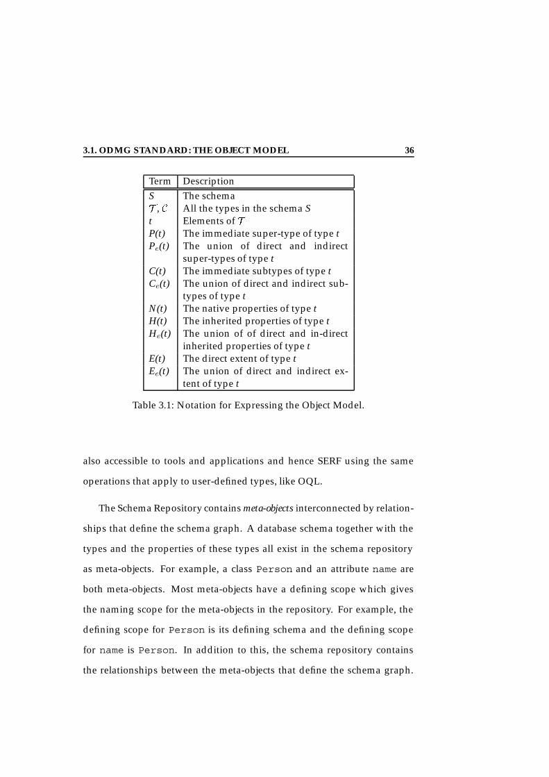
3.1. ODMG STANDARD: THE OBJECT MODEL 36
Term DescriptionS The schemaT , C All the types in the schema St Elements of TP(t) The immediate super-type of type tPe(t) The union of direct and indirect
super-types of type tC(t) The immediate subtypes of type tCe(t) The union of direct and indirect sub-
types of type tN(t) The native properties of type tH(t) The inherited properties of type tHe(t) The union of of direct and in-direct
inherited properties of type tE(t) The direct extent of type tEe(t) The union of direct and indirect ex-
tent of type t
Table 3.1: Notation for Expressing the Object Model.
also accessible to tools and applications and hence SERF using the same
operations that apply to user-defined types, like OQL.
The Schema Repository contains meta-objects interconnected by relation-
ships that define the schema graph. A database schema together with the
types and the properties of these types all exist in the schema repository
as meta-objects. For example, a class Person and an attribute name are
both meta-objects. Most meta-objects have a defining scope which gives
the naming scope for the meta-objects in the repository. For example, the
defining scope for Person is its defining schema and the defining scope
for name is Person. In addition to this, the schema repository contains
the relationships between the meta-objects that define the schema graph.

3.1. ODMG STANDARD: THE OBJECT MODEL 37
A class Person related to the class Address and the inheritance between
two classes are examples of such relationships. These relationships help
guarantee the referential integrity of the meta-object graph. Table 3.2 de-
fines accessor functions used in the later sections.
Function Return Type Return Descriptiont.localAttrlist Set Local properties of type tt.scope Schema Scope of type tt.metaClassName String Name of type tp.attrName String Name of property pp.attrType String Domain type of property pp.scope Class Scope of property p
Table 3.2: Commonly used Accessor Functions in the SERF Templates.
3.1.2 ODMG’s Object Query Language - OQL
As part of its standard, ODMG has defined an object query language OQL
that supports the ODMG data model. OQL is similar in format and fea-
tures to SQL 92 but has extensions for some object-oriented notions such
as complex objects, object identity, path expressions, polymorphism, oper-
ation invocation and late binding. In this section we describe a subset of
the language that is used for the examples in the paper. For a complete
description of OQL the reader is referred to [Cea97].
Selection. As a stand-alone query language, OQL supports the query-
ing over any kind of object (i.e., individual object instances, collections and
even the meta-data in the schema repository) starting from their names
which act as entry points to the database. OQL supports querying with

3.1. ODMG STANDARD: THE OBJECT MODEL 38
and without object identifiers. For example, if the schema defines the types
Person and Employee with extents Persons and Employees then it is
possible to query Persons as follows:
select distinct x.age
from Persons x
where x.name = "Pat"
This selects the set of ages of all persons named Pat, returning a literal
of type set<integer>.
select x
from Persons x
where x.name = "Pat"
This selects all persons with the name Pat, returning a literal of type
set<Person> where each Person object in the resultant set has the same
object identifier as that in the database.
Creation. OQL supports the creation of objects both with and without
identity. For example, Person(name: "Pat",
birthdate: "3/28/95", salary:10000) creates an instance of the
type Person using the Person type constructor. This constructs a new
Person object with a new object identifier. Similarly, struct (name:
"Pat" , birthdate: "3/28/95" , salary: 10000 ) yields a
structure with three fields but no object identity.

3.2. EVOLVING THE ODMG OBJECT MODEL 39
Path Expressions. The ODMG object model as mentioned in Section 3.1
supports the naming of objects and also the reachability of other objects
through this named object (i.e., persistence by reachability). From OQL,
one therefore needs a way to navigate from a named object and reach the
desired data. For example, the query
p.spouse.address.city.name starts from a Person, gets her spouse (a
Person again) goes inside the complex attribute of type Address to get
the City object whose name is then accessed.
Method Invocation. OQL can call a method with or without parameters
anywhere the result type of the method matches the expected type in the
query. For example,
select p.oldest-child.address
from Persons p
where p.lives-in(‘‘Paris’’)
In this statement we retrieve the address of the oldest-child of
all Persons who live in Paris. Here oldest-child is a method that
takes no parameters and returns an object of type Person. The method
lives-in is applied to the Person object and takes one parameter of the
type String and returns true if the specific person lives in the target city.
3.2 Evolving the ODMG Object Model
Some support for schema evolution is provided by most OODBs [BKKK87,
Tec94, BMO+89, Inc93, Obj93]. However, the ODMG 2.0 standard does not
3.2. EVOLVING THE ODMG OBJECT MODEL 40
yet address the issue of schema evolution. In this section we therefore de-
scribe a taxonomy of primitives to provide support for dynamic schema
evolution of the ODMG object model based on a representative set found
in other OODBs [BKKK87, Tec94, BMO+89, Inc93, Obj93]. We first present
the invariants for preserving the ODMG object model and then the schema
evolution primitives that preserve these invariants and hence the object
model. The primitives presented here are minimal in that they cannot be
decomposed into any other evolution primitives and essential in that they
are all required for the evolution of the given object model. They can how-
ever be composed together with other evolution primitives to form more
complex transformations, as we show in later sections.
3.2.1 Invariants for the ODMG Object Model
A schema update can cause structural inconsistencies. An important prop-
erty imposed on schema operations is thus that their application always
results in a consistent new schema [BKKK87]. The structural consistency of
a schema is defined by a set of schema invariants of the given object model
[Bre96]. In this section, we present the invariants for the ODMG object
model adapted from the axiomatic model proposed by Peters and Ozsu
[PO95].
Table 3.3 shows the notation we use for describing the axiomatic model.
The in-paths and the out-paths are a set of pairs of <type, name>, i.e., a
pair <c1, r1> where c1 is the name of the class referring to t (or the class
being referred to by t) and r1 is the name of the reference attribute. The
in-degree and the out-degree of a type is given by the count of all the types

3.2. EVOLVING THE ODMG OBJECT MODEL 41
Term Descriptiontypes(C) All the types in the systemS The schemaT All the types in the schema SC All the types in the schema St Elements of TP(t), super(t) The immediate super-type of type tPe(t),super(t) The union of direct and indirect super-types of type
tC(t), sub(t) The immediate subtypes of type tCe(t), sub(t) The union of direct and indirect subtypes of type tN(t) The native properties of type tH(t) The inherited properties of type tHe(t) The union of of direct and in-direct inherited prop-
erties of type tE(t) The direct extent of type tEe(t) The union of direct and indirect extent of type tin-paths(t) The set of all paths referring to type tin-degree(t) The count of all paths referring to type tout-paths(t) The set of all paths going out of type tH-out-paths(t) The set of all inherited out-paths of type tout-degree(t) The count of all paths going out of type tself-degree(t) The count of all self paths of type tH-out-degree (t) The count of all H-out-paths(t) that are not self-
referentialT-IN(t) The total in-degree: in-degree(t) + self-degree(t)T-OUT(t) The total out-degree: out-degree(t) + self-degree(t) + H-
out-degree(t)R The set of all relations in the system
Table 3.3: Notation for Axiomatization of Schema Changes
other than itself referring to the type and vice versa. The self-degree is the
count of self-references for a type. Thus the total in-degree, T-IN, of a type
is given by the sum of the in-degree and the self-degree. Similarly, the total
out-degree, T-OUT, is the sum of the out-degree, the self-degree and the
3.2. EVOLVING THE ODMG OBJECT MODEL 42
inherited out-degree.
The following invariants hold:
1. Rootedness. There is a single type t 2 T that is the super-type of all
types in T . The type t is called the root of the type lattice (T ).
2. Closure. Every type in T , excluding root, has a super-type in T , giv-
ing closure to T .
3. Pointedness. There are one or more types ? 2 T such that ? has no
subtypes in T . ? is termed a leaf of the type lattice.
4. Singularity. Every type t 2 T , excluding the root, has exactly one
direct super-type ts in T , i.e., j P(t) j = 1.
5. Distinction. Every type t 2 T has a distinct name, i.e., 8 t1, t2, if
t1.name = t2.name, then t1 = t2. Every property p for a type t has
a distinct name; the scope of name distinction for a property is the
union of the inherited and native properties for type t.
6. Degree. The ratio of total in-degree, T-IN of the schema , to the total
out-degree, T-OUT of the schema is an invariant.
3.2.2 Taxonomy of Schema Evolution Primitives
In this section we present the taxonomy of schema evolution primitives
that we have designed for the ODMG object model such that they preserve
the invariants introduced in Section 3.2.1 (Table 3.4). Our goal is to achieve
a set of schema evolution primitives that is:

3.2. EVOLVING THE ODMG OBJECT MODEL 43
• Complete, i.e., our primitive set subsumes every possible type of struc-
tural schema change within the ODMG model.
• Minimal, i.e., none of the primitives can be achieved by a combination
of two or more primitives.
• Consistent, i.e., each primitive is guaranteed to generate a valid sch-
ema as output when applied to a valid input schema. If the input
schema is invalid, the operation is ignored and the schema is un-
changed.
Completeness of Evolution Primitives. The taxonomy that we present
here captures all changes needed to manipulate the ODMG type lattice as
given in Section 3.1. We now outline a proof that shows that this set of
changes indeed subsumes every possible type of schema change (complete-
ness criteria). The proof we sketch has its basis on the completeness proof
given by Banerjee et al. for the evolution taxonomy of Orion [BKKK87].
In order to show completeness of these operations we prove that every
legal type lattice as defined by the invariants is achievable by combining
the operations given in Table 3.4.
Lemma 1 For any given type lattice T, there is a finite sequence of op2, op7 and
op9 that can reduce the type lattice T to a type lattice T’ consisting of only one
single type, a root type.
Proof: Assume that the type lattice has no relationships. It is apparrent
if we repeatedly apply the operation op2 which removes a leaf type t, we

3.2. EVOLVING THE ODMG OBJECT MODEL 44
Num Evolution Primitive Description Error Conditionop1 add-class(c, C) Add new class c to C
in the schema SClass c already ex-ists in S
op2 delete-class(c) Delete class c from Cin the schema S
c has sub-classes
op3 add-ISA-edge(cx, cy) Add an inheritanceedge from class cx tocy
there exists an edgefrom some class cz
to cy
op4 add-attribute(cx, ax, t, d) Add attribute ax oftype t and defaultvalue d to class cx
and to all its sub-classes
ax already exists incx
op5 delete-attribute(cx, ax) Delete the attributeax from the class cx
and removes it fromall its subclasses
ax does not exist inclass cx
op6 add-reference-attribute(cx,rx, cy , d)
Add unary relation-ship from class cx
to class cy named rx
with default value d
rx already exists incx
op7 delete-reference-attribute(cx, rx)
Delete unary rela-tionship in class cx
named rx
rx does not exist incx
op8 form-relationship(cx, rx,cy, ry)
Promote the speci-fied two unary rela-tionships to a binaryrelationship
rx and ry do not ex-ist in classes cx andcy respectively
op9 drop-relationship(cx, rx,cy, ry)
Demote the speci-fied binary relation-ship to two unaryrelationships
rx and ry are notpart of the same bi-directional relation-ship
Table 3.4: Taxonomy of Basic Schema Evolution Primitives. The full alge-braic expressions for these are given in Table 3.7.
can after a finite number of applications reduce any given type lattice T to
a new type lattice T’ which only has one type, i.e., its root.
Now assume that we have relationships in the type lattice. A repeated

3.2. EVOLVING THE ODMG OBJECT MODEL 45
application of op9 and op7will after a finite number reduce the type lattice
T to a type lattice T’ with no relationships. The reduction of T’ to a type
lattice T’’ with a single root follows from the discussion above.
Lemma 2 There is a finite sequence of operations op1, op3, op4, op6, op8 that generates any desired type lattice T from an empty type lattice T’.
Proof: Consider that we have two type lattices T and T’. Let T be a type
lattice with a finite number of types, edges and one root, and T’ be a type
lattice with only a root node, i.e., a schema with just a root. The following
procedure can, via the finite sequence of operations listed above, transform
the type lattice T’ to become identical to the type lattice T. Traverse type
lattice T in a breadth-first order and perform the following for each type t
visited:
• For every type t in T, add a corresponding type t’ to type lattice T’
(and hence also T ’ using the operation op1.
• Add all local properties p of type t to the new type t’ in T’ using
the operation op5.
• For the incoming edge into the type t, add a corresponding incoming
edge to the node t’ in T using the operation op3.
Once all the types are built, build the relationships between the types,
if any, using the operation op6 and op8.
The resultant type lattice T’ is equivalent to the initial type lattice T as
they have the same set of types and the same type lattice. 2

3.2. EVOLVING THE ODMG OBJECT MODEL 46
Theorem 1 Given two arbitrary type lattices T and T’, there is a finite sequence
F of operations from op1, op3, op4, op5, op6, op7, op8, op9 , such that
when F is applied to the type lattice T it produces the type lattice T’.
Proof: We can prove this by first reducing the type lattice T to an in-
termediate type lattice T1 using Lemma 1. The type lattice T1 can then be
converted to the type lattice T’ using Lemma 2. 2
The set of operations op1, op3, op4, op5, op6, op7, op8, op9 is a
subset of the taxonomy of operations given in Table 3.4. Hence the com-
pleteness of this set of operations follows from Theorem 1.
Minimality of Evolution Primitives. Following the Orion schema evo-
lution taxonomy [BKKK87], we have kept the schema changes add-class,
add-attribute, delete-attribute and add-ISA-edge as primitives in our basic set.
We have excluded the schema change change-name-of-attribute and rename-
class as they can be achieved by the composition of two other primitives.
For example, change-name-of-attribute can be accomplished by add-attribute
followed by copying values from the old attribute to the new one followed
by delete-attribute of the old attribute. A library of these basic transforma-
tions which are not minimal yet may be very common and hence useful
can be provided by SERF2. We have replaced the schema change drop-class
from the Orion taxonomy with the delete-class operation which removes a
leaf class. This is due to the fact that the drop-class can have many different
semantics, each of which can be achieved by combining other primitives
2In the later sections we show how SERF can be used to achieve transformations bycombining the primitives given in Table 3.4.

3.2. EVOLVING THE ODMG OBJECT MODEL 47
given in Table 3.4. We also do not consider the operation delete-ISA-edge as
part of the primitive set. The semantics of this operation can be achieved
by a combination of the delete-class and add-ISA-edge operations.
A proof for the minimality of our operation set follows from Theorem 1.
add-class Primitive delete-class Primitivefunction add-class (type : t, types: T )
pre-condition:t /2 T
if T = ;, then root = tT T
St
C(root) C(root)St
P(t) P(t)St
C(t) ;N(t) ;H(t) N(root)E(t) ;
function delete-class (type : t, types: T )
pre-condition:t 2 T andC(t) = ; andt 6= root
T T tfor all s 2 Pe(t):
C(s) C(s) tEe(s) Ee(s) E(t)
delete N(t)delete H(t)delete E(t)
Table 3.5: The Schema Evolution Primitives.
Consistency of Evolution Primitives. Tables 3.5 through 3.7 define the
evolution primitives given in Table 3.4. No object transformations are indi-
cated in these functions. Each of these primitives preserves the invariants
listed in Section 3.2.1 and hence always produces a consistent schema when
given a consistent schema. For example, the
delete-class primitive deletes the specified type from the set of types
T . We assume here that the schema is consistent before the operation is
invoked. The delete-class preserves:
• Invariant 1 - by disallowing the deletion of the root type (precondi-

3.2. EVOLVING THE ODMG OBJECT MODEL 48
add-ISA-edge Primitivefunction add-ISA-edge (type : x, type: y)
pre-condition:P(y) = root andx 6= root
P(y) P(y) rootC(root) C(root) y
Ce(x) Ce(x)SCe(y)
P(y) xfor all t 2 Ce(y):
Pe(t) Pe(t)SPe(x)
H(y) H(y)SN(x)
He(y) H(y)SHe(x)
for all t 2 Ce(y):He(t) He(t)
SHe(y)
for all s 2 Pe(y):Ee(s) Ee(s)
SEe(y)
Table 3.6: The Schema Evolution Primitives.
add-attribute Primitive delete-attribute Primitivefunction add-attribute (type : t, at-tribute: a)
pre-condition:a /2 N(t) anda /2 H(t) andfor all c 2 Ce(t):
a /2 N(c)SH(c)
N(t) N(t)Sa
for all c 2 Ce(t):H(c) H(c)
Sa
function delete-attribute (type : t, at-tribute: a)
pre-condition:a 2 N(t)
N(t) N(t) afor all c 2 Ce(t):
H(c) H(c) a
Table 3.7: The Schema Evolution Primitives.
tion 3), we guarantee that this root will stay unique in the schema.
• Invariant 2 - by allowing a type to be deleted only if it is a leaf type,

3.2. EVOLVING THE ODMG OBJECT MODEL 49
add-reference-attributePrimitive
delete-refernce-attributePrimitive
function add-reference-attribute ( Cs, r,Cd, default) precondition:
Cs, Cd 2 C andr /2 N(Cs)N(Cs) N(Cs)
Sr
in-path(Cd) in-path(Cd)S<Cs,r>
out-path(Cs) out-path(Cs)S<Cd,r>
8 Cx 2 sub(Cs)out-path(Cx) out-path(Cx)S
<Cd,r>
function delete-reference-attribute ( Cs,r)
precondition:Cs 2 C andr 2 N(Cs) anddomain(r) 2 C
N(Cs) N(Cs) - rin-path(domain(r))
in-path(domain(r))- <Cs,r>
out-path(Cs) out-path(Cs)- <domain(r),r>
8 Cx 2 sub(Cs)out-path(Cx) out-path(Cx)
- <domain(r),r>
form-relationship Primitive drop-relationship Primitivefunction form-relationship ( Cs, rs, Cd,rd )
precondition:Cs, Cd 2 C andrs 2 N(Cs) andrd 2 N(Cd) and<Cs, rs > 2 in-path(Cd) and<Cd, rd > 2 in-path(Cs)
α1(rd) = rs and α(rs) = rd
function drop-relationship ( Cs, rs, Cd,rd )
precondition:Cs, Cd 2 C andrs 2 N(Cs) andrd 2 N(Cd) and<Cs, rs > 2 in-path(Cd) and<Cd, rd > 2 in-path(Cs) andα1(rd) = rs and α(rs) = rd
:(α1(rd) = rs and α(rs) = rd )
Table 3.8: The Schema Evolution Primitives. Here α represents the seman-tics of a binary relationship [CRH01].
thereby ensuring that there are no subtypes whose supertype is not
in T .
• Invariant 3 - esnures that t is a leaf node when deleted.
3.3. SUMMARY 50
• Invariant 4 - not affected.
• Invariant 5 - not affected.
Similarly, by inspection of all the primitives given in Table 3.5 through
to 3.7, we can show that they are sound and generate a consistent schema,
preserving all invariants.
3.3 Summary
In this chapter we have presented the essential background that is needed
for the remainder of this part on SERF. In particular we have described the
ODMG object model and presented a detailed taxonomy for evolving an
ODMG-compliant schema.
51
Chapter 4
The SERF Framework
In this chapter we present the fundamental principles of our SERF trans-
formation framework [CJR98c, CJR98a, CRed, RCL+99]1. In particular, we
demonstrate how our framework succeeds in giving users the flexibility to
define the semantics of their choice, the extensibility of defining new com-
plex transformations, and the re-usability of these transformations through
the notion of templates.
4.1 Features of the Framework
The SERF framework addresses the limitations of current OODB technol-
ogy that restrict schema evolution to a predefined set of operations with fixed
semantics. In particular, our goal is to support arbitrary user-customized and
possibly complex schema evolution operations. Similar to [Bre96], our first
step in this direction is to allow users to build new schema transformations
1This work was done in collaboration with Jin Jing, a Masters student at WPI [Jin98].
4.1. FEATURES OF THE FRAMEWORK 52
with customized semantics using a fixed set of schema evolution primitives
provided by the underlying OODB system (see Section 3.2.2.).
While our work is based on describing complex schema transforma-
tions using a fixed set of basic schema evolution primitives, a pure se-
quence of these schema evolution primitives is not always powerful enough
to express many desired transformations. For example, Figure 4.1 shows a
schema transformation that creates a new class MergePapers based on
the two input classes Author and Paper. The class MergePapers is con-
structed by collecting some of the attributes that exist Author and Paper.
For example, we might only want to add the attribute AuthorName if it
exists in both the classes Author and Paper. And in this case, we want to
add it only once. There is no pure sequence of schema evolution operations
that could characterize this logic of attribute selection for MergePapers.
Thus, we recognize the need to have some language as “glue logic”. More-
over, such a language is also needed to achieve value-based transforma-
tions of objects across types. For example, if we are adding AuthorName
from Author we might also want to take the value of AuthorName from
the instances of Author. In current OODB systems, to achieve these types
of transformations users have to resort to writing ad hoc code using a pro-
gramming language. This has the drawback of being both programming
language and system dependent, and hence not portable. Moreover, it is
much harder task to reason and prove the consistency of a transformation
written in a programming language.
We therefore advocate the use of a declarative query language, such as
OQL, as a transformation language. The query language must have an in-

4.1. FEATURES OF THE FRAMEWORK 53
Figure 4.1: An Example Schema Graph for a MERGE Transformation.
terface for invoking the schema evolution primitives, as those provide the
basic mechanism for changing the type structure. The query language must
also have the expressive power for realizing any arbitrary object manipu-
lations to transform objects from one object type to another. In Section 5.1,
we will show that this approach also guarantees consistency for all schema
transformations.
In our framework, these arbitrarily complex transformations can be en-
capsulated and generalized by assigning a name and a set of parameters to
them. From here on these are called transformation templates or templates for
short. By parameterizing the variables involved in a transformation, such
as the input and output classes and their properties, a transformation be-
comes a generalized reusable module applicable to any application schema.
By assigning a name to such a template, it can also now be re-used from
within other transformations. This leads us to the idea of collecting tem-
plates in a template library and thus guaranteeing the availability of tem-
plates to any user at any time, just as the fixed set of schema evolution
operations are available to users in any regular schema evolution system.
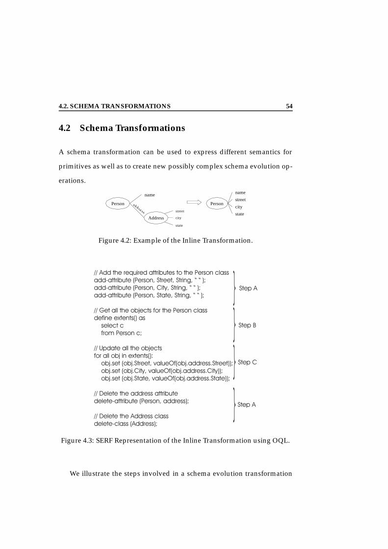
4.2. SCHEMA TRANSFORMATIONS 54
4.2 Schema Transformations
A schema transformation can be used to express different semantics for
primitives as well as to create new possibly complex schema evolution op-
erations.
Person
name
Address
address street
city
state
Person
name
street
city
state
Figure 4.2: Example of the Inline Transformation.
Figure 4.3: SERF Representation of the Inline Transformation using OQL.
We illustrate the steps involved in a schema evolution transformation
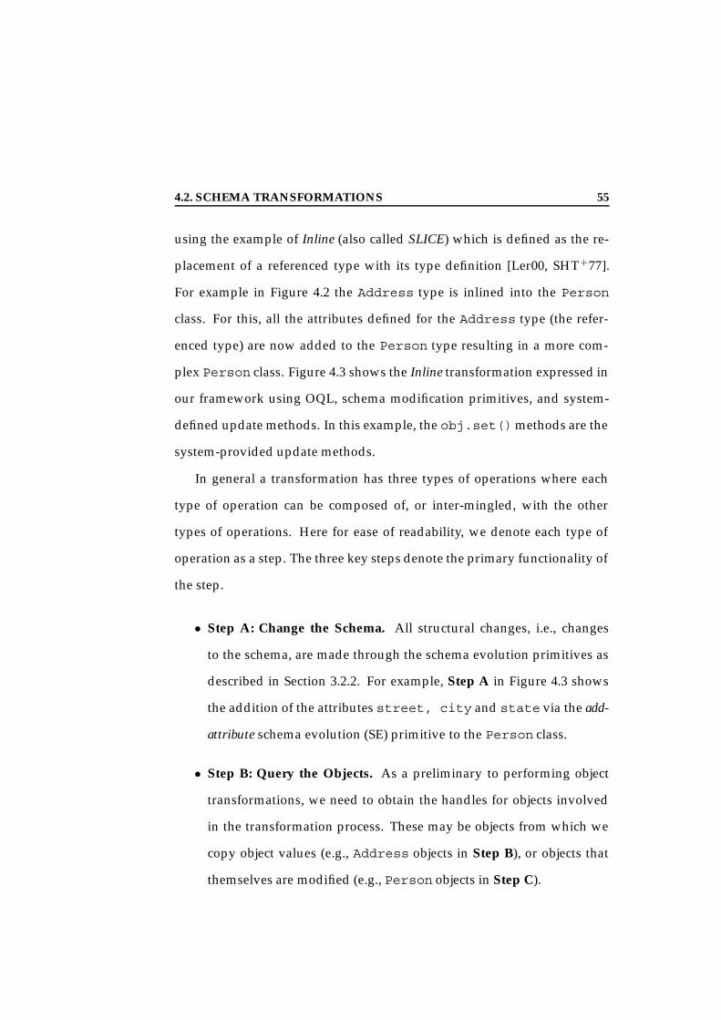
4.2. SCHEMA TRANSFORMATIONS 55
using the example of Inline (also called SLICE) which is defined as the re-
placement of a referenced type with its type definition [Ler00, SHT+77].
For example in Figure 4.2 the Address type is inlined into the Person
class. For this, all the attributes defined for the Address type (the refer-
enced type) are now added to the Person type resulting in a more com-
plex Person class. Figure 4.3 shows the Inline transformation expressed in
our framework using OQL, schema modification primitives, and system-
defined update methods. In this example, the obj.set()methods are the
system-provided update methods.
In general a transformation has three types of operations where each
type of operation can be composed of, or inter-mingled, with the other
types of operations. Here for ease of readability, we denote each type of
operation as a step. The three key steps denote the primary functionality of
the step.
• Step A: Change the Schema. All structural changes, i.e., changes
to the schema, are made through the schema evolution primitives as
described in Section 3.2.2. For example, Step A in Figure 4.3 shows
the addition of the attributes street, city and state via the add-
attribute schema evolution (SE) primitive to the Person class.
• Step B: Query the Objects. As a preliminary to performing object
transformations, we need to obtain the handles for objects involved
in the transformation process. These may be objects from which we
copy object values (e.g., Address objects in Step B), or objects that
themselves are modified (e.g., Person objects in Step C).

4.3. TRANSFORMATION TEMPLATES 56
• Step C: Change the Objects. The next step to any schema transforma-
tion is the transformation of the objects to conform to the new schema.
Through Step B, we already have a handle to the affected object set.
Step C in Figure 4.3 shows how a query language, such as OQL, and
system-defined update methods, such as obj.set(...), can be used to
perform object transformations.
In general, a transformation in SERF uses a query language to query
over the application objects, as in Step B. The transformation also uses
the query language to invoke the schema evolution primitives (such as
add-attribute() in Step A) and update methods for updating the ob-
jects (such as obj.set() in Step C ).
In this example, we simply added attribute values to the existing ob-
jects. In some transformations, existing objects might need to be deleted or
new objects might be created. OQL allows for the creation of new objects
through a constructor-like statement. Deletion of objects has to be done by
a system-defined update method.
4.3 Transformation Templates
Figure 4.3 showed how a schema transformation that inlined the Address
class into the Person class using OQL, schema primitives, and update
methods. Embedding schema evolution operations in OQL allows the user
to achieve any desired transformation. This is a big step above the fixed set
of schema evolution primitives offered by previous approaches. However,
this can also be compared to the functionality of a custom program in a
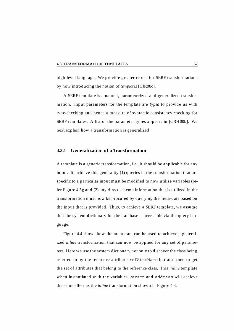
4.3. TRANSFORMATION TEMPLATES 57
high-level language. We provide greater re-use for SERF transformations
by now introducing the notion of templates [CJR98c].
A SERF template is a named, parameterized and generalized transfor-
mation. Input parameters for the template are typed to provide us with
type-checking and hence a measure of syntactic consistency checking for
SERF templates. A list of the parameter types appears in [CRH00b]. We
next explain how a transformation is generalized.
4.3.1 Generalization of a Transformation
A template is a generic transformation, i.e., it should be applicable for any
input. To achieve this generality (1) queries in the transformation that are
specific to a particular input must be modified to now utilize variables (re-
fer Figure 4.5); and (2) any direct schema information that is utilized in the
transformation must now be procured by querying the meta-data based on
the input that is provided. Thus, to achieve a SERF template, we assume
that the system dictionary for the database is accessible via the query lan-
guage.
Figure 4.4 shows how the meta-data can be used to achieve a general-
ized inline transformation that can now be applied for any set of parame-
ters. Here we use the system dictionary not only to discover the class being
referred to by the reference attribute refAttrName but also then to get
the set of attributes that belong to the reference class. This inline template
when instantiated with the variables Person and address will achieve
the same effect as the inline transformation shown in Figure 4.3.

4.3. TRANSFORMATION TEMPLATES 58
Figure 4.4: Generalized Inline Template based on the Inline Transforma-tion.
4.3.2 Template Library
While most databases today provide some support for schema evolution,
it is very specific to the underlying OODB. Thus, we propose the develop-
ment of a library of schema evolution templates that can be ported across
OODBs as long as the system requirements as set forth in [CJR98d] are met.
Thus SERF templates for a particular domain are collected in a Tem-
plate Library. Simple key-word search is available on all stored parameters
of the template such as the input and output parameters, the name, and
its description. Inheritance and other semantic relationships between tem-

4.3. TRANSFORMATION TEMPLATES 59
plates are defined to facilitate a multi-level organization of the template li-
brary. Such a template library will be an important resource in the schema
evolution community, much like other re-usable libraries in software engi-
neering.
4.3.3 SERF Template Language
A SERF template is thus a named sequence of OQL statements extended
with a name, parameters and variables that can be translated to pure OQL
statements during the process of instantiation. The BNF for a SERF template
is given in Figure 4.5. In the BNF restricted query denotes the OQL
query limited to invoking only object updates and the schema evolution
primitives.
4.3.4 SERF Template Instantiation and Processing
During the instantiation process, the SERF template specification is trans-
lated to pure OQL statements. Prior to the instantiation it is assumed that
a database on which the template is to be executed has already been se-
lected, and we are in the context of this database environment. A consis-
tency and bind check is performed both before and after the instantiation
of the template. Figure 4.6 shows the steps for the execution of a template.
When a template is created, the user can assign a name to it and also spec-
ify its parameters. A compile-time syntax check is performed for both the
OQL queries and the system function in the template. When the template
is instantiated, the caller provides bindings for the parameters. A second
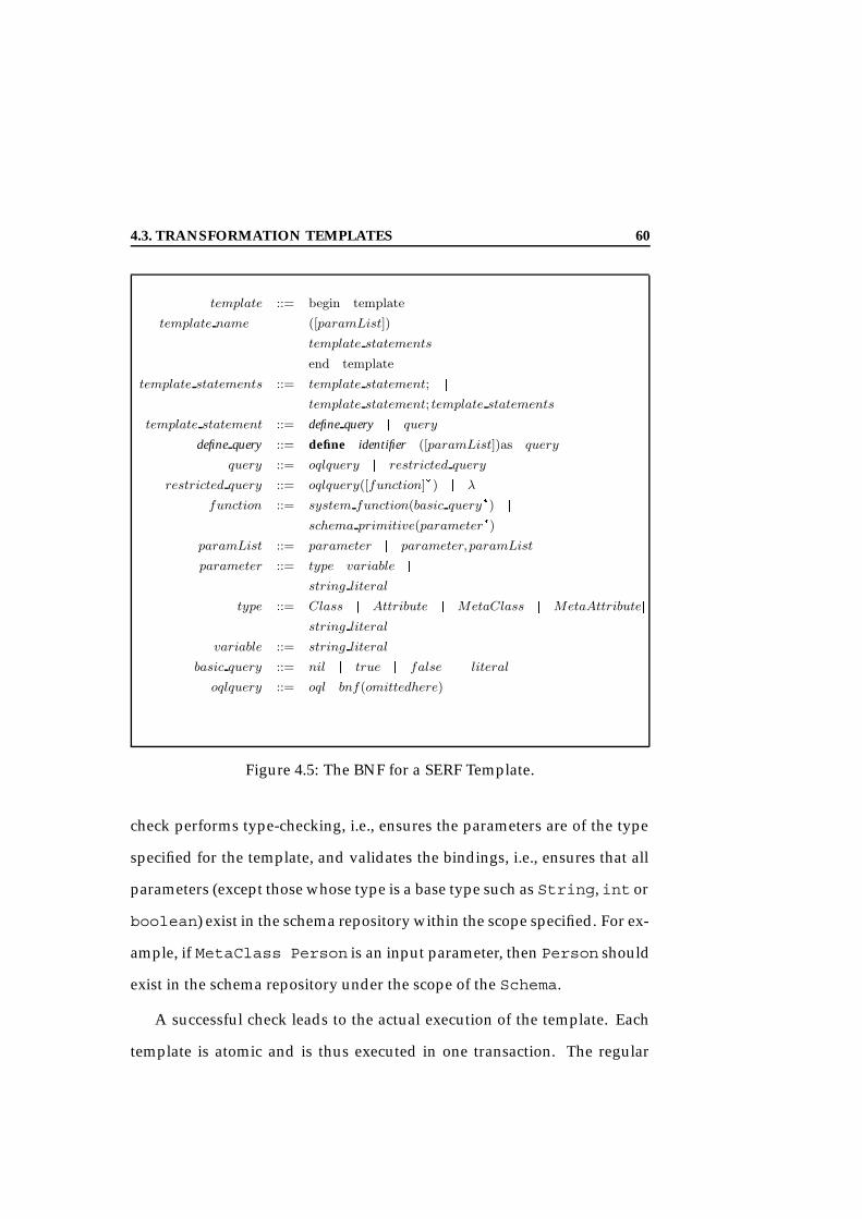
4.3. TRANSFORMATION TEMPLATES 60
template ::= begin template
template name ([paramList])
template statements
end template
template statements ::= template statement; j
template statement; template statements
template statement ::= define query j query
define query ::= define identifier ([paramList])as query
query ::= oqlquery j restricted query
restricted query ::= oqlquery([function]) j λ
function ::= system function(basic query) j
schema primitive(parameter)
paramList ::= parameter j parameter,paramList
parameter ::= type variable j
string literal
type ::= Class j Attribute j MetaClass j MetaAttributej
string literal
variable ::= string literal
basic query ::= nil j true j false j literal
oqlquery ::= oql bnf(omittedhere)
Figure 4.5: The BNF for a SERF Template.
check performs type-checking, i.e., ensures the parameters are of the type
specified for the template, and validates the bindings, i.e., ensures that all
parameters (except those whose type is a base type such as String, int or
boolean) exist in the schema repository within the scope specified. For ex-
ample, if MetaClass Person is an input parameter, then Person should
exist in the schema repository under the scope of the Schema.
A successful check leads to the actual execution of the template. Each
template is atomic and is thus executed in one transaction. The regular
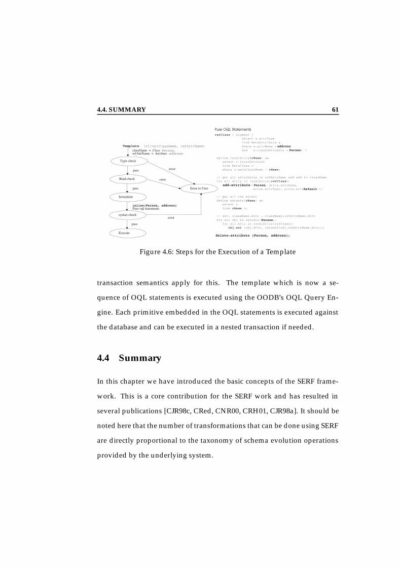
4.4. SUMMARY 61
Figure 4.6: Steps for the Execution of a Template
transaction semantics apply for this. The template which is now a se-
quence of OQL statements is executed using the OODB’s OQL Query En-
gine. Each primitive embedded in the OQL statements is executed against
the database and can be executed in a nested transaction if needed.
4.4 Summary
In this chapter we have introduced the basic concepts of the SERF frame-
work. This is a core contribution for the SERF work and has resulted in
several publications [CJR98c, CRed, CNR00, CRH01, CJR98a]. It should be
noted here that the number of transformations that can be done using SERF
are directly proportional to the taxonomy of schema evolution operations
provided by the underlying system.

4.4. SUMMARY 62
63
Chapter 5
Soundness and Consistency of
SERF Templates
In this chapter, we show how the SERF templates can assure the soundness
of the database after their execution as well as show how users can specify
their own constraints which must then be preserved by the execution of the
template [CRed, CRH00a, CRH01]1.
5.1 Soundness of Templates
An important property imposed on schema operations is that their exe-
cution on a consistent schema always results in a consistent new schema
[BKKK87] with consistency as defined by the invariants of the data model.
In Section 3.2.2 we have showed via an example and by complete defini-
1This work was done in collaboration with George T. Heineman, Associate Professor atWPI.
5.1. SOUNDNESS OF TEMPLATES 64
tion of the primitives, that the schema change primitives for the ODMG
object model as defined in Section 3.1 indeed preserve the consistency of
a schema. Thus, an individual schema evolution primitive (Section 3.2.2)
when applied on a consistent schema will always generate a consistent
schema. In this section, we now extend this notion of soundness to SERF
templates.
We utilize the type lattice and the set of nine operations on the type
lattice, represented by OP, presented in Section 3.2.2 to show the soundness
of SERF templates. Here the type lattice T represents a schema conforming
to the invariants and the operations correspond to the evolution primitives
in Table 3.4. Towards showing soundness of SERF templates, we first state
the following lemma.
Lemma 3 A sequence Pn of operations ho1, . . . oi . . . oni, where oi 2 OP
(Table 3.4), and 1 i n when applied to a consistent type lattice T generates a
consistent type lattice T’.
Proof: By Induction on number of operations opi in a sequence:
Basis - Let P be a sequence of one operation, i.e., n = 1.
P1 = h o1 i, where o1 2 OP.
We have shown in Section 3.2.2 that any operation o 2 OP when applied
to a consistent type lattice T generates a consistent type lattice T’ or leaves
the original lattice unchanged. This is denoted as T P1=) T’.
Assumption: For a sequence Pk of k-operations, with Pk = ho1 . . . oi . . . oki,
where oi 2 OP, i = 1 . . . k and T is a consistent type lattice, then TPk=) T’
generates a consistent type lattice T’.

5.1. SOUNDNESS OF TEMPLATES 65
Induction: Now let n = k+1 such that Pk+1 is a sequence of k + 1 opera-
tions and Pk+1 = h o1 . . . oi . . . ok, ok+1 i, where oi 2 OP, i = 1 . . . k+1.
That is, Pk+1 = Pk ok+1. We need to prove the following:
TPk+1=) T’.
To achieve this we can apply the first k operations of Pk+1. Let us denote
them by Pk. We know from our assumption that Pk, when applied to a
consistent type lattice T, produces another consistent type lattice Tk. We
can then apply the k+1th operation to Tk by induction basis. Thus we have,
TPk=) Tk
opk+1=) T’,
Thus we have, TPk+1=) T’ and the generated T’ is a consistent type lattice.2
Using the above result, we now state the theorem for the soundness of
the SERF Templates.
Theorem 2 A SERF template when applied to a consistent schema conforming to
the specified object model (Section 3.1) will always result in a consistent schema as
defined by the invariants in Section 3.2.1.
Proof: A SERF template has three main components: (1) schema evolution
primitives; (2) queries on the application or meta-data; and (3) object up-
dates expressed in OQL. We exclude (2) and (3) on the basis that these do
not in any way alter the structure of the schema and hence do not violate
the invariants of the object model as presented in Section 3.2.1. In a SERF
template any composition of schema evolution primitives results in the se-
quential execution of the primitives in that composition. The soundness of
the SERF templates follows from Lemma 3. 2
5.2. CONTRACTS 66
Here we do not guarantee the consistency of the data after the applica-
tion of a SERF template, but only that of the schema. Data updates are
made during the execution of a schema evolution primitive and by the
queries in the SERF template. Guaranteeing the consistency of these data
updates is outside the scope of discussion here.
5.2 Contracts
Conventionally, schema evolution primitives contain hard-coded constrai-
nts that parallel the invariants of the object model. These constraints must
be satisfied in order to guarantee the consistency of the system. While
a SERF template also preserves these invariants as shown in Section 5.1,
the SERF template may itself have additional constraints that now specify
user-level constraints that are to be imposed on the SERF template. We in-
troduce the notion of contracts, a declarative mechanism for expressing the
constraints for a template and now define a ROVER Wrapper as a template
with contracts. This approach also has the advantage that a change in the
object model results in a change in the invariants of the model and conse-
quently in the re-engineering of the schema evolution primitives. Contracts
can now also be used to decouple the invariant constraints from the actual
implementation of the schema evolution primitives. Changes to the invari-
ants of the object model now merely result in the update of the declarative
contracts associated with the evolution operations rather than the update
of the actual system code. Below we briefly introduce contracts and show
how the decoupling of constraints can be achieved.

5.2. CONTRACTS 67
Contracts provide a declarative description of the behavior of a tem-
plate (or primitive) as well as a mechanism for expressing the constraints
that must be satisfied prior to the execution of the actual evolution primi-
tive. Contracts are divided into two categories preconditions and postcon-
ditions.
The constraints, termed preconditions, are placed prior to any body of
template code (OQL statements including system-defined schema evolu-
tion primitive). The preconditions are separated from the actual OQL state-
ments by means of the keyword requires. Postconditions, a set of contracts
that appear after the body of the actual schema evolution operation at the
end of the SERF template, specify the behavior of the primitives. These
postconditions are preceded by the keyword ensures and describe the ex-
act changes that are made to the schema by the evolution operator and
hence its behavior.
Example: As an example consider the addition of relationship constructs
to the object model of an OODB system. An upgrade to the schema evolu-
tion facility in this case requires new schema evolution primitives to han-
dle the creation, modification, and deletion of uni-directional and/or bi-
directional relationships. This upgrade cannot be circumvented and hence
new schema evolution primitives must be added to the system. However,
an update of all existing schema evolution operations to conform to the
new set of invariants is also required. For example, to delete a class prior to
the existence of relationships, the constraint that a class needed to be a leaf
class was necessary to ensure that the resulting schema and database was

5.2. CONTRACTS 68
consistent, i.e., delete-class preserved the database consistency. With
the addition of relationships, this constraint alone is not sufficient. We now
also need to ensure that the to-be-deleted Cs class is not referred to by
another class. Moreover, no objects in the database must refer to the objects
of the Cs class. So while the conditions that need to be enforced prior to
the execution the schema evolution operation have to be upgraded, the ac-
tual actions of the operations do not change. Hence the evolution primitive
delete-class itself does not change.
Figure 5.1 shows the constraints after the addition of a relationship for
the delete-class primitive as preconditions2. Thus, in this model it is
easy to extend or modify the constraints without re-writing the code for the
evolution primitive. Figure 5.2 shows the constraints that must be satisfied
after the execution of the template code.
delete-class ( Cs )
requires:Cs 2 T ^
C(Cs) = 0 ^in-degree(Cs) = 0 ^8 oi 2 extent(Cs)
obj-in-degree(oi) = 0
template body here
Figure 5.1: Preconditions forDelete-Class Primitive in Con-tractual Form.
delete-class ( Cs ) template body here
ensures:Cs /2 C ^8 <Cx, rx> 2 out-paths(Cs)
(<Cs> /2 in-paths(Cx))^
8 Cx 2 Pe(Cs)(Cs /2 sub(Cx) )
Figure 5.2: Postconditions for theDelete-Class Primitive Template.We assume here that the meta-dictionary information such asPe(Cx) are available until the tem-plate is done executing.
2The notation used here is a set-theoretic version of the contract language.
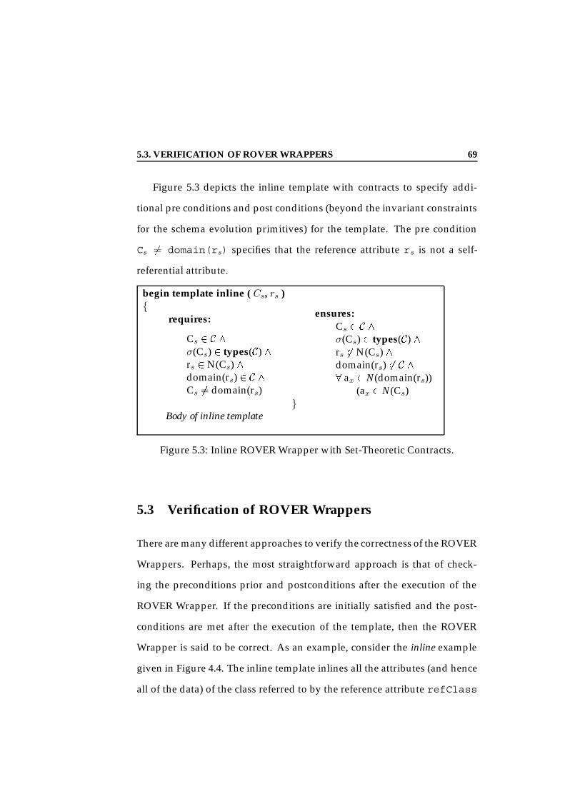
5.3. VERIFICATION OF ROVER WRAPPERS 69
Figure 5.3 depicts the inline template with contracts to specify addi-
tional pre conditions and post conditions (beyond the invariant constraints
for the schema evolution primitives) for the template. The pre condition
Cs 6= domain(rs) specifies that the reference attribute rs is not a self-
referential attribute.
begin template inline ( Cs, rs )
requires:
Cs 2 C ^
σ(Cs) 2 types(C) ^rs 2N(Cs) ^domain(rs) 2 C ^Cs 6= domain(rs)
Body of inline template
ensures:Cs 2 C ^
σ(Cs) 2 types(C) ^rs 62N(Cs) ^domain(rs) 62 C ^8 ax 2 N(domain(rs))
(ax 2 N(Cs)
Figure 5.3: Inline ROVER Wrapper with Set-Theoretic Contracts.
5.3 Verification of ROVER Wrappers
There are many different approaches to verify the correctness of the ROVER
Wrappers. Perhaps, the most straightforward approach is that of check-
ing the preconditions prior and postconditions after the execution of the
ROVER Wrapper. If the preconditions are initially satisfied and the post-
conditions are met after the execution of the template, then the ROVER
Wrapper is said to be correct. As an example, consider the inline example
given in Figure 4.4. The inline template inlines all the attributes (and hence
all of the data) of the class referred to by the reference attribute refClass

5.3. VERIFICATION OF ROVER WRAPPERS 70
into the class className. Once all attributes and data have been moved
over to className, the refClass is deleted. Now consider the scenario
that the reference attribute is a self-referencing attribute3. In such a case
after the execution of the delete-class primitive, the class refClass
= className is deleted which is clearly not the desired result as indi-
cated by the postconditions that require that classNamemust still exist on
completion of ROVER Wrapper execution. All changes made by the inline
template must be rolled back in such a scenario.
Thus while this approach verifies the correctness of the ROVER Wrap-
per, its fall-back for an erroneous change is a transaction roll-back which in
this case would be a rather expensive operation and hence not desirable.
An alternative to this is to use theorem proving to verify the correctness of
the ROVER Wrappers prior to their execution. A theorem prover based on
facts postulates the different states of the system for every statement that
is executed. Consider that the system is in state S0 of the system in which
all preconditions given in Figure 5.3 for the inline wrapper are met. The
theorem prover can now calculate the new state S1 which results from the
addition of an attribute. Let state Sn represent the state of the system af-
ter all attributes have been added. In state Sn, a delete-class primitive
would take the system to its final state Sf . If the state Sf does not meet the
desired postconditions as stated in the wrapper, then the wrapper is not
allowed to execute. In the following sections, we detail the basic require-
ments for a theorem prover and show via an example (inline template) how
the postconditions of the wrapper can be checked prior to execution.
3Inline assumes only one level of inlining, so recursion is not an issue here.
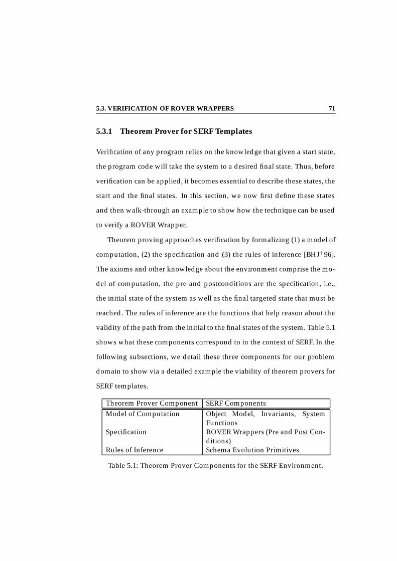
5.3. VERIFICATION OF ROVER WRAPPERS 71
5.3.1 Theorem Prover for SERF Templates
Verification of any program relies on the knowledge that given a start state,
the program code will take the system to a desired final state. Thus, before
verification can be applied, it becomes essential to describe these states, the
start and the final states. In this section, we now first define these states
and then walk-through an example to show how the technique can be used
to verify a ROVER Wrapper.
Theorem proving approaches verification by formalizing (1) a model of
computation, (2) the specification and (3) the rules of inference [BHJ+96].
The axioms and other knowledge about the environment comprise the mo-
del of computation, the pre and postconditions are the specification, i.e.,
the initial state of the system as well as the final targeted state that must be
reached. The rules of inference are the functions that help reason about the
validity of the path from the initial to the final states of the system. Table 5.1
shows what these components correspond to in the context of SERF. In the
following subsections, we detail these three components for our problem
domain to show via a detailed example the viability of theorem provers for
SERF templates.
Theorem Prover Component SERF ComponentsModel of Computation Object Model, Invariants, System
FunctionsSpecification ROVER Wrappers (Pre and Post Con-
ditions)Rules of Inference Schema Evolution Primitives
Table 5.1: Theorem Prover Components for the SERF Environment.

5.3. VERIFICATION OF ROVER WRAPPERS 72
Model of Computation for ROVER Wrappers. The model of computa-
tion formally describes the environment in which the theorem prover is
being applied. The SERF framework is based on the ODMG object model
(Section 3) [Cea97]. Hence, the theorem prover must be provided with a
formal definition of the ODMG object model, its invariants and the func-
tionality of each of the system dictionary functions as described in Table 3.3.
This model of computation is part of the setup of the theorem prover sys-
tem and thus would be created once a-priori for the SERF system. It would
only need to be modified if and when there is a change in the environment
itself, for example if the object model changes. While different theorem
provers use different languages [GM93, ORS92], for the purpose of this pa-
per, we assume the language of the theorem prover to be set-theoretic.
Specification of ROVER Wrappers. A theorem prover requires the spec-
ification of the initial state of the system as well as the final state that needs
to be verified. The contracts, i.e., the pre and postconditions as defined
in Section 5.2, fulfill these requirements by providing an initial state (the
preconditions) that must be valid and an expected final state (the postcon-
ditions) that must be met. However, the theorem prover expects its inputs
to be expressed in a formal language. Hence these contracts would need
to be converted to the language of the theorem prover, i.e., in our case to a
set-theoretic language.
Rules of Inference. The rules of inference are operations that move the
system from one given state to another state, i.e., code segments that take

5.3. VERIFICATION OF ROVER WRAPPERS 73
the system from an initial specification to a final specification. The body
of a ROVER Wrapper, i.e., the actual schema evolution functions and OQL
code, are hence the rules of inference in our system.
For example, Figure 4.4 depicts a SERF template that inlines the class
refClass referred to by the reference attribute refAttrName in class
className into the class className. Each step (statement, OQL, or
schema evolution function) of the inline template as shown in Figure 4.4
is a rule of inference. Each of these rules is applied one at a time to a given
state of the system.
In addition to the primitive evolution programs, we also consider the
for all OQL statement. This is translated to a repetitive application of
the loop body that results in a cumulative effect on the state of the sys-
tem. For example, for all x in attributeSet: add-attribute
(C, x, default) results in the application of theadd-attributeprim-
itive count(attributeList) times, where count gives the number of
elements in a set. The final state of the system will be the cumulative result
of applying all add-attribute primitives. Thus you can’t evaluate until
the for all loop has completed, i.e., the entire for all loop is a single
step.
5.3.2 Formal Verification Process: Application to Inline Template
In this section, we illustrate the working of the theorem prover by a step
by step verification of a template (namely the inline template from Fig-
ure 5.3), thereby showing how theorem provers can be applied to our do-
main for verification of schema evolution transformations. This is an au-
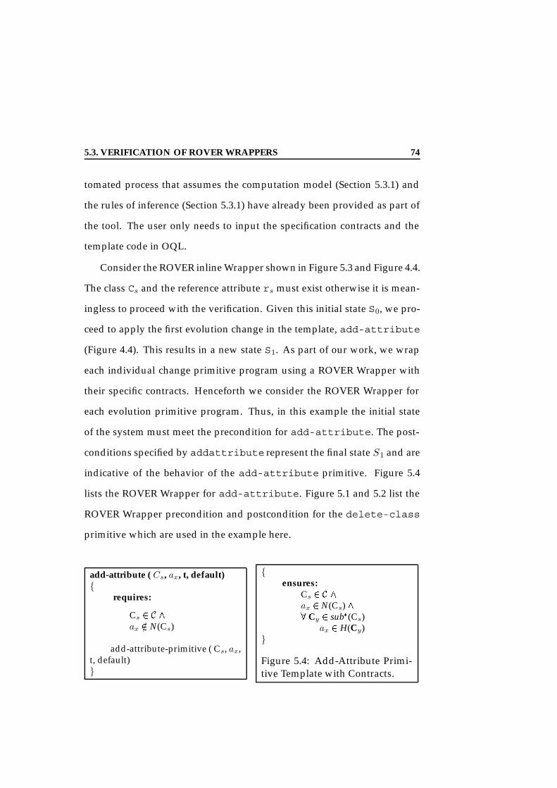
5.3. VERIFICATION OF ROVER WRAPPERS 74
tomated process that assumes the computation model (Section 5.3.1) and
the rules of inference (Section 5.3.1) have already been provided as part of
the tool. The user only needs to input the specification contracts and the
template code in OQL.
Consider the ROVER inline Wrapper shown in Figure 5.3 and Figure 4.4.
The class Cs and the reference attribute rs must exist otherwise it is mean-
ingless to proceed with the verification. Given this initial state S0, we pro-
ceed to apply the first evolution change in the template, add-attribute
(Figure 4.4). This results in a new state S1. As part of our work, we wrap
each individual change primitive program using a ROVER Wrapper with
their specific contracts. Henceforth we consider the ROVER Wrapper for
each evolution primitive program. Thus, in this example the initial state
of the system must meet the precondition for add-attribute. The post-
conditions specified by addattribute represent the final state S1 and are
indicative of the behavior of the add-attribute primitive. Figure 5.4
lists the ROVER Wrapper for add-attribute. Figure 5.1 and 5.2 list the
ROVER Wrapper precondition and postcondition for the delete-class
primitive which are used in the example here.
add-attribute ( Cs, ax, t, default)
requires:
Cs 2 C ^
ax /2 N(Cs)
add-attribute-primitive ( Cs, ax,t, default)
ensures:
Cs 2 C ^
ax 2 N(Cs) ^8 Cy 2 sub(Cs)
ax 2 H(Cy)
Figure 5.4: Add-Attribute Primi-tive Template with Contracts.

5.3. VERIFICATION OF ROVER WRAPPERS 75
A subsequent evolution change, add-attribute, uses this state S1
as its initial state against which its precondition must match. Tables 3.4
contains the schema evolution operations that we consider as rules of in-
ference in our system. The theorem prover proves the correctness of the
inline transformation shown in Figure 4.4 by first proving three theorems
where each theorem is similar to the add-attribute and then composes
them together to prove the correctness of the inline transformation itself
(the fourth theorem). Each of the theorems specifies the properties of one
of the evolution programs in the inline transformation.
Schema Evolution Primitive: add-attribute. The preconditions and post-
conditions from the contract specification in Figure 5.3 that must hold for
add-attribute(Cs, ax, type, default) are given in Equation 5.14:
Cs 2 C ^
ax /2 N(Cs)
(5.1)
The desired postconditions expected after applying add-attribute are:
Cs 2 C ^
σ(Cs) 2 types(C) ^
ax 2 N(Cs) ^
8y 2 sub(Cs)ax 2 H(y)
9>>>>>>=>>>>>>;
(5.2)
Theorem 3 If the add-attribute template is applied to arguments satisfy-
ing the precondition given in Equation 5.1, then the program results satisfy the
4These are repeated from Figure 5.3 for convenience.

5.3. VERIFICATION OF ROVER WRAPPERS 76
postcondition given in Equation 5.2.
Proof: Assume that the precondition in Equation 5.1 holds and add-attri-
bute adds the attribute ax to the class Cs (Table 3.5), i.e.:
N(Cs) = ax [ N(Cs)
(5.3)
The primitive add-attribute also adds ax to all the subclasses sub(Cs)
of Cs (refer Table 3.4). Hence we have:
8Cy 2 sub(Cs)H(Cy) = ax
[ H(Cy)
9=; (5.4)
Here Equations 5.3 and 5.4 show the altered states of the system after the
execution of each add-attribute function. From Equations 5.3 and 5.4,
we have the desired postcondition as specified in Equation 5.2. 2
In Figure 4.4, theforall loop copies all the attributes of the class CrefClass5.
At the end of the forall loop, with repetitive application of add-attri-
bute, the desired state is given by the postcondition in Equation 5.5.
Cs 2 C ^
σ(Cs) 2 types(C) ^
8ak 2 N(CrefClass)(ak 2 N(Cs)) ^
8Cy 2 sub(Cs)(ak 2 H(Cy))
9>>>>>>=>>>>>>;
(5.5)
Theorem 4 If the add-attribute function is correct as per Theorem 3, then
5CrefClass is the class that is being referred to by the reference attribute rx in class Cs.

5.3. VERIFICATION OF ROVER WRAPPERS 77
repetitive execution of add-attribute for all ak 2 CrefClass results in a cu-
mulative effect such that postcondition given in Equation 5.5 are satisfied.
Proof: (Proof By Induction)
Base Case: Assume that the class CrefClass has only one attribute a. This
reduces the for all statement to a simple add-attribute (Cs, a,
a.attrType, a.defaultValue). We know by Theorem 3 that if the
pre-condition given in Equation 5.1 holds for these arguments, then the
postcondition as given in Equation 5.2 will also hold, i.e., for one attribute
(n = 1), postcondition in Equation 5.5 reduce to postcondition in Equa-
tion 5.2.
Induction Hypothesis: Assume that the theorem holds true when class
CrefClass has k attributes and they are added to class Cs, i.e., the postcondi-
tion given in Equation 5.5 is satisfied for k add-attribute applications.
Induction: Prove that the post-condition in Equation 5.5 holds when the
class CrefClass has k+1 attributes.
We know that the postcondition (5.5) holds when class CrefClass has k
attributes and they are added to the class Cs. Assume we now have at-
tribute ak+1, the k + 1th attribute, that is unique, i.e., a k+1 6= aj , for 1
j k. To add this to class Cs we do: add-attribute(Cs, ak+1,
ak+1.attrType, ak+1.defaultValue). We know by Theorem 3 that if
this satisfies the precondition given in Equation 5.1, then the postcondition
in Equation 5.2 holds true (Base Case). Combining the postcondition for
the addition of k attributes (Induction Hypothesis) with the postcondition
of the Base Case, we get the postcondition as given in Equation 5.5. 2

5.3. VERIFICATION OF ROVER WRAPPERS 78
Schema Evolution Primitive delete-attribute. First we give the initial state
of the system, i.e., the precondition in Equation 5.6 that must be satisfied
for the primitive delete-attribute(Cs, ax):
Cs 2 C ^
ax 2 N(Cs)
(5.6)
After the execution of delete-attribute, the final state of the system is
as given in the postcondition in Equation 5.7.
ax /2 N(Cs) ^
8Cy 2 sub(Cs)ax /2 H(Cy)
9=; (5.7)
Theorem 5 If delete-attribute is applied to arguments satisfying precon-
dition (5.6), then the result satisfies the postcondition (5.7).
Proof: Similar to Theorem 3.
Schema Evolution Primitive delete-class. The necessary precondition that
must hold for delete-class(CrefClass) is given in Equation 5.8:
CrefClass 2 C ^
sub(CrefClass) = ; ^
in-degree(CrefClass) = 0 ^
(8oi 2 extent(CrefClass) : (obj-in-degree(oi) = 0))
9>>=>>;
(5.8)
The desired postcondition (5.9) after the application of delete-class is
as given in Equation 5.9.

5.3. VERIFICATION OF ROVER WRAPPERS 79
8 < Cx, rx > 2 out-paths(CrefClass)(< CrefClass > /2 in-paths(Cx)) ^
8Cx 2 super(CrefClass)(CrefClass /2 sub(Cx)) ^
CrefClass /2 C ^
σ(CrefClass) /2 types(C)
9>>>>>>=>>>>>>;
(5.9)
Theorem 6 If delete-class is applied to arguments satisfying the precondi-
tion in Equation 5.8, then the result satisfies the postcondition in Equation 5.9.
Proof: Similar to Theorem 3.
The Inline Transformation. To verify the correctness of the inline trans-
formation, we chain the results of Theorems 3, 4, 5 and 6. The overall
precondition for this is given by Equation 5.106. The execution of the inline
transformation must result in the final state as specified by Equation 5.117.
Cs 2 C ^
ax 2 N(Cs) ^
CrefClass = domain(ax) ^
CrefClass 2 C ^
Cs 6= CrefClass
9>>>>=>>>>;
(5.10)
Cs 2 C ^
CrefClass /2 C ^
8ak 2 N(CrefClass)(ak 2 N(Cs)) ^
8Cy 2 sub(Cs)(ak 2 H(Cy) ^
ak /2 N(Cs))
9>>>>>>>>=>>>>>>>>;
(5.11)
6This is the precondition for the inline wrapper in Figure 5.3.7This is the postcondition for the inline wrapper given in Figure 5.3.

5.4. SUMMARY 80
Theorem 7 If Theorems 3, 4, 5, and 6 are satisfied in the order specified, then the
inline transformation satisfies the postcondition given in Equation 5.11.
Proof: The proof for this can be given by a combination of the postcondition
in Equations 5.5, 5.7 and 5.9. 2
Using theorem proving techniques as shown for the template here it
is possible to verify the correctness of any given template. If at any point
one of the sub-theorems is not satisfied, i.e., if Theorem 3, 4, 5, or 6 is
not satisfied, the verification process will be aborted and the template not
permitted to execute. However, all of this will occur prior to any execution
of the ROVER Wrapper. Hence, any failure of the verification process will
result in no execution of the ROVER Wrapper. While such a verification
process may incur additional overhead of checking, we believe it can be
shown that under erroneous conditions the verification process can save
hours when compared to a roll-back strategy.
5.4 Summary
In this chapter, we have addressed the issue of consistency of the DBMS
systems after the execution of complex transformations such as a SERF
transformation. We have defined two levels of consistency, invariant pre-
serving, that ensures that after the execution of a SERF template, the re-
sultant OODB database conforms to the invariants of the data model. We
have shown show that that if each schema evolution operation is an in-
variant preserving operation, then a SERF template is also invariant pre-
serving [CRed]. Within the context of SERF, we have identified the need to

5.4. SUMMARY 81
define template semantic consistency that would allow users to specify con-
sistency requirements for their templates. To enable users to specify these
template-semantic constraints, we have introduced the notion of Template
Wrappers [CRH00b]. These Template Wrappers, based on Software Con-
tracts [Mey92], allow a user to specify semantic constraints on a template
which can then be checked at runtime. Such contracts can also be checked
prior to the execution of the template. We have shown via an example that
theorem-provers may be a feasible option in this area [CRH01].

5.4. SUMMARY 82

83
Chapter 6
Reducing the Runtime of SERF
Templates
In this chapter we look at reducing the run-time of SERF templates. Specif-
ically, we look at reducing the run-time of a template. For this we present
the CHOP approach [CNR00, CNR99]1.
6.1 Optimizing the Performance of Schema Evolution
Sequences
Schema evolution is an expensive process both in terms of system resource
consumption as well as database unavailability [FMZ94b]. This expense of
schema evolution is further emphasized by now having complex evolution
operations that string multiple primitive schema evolution operations in a
1This work was done in collaboration with Chandrakant Natarajan, a Master’s studentat WPI.

6.1. OPTIMIZING THE PERFORMANCE OF SCHEMA EVOLUTIONSEQUENCES 84
sequence as in the case of SERF templates. As a first step of optimization,
we present an approach that disregards the queries and instead focuses on
reducing the run-time execution of just the schema evolution operations.
In previous work, researchers have looked at improving system avail-
ability during schema evolution by proposing execution strategies such as
deferred execution [Tec94, FMZ94b]. No work, however, has been under-
taken to actually optimize or reduce the sequence of operations that are
being applied to a given schema. Kahler et al. [KR87] have looked at pre-
execution optimization for reducing the number of update messages that
are sent to maintain replicated sites in the context of distributed databases.
In their approach, the messages are simple data updates on tuples. The
messages are sorted by their tuple-identifier, and then the change history
of the tuple is condensed (with merge or remove) into one update opera-
tion.
We now present a similar approach (merge, cancel, eliminate) for op-
timizing a sequence of schema evolution operations. Our approach is or-
thogonal to the existing execution strategies for schema evolution, i.e., it
can in fact be applied to both immediate and the deferred execution strate-
gies [FMZ94b]. The optimization strategy, called CHOP, exploits two prin-
ciples of schema evolution execution within one integrated solution:
• Minimize the number of schema evolution operations in a sequence
by canceling or eliminating schema evolution operations. For exam-
ple, adding an attribute and then deleting the same attribute is an
obvious case of cancellation where neither operation needs to be exe-

6.1. OPTIMIZING THE PERFORMANCE OF SCHEMA EVOLUTIONSEQUENCES 85
cuted.
• Merge the execution of all schema evolution changes that operate
on one extent to amortize the cost of schema evolution over several
schema changes. For example, consider a sequence that adds two
or more attributes to the same class. Object updates for these done
simultaneously can potentially reduce the cost of executing these se-
quentially by 50%.
In this section we present a general strategy for reducing a given se-
quence of schema evolution operations prior to its actual execution. Our
work is based on a taxonomy of schema evolution operations we devel-
oped for the ODMG object model as given in Table 3.2.2 but it can easily
be applied to any other object model. We present here an analysis of the
schema evolution operations and the schema to characterize the conditions
under which operations in a sequence can be optimized. Based on this anal-
ysis we present the merge, cancel and eliminate optimization functions and
the conditions under which they can be applied. We have also been able
to show both formally and experimentally that the order in which these
functions are applied is not relevant for the final optimized sequence, i.e.,
they will all produce the same unique final sequence. As a conclusion to our
work we also present a summary of our experimental results.
6.1.1 Foundations of Schema Evolution Sequence Analysis
To establish a foundation for our optimization principles we have devel-
oped a formal characterization of the schema evolution operations, their

6.1. OPTIMIZING THE PERFORMANCE OF SCHEMA EVOLUTIONSEQUENCES 86
impact on the schema, as well as their interactions within a sequence.
Term Description Capacity Effectsadd-class(c, C) Add new class c to C in
schema S (AC)augmenting
delete-class(c) Delete class c from C
in schema S if sub-classes(C) = ; (DC)
reducing
rename-class(c, d) Rename class c to d(CCN)
preserving
add-ISA-edge(cx , cy) Add an inheritanceedge from cx to cy(AE)
augmenting
delete-ISA-edge(cx , cy) Delete the inheritanceedge from cx to cy(DE)
reducing
add-attribute(cx , ax, t, d) Add attribute ax oftype t and defaultvalue d to class cx(AA)
augmenting
delete-attribute(cx , ax) Delete the attribute axfrom the class cx (DA)
reducing
rename-attribute(ax , bx, cx) Rename the attributeax to bx in the class cx(CAN)
preserving
Table 6.1: The Taxonomy of Schema Evolution Primitives.
Schema evolution operations are generally categorized as capacity-aug-
menting if they increase the capacity of the schema, for instance, by adding
a class, capacity-reducing if they decrease the capacity of the schema, for
instance, by deleting a class, or capacity-preserving if they do not change
the capacity of the schema, for instance, by changing the name of a class
[RR97]. For each schema evolution primitive its capacity type is shown in
the third column of Table 6.1.

6.1. OPTIMIZING THE PERFORMANCE OF SCHEMA EVOLUTIONSEQUENCES 87
Table 6.2 defines the various relationships that can exist in general be-
tween schema evolution operations. Table 6.3 applies these to the schema
evolution operation presented in Table 6.1.
Operation Relation Descriptionsame-operation-as op1 is same-operation-as op2 if they both have the same op-
eration name irrespective of the particular parameters theyare being applied to.
inverse-operation-of op1 is inverse-operation-of op2 if the effects of one opera-tion op1 could be canceled (reversed) by the effects of theother operation op2.
super-operation-of op1 is super-operation-of op2 if the functionality of op1 su-percedes the functionality of op2, i.e., op1 achieves as part ofits functionality also the effects of op2
Table 6.2: Classification of Operation Properties.
AC() DC() CCN() AA() DA() CAN() AE() DE()AC() same inverse - super - - - -DC() inverse same super super super super super superCCN() - - same
in-verse
- - - - -
AA() - - - same inverse - - -DA() - - - inverse same super - -CAN() - - - - - same - -AE() - - - - - - same inverseDE() - - - - - - inverse same
Table 6.3: Classification of Operation Properties for the Schema EvolutionTaxonomy in Table 3.4 (with same = same-operation-as, inverse = inverse-operation-of and super = super-operation-of).
However, for optimization it is not sufficient to categorize the schema
evolution operations based on just their functionality. It is important to
also know the parameters, i.e., the context in which these operations are
applied. Table 6.4 presents the schema element relationships.
While the operation properties (Table 6.2) and the context properties (Ta-
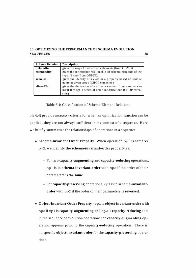
6.1. OPTIMIZING THE PERFORMANCE OF SCHEMA EVOLUTIONSEQUENCES 88
Schema Relation DescriptiondefinedIn gives the scope for all schema elements (from ODMG).extendedBy gives the inheritance relationship of schema elements of the
type Class (from ODMG).same-as gives the identity of a class or a property based on unique
name in given scope (CHOP extension).aliasedTo gives the derivation of a schema element from another ele-
ment through a series of name modifications (CHOP exten-sion).
Table 6.4: Classification of Schema Element Relations.
ble 6.4) provide necessary criteria for when an optimization function can be
applied, they are not always sufficient in the context of a sequence. Here
we briefly summarize the relationships of operations in a sequence.
• Schema-Invariant Order Property. When operation op1 is sameAs
op2, we identify the schema-invariant-order property as:
– For two capacity-augmenting and capacity-reducing operations,
op1 is in schema-invariant-order with op2 if the order of their
parameters is the same.
– For capacity-preserving operations, op1 is in schema-invariant-
order with op2 if the order of their parameters is reversed.
• Object-Invariant-Order Property - op1 is object-invariant-order with
op2 if op1 is capacity-augmenting and op2 is capacity-reducing and
in the sequence of evolution operations the capacity-augmenting op-
eration appears prior to the capacity-reducing operation. There is
no specific object-invariant-order for the capacity-preserving opera-
tions.

6.1. OPTIMIZING THE PERFORMANCE OF SCHEMA EVOLUTIONSEQUENCES 89
• Dependency Property - The schema elements used as parameters
by the two operations op1 and op2 being considered for optimiza-
tion must not be referred to by any other operation which is placed
between the two operations in the sequence.
6.1.2 The CHOP Optimization Functions
The integral component of the CHOP optimization algorithm are the op-
timization functions that can be applied to pairs of schema evolution op-
erations within the context of their resident schema evolution operation
sequence. In this section we present the general description of an optimiza-
tion function and three instantiations of the optimization functions (merge,
cancel and eliminate), that we have formulated for the optimization of the
primitive set of schema evolution operations given in Section 3.2.2.
An Optimization Function
The crux of the CHOP optimization algorithm is an optimization function
which takes as input two schema evolution operations and produces as
output zero or one schema evolution operation, thereby reducing the se-
quence of the schema evolution operations. Formally, we define an opti-
mization function as follows:
Definition 1 Given a schema evolution operation sequence Σ, hop1, op2 . . .
opni with opi before opj 1 i j n, an optimization function FΣ produces
as output an operation op which replaces opi. The operation at index position j
is set to a no-op. The operations op, opi and opj are either schema evolution

6.1. OPTIMIZING THE PERFORMANCE OF SCHEMA EVOLUTIONSEQUENCES 90
primitives as described in Table 6.1 or complex evolution operations as defined in
Section 6.1.2.
A major requirement for the CHOP optimization is to reduce the num-
ber of schema evolution operations in a sequence such that the final schema
produced by this optimized sequence is consistent and is the same as the
one that would have been produced by the unoptimized sequence for the
same input schema. Thus, an optimization function must not in any way
change the nature of the schema evolution operations or the order in which
they are executed. Towards that goal, any optimization function must ob-
serve several properties we now list.
Invariant-Preserving-Output Operations. Schema evolution operations
guarantee the consistency of the schema and the database by preserving the
invariants defined for the underlying object model [BKKK87]. An impor-
tant property of the optimization function therefore is for its output (any of
its output operations) to also preserve the schema consistency by preserv-
ing the invariants defined for the object model.
Schema-State Equivalent. Above all an optimization function must guar-
antee correctness, i.e., the schema produced by output of the optimization
function (optimized sequence) must be the same as the schema produced
by the unoptimized sequence when applied to the same input schema. This
property can in fact be proven formally (refer [CNR99]).

6.1. OPTIMIZING THE PERFORMANCE OF SCHEMA EVOLUTIONSEQUENCES 91
Relative-Order Preserving. As discussed in Section 6.1.1, the order in
which the schema evolution operations appear with respect to one another
in a sequence is relevant to the application of an optimization function. This
relative order of an operation opi in a sequence is defined by its index, i,
with respect to the index of the other operations. For example, if i < j,
then opi is before opj in the sequence, denoted by opi < opj . Operations
executed out-of-order can cause unexpected variance in the final output
schema. For example, consider two operations in a sequence with the order
as given here: < DA(C,a), AA(C,a)>. When executed in the order given
the attribute a is first deleted from the class C and then re-added. However,
all of the information stored in the attribute a is lost. Now, switching the
order of execution of the two operations leads to a very different schema.
Thus, it is essential for an optimized sequence to preserve the relative-
order of the input sequence.
Using the above stated properties, we now refine the definition of an opti-
mization function as follows:
Definition 2 (Optimization Function.) Any optimization function in CHOP
defined as in Definition 1 must be invariant-preserving, schema-state-equi-
valence preserving and relative-order preserving.
For the CHOP approach, we define three such optimization functions, Merge,
Eliminate, and Cancel.

6.1. OPTIMIZING THE PERFORMANCE OF SCHEMA EVOLUTIONSEQUENCES 92
The Merge Optimization Function
The time taken for performing a schema evolution operation is largely de-
termined by the page fetch and page flush times [FSS+97]. In our proposed
CHOP approach we amortize the page fetch and flush costs over several
operations by collecting all transformations on the same set of objects and
performing them simultaneously 2.
A complex operation denoted by < op1, .... opk > with k 2
is defined as a collection of schema evolution operations for the same class
which affect the same set of objects, i.e., it is possible to perform all the
object transformations for these operations during the same page fetch and
flush cycle. For two complex operations, op1 = < opi.... opj > and
op2 = < opm.... opn >, the operation pairs (opj,opm) and (opn,
opi) are termed complex-representative pairs.
Definition 3 Merge is an optimization function (Definition 2) that takes as in-
put a pair of schema evolution operations, either primitive or complex, op1 and
op2, and produces as output a complex operation op3 = < op1, op2 >. If
one or both of the input operations are a complex operation, e.g., op1 = <opi,
. . . opj > and op2 = <opm, . . . opn >, then a relative order within the com-
plex operations op3 is maintained such that the output operation op3 = <opi,
. . ., opj, opm, . . ., opn >. The input operations op1 and op2 must sat-
isfy:
• Context Property2This merge of operations relies on the underlying OODB system to be able to separate
the schema evolution operation into a schema change at the Schema Repository level andinto object transformations at the database level.

6.1. OPTIMIZING THE PERFORMANCE OF SCHEMA EVOLUTIONSEQUENCES 93
– If op1 and op2 are related by the same-operation-as property, then
their context parameters must be definedIn same scope.
– If op1 and op2 are related by the super-operation-of property, then
for the sub-operation the definedIn scope of the context must be the
sameAs the context of the super-operation.
– If op1 and op2 are related by the inverse-operation-of property,
then the context of op1 must be sameAs the context of op2 and de-
finedIn same scope.
• Dependency Property must hold.
When one or both of the input operations op1 and op2 are complex, then all
the merge conditions given above must be satisfied by at least one pair of operations
in the complex operation. This is the complex-representative pair and enforces
the an ordering of the complex operation.
For example, given an operation that adds a name attribute to a class
called Employee and a subsequent operation that adds a age attribute
to the same class Employee, we can merge the two operations they are
related by the same-operation-as property and their context parameters
are definedIn the same scope, i.e., Employee for both operations is in the
same schema and the attributes name and age are being added to the same
class Employee. Lastly, the dependency property holds as there are no
operations between the index positions of the two operations.
A complex operation is thus a sub-sequence of schema evolution oper-
ations and other optimization functions (cancel and eliminate) can be ap-

6.1. OPTIMIZING THE PERFORMANCE OF SCHEMA EVOLUTIONSEQUENCES 94
plied on the primitive schema evolution operations inside of a complex op-
eration. However, the merge optimization function itself cannot be applied
inside a complex operation to prevent infinite recursion.
The Eliminate Optimization Function
In some cases a further optimization beyond merge may be possible. For
example, while it is possible to mergeDA(Employee, name) and DC(Emp-
loyee) the execution of DC(Employee) makes the prior execution of
DA(Employee, name) redundant. Hence, some operations may be op-
timized beyond a merge by being completely eliminated by other opera-
tions, thus reducing the transformation cost by one operation.
Definition 4 Eliminate is an optimization function as defined in Definition 2
that takes as input a pair of schema evolution primitives op1 and op2 and pro-
duces as output op3, such that op3 = op1 if op1 = super-operation-of (op2)
or op3 = op2 if op2 = super-operation-of (op1). The input operations op1
and op2 must satisfy:
• Operation Property such that either op1 = super-operation-of (op2)
or op2 = super-operation-of (op1),
• Context Property such that the definedIn scope of the sub-operation is
sameAs the context parameter of the super-operation, and
• Dependency Property must hold.

6.1. OPTIMIZING THE PERFORMANCE OF SCHEMA EVOLUTIONSEQUENCES 95
The Cancel Optimization Function
In some scenarios further optimization beyond a merge and eliminate may
be possible. Some schema evolution operations are inverses of each other,
for example, AA(Employee, age) adds an attribute and DA(Employee,
age) removes that attribute. A cancel optimization thus takes as input two
schema evolution operations and produces as output a no-op operation,
i.e., an empty operation that does nothing.
Definition 5 Cancel is an optimization function as in Definition 2 which takes
as input a pair of schema evolution primitives op1 and op2 and produces as out-
put op3, where op3= no-op, an empty operation, assuming the input operations
op1 and op2 satisfy:
• Operation Property such that op1 and op2 are related by the inverse-
operation-of property,
• Context Property such that op1 and op2 are definedIn the same scope
and op1 is sameAs op2,
• Schema-Invariant-Order Property for capacity-reducing operations must
hold,
• Object-Invariant-Order Property must hold, and
• Dependency Property must hold.
6.1. OPTIMIZING THE PERFORMANCE OF SCHEMA EVOLUTIONSEQUENCES 96
6.1.3 CHOP Optimization Strategy
The CHOP optimization algorithm iteratively applies the three classes of
optimization functions merge, eliminate and cancel introduced in Section
6.1.2 until the algorithm terminates and a minimal solution is found.
However, before we can address the issue of minimality it is necessary
to examine two issues: (1) if one or more functions are applicable, is choos-
ing the right function essential? and (2) when there are more than one pair
of operations that can be optimized, is choosing the right pair essential?
Choosing the Right Optimization Function. We note that the conditions
under which the merge optimization function can be applied is a superset of
the conditions under which an eliminate or a cancel can be applied, while
the conditions under which a cancel and an eliminate can be applied are
mutually exclusive. Thus, often a merge can be applied to a pair of op-
erations where either an eliminate or a cancel can be also applied. How-
ever, as these optimizations offer different degrees of reduction for a pair of
schema evolution operations (with merge offering the least and cancel the
most), choosing the optimization function that offers the most reduction is
desirable.
We can however formally show that doing a merge where a cancel or
an eliminate is also applicable does not prevent the application of a cancel
or an eliminate during the next iterative application of these functions. A
formalization of this property and its proof is given in [CNR00].

6.1. OPTIMIZING THE PERFORMANCE OF SCHEMA EVOLUTIONSEQUENCES 97
Operation Dependencies and Optimization Functions. An important cri-
teria for the successful application of any of the three optimization func-
tions is that the Dependency Property as given in Section 6.1.1 must hold.
That is, there must be no reference to the schema elements used as param-
eters in the two operations op1 and op2 being considered for optimiza-
tion by any other operation which is placed between the two operations
in the sequence. However, the order in which the pairs of operations are
selected can have an effect on this dependency.
Consider a sequence of three operations op1, op2 and op3. Con-
sider that the pairs (op1, op2) and (op2, op3) can be immediately opti-
mized while a successful optimization of the pair (op1,op3) requires re-
moving the dependency operation op2. In this case, there are two possibil-
ities for applying the optimization functions on the pairs of operations. We
could either apply the respective optimization functions on the pair (op1,
op2) and then on the pair (op2, op3) 3 and not be concerned about the
optimization possibility between op1and op3. Or we could first apply the
optimization function on the pair (op2, op3), reduce the dependency op2
and then optimize the pair (op1, op3). However, as before our goal is to
achieve the maximum optimization possible.
We can formally show that the order of selection for pairs of schema
evolution operations in a sequence for the application of one of the three
optimization functions does not prevent the achievement of maximum op-
timization [CNR99].
3Note that in some cases op2may not exist any more and hence optimizing (op2, op3)may no longer be possible.

6.1. OPTIMIZING THE PERFORMANCE OF SCHEMA EVOLUTIONSEQUENCES 98
Confluence. While the main goal for the optimization is to achieve max-
imum optimization possible in an effort to reduce schema evolution costs,
we also want to keep the overhead of optimizing to a minimal. How-
ever, there are multiple permutations and combinations of the optimization
functions and the pairs of schema evolution operations that can potentially
achieve the maximum optimization. Enumerating all the possible choices
prior to selecting one for execution results in an exponential search space.
This overhead from enumerating these choices alone would cancel any po-
tential savings achieved by the optimization.
However, based on the function properties in [CNR99], we can show
that all possible combinations of optimization functions for a given se-
quence converge to one unique minimal, thereby eliminating the need to
enumerate all the possible choices. The following states the theorem of
confluence. The proof for this is given in [CNR99].
Theorem 8 [Confluence Theorem]: Given an input schema evolution sequence,
Σin, all applicable combinations of optimization functions fi produce minimal re-
sultant sequences Σi that are identical.
6.1.4 Experimental Validation
We have conducted several experiments to evaluate the potential perfor-
mance gains of the CHOP optimizer. Our experimental system, CHOP, was
implemented as a pre-processing layer over the Persistent Storage Engine
(PSE Pro2.0). All experiments were conducted on a Pentium II, 400MHz,
128Mb RAM running WindowsNT and Linux. We used a payroll schema
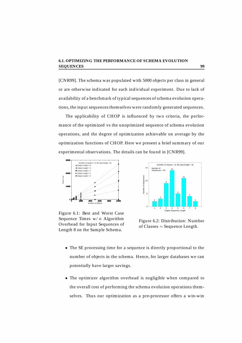
6.1. OPTIMIZING THE PERFORMANCE OF SCHEMA EVOLUTIONSEQUENCES 99
[CNR99]. The schema was populated with 5000 objects per class in general
or are otherwise indicated for each individual experiment. Due to lack of
availability of a benchmark of typical sequences of schema evolution opera-
tions, the input sequences themselves were randomly generated sequences.
The applicability of CHOP is influenced by two criteria, the perfor-
mance of the optimized vs the unoptimized sequence of schema evolution
operations, and the degree of optimization achievable on average by the
optimization functions of CHOP. Here we present a brief summary of our
experimental observations. The details can be found in [CNR99].
0 2000 4000 6000 8000 10000Number of Objects
0
10000
20000
30000
Tim
e in
ms
Output Length = 8
0 2000 4000 6000 8000 100000
10000
20000
30000
Output Length = 6
0 2000 4000 6000 8000 100000
10000
20000
30000
Output Length = 4
0 2000 4000 6000 8000 100000
10000
20000
30000
Output Length = 2
0 2000 4000 6000 8000 100000
10000
20000
30000
Output Length = 0
Number of classes = 8; SE input length = 8)
Figure 6.1: Best and Worst CaseSequence Times w/o AlgorithmOverhead for Input Sequences ofLength 8 on the Sample Schema.
1 2 3 4 5 6 7 8Output Sequence Length
0
5
10
15
Num
ber
of S
eque
nces
23
9
14
5
11
4
2
Number ofSequences = 50
(number of classes = 8; SE input length = 8)
Figure 6.2: Distribution: Numberof Classes = Sequence Length.
• The SE processing time for a sequence is directly proportional to the
number of objects in the schema. Hence, for larger databases we can
potentially have larger savings.
• The optimizer algorithm overhead is negligible when compared to
the overall cost of performing the schema evolution operations them-
selves. Thus our optimization as a pre-processor offers a win-win

6.2. SUMMARY 100
solution for any system handling sequences of schema changes (Fig-
ure 6.1).
• The degree of optimization increases with the increase in the number
of class-related operations in the sequence. Hence, depending on the
type of sequence, major improvements are possible (Figure 6.2).
• A random application of the optimization functions on the same se-
quence resulted in the same final sequence of schema evolution oper-
ations.
• We have experimentally tested that on a small-sized database of 20,000
objects per class, even the removal of a single schema evolution op-
eration on a class already results in a time saving of at least 7000 ms.
This time savings is directly proportional to the number of attributes
and the extent size of a class thus offering huge savings for today’s
larger and larger database applications.
6.2 Summary
In this chapter we have presented the first optimization strategy for schema
evolution sequences. CHOP minimizes a given schema evolution sequence
through the iterative elimination and cancellation of schema evolution prim-
itives on the one hand and the merging of the database modifications of
primitives on the other hand. Important results of this work are the proof
of correctness of the CHOP optimization, a proof for the termination of the
iterative application of these functions, and their convergence to a unique
6.2. SUMMARY 101
and minimal sequence. We have performed experiments on a prototype
system that clearly demonstrate the performance gains achievable by this
optimization strategy. For random sequences an average optimization of
about 68% was achieved.
CHOP in its current form does not take into account the presence of
OQL queries that are an inherent part of the a SERF template. This is a
potential future work project that would extend the basic techniques that
we have presented here.

6.2. SUMMARY 102

103
Chapter 7
Design and Implementation of
the OQL-SERF System
In this section we present a brief overview of our implementation of the
SERF Framework - OQL-SERF. A more detailed description can be found
in [CJR98b]. OQL-SERF, a Java-based system is built using Object Design
Inc.’s Persistent Storage Engine Pro 2.0 (PSE Pro 2.0) as the underlying
OODB system [O’B97]. It uses the JDK 1.2 and has been implemented and
tested on Windows NT and Linux (S.U.S.E 6.3). It is based on the ODMG
standard. In particular, we used an extension of Java’s ODMG binding and
our own Java binding of the ODMG Schema Repository. A prototype of
this system was demonstrated at SIGMOD 1999 [RCL+99].

7.1. SYSTEM ARCHITECTURE 104
7.1 System Architecture
Figure 7.1 presents the system design for OQL-SERF. PSE, a lightweight
OODB written in Java [O’B97], has been chosen for SERF due to its porta-
bility to different platforms, the availability of a free version and its confor-
mance to the Java ODMG binding.
SERF Framework
OODB System
QueryEngine
SchemaRepository
SchemaEvolutionPrimitives
ObjectRepository
queries
queries
operates on
TemplateProcessor
Instantiates and executes
Template Manager
UserInterface
SchemaViewer
TemplateEditor
uses
uses
uses uses
TemplateLibrary
Figure 7.1: Architecture of the SERF Framework
In a persistent storage system, such as PSE, it is assumed that the schema
representation, data, applications and the links between them are all held
as objects in persistent storage. While PSE offers most OODB features, it
does not explicitly define a Schema Repository as per the ODMG standard.
It also does not have the requisite schema evolution support and its query

7.2. SERF FRAMEWORK MODULES 105
interface does not meet the requirements of a query language for SERF.
Thus as part of the OQL-SERF implementation, we have addressed
these limitations and built:
• A fully operational ODMG compliant Schema Repository.
• A complete schema evolution facility that preserves the ODMG object
model and does changes at a finer granularity, thus allowing for in-
place evolution.
• An OQL Query Engine for querying the objects in PSE.
In the future we would expect an underlying OODB realizing SERF to
provide these basic capabilities. In this section we hence do not go into the
details of the above extensions (see [CJR98b]). Rather, we focus on describ-
ing the framework modules that are the core of SERF.
7.2 SERF Framework Modules
The SERF Framework Modules are the core components that need to be
provided by any system realizing the SERF Framework. Sections 7.2.1 and
7.2.3 describe the functionality and support needed for SERF templates and
transformations.
7.2.1 Template Module
The Template Module provides all of the functionality for storing, retriev-
ing and executing templates. Figure 7.2 shows the architecture for the Tem-
plate Module in OQL-SERF.

7.2. SERF FRAMEWORK MODULES 106
TemplateManager
TemplateLibrary
Provides APIs for storing and searchingtemplates
Type & BindChecker
Verifier
Executestemplates
Static and Bind time
TemplateProcessor
Figure 7.2: The Template Module.
Template
templateName;parameterList;sourcecode;description;keywords;
newTemplate();
editTemplate();
deleteTemplate();
executeTemplate();
Figure 7.3: The Template Class.
The Template Manager. The Template Manager is the public interface of
the template module. Through the template manager the user can retrieve,
edit and execute already existing templates as well as create and store new
templates.
The Template Processor. The Template Processor executes a template.
Figure 7.4 shows the steps, beginning with the user supplying the input
parameters. A type-check ensures that the types of the parameters match
and they exist in the system as well as the correct number of parameters
are supplied by the user. This is followed by a bind-check that checks the
existence of these actual parameters in the schema on which they are being
applied by accessing the Schema Repository. If the checks are successful,
the SERF template is instantiated using these parameters by replacing each
variable with its bound parameter. The instantiated template now corre-
sponds to pure OQL statements, i.e., we now call it an OQL transformation.
The OQL Query Engine provides an interface for the syntax-checking, the
parsing and the execution of the OQL transformation.

7.2. SERF FRAMEWORK MODULES 107
Figure 7.4: Steps for the Execution of a Template
7.2.2 Template Library
The SERF templates for a particular domain are collected in a Template
Library. A Template Manager at any given time can manage multiple Tem-
plate Libraries. For this reason libraryName.templateName gives the
complete path for storing and retrieving a template. Within a template li-
brary each template is represented by a corresponding template object 1, an
instance of the TemplateClass (see Figure 7.3). Each template object hence
contains a name, description, set of input parameters, list of keywords and oql
source for its template.
The Template Library currently provides the users (via the Template
Manager) the capability to search for a template in the library via simple
keyword search on all stored parameters of the template such as the input
and output parameters, the name, and the description.
1We distinguish between a template and a SERF template. Here a template object impliesan instance of the TemplateClass and a SERF template is the source code that is part of thisinstance.

7.2. SERF FRAMEWORK MODULES 108
7.2.3 User Interface
For OQL-SERF version 1.0, we have designed a graphical user interface
(GUI) as a front-end to the Template Manager. It provides a Template Ed-
itor with syntax highlighting that allows the user to create a new or edit
an existing template as shown in Figure 7.5. The Save option walks the
user through the steps of providing the name, list of formal parameters, de-
scription, and keywords for the SERF template object before it can be stored
and managed by the template library. It also provides a graphical interface
for viewing, searching and retrieving the templates stored in the Template
Library. The GUI allows the user to utilize a schema viewer to select the
parameters for instantiating a template (see Figure 7.6). The user can then
view the schema graph before and after a transformation has been applied
to the schema thus giving the user a chance to verify if this was indeed the
desired transformation.
Figure 7.5: The Template Editor. Figure 7.6: The Schema Viewer.

7.3. SUMMARY 109
7.3 Summary
In this chapter we have presented the architecture and the implementation
details of our prototype system, OQL-SERF. This system was demonstrated
at SIGMOD99 [RCL+99]. The key advantage of this architecture is that
it provides enhanced schema evolution capabilities without requiring the
underlying system to change.

7.3. SUMMARY 110

111
Chapter 8
Case Study of Different
Schema Transformations
We have presented SERF as a system that gives users:
• Extensibility: Allows users to define new transformations so they are
not limited by one fixed taxonomy of schema evolution primitives
provided by the underlying OODB;
• Flexibility: Allows users to define semantics of their choice for a trans-
formation and does not limit them to the pre-defined semantics set
forth by the underlying OODB.
• Re-usability: Allows the users to move away from writing ad-hoc
programs for complex transformations and instead offers the users
re-usability of their OQL code via the templates as well as by building
templates composed of other templates.

8.1. THE MERGE TRANSFORMATION 112
Several researchers have looked at simple and complex schema trans-
formations in the context of schema evolution [Ler00, Bre96], schema inte-
gration [BLN86, MIR93], and re-structuring [BB99, DKE94, DK97] in gen-
eral. A large subset of these transformations involves changing more than
one class, such as inline which inlines two classes dependent on the ref-
erence attribute, or merge which combines two classes based on a variety
of criteria. We have been successful at modeling the transformations pro-
posed in prior works using SERF templates. The goal of the case study
presented here is to show that SERF transformations can not only handle
the transformations presented in literature (inline, encapsulate, split, merge-
union, merge-difference) but also capture different semantics specified by the
user. In this section we present the merge transformation and show how
a user can specify templates each with different semantics for creating the
merged class. We also present examples of templates that are now applied
for the re-structuring of web pages.
8.1 The Merge Transformation
Lerner [Ler00] defines merge as a compound type change involving type
deletion. Merging deletes two or more object types and creates a new type
that represents the integration of the deleted types [Ler00]. The seman-
tics of the merge, such as the attributes based on which the objects can be
combined, are built into the merge compound change. However, we note
that there are several different possibilities for the structural definition of
the new type as well as for its object creation. For example, the structure

8.1. THE MERGE TRANSFORMATION 113
of the new class can be defined by doing a union of the properties of the
two source classes or by an intersection of the attributes of the two classes.
Similarly, object creation can be specified by a Cartesian product, by a sim-
ple join of one single property or by possibly a more complex join. By
previous approaches in the literature focusing on complex transformations
[Bre96, Ler00], the merge has generally been defined as one fixed transfor-
mation. Below in our case study we first show how using templates we can
achieve the semantics as defined by them and then can apply new seman-
tics at both the structural level and the object transformation level flexibly
within SERF. In the merge transformation case study below we show three
different semantics for achieving the structural definition of the new class
(merge, difference, intersection) and then we will show two possibilities for
doing the object transformations for the merge transformation.
8.1.1 The Merge-Union Template
Figure 8.1 represents the semantics of the merge-union process using an
example. Here the structure of the new class MergePapers is defined by a
union of the properties of the two source classes Authors and the Papers.
Figure 8.3 shows the template that is used for creating the merge-union
class MergePapers. This template takes five parameters: the two source
classes; the name of the new class (merge-union) class; and the join op-
eration. In our example, creation of the new objects for the MergePapers
class is specified by the join of the Authors objects and the Papers objects
such that Authors.AuthorName = Papers.AuthorName.

8.1. THE MERGE TRANSFORMATION 114
Figure 8.1: Merge-Union: TheStructure of the New Class givenby Union of the Properties ofthe Two Source Classes Authors,Papers.
Figure 8.2: Merge-Difference: TheStructure of the New Class givenby Difference of the Properties ofthe Two Source Classes Authors,Papers.
8.1.2 The Merge-Difference Template
The Merge-Union template shows one possible semantic definition for the
structure of the new class. Another possible semantic for a merge is to cre-
ate a new class by taking a difference of the sets of properties of the two
given classes. That is, if a property exists in both of the given classes,
then it is not a property of the new class. Figure 8.2 pictorially repre-
sents the merge-difference semantics. Here the structure of the new class
MergePapers has the properties Email, Affiliation,Published and
Title, the difference set of the properties of the two source classesAuthors
and Papers. Figure 8.4 shows the template that is used for creating the
merge-difference class MergePapers. The object transformation for the
template is based on the same join pair as above.
It can be observed by comparing the templates that the only a few lines
of OQL code have been modified as marked in Figure 8.4. Thus in SERF
extensibility is often obtained with little effort.
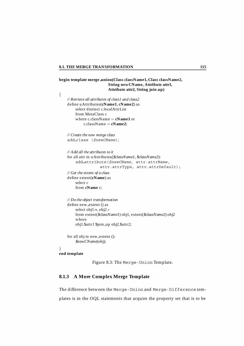
8.1. THE MERGE TRANSFORMATION 115
begin template merge union(Class className1, Class className2,String newCName, Attribute attr1,Attribute attr2, String join op)
// Retrieve all attributes of class1 and class2define uAttributes(cName1, cName2) as
select distinct c.localAttrListfrom MetaClass cwhere c.className = cName1 or
c.className = cName2;
// Create the new merge classadd class ($newCName);
// Add all the attributes to itfor all attr in uAttributes($className1, $className2):
add attribute($newCName, attr.attrName,attr.attrType, attr.attrDefault);
// Get the extent of a classdefine extent(cName) as
select cfrom cName c;
// Do the object transformationdefine new extent () as
select obj1., obj2.from extent($className1) obj1, extent($className2) obj2whereobj1.$attr1 $join op obj2.$attr2;
for all obj in new extent ():$newCName(obj);
end template
Figure 8.3: The Merge-Union Template.
8.1.3 A More Complex Merge Template
The difference between the Merge-Union and Merge-Difference tem-
plates is in the OQL statements that acquire the property set that is to be

8.1. THE MERGE TRANSFORMATION 116
begin template merge diff(Class className1, Class className2,String newCName, Attribute attr1,Attribute attr2, String join op)
// Basic statement to get attributes of a classdefine attributes(cName) as
select c.localAttrListfrom MetaClass cwhere c.className = cName;
// Retrieve the difference attributes of class1define diffAttributes(cName1, cName2) as
select attrs.*from attributes(cName1) attrswhere not (attrs exists in attributes(cName2));
// Create the new merge classadd class ($newCName);
// Add all the attributes to itfor all attr in diffAttributes($className1, $className2):
add attribute($newCName, attr.attrName,attr.attrType, attr.attrDefault);
// Get the extent of a classdefine extent(cName) as
select cfrom cName c;
// Do the object transformationdefine new extent () as
select obj1., obj2.from extent($className1) obj1, extent($className2) obj2whereobj1.$attr1 $join op obj2.$attr2;
for all obj in new extent ():$newCName(obj);
end template
Figure 8.4: The Merge-DifferenceTemplate.
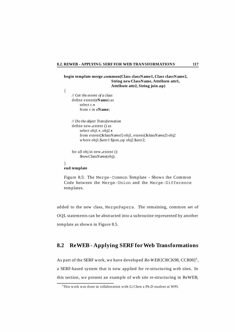
8.2. REWEB - APPLYING SERF FOR WEB TRANSFORMATIONS 117
begin template merge common(Class className1, Class className2,String newClassName, Attribute attr1,Attribute attr2, String join op)
// Get the extent of a classdefine extent(cName) as
select c.from c in cName;
// Do the object Transformationdefine new extent () as
select obj1., obj2.from extent($className1) obj1, extent($className2) obj2where obj1.$attr1 $join op obj2.$attr2;
for all obj in new extent ():$newClassName(obj);
end template
Figure 8.5: The Merge-Common Template - Shows the CommonCode between the Merge-Union and the Merge-Differencetemplates.
added to the new class, MergePapers. The remaining, common set of
OQL statements can be abstracted into a subroutine represented by another
template as shown in Figure 8.5.
8.2 ReWEB - Applying SERF for Web Transformations
As part of the SERF work, we have developed Re-WEB [CRCK98, CCR00]1,
a SERF-based system that is now applied for re-structuring web sites. In
this section, we present an example of web site re-structuring in ReWEB,
1This work was done in collaboration with Li Chen a Ph.D student at WPI.
8.2. REWEB - APPLYING SERF FOR WEB TRANSFORMATIONS 118
while most of the details can be found in [CCR00]. All displayed web pages
have been generated automatically by our Re-Web system.
First, assume the web administrator designs the web site structure of
a university’s computer science department. The index Home page pro-
vides three categories of information: Faculty members, Courses and Class-
Rooms, each of which has a link referring to its respective list. The Fac-
ultyList index page, under the Faculty sub-directory relative to the Home
page, lists all the faculty members of this department. Each faculty has a
link to a separate page named by the name of the faculty (for example, Elke
could be the name for her homepage), the personal information, as well
as a link to each course she teaches. Each Course page (that the department
provides) has Faculty links to all the instructors who are offering the course.
With this design of homepages within the department’s web site, the web
administrator basically captures this web semantics by designing the origi-
nal OODB schema as depicted in Figure 8.6. The desired web pages can be
generated accordingly (see the lower part of Figure 8.6).
In Figure 8.6, we assume there are objects that populate the database
already. Assume there is a Course object with courseNum “CS561”, two
faculty members are offering this course, one of them is Elke A. Runden-
steiner, whose personal information is included in a Faculty object. The
course offered by her is held in Fuller Lab 320 every Thursday night from
5:30 to 8:20 pm. The classroom location information is encapsulated in a
ClassRoom object. Thus there exists a bi-directional link between the Fac-
ulty object and the Course object, modeling a (zero to multiple) relationship.
Also there is a one-way relationship from the Course object to the ClassRoom

8.2. REWEB - APPLYING SERF FOR WEB TRANSFORMATIONS 119
Faculty
namephonerankteaches
Course
courseNumtime locationtaughtBy teaches
taughtBy
Course Class
<?xml version="1.0" ?><course xmlns="http://..."> <courseNum>CS561-AdvancedDB</courseNum>
<time>Th 5:30-8:20pm</time> <location xlink:href="../ClassRoom/CS561Loc" /> <taughtedBy xlink:href="../Faculty/Elke.xml"/> <taughtedBy xlink:href="../Faculty/Nabil.xml"/></course></xml>
ClassRoom
roomNumbuildingcampus
location
<?xml version="1.0" ?><faulty xmlns="http://..."> <name>Elke A. Rundensteiner</name>
<phone>831-xxxx</time> <rank>Associate Professor</rank> <course xlink:href="../Course/CS561.xml"/></faculty></xml>
<?xml version="1.0" ?><classroom xmlns="http://.."> <roomNum>320</roomNum> <building>Fuller</building> <campus>Worcester</campus></classroom></xml>
CS561.xml Elke.xmlCS561Loc.xml
Faculty ClassClassRoom Class
Figure 8.6: The ODMG Data Model and Corresponding XML Files for theOriginal Web Site.
object. Each of these three objects has an associated type in the OODB and
the relationships among them follow the OODB schema design.
In the underlying database, all objects of each class are maintained in
the class extent and all classes are registered by the schema dictionary. Thus
by scanning the schema dictionary, a set of XML files are generated by the
Re-Web system. Each of them corresponds to one object from the OODB.
We show some of the generated XML files in Figure 8.6. They are CS561.xml
under the new created subdirectory of Course, Elke.xml under the subdirec-
tory of Faculty and CS561Loc.xml under the subdirectory of ClassRoom. The
XLinks within the XML files capture the relationships between the objects
and simulate the navigation mechanism.
Lastly, based on these XML files, the corresponding home pages are
then generated using the LotusXSL processor [IBM98] provided by IBM
(see Figure 8.7). On the top of each page, there is a navigation bar indi-
cating the categories of home pages. Each category has an index page that

8.2. REWEB - APPLYING SERF FOR WEB TRANSFORMATIONS 120
contains the list of pages that falls into this category. For example, by click-
ing on the Faculty bar, a Faculty List index page is requested containing all
links to the faculty members.
Figure 8.7: The Generated Example Home Pages of Original Web Site
However, this web site schema may not meet the user’s requirements
and the user may instead desire a web view of the same data but with in-
formation in a more compact format. For example, by checking a faculty’s
home page, the user would like to be able to know about not only the per-
sonal information of this faculty, but also all the courses she is teaching as
well as the location of that course within the same page. Thus the web
site needs to be re-structured. The supporting database schema should be
as depicted in the left part of Figure 8.9. After performing the desired
view transformation using the chain nesting transformation depicted in
Figure 8.8 with the help of the SERF subsystem, the underlying database
is re-structured to correctly reflect the desired structure of the web site.
Again, using the WebGen subsystem, the restructured database schema
and its transformed objects are dumped out and represented in XML for-
mat (as shown at the right part of Figure 8.9). The screen-dump of a result-
ing example homepage is shown in Figure 8.10. The previous home page

8.2. REWEB - APPLYING SERF FOR WEB TRANSFORMATIONS 121
begin template nested-convert-to-literal ( Class inliningClassName, Attribute flattenAttrName, Integer nestLevel)
// inline the next level complex attribute into the specified inlineClass. inline ($inliningClassName, $flattenAttrName)
// decide for a class which of its attibutes is complex and to be flattened. define findAttrToFlatten (className) as: select a from MetaAttribute a, MetaClass c where a.classDefinedIn = className and a.attrType = c.name and nestLevel != 0
// starting at the inliningClass all complex attributes are flattened. for attr in findAttrToFlatten ($inliningClassName): nested-convert-to-literal($inliningClassName, attr, $nestLevel-1);end template
Figure 8.8: Nested Inline Template by Re-using Basic Inline Template.
<?xml version="1.0" ?><faulty xmlns="http://..."> <name>Elke A. Rundensteiner</name>
<phone>831-xxxx</time> <rank>Associate Professor</rank> <course> <courseNum>CS561-Advanced DB</courseNum> <time></time> <location> <roomNum>320</roomNum> <building>Fuller Lab</building> <campus>Worcester</campus> </location> </course></faculty></xml>
FacultyWithCourseIno
namephonerankteaches
courseNumtime location
roomNumbuildingcampus
acultyWithCourseIno Class AllInfoInElke.xml
Figure 8.9: The ODMG Data Modeland Corresponding XML Files forDesired Web Site
Figure 8.10: The Generated ExampleHome Pages of Desired Web Site
for the faculty named “Elke” has been transformed and now directly em-
beds all the information collected along the chain from itself to its Course
links and from there to their respective Classroom links.
The power of Re-WEB lies in its capabilities to do complex transforma-
8.3. SUMMARY 122
tions, i.e., those defined in the template library or user-defined transforma-
tions. The example presented above is one example that shows the ease
with which web pages can be re-structured using Re-WEB. The above ex-
ample however, requires that a link or a relationship between the two web
pages (or classes) must exist for its successful execution. However, a user
may wish to combine information from two disjoint web pages (no link)
and present it in one web page.
Figure 8.3 can be used to combine two disjoint classes and produce a
view that represents a union of the two classes. Figure 8.4 shows a tem-
plate which can combine two disjoint classes and produces a view that rep-
resents a difference of the properties of the two classes. This view can now
be generated by WebGen to produce a composite web page between two
otherwise disjoint web pages.
8.3 Summary
In order to validate the basic concepts of SERF, we have presented in this
chapter two case studies. The first highlights the ability to express different
semantics for the same operation using the SERF templates. The second
case study shows the utility of the SERF systems as a web site re-structuring
tool.

123
Chapter 9
Related Work
9.1 Specifying Schema Change
Simple and Complex Schema Evolution. Schema evolution is a problem
that is faced by long-lived data. The goal of schema evolution research is
to allow schema evolution mechanisms to change not only the schema but
also the underlying objects to have them conform to the modified schema.
One key issue in schema evolution is understanding the different ways of
changing a schema. The first taxonomy of primitive schema evolution op-
erations was defined by Banerjee et al. [BKKK87]. They defined consis-
tency and correctness of these primitives in the context of the Orion system.
Most systems today such as Itasca [Inc93], GemStone [BMO+89], Object-
Store [Obj93], and O2 [Tec94] provide similar evolution support for their
underlying object model.
In recent years, the advent of more advanced applications has led to
the need for support of complex schema evolution operations. [SHT+77,

9.1. SPECIFYING SCHEMA CHANGE 124
FFHI72, Bre96, Ler00, Cla92] have investigated the issue of more complex
operations. Much of the initial work [SHT+77, FFHI72] focused on con-
verting and re-structuring data from flat files to a database which often
required complex conversions. Shu et al. [SHT+77] proposed complex op-
erations such as SLICE to flatten a hierarchical structure, GRAFT to merge
two trees into one larger tree and SELECT to select trees based on some con-
dition. More recently, [Ler00] has introduced compound type changes in a
software environment, i.e., focusing only on the type changes and not the
changes to the object instances associated with the modified type. The pro-
posed compound type changes included Inline, Encapsulate, Merge, Move,
Duplicate, Reverse Link and Link Addition.
Breche [Bre96] proposed a similar list of complex evolution operations
for O2, i.e., which considered schema as well as object changes. Breche
shows that these advanced primitives can be formulated by composing the
basic primitives that are provided by the O2 system, and has shown the
consistency of these advanced primitives. User-customized object migra-
tion functions in the (C-like) programming language of O2 can however
be provided. A SERF template is similar to these complex operations pro-
posed by Breche [Bre96] in the O2 framework. However, while they al-
low users flexibility for the data transformations (migration functions), the
same flexibility is not available to the users at the schema level. Moreover,
this set of primitives, now more complex, is not extensible, i.e., a user can-
not add their own schema transformations. In summary, previous research
in database schema evolution provides the users with a fixed set of schema
evolution operations [FFM+95, BKKK87]. Adding extensibility to schema

9.1. SPECIFYING SCHEMA CHANGE 125
evolution is the focus of our effort.
Work similar to ours has been done in the context of database transfor-
mation. The schemas involved can be expressed in a variety of different
database models and can be implemented using different DBMSs. Shu et
al. [SHL75] introduced a new data translation language, CONVERT, for
translating between source items and target items. Their work was how-
ever primarily focused on hierarchically structured data and their set of
operations is also fixed. More recently, Davidson et al. define a new lan-
guage (WOL) [DK97] for specifying such database transformations. In our
work, we do not propose a new language. To the contrary, we combine a
standard database query language and schema evolution services into one
framework and strive to provide a consistent yet extensible environment
for doing both the schema and the data transformations.
A key requirement of SERF is access to the system dictionary via OQL.
For this, we expect the system dictionary (schema repository) of an OODB
to be fully ODMG-compliant. If a given OODB is not ODMG compliant,
then all SERF templates require modifications to utilize the specific nota-
tions of the proprietary schema repository of the OODB. This modification
of SERF templates can be eliminated if the query language used in SERF
is modified such that it allows uniform access of data and meta-data. One
such query language SchemaSQL has been proposed by Lakshmanan et al.
[LSS96]. SchemaSQL is an extension of SQL that allows for manipulation
of data and meta-data in relational multi-database systems. This has the
advantage of offering inter-operability for meta-data management in rela-
tional systems and is not bound to the low level implementation of the sys-
9.1. SPECIFYING SCHEMA CHANGE 126
tem dictionary. We are currently looking at extending OQL to allow similar
uniform data and meta-data access and thus provide transparency of the
low-level implementation [SCR00]. XSQL [KKS92] is a another example of
a query language that provides some of the features of SchemaSQL in an
object-oriented context.
Evolution of Persistent Languages and Object Databases. Persistent lan-
guages have made transparent the lines between a programming language
and a data store. However, persistent objects must also face their evolution.
In [RW98], Ridegeway et al. explore the evolution of classes in JSPIN. Here
they store class binaries in the database and evolution looks at binary com-
patibility and at evolving it. However, their implementation currently only
supports replacement of one binary with another. PJama, another persis-
tent language, also supports evolution [Dmi98]. They present an approach
that modifies the byte-code and verifies its authenticity before making it
persistent. One of their contributions is the incremental generation of the
byte-code depending on the schema evolution method.
Miscellaneous. Peters and Ozsu [PO95] have introduced an axiomatic
model that can be used to formalize and compare schema evolution mod-
ules of OODBs. They develop a formal basis for schema evolution research,
and we use their notation and model to represent the concepts presented
in this paper.

9.2. OPTIMIZATION OF SCHEMA EVOLUTION 127
9.2 Optimization of Schema Evolution
Research in schema evolution has also studied the issue of when and how
to modify the database objects to address such concerns as efficiency, avail-
ability, and impact on existing code. Research on this issue has focused on
providing mechanisms to make data and the system itself more available
during the schema evolution process, in particular deferred and immedi-
ate propagation strategies [FMZ94b, FMZ94a]. Such optimization strate-
gies are orthogonal to the issue of expressiveness and extensibility of the
schema evolution support and in principle either of these propagation strate-
gies could be implemented for our framework. In [FMZ94b, FMZ94a], a de-
ferred execution strategy is proposed for the O2 database system that main-
tains a history of schema evolution operations for a class and migrates ob-
jects only when actually accessed by the user. This allows not only for high
database availability but also amortizes the cost of the object transforma-
tions with that of a query lookup. However, no optimizations are applied
to this sequence of schema evolution operation(s) and the performance of
this deferred mechanism deteriorates as the set of queried objects grows
larger. Our approach [CNR00], while primarily optimizing the immediate
update mode, also complements the deferred mechanism by offering time
savings as the queried set of objects and the number of schema evolution
operations to be applied on it grows larger.

9.4. CONSISTENCY MANAGEMENT 128
9.3 Behavioral Consistency
Schema evolution can cause both structural as well as behavioral (code) in-
consistencies. Zicari et al. [DZ91], Navathe et al. [MNJ94] and others have
explored the effects of schema evolution on the methods defined for a class,
while others like Bergstein et al. [BH93] have looked at it from a software
perspective in terms of doing code transformations when schema evolu-
tion occurs. Ozsu et al. [OPS+95] have developed TIGUKAT, an Objectbase
for modeling the uniform semantics of behaviors on objects and have ex-
plored behavioral consistency for TIGUKAT. All of these above mentioned
works focus on the correctness of an individual schema evolution opera-
tion, and thus are a pre-requisite for our work. None of them addresses,
however, the problem of optimizing the sequence of one or even several
schema evolution operations as done by our work.
9.4 Consistency Management
Consistency management is often done at runtime and is normally handled
by transaction roll-backs. Work has been done towards providing behav-
ioral consistency, i.e., the consistency of class methods under evolving en-
vironments [DZ91, MNJ94]. While there are similarities in that their algo-
rithms are also detecting broken references, such approaches are also hard-
coded. In SERF, we push these constraints/invariants to a higher level thus
making them easy to update and also allowing for pre-execution verifica-
tion checks.

9.5. EXTENSIBLE SYSTEMS 129
Other approaches for consistency management in ODBs utilize pro-
gramming language support [VD91, AH90] such as assertions and excep-
tion handling mechanisms in languages like C++, Java and Ada. Relational
database systems (RDBMS) offer some additional support in the form of
triggers but provide only roll-back semantics, i.e., if a constraint is not sat-
isfied at the end of a transaction, then the entire transaction is rolled back
[EN96]. Active database systems [BCVG86, LLPS91, BK90] provide event-
condition-action (ECA) rules as a mechanism for detecting the occurrence
of some event and responding to it by some action.
Research has also been done in consistency management for software
process languages. Tarr et al. [TC98] have developed a consistency man-
agement system which allows for the specification of consistency condi-
tions and the degree of inconsistency tolerable by the user. Much of the
work in literature concentrates on detecting consistency violations and on
the specification of consistency constraints. We now try to utilize theorem
provers as a preventive measure to ensure that consistency violations do
not occur.
9.5 Extensible Systems
Hursch et al. [HS96] have proposed a framework that captures the depen-
dency between different components in a schema and code. When a change
occurs this dependency framework is used to formulate propagation pat-
terns to maintain behavioral consistency. They use propagation patterns
as a mechanism for maintaining programs. We propose here a similar ap-

9.5. EXTENSIBLE SYSTEMS 130
proach. However, we utilize a declarative approach for specifying the con-
straints embedded within schema evolution primitive code. We utilize the
notion of Contracts [Mey92] as first proposed by B. Meyer to specify the
constraints in a declarative fashion. Formal verification [GSW95, ORS92,
Bla98, GM93] techniques or more informal verification algorithms can be
utilized to verify the contracts.

131
Part III
Sangam - Managing Change in
Heterogeneous Databases


133
Chapter 10
Overview
Specifying and executing change on a source database is only one part
of the equation for change management. Typically, a database will have
many views, i.e., information that is derived from the source information.
A change in the source may result in changes or perhaps even in the invali-
dation of the view. Views and maintenance of views with respect to source
changes has been a lively topic in database research [ZGMHW95, GB95].
Much of the work in this area has been based on the assumption that both
the source and the view are defined within the confines of the same data
model, and often within the same database. Today this world is fast chang-
ing. Today many application engineers struggle to not only publish their
relational, object or ASCII file data on the Web but to also integrate infor-
mation from diverse sources. That is views are no longer in the same data
model as the source. Systems must therefore now address the issue of prop-
agation of change, where in, the derived information is not in the same data
model as the source.

CHAPTER 10. OVERVIEW 134
Current research addresses this problem by developing apriori algo-
rithms [TIHW01] that rely on the underlying translation algorithm between
the two data models. These apriori algorithms are tightly coupled to the
apriori algorithms used to derive the view from the source. We find that
because of this tight coupling, the apriori maintenance algorithms fall short
whenever there is a change in the translation technique between the same
two data models or if the maintenance algorithm is to be applied views
and sources in different data models. To meet the needs of maintaining
such across data model views, we consider current technology inadequate.
ITEM(id VARCHAR(10) NOTNULL, featured VARCHAR(100),location VARCHAR(200), mailBoxID VARCHAR(10),lastName VARCHAR(200), firstName VARCHAR(200))
MAIL(from VARCHAR(50), to VARCHAR(50),date VARCHAR(8), mailBoxID INTEGERCONSTRAINT fk id FOREIGN KEY (mailBoxID)REFERENCES ITEM(mailBoxID))
Figure 10.1: An Example Relational Schema.
To illustrate this problem, consider the fragment of the XMark bench-
mark DTD [SWK+01] shown in Figure 10.2 that is mapped to a relational
schema and data (Figure 10.1) via the basic inlining method [STZ+99]. The
basic inlining method inlines as many descendants of an element as pos-
sible into a single relation [STZ+99]. Consider now that the DTD (Fig-
ure 10.2) is modified and a new subelement reserve is added to the item
element. Figure 10.3 depicts the modified DTD. To ensure consistency of
the relational storage, this change should be propagated to the relational
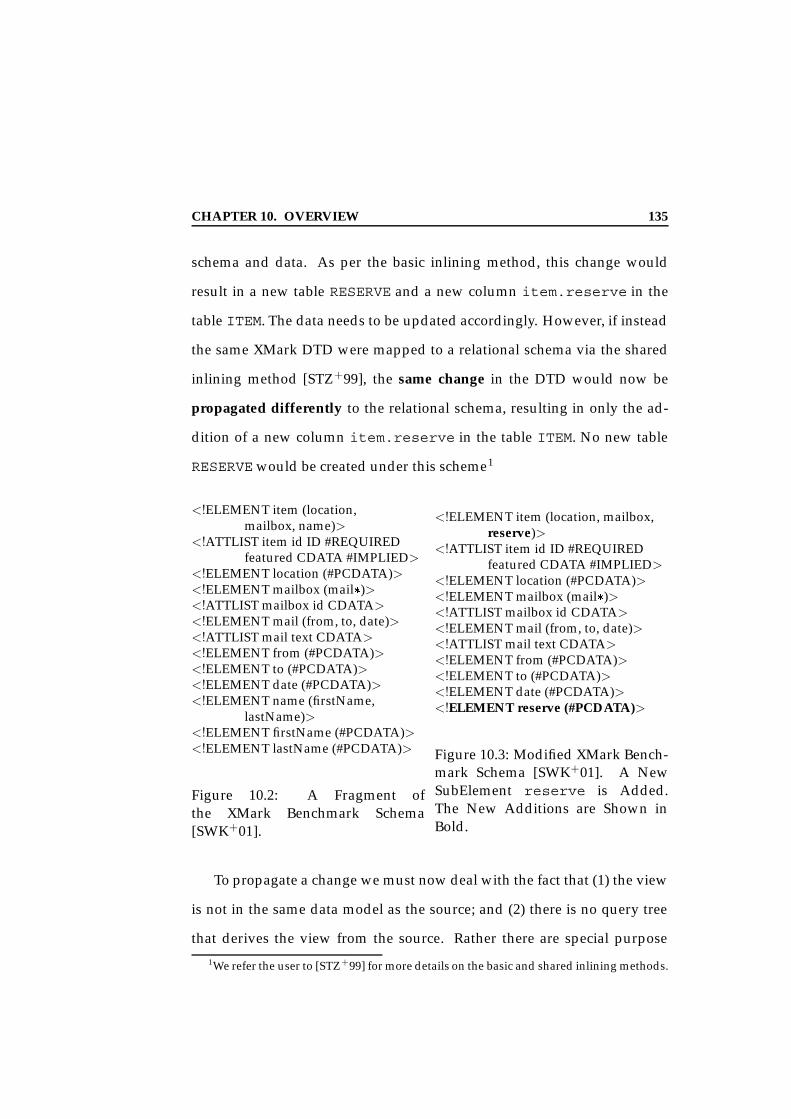
CHAPTER 10. OVERVIEW 135
schema and data. As per the basic inlining method, this change would
result in a new table RESERVE and a new column item.reserve in the
table ITEM. The data needs to be updated accordingly. However, if instead
the same XMark DTD were mapped to a relational schema via the shared
inlining method [STZ+99], the same change in the DTD would now be
propagated differently to the relational schema, resulting in only the ad-
dition of a new column item.reserve in the table ITEM. No new table
RESERVE would be created under this scheme1
<!ELEMENT item (location,mailbox, name)>
<!ATTLIST item id ID #REQUIREDfeatured CDATA #IMPLIED>
<!ELEMENT location (#PCDATA)><!ELEMENT mailbox (mail)><!ATTLIST mailbox id CDATA><!ELEMENT mail (from, to, date)><!ATTLIST mail text CDATA><!ELEMENT from (#PCDATA)><!ELEMENT to (#PCDATA)><!ELEMENT date (#PCDATA)><!ELEMENT name (firstName,
lastName)><!ELEMENT firstName (#PCDATA)><!ELEMENT lastName (#PCDATA)>
Figure 10.2: A Fragment ofthe XMark Benchmark Schema[SWK+01].
<!ELEMENT item (location, mailbox,reserve)>
<!ATTLIST item id ID #REQUIREDfeatured CDATA #IMPLIED>
<!ELEMENT location (#PCDATA)><!ELEMENT mailbox (mail)><!ATTLIST mailbox id CDATA><!ELEMENT mail (from, to, date)><!ATTLIST mail text CDATA><!ELEMENT from (#PCDATA)><!ELEMENT to (#PCDATA)><!ELEMENT date (#PCDATA)><!ELEMENT reserve (#PCDATA)>
Figure 10.3: Modified XMark Bench-mark Schema [SWK+01]. A NewSubElement reserve is Added.The New Additions are Shown inBold.
To propagate a change we must now deal with the fact that (1) the view
is not in the same data model as the source; and (2) there is no query tree
that derives the view from the source. Rather there are special purpose1We refer the user to [STZ+99] for more details on the basic and shared inlining methods.
CHAPTER 10. OVERVIEW 136
transformations which are most often in the form of a hard-coded module,
requiring different propagation algorithm for each change primitive, each
transformation, each pair of source and view (target) data models.
We address this problem of across data model maintenance using a two-
step approach. We first define a middle-layer integration framework and
as part of that a generic mapping language - the cross algebra, that can
define views such that there is no restriction that forces the view and the
source data models to be the same. Based on this algebra, we define update
propagation algorithms that enable the propagation of schema and data
changes from the source data model to the target data model.
Roadmap. Chapter 11 describes the graph model (Sangam graph) that we
use as our basic data model. Chapter 12 describes the cross algebra and the
different techniques of composing them into cross algebra graphs. Chap-
ter 13 describes the working implementation of the Sangam system and
presents the experimental validation of the same. In Chapter 14 we present
the set of change operations that can be applied on a Sangam graph, and
show how local changes in the relational or XML model can be mapped
into these. Chapter 15 describes our incremental update propagation al-
gorithm that can propagate these graph changes through the cross algebra
graphs. Chapter 16 presents our experimental results and Chapter 17 gives
an overview of the related work.
137
Chapter 11
Data Model
A key component of any middle-layer framework is the data model. The
choice of this common data model is crucial as the effectiveness of the mid-
dle layer is tightly coupled to the expressive power of the middle-layer
data model. A common data model must therefore be (1) be expressive
enough to structurally represent schemas from a variety of different data
models such as the relational, XML or object models; and (2) be able to
express a common subset of constraints, such as the order constraints in
XML, participation constraints (relational and XML), and other referential
constraints such as key and foreign key constraints. While we looked at
existing off-the-shelf data models we found that they did not adequately
support the requirements for a common data model. For example, while
the XML model satisfies the expressiveness property, it does not provide
adequate support for key and foreign key constraints 1. Similarly, the rela-
1The XML Schema specification given in May 2001 does provide support for keys andkeyrefs. However, the work in this dissertation was already under-way and towards com-pletion at that point.

11.1. SANGAM GRAPH MODEL 138
tional and the object model do not support order constraints.
In our work, we thus chose to develop a common data model - Sangam
graph model. The Sangam graph model is based on the common denomina-
tor of the existing data models - a graph, and can represent a subset of the
common constraints present in existing data models. We base our model
on the schema intension graphs (SIGs) from Miller et al. [MIR93]. The main
design emphasis of the SIGs is to measure the information capacity (the in-
tension [MIR93]) between different schemas of the same data model. While
the SIGs are used to model schemas within the same data model, namely
the relational model, we have found the SIGs to be sufficient to now also
represent schemas from other data models such as the XML model. We
term this simplified SIG the Sangam Graph Model (SGM).
11.1 Sangam Graph Model
The Sangam Graph Model M = (N , E) definesN a set of node types and E a
set of edge types. We categorize the node typesN of SGM as either complex
(2) or atomic ( ); and the edge types E as either containment (!) or property
(). A containment edge is an edge between two complex nodes, while a
property edge exists between a complex node and an atomic node. As the
discussion here focuses on complex nodes and containment edges, we use
the terms node and edge to imply these.
Sangam graph. The SGM allows us to model Sangam graphs. A Sang-
am graph G = (N , E , λ) is a directed graph where each node n 2 N is

11.1. SANGAM GRAPH MODEL 139
either complex or atomic, i.e.,τ : n ! N ; and each edge e 2 E is either a
containment or a property edge, i.e.,τ ’:e ! E ; and λ is a possibly infinite
set of labels.
Types. Each complex node n 2N represents a user-defined type, while each
atomic node represents a literal type such as a String or an integer. We denote
the set of user-defined types by Γ. Each node n is assigned a label l 2 λ,
i.e., τ”:n!l. Any node with only outgoing property edges is termed a
leaf.
NodeObjects. Each node n has associated with it a set of objects, termed
nodeObjects. Each nodeObject o 2 I (n) is a pair <id, v> where id is a glob-
ally unique identifier and v is its data value. We term this set of nodeOb-
jects the extent of the node n and denote this by I (n).
Relationships. The model permits the specification of binary relation-
ships between nodes, represented by directed edges between two nodes.
Each edge e 2 E is a labeled, directed edge between two nodes of N , with
label l 2 λ. An edge denoted as e:<n1, n2> indicates that e is an edge
from node n1 to node n2. Each edge is annotated with a set of properties
ζ , possibly empty. The set of annotations includes a local order, denoted by
ρ. This gives the relative local ordering for all outgoing edges from a given
node n in the Sangam graph. For example, given nodes n1, n2, n3, and
n4, if e1:<n1, n2>, e2:<n1, n3>, e3:<n2, n4> are three edges, then local or-
der defines the position of the edge e1 with respect to all other children2 of2We say that node nj is a child of node ni, if there exists an outgoing edge from ni to nj .

11.1. SANGAM GRAPH MODEL 140
node n1. In this example, ρ(e1) = 1 and ρ(e2)= 2. The local order of an
edge e is specified as an integer, and the local order of sibling edges is
continuous and differs by 1.
The quantifier annotation, denoted by Ω, associated with an edge e:<n1,
n2> specifies the subjectivity and injectivity of the binary relationship e
between the nodes n1 and n2. A quantifier is given as a pair of integers
[min:max], with 0 min max < 1 where min specifies the minimum
and max the maximum occurrences of nodeObjects of a node n2 for a given
nodeObject of node n1 associated via the binary relationship (edge) e.
EdgeObjects. Each edgee:<n1, n2> has associated with it a set of edgeOb-
jects. This set of edgeObjects is called the extent of the edge e and is denoted
by R (e). Each edgeObject oe 2 R is a triple <id,o1,o2> where id is a
system-generated identifier, nodeObject o1 2 I (n1) and nodeObject o2
2 I (n2). We denote the edgeObject using the edge notation, i.e., oe:<o1,
o2>. The edgeObject oe denotes that nodeObject o1 2 I (n1) is related
to nodeObject o2 2 I (n2). The set R may contain zero to multiple edges
between the same two nodes.
Based on the above, we define a valid Sangam graph as follows.
Definition 6 (Valid Sangam graph ) A Sangam graph G =(N, E, λ) is valid
if for all nodes n 2 N, τ (n) 2 N , and for all edges e 2 E , τ ’ (e) 2 E , and the
constraints (represented by the set of annotations ζ on an edge e) hold true by the
extent of the edge e, R(e).

11.2. CONVERTING APPLICATION SCHEMAS AND DATA TOSANGAM GRAPHS 141
11.2 Converting Application Schemas and Data to
Sangam graphs
A pre-requisite of our approach to achieve integration, is the ability to rep-
resent application schemas of different data models as Sangam graphs .
The nodes in a Sangam graph represent the constructs of the underlying
data model and the edges represent the relationships between the different
constructs. Annotations on the edges capture the various constraints that
may exist in the local data model. In this section we show how an XML
schema can be translated into a Sangam graph and the XML documents
corresponding to the XML schema can be placed as sets of objects (the ex-
tents) for the nodes and edges of the Sangam graph. We also show how the
same can be done for relational schemas and data.
11.2.1 XML and Sangam graphs
Loading the XML Schema/DTD. The loadXMLSchema algorithm shown
in Figures 11.1 and 11.2 is a two-pass algorithm that loads a given XML
schema (or DTD) into a Sangam graph representation. Figure 11.1 gives
the first pass while Figure 11.2 gives the second pass of the algorithm. In
the first pass a Sangam node is created for every XML entity, Element or
Attribute. The Sangam graph node is created by the method insertNode 3,
which takes as parameters: (1) the label of the node - this is the name of
the element or attribute; (2) the parent of the node - this is a Sangam graph
node and represents the DTD for an element node and an element for an3This operation is defined in Chapter 14

11.2. CONVERTING APPLICATION SCHEMAS AND DATA TOSANGAM GRAPHS 142
attribute node; (3) the edge label - the label for the binary relationship be-
tween the two nodes; (4) the quantifier - this is the quantifier annotation
for the edge; and (5) order - the order annotation for the edge. If the par-
ent node is specified as null, then the binary relationship, quantifier, and
order must also be set to null. In general, an edge from the node that rep-
resents an element to the node representing an attribute denotes the binary
relationship between the element and the attribute.
In the second pass, we load the content (definition) of elements. The
relationship between two elements, given by the nesting of the elements,
is denoted by a directed edge from the node p that represents the parent
element to the node n that represents the child element. In XML, the def-
inition of the child element is not inlined into the parent element. Rather
the definition of the child element is a separate entity that can then be used
by other parent elements. To model this in Sangam graphs, we introduce
the notion of a backpointer edge. The backpointer edge is a containment edge
that links a child node to its definition node. Thus, for every child node n
a backpointer edge is added to its defining node m, where the node m repre-
sents the definition of the child element and is created during the first pass.
This also enables us to handle recursion effectively in the Sangam graph.
An XML group is represented by a Sangam graph node and has an edge
from the node representing the parent element to the child node represent-
ing the group. If there are multiple children nested in a parent element,
the order of the children (be it a group or an element) is denoted by the
order annotation on the edges from the parent node to the child. Similarly,
the quantifier specifications “” - child can occur zero or more times, “+” -

11.2. CONVERTING APPLICATION SCHEMAS AND DATA TOSANGAM GRAPHS 143
function loadXMLSchema (XMLDTD xmlS)
DTDParser parser new DTDParser (xmlS , true )DTD dtd parser.parse// Create SAG Node for DTDSAGNode root createSAGNode(xmlS , NULL)// First Pass: Import the Root Elements and its AttributesEnumeration elemHash dtd.elementsint Eorder 1while (elem.hasMoreElements())
DTDElement e (DTDElement)elem.nextElement()// Create Sangam Node for ElementSAGNode elemNode createSAGNode(e.getName(), root, “elementEdge”,
1, Eorder)Enumeration attrs e.attributesint Aorder 1
// Traverse all Attributeswhile (attrs.hasMoreElements())
DTDAttribute a (DTDAttribute)attrs.nextElement()// Create Sangam Node for AttributeSAGNode attNode createSAGNode(a.getName(), elemNode,
“attributeEdge”, 1, Aorder)Aorder++
Eorder++
// Second Pass: Load the content of the XML Elements(subelements, groups)Enumeration elem dtd.elementswhile (elem.hasMoreElements())
DTDElement e (DTDElement)elem.nextElement()importContent(e,root)
return root
Figure 11.1: The LoadXML Algorithm to Translate an XML DTD into aSangam graph.

11.2. CONVERTING APPLICATION SCHEMAS AND DATA TOSANGAM GRAPHS 144
child can occur one or more times, ”?” - child can occur zero or one times,
and if none is specified then the child can occur exactly once, are translated
into quantifier annotations on the edge from the parent to the child. The
quantifier annotations are [0:n] for , [1:n] for +, [0:1] for ?, and [1:1]
otherwise. Currently, we cannot represent a group with a choice “|” in the
Sangam graph. Figure 11.2 represents the second pass of the algorithm. The
actual code for this can be downloaded from [Boo94].
Example 1 Figure 11.3 shows the Sangam graph for the XMark benchmark schema
of Figure 10.2. Here, each element and attribute is represented by a node. The
edges between nodes, for example, the edge e1 between the node labeled item and
location represents the binary relationship between the item element and its
sub-element location. The edge e1 has an order annotation of 1. The quanti-
fier annotation [1:1] on edge e1 denotes a functional edge, i.e., that there must be
exactly one value of location that can participate in a binary relationship with
one value of item. Similarly, the edge e2 between the nodes with labels item
and id represents the binary relationship between the XML element item and
its attribute id. The order annotation for this edge is 4. The order for attributes
is not part of the XML model but is assigned as part of the Sangam graph. The
information is discarded when converting the Sangam graph to an XML DTD or
to another data model that does not keep track of order. The quantifier annotation
[1:1] specifies a functional edge, i.e., there can only be one attribute id value per
element item value.

11.2. CONVERTING APPLICATION SCHEMAS AND DATA TOSANGAM GRAPHS 145
function importContent (DTDElement elem, SAGNode parent) // Check content of the Element
DTDITEM item elem.content()if item.getType() == (EMPTY jj PCDATA)
// returnelse
// Get quantifier and orderQuantifier quantifier item.getQuantifier ()int order item.getOrder ()if (item.getType()) == GROUP
// Create group node - assign a default NameSAGNode gseNode
createSAGNode(“gName”, parent, “groupEdge”,quantifier, order)
elseif (item.getType()) == ELEMENT
// Create subelement nodeSAGNode gseNode
createSAGNode(item.getName(), parent,“SubElementEdge”, quantifier, order)
// Get all the items of a subelement or groupEnumeration items = item.getItemsVec()for all it in items do:
importContent(it,gseNode)
Figure 11.2: The LoadXML Algorithm to Translate an XML DTD into aSangam graph - The Second Pass.
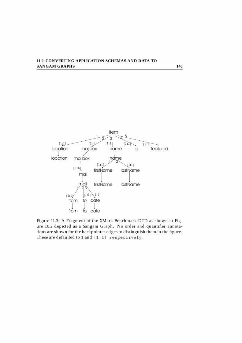
11.2. CONVERTING APPLICATION SCHEMAS AND DATA TOSANGAM GRAPHS 146
Figure 11.3: A Fragment of the XMark Benchmark DTD as shown in Fig-ure 10.2 depicted as a Sangam Graph. No order and quantifier annota-tions are shown for the backpointer edges to distinguish them in the figure.These are defaulted to 1 and [1:1] respectively.

11.2. CONVERTING APPLICATION SCHEMAS AND DATA TOSANGAM GRAPHS 147
Loading the XML Data. While it is not necessary to materialize the Sang-
am graph, i.e., load the XML documents as objects of the Sangam graph
nodes and edges, we present here for completeness one algorithm for ex-
tracting the XML documents and representing them as the extent of Sang-
am graph nodes and edges. The XML document is loaded into a DOM tree
structure4. We traverse the DOM tree, root down, in a depth first manner.
For each XML element, we first locate the matching Sangam graph node.
The matching Sangam graph node is determined based on (1) name equal-
ity, i.e., the element tag and the label of the Sangam graph node must be
the same; and (2) the context, i.e., the element tags of all the elements in the
path from the root to the element must be the same as the labels of all the
Sangam graph nodes from the root to the matching node. This is similar to
the Xpath identification. For every attribute the Sangam graph node match
is done similarly but is much simpler as the context for an attribute is given
directly by the parent element. Once a Sangam graph node match (called
matching node) is found, then data in the XML document is translated as
follows:
1. if it is an XML attribute, then a new object oi is created with a unique
identifier and the attribute value is translated as the value of the ob-
ject.
2. if it is a non-PCDATA element or a group, an object oi is created with
a unique identifier and a null value.
3. if it is a PCDATA element, then a new object oi is created with a4We use Java’s XML parsers to do this.

11.2. CONVERTING APPLICATION SCHEMAS AND DATA TOSANGAM GRAPHS 148
unique identifier. The PCDATA value is stored as the value of the
object.
In each of the above three cases, a new edgeObject oe is created for the
edge between the parent Sangam graph node (representing the element)
and the current Sangam graph node 5. The object is oe represented as oe:
<op, oi>, where object op is the parent object6, and oi is the child object.
Example 2 Figure 11.4 shows an XML document conforming to the XMark DTD
given in Figure 10.2. The XML fragment given in Figure 11.4 is mapped as the
extent of the Sangam graph given in Figure 11.3 as follows: after the match for the
element item is found, a new object o1 is created with an identifier and a null
value. The XML attribute id with value 1 is translated into an object o2 for the
node labeled id. The value of this object is set to 1. A new object is also created
with the object pair oe:<o1,o2> and is inserted into the extent of the edge between
the nodes item and id. Similarly, the element location with the PCDATA
value of ‘Paris’ results in a new object o3 whose value is set to ‘Paris’. A
new object created with the value pair <o1, o3> is inserted into the extent of the
edge between the nodes with labels item and location. The element mailbox
is a non-PCDATA element. Hence an object o4 is created with a null value and
is inserted into the extent of the node with label mailbox. The rest of the XML
document is translated similarly. Figure 11.5 displays the Sangam graph with
corresponding extents for each node and edge.
5The edge itself is established during the load XML Schema process.6Since we are doing a depth-first traversal, we always have a handle on the current
parent object.

11.2. CONVERTING APPLICATION SCHEMAS AND DATA TOSANGAM GRAPHS 149
<?xml version=”1.0” standalone=”yes”? >
<item id=“1”, featured = ’no’><location> Paris < /location><mailbox> <mail mail=’All set’>
<from> Peter </from><to> Pat </to><date> Sept 23, 2001 < /date>< /mail>
< /mailbox><name><firstName>Peter< /firstName>
<lastName> Unger < /lastName>< /name>
< /item>
Figure 11.4: A Fragment of the XMark Benchmark Document Conformingto the XMark Benchmark Schema in Figure 10.2.
Generating XML from a Sangam graph. The process of loading the XML
DTD into a Sangam graph is preserving, i.e., the same XML DTD can now
be generated from the Sangam graph by an inverse algorithm. Complex
nodes in the Sangam graph represent the elements and the attributes. We
further classify that a complex node with only atomic children nodes can
be regarded as an XML attribute. All other nodes in the Sangam graph
represent elements. Using this distinction of nodes, the XML DTD and
document fragments can now be built by doing an in-order traversal of the
Sangam graph starting at the root, and reversing the translation process
done during the load time.

11.2. CONVERTING APPLICATION SCHEMAS AND DATA TOSANGAM GRAPHS 150
Figure 11.5: The Extent of the Sangam graph in Figure 11.3 based onthe XML Document given in Figure 11.4. Part (a) depicts the extent.Here we show the extent of each node, and the extent of edge e:<item,location>. Part (b) presents just the object structure.
11.2.2 Relational Schemas and Sangam graphs
Loading the Relational Schema. Similar to the loading of an XML DTD,
we first look at the algorithm for representing a relational schema as a Sang-
am graph. This algorithm is similar to the one given for the XML DTD in
Figure 11.1. We give the main intuition based on an example. Figure 11.6
presents a relational schema with two tables and a foreign key constraint
between the two tables. Each schema construct is first translated into a
node in the Sangam graph. The schema constructs include a table and

11.2. CONVERTING APPLICATION SCHEMAS AND DATA TOSANGAM GRAPHS 151
a column. The domain type of each column is represented by an atomic
node in the Sangam graph. For example, considering the relational schema
in Figure 11.6 the table ITEM is represented by a node. Each of its columns,
location, mailBoxId, id, featured, etc. is represented by complex
nodes in the Sangam graph. The label of each node is the table or the col-
umn name respectively. The domain of a column is represented by atomic
nodes. These are omitted from the figure to maintain its clarity.
ITEM(id VARCHAR(10) NOTNULL, featured VARCHAR(100),location VARCHAR(200), mailBoxID VARCHAR(10),lastName VARCHAR(200), firstName VARCHAR(200))
MAIL(from VARCHAR(50), to VARCHAR(50),date VARCHAR(8), mailBoxID INTEGERCONSTRAINT fk id FOREIGN KEY (mailBoxID)REFERENCES ITEM(mailBoxID))
Figure 11.6: An Example Relational Schema.
All relationships, including the parent-child relationship between a ta-
ble and its column, are represented by an edge from, for example, the
node that represents the ITEM table to the node that represents the id col-
umn. As the relational model does not have order, the order annotation for
each edge is defaulted to a serially increasing number during the schema
load time. The quantifier annotation for an edge is decided based on the
NOTNULL and the UNIQUE constraints on a column. If a column is set to
NOTNULL, then the minimum quantifier on the edge between the parent
(table node) and the node (column node) is set to 1; else it is set to 0. If a
column is UNIQUE, then the maximum quantifier for the edge is set to 1;

11.2. CONVERTING APPLICATION SCHEMAS AND DATA TOSANGAM GRAPHS 152
else it is set to1 to denote multiple occurrences.
Foreign key relationships between two tables are modeled by an edge
between the node that represents the primary key column and the node
that represents the foreign key column. The label of the foreign key edge is
set to the name of the foreign key. In the example schema of Figure 11.6 this
is fk id. The order annotation is defaulted during the load, and the quan-
tifier annotation is set to [0:n] to denote that one object of the primary key
node may refer to zero or more objects of the foreign key node. Figure 11.7
represents the relational schema of Figure 11.6 as a Sangam graph.
Figure 11.7: Relational Schema of Figure 11.6 depicted as a Sangam graph.
Loading the Relational Data. Again, the Sangam graph representation
of the relational schema can be materialized if needed. Figure 11.1 depicts
the relational tables ITEM and MAIL and their respective data. Similar to
loading of XML documents, the relational data is read column-wise, i.e., all
values of a particular column in a table. An object o with a unique object-
identifier is generated for each row of the table. This object o is placed in
the extent of the node that represents a table. For example, for the first row
in the ITEM table, a new object is created and placed in the extent of the
node m with label ITEM. Within the row, for each column a new object oc is

11.2. CONVERTING APPLICATION SCHEMAS AND DATA TOSANGAM GRAPHS 153
created. The value of the object oc is set to the column’s value. The object
oc is then placed into the extent of the node n that represents the column.
A new edge object oe is also created such that it now contains the pair
<o, oc>. This edge object is placed in the extent of the edge e between the
nodes m and n. Values for other columns in the same row and consequently
for the other rows are translated in a similar manner. Figure 11.5 gives the
extent of the SAG obtained by translating the tables in Table 11.1.
id featured location mailBoxID lastName firstName1 no Paris 1 Unger Peter
from to date mailBoxIDPeter Pat Sept 23, 2001 1
Table 11.1: Example Relational Tables ITEM and MAIL are Represented asExtent of the SAG as shown in Figure 11.5.
Generating Relational Schema and Data from a Sangam graph The
loading process of the relational schema and data can be reversed to now
translate the Sangam graph into a relational schema and the correspond-
ing set of relational data. Similar to the generation of XML, for relational
schema generation we distinguish Sangam graph nodes that represent re-
lations versus those that represent attributes. An attribute is a complex
node with only outgoing property edges. All other nodes represent rela-
tions. An edge between two nodes representing relations is translated to
a foreign key construct. In addition to the reversing process to convert the
Sangam graph into a relational schema, we also need to resolve two issues.
One, a Sangam graph can handle set-valued attributes whereas the rela-
11.3. SUMMARY 154
tional model cannot. We deal with this by building a separate relation and
linking to the parent relation using a foreign key. The second is recursion.
Recursion in a Sangam graph occurs when a cycle is formed when travers-
ing a node with a backpointer edge. To handle recursion, each node with a
backpointer edge that forms a cycle is translated to a new separate relation.
Other than these distinctions, the process of translating a Sangam graph to
a relational schema and data is a simple reverse of the loading algorithm.
11.3 Summary
In this chapter, we have described the data model utilized in our mid-
dle layer called the Sangam graph model. We have given algorithms to
translate local application schemas in the XML and relational models into
Sangam graphs, as well as algorithms to transform the corresponding data
into Sangam graph extents.
The Sangam graph model can express the structure of schemas in a va-
riety of data models such as the XML, relational, extended relational and
object models. The Sangam graph constructs can express the common set
of constraints in the relational and the XML model such as the key con-
straints, foreign key constraints, order and participation constraints. How-
ever, they cannot currently express constraints such as the functional de-
pendency constraints.
One disadvantage of building a new data model is the lack of tools that
exist for our unified data model - Sangam. This set of tools includes: a
query language, a transformation language, parsers, design tools etc. These
11.3. SUMMARY 155
tools come for ”free” if the unified data model is a high-level, commercial
model such as the relational model or the XML model. However, as we
will show in the next Chapter, there are many significant advantages for
defining a low-level transformation language, and we believe that these
compensate for some of the disadvantage.

11.3. SUMMARY 156

157
Chapter 12
Cross Algebra
The purpose of our proposed cross algebra is to enable the transforma-
tion of an application schema and its associated data in one data model to
an application schema and data in another model. To accomplish this the
cross algebra operators transform a given input Sangam graph to an out-
put Sangam graph. The cross algebra allows linear transformations [GY98]
of the Sangam graph, i.e., nodes and edges of the input Sangam graph are
mapped via the cross algebra operators to nodes or edges in the output
Sangam graph. The linear transformations of a graph are the fundamental
transformations, on the basis of which other more complex transformations
can be defined [GY98]. The cross algebra operators include the cross op-
erator denoted by for the addition of a node to the output Sangam graph
; the connect operator denoted by for the addition of a binary rela-
tionship between two nodes (an edge) in the output Sangam graph ; the
subdivide denoted by < for splitting a binary relationship (an edge) in
the input Sangam graph to a pair of binary relations (two edges) in the

12.1. CROSS ALGEBRA OPERATORS 158
output Sangam graph ; and the smooth operator denoted by =, for con-
verting two binary relations (two edges) in the input Sangam graph to one
binary relation in the output Sangam graph. Deletion of nodes or edges
can simply be accomplished by not mapping a given construct in the input
Sangam graph to the output Sangam graph.
In this section, we detail the functionality of cross algebra operators.
For each cross algebra operator we describe the transformation of the input
Sangam graph (nodes, edges and set of objects associated with the nodes
or edges) to the output Sangam graph (nodes, edges and set of objects re-
spectively) that is accomplished by it; and preconditions, if any. We show
how these algebra operators can be composed together to represent a al-
gebra expression (Section 12.2). In Section 12.3.1, we present a binding of
these operators to physical algebra operators and show how these can be
evaluated. In the last section, Section 12.4 we give a complete example to
show how basic inlining and shared inlining [STZ+99] techniques can be
represented by these algebra operators, and hence show how XML can be
transformed into relational schemas and data by a cross algebra expression.
12.1 Cross Algebra Operators
12.1.1 The Cross Operator
The cross algebra operator corresponds to a node creation operation in
the output Sangam graph. It takes as input a node n in the input Sangam
graph and produces as output a node n’ in the output Sangam graph. The
cross operator is a total mapping, i.e., the objects in the extent of n given
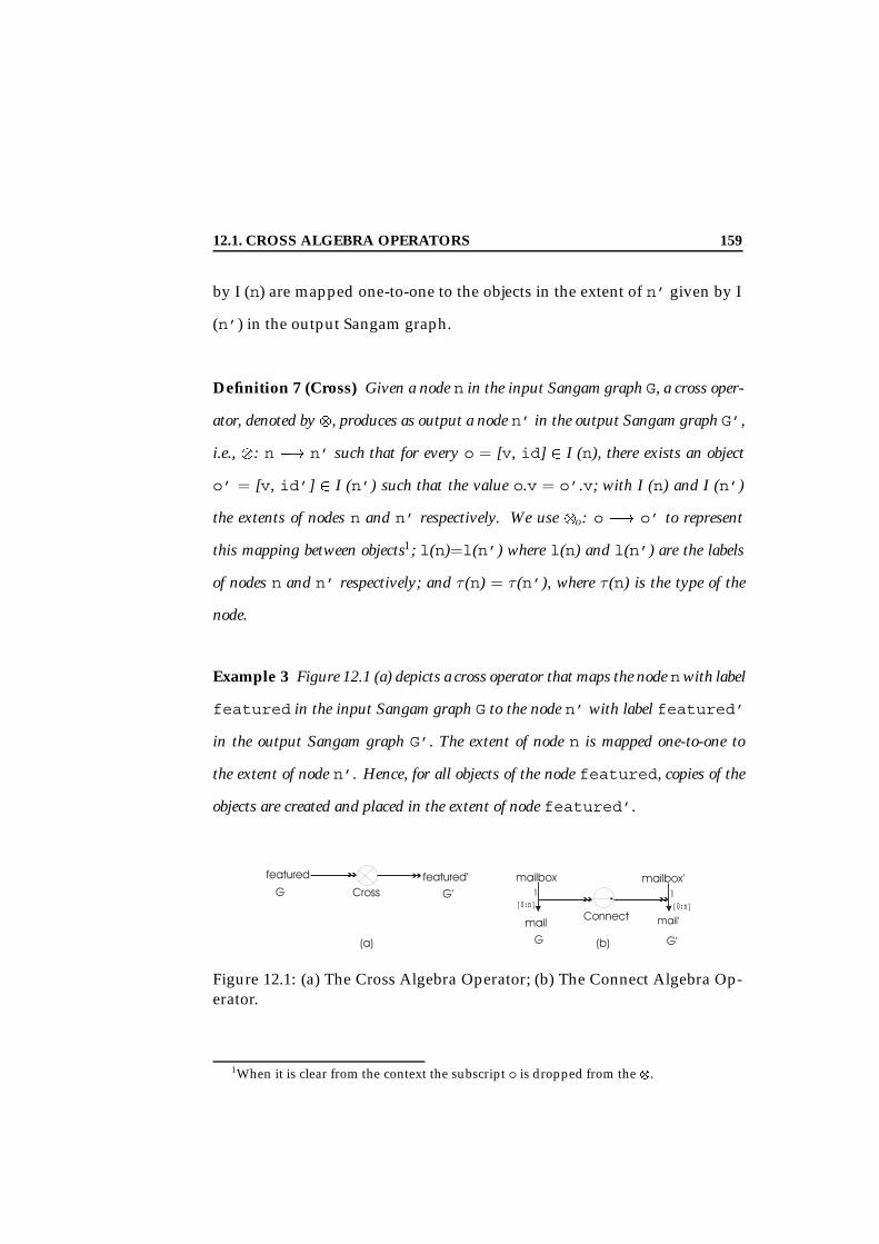
12.1. CROSS ALGEBRA OPERATORS 159
by I (n) are mapped one-to-one to the objects in the extent of n’ given by I
(n’) in the output Sangam graph.
Definition 7 (Cross) Given a node n in the input Sangam graph G, a cross oper-
ator, denoted by , produces as output a node n’ in the output Sangam graph G’,
i.e., : n ! n’ such that for every o = [v, id] 2 I (n), there exists an object
o’ = [v, id’] 2 I (n’) such that the value o.v = o’.v; with I (n) and I (n’)
the extents of nodes n and n’ respectively. We use o: o ! o’ to represent
this mapping between objects1; l(n)=l(n’) where l(n) and l(n’) are the labels
of nodes n and n’ respectively; and τ (n) = τ (n’), where τ (n) is the type of the
node.
Example 3 Figure 12.1 (a) depicts a cross operator that maps the node nwith label
featured in the input Sangam graph G to the node n’ with label featured’
in the output Sangam graph G’. The extent of node n is mapped one-to-one to
the extent of node n’. Hence, for all objects of the node featured, copies of the
objects are created and placed in the extent of node featured’.
Figure 12.1: (a) The Cross Algebra Operator; (b) The Connect Algebra Op-erator.
1When it is clear from the context the subscript o is dropped from the .
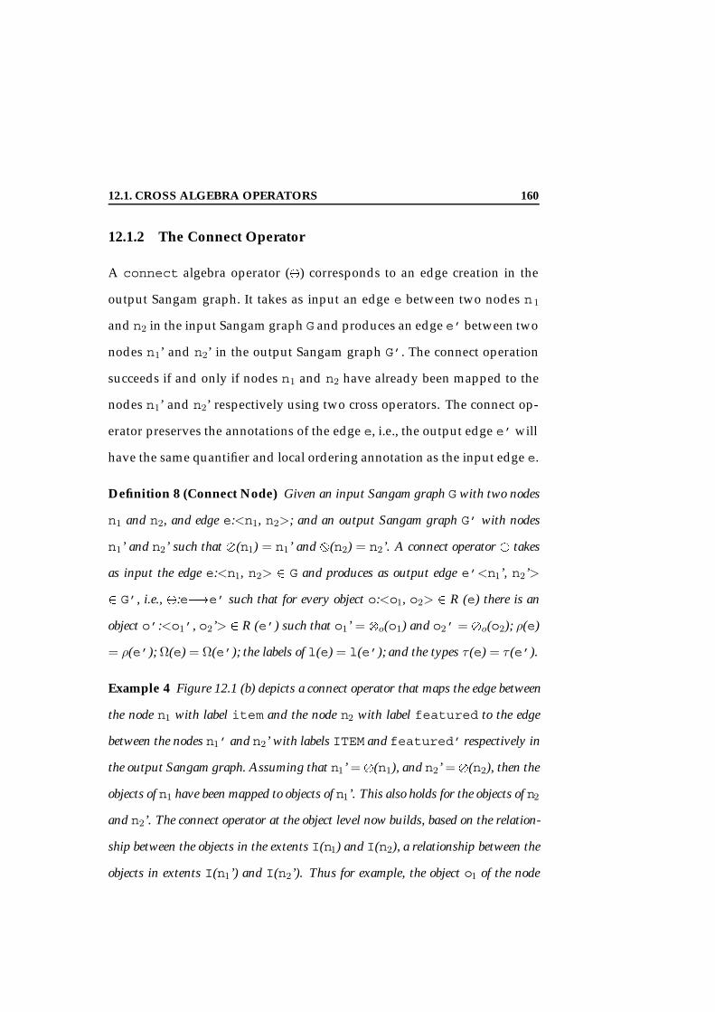
12.1. CROSS ALGEBRA OPERATORS 160
12.1.2 The Connect Operator
A connect algebra operator () corresponds to an edge creation in the
output Sangam graph. It takes as input an edge e between two nodes n 1
and n2 in the input Sangam graph G and produces an edge e’ between two
nodes n1’ and n2’ in the output Sangam graph G’. The connect operation
succeeds if and only if nodes n1 and n2 have already been mapped to the
nodes n1’ and n2’ respectively using two cross operators. The connect op-
erator preserves the annotations of the edge e, i.e., the output edge e’ will
have the same quantifier and local ordering annotation as the input edge e.
Definition 8 (Connect Node) Given an input Sangam graph G with two nodes
n1 and n2, and edge e:<n1, n2>; and an output Sangam graph G’ with nodes
n1’ and n2’ such that (n1) = n1’ and (n2) = n2’. A connect operator takes
as input the edge e:<n1, n2> 2 G and produces as output edge e’<n1’, n2’>
2 G’, i.e., :e!e’ such that for every object o:<o1, o2> 2 R (e) there is an
object o’:<o1’, o2’> 2 R (e’) such that o1’ = o(o1) and o2’ = o(o2); ρ(e)
= ρ(e’); Ω(e) = Ω(e’); the labels of l(e) = l(e’); and the types τ (e) = τ (e’).
Example 4 Figure 12.1 (b) depicts a connect operator that maps the edge between
the node n1 with label item and the node n2 with label featured to the edge
between the nodes n1’ and n2’ with labels ITEM and featured’ respectively in
the output Sangam graph. Assuming that n1’ =(n1), and n2’ =(n2), then the
objects of n1 have been mapped to objects of n1’. This also holds for the objects of n2
and n2’. The connect operator at the object level now builds, based on the relation-
ship between the objects in the extents I(n1) and I(n2), a relationship between the
objects in extents I(n1’) and I(n2’). Thus for example, the object o1 of the node

12.1. CROSS ALGEBRA OPERATORS 161
item is in relation with the object o2 with value true of the node featured.
The connect operator will now build a relationship between the object o11 of the
node ITEM and the object o22 with value true of the node featured’. This
assumes that o11 = o(o1) and o22 = o(o2).
12.1.3 The Smooth Operator
Let a Sangam graph G have three nodes n1, n2, and n3, and two binary
relations represented by edges e1:< n1, n2 > and e2:< n2, n3 > as shown
in Figure 12.2. The smooth (=) operator replaces the binary relations rep-
resented by edges e1 and e2 in the Sangam graph G with a new binary
relation represented by edge e’:< n01, n03 > in the output Sangam graph G’.
The smooth operator is successful only if(n1) = n1’ and(n3) = n3’. The
local order annotation on the edge e’ is set to the local order annotation of the
edge e1, i.e., ρ(e’) = ρ(e1). However, the edge e’ has a larger information
capacity as it is a result of combining the capacities of relations represented
by edges e1 and e2. Hence, the quantifier annotation of the edge e’ is given
as: Ωmin(e’) = Ωmin(e1) Ωmin(e2); and Ωmax(e’) = Ωmax(e1) Ωmax(e2).
The smooth operator produces a surjective edge e’ if both e1 and e2 are
surjective, or an injective edge e’ if both e1 and e2 are injective.
Definition 9 (Smooth Operator) Let G be an input Sangam graph with three
nodes n1, n2, and n3, and edges e1:< n1, n2 > and e2:< n2, n3 >. Let G’ be an
output Sangam graph with nodes n1’ and n3’ such that (n1) = n1’, and (n3)
= n3’. A smooth operator = maps the edges e1:<n1, n2> and e2:<n2, n3> 2
G to produce the edge e’:< n10, n30 > 2 G’ such that each pair of objects oe1:<

12.1. CROSS ALGEBRA OPERATORS 162
Figure 12.2: The Functionalityof the Smooth Operator. Figure 12.3: An Example of the Smooth
Operator.
o1, o2 > and oe2:< o2, o3 > in R (e1) and R (e2) respectively, are represented
by one edge object oe3:<o1’, o3’> 2 R (e’’) where o1’ = o(o1) and o3’ =
o(o3’); ρ(e’) = ρ(e1); and Ωmin(e’) = Ωmin(e1) Ωmin(e2); and Ωmax(e’)
= Ωmax(e1) Ωmax(e2); the labels of e’ and e1 are the same; and the types of e’
and e1 are the same, i.e., τ (e’) = τ (e1).
Example 5 Figure 12.3 depicts a smooth operator that maps the edges e1: <Per-
son, mailbox>, and e2: <mailbox, mail> to the edge e3’: <PERSON,
MAIL>. Edge object o1: <’Peter’,’Box1’>2 2R (e1) and object o2: <’Box1’
,’All Done’ > 2 R (e2) are mapped and a new object o3 is created such that
o3:<’Peter’, ’All Done’>. The object o3 2 R (e3’). The mapping of the
objects is done as explained for the connect operator.
12.1.4 The Subdivide Operator
A subdivide operator < performs the inverse operation of the smooth
operator. LetG be a Sangam graph with two nodesn1 and n3 and edgee’:<
n1, n3 > (Figure 12.4). The subdivide operator introduces a new node n2’
2We use values here instead of oids for clarity of the example.

12.1. CROSS ALGEBRA OPERATORS 163
into the output Sangam graph G’ such that the edge e’ in G is replaced by
two edges e1 and e2 in the output Sangam graph G’: one between nodes
n1’ and n2’ represented by edge e1; and the other between nodes n2’
and n3’ represented by e2. The subdivide operator is successful only
if (n1) = n1’ and (n3) = n3’. The local order annotation for the edge
e1:< n1, n2 > is the same as that for the edge e’, i.e., ρ(e1) = ρ(e’) as they
are incident from mapped nodes, i.e., (n1) = n1’. The edge e2 is the only
edge added for the node n2’ and thus has a local order annotation of 1, i.e.,
ρ(e2) = 1. During the subdivide operation, to preserve all the edges that
exist between the extents I(n1) and I(n3) of nodes n1 and n3 respectively,
the output edges e1 and e2 are assigned quantifier annotations as follows.
If Ωmin(e’) = 0, then the quantifier range for e1, Ω(e1) = [0 : 1], else Ω(e1) =
[1 : 1]. The quantifier of edge e2, Ω(e2) = Ω(e’). Thus the two edges e1 and
e2 model a surjective relationship if e’ models a surjective relationship.
Figure 12.4: The Functionalityof the Subdivide Node. Figure 12.5: An Example of the Subdi-
vide Node.
Definition 10 (Subdivide Operator) Let G be an input Sangam graph with
two nodes n1 and n3 and an edge e’. Let G’ be the output Sangam graph G’
with nodes n1’, n2’ and n3’ such that (n1) = n1’, and (n3) = n3’. A subdivide

12.1. CROSS ALGEBRA OPERATORS 164
operator < takes as input the edge e’:<n1, n3> 2 G, and produces as output one
node n2’ and two edges e1:<n1’, n2’> and e2:<n2’, n3’> 2 G’, such that (1)
each edge object oe1:<o1, o3> 2 R (e) is mapped to edge object o0e1:<o1’,on2>
2 R (e1), and edge object oe2’:<on2, o3’> 2 R (e2) where o1’ = o(o1), o3’
= o(o3), and on2 is a new node object that is created such that on2 2 I (n2’);
(2) Ωmin(e1) = 0, if Ωmin(e’) = 0, and Ωmin(e1) = 1 otherwise; Ωmax(e) = 1;
Ω(e2) = Ω(e’); ρ(e1) = ρ(e’) and ρ(e2) = 1; the labels of e1 and e2 are set to be
the same as the label of e’; the types of e1 and e2 are set to be the same as the type
of e’; the label of the new node n2’ is set to a system-defined label; and τ (n2’) =
τ (n1).
Example 6 Figure 12.5 depicts the inverse of the smooth operator example from
Figure 12.3. It divides the edge e3’:<PERSON, MAIL> into two edges namely,
e1:<Person, MailBox>, and e2:<MailBox, Mail>. Here an edge object
oe:<’Peter’, ’All Done’>, relates the object o13 2 I (PERSON) and the
object o3 2 I (MAIL) in the input Sangam graph. A new object o2’ is created and
inserted into the extent of the node MailBox. A new edge object oe1 is created
such that oe1:<o1’, o2’> with o1’ = o(o1). A new edge object oe2 is created
such that oe2:<o2’, o3’> with o3’ = o(o3). The edge object oe1 is inserted
into the extent R (e1) and the edge object ee2 is inserted into the extent R (e2).
Hence, all objects that were connected by one edge are now connected by a path of
two edges.
3This object represents the object with value Peter.

12.2. CROSS ALGEBRA TREES 165
12.1.5 Notation
We use the notation given in Table 12.1 to indicate the cross algebra oper-
ators. In general, opout(in) represents an algebra operator that operates on
input in, where in is either a node or an edge (or two edges for the smooth
operator) in a Sangam graph, and produces the output out which again is
either a node or an edge (or a node and two edges for the sub-divide op-
erator) in a Sangam graph. These are specified using the labels assigned to
the nodes or edges in a Sangam graph.
Notation Descriptionn0 (n) Cross operator with input n and output
n’e0 (e) Connect operator maps edge e:<n1, n2>
to edge e’:<n1’, n2’>=e0 (e1, e2) Smooth node maps edges e1:<n1,n2>
and e2:<n2,n3> to edge e’:<n1’,n3’>in the output
<e10,e20,n20(e) Subdivide node maps edgee:<n1,n3> to e1’:<n1’,n2’> ande2’:<n2’,n3’> in the output
Table 12.1: Notation Used for Cross Algebra Operators.
12.2 Cross Algebra Trees
In relational algebra, algebra operators are nested to form one algebra ex-
pression. These operators are combined together via derivation by applying
one operator(s) to the result of one or more operators. The relational al-
gebra has the advantage of operating within the relational model, i.e., its
12.2. CROSS ALGEBRA TREES 166
input and output are both relational. Moreover, each relational algebra op-
erator operates on complete relations, treating a relation as the basic unit for
input and output. Attributes of a relation for example can only be mapped
(or not mapped, in the case of projection) into attributes of the output rela-
tion (and only if the relation itself is mapped). In other words, the schema
of the output is implied by the semantics of the relational operators, i.e.,
each operator has a built-in template of the output schema. Similarly, XML
algebra operates on the granularity of an ordered collection of XML frag-
ments, where each fragment is a complex nested XML element and pro-
duces as output also an ordered collection of XML fragments [FFM+01a].
Cross algebra, however, operates at the granularity of individual nodes
and edges in a Sangam graph. A cross operator takes a node as input and
produces a node as output, whereas the connect, smooth and subdivide op-
erators operate on edge(s) in the Sangam graph and produce edge(s) as out-
put (possibly adding or removing nodes). However, the difference between
the cross algebra, and the relational and XML algebras, lies in the fact that a
node in a Sangam graph may represent data model specific constructs such
as an XML element, or a relational table, or an XML/relational attribute.
Correspondingly, an edge may, for example, represent the relationship be-
tween an XML element and its attribute, or a foreign key between two re-
lations. An algebra that goes crosses different data models must therefore
be flexible in order to accommodate the variance in the sizes of modeling
units of each individual data model. For example, the modeling unit for
the relational model is two-level deep, i.e. relations and their columns,
whereas for XML it is n-level deep and at times recursive thereby allowing

12.2. CROSS ALGEBRA TREES 167
nested element structures. As we cannot predict the right granularity to
accommodate all data models, we use the smallest granularity within the
Sangam graph as a modeling unit. This has the advantage of allowing the
mapping of constructs and relationships in one data model to constructs
and relationships in another data model. However, given this low-level of
granularity we now need additional mechanisms to express the mapping
of arbitrary complete units such as a relation or a complex nested element
from the input graph to the output graph. To enable this, we introduce a
new type of composition of cross algebra operators that allows several al-
gebra operators to collaborate and jointly operate on different parts of the
input Sangam graph, and together produce one (connected) Sangam graph.
We term this a context dependency composition. In this section, we give details
of the more traditional derivation composition of the cross algebra opera-
tors, the context dependency composition, and the combination of the two
compositions into one valid algebra expression.
12.2.1 Derivation Trees
Figure 12.6 gives an example of a derivation composition that transforms
the path in the Sangam graph shown in Figure 12.6 (a) to the edge in the
Sangam graph given in Figure 12.6 (c) by applying three smooth nodes =.
Let e1:<A,B>, e2:<B, C>, e3:<C, D> and e4:<D, E> be edges in the input
Sangam graph G. Operators op1e10(e1, e2) and op2e20(e3, e4) are applied
to the input edges e1 and e2, and e3 and e4 respectively to first produce
the intermediate edges e1’:<A’, C’> and e2’<C’, E’> as shown in Fig-
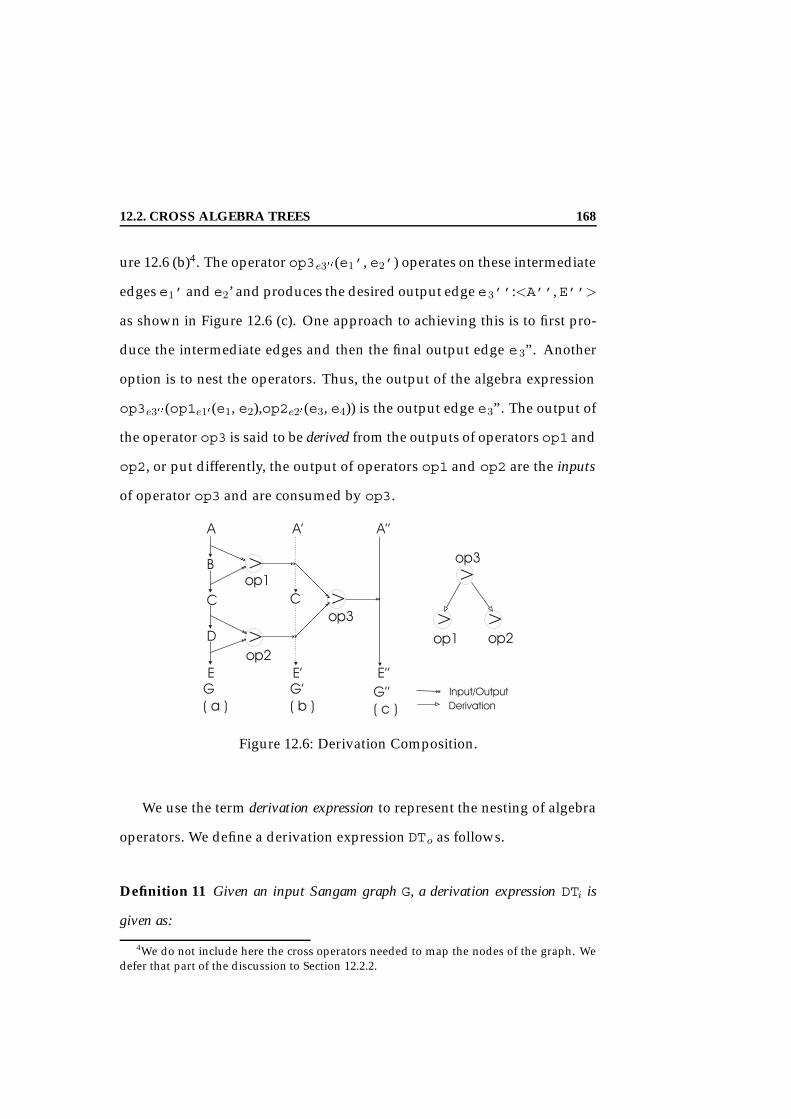
12.2. CROSS ALGEBRA TREES 168
ure 12.6 (b)4. The operator op3e300(e1’, e2’) operates on these intermediate
edgese1’ and e2’ and produces the desired output edge e3’’:<A’’,E’’>
as shown in Figure 12.6 (c). One approach to achieving this is to first pro-
duce the intermediate edges and then the final output edge e3”. Another
option is to nest the operators. Thus, the output of the algebra expression
op3e300(op1e10(e1, e2),op2e20(e3, e4)) is the output edge e3”. The output of
the operator op3 is said to be derived from the outputs of operators op1 and
op2, or put differently, the output of operators op1 and op2 are the inputs
of operator op3 and are consumed by op3.
Figure 12.6: Derivation Composition.
We use the term derivation expression to represent the nesting of algebra
operators. We define a derivation expression DTo as follows.
Definition 11 Given an input Sangam graph G, a derivation expression DTi is
given as:
4We do not include here the cross operators needed to map the nodes of the graph. Wedefer that part of the discussion to Section 12.2.2.

12.2. CROSS ALGEBRA TREES 169
DTo(outo)(ino) =
8>>>>>>>>>>>>>>>>>>>>>>>>>>>>>>>>>>>>><>>>>>>>>>>>>>>>>>>>>>>>>>>>>>>>>>>>>>:
opi(outi)(ini) for a single operation opi 2 ,
,=,< with opi semantics as
defined in Definitions 7, 8, 9 and
10
opi(outi)
(DTj(outj)(inj)) where opi 2 , , < and
DTj a derivation tree and ini =
outj
opi(outi)
((DTk(outk)(ink)),
(DTl(outl)(inl))) where opi 2 =, and DTk and
DTl are derivation trees and ini
= outk, outl
produces as output outo node and edge elements for an output Sangam graph G’,
such that outo is the output of the root operator opi and thus also of the complete
derivation tree DTo.
Here outo denotes the output of the derivation tree DTo, that is Sang-
am graph nodes or edges generated by DTo; and ino denotes the input,
i.e., Sangam graph nodes and/or edges, the derivation tree operates on.
The output of the derivation tree DTo is equal to the output outi, i.e., the
output produced by the top-most algebra operator op i of the derivation

12.2. CROSS ALGEBRA TREES 170
tree. When DTo is a derivation tree with more than one algebra operator,
then the output of the outermost op i is calculated by using as input the
outputs generated by its respective inner nested derivation trees DT j or
(DTk and DTl). Here the nested derivation trees generate the inputs of the
operator opi.
We use “(” and “)” pairs to denote nesting, i.e., derivation of opi from
the derivation tree DTj . We use the symbol “,” to separate input arguments
of an operator opi.
A derivation expression is graphically represented as a derivation tree.
Definition 12 Given a derivation expression DTo as defined in Definition 11, TD
= (No, Ed) is a derivation tree such that (1) each node ni 2 No represents a cross
algebra operator (, , =, <) in DTo; and (2) each edge ei 2 Ed represents the
nesting “(” and ”)” in DTo, as a derivation edge_ from the parent (outer nested)
operator opi to each of the children (inner nested) operators. If any child (inner
nested) operator itself is a derivation expression DTj , then a derivation edge_ ex-
ists from the parent (outer nested) operator opi to the root operator of the internal
derivation tree DTj .
Henceforth, we use the terms derivation expression and derivation tree
interchangeably and distinguish between them only when needed.
Consider the derivation tree in Figure 12.6. The expression for this tree
is given as:
DT1 = op3e300(op1e10(e1, e2), op2e20(e3, e4)) (12.1)

12.2. CROSS ALGEBRA TREES 171
Graphically, this is represented by two derivation edges from the parent
operator op3 to the children operators op1 and op2, given as op3_op1,
and op3_op2. Note that a derivation tree alone cannot be guaranteed
to produce a valid output. For example, op3 here produces an edge e3’’
without any end nodes. This edge alone is not a valid Sangam graph. In the
next few sections, we discuss how a derivation tree can be used to indeed
produce valid output.
Lemma 4 A derivation tree TD as defined in Definition 12 and given by the ex-
pression DTo(outo)(ino) is a rooted directed acyclic graph (DAG).
Proof: This can be proven by a simple proof by induction.
Base Case - Let DTo(outo)(ino) = opi(outi)(ini). As the DT is comprised of
one operator only, clearly it is acyclic and there is only one root.
Hypothesis - Let:
DTk(outk)(ink) = opk(outk)(DTj(outj)(inj)) (12.2)
such that DTk is a derivation tree with k operators. Let us assume that
DTk with k operators is acyclic, (i.e., that all edges (derivation edges) from
the root operator opk are in the same direction from the root to its children
(leaves of the tree)), and rooted.
Induction k k+1 - Let us assume that we have a derivation tree DTk with
k operators. We can now construct a derivation tree DTk+1 with k+1 oper-
ators in the following three ways:

12.2. CROSS ALGEBRA TREES 172
Case 1: Operator opk+1 is added as the new root of DTk. The resulting
derivation tree DTk+1 is a DAG.
Let opk+1 be the root operator of DTk+1 such that:
DTk+1(outk+1)(ink+1) = opk+1(outk+1)(DTk). (12.3)
Re-writing Equation 12.3 using Equation 12.2, we get:
DTk+1(outk+1)(ink+1) = opk+1(outk+1)(opk(outk)(DTj(outj)(inj))) (12.4)
That is, a single derivation edge exists from the root operator opk+1 to
its direct child operator opk (Definition 12). We know by our hypothesis
that a derivation tree DTk given as DTk = opk(outk)(DTj(outj)(inj)) (Equa-
tion 12.2) with k operators is acyclic, and all its edges are from the root opk
to its children. Since DTk+1 has k + 1 operators with a derivation edge
from the root opk+1 to opk, all the edges are in the same direction, i.e., from
the root to the children. Hence, DTk+1 is acyclic as well.
Case 2: Operator opk+1 is added as the new leaf of DTk. The resulting
derivation tree DTk+1 is a DAG.
Case 3: Replace existing subtree DTi with a new tree DTi+1 with i +
1 operators. We know that DTi+1 is a DAG, as i < k. Hence, the new
derivation tree DTk+1 is also a DAG. 2
12.2. CROSS ALGEBRA TREES 173
12.2.2 Context Dependency Trees
While a derivation tree may consume multiple edges and nodes as input,
it always produces exactly one edge or one node, or in the case of the sub-
divide root operator one node and two edges as defined above (Defini-
tion 11). It never produces an entire output Sangam graph. Nor can com-
plete output Sangam graphs be produced by individual operators that are
not nested. Consider the three cross algebra operatorsop1 (), op2 () and
op3 (=) that map the node A to A’, B to B’ and the edge e:<A, B> to edge
e’:<A’, B’> respectively. Without a mechanism to represent a grouping
of these operators, it is not possible to indicate (1) that the three operators
together work on the same input Sangam graph and produce one single
output Sangam graph G’ composed of two nodes A’ and B’, and an edge
e’:<A,B> as shown in Figure 12.7; (2) the operator op3 can be success-
fully evaluated only after the evaluation of op2 and op1; and (3) output of
op1 and op2 is used by op3 but not consumed by it.
To remedy this, we introduce a context dependency tree to express the
above semantics. A context dependency tree CT represents a rooted, hi-
erarchical grouping of cross algebra operators that together map an input
Sangam graph G to an output Sangam graph G’. Each operator op in the
context dependency tree CT operates on individual nodes or edges in the
input Sangam graph G and maps them to individual nodes or edges in the
same output Sangam graph G’.
Figure 12.7 denotes such a context dependency tree CT composed of
three cross algebra operators. Here, the algebra operators op1A0(A) and

12.2. CROSS ALGEBRA TREES 174
op2B0(B) are cross operators that map the nodes A and B in G to nodes A’
and B’ respectively in the output Sangam graph G’. The algebra operator
op3e0(e), a operator is the root of CT and maps the edge e:<A, B> be-
tween the nodes A and B in the input Sangam graph G to the edge e’:<A’,
B’> between the nodes A’ and B’ in the output Sangam graph G’. Here
the outputs of all operators op1, op2, and op3 together produce the output
Sangam graph G’.
Figure 12.7: Context Dependency Composition Example.
This grouping of algebra operators, called context dependency tree, is de-
noted by CTo and is defined as follows.
Definition 13 Given an input Sangam graph G, a context dependency tree CTo

12.2. CROSS ALGEBRA TREES 175
specified as:
CTo(outo)(ino) =
8>>>>>>>>>>>>>>>>>>>>>>>>>>>>>>>>>>>>>>>>><>>>>>>>>>>>>>>>>>>>>>>>>>>>>>>>>>>>>>>>>>:
opi(outi)(ini) for a single operation opi 2
, , =, <, and outo =
outi
opi(outi)(ini),
(CTk(outk)(ink))
[Æ (CTl(outl)(inl))]+)
where opi is the parent op-
erator of CTk and CTl de-
noting that opi must be ex-
ecuted after CTk and CTl.
opi uses outputs, inputs and
mapping of CTk and CTl
and outo = outjS
outkS
outl. The symbol []+ is part
of the grammar syntax and is
defined below.
operates on nodes ni and edges ei 2 G, and produces as output a Sangam graph G’
such that all nodes ni’ and/or edges ei’ produced as output by any of the individual
operators opi 2 CT are in G’.
Here ino denotes the input of the context dependency tree CT o, that is
Sangam graph nodes or edges of graph G. The expression outo denotes the
final output of the context dependency tree CTo. The output outo is the
union of the outputs of all operators that compose the context dependency

12.2. CROSS ALGEBRA TREES 176
tree. Thus, in Definition 13, outo = outiSoutk
Soutl, to denote that the
final output is the output of the operator opi and the context dependency
trees CTk and CTl.
In Definition 13 the symbol “+” is part of the BNF grammar syntax to
indicate that the expression contained in “[ ]” may occur one or more times.
Definition 14 Given a context dependency expression CTo as defined in Defini-
tion 13, TC = (No, Ec) is a context dependency tree such that (1) each node ni 2
No represents a cross algebra operator (, , =, <) in the expression CTo; and
(2) each edge ei 2 Ed is a context dependency edge! from the parent (left) oper-
ator to the child (right) operator, and represents the symbol “,” in the expression
CTo. The symbol “Æ” in the expression CTo is denoted by fact that the operators
(or trees) share a common parent (left) operator. No edges exist between the sibling
operators. If a parent (left) operator has more than one child, where the children
(right) operators are separated by Æ, then a context dependency edge exists from
the parent (left) to each of the children (right) operators. If a child (right) operator
is a context dependency tree, then the context dependency edge! exists from the
parent operator opi to the root operator opj of the context dependency tree.
Henceforth, we use the terms context dependency expression and con-
text dependency trees interchangeably and distinguish between them only
when necessary.
Thus, the expression for the context dependency tree in Figure 12.7 may
be given as:

12.2. CROSS ALGEBRA TREES 177
CTout(in) = op3e0(e), (op1A0(A) Æ op2B0(B)). (12.5)
Here the operator op3 is the root of the context tree, and op1 and op2
are the children operators. Here e:<A, B> and e’:<A’, B’>. The final
output out = e’SA’SB’ corresponds to the final output SAG G’.
The context dependency expression CTo is evaluated from right to left
and from inside out. That is all children operators are evaluated prior to
the evaluation of their parent operator. The order of evaluation between
the sibling operations is immaterial.
Beyond the order of evaluation, the context dependency relation be-
tween two operators op3!op1 (Figure 12.7) implies that the operator op3
uses the following three pieces of information in its calculation: (1) the in-
put of op1; (2) the output of op1; and (3) the mapping φ of op1 as estab-
lished by the type , , = and < of op1 given in Definitions 7, 8, 9, and
10.
Lemma 5 A context dependency tree TC as defined in Definition 14 and given by
the expression CTl(outl)(inl) (Definition 13) is a rooted, directed acyclic graph.
Proof: This can be proven by a simple proof by induction.
Base Case - Let CTo(outo)(ino) = opi(outi)(ini). As the CTo is comprised of
one operator only, clearly it is acyclic.
Hypothesis - Let:

12.2. CROSS ALGEBRA TREES 178
CTk(outk)(ink) = opk(outk)(ink), (CTj(outj)(inj)) (12.6)
be a context dependency tree such that CTk is a context dependency tree
with k operators. Let us assume that CTk with k operators is acyclic, and
all edges (context dependency edges) are in the same direction, i.e., from
the root opk to the children (leaves).
Induction -
Case 1: Operator opk+1 is added as the new root of CTk.
Given any CTk+1, by Definition 13 we have:
CTk+1(outk+1)(ink+1) = opk+1(outk+1)(ink+1), (CTk(outk)(ink)) (12.7)
Re-writing this expression using Equation 12.6 we have:
CTk+1(outk+1)(ink+1) = opk+1(outk+1)(ink+1), (opk(outk)(ink), (CTj(outj)(inj)))
(12.8)
That is a single context dependency edge exists from the parent (left)
operator opk+1 to the child operator opk. We know by our hypothesis
that a context dependency tree given as: CTk = (opk(outk), (CTj(outj)(inj)))
(Equation 12.6) is acyclic, and all its edges are from the parent opk to the

12.2. CROSS ALGEBRA TREES 179
children (leaves) operators. Since CTk+1 has k + 1 operators with a con-
text dependency edge from the parent opk+1 to opk, all edges are in the
same direction. Hence, CTk+1 is acyclic.
Case 2: Operator opk+1 is added as the new leaf of CTk.
Given any CTk+1, by Definition 13 we can have:
CTk+1(outk+1)(ink+1) = opk(outk)(ink), (CTj(outj)(inj) Æ opk+1(outk+1)(ink+1))
(12.9)
That is the operatoropk+1 is a child operator of opk, and a single context
dependency edge exists from the parent (left) operator opk to the child op-
erator opk+1 (Definition 14). We know by our hypothesis that a context de-
pendency tree given as: CTk = (opk(outk), (CTj(outj)(inj))) (Equation 12.6)
is acyclic, and all its edges are from the parent opk to the children (leaves)
operators. Since CTk+1 has k + 1 operators with a context dependency
edge from the parent opk to opk+1, all edges are in the same direction.
Hence, CTk+1 is acyclic.
Case 3: Some tree CTi is replaced by a new tree CTi+1. As i < k, we
know by our assumption that CTi+1 is a DAG. 2
12.2.3 Cross Algebra Graphs (CAG):
Combining Context Dependency and Derivation Trees
In general, an expression that translates an input Sangam graph G to an
output Sangam graph G’ corresponds to an ordered set of context depen-

12.2. CROSS ALGEBRA TREES 180
dency trees, derivation trees or a combination of context dependency and
derivation trees. We use the term cross algebra tree (CAT) to refer to the in-
dividual trees and the term cross algebra graph (CAG) to refer to the graph
representing this expression. Figure 12.8 gives an example of a cross alge-
bra graph (CAG) that translates a given input Sangam graph G to an output
Sangam graph G’. Here let e1:<A, B>, e2:<B, C>, e3:<C, D> and e4:<D,
E> represent edges in the input Sangam graph G. Let e’:<A’, E’> repre-
sent an edge in the output Sangam graph G’. The cross algebra tree CAT in
Figure 12.8 is given as:
CAT = CAT3 (12.10)
The output of the tree CAT3 is the final output of the CAT. The expres-
sion for CAT3 is given as follows:
CAT3 = DT1, (op1A0(A) Æ op3E0(E)) (12.11)
The output of CAT3 is produced by the evaluation of its expression,
namely, by the evaluation of the three inputs, namely the derivation tree
DT1, and the two cross algebra operators op1 and op3. Using the order of
evaluation for context dependency trees as specified in Section 12.2.2, the
operators op1 and op3 must be evaluated prior to the evaluation of DT1.
The evaluation of those two primitive operators op1 and op3 produces

12.2. CROSS ALGEBRA TREES 181
Figure 12.8: A Cross Algebra Tree.
the nodes A’ and E’ respectively. Given that op1 and op3 are in context
dependency relation with the root of DT1, the outputs of op1 and op3 now
become part of the final output of CAT3. The tree DT1 is given as:
DT1 = op6e0:<A0,E0>(CT1, CT2) (12.12)
The operator op6 represents the root of DT1, a derivation tree. The out-
put of this derivation tree (and hence of op6) is the edge e’ between the
nodes A’ and E’. This output is produced by the evaluation of the expres-
sion op6e0:<A0,E0>(CT1,CT2). Here the inputs for the operator op6 are the
edges in the input graph produced by the context dependency trees CT1

12.2. CROSS ALGEBRA TREES 182
and CT2 respectively. As per the definition of derivation (Definition 11),
the temporary outputs (the output Sangam graph) generated by the con-
text dependency trees CT1 and CT2 do not manifest themselves in the final
output of the derivation tree. The expression for CT1 is given as follows:
CT1 = op4eTemp1:<A0,C0>(e1 :< A, B >, e2 :< B, C >), (op1A0(A) Æ op2C0(C))
(12.13)
Observation 1 If there exists a derivation edge _ from an operator opi to the
root operator opj of a context dependency CTj, then the output Sangam graph G’
produced by the context dependency tree CTj serves as the input Sangam graph
for the operator opi. The operator opi directly consumes only one node or edge of
Sangam graph G’ (or two nodes and edges if opi = =) and produces a node or an
edge as output (or a node and two edges if opi= <) (Definition 11).
In the above example, op6 consumes the edge eTemp1 produced by
the context dependency tree CT1 as well as the edge eTemp2, the output
produced by CT2. The Sangam graph G’ is an intermediate Sangam graph
and is discarded, i.e, G’ and the edge eTemp1:<A’, C’> do not appear in
the final output of op6. Similar to CT1, the expression for CT2 is given as:
CT2 = op5eTemp2:<C0 ,E0>(e3 :< C, D >, e4 :< D, E >), (op2C0(C) Æ op3E0(E))
(12.14)

12.2. CROSS ALGEBRA TREES 183
To summarize the above example (Figure 12.8), the context dependency
trees CT1 and CT2 produce two intermediate Sangam graphs G’ and G’’
that smooth the edges e1 and e2 to produce edge eTemp1 and smooth
edges e3 and e4 to produce edge eTemp2 respectively. The operator op6
then gets its inputs from CT1 and CT2 and produces the edge e’:<A’,E’>.
The operator op6 also participates in the tree CAT3, the output of which is
the final Sangam graph G’’’ with nodes A’, E’ and the edge e’:<A’,
E’>. Thus, the CAT in Figure 12.8 operates on the input Sangam graph G
and produces as output the Sangam graph G’’’.
As shown by the example above, operators may participate in more
than one context dependency or derivation tree, i.e., they may appear mul-
tiple times in the CAT algebra expression. These shared operators are evalu-
ated only once during the evaluation of the complete CAT expression, and
hence contribute output once (versus multiple times) in the evaluation of
the CAT. We say that two operators are the same if they observe the follow-
ing conditions.
Definition 15 (Same Operators) Two operators opi and opj are identified as
being the same in one CAT, if they have the (1) same mapping type (cross, smooth,
etc.); (2) same input node or edge (from the same input Sangam graph G) as iden-
tified by its label and identifier; and (3) produce as output the same node or edge in
the same Sangam graph G’ based on its label and identifier5.
Definition 16 (Evaluation Semantics of Shared Operators) If two operators
opi and opj are the same as per Definition 15, then they are termed shared op-5Recall from Chapter 11 each node and edge in a Sangam graph has a unique identifier.

12.2. CROSS ALGEBRA TREES 184
erators. Each shared operator is evaluated once, and contributes directly6 at most
once to the final output graph G’ produced by the CAT.
Formally, we define a CAT expression as follows:
Definition 17 (CAT) A CAT is an expression that operates on one or more input
6Some other operator opk may derive from it. The output of operator opk may appearin the final output.

12.2. CROSS ALGEBRA TREES 185
Sangam graphs G and produces one or more output Sangam graph G’ such that:
CATo(outo)(ino) =
8>>>>>>>>>>>>>>>>>>>>>>>>>>>>>>>>>>>>>>>>>>>>>>>>>>>>>>>>>>>>>>>>>>>>>>><>>>>>>>>>>>>>>>>>>>>>>>>>>>>>>>>>>>>>>>>>>>>>>>>>>>>>>>>>>>>>>>>>>>>>>>:
DTi(outi)(ini) where DTi is as per Def-
inition 11
CTi(outi)(ini) where CTi is as per Def-
inition 13
(CATj(outj)(inj)) ,
((CATk(outk)(ink))) where CATj is parent of
CATk such that CATk
must be evaluated prior
to the evaluation of
CATj and outo = outjSoutyk.
opj(outj )
(CATk(outk)(ink)) where opj derives its in-
put inj from the output
outk produced by CATk,
and outo = outzj .
opj(outj )((CATk(outk)(ink)),
(CATl(outl)(inl))) where opj derives its in-
put inj from the outputs
outk and outl produced
by CATk and CATl re-
spectively, and outo =
outγj .

12.2. CROSS ALGEBRA TREES 186
y = A context dependency edge is added from the root op j of CATj to the
root opk of CATk.
z = A derivation edge is added from opj to opk, the root of CATk.
γ = A derivation edge is added from opj to opk and opl, the roots of CATk
and CATl respectively..
Definition 18 Given a CAT expression CATo as defined in Definition 17, a CAT
tree TCAT = (No, E) such that (1) each node ni 2 No represents a cross algebra
operator (, , =, <) in the expression CATo; and (2) each edge ei 2 Ed is either
a derivation edge_ or a context dependency edge! with semantics as defined in
Definitions 12 and 14 respectively.
Lemma 6 A CAT tree TCAT (Definition 18) given by the expression CATo (Defi-
nition 17) is a rooted, directed acyclic graph.
Proof.
A CAT as defined in Definition 17 can be either a context dependency
tree, a derivation tree or a composition of the two. We consider each case
individually. Definition 15 defines the criteria for designating operators as
shared operators. While at a practical level it is more efficient to physically
share the operators across different trees, for the purpose of the discussion
here, we assume that these shared (same) operators are physically distinct
operators. That is there exist multiple copies of the same operator in the
CAT7. In the forthcoming discussion we thus do not treat shared operators7Note that in the CAT expression, we do already represent shared operators by multiple
copies of the same operator.
12.2. CROSS ALGEBRA TREES 187
as a special case.
• CATout(in) = CTi(outi)(ini): We know by Lemma 5 that a context
dependency tree is acyclic.
• CATout(in)= DTi(outi)(ini): We know by Lemma 4 that a derivation
tree is acyclic.
• CATout(in)= CATj(outj)(inj), CAGk(outk)(ink): Let CAGj and
CAGk(outk) be any cross algebra trees such that they are acyclic. The
expressionCATj(outj)(inj), CAGk(outk)(ink) denotes that there exists
a context dependency edge from opj the root of CATj to opk the root
of CAGk, making CAGk a child of the root opj . As CAGj is acyclic with
all edges going from the root opk to the children, and CATk is similar,
it follows that after the addition of a context dependency edge from
opj to opk in the same direction, CATout is also acyclic.
• CATout(in) = opj(outj)(CATk(outk)(ink)): Let CATk be a cross al-
gebra tree that is acyclic. The expression opj(outj)(CATk(outk)(ink))
denotes that there exists a derivation edge from opj to opk, where
opk is the root of CATk. As CATk is acyclic with all edges going from
the root opk to the children, then it follows that after the addition of
a derivation edge from opj to opk, the edges are all still in the same
direction. Hence, CATout is also acyclic.
• CATout(in)= opj(outj)((CATk(outk)(ink),(CATl(outl)(inl))): Here
the operator opj is a binary operator with two inputs CATk and CATl.
The proof of this can given in a similar manner to the one above.

12.2. CROSS ALGEBRA TREES 188
Figure 12.9: Another Example of a Cross Algebra Graph.
2
Consider now an example CAG in Figure 12.9. Here the CAG operates
on input Sangam graph G and produces as output the Sangam graph G’.
The edges of G are e1:<A, B>, e2:<A, C>, e3:<B, D>, e4:<B, E> and
e5:<C, F>. Similarly for G’, the edges are e1’:<A’, B’>, e2’:<A’,
F’>, e3’:<B’, D’>, and e4’:<B’, E’>. The expression for this is given
by the following CAG:
CAG = (CT1 Æ CT2 Æ CT3 Æ CT4) (12.15)
where CT1 = op3(e10)(e1), (op1A0(A) Æ op2B0(B))
CT2 = op5(e20)(e2, e5), (op1A0(A) Æ op4F0(F))
12.2. CROSS ALGEBRA TREES 189
CT3 = op7(e30)(e3), (op2B0(B) Æ op6D0(D)) and
CT4 = op9(e40)(e4), (op2B0(B) Æ op8E0(E)).
Here note that the operators op2 and op1 are shared operators and
hence are used multiple times in individual context trees. However, as
per the evaluation semantics of shared operators (Definition 16), these op-
erators are only evaluated once during the evaluation of the CAG, and their
output only appears once in the output Sangam graph G’. Also note that
the output of context dependency trees CT1, CT2, CT3 and CT4 all appear
in the final output of the CAG.
Based on the definition of a CAT (Definition 17), we now define a cross
algebra graph (CAG).
Definition 19 (CAG) A cross algebra graph (CAG) is an expression that oper-
ates on one or more input Sangam graphs G and produces one or more output
Sangam graph G’ such that:
CAGo(outo)(ino) =
8>>>><>>>>:
(CATj(outj)(inj)) [Æ
(CATk(outk)(ink))]+
where CATj and CATk are sib-
ling CATs such that outo = outjSoutk
Definition 20 Given a CAG expression CAGo as defined in Definition 19, a CAG
is a forest TCAG of trees CATi where each tree CATi is as given in Definition 18.
Lemma 7 A CAG as defined in Definition 20 is a directed acyclic graph.

12.2. CROSS ALGEBRA TREES 190
Proof. We know by Lemma 6 that a CAT is acyclic. The symbol Æ denotes
the sibling relation, i.e., no new edge exists between the two CATs CAT j
and CATk to model this sibling relationship. Hence, CAGout is cycle free. 2
CAG Local Correctness. Most algebras, relational or XML for example,
are guaranteed to produce valid relational tables or valid XML fragments
respectively. For example, all relational algebra operators operate on one or
two input relations and are guaranteed to produce a well-formed relation
as output. The case for XML algebra is similar. We now define a well-formed
expression for a CAG.
Definition 21 (Well-Formed CAG Expression) We say that a CAG expres-
sion by Definition 19 is well-formed if it produces as output a Sangam graph
G’ such that:
1. for all nodes ni’ 2 G’, τ (ni’) 2 N ;
2. for all edges ei’ 2 G’, τ (ei’) 2 E ;
3. for all edges ei’:<ni’, nj’> 2 G’, ni’ 2 G’ and nj’ 2 G’.
Given a Sangam graph G (Definition 6), we know by definition of the
cross algebra operators (Definitions 7, 8, 9 and 10), that each algebra
operator is guaranteed to produce nodes or edges in the output Sangam-
graph G’ such that their types are the same as the nodes and the edges from
which they are mapped. For example, if an input node has a type τ (n) 2N ,
then the output node n’ produced by mapping n 2 G via a cross algebra
operator also has τ (n’) 2 N . Hence, by the definitions of cross algebra
12.2. CROSS ALGEBRA TREES 191
operators we know that a CAG always guarantees conditions (1) and (2) of
well-formedness of CAGs.
By definition of the connect, smooth and subdivide operators (Defini-
tions 8, 9 and 10), we know that an edge e:<m, n> 2 G can be mapped
via a cross algebra operator op 2 , =, < to an edge e’:<m’, n’> 2
G’ if and only if the two end-points of the edge e, m and n with m, n 2 G,
are also mapped over and already exist in G’. That is, m’ = (m) and n’
= (n), and m’, n’ 2 G’. Condition (3) of the well-formedness of the CAG
can be checked statically by examining the output of each operator in the
CAG.
Thus, given a valid Sangam graph G, a well-formed CAG expression as
per Definition 21 produces a new Sangam graph G’ as output, that can be
shown to be structurally valid algorithmically.
CAG Application Correctness. A purpose of the CAGs and the Sangam
graphs is the ability to now enable the mapping of relational schemas to
XML and vice versa in a principled fashion. In Chapter 11 we have pre-
sented algorithms to translate a relational schema and data to a Sangam
graph and vice versa. We have also given similar algorithms for the XML
DTD and documents. These algorithms however impose a restriction on
the Sangam graphs , i.e., they require the input Sangam graphs to be con-
nected. It is therefore an important criterion for the CAG to generate not
only valid Sangam graphs but to also ensure that they are connected. We
term this as the output connectivity of a CAG expression.
Definition 22 The CAG expression is said to be output-connectivity compli-

12.2. CROSS ALGEBRA TREES 192
ant, if given a valid and connected Sangam graph G it produces a valid and con-
nected output Sangam graph G’ such that: for any node ni’ 2 G’ there is a path
pi’:<r’, ni’> with r’ one of the root nodes of the Sangam graph with the path
pi’ a sequence of directly connected edges from r’ to ni’. That is the Sangam
graph G’ is connected.
In general we cannot guarantee that a given CAG expression is/or will
be output-connectivity compliant. However, this output-connectivity can
be determined by examining the output Sangam graph G’ produced by the
CAG. Many algorithms have been proposed in graph theory literature that
calculate the connectivity of a graph. A common set of algorithms for this
are the max-flow based algorithms. The max-flow based vertex connectiv-
ity algorithm as given in [GY98] calculates the node connectivity κ(G) of a
graph G= (N,E). This algorithm can be employed to discover if the output
Sangam graph G’ is a connected graph.
Thus, given a valid and connected input Sangam graph G, a well-formed
and output-connectivity compliant CAG expression can be shown to pro-
duce as output a valid and connected Sangam graph G’ algorithmically.
The algorithms presented in Chapter 11 can now be applied to the valid
and connected output Sangam graph G’ to produce the mapped applica-
tion schema and data.

12.3. EVALUATING THE CROSS ALGEBRA OPERATORS -THE PHYSICAL PLAN 193
12.3 Evaluating the Cross Algebra Operators -
The Physical Plan
The cross algebra operators are a set of algebra operators that enable the
mapping of a schema in one data model to a schema in another data model.
In practice, to facilitate the execution of these logical operators we need to
consider (1) the binding of these operators to physical algebra operators
which includes the binding of these operators to an input and output data
model; and (2) given the physical operators, the general algorithm for ex-
ecuting the algebra expression. We use a one-pass algorithm to execute
the algebra operators, i.e., we read data segments into main memory and
transform them, and then write out the data segments. In this section we
present the physical operators, and the evaluation algorithm for a CAG.
12.3.1 Physical Algebra Operators
For each cross algebra operator, we define a physical equivalent of the op-
erator. In addition, we also define additional physical operators for reading
and constructing the objects from the input data (scan ), iterating over the
input (open , getNext , close ), copying (copy ) and writing (write )
the output data.
Iterators. The iterator operators are identical to the iterators provided for
the relational algebra [UW97]. The open operator gets a handle on the ex-
tent of a node; the getNext operator iterates over the extent of the node
and returns one object at a time (called the current object). The close op-
12.3. EVALUATING THE CROSS ALGEBRA OPERATORS -THE PHYSICAL PLAN 194
erator closes the handle on the node’s extent; the copy operator makes a
copy of the specified object; and write (o, I (n)) writes the specified object
o to the output extent I (n). The write operator writes one object at a time.
Scan. Typically in relational systems, there are two basic approaches to
locating the tuples of a relation R - table scan and index scan [UW97]. Both of
these operations bring into main memory, the tuples of the relation R based
on either its block storage or an index on its attribute. For a given Sang-
am graph, , input objects (data) can be brought into memory based on the
storage of the input node, i.e., bring into memory the extent of the node.
The operator scan operates on an input node n or an input edge e. It
scans the extent of node n (or the edge e) and brings it into main memory.
Cross Algebra Operators. Using the scan and iterator operators to read
and iterate over the input objects, we now show how the cross algebra op-
erators presented in Section 12.1 can be implemented. Figures 12.10, 12.11,
12.12 and 12.13 depict the algorithms in pseudo-code for the cross algebra
operators: cross, connect, smooth, and subdivide respectively. Here as in
Chapter 11, we assume that we have functions such as insertNode that cre-
ates a Sangam graph node, insertEdgeAt 8 that creates an edge between
two given nodes, and get and set functions that allow us to retrieve the
properties of a node and an edge in the given Sangam graph. Tables 12.2,
12.3 and 12.4 summarize the functions used in these algorithms.
Here we briefly describe the pseudo-code for the smooth operator. Fig-
8Full description of insertNode and insertEdgeAt operations can be found in Chapter 14.
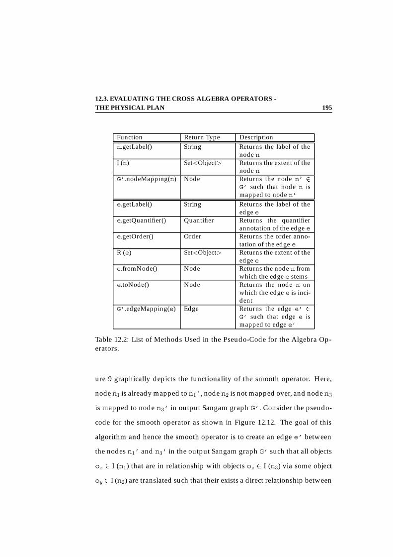
12.3. EVALUATING THE CROSS ALGEBRA OPERATORS -THE PHYSICAL PLAN 195
Function Return Type Descriptionn.getLabel() String Returns the label of the
node nI (n) Set<Object> Returns the extent of the
node nG’.nodeMapping(n) Node Returns the node n’ 2
G’ such that node n ismapped to node n’
e.getLabel() String Returns the label of theedge e
e.getQuantifier() Quantifier Returns the quantifierannotation of the edge e
e.getOrder() Order Returns the order anno-tation of the edge e
R (e) Set<Object> Returns the extent of theedge e
e.fromNode() Node Returns the node n fromwhich the edge e stems
e.toNode() Node Returns the node n onwhich the edge e is inci-dent
G’.edgeMapping(e) Edge Returns the edge e’ 2G’ such that edge e ismapped to edge e’
Table 12.2: List of Methods Used in the Pseudo-Code for the Algebra Op-erators.
ure 9 graphically depicts the functionality of the smooth operator. Here,
noden1 is already mapped to n1’, node n2 is not mapped over, and node n3
is mapped to node n3’ in output Sangam graph G’. Consider the pseudo-
code for the smooth operator as shown in Figure 12.12. The goal of this
algorithm and hence the smooth operator is to create an edge e’ between
the nodes n1’ and n3’ in the output Sangam graph G’ such that all objects
ox 2 I (n1) that are in relationship with objects oz 2 I (n3) via some object
oy 2 I (n2) are translated such that their exists a direct relationship between

12.3. EVALUATING THE CROSS ALGEBRA OPERATORS -THE PHYSICAL PLAN 196
Function Return Type Descriptionon.getValue() Value Returns the value of the
node objectoe.fromObject() NodeObject Returns the NodeObject
from which the edgeOb-ject oe stems.
oe.toObject() NodeObject Returns the NodeObjecton which the edgeObjectoe is incident.
ot.getParentObject() NodeObject Returns the NodeObjectfor which this object-tuple is defined. For ex-ample if ot = o:<o1, o2,. . ., on>, then getParen-tObject() returns o.
ot.getObject() NodeObject Returns the NodeObjectat index position in-dexPos in the Object-Tuple. The order of eachobject denotes the orderof the edges in whichthey participate.
Table 12.3: List of Methods Used in the Pseudo-Code for the Algebra Op-erators.
corresponding objects ox’ and oz’.
Let e1:<n1, n2> and e2:<n2, n3> be two edges between the nodes n1,
n2 and n3 2 G. The smooth operator creates a new edge e’ 2 G’ between
the nodes n1’ and n3’. For every edgeObject eo1:<o1, o2> 2 R (e1), we find
all the edgeObjects eo2:<oi, oj> 2 R (e2), such that oi = o2. The smooth
creates a new edgeObject oe:<o1’,oj’> for every eo2. The edgeObject
is inserted into the extent R (e’) of the new edge e’.

12.3. EVALUATING THE CROSS ALGEBRA OPERATORS -THE PHYSICAL PLAN 197
Function ReturnType
Description
op.hasChildren() Boolean Returns true of the oper-ator op has children op-erators. A child opera-tor is either related via acontext dependency re-lation or a derivation re-lation.
op.getNextChild() Operator Returns the next childoperator of the currentoperator op
op.evaluate() Sang-amgraph
Evaluates the operatorbased on the set of in-puts provided. Re-turns the output Sang-am graph. .
op.markDone() none Marks that the operatorhas been evaluated.
op.edgeType() String Returns the type of edgebetween the operator opand the passed in oper-ator. Valid answers arederivation or contextDe-pendency.
Table 12.4: List of Methods Used in the Algorithms for Evaluating CrossAlgebra Graphs.
12.3.2 Evaluating a Cross Algebra Graph
As presented in Section 12.2, the cross algebra graph consists of either con-
text dependency or derivation trees or a composition of context depen-
dency and derivation trees. Thus CAGs can be composed as a forest of
context dependency and derivation trees, a larger derivation or a larger
context dependency tree. Each tree CAT i of the CAG, called a CAT, can be
evaluated independently of any other tree CATj of the CAG. To evaluate

12.3. EVALUATING THE CROSS ALGEBRA OPERATORS -THE PHYSICAL PLAN 198
operator crossOp (input: Node n)
Node n’ insertNode ( n.getLabel(), τ )Extent I(n) scan (n)
NodeObject ox
I(n) .open ()while (ox I(n) .getNext ())
NodeObject ox’ copy (ox)write (ox’, I (n’))
I(n) .close ()
Figure 12.10: The Cross Physical Operator - An Implementation.
a CAT, we use post-order evaluation, i.e., all children operators opj of an
operator opk are evaluated prior to the evaluation of opk.
If the edge between the child operator opj and the parent operator opi
is a context dependency edge (denoted by the symbol “,” in the CAG ex-
pression), then the final output produced by the parent is a union of its
output and the output of all its context dependency children. Thus, in this
case outfinal = outiSoutj, where outfinal is the final output returned
by the parent operator opi, outi the local output of opi and outj is the
output returned by the child operator opj . To facilitate shared operators,
each operator opj is marked “visited” the first time it is evaluated, and its
local output is cached. If the operator opj is re-visited, no further evalua-
tion of opj is done, and its cached output is returned to the invoking parent
operator opi.
If the edge between the child operator opj and the parent operator opi
is a derivation edge (denoted by the symbol “( )” in the CAG expression),

12.3. EVALUATING THE CROSS ALGEBRA OPERATORS -THE PHYSICAL PLAN 199
operator connectOp (input: Sangam graph G, input Edge e:<n1, n2>,output: Sangam graph G’)
Node n1’ G’.nodeMapping(e.fromNode)Node n2’ G’.nodeMapping(e.toNode)
// Create a new edge and insert it into G’Edge e’ createSAGEdge( e.getLabel(), e.getQuantifier(), e.getOrder(),
n1’, n2’)G’.insertEdge (n1’, n2’, e’)
Extent Ie scan (e)
EdgeObject oe
Ie.open ()while (oe Ie.getNext ())
EdgeObject oe’ new EdgeObject ()oe’.fromObject G’.objectMapping(oe.fromObject)oe’.toObject G’.objectMapping(oe.toObject)write (oe’, R (e’))
Ie.close ()
Figure 12.11: The Connect Physical Operator - An Implementation.
then the output outj of the child operator opj is consumed directly by the
parent operator opi, i.e., output outj of the operator opj is the input ini
of the operator opi. The final output outfinal produced by opi in this case
is its own local output. Thus, in this case outfinal = outi, where outfinal
is the final output returned by the parent operator op i and outi the local
output of opi.
In both of the above cases (derivation and context dependency), in or-
der to facilitate shared operators, each operator opj is marked “visited”
the first time it is evaluated, and its local output is cached. If the operator

12.3. EVALUATING THE CROSS ALGEBRA OPERATORS -THE PHYSICAL PLAN 200
operator smoothOp (input: Sangam graph G, input: Edge e1:<n1, n2>,input: Edge e2:<n2, n3>, output: Sangam graph G’)
Node n1’ G’.nodeMaping(e1.fromNode)Node n3’ G’.nodeMapping(e2.toNode)
// Create a new edge and insert into G’Edge e’ createSAGEdge( e1.getLabel(), e1.getQuantifier()
e2.getQuantifier(), e1.getOrder(), n1’, n3’)
G’.insertEdge (n1’, n3’, e’)
Extent Ie1 scan (e1)Extent Ie2 scan (e2)
EdgeObject oe1
EdgeObject oe2
Ie1.open ()Ie2.open ()
while (oe1 Ie1.getNext ()) foreach (oe2 Ie2.getNext ())
if (oe1.toObject = oe2.fromObject) EdgeObject oe’ new EdgeObject ()oe’.fromObject G’.objectMapping(oe1.fromObject)oe’.toObject G’.objectMapping(oe2.toObject)write (oe’, R (e’))
Ie1.close ()Ie2.close ()
Figure 12.12: The Smooth Physical Operator - An Implementation.
opj is re-visited, no further evaluation of opj is done, and its cached out-
put is returned to the invoking parent operator op i. Evaluation of the tree
terminates with the evaluation of the root operator. Figure 12.14 gives the

12.3. EVALUATING THE CROSS ALGEBRA OPERATORS -THE PHYSICAL PLAN 201
operator subdivideOp (input: Edge e1:<n1, n3>, output: Sangam graph G’)
Node n1’ G’.nodeMapping(e1.fromNode)Node n3’ G’.nodeMapping(e1.toNode)
// Create the required Node and Edges and insert in G’Node n2’ createSAGNode( defaultLabel)Edge e1’ createSAGEdge( e1.getLabel(), e1.getQuantifier(), e1.getOrder(),
n1’, n2’)G’.insertNode (n2’)G’.insertEdge (n1’, n2’, e1’)
Edge e2’ createSAGEdge( e1.getLabel(), 0:1, 1, n2’, n3’)
G’.insertEdge (n2’, n3’, e2’)
Extent Re1 scan (e1)
Re1.open ()EdgeObject oe
while (oe Re1.getNext ())
NodeObject ox’ new NodeObject ()
EdgeObject oe’ new EdgeObject ()oe’.fromObject G’.nodeMapping(oe.fromObject)oe’.toObject ox’write (oe’, R (e1’))
EdgeObject of’ new EdgeObject ()of’.fromObject ox’of’.toObject G’.nodeMapping(oe.toObject)write (of’, R (e2’))
Re1.close ()
Figure 12.13: The SubDivide Operator - An Implementation.
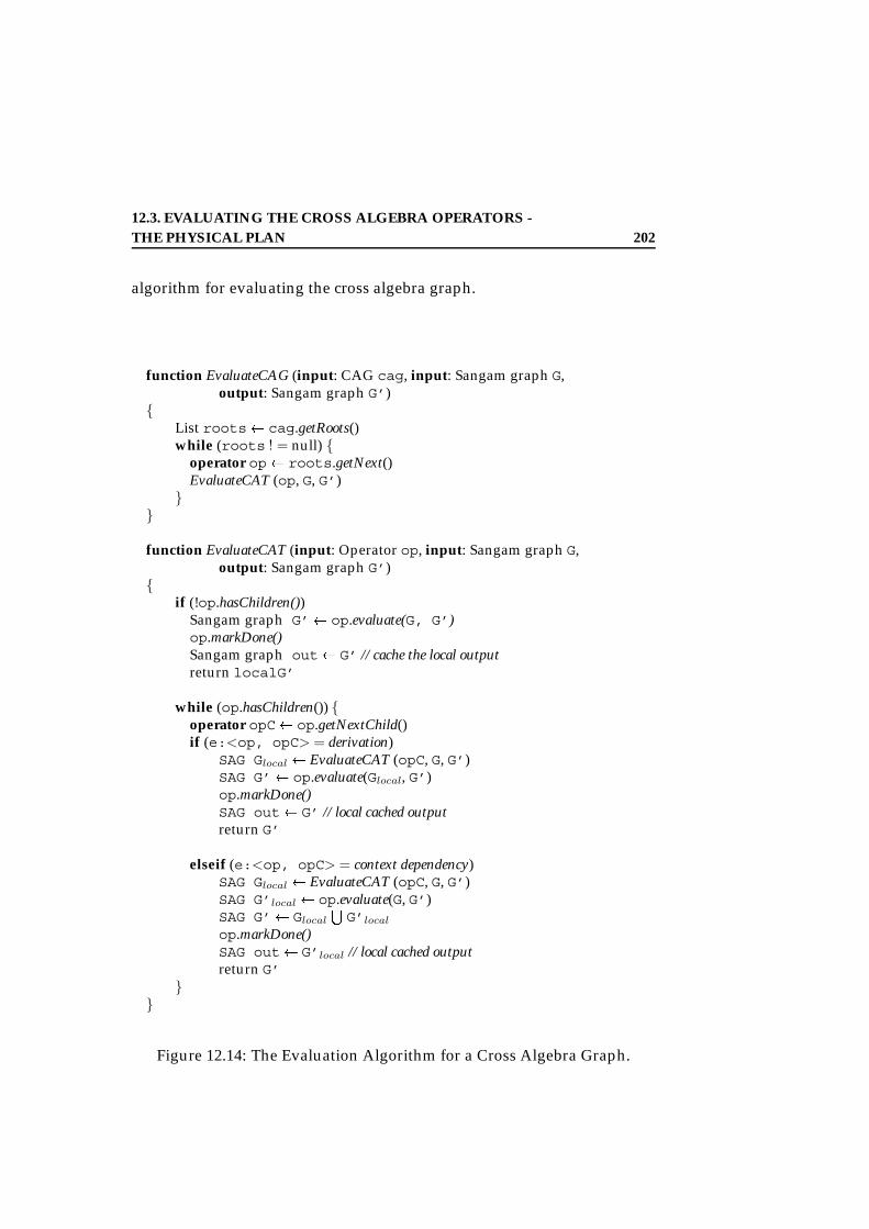
12.3. EVALUATING THE CROSS ALGEBRA OPERATORS -THE PHYSICAL PLAN 202
algorithm for evaluating the cross algebra graph.
function EvaluateCAG (input: CAG cag, input: Sangam graph G,output: Sangam graph G’)
List roots cag.getRoots()while (roots ! = null)
operator op roots.getNext()EvaluateCAT (op, G, G’)
function EvaluateCAT (input: Operator op, input: Sangam graph G,output: Sangam graph G’)
if (!op.hasChildren())
Sangam graph G’ op.evaluate(G, G’)op.markDone()Sangam graph out G’ // cache the local outputreturn localG’
while (op.hasChildren()) operator opC op.getNextChild()if (e:<op, opC> = derivation)
SAG Glocal EvaluateCAT (opC, G, G’)SAG G’ op.evaluate(Glocal, G’)op.markDone()SAG out G’ // local cached outputreturn G’
elseif (e:<op, opC> = context dependency)SAG Glocal EvaluateCAT (opC, G, G’)SAG G’local op.evaluate(G, G’)SAG G’ Glocal
SG’local
op.markDone()SAG out G’local // local cached outputreturn G’
Figure 12.14: The Evaluation Algorithm for a Cross Algebra Graph.

12.3. EVALUATING THE CROSS ALGEBRA OPERATORS -THE PHYSICAL PLAN 203
Evaluation Termination.
Lemma 8 (CAG Termination) The evaluation of a CAG as defined by Defini-
tion 19 will always terminate.
Proof: Let CAG represent a CAG as defined in Definition 19. For termina-
tion, we consider the following cases:
• Case 1 - CAG = CT: A context dependency tree CT expression is
evaluated from the right to left, that is from the leaf operators (chil-
dren operators) to the parent operator. As each context dependency
tree CT has at most one root and CT is free of cycles (Lemma 5), the
evaluation of CT terminates when the root operator is evaluated.
• Case 2 - CAG = DT: A derivation tree DT expression is evaluated
from the inner most operator, represented as leaves of the tree, to the
outermost operator, the root of the tree. Evaluation terminates when
the root operator is evaluated. Again, as a derivation tree contains no
cycles (Lemma 4), the evaluation is always guaranteed to terminate.
• Case 3 - CAG = opi, (CAGj): opi,(CAGj) represents a context de-
pendency tree where opi is the root of the CAG CAGj, such that there
exists a context dependency edge from the root operator op i to the
root opj of the CAG CAGj.
1. CAGj = CT: In this case CAG represents a large but pure context
dependency tree such that the operator op i is the root of the tree.
This thus reduces to Case 1. Hence the evaluation of CAG will
always terminate in this case.
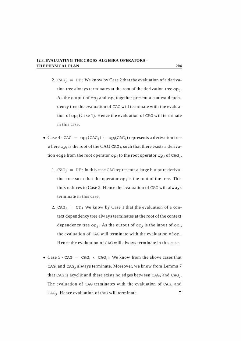
12.3. EVALUATING THE CROSS ALGEBRA OPERATORS -THE PHYSICAL PLAN 204
2. CAGj = DT:We know by Case 2 that the evaluation of a deriva-
tion tree always terminates at the root of the derivation tree opj .
As the output of opj and opi together present a context depen-
dency tree the evaluation of CAG will terminate with the evalua-
tion of opi (Case 1). Hence the evaluation of CAG will terminate
in this case.
• Case 4 - CAG = opi(CAGj)): opi(CAGj) represents a derivation tree
where opi is the root of the CAG CAGj, such that there exists a deriva-
tion edge from the root operator opi to the root operator opj of CAGj.
1. CAGj = DT: In this case CAG represents a large but pure deriva-
tion tree such that the operator opi is the root of the tree. This
thus reduces to Case 2. Hence the evaluation of CAG will always
terminate in this case.
2. CAGj = CT: We know by Case 1 that the evaluation of a con-
text dependency tree always terminates at the root of the context
dependency tree opj . As the output of opj is the input of opi,
the evaluation of CAG will terminate with the evaluation of opi.
Hence the evaluation of CAG will always terminate in this case.
• Case 5 - CAG = CAGi Æ CAGj: We know from the above cases that
CAGi and CAGj always terminate. Moreover, we know from Lemma 7
that CAG is acyclic and there exists no edges between CAGi and CAGj.
The evaluation of CAG terminates with the evaluation of CAGi and
CAGj. Hence evaluation of CAG will terminate. 2
12.4. AN EXAMPLE 205
12.4 An Example
Shanmugasundaram et al. [STZ+99] have proposed the basic inlining tech-
nique for translating an XML DTD and associated document into a rela-
tional schema and data. In this section, we describe the basic inlining tech-
nique and then show how it can be represented by a cross algebra graph.
12.4.1 The Basic Inlining
The Basic Inlining Technique. For each element, the basic inlining tech-
nique inlines as many descendants of an element as possible into a single
relation. However, as an XML document can be rooted at any element, this
technique is applied for all elements in a DTD and hence creates relations
for every element. As an example consider the XMark benchmark DTD
given in Figure 10.2. Here the item element would be mapped to a rela-
tion with attributes location, mailbox and name. Set-valued attributes
such as the attribute mail in element mailbox are stored following the
standard technique for storing sets in a RDBMS. Hence, a relation is cre-
ated for the mail attribute and it is linked to the mailbox using a foreign
key. Figure 12.15 shows the relational schema obtained by applying the
basic inlining technique to the fragment of XMark benchmark DTD in Fig-
ure 10.2.
Shanmugasundaram et al. [STZ+99] present an algorithm that first
converts a given DTD into an element graph. This element graph is con-
structed as follows. Do a depth first traversal of the DTD graph, starting at
the element node for which the relations are being constructed. Each node
12.4. AN EXAMPLE 206
is marked as “visited” the first time it is reached and is unmarked once all
its children have been traversed.
If an unmarked node in the DTD graph is reached during the depth
first traversal, a new node bearing the same name is created in the element
graph. In addition, a regular edge is created from the most recently created
node in the element graph with the same name as the DFS parent of the
current DTD node to the newly created node.
If an attempt is made to traverse an already marked DTD node, then a
backpointer edge is added from the most recently created node in the DTD
graph to the most recently created node in the element graph with the same
name as the marked DTD node.
In general, given an element graph, relations are created as follows. A
relation is created for the root element of the graph. All the element’s de-
scendants are inlined into that relation with the following two exceptions:
(a) children with a “*” are made into separate relations - this corresponds
to creating a new relation for a set-valued child; and (b) to handle recur-
sion within elements, each node in the element graph having a backpointer
edge is made into a separate relation. For further details we refer the reader
to [STZ+99].
Cross Algebra Graph for Basic Inlining. To construct the basic inlin-
ing technique as a cross algebra graph (CAG) we follow a simple algo-
rithm. Given an input Sangam graph that represents the element graph
constructed using the algorithm above [STZ+99], we create:
1. cross () operators for every node in the Sangam graph. This includes
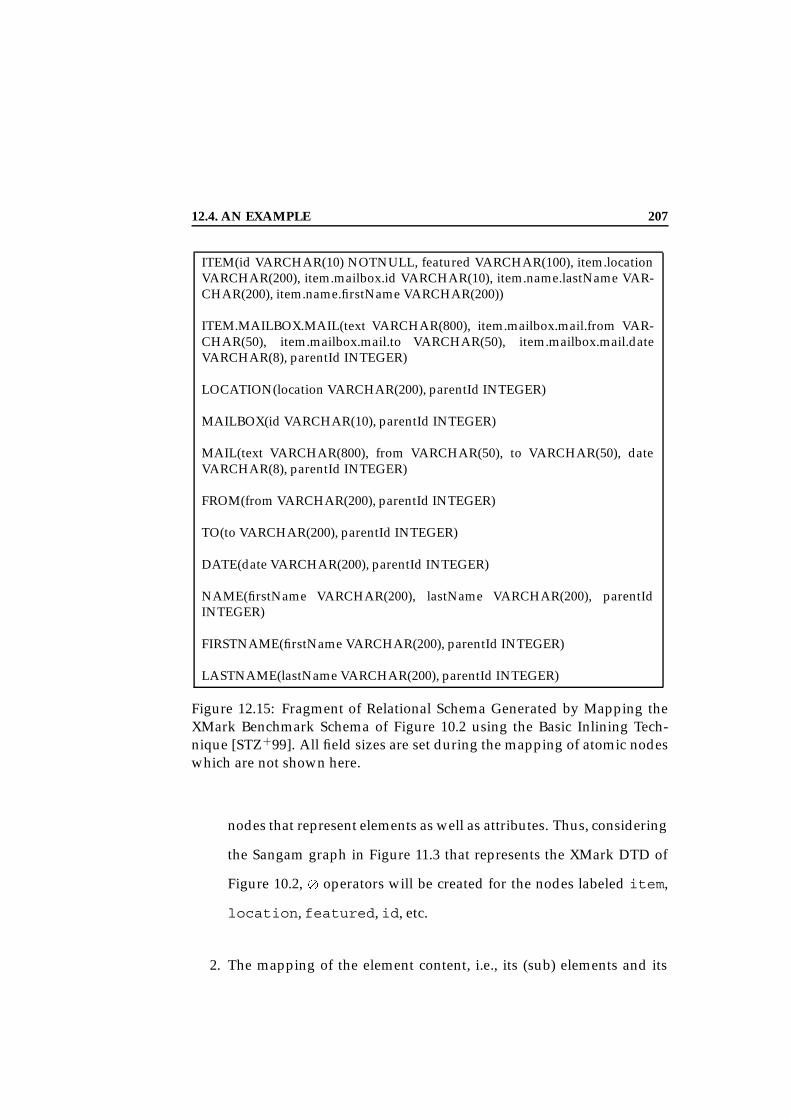
12.4. AN EXAMPLE 207
ITEM(id VARCHAR(10) NOTNULL, featured VARCHAR(100), item.locationVARCHAR(200), item.mailbox.id VARCHAR(10), item.name.lastName VAR-CHAR(200), item.name.firstName VARCHAR(200))
ITEM.MAILBOX.MAIL(text VARCHAR(800), item.mailbox.mail.from VAR-CHAR(50), item.mailbox.mail.to VARCHAR(50), item.mailbox.mail.dateVARCHAR(8), parentId INTEGER)
LOCATION(location VARCHAR(200), parentId INTEGER)
MAILBOX(id VARCHAR(10), parentId INTEGER)
MAIL(text VARCHAR(800), from VARCHAR(50), to VARCHAR(50), dateVARCHAR(8), parentId INTEGER)
FROM(from VARCHAR(200), parentId INTEGER)
TO(to VARCHAR(200), parentId INTEGER)
DATE(date VARCHAR(200), parentId INTEGER)
NAME(firstName VARCHAR(200), lastName VARCHAR(200), parentIdINTEGER)
FIRSTNAME(firstName VARCHAR(200), parentId INTEGER)
LASTNAME(lastName VARCHAR(200), parentId INTEGER)
Figure 12.15: Fragment of Relational Schema Generated by Mapping theXMark Benchmark Schema of Figure 10.2 using the Basic Inlining Tech-nique [STZ+99]. All field sizes are set during the mapping of atomic nodeswhich are not shown here.
nodes that represent elements as well as attributes. Thus, considering
the Sangam graph in Figure 11.3 that represents the XMark DTD of
Figure 10.2, operators will be created for the nodes labeled item,
location, featured, id, etc.
2. The mapping of the element content, i.e., its (sub) elements and its

12.4. AN EXAMPLE 208
attributes, is represented by a collection of connect, smooth and sub-
divide nodes. Here, the path p from a given node m to another node
n is given by a sequence of edges p = e1.e2.. . ..en. The size of the
path p, jpj = n. We ignore the backpointer edges unless explicitly
specified. In the steps below, we calculate the path from given node
m to a leaf node. Recall that a leaf node is any node n that only has
atomic children ( 11). For clarity of the algorithm given below, we
assume here that a leaf is also any node n such that the quantifier
annotation on the edge e:<m, n> is either [0:i] or [1:i], i 6= 0 or
1 9, and the node m is the parent node. For each path p = e1.e2.. . ..en
we do:
• if p = e1, and jpj 1 then, create a connect () operator that
maps the edge e1:<m, n> to an edge e1’ in the output Sangam
graph G’. Context dependency edges are built from the connect
operator to the cross operator that maps the node m as well as to
the cross operator that maps the node n. Consider the Sangam
graph in Figure 12.16. Here a operator is created for the edge
between the nodes labeled item and location. Also the
operator will have a context dependency edge to the operators
that map these nodes item and location. Figure 12.17 depicts
the context dependency tree produced by the above step for the
input Sangam graph G in Figure 12.16, while Figure 12.18 shows
the output Sangam graph G’.
9In XML terms this would be any element with a + or .
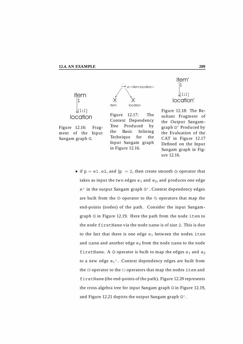
12.4. AN EXAMPLE 209
Figure 12.16: Frag-ment of the InputSangam graph G.
Figure 12.17: TheContext DependencyTree Produced bythe Basic InliningTechnique for theInput Sangam graphin Figure 12.16.
Figure 12.18: The Re-sultant Fragment ofthe Output Sangam-graph G’ Produced bythe Evaluation of theCAT in Figure 12.17Defined on the InputSangam graph in Fig-ure 12.16.
• if p = e1.e2, and jpj = 2, then create smooth = operator that
takes as input the two edges e1 and e2, and produces one edge
e’ in the output Sangam graph G’. Context dependency edges
are built from the = operator to the operators that map the
end-points (nodes) of the path. Consider the input Sangam-
graph G in Figure 12.19. Here the path from the node item to
the node firstName via the node name is of size 2. This is due
to the fact that there is one edge e1 between the nodes item
and name and another edge e2 from the node name to the node
firstName. A = operator is built to map the edges e1 and e2
to a new edge e1’. Context dependency edges are built from
the = operator to the operators that map the nodes item and
firstName (the end-points of the path). Figure 12.20 represents
the cross algebra tree for input Sangam graph G in Figure 12.19,
and Figure 12.21 depicts the output Sangam graph G’.
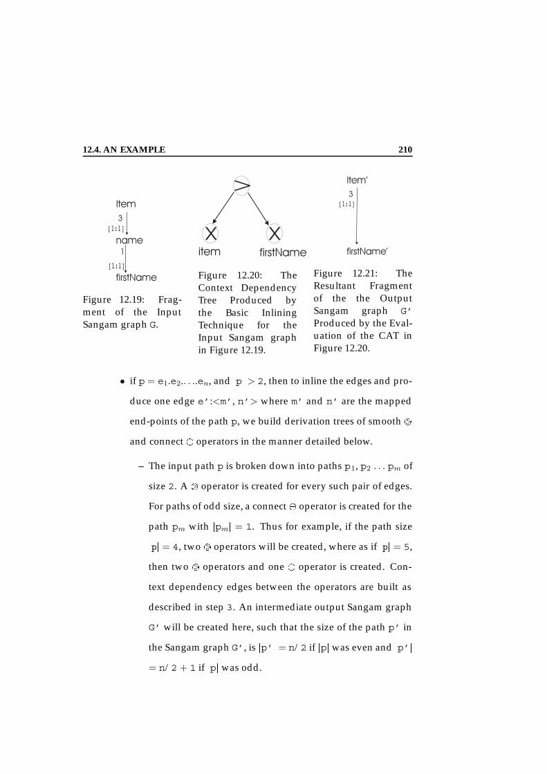
12.4. AN EXAMPLE 210
Figure 12.19: Frag-ment of the InputSangam graph G.
Figure 12.20: TheContext DependencyTree Produced bythe Basic InliningTechnique for theInput Sangam graphin Figure 12.19.
Figure 12.21: TheResultant Fragmentof the the OutputSangam graph G’Produced by the Eval-uation of the CAT inFigure 12.20.
• if p = e1.e2.. . ..en, and jpj > 2, then to inline the edges and pro-
duce one edge e’:<m’, n’> where m’ and n’ are the mapped
end-points of the path p, we build derivation trees of smooth =
and connect operators in the manner detailed below.
– The input path p is broken down into paths p1, p2 . . . pm of
size 2. A = operator is created for every such pair of edges.
For paths of odd size, a connect operator is created for the
path pm with jpmj = 1. Thus for example, if the path size
jpj = 4, two = operators will be created, where as if jpj = 5,
then two = operators and one operator is created. Con-
text dependency edges between the operators are built as
described in step 3. An intermediate output Sangam graph
G’ will be created here, such that the size of the path p’ in
the Sangam graph G’, is jp’j = n/2 if jpjwas even and jp’j
= n/2 + 1 if jpj was odd.

12.4. AN EXAMPLE 211
– Next, to further inline the path p’ and to produce a path
pn/4 of size n/4, one = operator ops is created for every
pair of = and operators op1, op2 created in the previous
step. A derivation edge is built from the operators op1 and
op2 to the operator ops to indicate that the operator’s inputs
are the outputs of the two operators op1 and op2.
– The above step is repeated until the an output Sangam graph
G’ is produced with a path pn of size 1.
– As a last step, we create the context dependency edges from
the root of the CAT (this is operator with the final output of
one edge) to the two end-points of the edge as described in
step 3.
Consider the input Sangam graph fragment G shown in Fig-
ure 12.22. To inline the leaf nodefirstName, we create a smooth
= operator op1 that maps the input edges e1:<item, name>,
and e2:<name, first>. This produces the intermediate edge
e’<item, first>. A connect operator op2 maps over the
edge e3:<first, firstName>. The output of this operator,
edge e’’:<first, firstName> and the output of op1 become
input edges for smooth (=) operator op3 that produces edge
e’’’:<item, first>. The expression for the cross algebra
graph CAG in Figure 12.23 is given as: CAG= (op6e0 (CT1, CT2)),
(op1item0(item) Æ op3firstName0(firstName))). the context de-
pendency tree CT1 is given as CT1 = (op4e1Temp(e1: <item,
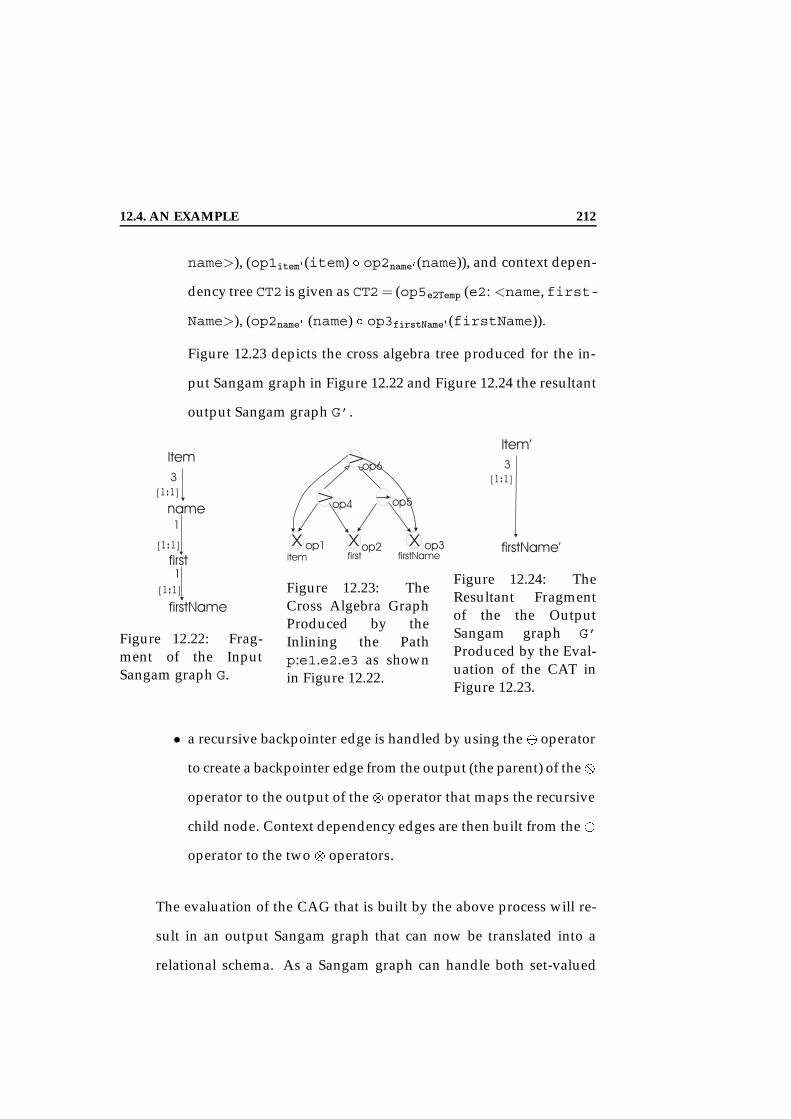
12.4. AN EXAMPLE 212
name>), (op1item0(item) Æ op2name0(name)), and context depen-
dency tree CT2 is given as CT2= (op5e2Temp (e2: <name,first-
Name>), (op2name0 (name) Æ op3firstName0(firstName)).
Figure 12.23 depicts the cross algebra tree produced for the in-
put Sangam graph in Figure 12.22 and Figure 12.24 the resultant
output Sangam graph G’.
Figure 12.22: Frag-ment of the InputSangam graph G.
Figure 12.23: TheCross Algebra GraphProduced by theInlining the Pathp:e1.e2.e3 as shownin Figure 12.22.
Figure 12.24: TheResultant Fragmentof the the OutputSangam graph G’Produced by the Eval-uation of the CAT inFigure 12.23.
• a recursive backpointer edge is handled by using the operator
to create a backpointer edge from the output (the parent) of the
operator to the output of the operator that maps the recursive
child node. Context dependency edges are then built from the
operator to the two operators.
The evaluation of the CAG that is built by the above process will re-
sult in an output Sangam graph that can now be translated into a
relational schema. As a Sangam graph can handle both set-valued

12.4. AN EXAMPLE 213
Figure 12.25: A Fragment of the XMark Benchmark DTD as shown in Fig-ure 10.2 Depicted as a Sangam Graph (Sangam graph ). No order and quan-tifier annotations are shown for the backpointer edges to distinguish themin the figure. These are defaulted to 1 and [1:1] respectively.
attributes as well as recursion, we do not have to handle these when
building the cross algebra graph (CAG). Instead, the issue of translat-
ing the set-valued attributes and recursion is handled when a Sang-
am graph is translated into a relational schema as discussed in Sec-
tion 11.2.2. Figure 12.26 graphically depicts the CAG that translates
the Sangam graph in Figure 12.25 to the Sangam graph shown in Fig-
ure 12.27.
The Sangam graph in Figure 12.27 can now be translated based on the
steps given in Section 11.2.2 to a relational schema is as shown in Fig-
ure 12.28.

12.4. AN EXAMPLE 214
Figure 12.26: The Cross Algebra Graph that represents the Basic InliningTechnique applied to the Sangam graph in Figure 11.3. This Sangam graphis only for the node with root item. Cross Algebra Trees similar to the onesgiven in this figure will be produced for each root node.
12.4.2 The Shared Inlining
Shared Inlining Technique. The principal idea behind shared inlining is
to identify the elements that would be represented by multiple relations by
the basic inlining technique, and then to share them by creating separate
relations for these elements. In this technique, relations are created for all
elements in the DTD graph that have an in-degree greater than one. Nodes
with in-degree of one are inlined and the nodes with in-degree of zero are
made into separate relations. Mutually recursive elements are handled the
same as in the basic inlining approach.
CAG for Shared Inlining Technique. The algorithm for creating a CAG
for the shared inlining technique is similar to that of creating the CAG for
a basic inlining with a few differences. The main difference is that in the

12.4. AN EXAMPLE 215
Figure 12.27: Output Sangam graph Produced by the Evaluation of theCross Algebra Graph in Figure 12.26 for Input Sangam graph in Fig-ure 12.25.
Item’(id’ VARCHAR(10) NOTNULL, featured’ VARCHAR(100) NOTNULL,location’ VARCHAR(200) NOTNULL, firstName’ VARCHAR(200), lastName’VARCHAR(200))
Item.mail’(from’ VARCHAR(50), to’ VARCHAR(50), date’ VARCHAR(8),CONSTRAINT fk id FOREIGN KEY (id’) REFERENCES Item’(id’))
Figure 12.28: The Relational Schema Produced by the Translation of theSangam graph in Figure 12.27.

12.5. SUMMARY 216
CAG for basic inlining all nodes are mapped to the output via opera-
tors. For example, the node item and location are mapped and pro-
duce output nodes item’ and location’. A operator is then used to
re-create the edge e1 between item and location to now exist between
the nodes item’ and location’. In addition all the sub-elements of the
node location obtained by following the backpointer edge are inlined
as direct children of the node location’. In addition, the node location
representing a possible root is also mapped as such to the output. In shared
inlining, this root node location is mapped to the output only if the num-
ber of backpointer edges for this node is greater than one, or if they are zero.
All nodes with only one backpointer edge are inlined and no separate cross
algebra tree is created to map it to the output. The rest of the algorithm
remains the same as the basic inlining algorithm.
12.5 Summary
In this chapter, we have presented the basic transformation components of
the Sangam middle-layer, and shown how a local application schema can
be mapped from one data model to a schema in another data model via the
Sangam middle-layer. To enable this transformation across data models, in
this chapter we have defined (1) the primitive set of cross algebra operators
that conform to the set of linear transformation operators [GY98]. These
operators have been shown in graph transformation literature [GY98] to be
sufficiently powerful to express complex transformations, and to be suffi-
cient to express all linear transformations; (2) two different techniques of

12.5. SUMMARY 217
composing algebra expression for these operators; (3) the physical binding
and the evaluation algorithm for these operators; and (4) a concrete exam-
ple that transforms the XMark [SWK+01] benchmark schema to a relational
schema via the basic and shared inlining methods [STZ+99]. These tech-
niques are represented by a cross algebra expression in the Sangam middle
layer.
Our work on cross-algebra as a generic mapping language has signifi-
cant advantages.
• Re-usable transformations. With the cross algebra, we are able to de-
fine many basic and complex transformations such as, the inlining of
an XML schema into a relational schema. This cross algebra expres-
sion is not bound to any particular XML schema or relational schema,
but rather can now be re-used to perform the inlining transformation
between any two Sangam graphs.
• Development of Re-usable tools. Tools such as propagation algorithms,
optimization strategies can now be developed based on the cross al-
gebra expressions. These tools are re-usable for any cross algebra ex-
pression defined between schemas for any data model.
In the next Chapter, we provide the description of one such tool, the
propagation algorithm, that can propagate change from the XML input to
the relational output via the Sangam integration framework.

12.5. SUMMARY 218

219
Chapter 13
Sangam: Evaluating the Theory
Based on the concepts of the Sangam graph model and the Cross Algebra
Graph presented in Chapters 11 and 7 respectively, we have developed
a middle-layer framework that can translate XML DTDs and documents
to relational schemas and data via cross algebra graphs that can represent
a variety of translation techniques. In this chapter, we present the over-
all architecture of the prototype system Sangam as well as a performance
calibration of the various components of the Sangam architecture.
13.1 Architectural Overview of Cross Algebra Process-
ing Engine
Figure 13.1 depicts the architecture and the data flow of our prototype sys-
tem, Sangam. This system has been developed using Java technology and
a variety of tools such as the JAXP [Sys01] for parsing XML documents and
the DTD-Parser [Wut01] for parsing the DTDs.
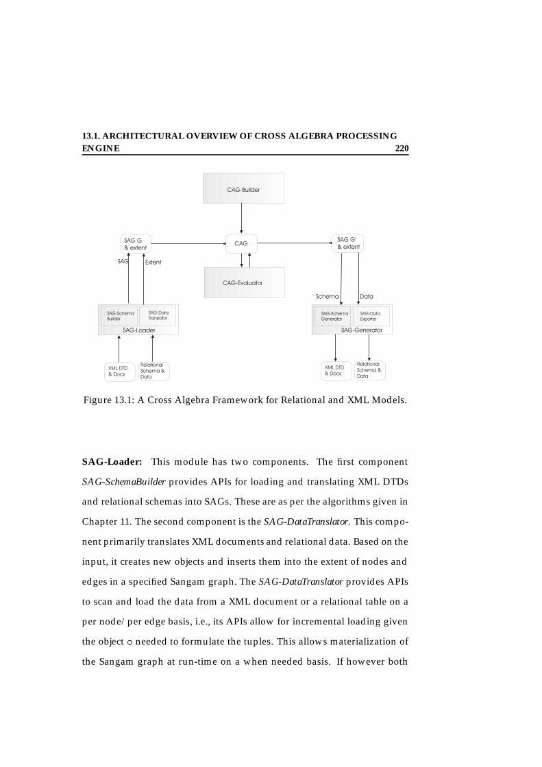
13.1. ARCHITECTURAL OVERVIEW OF CROSS ALGEBRA PROCESSINGENGINE 220
Figure 13.1: A Cross Algebra Framework for Relational and XML Models.
SAG-Loader: This module has two components. The first component
SAG-SchemaBuilder provides APIs for loading and translating XML DTDs
and relational schemas into SAGs. These are as per the algorithms given in
Chapter 11. The second component is the SAG-DataTranslator. This compo-
nent primarily translates XML documents and relational data. Based on the
input, it creates new objects and inserts them into the extent of nodes and
edges in a specified Sangam graph. The SAG-DataTranslator provides APIs
to scan and load the data from a XML document or a relational table on a
per node/per edge basis, i.e., its APIs allow for incremental loading given
the object o needed to formulate the tuples. This allows materialization of
the Sangam graph at run-time on a when needed basis. If however both

13.1. ARCHITECTURAL OVERVIEW OF CROSS ALGEBRA PROCESSINGENGINE 221
components are invoked during the initial load, then a fully materialized
Sangam graph will be generated.
CAG-Builder: This module is responsible for building a cross algebra
graph based on either the basic inlining or shared inlining technique and
a given input Sangam graph. These CAGs are built as per the algorithms
outlined in Section 12.4. Thus, the CAG-Builder takes as input a Sangam
graph, and a parameter that specifies either the basic inlining or the shared
inlining techniques. The output of this module is a CAG for the specified
input Sangam graph G.
CAG-Evaluator: The core of the system lies in the CAG-Evaluator. Once
a CAG has been built by the CAG-Builder, this module is responsible for
generating the actual physical plan, executing the plan and hence produc-
ing the output Sangam graph and its translated data. Physical algebra op-
erators and the evaluation algorithm are a core part of this module. Details
of these are given in Chapter 12.3.
SAG-Generator: The SAG-Generator is responsible for generating the ac-
tual application schemas and for translating the Sangam graph data into a
specific data model. As in the SAG-Loader module, there are two main
components to this module: SAG-SchemaGenerator and SAG-DataExporter.
The module SAG-SchemaGenerator can take a given Sangam graph and gen-
erate either an XML DTD or a relational schema as output. This is a user-
specific choice and is specified at run-time via a parameter. The algorithm
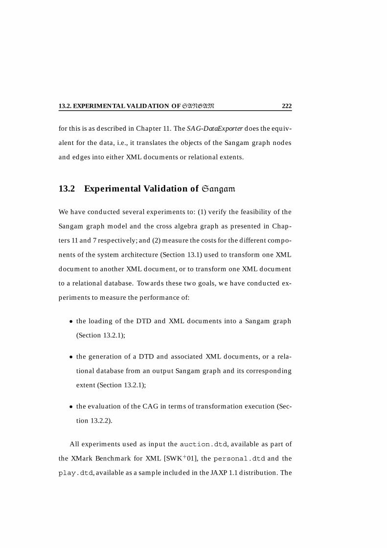
13.2. EXPERIMENTAL VALIDATION OF SANGAM 222
for this is as described in Chapter 11. The SAG-DataExporter does the equiv-
alent for the data, i.e., it translates the objects of the Sangam graph nodes
and edges into either XML documents or relational extents.
13.2 Experimental Validation of Sangam
We have conducted several experiments to: (1) verify the feasibility of the
Sangam graph model and the cross algebra graph as presented in Chap-
ters 11 and 7 respectively; and (2) measure the costs for the different compo-
nents of the system architecture (Section 13.1) used to transform one XML
document to another XML document, or to transform one XML document
to a relational database. Towards these two goals, we have conducted ex-
periments to measure the performance of:
• the loading of the DTD and XML documents into a Sangam graph
(Section 13.2.1);
• the generation of a DTD and associated XML documents, or a rela-
tional database from an output Sangam graph and its corresponding
extent (Section 13.2.1);
• the evaluation of the CAG in terms of transformation execution (Sec-
tion 13.2.2).
All experiments used as input the auction.dtd, available as part of
the XMark Benchmark for XML [SWK+01], the personal.dtd and the
play.dtd, available as a sample included in the JAXP 1.1 distribution. The

13.2. EXPERIMENTAL VALIDATION OF SANGAM 223
XML documents corresponding to the auction.dtd were generated us-
ing xmlgen, available for download from XMark [SWK+01]. The xmlgen tool
however can generate XML documents corresponding to theauction.dtd
only. Hence, to generate XML documents corresponding topersonal.dtd,
we wrote our own tool, called xmlPGen. A feature of the xmlPGen tool was
that it allowed us to produce a uniform distribution of the number of ob-
jects for all nodes and edges of the Sangam graph. The auction.dtd and
the personal.dtd are given in Appendix A.
For each input Sangam graph, we built (using the CAG-Builder) the
Cross Algebra Graphs (CAGs) that represent either (1) an identical, called
ident, transformation, in which case the input Sangam graph is identical to
the output Sangam graph; or (2) a basic inline, called inline, transformation
that models the basic inline technique presented by Shanmugasundaram
et al. [STZ+99]; or (3) a shared inline transformation that models the shared
inline technique [STZ+99]1.
All experiments were conducted on a Pentium IV, 933MHz, 256Mb RAM
system running Debian Linux, kernel version 2.2.19, using the Sangam pro-
totype system described in Section 13.1. The Sangam system itself was built
using the Java JDK, version 1.3.1. To store generated relational schemas and
data we used Oracle 9i running on Debian Linux, kernel version 2.2.19.

13.2. EXPERIMENTAL VALIDATION OF SANGAM 224
0
2000
4000
6000
8000
10000
12000
1 2 3 4 5 6
Tim
e in
Mill
isec
onds
XML Size in Megabytes
Loading Time vs. XML Size
XML Load TimeXML Load Time 95% confidence
DTD Load Time
Figure 13.2: Time Taken to Load the auction.dtd and auction.xmlDocuments of Varying Sizes Into the Sangam Graph.
13.2.1 Loading to and Generating from Sangam Graphs
Figure 13.2 depicts the time taken to translate a given DTD and load its
corresponding XML documents to a Sangam graph. We kept the DTD
auction.dtd constant, and increased the size of the XML documents
from 1MB to 7MB. Each data point represents the average of ten runs,
shown with 95% confidence intervals. As shown in the figure, the load
times of the DTD itself are a small fraction of the time required to load an
XML document. As seen by the slope of the XML load time, an increase in
the size of the XML document causes a linear increase in the time taken to
load the XML document into the Sangam graph. The SAG-DataTranslator
1We found the loading time of the basic and shared inlining to be almost identical. Wethus report only the results of the basic inlining.

13.2. EXPERIMENTAL VALIDATION OF SANGAM 225
0
500
1000
1500
2000
2500
play auction personal
Tim
e in
Mill
isec
onds
Comparison of the Load Times for Different DTDs and XML Files
dtd xml dtd xml dtd xml
Figure 13.3: Comparing the Load Times for Different DTDs and Corre-sponding XML Documents.
algorithm creates one nodeObject per XML element, and a fixed number
of edgeObjects representing the cardinality of the relationship between the
element and the sub-elements (or its attributes).
Figure 13.3 depicts a bar-chart graph showing the different load times
for three different DTDs, personal.dtd, auction.dtd and play.dtd
and their corresponding XML documents personal.xml,auction.xml,
and play.xml respectively. The auction.dtdwas the largest with a size
of 4k bytes. The personal.dtd and play.dtd were 0.5K and 1K re-
spectively. The auction.xml, personal.xml and play.xml were 3MB,
1MB and 27K respectively. These times were consistent with our hypothesis
that the loading times increase with the increase in size of the DTD and the
XML documents.

13.2. EXPERIMENTAL VALIDATION OF SANGAM 226
0
1000
2000
3000
4000
5000
6000
7000
8000
9000
10000
1 2 3 4 5 6
Tim
e in
Mill
isec
onds
XML Size in Megabytes
Generation Time vs. XML Size
XML Generate TimeDTD Generate Time
Figure 13.4: Time Taken to Generate the auction.dtd and Differentauction.xmlDocuments of Varying Sizes From a Given Sangam Graph.
Figure 13.4 depicts the time to generate DTD and XML documents from
a given Sangam graph. The Sangam graph structure used for the gen-
eration was initially loaded from auction.dtd and was kept constant.
We varied the extent size of the nodes and edges in the Sangam graph.
The different extent sizes for the Sangam graph were obtained by loading
XML documents of varying sizes, from 1MB to 7MB, as the extent of the
Sangam graph. To generate the DTD and XML documents, we performed
a depth first traversal of the Sangam graph and loaded appropriate objects
of the DTDParser [Wut01] and javax.xml.transform.Transformer
provided as part of the JAXP 1.1 [Sys01] package, respectively. The actual
generation of the DTD and the XML documents was done via the DTD-
Parser [Wut01] and the JAXP 1.1 Transformer [Sys01]. In this experiment,

13.2. EXPERIMENTAL VALIDATION OF SANGAM 227
0
2000
4000
6000
8000
10000
12000
1 2 3 4 5 6
Tim
e in
Mill
isec
onds
XML Size in Megabytes
Comparing the Load and Generation Times
XML Generate TimeDTD Generate Time
XML Load TimeDTD Load Time
Figure 13.5: Comparison of the Time Taken to Load and Generate theauction.dtd and Different auction.xml Documents of Varying Sizesto and from a Sangam Graph.
we report the total time for the generation of the DTD and the XML docu-
ments, including the DTDParser generation and the JAXP generation. As
shown in the figure, the generation times for the DTD are a small fraction
of the time required to generate an XML document. However, these gen-
eration times are considerably smaller than the load values. The difference
between the load and generate times can be attributed to the fact that the
generation algorithms require only one-pass through the Sangam graph, as
opposed to two passes need during the load process. Figure 13.5 compares
the time taken to load and generate the auction.dtd and auction.xml
to and from the Sangam graph.

13.2. EXPERIMENTAL VALIDATION OF SANGAM 228
13.2.2 CAG Evaluation
Performance of Cross Algebra Operators
Figure 13.6 depicts the time taken to evaluate one Cross algebra operator.
We kept the operator Cross and its input node constant, and increased
the extent of the input node from 1 to 20,000 objects. Each data point
represents the average of ten runs. The evaluation time of a Cross operator
increases linearly with a linear increase in the extent size of the input node.
0
100
200
300
400
500
600
700
800
0 2000 4000 6000 8000 10000 12000 14000 16000
Tim
e in
Mill
isec
onds
Input Node Extent: Number of Objects
Cross Evaluation Time vs. Cross Input Node Extent
Cross Operator Evaluation Time
Figure 13.6: The Time Taken to Evaluate a Cross Algebra Operator as theExtent Size of its Input is Varied.
Figure 13.7 depicts the time taken to evaluate one Connect algebra op-
erator. We kept the operator Connect and its input edge constant, and
increased the extent of the input edge from 1 to 20,000 edge objects. Each
data point represents the average of ten runs. The data in Figure 13.7 can

13.2. EXPERIMENTAL VALIDATION OF SANGAM 229
0
20000
40000
60000
80000
100000
120000
140000
160000
180000
0 2000 4000 6000 8000 10000 12000 14000 16000 18000 20000
Tim
e in
Mill
isec
onds
Input Edge Extent: Number of Objects
Connect Evaluation Time vs. Connect Input Edge Extent
Connect Operator Evaluation Time
Figure 13.7: The Time Taken to Evaluate a Connect Algebra Operator as theExtent Size of its Input is Varied.
be well represented by a polynomial2 with degree 2 with a coefficient of
determination3 of .99. Construction of one object of a connect operator
requires searching through the objects of the two nodes that represent the
end-points of the output edge. The evaluation time for the connect oper-
ator is thus O(n2). This is supported by our experimental results.
Figure 13.8 depicts the time taken to evaluate one Smooth operator. We
kept the Smooth operator and its two input edges constant, and uniformly
increased the extent of both its input edges from 1 to 20,000 edge ob-
jects. Each data point represents the average of ten runs, shown with 95%
2The exact polynomial function is: 0.0004x2 0.6x + 300.
3The coefficient of determination, also known as the R-squared value, is an indicatorthat ranges in value from 0 to 1 and reveals how closely the estimated values for the trendline correspond to the actual data. A trend line is most reliable when its coefficient of deter-mination is at or near 1.

13.2. EXPERIMENTAL VALIDATION OF SANGAM 230
0
50000
100000
150000
200000
250000
300000
0 2000 4000 6000 8000 10000 12000 14000 16000 18000 20000
Tim
e in
Mill
isec
onds
Number of Objects
Smooth Evaluation Time vs. Smooth Input Edges Extent
Smooth Operator Evaluation Time
Figure 13.8: The Time Taken to Evaluate a Smooth Algebra Operator as theExtent Size of its Inputs is Varied.
confidence intervals. The data in Figure 13.8 can be well represented by a
polynomial4 with degree 3 with a coefficient of determination of .998. Con-
struction of one object of a smooth operator requires searching through the
objects of the first node, determining all objects of the second node to which
it is connected, and then for each object of the second node determining all
the objects of the third node to which it is connected, leading to evaluation
times O(n3). This analysis for the evaluation times for the smooth operator
is supported by our experimental results.
Figure 13.9 depicts the time taken to evaluate one Subdivide oper-
ator. We kept the Subdivide operator and its input edge constant, and
increased uniformly the extent of its input edge from 1 to 20,000 edge
4The exact polynomial function is: 2e0.08x3 + 0.0002x2 + 1.1523x 283.81.

13.2. EXPERIMENTAL VALIDATION OF SANGAM 231
0
500000
1e+06
1.5e+06
2e+06
2.5e+06
0 2000 4000 6000 8000 10000 12000 14000 16000 18000 20000
Tim
e in
Mill
isec
onds
Input Edge Extent: Number of Objects
Subdivide Evaluation Time vs. Subdivide Input Edge Extent
Subdivide Operator Evaluation Time
Figure 13.9: The Time Taken to Evaluate a Subdivide Algebra Operator asthe Extent Size of its Input is Varied.
objects. Each data point represents the average of ten runs, shown with
95% confidence intervals. The data in Figure 13.9 can be well represented
by a polynomial5 of degree 2 with a coefficient of determination of .9999.
The subdivide operator creates one nodeObject and two edgeObjects in
the output for every edgeObject in the input. The search to locate the two
endpoints is O(n2). However, this algorithm is dominated by the cost of
creating the objects thereby explaining its faster growth.
Figure 13.10 summarizes the performance of the four algebra operators.
5The exact polynomial function is: 0.0061x2 0.9863x + 571.38.
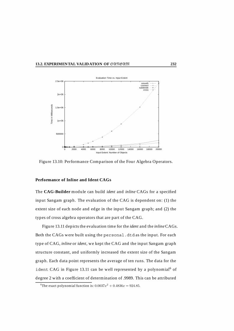
13.2. EXPERIMENTAL VALIDATION OF SANGAM 232
0
500000
1e+06
1.5e+06
2e+06
2.5e+06
0 2000 4000 6000 8000 10000 12000 14000 16000 18000 20000
Tim
e in
Mill
isec
onds
Input Extent: Number of Objects
Evaluation Time vs. Input Extent
smoothconnect
subdividecross
Figure 13.10: Performance Comparison of the Four Algebra Operators.
Performance of Inline and Ident CAGs
The CAG-Builder module can build ident and inline CAGs for a specified
input Sangam graph. The evaluation of the CAG is dependent on: (1) the
extent size of each node and edge in the input Sangam graph; and (2) the
types of cross algebra operators that are part of the CAG.
Figure 13.11 depicts the evaluation time for the ident and the inline CAGs.
Both the CAGs were built using the personal.dtd as the input. For each
type of CAG, inline or ident, we kept the CAG and the input Sangam graph
structure constant, and uniformly increased the extent size of the Sangam
graph. Each data point represents the average of ten runs. The data for the
ident CAG in Figure 13.11 can be well represented by a polynomial6 of
degree 2 with a coefficient of determination of .9989. This can be attributed6The exact polynomial function is: 0.0037x2 + 0.4836x 924.85.

13.2. EXPERIMENTAL VALIDATION OF SANGAM 233
0
200000
400000
600000
800000
1e+06
1.2e+06
0 2000 4000 6000 8000 10000 12000 14000 16000
Tim
e in
Mill
isec
onds
Input Extent: Number of Objects
Evaluation Time vs. Input Extent
inlineident
Figure 13.11: The Time Taken to Evaluate Ident and Inline CAGs as theExtent Size of the Input Sangam Graph Loaded from the personal.dtdis Varied.
to the fact that the ident CAG is comprised only of cross and connect al-
gebra operators which are Ø(n) and Ø(n2) respectively. On the other hand,
the performance of the inlineCAG which comprises of cross, connect
and smooth can be well represented by a polynomial7 of degree 3 with a
coefficient of determination of 0.9997. The dominant factor here is the per-
formance of the smooth operator which is Ø(n3).
Figure 13.12 also depicts similar results for the evaluation times of both
the ident and the inline CAGs when run with the auction.dtd as input.
7The exact polynomial function is: 5e0.08x3 + 0.0058x2 8.3567x + 1400.6.

13.2. EXPERIMENTAL VALIDATION OF SANGAM 234
0
20000
40000
60000
80000
100000
120000
140000
1 1.5 2 2.5 3 3.5 4 4.5 5
Tim
e in
Mill
isec
onds
XML Size in MegaBytes
Evaluation Time vs. XML Size
Inline CAG Evaluation TimeIdent CAG Evaluation Time
Figure 13.12: The Time Taken to Evaluate Ident and Inline CAGs as theExtent Size of the Input Sangam Graph Loaded from the auction.dtd isVaried.
13.2.3 Summary of Experimental Results
In summary, we can draw the following conclusions based on the experi-
mental results:
• the DTD loading cost, i.e., the time taken to construct a Sangam graph
from a given DTD, increases linearly with a linear increase in DTD
size;
• the XML loading cost, i.e., the time taken to load the XML documents
as the extent of the Sangam graph, increases linearly with a linear
increase in XML size;
• the evaluation times for the cross operator increase linearly with a

13.3. SUMMARY 235
linear increase in input extent size;
• the evaluation time for the connect, smooth and subdivide op-
erators can be approximated by polynomials with respect to input
extent size;
• the evaluation time for a CAG is a function of operator types and size
of the CAG;
13.3 Summary
In this chapter, we present Sangam, a prototype system that we have im-
plemented based on the theory presented in Chapters 11 and 12. We have
also presented a set of experiments that verify the feasibility of the Sangam
graph model and the cross algebra graph as presented in Chapters 11 and 7
respectively; and also measure the costs for the different components of the
system architecture (Section 13.1) used to transform one XML document to
another XML document, or to transform one XML document to a relational
database.

13.3. SUMMARY 236

237
Chapter 14
Updating the Sangam Graph
Information is not static, rather it changes over time. A Sangam Graph rep-
resents an application (data model specific) schema and its data. These two
are referred to as the local schema and local data. Any change in the local
schema and data must be reflected in the Sangam graph . To enable this
capability, we first present a taxonomy of primitive operations that can be
applied on the Sangam graph resulting in a modified Sangam graph . This
taxonomy of primitives includes operators for schema change to the Sang-
am graph (called SAG-SC, SAG-Schema Change) as well as operators for
data modification (called SAG-DU, SAG-Data Update). As a second step
we show how local schema and data changes expressed in the native data
model data manipulation and data definition language can be modeled by
a combination of SAG-SC and SAG-DU operations. Specifically we show
how XML and relational updates can be translated into a sequence of SAG-
SC and SAG-DU operations.

14.1. SCHEMA CHANGE OPERATIONS ON THE SANGAM GRAPH 238
14.1 Schema Change Operations on the Sangam Graph
14.1.1 SAG-SC: Schema Change Primitives
The insertNode Operation. Given an input Sangam graph G such that
node m 2 G, the operation insertNode (ln, τ , m, el, q), creates a new node
n1 with type τ 2 Γ and labelln, and inserts it into the input Sangam graph
G to produce a new modified Sangam graph G’ such that a new edge e
with label el and quantifier annotation q, connects the node n to the node
m, i.e., e:<m, n>. The insertNode operator appends the node n as the last
child of the node m2, i.e., the edge e:<m, n> is inserted such that the order
annotation ρ(e) = j + 1, where j = max(ρ(ei)j8 ei:<m, ni >).
To handle order-specific insertions, such as with XML schemas, we de-
fine an additional insert operation insertNodeAt (ln, τ , m, el, q, pos). The
insertNodeAt operation creates the new node n with the label ln and a
new edge e:<m, n> with order annotation of pos, i.e., ρ(e) = pos. For all
edges ei:<m,ni> 2 G such that the order annotation ρ(ei) pos, the order
annotation of ei is updated such that ρ(ei) = ρ(ei) + 1. The label and
the quantifier annotation of the edge are specified by parameters el and q
as before.
The insertNode operation fails if either (1) the label ln of the new node
n is the same as the label li of some other node ni and the nodes n and ni
share a common parent m; or (2) the type of the node n τ /2 Γ. In addition
to the above conditions the insertNodeAt fails if either (1) ρ(e) is specified
1Recall from Section 11 that a node n has a label ln and an extent denoted as I (n).2The node m maybe specified as null, in which case the node n is regarded as the root of
the Sangam graph .

14.1. SCHEMA CHANGE OPERATIONS ON THE SANGAM GRAPH 239
such that there exists no other edge e i:<m, ni> such that ρ(ei) < pos; or
(2) if pos 0;
The deleteNode Operation. Given an input Sangam graph G, the opera-
tion deleteNode (n, m) removes the node n and the edge e:<m, n> to pro-
duce a new Sangam graph G’. For all edges ei:<m,ni> with order annota-
tion ρ(ei) > ρ(e), the new order annotation of edge ei is updated such that
ρ(ei) = ρ(ei) 1. For example, if node m connects to three nodes o, n,
p with order annotations 1, 2 and 3 respectively, then the deletion of the
noden results in nodem containing two nodeso, pwith order annotations
1 and 2 respectively.
The operation fails if either (1) there is no edge e:<m, n> in G; or (2) if
the node n has other incoming edges (besides e); or (3) if it is not a leaf3,
i.e., is has other children nodes.
The insertEdge Operation. Given an input Sangam graph G, the opera-
tion insertEdge (m, n, l, q), creates a new edge e:<m, n> between the nodes
m and n, with m, n2 Sangam graph G, with label l and quantifier annotation
q. Here the order annotation ρ(e) = j + 1, where j = max(ρ(ei)j8 ei:<m,
ni>, ni 2 G). We also provide the insertEdgeAt operation, insertEdgeAt (m,
n, l, q, pos), that inserts an edge e:<m, n> with label l and quantifier
annotation q, such that the order annotation ρ(e) = pos. If there already
exists an edge ei:<m,ni> such that ρ(ei) pos, then the order annotation
of ei is updated such that ρ(ei) = ρ(ei) + 1.
3For precise definition of a leaf, please refer to Chapter 11.

14.1. SCHEMA CHANGE OPERATIONS ON THE SANGAM GRAPH 240
The insertEdge operation fails if either of the nodesn or m do not exist in
the Sangam graph G. In addition to the above condition, the insertEdgeAt
operation fails if either (1) pos is specified such that there exists no other
edge ei:<m, ni> such that ρ(ei) < pos; or (2) if pos 0.
The deleteEdge Operation. Given an input Sangam graph G, the opera-
tion deleteEdge (m,l) deletes the edge e:<m, n> with label l from node m
to node n. If there exists an edge ei:<m,ni> such that ρ(ei) > ρ(e), then the
order annotation of ei is updated such that ρ(ei) = ρ(ei) 1.
The operation fails if either (1) there is no edge e:<m,n> 2 G with label
l; or (2) if node n 2 G’ has no incoming edges, i.e., if the node n would no
longer be connected in G’.
The rename Operation. The rename operation, rename (n, l’), modifies
the label of the node n 2 G to label l’ to produce a new Sangam graph G’.
The operation fails if (1) the node n does not exist in the Sangam graph
G; (2) if the label l’ is the same as the old label l; or (2) there exists a node
ni with label l’ such that both n and ni have a common parent m in G’.
14.1.2 Completeness of SAG-SC Operations
Table 14.1 summarizes the taxonomy of change operations that we have
presented above. This taxonomy intuitively captures all changes needed
to manipulate the Sangam graph (refer Section 11). Here we outline a
proof that shows that this set indeed subsumes every possible type of graph
change (completeness criteria). The proof given here is based on the com-

14.1. SCHEMA CHANGE OPERATIONS ON THE SANGAM GRAPH 241
pleteness proof given by Banerjee et al. for the evolution taxonomy of
Orion [BKKK87].
SAG Primitive DescriptioninsertNode (ln, τ , m, l, q) Creates new node with label ln and inserts it
as child of node minsertNodeAt (ln, τ , m, l, q, pos) Creates new node with label ln and inserts it
as child of node m at position posdeleteNode (m, n) Deletes child node n from parent minsertEdge (m, n,l, q) Inserts new edge between nodes m and n,
making n child of node minsertEdgeAt (m, n,l, q, pos) Inserts new edge at position pos between
nodes m and n, making n child of node mdeleteEdge (m, l) Deletes edge e with label l from the node mrename (n, l’) Modifies label of node n to l’
Table 14.1: Taxonomy of Sangam Graph Structural Change Primitives.
In order to show completeness of these operations we prove that every
valid Sangam graph as per Definition 6 can be generated by the operations
in Section 14.1 from any other given Sangam graph .
Lemma 9 For any given Sangam graph G, there is a finite sequence of deleteNode
operations that can reduce the Sangam graph G to a Sangam graph G’ consisting
of only one single node.
Proof: It is apparent that if we repeatedly apply the operation deleteNode
to a leaf node n which removes a node n and an edge e:<m, n> from a
Sangam graph G, we can after a finite number of applications reduce any
given Sangam graph G to a new Sangam graph G’which only has one node.
Lemma 10 There is a finite sequence of operations insertNode , insertNodeAt that generates any desired Sangam graph G from an empty Sangam graph G’.

14.1. SCHEMA CHANGE OPERATIONS ON THE SANGAM GRAPH 242
Proof: Let G be a Sangam graph with a finite number of nodes and
edges and one root, and G’ be an empty. The following procedure can, via
the finite sequence of operations listed above, transform the empty Sang-
am graph G’ to any desired Sangam graph G. To achieve this, we traverse G
in a breadth-first order starting at the root node r of G and do the following:
1. Set node n r.
2. For the node n, add a corresponding node n’ to Sangam graph G’ us-
ing operation insertNodeAt (n.label, n.τ , n.parent, ne.label,
Ω(ne), ρ(ne)), where ne: <n.parent, n>. The node n’ has the same
label as n and the same type τ .
3. Traverse the set of outgoing edges from the node n and for each out-
going edge e:<n, r>, repeat steps (1), (2) and (3) for r.
The resultant Sangam graph G’ is equivalent to the initial Sangam-
graph G as they have the same set of nodes and edges but different OIDs.
2
Theorem 9 Given two arbitrary Sangam graphs G and G’, there is a finite se-
quence F of operations of type insertNode , insertNodeAt , deleteNode , such
that when F is applied to the Sangam graph G it produces the Sangam graph G’.
Proof: We can prove this by first reducing the Sangam graph G to an
intermediate Sangam graph G1 using Lemma 9. The Sangam graph G1 can
then be converted to Sangam graph G’ using Lemma 10. 2
The set of operations insertNode , insertNodeAt , deleteNode is a
subset of the operations insertNode , insertNodeAt , deleteNode , insertEdge ,
14.1. SCHEMA CHANGE OPERATIONS ON THE SANGAM GRAPH 243
insertEdgeAt , deleteEdge , rename . Hence the completeness of this set
of operations follows from Theorem 9.
14.1.3 Correctness of Sangam graph -SC Operations
We next define correctness of a SAG-SC operation as given below.
Definition 23 (Correctness) A SAG-SC operation c applied on a Sangam graph
G is correct, if when given a valid Sangam graph G its application produces as
output a Sangam graph G ’ that also is valid by Definition 6.
Theorem 10 (Correctness of SAG-SC Operations) All operations c 2 in-
sertNode , insertNodeAt , deleteNode , insertEdge , insertEdgeAt , deleteEdge ,
rename are correct.
Proof 1 Assume that the input Sangam graph is a valid Sangam graph by Defi-
nition 6. Now let us consider the deleteNode operation. We know by Definition 6,
a valid Sangam graph must be (2) connected and (3) type τ of all nodes n in G is
in Γ. As the deleteNode operation deletes a node, property (3) is not affected. In
the deleteNode operation we observe that the operation fails if the node n that is
to be deleted has any outgoing edges. This prevents the creation of un-connected
Sangam graphs . Moreover, the deleteNode operation removes the edge e from
the parent m to the child node n, such that no dangling edges without target nodes
would remain. Thus, the deleteNode operation produces a valid Sangam graph as
output when given a valid Sangam graph as input.
Next consider the insertNode operation. Given that the input Sangam graph G
is valid, an insertNode operation inserts a new node with label l and type τ . The

14.2. DATA MODIFICATION PRIMITIVES FOR THESANGAM GRAPH 244
operation insertNode fails if τ /2 Γ, ensuring that on completion of insertNode
operation, all nodes of G’ have a type τ in Γ. The insertNode operation inserts a
node n in G’ as a child of a specified parent node m, thus preventing the creation
of un-connected Sangam graphs . Moreover, the insertNode operation appends
the node as a child of the parent node. Hence the order annotation of the outgoing
edges from the parent is maintained.
A similar inspection of the other SAG-SC operations shows that they produce
valid Sangam graphs as output.
14.2 Data Modification Primitives for the
Sangam Graph
Similar to the SAG-SC operations, we now define four data modification
primitives that can insert and delete nodeObjects into and from the extent
I (n) of a node n, and insert and delete edgeObjects into the extent R (e) of
an edge e.
The addObject Operation. The addObject operation, given as addObject
(v,n), creates a new object o with data value v and inserts the object o into
the extent I (n) of node n.
The addObject operation fails if either (1) for any outgoing edge e of
node n the minimum quantifier annotation is 1, requiring that the object o
must be connected to some other object oi in the extent I (ni) of node ni,
where ni is a child of node n; or (2)for any incoming edge em:<m, n>, the
minimum quantifier annotation is 1, requiring that the object o must be

14.2. DATA MODIFICATION PRIMITIVES FOR THESANGAM GRAPH 245
connected to some other object om in the extent I (m).
The deleteObject Operation. The deleteObject operation, given as de-
leteObject (o,n), removes the object o from the extent I (n) of node n.
The operation fails if (1) there is no object o 2 I (n); (2) if there exists any
edgeObject oe: <o1, o2> in R (e) such that o1 = o or o2 = o and e is an
outgoing or an incoming edge of node n.
The renameValue Operation. The renameValue operation, given as re-
nameValue (o, v’, n), updates the value of object o 2 I (n) to the new value
v’.
The operation fails if there exists no object o 2 I (n).
The addEdgeObject Operation. The addEdgeObject operation, given as
addEdgeObject (o1,o2,e), creates a new edgeObject oe:<o1, o2> and in-
serts the edgeObject oe into the extent R (e) of edge e:<m, n>.
The operation fails if (1) o1 /2 I (m) or o2 /2 I (n); (2) there is no edge
e:<m,n>2 G; (3) the edgeObject oe:<o1,o2> already exists, i.e., oe:<o1,o2>
2 R (e); or (4) the addition of the edgeObject oe:<o1,o2> violates the max-
imum quantifier annotation of the edge e.
The deleteEdgeObject Operation. The deleteEdgeObject operation, given
as
deleteEdgeObject (oe,e), removes the object oe from the extent R (e) of
edge e:m!n.

14.3. TRANSLATION COMPLETENESS OF SANGAM GRAPHOPERATIONS 246
The operation fails if (1) oe /2 R (e); (2) the deletion of oe:<o1, o2> vio-
lates the minimum quantifier annotation of the edge e; or (3) the removal
of the edgeObject oe causes the nodeObject o2 to become dis-connected.
14.3 Translation Completeness of Sangam Graph Op-
erations
14.3.1 Translation Completeness of SAG-SC Operations
Perhaps more important than the completeness of the SAG-SC operations
shown in Section 14.1.2 is the completeness of the SAG-SC operations with
respect to local data model changes. We term this as the translation com-
pleteness. For example, if we consider the XML data model, then we call
the SAG-SC operations translation complete if all XML schema changes can
be translated into a sequence of SAG-SC operations that achieve the same
effect on the Sangam graph that represents the XML DTD. In this section,
we show that the SAG-SC operations are indeed translation complete with
respect to XML and relational schema changes.
XML Changes
To execute schema changes on XML, we use the XEM system [SKC+01].
The XEM system (XML Evolution Manager) has been developed by Hong
et al. at Worcester Polytechnic Institute is a complete XML evolution fa-
cility that provides a minimal yet complete taxonomy of XML evolution
operations. Table 14.2 enumerates the DTD operations provided by XEM.

14.3. TRANSLATION COMPLETENESS OF SANGAM GRAPHOPERATIONS 247
DTD Operation DescriptioncreateDTDEl(u) Create element with name udestroyDTDEl(u) Destroy element with name urenameDTDEl(u, u’) Rename element from name u to u’insertDTDEl(E, pos, P, q, d) Add element E at position pos to parent P with
quantifier q and default value dremoveDTDEl(E, P) Remove sub-element E in parent PchangeQuant(E, P, q, d) Change quantifier of subElement E in parent
P to quantifier qconvertToGroup(E, start, end) Group sub-elements from position start to po-
sition end in parent E into a list groupflattenGroup(E, pos) Flatten group at position pos in element E to a
list of sub-elementsaddDTDAtt(u, E, t, d, v) Add attribute with name u to element E with
type t, default type d, and default value vdestroyDTDAtt(u, E) Destroy attribute with name u from element
EchangeAttDefType(u, E, t, v) Change element E’s attribute u’s type to t,
with default value vchangeAttDefValue(u, E, v) Change element E’s attribute u’s default
value to v
Table 14.2: DTD Data Change Primitives of XEM [SKC+01].
Now consider the operation insertDTDEl(E, pos, P, q, d) that
adds element E at position pos to parent P with quantifier q and default
value d. To translate this operation into an operation(s) on the Sangam-
graph , we need to consider that4: (1) each XML element is represented by a
node in the Sangam graph . Hence, the elements E and P are represented by
Sangam graph nodes n and m respectively; (2) the parent-child relationship
is represented by an edge e between the Sangam graph nodes m and n;
(3) the quantifier q is translated into the quantifier annotation on edge e.
The rules for the quantifier translation are as given in Section 11; (4) the
order of the element e as given by the parameter pos is translated into the
4This is a summarization of the process to translate an XML DTD into a Sangam graph .For more details on this refer to Chapter 11.

14.3. TRANSLATION COMPLETENESS OF SANGAM GRAPHOPERATIONS 248
order annotation for the edge e; and (5) the default value d is a property of
element E and is represented by atomic node dv5. The nodedv is connected
to the parent noden by an edgede:<n,dv> that has a quantifier annotation
of [1:1], and order annotation of 1.
Assuming that the XML elements P and E are represented by nodes m
and n in Sangam graph G respectively, the insertDTDEl operation maps
to the sequence of the following operations. Here the operation insert-
DTDEl is inserting an element E as a subelement of the element P. The
elements E and P are already defined in the DTD. We make the same as-
sumption for the Sangam graph .
DTD Operation SAG-SC Sequence Description
createDTDEl(u)
insertNode (u, τ , D, l, q) Creates a new node n with label u andinserts it as a child of node D such thatthere is now an edge e:<D, n>. Theedge e has a label l and quantifier an-notation of q. The order annotation,ρ(e) is as calculated as specified for op-eration insertNode .
destroyDTDEl(u) deleteNode (n, D) Deletes node n with label u from parentD
renameDTDEl(u, u’) rename (n, u’) Renames the label of node n from u tou’
insertDTDEl(E, pos, P, q,d)
insertNodeAt (n.label, τ , m, l, q’, pos) Creates a new node ns with labeln.label where n is the node that rep-resents the definition of element E. Thenode ns is inserted as a child of nodem where m represents the XML elementP. The edge e:<m, ns> has a label l,quantifier annotation Ω(e) =q and anorder annotation ρ(e) = pos.
insertEdge (ns, n, l, q) Creates an edge ep :<ns , n> with labell and Ω(e) = q.
insertNode (dv, τ , ns , “default”, q) Inserts an atomic node dv as a child ofnode ns to model the default value
removeDTDEl(E, P) deleteNode (m, n) Deletes the node n, and edge e:<m, n>
Table 14.3: Translation of XEM Primitives to SAG-SC Operations.
1. insertNodeAt (n.label, τ , m, “childElement”, q’, pos). This oper-
ation creates a new node ns with the same label as the node n, and
5The default value is used when new nodeObejcts are created without a specific value.

14.3. TRANSLATION COMPLETENESS OF SANGAM GRAPHOPERATIONS 249
DTD Operation SAG-SC Sequence Description
changeQuant(E, q, q’)
insertEdge (m, n, e.label, q’) Inserts a new edge e’:<m, n> withΩ(e’) = q’. The label of e’ is the sameas label of e; and ρ(e’) = ρ(e).
deleteEdge (m, e.label) delete edge e:<m, n>.
convertToGroup(E, start,end)
insertNodeAt (ln, τ , n, l, q, start) Creates a new node g with label ln andinserts the node as a child of node n.The edge e:<n, g> is created betweenthe nodes n and g with a label l, Ω(e)= [1:1] and ρ(e) = start.
i start + 1while i 6= end + 1 :
ni nodeAt(n, i) Retrieve the node ni such that ρ(ei) =i for edge ei :<n, ni>
pos 1 Initialize the order index to 1insertEdgeAt (g, ni , ei .label,
Ω(ei), pos)Insert edge e:<g, ni> with the label,quantifier annotation and order annota-tion of the edge ei :<n, ni>
deleteEdge (n, ei.label) Delete the edge ei :<n,ni>pos++ Increment the order variable
Table 14.4: Translation of XEM Primitives to SAG-SC Operations.
DTD Operation SAG-SC Sequence Description
flattenGroup(E, pos)
g nodeAt(n, pos) Get the node g such that ρ(e) = pos,where e:<n, g>
children children(g) Get all the nodes ni such that there ex-ists an edge ei :<g, ni>
for ni in children:insertEdgeAt (n, ni , ei.label,
Ω(ei), pos)Create a new edge ei’:<n, ni> suchthat label of ei’ is the same as label ofei , Ω(ei’) = Ω(ei) and ρ(ei’) = pos.For the first node ni , ρ(ei’) = ρ(e) =pos.
deleteEdge (n, e.label) Delete the edge e:<n, g>pos++ Increment the order variable
deleteNode (n, g) Delete the node g, a child of node n
addDTDAtt(u, E, t, d, v)
insertNode (u, n, l, q) Create a node ni with label u and in-sert it as a child of node n. For this cre-ate an edge ei :<n, ni> such that eihas a label l, Ω(ei) = q and ρ(ei) isassigned based on rules defined underthe insertNode operation.
for each property p: For each XML property, (type, de-fault, defaultType) insert atomicnodes that capture the schema levelproperties of the node
insertNode (p, ni, l, q) Create a new atomic node an with labelp and insert it as a child of node ni suchthat the edge ean :<ni , an> has a la-bel l, Ω(an) = q and ρ(ean) is as perthe operation insertNode .
destroyDTDAtt(u, E) deleteNode (n, ni) Delete the node ni with label u suchthat e:<n,ni>
Table 14.5: Translation of XEM Primitives to SAG-SC Operations.
inserts the node as a child of node m. The edge e:<m, ns> has a
quantifier annotation q’, an order annotation of pos and a label of
“childElement”. The quantifier annotation q’ = [0:n] if input pa-
14.3. TRANSLATION COMPLETENESS OF SANGAM GRAPHOPERATIONS 250
rameter q of the insertDTDEl operation is “”, q’ = [1:n] for q =
“+”, q’ = [0:1] for q = “?”, and q’ = [1:1] otherwise.
2. insertEdge (ns, n, “subElement”, q). This operation inserts an edge e
from the newly created subelement ns to its definition n. This defini-
tion is given by the node n. The quantifier q for this edge e is always
set to [1:1], and the order annotation is set to 1.
3. insertNode (dv, τ , ns, “default”, q): This operation inserts a new
atomic node dv to capture the default value of the element E when
it occurs as a child of the element P. Here the τ indicates that this has
an atomic node type. An edge e:<ns,dv> is created and inserted as
an outgoing edge of n. The quantifier q for the edge e:<ns,dv> is set
to [0:1].
The above sequence of updates simulates the insertion of the element
E as a subelement of element P in an XML DTD. Tables 14.3, 14.4 and
14.5 give the synopsis of the update sequence of SAG-SC operations that
achieve the semantics of the XEM operations. Here we assume that the
Sangam graph node D represents the DTD node, the nodes m and n repre-
sent the elements P and E respectively, and unless specified otherwise τ (n)
represents a complex Sangam graph node type.
Relational Schema Changes
For the relational model we consider the set of operations provided for
schema evolution in SQL-99 [Tr00]. A set of common schema operations
for commercial database systems is given in Table 14.6.

14.3. TRANSLATION COMPLETENESS OF SANGAM GRAPHOPERATIONS 251
Evolution Primitive DescriptionCREATE TABLE Creates a new tableDROP TABLE Drops the tableALTER TABLE ADD COLUMN Adds a column to the tableALTER TABLE DROP COLUMN Drops a column of the tableALTER TABLE ALTER COLUMN<name>
Alters the column label
ALTER TABLE ALTER COLUMN SETDATA TYPE
Alters the column data type
Table 14.6: Taxonomy of Relational Schema Evolution Primitives.
Table 14.7 gives the sequence of SAG-SC operations for each of the re-
lational schema evolution operations. Here we assume that the Sangam
graph node S represents the entire relational schema, i.e., all relational ta-
bles for the schema are children of the node S (For more details please refer
to Chapter 11). All relational evolution operations are assumed to operate
within the schema S. For example, the operation CREATE TABLE t creates
a new table t in the default schema which here is assumed to be schema S.
As before τ always indicates a complex node unless specified otherwise.
14.3.2 Translation Completeness of SAG-DU Operations
Given that the goal of our work is to enable the translation of a schema
and its data in one data model to another, it is essential that similar to the
local schema changes, we are able to translate all data changes in one data
model to data changes in another data model. We show in this section
the translation completeness of the SAG-DU operations with respect to the
XML and relational data updates.

14.3. TRANSLATION COMPLETENESS OF SANGAM GRAPHOPERATIONS 252
Relational Primitive SAG-SC Operations DescriptionCREATE TABLE t insertNode (t, τ , S,
l, q)Creates a node n with labelt. It inserts the node n as achild of the node S such thate:<S, n>. The edge e has alabel l and Ω(q) = q. Hereq = [1:1]. The order anno-tation ρ(e) is assigned by thesystem as per the definitionof the insertNode operation.
DROP TABLE t deleteNode (n, S) Deletes the node nwith labelt.
ALTER TABLE t ADDCOLUMN c
insertNode (c, τ , n,l, q)
Adds a node ni with labelc. It inserts the node ni asa child of node n such thatthere is an edge e:<n, ni>with label l, Ω(e) = q. Hereq = [0:1], if attribute canbe NULL or q = [1:1] ifattribute is NOT NULL. Theorder annotation ρ(e) is as-signed by the system as perthe definition of insertNodeoperation.
ALTER TABLE t DROPCOLUMN c
deleteNode (n, ni) Deletes the node ni with la-bel c from the parent node n.
ALTER TABLE tALTERCOLUMN c <name>
rename (ni, l’) Modifies the label of thenode ni from c to l’.
ALTER TABLE tALTERCOLUMN c SET DATATYPE ty
rename (dt, ty’) Modifies the label of nodedt that is a child node of thenode ni with label c to ty’.
Table 14.7: Translation of Relational Schema Evolution Primitives to SAG-SC Operations.
Translating XML Data Updates
We assume that all changes to XML documents are made via the the XML
update primitives proposed by Tatarinov et al. [TIHW01]. Table 14.86 gives6They do not make the separation between the value and the child in their work.
Rather they are both part of the syntactical extension they propose for Quilt (XQuery). To
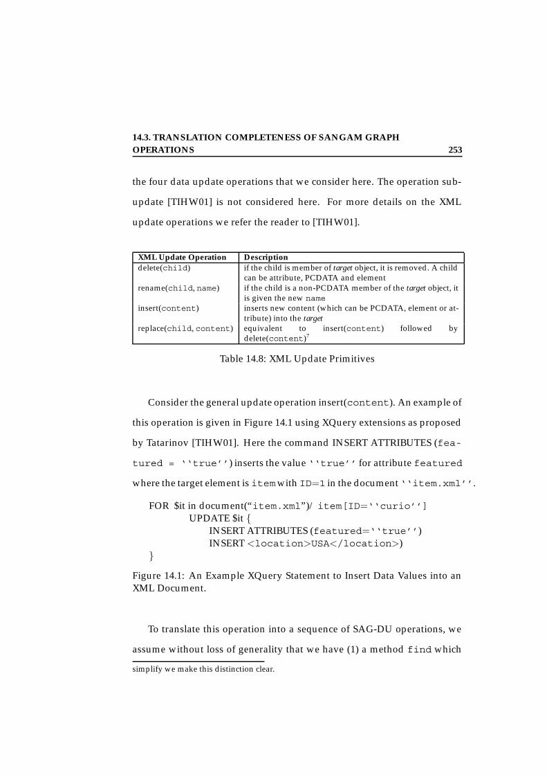
14.3. TRANSLATION COMPLETENESS OF SANGAM GRAPHOPERATIONS 253
the four data update operations that we consider here. The operation sub-
update [TIHW01] is not considered here. For more details on the XML
update operations we refer the reader to [TIHW01].
XML Update Operation Descriptiondelete(child) if the child is member of target object, it is removed. A child
can be attribute, PCDATA and elementrename(child, name) if the child is a non-PCDATA member of the target object, it
is given the new nameinsert(content) inserts new content (which can be PCDATA, element or at-
tribute) into the targetreplace(child, content) equivalent to insert(content) followed by
delete(content)7
Table 14.8: XML Update Primitives
Consider the general update operation insert(content). An example of
this operation is given in Figure 14.1 using XQuery extensions as proposed
by Tatarinov [TIHW01]. Here the command INSERT ATTRIBUTES (fea-
tured = ‘‘true’’) inserts the value ‘‘true’’ for attribute featured
where the target element is itemwith ID=1 in the document‘‘item.xml’’.
FOR $it in document(“item.xml”)/ item[ID=‘‘curio’’]UPDATE $it
INSERT ATTRIBUTES (featured=‘‘true’’)INSERT <location>USA</location>)
Figure 14.1: An Example XQuery Statement to Insert Data Values into anXML Document.
To translate this operation into a sequence of SAG-DU operations, we
assume without loss of generality that we have (1) a method find which
simplify we make this distinction clear.

14.3. TRANSLATION COMPLETENESS OF SANGAM GRAPHOPERATIONS 254
returns the Sangam graph node representing a given schema entity label;
(2) a method getNodeObject(I (n), v) that returns the set of nodeOb-
jects oi 2 I (n) that have a value v; and (3) method getEdgeObject(R
(e), oi) that returns the edgeObjects oe:<o1, o2> 2 R (e) when either o1
= oi or o2 = oi. To simplify the syntax used for the example, let the target
item be represented by node m, the ID by node n, the attribute featured
by node p, the edge mn:<item,ID> and the edge mn:<item,featured>
in the Sangam graph that represents the XML schema (see Figure 11.3). The
operation INSERT ATTRIBUTES (featured = ‘‘true’’) is translated
to the following sequence of SAG-DU operations. Here we use the XQuery
as shown in Figure 14.1 to provide the context/input parameters that may
be needed for the translation to SAG-DU operations.
1. addObject (‘‘true’’,p): Creates a new object owith value ‘‘true’’
and inserts it into I (p). Recall that here node p represents the XML
attribute featured.
2. The query in Figure 14.1 performs an update to the element item
with ID = ‘‘curio’’. We assume here that the Sangam graph is
materialized, and all item and ID objects have been created, trans-
lated from the XML document and inserted into the extents of nodes
m and n in the Sangam graph respectively, as per the algorithms given
in Section 11. Let oe getEdgeObject(R (mn), getNodeObject(I
(n),curio) return the edgeObject oe:<o1, o2> that links an object o1
of node item to an object o2 of node ID such that the value of o2 =
curio.

14.3. TRANSLATION COMPLETENESS OF SANGAM GRAPHOPERATIONS 255
3. addEdgeObject (o1, o, mp): Creates a new edgeObject oe2:<o1, o>
and inserts it into the extent R (mn) of edge mp:<m, p>, where m rep-
resents the XML element item and p the XML attribute featured.
The result of the above sequence of steps is the creation of a new object
that represents the statement featured = ‘‘true’’ that is now linked
to the correct item object. Let r denote the Sangam graph node that repre-
sents the XML Element location, and the edge mr:<m, r> that represents
the edge between the parent XML element item and the child element
location. The command INSERT (<location>USA</location>)
can then be translated to a sequence of SGM-DU operations as follows.
Here we use the tag names in the query to find the right node into which
the value is inserted.
1. addObject (‘‘USA’’,r): Creates a new object or with value ‘‘USA’’
and inserts it into I (r).
2. As the query in Figure 14.1 performs an update to the element item
with ID = ‘‘curio’’, we again find the right object oi 2 I (m) that
is in relationship with the object or. This is the same as Step 2 above.
3. addEdgeObject (o1, or, mr): Creates a new edgeObject oe3:<o1, or>
and inserts it into the extent R (mr) of edge mr:<m, r>, where m rep-
resents the XML element item and r the XML element location.
In general, we translate theinsert operations given as insert(content)
[TIHW01] to a pair of addObject and addEdgeObject operations for every
level of nesting. The

14.3. TRANSLATION COMPLETENESS OF SANGAM GRAPHOPERATIONS 256
INSERT ATTRIBUTES (featured=‘‘true’’) operation has one level of
nesting and hence often is translated to one pair of addObject and add-
EdgeObject functions. The INSERT
(<location>USA</location>) operation also has one level of nesting
and hence is translated to a pair of addObject and addEdgeObject opera-
tions.
Table 14.9 summarizes the translation of the XML data change primi-
tives given in Figure 14.8 into SAG-DU operations. We assume that these
methods are embedded in an XQuery statement that provides the context
for these operations. For the Table 14.9 let m and n be Sangam graph nodes
that represent XML elements and/or attribute. Let there be an edge mn:<m,
n>. Assume that oc 2 I (n) is a nodeObject such that child is the value of
oc. Let op be a nodeObject such that op 2 I (m) and op has a value parent.
Translating Relational Data Updates
For the relational data updates we consider the updates: add-tuple, de-
lete-tupleand modify-tuple. Consider that we have a table ITEM(ID
NUMBER(4), featured VARCHAR(40)). The Sangam graph G repre-
senting this schema will have a node m that represents the relation ITEM,
nodes i and f that represent the ID and featured columns. The edges
e1 and e2 represent the edge between ITEM and ID, and the edge between
ITEM and featured respectively. The add-tuple data update operation
given as add-tuple (“curio”, “true”) for the table ITEM is translated as
follows:

14.3. TRANSLATION COMPLETENESS OF SANGAM GRAPHOPERATIONS 257
XML Update Operation SAG-DU Sequence Description
delete(child)
deleteEdgeObject (oe, e) Based on the above as-sumption, first find theedgeObject oe:<op, oc>2 R (e) (provided by theXQuery context). Deletethe edgeObject oe.
deleteObject (oc, n) Delete the object oc withvalue child from the ex-tent I (n) of node n
rename(child, name)
renameValue (oc, name, n) Renames the value childto name for object oc 2 I(n). The OID of the objectremains the same
insert(content)
addObject (content, n) Creates a new object oc
with value content.Adds new object oc to I(n)8
addEdgeObject (o1, oc, e) If e represents the edgebetween the parent andthe child nodes, then cre-ate new edgeObjects andadd them to R (e).
Table 14.9: Translation of XML Update Operations to SAG-DU Operations.
1. Create a new nodeObject o1 and insert into I (m) to represent a new
row in the relational table.
2. Create a new nodeObject o2 with value ‘‘curio’’. Insert this
value into I (i).
3. Create a new edgeObjectoe1:<o1, o2> to represent the relationship
between the object o1 and o2. Insert this object into R (e1).
4. Create a new nodeObject o3 with value ‘‘true’’. Insert this
value into I (f).
5. Create a new edgeObjectoe2:<o1, o3> to represent the relationship

14.3. TRANSLATION COMPLETENESS OF SANGAM GRAPHOPERATIONS 258
SAG Primitive XEM Primitive Description
insertNode (ln, τ ,m, l, q)
createDTDEl(ln) If m represents the DTD node.insertDTDEl(ln, ρ(e),m.label, q, d.label)
If n represents an element. Heree is an edge such that e:<m, n>.The node d represents a prop-erty node of the n.
addDTDAtt(ln, m.label,t.label, d.label,v.label)
If node n represents an at-tribute. Here t, d, and v areproperty nodes that are chil-dren of node n. They may beempty.
insertNodeAt (ln,τ , m, l, q, pos)
insertDTDEl(ln, pos,m.label, q, d.label)
If n represents an element
addDTDAtt(ln, m.label,t.label, d.label,v.label)
If node n represents an at-tribute. Order and Quantifierannotations are not used in thetranslation here.
deleteNode (m, n)
destroyDTDEl(n.label) If m is the DTD node.removeDTDEl(n.label,m.label)
If n is an element.
destroyDTDAtt(n.label,m.label)
If n is an attribute.
insertEdge (m,n,l, q)
insertDTDEl(n.label,ρ(e), m.label, q,d.label)
If n is an element
addDTDAtt(n.label,m.label, t.label,d.label, v.label)
If node n represents an at-tribute.
insertEdgeAt (m,n, l, q, pos)
insertDTDEl(n.label,pos, m.label, q,d.label)
If n is an element
addDTDAtt(n.label,m.label, t.label,d.label, v.label)
If node n represents an at-tribute.
deleteEdge (m, l)
removeDTDEl(n.label,m.label)
If n is an element.
destroyDTDAtt(n.label,m.label)
If n is an attribute.
rename (n, l’) renameDTDEl(n.label, l’) if n is an element.
Table 14.10: Translation of Sangam graph Structural Change Primitives toXML Change Primitives.

14.4. REVERSING THE PROCESS 259
between the object o1 and o3. Insert this object into R (e2).
Similarly, the delete-tuple operation is translated to a sequence of
deleteEdgeObject and deleteObject SAG-DU operations; and a modify-
-tuple operation into a renameValue operation. No edgeObject modifi-
cations are needed in this case as the OIDs of the objects do not change, just
the values.
14.4 Reversing the Process
So far we have considered how local schema and data changes, i.e., changes
in a relational schema or an XML DTD, can be translated into a sequence of
Sangam graph operations. By necessity this translation must be reversable,
i.e., we must be able to translate Sangam graph operations into a relational
or XML operations. This reverse translation is simpler as it now deals with
a simpler, perhaps more primitive set of changes. Recall from Chapter 11,
that we use the leaf criteria to distinguish between an element and an at-
tribute in the XML model and between a table and an attribute in the re-
lational model. Thus, a leaf Sangam graph node (a node with no children)
is an XML subelement if it has an edge that points to a node that gives its
definition (a backpointer edge). It is an XML attribute otherwise. Similarly,
a leaf node is always a relational attribute, while a non-leaf node is a table
in the relational model. Based on this distinction, in Tables 14.10 and 14.11
we give the translation of the SAG-SC operations to XML and relational
changes respectively.
Similar to the translation of the SAG-SC operations, the SAG-DU oper-
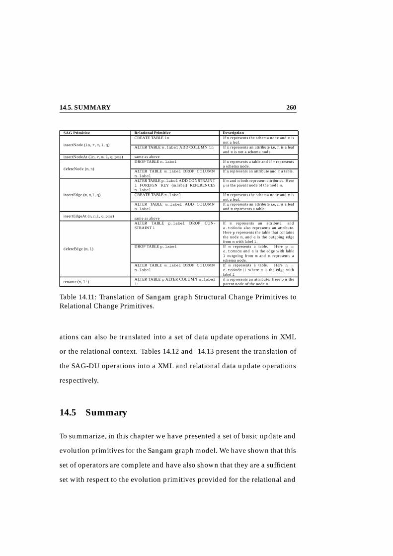
14.5. SUMMARY 260
SAG Primitive Relational Primitive Description
insertNode (ln, τ , m, l, q)
CREATE TABLE ln If m represents the schema node and n isnot a leaf.
ALTER TABLE m.label ADD COLUMN ln If n represents an attribute i.e, n is a leafand m is not a schema node.
insertNodeAt (ln, τ , m, l, q, pos) same as above
deleteNode (m, n)
DROP TABLE n.label If n represents a table and if m representsa schema node.
ALTER TABLE m.label DROP COLUMNn.label
If n represents an attribute and m a table.
insertEdge (m, n,l, q)
ALTER TABLE p.labelADD CONSTRAINTl FOREIGN KEY (m.label) REFERENCESn.label
If m and n both represent attributes. Herep is the parent node of the node m.
CREATE TABLE n.label If m represents the schema node and n isnot a leaf.
ALTER TABLE m.label ADD COLUMNn.label
If n represents an attribute i.e, n is a leafand m represents a table.
insertEdgeAt (m, n,l, q, pos) same as above
deleteEdge (m, l)
ALTER TABLE p.label DROP CON-STRAINT l
If m represents an attribute, ande.toNode also represents an attribute.Here p represents the table that containsthe node m, and e is the outgoing edgefrom m with label l.
DROP TABLE p.label If m represents a table. Here p =e.toNode and e is the edge with lablel outgoing from m and m represents aschema node.
ALTER TABLE m.label DROP COLUMNn.label
If m represents a table. Here n =e.toNode() where e is the edge withlabel l
rename (n, l’) ALTER TABLE p ALTER COLUMN n.labell’
if n represents an attribute. Here p is theparent node of the node n.
Table 14.11: Translation of Sangam graph Structural Change Primitives toRelational Change Primitives.
ations can also be translated into a set of data update operations in XML
or the relational context. Tables 14.12 and 14.13 present the translation of
the SAG-DU operations into a XML and relational data update operations
respectively.
14.5 Summary
To summarize, in this chapter we have presented a set of basic update and
evolution primitives for the Sangam graph model. We have shown that this
set of operators are complete and have also shown that they are a sufficient
set with respect to the evolution primitives provided for the relational and

14.5. SUMMARY 261
SAG DU Primitive XML DU Primitive Description
addObject (v, n) insert(v) inserts the value v into the real-world repre-sentation of n
deleteObject (o, n) delete(o.value()) Delete the value o.value from the entityrepresented by n.
rename (o, v’, n) rename ((o.value()), v’) Rename the value o.value to v’ of the en-tity represented by n.
addEdgeObject (o1, o, e)insert(content) Insert the value o.value into the entity rep-
resented by e.toNode such that its parentvalue is o1.value.
deleteEdgeObject (eo, e)delete(eo.toObject.value) Delete the value eo.toObject.value from
the entity represented by n.toNode such thatits parent value is eo.fromObject.value.
Table 14.12: Translation of Sangam graph Data Change Primitives to XMLData Change Primitives.
SAG DU Primitive Relational DU Primitive Description
addObject (v, n) add-tuple v inserts the value v into the real-world repre-sentation of n
deleteObject (o, n) delete-tuple (o.value) Delete the value o.value from the entityrepresented by n.
rename (o, v’, n) modify-tuple((o.value()), v’) Rename the value o.value to v’ of the en-tity represented by n.
addEdgeObject (o1, o, e)add-tuple (o1.value, o.value) Insert the value o.value into the entity rep-
resented by e.toNode such that its parentvalue is o1.value.
deleteEdgeObject (eo, e)
delete-tuple (eo.fromObject.value,eo.toObject.value)
Delete the value eo.fromObject.valuefrom the entity represented bye.toNode such that its parent value iseo.fromObject.value.
Table 14.13: Translation of Sangam graph Data Change Primitives to Rela-tional Data Change Primitives.
XML models. That is, we have shown that all update and evolution prim-
itives defined for the relational and XML models can be translated into a
sequence of Sangam graph primitives, to produce the a change equivalent
to the local change on the Sangam graph.

14.5. SUMMARY 262

263
Chapter 15
Update Propagation
In Chapter 14, we present a taxonomy of Sangam graph primitives using
that can be used to translate local schema and data changes into changes
on the Sangam graph . However when a Sangam graph is mapped to an-
other Sangam graph via a cross algebra graph, then to maintain consistency
between the input Sangam graph and the derived output Sangam graph
changes in the input Sangam graph must be reflected in the output Sang-
am graph . There are two possibilities for reflecting the change on the out-
put Sangam graph . The first, direct propagation, reflects any change in the
input on the output as well. The second, transparent propagation, hides when
possible, from the output any change that is made on the input. While
both mechanisms are achievable, in this dissertation we focus only on di-
rect propagation.
In this chapter, we present the direct update propagation strategy for
the cross algebra graph. For this, we first describe the overall propagation
strategy for the cross algebra graph.
15.1. THE CAT PROPAGATION STRATEGY 264
15.1 The CAT Propagation Strategy
15.1.1 Introduction
As presented in Chapter 12, the cross algebra graph consists of either con-
text dependency or derivation trees or a composition of context depen-
dency and derivation trees. Thus CAGs can be composed as a forest of one
or more context dependency and derivation trees. This follows from the
definition of the CAG (Definition 19). The propagation of a change through
a CAG can thus be achieved by the propagation of this change through each
individual tree (context dependency or derivation tree). In the forthcoming
discussion, we focus only on the propagation strategy for the CAT. The only
caveat when considering the CAT propagation is the propagation seman-
tics for a change through a shared operator (Definition 16). We address this
caveat as a separate point beyond the general propagation algorithms.
15.1.2 Updates on CAT
We now define a valid update on a Sangam graph .
Definition 24 (Valid Update) Let SC denote the set of all operations on a Sang-
am graph as defined in Section 14. An operation c 2 SC on a node n or an edge e is
defined for the SAG G if n (or e) either exists and/or is reachable by the specified
path (for delete operations) or does not exist and/or is not reachable by the specified
path (for add operations).
As shown in Section 14.3, a local schema change, i.e., a change on the
XML DTD or a relational schema, often results in a sequence of changes on
15.1. THE CAT PROPAGATION STRATEGY 265
the SAG. To meet our primary goal of propagating a local schema change
from the input Sangam graph to the output Sangam graph and hence even-
tually to the output application schema, we must thus consider the propa-
gation of a sequence of changes through the cross algebra tree. We define a
valid update sequence as follows.
Definition 25 (Valid Update Sequence) A sequence u1, u2, . . . ui . . . un (1 <
i n) with ui 2 SC , denoted by δG , is valid for Sangam graph G if ui is defined
for the Sangam graph G i1 that was obtained by applying u1, u2, . . . ui1 to G .
15.1.3 Overall Propagation Strategy
For SQL views, many incremental update strategies have been proposed
[Kel82, GB95]. Their essential focus is the calculation of the extent differ-
ence between the old V and new view V’ by adding or subtracting tuples
from the extent of the view V. In these works, the schemas of V and V’
were assumed to stay the same. In the scenario when schema changes are
considered [KR02] as in update propagation through SchemaSQL views by
Koeller et al., the changes are made in-place on the individual algebra op-
erators in the algebra tree. That is, the structure of the algebra tree remains
the same and no algebra nodes are added or deleted.
However, when propagating schema changes through a CAT not only
is the old output Sangam graph G different from the modified output Sang-
am graph G’ , but also the structure of the CAT itself may be affected. New
algebra nodes may be added as a result of an insertion and/or existing alge-
bra nodes may be removed as a result of a deletion. We find that although
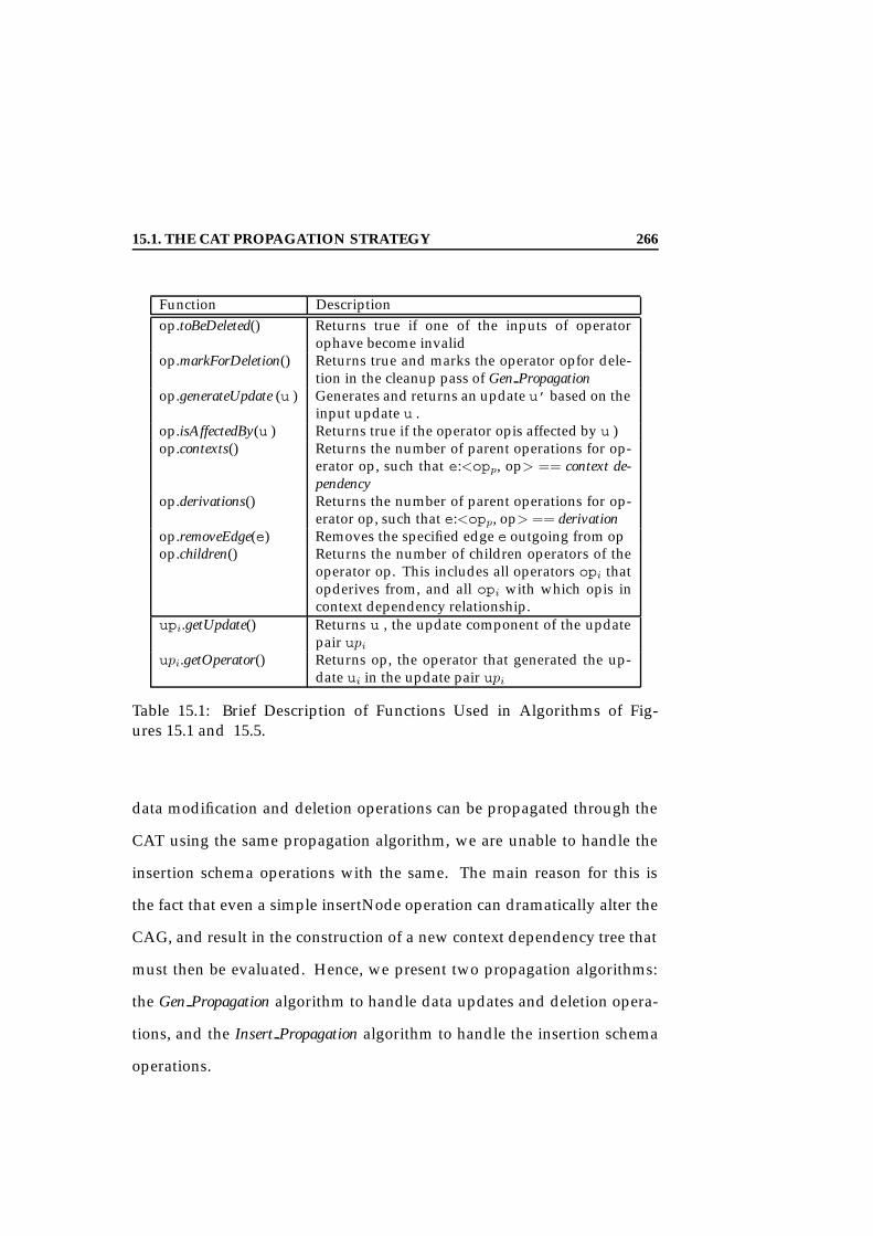
15.1. THE CAT PROPAGATION STRATEGY 266
Function Descriptionop.toBeDeleted() Returns true if one of the inputs of operator
ophave become invalidop.markForDeletion() Returns true and marks the operator opfor dele-
tion in the cleanup pass of Gen Propagationop.generateUpdate (u ) Generates and returns an update u’ based on the
input update u .op.isAffectedBy(u ) Returns true if the operator opis affected by u )op.contexts() Returns the number of parent operations for op-
erator op, such that e:<opp, op> == context de-pendency
op.derivations() Returns the number of parent operations for op-erator op, such that e:<opp, op> == derivation
op.removeEdge(e) Removes the specified edge e outgoing from opop.children() Returns the number of children operators of the
operator op. This includes all operators opi thatopderives from, and all opi with which opis incontext dependency relationship.
upi.getUpdate() Returns u , the update component of the updatepair upi
upi.getOperator() Returns op, the operator that generated the up-date ui in the update pair upi
Table 15.1: Brief Description of Functions Used in Algorithms of Fig-ures 15.1 and 15.5.
data modification and deletion operations can be propagated through the
CAT using the same propagation algorithm, we are unable to handle the
insertion schema operations with the same. The main reason for this is
the fact that even a simple insertNode operation can dramatically alter the
CAG, and result in the construction of a new context dependency tree that
must then be evaluated. Hence, we present two propagation algorithms:
the Gen Propagation algorithm to handle data updates and deletion opera-
tions, and the Insert Propagation algorithm to handle the insertion schema
operations.

15.1. THE CAT PROPAGATION STRATEGY 267
The Gen Propagation Algorithm
function List Gen Propagation (Update up , Operator opp) List inSequence ∅,
List δ ∅, //Used to gather the updates from childrenList δ’ ∅ // Represents the updates sequence of the parentUpdatePair up , upi
Boolean updateAppliedif (opp is leaf)
up applyUpdate (up , opp)δ.append (up )
else//If not a leaf, then recursively invoke Gen Propagation for all childrenfor (all children opi of opp)
δ.append(Gen Propagation (up , opi))// δ denotes all updates generated by all children of opp// Calculate the affect of each update ui 2 δ on op// Generate the parent’s update sequence δ’for (all updatePairs upi2 δ)
ui upi.getUpdate()upi’ applyUpdate (ui ,opp)//Decide if upiand upi’ must be//appended to parent’s sequence δ’ of if upimust be discardedopi upi.getOperator()if ((e:<op,opi) == contextDependency)
// Calculate effect of the original update// Check if update has been applied beforeif (!updateApplied)
up applyUpdate (up , opp)updateApplied true
δ’.append(upi)δ’.append(up )δ’.append(upi’ )
elseif ((e:<op, opi>) == derivation)δ’.append(upi’ )
return δ’;
Figure 15.1: First Pass of Cross Algebra Tree Target Maintenance Algo-rithm.

15.1. THE CAT PROPAGATION STRATEGY 268
The First Pass: Propagating the Update. The Gen Propagation algorithm
works as a two-step process. The first pass of the algorithm performs a
post-order traversal of the algebra tree. This ensures that each operator pro-
cesses the input updates after all its children have already computed their
output. Since the cross algebra tree is connected and cycle-free (Lemma 7),
all operators will be visited exactly once. If an operator is shared, then it
will contribute an update, if applicable, to all its parent operators. If the
shared operator contributes directly to the final output Sangam graph G’,
then the evaluation semantics for shared operators (Definition 16) are appli-
cable for the propagation of change, i.e., only one update will be recorded
in the final update sequence.
We can assume here without any loss of generality that each tree has
its copy of each shared operator. After all operators have been visited, the
output of the algorithm will be an update sequence δ to be applied to the
output Sangam graph G’ after the completion of the second pass.
function UpdatePair applyUpdate (Update up , Operator opp) if (opp.isAffectedBy(up ))
up’ opp.generateUpdate (up )if (opp.toBeDeleted())
opp.markForDeletion()up (up’ ,opp)
return up
Figure 15.2: First Pass of Cross Algebra Tree Target Maintenance Algorithm- The UpdatePair Function.
Figure 15.1 depicts the first pass of the Gen Propagation algorithm. Ta-
ble 15.1 lists the functions and their brief descriptions as used in Figure 15.1.
15.1. THE CAT PROPAGATION STRATEGY 269
Here, each node in the algebra tree is aware of the algebra operator it repre-
sents (see Section 7 for algebra operators). At any given time, an operator
opi can accept one input update ui, where ui 2 SC , and will generate as
output one update ui’ to be applied on the output Sangam graph G’ . The
output update for each operator is recorded as a pair <ui’, opi> in a local
update sequence δ, where ui’ is the output update and opi is the operator
to which the input update ui was applied to produce ui’. The updates ui
and ui’ are Sangam graph operation (Section 14) and are specified with all
their parameters. We assume that given an update operation, an algebra
operator can detect whether or not it is affected by the change. If it is not
affected, it will simply return the input update ui as its output.
After all the updatesui for the children of an operatoropp are computed
and collected in a sequence (denoted by variable δ in the algorithm), each
update ui 2 δ is propagated through opp, irrespective of if the child opi is
related to opp via derivation; or if child opi is related to opp via context de-
pendency. In either case, a new update ui’ will be produced by the parent
operator opp if the operator opp is effected by the update ui produced by
the child operator opi. This update ui’ is recorded as an update pair (ui’,
opp) and is appended to the update sequence δ’ produced by the operator
opp.
The edge, context dependency or derivation, between the parent and
the child operator affects the parent operator in two ways: (1) in deciding
whether the original update u must be applied to the parent operator opp;
and (2) in deciding whether the update sequence generated by the child
operator must be propagated up, i.e., included in the update sequence gen-

15.1. THE CAT PROPAGATION STRATEGY 270
erated by the parent operator.
In general, a parent operator opp is not affected by the original update u
if none of its children are affected by the same update u and all the children
are related to the parent operator by derivation. If however, the parent is
related to a child operator by a context dependency edge, then the parent
may be affected by the update u even if the child operator is not affected.
Hence, if a parent has a context dependency edge to its child operator, then
the original update u must be applied to the parent operator opp. If the
operator opp is affected by the update u, then a new update u’ and a corre-
sponding update pair up’ are generated. The update pair up’ is appended
to the update sequence δ’ produced by opp. The original update u is ap-
plied only once. The original update is not appended into the output up-
date sequence δ’ generated by an operator, but is stored as a global update.
This propagation of the update u is indicated by the following lines in the
Gen Propagation algorithm given in Figure 15.1:
// Calculate effect of the original update
up applyUpdate (up , opp)
We next consider the effect of the type of edge that exists between op p
and opi on the generation of the update sequence δ’ produced by the parent
operator opp. Recall from Chapter 12 that in a derivation tree only the out-
put of the root operator is visible in the final output produced by the tree.
It therefore follows that if there exists a derivation relationship between
opp and opi, only the update ui’ generated by opp will appear in the up-
date sequence δ’ generated by opp. Hence, after producing the update ui’,

15.1. THE CAT PROPAGATION STRATEGY 271
the update pair (ui, opi) is discarded, and the update pair (ui’, opp) is ap-
pended to the update sequence δ’1 generated by the parent operator opp.
This is given by: δ’.append(upi’ ) in the Gen Propagation algorithm depicted
in Figure 15.1. On the other hand, in a context dependency tree the outputs
of all children operators and the root operator appear in the final output
produced by the tree. Thus, if there exists a context dependency edge be-
tween the parent operator opp and the child operator opi, then the update
pair (ui, opi) is appended to the update sequence δ’ produced by the par-
ent operator opp. To maintain the dependency between the parent and the
child operator, the update pair (ui’, opp) is appended after the update pair
(ui, opi) in the update sequence δ’. This is given by the pair of statements:
δ’.append(upi’ ), δ’.append(upi), in the Gen Propagation algorithm depicted
in Figure 15.1.
For any operator opi if the update ui is such that it removes the in-
put of the operator opi, then the operator opi is marked for deletion. The
actual removal of the operator from the CAG occurs in the second pass,
Gen CleanUp , of the Gen Propagation algorithm.
The Second Pass: Cleaning Up. The purpose of the second pass is to
clean up the cross algebra tree and to ensure that the output Sangam graph
G’ after the application of δ’, the update sequence produced by pass 1, and
the clean-up still produces a valid Sangam graph . In this clean-up process,
we make the decision that:
1. if a parent operator opp that has a derivation edge to a child operator1Initially the update sequence δ’ is empty.

15.1. THE CAT PROPAGATION STRATEGY 272
opi is removed, then if the child operator opi is not a shared operator,
then opi is also removed. This follows from the fact that (1) the out-
put of a child operator is not directly visible in the output produced
by the parent operator; and (2) we do not allow partial derivation re-
sults to be reflected in the output Sangam graph G’. As an example,
consider the derivation tree DT depicted in Figure 15.3 and given by
the expression:
Figure 15.3: A Cross Algebra Graph.
DT = (op6e0:<A0,E0>(CT1, CT2)) (15.1)
where CT1 and CT2 are given as:

15.1. THE CAT PROPAGATION STRATEGY 273
CT1 = (op4eTemp1:<A0,C0>(e1 :< A, B >, e2 :< B, C >), (op1A0(A)Æop2C0(C)))
(15.2)
CT2 = (op5eTemp2:<C0 ,E0>(e3 :< C, D >, e4 :< D, E >), (op2C0(C)Æop3E0(E))).
(15.3)
Here the output produced by DT is the output of the root operator
op6, e’:<A’, E’>. The outputs of the context dependency graphs
CT1 and CT2do not appear in the final output Sangam graph . Hence,
in general it follows that if the root operator opr of a derivation tree
DT is removed, then all its non-shared children operators opi (includ-
ing the operators that are part of the the context dependency trees
CT1 and CT2) must also be removed as their output is not visible in
the final output G’. Figure 15.4 depicts the CAG after this step.
2. if a parent operator opp is removed such that there exists a context
dependency edge between the parent opp and the child opi, then the
child operator opi is not affected. This follows from the fact that in
a context dependency tree CT the outputs of all operators appear in
the final output of the tree. In the example CAG given in Figure 15.3,
the updated context dependency tree CT3 will be as depicted in Fig-
ure 15.4.

15.1. THE CAT PROPAGATION STRATEGY 274
Figure 15.4: The Updated Cross Algebra Graph After Step 1.
Figure 15.5 gives the second pass of the Gen Propagation algorithm called
Gen CleanUp . The algebra tree is traversed in in-order as the deletion
of a parent operator may affect the child operator. In the second pass
Gen CleanUp , for each operator opp marked for deletion in the first pass
Gen Propagation , if the operator opp has children operators opi connected
via derivation, then all non-shared operators opi are also marked for dele-
tion. If the operator opi is shared, then the derivation edge between opp
and opi is marked for deletion. If the operator opp has children operators
opi connected via context dependency, then the children operators op i re-
main unaffected. Once all children of an operator are visited and marked
for deletion where appropriate, all children (and edges) marked for dele-
tion are removed as well as the parent (if marked for deletion). The final
update sequence δ’ is then applied to the output Sangam graph G’.
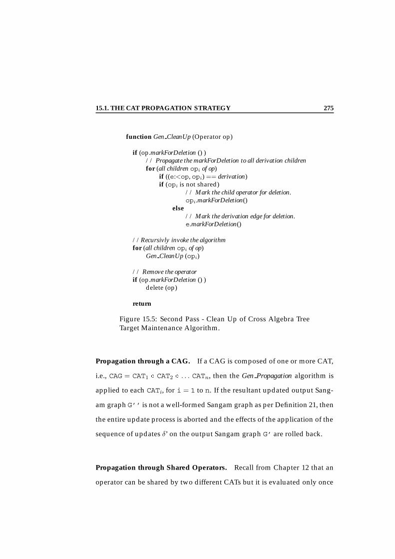
15.1. THE CAT PROPAGATION STRATEGY 275
function Gen CleanUp (Operator op)
if (op.markForDeletion () )// Propagate the markForDeletion to all derivation childrenfor (all children opi of op)
if ((e:<op, opi) == derivation)if (opi is not shared)
// Mark the child operator for deletion.opi.markForDeletion()
else// Mark the derivation edge for deletion.e.markForDeletion()
//Recursivly invoke the algorithmfor (all children opi of op)
Gen CleanUp (opi)
// Remove the operatorif (op.markForDeletion () )
delete (op)
return
Figure 15.5: Second Pass - Clean Up of Cross Algebra TreeTarget Maintenance Algorithm.
Propagation through a CAG. If a CAG is composed of one or more CAT,
i.e., CAG = CAT1 Æ CAT2 Æ . . . CATn, then the Gen Propagation algorithm is
applied to each CATi, for i = 1 to n. If the resultant updated output Sang-
am graph G’’ is not a well-formed Sangam graph as per Definition 21, then
the entire update process is aborted and the effects of the application of the
sequence of updates δ’ on the output Sangam graph G’ are rolled back.
Propagation through Shared Operators. Recall from Chapter 12 that an
operator can be shared by two different CATs but it is evaluated only once
15.1. THE CAT PROPAGATION STRATEGY 276
and hence its output directly appears at most one time in the output Sang-
am graph G’. If however a shared operator is affected by a change then the
change must be propagated through it as well as all the parent operators
to which it is linked either via a derivation or a context dependency edge.
The update produced by the shared operator appears only once in the final
update sequence δ’. This can be easily ensured by checking all the update
pairs in the final update sequence δ’.
The Insert Propagation Algorithm
The propagation of the insertNode , insertNodeAt , insertEdge , and in-
sertEdgeAt operations through the CAT to the output Sangam graph G’
is treated differently than the propagation of all other schema and data
update operations. This is mostly due to the nature of these operations and
their mapping via the cross algebra operators to the output Sangam graph
.
The insertNode and insertNodeAt Operations. Consider the CAG de-
picted in Figure 15.6 and given by the expression:
CAG = (CT1 Æ CT2) (15.4)
where CT1 = op3(e10)(e1), (op1A0(A) Æ op2B0(B))
CT2 = op5(e20)(e2, e5), (op1A0(A) Æ op4C0(C))

15.1. THE CAT PROPAGATION STRATEGY 277
Figure 15.6: An Example CAG.
Now consider that the operation insertNode (D, τ , A, el, 1:1), where D
is the label of the new node that is to be inserted into the Sangam graph G,
and el is the label of the edge e:<A, D>2. The resultant Sangam graph Gu,
after the application of the insertNode operation, is shown in Figure 15.7.
The insertNode operation creates a node as well as an edge. Given that
we employ the semantics that all changes in the input must be visible in
the output, to propagate this insertNode operation to the derived output
Sangam graph G’, we must now map the newly created node D and the
corresponding edge e:<A,D> to the output Sangam graph G’. For this we
would need to:
1. Given a CAG, find the cross algebra operator op1 that maps the node
A to produce the output A’ 2 G’. If no such operator exists in the
CAG, then a new cross operator is created such that it maps A to A’
2 G’;
2To make it easier to read, we use the labels of nodes here to refer to the actual nodeobjects.

15.1. THE CAT PROPAGATION STRATEGY 278
2. create a new cross operator op6 that maps the node D to D’ 2 G’; and
3. create a connect operator op7 that ensures that the objects of A’
will provide the context for the objects of D’.
In effect, we create a new CAT CT3 given by the expression CT3 =
op7(e30)(e3), (op1A0(A) Æ op6D0(D)), and as depicted in Figure 15.8.
Figure 15.7: Example: ModifiedInput Sangam graph Gu producedby Application of insertNode (D,τ , A, el, 1:1) on the input Sang-am graph G in Figure 15.6.
Figure 15.8: Example: The NewCAT CT3 Produced by insert-Node and insertNodeAt Propa-gation Steps.
The final updated CAG CAG’ is as depicted in Figure 15.9 and is given
by the expression:
CAG0 = (CT1 Æ CT2 Æ CT3) (15.5)
where CT1 = op3(e10)(e1), (op1A0(A) Æ op2B0(B))
CT2 = op5(e20)(e2, e5), (op1A0(A) Æ op4C0(C))
CT3 = op7(e30)(e3), (op1A0(A) Æ op6D0(D))

15.1. THE CAT PROPAGATION STRATEGY 279
Figure 15.9: Example: Modified CAG CAG’ after the Addition of the newCAT CT3.
These steps are in general the default steps taken to handle the insert-
Node and insertNodeAt operations. To propagate the update to the output
Sangam graph G’, we produce an update sequence δ that corresponds to
the evaluation of the evaluation of the newly constructed CAT CT3 (refer
Section 12.3.1). Thus, if out denotes the output of CAG, out3 the output of
CT3, and out’ the output of CAG’, then out’ = outSout3.
The new CAT CT3 and hence also the updated CAG CAG’ are well-
formed CAG (Definition 21). Thus, the evaluation of CAG’ will always
produce a valid Sangam graph Gu’, where Gu’ is the updated output Sang-
am graph .
The insertEdge and insertEdgeAt Operations. Next consider the insert-
Edge and insertEdgeAt operations. These operations insert a new edge
between two given nodes. Consider the input Sangam graph given in Fig-
ure 15.10. Now consider that the operation insertEdge (A, E, l, q) creates
a new edge e:<A, E> between the nodes A and E to result in the modified
Sangam graph Gu shown in Figure 15.11. To enable the mapping of this ad-

15.1. THE CAT PROPAGATION STRATEGY 280
dition to the output Sangam graph we do the following sequence of steps:
Figure 15.10: Exam-ple of Input Sangam-graph G.
Figure 15.11: Exam-ple of Modified InputSangam graph Gu.
Figure 15.12: Exam-ple of The New CATProduced by insertEd-ge and insertEdgeAtPropagation Steps.
1. Given a CAG, find the cross operators that map the node A to A’ 2
G’, and the node E to E’ 2 G’, where G’ is the output Sangam graph
of the CAG. If no such operators are found, then create two cross
operators op1 and op2 to map the two nodes A and E respectively.
2. create a connect operator op3 that ensures that the objects of A’ will
provide the context for the objects of E’. The new CAT, CT 2 CAG is
shown in Figure 15.12.
These are the general steps taken to handle the insertEdge and the in-
sertEdgeAt operations. The new CAT CT (Figure 15.12) can be evaluated
to get the modified output Sangam graph G’’. Let CAG represent the CAG
prior to the update such that its evaluation produces the output Sangam

15.2. DEFAULT PROPAGATION THROUGH THE CROSS ALGEBRAOPERATORS 281
graph G’. After the propagation of the insertEdge operation, the modified
CAG CAG’ = CAG Æ CT. The output produced by CAG’ is out’ = outS
outC , where out is the output of CAG and outC the output produced by
the CAT CT. We only need to evaluate CT here to update G’ and produce
the desired output Sangam graph G’’.
The new CAT CT and hence also the updated CAG CAG’ are well-
formed CAGs (Definition 21). Thus, the evaluation of CAG’ will always
produce a valid Sangam graph Gu’, where Gu’ is the updated output Sang-
am graph .
15.2 Default Propagation Through the Cross Algebra
Operators
15.2.1 Propagation Rules for SAG-SC Operations
In Tables 15.2-15.5 we give the default propagation tables for the four cross
algebra operators. Table 12.1 presents the notation used in these tables.
Each update case in Tables 15.2-15.5 indicates the update operation gen-
erated by the cross algebra operator when an input update operation is
applied to it as well as any change to the operator itself. An operator is
affected by a change when the conditions specified are true, and not when
the conditions are false. The insertion operators are not considered here as
they have special default cases as given by the Insert Propagation algorithm.
Inspection of the propagation update tables will show that in some
cases the algebra operator is not affected by the change. This is a result

15.2. DEFAULT PROPAGATION THROUGH THE CROSS ALGEBRAOPERATORS 282
of the granularity of the algebra operator. Each algebra operator takes as
input at most two nodes or edges. If the update does not directly or indi-
rectly (via derivation) affect the input nodes or edges of the algebra node,
then the algebra operator is not affected by the change during update prop-
agation.
SAG Operation Condition Update Produced Algebra Update
deleteNode (m,n)
if n’ doesnot have anychildren nodes&& m0(m) andn0(n) exist &&edge e0 (e)exists &&n0(n)is not shared
deleteNode (m’, n’) mark n0(n) fordeletion
else no effect no effectdeleteEdge (m,l) n/a n/a n/a
rename (n, l’)if n0(n) exists rename (n’, l’) no effectelse no effect no effect
Table 15.2: Default Propagation Rules for n0 (n).
Propagation By Example: A SAG-SC Update Propagation Example
Example 7 Consider the cross algebra graph in Figure 15.13. Here the CAG
operates on input Sangam graph G and produces as output the Sangam graph
G’. The edges of G are e1:<A,B>, e2:<A,C>, e3:<B,D>, e4:<B,E> and
e5:<C,F>. Similarly for G’, the edges are e1’:<A’,B’>, e2’:<A’,F’>,
e3’:<B’,D’>, and e4’:<B’,E’>. The expression for this is given as:

15.2. DEFAULT PROPAGATION THROUGH THE CROSS ALGEBRAOPERATORS 283
SAG Operation Condition Update Produced Algebra Update
deleteNode (m,n)
if e’:<m’,n’>exists && n’has no children
deleteEdge (m’, l)where l is label ofedge e’
mark e0 (e) fordeletion
else no effect no effect
deleteEdge (m,l)
if e’:<m’,n’>exists with labell&& n’ has > 1incoming edges
deleteEdge (m’,l) no effect
if e’:<m’,n’>exists with labell&& n’ has = 1incoming edges
deleteEdge (m’,l) mark e0 (e) fordeletion
else no effect no effect
rename (e, l’)if e’:<m’,n’>exists with labell
rename (e’,l’) no effect
Table 15.3: Default Propagation Rules for e0 (e) where edge e:<m,n> andedge e’:<m’,n’>.
CAG = (CT1 Æ CT2 Æ CT3 Æ CT4) (15.6)
where CT1 = op3(e10)(e1), (op1A0(A) Æ op2B0(B))
CT2 = (op5(e20)(e2, e5), (op1A0(A) Æ op4F0(F)))
CT3 = op7(e30)(e3), (op2B0(B) Æ op6D0(D)) and
CT4 = op9(e40)(e4), (op2B0(B) Æ op8E0(E)).
Now consider that the input Sangam graph G is modified and the node E is
removed via the Sangam graph operation: deleteNode (B, E). Recall from Chap-
ter 14 that the deletion of a node also results in the deletion of the edge e4:<B,E>.

15.2. DEFAULT PROPAGATION THROUGH THE CROSS ALGEBRAOPERATORS 284
SAG Operation Condition Update Produced Algebra Update
deleteNode (m,p)
if =e10 (e1, e2)exists suchthat e1:<m,n>and e2:<n,o> with p =n or o, ande1’:<m’,o’>&& o’ has > 1incoming edges
deleteEdge (m’,l’) where l’ is thelabel of edge e1’
mark =e10 (e1, e2)for deletion
else no effect no effect
deleteEdge (m,l)
if =e10 (e1, e2)exists suchthat e1:<m,n>and e2:<n,o> with p =n or o, ande1’:<m’,o’>&& o’ has > 1incoming edges
deleteEdge (m’, l)where l is the labelof the edge e1’
mark =e10 (e1, e2)for deletion
else no effect no effect
rename (e1,l’)
if =e10 (e1, e2)exists suchthat e1:<m,n>and e2:<n,o> with p =n or o, ande1’:<m’,o’>
rename (e1’,l’) no effect
Table 15.4: Default Propagation Rules for =e10(e1, e2).
Let u1 = deleteNode (B, E) denote the update applied to the CAG shown in Fig-
ure 15.13. The change is applied to each of the four CATs: CT1, CT2, CT3 and
CT4 2 CAG. Let us first consider the affect of the update u1 on the CAT CT1. None
of the operators op1, op2 and op3 2 CT1 are affected by this update (Tables 15.2
and 15.3, Rules 1 and 2). Hence the CAT CT1 is not affected by the update.
Similarly, the CATs CT2 and CT3 are not affected either.

15.2. DEFAULT PROPAGATION THROUGH THE CROSS ALGEBRAOPERATORS 285
SAG Operation Condition Update Produced Algebra Update
deleteNode (m,o)
if <e10,e20,n0 (e)exists such thate:<m,o> ande1’:<m’,n’>ande2’:<n’,o’>&& o’ has >1 incomingedges && n’has exactly 1incoming edgeand 1 outgoingedge
deleteNode (m’,n’), deleteEdge(m’, l1), deleteEd-ge (n’, l2) wherel1 and l2 are thelabels of e1’ ande2’ respectively
mark<e10,e20,n0(e)for deletion
else no effect no effect
deleteEdge (m,l)
if <e10,e20,n0 (e)exists such thate:<m,o> ande1’:<m’,n’>ande2’:<n’,o’>&& o’ has >1 incomingedges && n’has exactly 1incoming edgeand 1 outgoingedge
deleteEdge (m’,l1), deleteNode(m’, n’), deleteEd-ge (n’, l2’)
mark<e10,e20,n0(e)for deletion
else no effect no effect
rename (e, l)
if <e10,e20,n0 (e)exists such thate:<m,o> ande1’:<m’,n’>ande2’:<n’,o’>
rename (e1, l), re-name (e2, l)
no effect
Table 15.5: Default Propagation Rules for <e10,e20,n0(e).
However, when the update is applied to the leaf operators op2 and op8 of the
CAT CT4 (as per the Gen Propagation algorithm in Figure 15.1), we find that

15.2. DEFAULT PROPAGATION THROUGH THE CROSS ALGEBRAOPERATORS 286
Figure 15.13: Another Example of a Cross Algebra Graph.
while the operator op2 is not affected, the operator op8 is affected by the update
u1. Thus the CAT CT4 is affected by the update u1. As the update does not affect
the operator op2 2 CT4 the update sequence generated by op2 will be an empty
sequence. However, by Rule 1 in Table 15.2, when the original update u1 = de-
leteNode (B, E) is applied to the operator op8, it will produce an update u1’ =
deleteNode (B’,E’). The update sequence produced by operator op8 is therefore3 :
δ0 =< u01 > (15.7)
Moreover, as the input of the operator op8 is deleted (node E), the operator
op8 is marked for deletion.3We list only the updates here, and not the complete update pairs.

15.2. DEFAULT PROPAGATION THROUGH THE CROSS ALGEBRAOPERATORS 287
By the Gen Propagation algorithm (Figure 15.1), this update sequence is
propagated and applied to the parent operator(s) op9 of op8 along with the orig-
inal update u1. By Rule 1 in Table 15.3 it can be seen that the update u1 affects
the operator op9 producing an update u2’ = deleteEdge (B’, l’) where l’ is
the label of the edge e4’:<B’, E’>. It is not affected by the update u1’ 2 δ’. As
per the propagation algorithm, Gen Propagation , if two operators have a context
relationship, then the output update sequence generated by the parent operator is a
concatenation of the update sequence of the child operator and the updates produced
by the parent operator. Hence, the update sequence δ” generated by the operator
op9 is given as:
δ00 =< u01, u0
2 > (15.8)
As op9 is the root of the context tree CT4, the propagation terminates at it.
The update sequence δ” generated by the operator op9 is the final update sequence.
Moreover, as one input of the operator op9 is deleted, namely, the edge e4:<B,
E>, the operator op9 is marked for deletion.
In pass 2, the Gen CleanUp algorithm (given in Figure 15.5), all operators,
op9 and op2 in this case, marked for deletion are removed. The context depen-
dency edge between the operators op9 and op2 is also removed as a result of the
fact that at the end of the Gen CleanUp algorithm op9 no longer exists. The
affect of these removals is the deletion of the CAT CT4. Thus, at the end of the
pass 2 (Gen Propagation 2 algorithm) we have the CAG given by the following
expression:
15.2. DEFAULT PROPAGATION THROUGH THE CROSS ALGEBRAOPERATORS 288
CAG = (CT1 Æ CT2 Æ CT3) (15.9)
where CT1, CT2 and CT3 are as before. At the end of pass 2, the update se-
quence δ” is applied to the output Sangam graph G’ to produce the update output
Sangam graph G’’. This updated output Sangam graph G’’ does not include
the node E’ nor the edge e4’:<B’, E’>. In other words, the updated output
Sangam graph G’’ is exactly the output of the modified CAG CAG’ given in
Equation 15.9.
Example 8 As a second example, consider the cross algebra graph in Figure 15.14.
The expression for this is given as:
CT3 = (DT1, (op1A0(A) Æ op3E0(E))) (15.10)
where DT1 is:
DT1 =
(op6e0:<A0,E0>((op4eTemp1:<A0,C0>(e1 :< A, B >, e2 :< B, C >),
(op1A0(A) Æ op2C0(C))),
(op5eTemp2:<C0 ,E0>(e3 :< C, D >, e4 :< D, E >),
(op2C0(C) Æ op3E0(E)))))(15.11)
Here cross operator op1maps the input node A to the output node A’, the cross
operator op2 maps the input node C to produce an intermediate output C’ (not
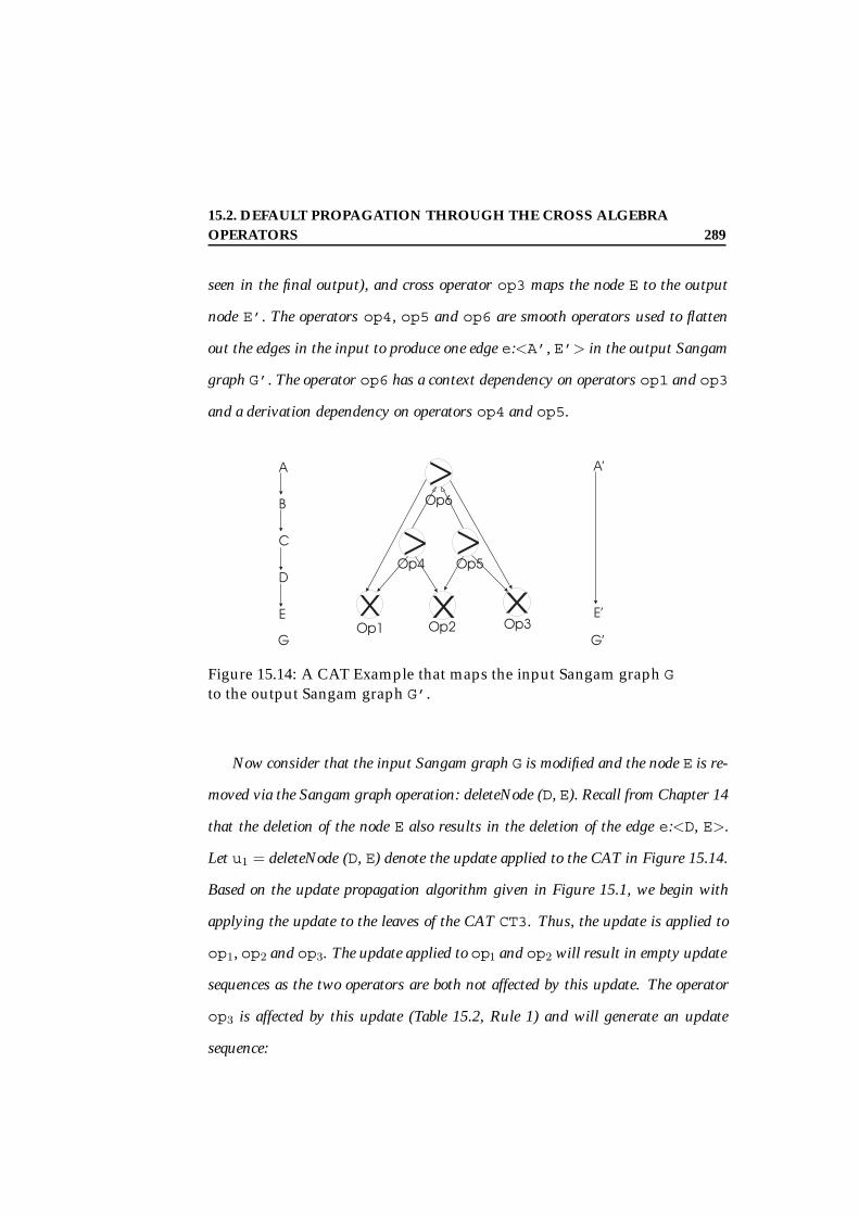
15.2. DEFAULT PROPAGATION THROUGH THE CROSS ALGEBRAOPERATORS 289
seen in the final output), and cross operator op3 maps the node E to the output
node E’. The operators op4, op5 and op6 are smooth operators used to flatten
out the edges in the input to produce one edge e:<A’, E’> in the output Sangam
graph G’. The operator op6 has a context dependency on operators op1 and op3
and a derivation dependency on operators op4 and op5.
Figure 15.14: A CAT Example that maps the input Sangam graph Gto the output Sangam graph G’.
Now consider that the input Sangam graph G is modified and the node E is re-
moved via the Sangam graph operation: deleteNode (D, E). Recall from Chapter 14
that the deletion of the node E also results in the deletion of the edge e:<D, E>.
Let u1 = deleteNode (D, E) denote the update applied to the CAT in Figure 15.14.
Based on the update propagation algorithm given in Figure 15.1, we begin with
applying the update to the leaves of the CAT CT3. Thus, the update is applied to
op1, op2 and op3. The update applied to op1 and op2 will result in empty update
sequences as the two operators are both not affected by this update. The operator
op3 is affected by this update (Table 15.2, Rule 1) and will generate an update
sequence:

15.2. DEFAULT PROPAGATION THROUGH THE CROSS ALGEBRAOPERATORS 290
δ =< u01 > (15.12)
where u1’ = deleteNode (D’, E’). Moreover, as E the input of this operator
has been deleted, the operator op3 is marked for deletion (Table 15.2, Rule 1).
The operator op3 has two parents op5 and op6. Based on the Gen Propagation
algorithm (Figure 15.1), the update sequence δ (Equation 15.12) produced by the
children operators is applied to the parent operator in order from left to right. Let
us first consider the operator op5. The update u1’ 2 δ is applied to op5. The
update u1 does not affect the operator op5. However, the original update u1 does
affect the operator op5 (Table 15.4, Rule 1) and generates an update u2’ = delete-
Edge (C’, l) where l is the label for edge e’:<C’, E’>. As the operator op3 is in
context relationship with the operator op5, the update sequence generated by the
operator op5 is a concatenation of the update produced by op3, u1’ and the update
produced by op5, i.e. u2’. Hence,
δ0 =< u01, u0
2 > (15.13)
where u2’ and u1’ are as given above. Moreover, as one of the inputs of the
operator op5, the edge e:<D, E> is deleted, the operator op5 is marked for deletion
(Table 15.4, Rule 1).
Similarly, the update sequence δ = < u1’ > produced by op3 is also applied to
the operator op6. Based on the update u1’ and u1, the condition given in Table 15.4
15.2. DEFAULT PROPAGATION THROUGH THE CROSS ALGEBRAOPERATORS 291
Rule 1 is false. Hence the operator op6 is not affected by the update u1’ or the
update u1. However, as the operator op6 has a context relationship with operator
op3, even though op6 is not affected by the updates in δ, the update sequence δ is
included in the final update sequence produced by operator op6. Thus,
δ00 = δop34. =< u1
0 > (15.14)
where δ” is the update sequence produced by op6.
Now consider again the operator op6 that derives from the operator op5, i.e.,
op6 is the parent operator of op5. The update sequence δ’ produced by op5 (Equa-
tion 15.13) is now applied to operator op6, one update at a time. We first apply the
update u1’ 2 δ’. Here u1’ = deleteNode (D’, E’). This update does not effect the
operator op6 (Table 15.4, Rule 1 - the condition is false). Next we apply the update
u2’ = deleteEdge (C’, l) where l is the label for the edge e’:<C’,E’>. As e’ is
one of the inputs of the operator op6 and the conditions in Table 15.4, Rule 2 are
true, we state that the operator op6 is affected by the update u2’. It produces an
update u3’ = deleteEdge (A’,l’) where l’ is the label of the edge e’’:<A’,E’>
(Table 15.4, Rule 2). Based on the Gen Propagation algorithm, as the operator
op6 derives from the operator op5, the update sequence δ’ produced by the opera-
tor op5 is discarded. Hence the update sequence produced as a result of applying
the update sequence δ’ (Equation 15.13) on the operator op6 is
4We use the subscript op3 to denote that this is the update sequence produced by op3

15.2. DEFAULT PROPAGATION THROUGH THE CROSS ALGEBRAOPERATORS 292
δop6 =< u30 > . (15.15)
The final update sequence δ” produced by op6 is the combination of δop3 (Equa-
tion 15.14) and δop6. Thus, the final update sequence δ” is:
δ00 =< u10, u3
0 > . (15.16)
Moreover, as one input of op6, e’:<C’, E’> is deleted, the operator op6 is
marked for deletion. As op6 is the root of the context tree CT3, the propagation
terminates at op6. The update sequence δ” is the final update sequence that must
be applied to the output Sangam graph G’.
In pass 2, we start at the root op6 of the CAT and do an in-order traversal of
the tree. As operator op6 is marked for deletion, this mark for deletion propagates
to all children operators from which op6 derives (Refer to Figure 15.5). By the
algorithm (Figure 15.5), the operators op4, op5 and op2 are marked for deletion.
The operators op1 and op3 are not marked for deletion as they are shared operators
(refer to Figure 15.5). At the end of the mark for deletion propagation, all operators
marked for deletion are removed from the CAG.
The updated output Sangam graph G’’ consists of two nodes A’ (output of
operator op1) and E’ (output of operator op3) that are disconnected. As the Sang-
am graph G’’ is not a well-formed Sangam graph (Definition 21), the update
process is aborted and the Sangam graph G’’ rolled back to the Sangam graph G’.

15.2. DEFAULT PROPAGATION THROUGH THE CROSS ALGEBRAOPERATORS 293
15.2.2 Propagation Rules for SAG-DU Operations
In Figures 15.6-15.9 we give the default propagation tables of the Sangam
graph data update (SAG-DU) operations for the four cross algebra opera-
tors. Recall from Chapter 12 that the notation o0(o) implies that the object
o’ is produced by a cross mapping of the object o. Each update case indi-
cates the behavior for the algebra operator when the conditions are true. If
the conditions are not true there is no effect on the algebra operator, i.e., no
updated sequence is generated by the operator.
SAG-DU Operation Condition Update ProducedaddObject (v, m) if m0(m) addObject (v, m’)
deleteObject (o, m)if m0(m) && o0(o) deleteObject (o’,m’)else no effect
addEdgeObject (o1,o2,e)
no effect no effect
deleteEdgeObject(oe:<o1, o2>, e)
no effect no effect
Table 15.6: Default SAG-DU Propagation Rules for m0(m).
Propagation By Example: A Sangam Graph Data Update Propagation Ex-
ample
Consider the CAT given in Figure 15.14. Now let the extent of the input
Sangam graph G of the CAT be modified by the Sangam graph primitive:
addObject (v, A). This operation creates a new object o with value v, and
then inserts o into the extent R (A). Let u1 = addObject (v, A) denote this
update to node A. To propagate this update u1 to the output Sangam graph
G’, we begin with the first pass of the Gen Propagation algorithm given in

15.2. DEFAULT PROPAGATION THROUGH THE CROSS ALGEBRAOPERATORS 294
SAG-DU Operation Condition Update ProducedaddObject (v, m) no effect
deleteObject (o, m)
if m0(m) && o0(o)&& e0 (e) && ifoe0 :<o1, o2> suchthat o’= o1 or o’=o2
deleteEdgeObject(oe0 ,e’))
else no effect
addEdgeObject (o1,o2,e)
if e0(e) && o0
1
(o1) && o0
2(o2)
addEdgeObject (o1’, o2’,e’)
else no effect
deleteEdgeObject (oe, e) if e0(e) &&oe0 (oe)
deleteEdgeObject (oe’,e’)
Table 15.7: Default SAG-DU Propagation Rules fore0 (e), where e’:<m’,n’> and e:<m, n>, and m0(m) and n0(n).
SAG-DU Operation Condition Update ProducedaddObject (v, m) no effect
deleteObject (o, m)
if m0(m) && o0(o)&&=e0 (e1, e2) &&oe0 :<o1, o2> suchthat o’= o1 or o’=o2
deleteEdgeObject(oe0 ,e’)
else no effectaddEdgeObject (o1,o2,e) no effect
deleteEdgeObject (oe, e)
if oe:<o1,o2 &&=e0(e1,e2) &&=oe0
(oe1’,oe2’) &&e = e1 or e = e2
deleteEdgeObject (oe’,e’)
Table 15.8: Default SAG-DU Propagation Rules for =e0 (e1, e2).
Figure 15.1. The update u1 is applied to each leaf operator op1, op2 and
op3 of the CAT shown in Figure 15.14. By the conditions given in Table 15.6
Rule 1, only operator op1 is affected by the update u1 producing an update
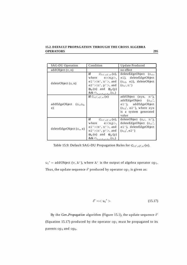
15.2. DEFAULT PROPAGATION THROUGH THE CROSS ALGEBRAOPERATORS 295
SAG-DU Operation Condition Update ProducedaddObject (v, m) no effect
deleteObject (o, m)
if <e10,e20,n0(e),where e:<m,p>,e1’:<m’, n’>, ande2’:<n’, p’>, andm0(m) and p0(p)&& <oe10 ,oe20 ,on0
(oe)
deleteEdgeObject (oe1,e1), deleteEdgeObject(oe2, e2), deleteObject(on0 , n’)
addEdgeObject (o1,o2,e)
if <e10,e20,n0(e) addObject (sys, n’),addEdgeObject (oe1’,e1’), addEdgeObject(oe2’, e2’), where sysis a system generatedvalue
deleteEdgeObject (oe, e)
if <e10,e20,n0(e),where e:<m,p>,e1’:<m’, n’>, ande2’:<n’, p’>, andm0(m) and p0(p)&& <oe10 ,oe20 ,on0
(oe)
deleteObject (on0 , n’),deleteEdgeObject (oe1’,e1’), deleteEdgeObject(oe2’, e2’)
Table 15.9: Default SAG-DU Propagation Rules for <e10,e20,n0(e).
u1’ = addObject (v, A’), where A’ is the output of algebra operator op1.
Thus, the update sequence δ’ produced by operator op1 is given as:
δ0 =< u10 > (15.17)
By the Gen Propagation algorithm (Figure 15.1), the update sequence δ’
(Equation 15.17) produced by the operator op1 must be propagated to its
parents op4 and op6.

15.2. DEFAULT PROPAGATION THROUGH THE CROSS ALGEBRAOPERATORS 296
Consider first the parent operator op65. The operator op6 is unaffected
by both the original update u1 (this must be applied as the two operators
are related by context dependency - refer Figure 15.1) and the update u1’
in the update sequence δ’ produced by operator op1. As the two operators
are associated by context dependency, the update sequence generated by
op6 is concatenated with the update sequence of op1. Thus, the update
sequence δ” produced by operator op6 is given as:
δ00 =< u10 > (15.18)
Next consider the operator op4. By the conditions given in Table 15.8
Rule 1, the operator op4 is not affected by the original update u1 and the
update u1’ and hence produces an empty update sequence. However, as
the operatorop4 is in context relationship with the operatorop1, the update
sequence δ’ produced by op1 must be concatenated with the final sequence
of the parent operator op4. Hence the update sequence δ”’ produced by
op4 is:
δ000 =< u10 > (15.19)
Propagating this update sequence to the parent operator op6 of op4, we
find that the operator op6 is unaffected by the update u1’ 2 δ”’ (by the5The actual order of propagation is irrelevant.

15.3. PROPERTIES OF PROPAGATION THROUGH CAGS 297
conditions of Table 15.8, Rule 1). Moreover, as operator op6 derives from
operator op4, the update sequence δ”” produced by op6 is empty. Hence,
δ0000 =<> (15.20)
The update propagation terminates with the operator op6 as op6 is the
root of the CAT CT3. The final update sequence produced by the opera-
tor op6 is the concatenation of the two update sequences produced by the
propagation of the update sequences of op1 (Equation 15.18) and operator
op4 (Equations 15.20). Hence, the final update sequence δfinal is given as:
δfinal =< u10 > (15.21)
As no operators are marked for deletion, the second pass (Figure 15.5)
will result only in the application of δfinal to the extent of the output Sang-
am graph G’, i.e., in the addition of a new object o’ with value v to the
extent I (A’) of node A’.
15.3 Properties of Propagation Through CAGs
15.3.1 Correctness of Propagation
An important property that must be satisfied by the propagation algo-
rithms, Gen Propagation and Insert Propagation , is the correctness of the re-

15.3. PROPERTIES OF PROPAGATION THROUGH CAGS 298
sultant output Sangam graph . That is, the algorithms must ensure that
the modified output Sangam graph Gu’ produced by applying the update
sequence is indeed a valid Sangam graph . For this we state the following
two results.
Lemma 11 (Propagation Correctness) The propagation of an update u through
a cross algebra graph CAG produces a well-formed cross algebra graph CAG’.
Let CAG represent the original CAG that maps the input Sangam graph
G to the output Sangam graph G’. Now let the input Sangam graph G be
modified by the application of an update operation u.
Case 1 (u = insertNode ): The insertNode (insertNodeAt ) operation is
propagated using the Insert Propagation algorithm. By the Insert Propagation
algorithm, the propagation of the insertNode operation produces a new
context dependency tree CT such that the modified CAG CAG’ is given as:
CAG0 = (CAG) Æ (CT) (15.22)
This is a well-formed CAG by definition (Definition 19).
Case 2 (u = insertEdge ): The same as above (for insertNode ) holds for
the propagation of the insertEdge (and insertEdgeAt ) operation using the
Insert Propagation algorithm.
Case 3 (u = deleteNode ): The deleteNode operation is propagated using
the Gen Propagation algorithm. For this operation, we consider the follow-
ing scenarios:

15.3. PROPERTIES OF PROPAGATION THROUGH CAGS 299
1. CAG = opi - Let CAG be a single operator opi. If the operator opi is
affected by the update deleteNode , it would imply that the input for
the operator opi has been deleted (Tables 15.2- 15.5). In this case the
operator opi is deleted. Thus, the updated cross algebra graph CAG’
= ; which is a valid cross algebra graph.
If the operator opi is not affected by the update deleteNode , then the
updated cross algebra graph CAG’ = CAG, and is hence well-formed
(Definition 19).
2. CAG = opi,opj - Let the CAG consist of two nodes that are connected
via a context dependency edge (represented by ‘,’ in the expression).
If the operators opi or opj are affected by the update deleteNode
, then they are deleted, resulting in one of the following scenarios:
CAG’ = opi, or CAG’ = opj , or CAG’ = ;.
If the two operators are not affected by the update deleteNode , then
CAG’ = opi,opj . In all of these cases, the cross algebra graph CAG’ is
a well-formed CAG (Definition 19).
3. CAG= opi(opj) - Let the cross algebra graph CAG consist of two oper-
ators opi and opj connected by a derivation edge. If the operator opj
is affected by the update deleteNode , then this will result in the dele-
tion of the operator opj and consequently the deletion of the operator
opi. In this case, CAG’ = ;.
If the operator opj is not affected by the update deleteNode then the
update is not propagated to operator opi, i.e., opi is also not affected

15.3. PROPERTIES OF PROPAGATION THROUGH CAGS 300
by the update. Hence, CAG’= opi(opj). In both of the cases, the final
CAG is a well-formed CAG (Definition 19).
4. CAG = opi Æ opj - This case can be treated in the same manner as (1).
Each of the above scenarios and the subsequent results can be extended
without loss of generality to larger CAGs.
Other Cases: The cases for deleteEdge , and rename also produce well-
formed CAGs. These can be argued similar to the discussions above.
The updates u = addObject , deleteObject , addEdgeObject , delete-
EdgeObject do not affect the structure of the CAG. Hence, if the cross
algebra graph CAG is well-formed, then CAG’ = CAG is also well-formed
after the application of an update u.
Lemma 12 (Valid Propagation) The propagation of an update u through a cross
algebra graph CAG produces a valid modified Sangam graph Gu’.
This result follows directly from Lemma 11.
15.3.2 Incremental Propagation Versus Recomputation
The Gen Propagation and the Insert Propagation algorithms are incremental
algorithms, i.e., an update applied on the input Sangam graph G is propa-
gated through the CAG and applied to the output Sangam graph G’ with-
out requiring the complete re-evaluation of the entire CAG. Both the in-
cremental propagation and the re-evaluation of the CAG will result in the
same modified output Sangam graph Gu’.
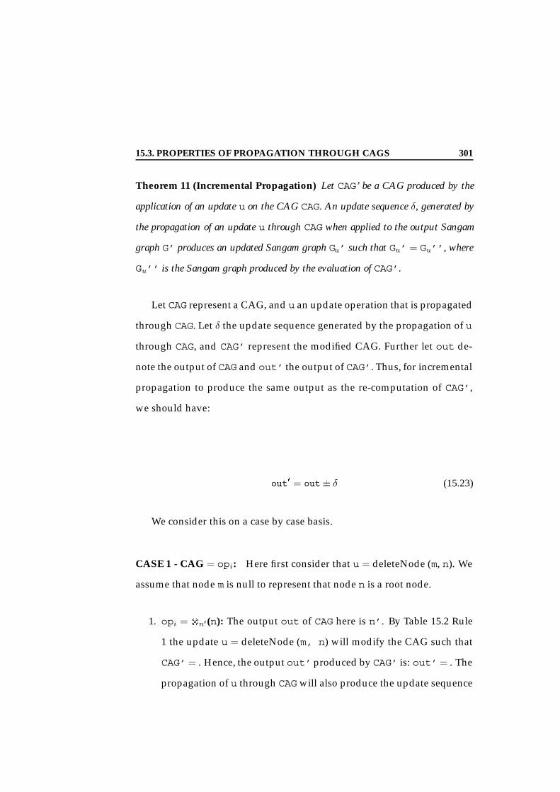
15.3. PROPERTIES OF PROPAGATION THROUGH CAGS 301
Theorem 11 (Incremental Propagation) Let CAG’ be a CAG produced by the
application of an update u on the CAG CAG. An update sequence δ, generated by
the propagation of an update u through CAG when applied to the output Sangam
graph G’ produces an updated Sangam graph Gu’ such that Gu’ = Gu’’, where
Gu’’ is the Sangam graph produced by the evaluation of CAG’.
Let CAG represent a CAG, and u an update operation that is propagated
through CAG. Let δ the update sequence generated by the propagation of u
through CAG, and CAG’ represent the modified CAG. Further let out de-
note the output of CAG and out’ the output of CAG’. Thus, for incremental
propagation to produce the same output as the re-computation of CAG’,
we should have:
out0 = out δ (15.23)
We consider this on a case by case basis.
CASE 1 - CAG = opi: Here first consider that u = deleteNode (m, n). We
assume that node m is null to represent that node n is a root node.
1. opi = n0(n): The output out of CAG here is n’. By Table 15.2 Rule
1 the update u = deleteNode (m, n) will modify the CAG such that
CAG’= . Hence, the output out’ produced by CAG’ is: out’= . The
propagation of u through CAG will also produce the update sequence
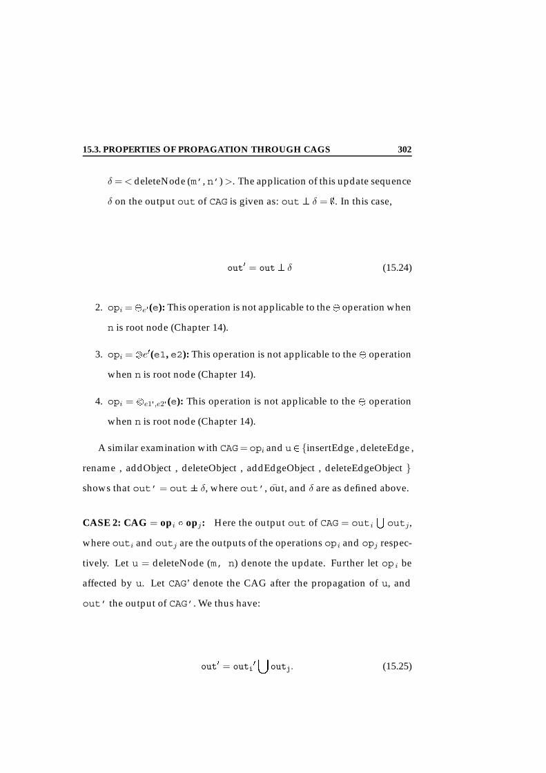
15.3. PROPERTIES OF PROPAGATION THROUGH CAGS 302
δ =< deleteNode (m’, n’)>. The application of this update sequence
δ on the output out of CAG is given as: out δ = ;. In this case,
out0 = out δ (15.24)
2. opi =e0(e): This operation is not applicable to the operation when
n is root node (Chapter 14).
3. opi ==e0(e1, e2): This operation is not applicable to the operation
when n is root node (Chapter 14).
4. opi = <e10,e20(e): This operation is not applicable to the operation
when n is root node (Chapter 14).
A similar examination with CAG= opi and u2 insertEdge , deleteEdge ,
rename , addObject , deleteObject , addEdgeObject , deleteEdgeObject shows that out’= out δ, where out’, out, and δ are as defined above.
CASE 2: CAG = opi Æ opj : Here the output out of CAG = outiSoutj,
where outi and outj are the outputs of the operations opi and opj respec-
tively. Let u = deleteNode (m, n) denote the update. Further let op i be
affected by u. Let CAG’ denote the CAG after the propagation of u, and
out’ the output of CAG’. We thus have:
out0 = outi0[
outj. (15.25)

15.3. PROPERTIES OF PROPAGATION THROUGH CAGS 303
The operation opj here is unaffected. By CASE 1, we know that if CAG
= opi, then out’ = out δ. Thus, we have outi’ = outi δ. Replacing
outi’ in Equation 15.25, we have:
out0 = (outi δ)[
outj. (15.26)
This result can be shown for the case when opj is affected or if both
opi and opj are affected. This result can also be extended without loss of
generality to CAGs.
CASE 3: CAG = opi, opj: Here the output out of CAG is given as out
= outiSoutj, where outi and outj are the outputs of the operations
opi and opj respectively. Recall that the symbol “,” here reflects a context
dependency relationship. Let u denote the update applied to CAG. Further
let opi be affected by u. Let CAG’ denote the modified CAG with output
out’. Thus, out’= outi’Soutj. Based on CASE 1 and similar to CASE
2, we can replace outi’ with outi δ, where δ = < u’ > and u’ is the
update produced by opi. Thus incremental propagation achieves the same
resultant output as recomputation. A similar argument can be made if only
operator opj is affected by the update u.
Now let us consider that both operators opi and opj are affected by
the update u such that δ = <u1’, u2’>, where ui’ and uj’ are the updates
generated by opi and opj respectively. Breaking down δ into individual
updates, and based on CASE 1 we have:

15.3. PROPERTIES OF PROPAGATION THROUGH CAGS 304
outi0 = outi ui
0 (15.27)
outj0 = outj uj
0 (15.28)
We know by definition (Definition 19), that out’ of the modified CAG
CAG’ when both opi and opj are affected is given as:
out0 = outi0[
outj0 (15.29)
Replacing outi’ and outj’ in Equation 15.29 using Equation 15.27 and
Equation 15.28, we have:
out0 = (outi ui0)[
(outj uj0) (15.30)
out0 = outi[
outj ui0 uj
0
out0 = outi[
outj δ
This result can be generalized to CAGs of arbitrary size.
CASE 4: CAG = opi(opj): Here the output out of CAG is given as out
= outi, where outi is the output of the outer most operation op i. Recall
that the symbol “( )” here reflects a derivation relationship. Also recall that

15.3. PROPERTIES OF PROPAGATION THROUGH CAGS 305
an outer operation is affected by an update only if its leaves are affected
by the update. Thus, let us assume that operation opj is affected by the
update u. Let δ = < u’ > be the updated generated by op j . We know by
the Gen Propagation propagation algorithm that only updates generated by
the children operators are applied to the parent operator. Hence, we apply
the update u’ on the operator opi. The original update u is not applied to
opi. Let δ’ = <u’’ denote the update generated by op i. By CASE 1, we
have:
outi0 = outi u00 (15.31)
This result can also be generalized to CAGs of arbitrary size.
The Insert Operations. We next consider the insertNode and insertEdge
operations. Let CAG = CAG1 Æ CAG2 . . . Æ CAGi be a CAG. Let the input SAG
G be modified by the update u 2 insertNode , insertNodeAt , insertEdge
, insertEdgeAt . We know by definition (Definition 19), the output of CAG
is given as: out = out1Sout2
S. . . outi. By the Insert Propagation algo-
rithm, the propagation of these operations always produces a new context
dependency tree CTj(out0j). The modified CAG is given as:
CAG0 = CAG1 Æ CAG2 . . . Æ CAGi Æ CTj (15.32)

15.4. SUMMARY 306
The output of CAG’ is given as:
out0 = out1[
out2 . . .[
outi[
out0j (15.33)
This can be re-written as:
out0 = out[
out0j (15.34)
where out is the output of CAG. Thus incremental propagation pro-
duces the same result as re-computation. 2
15.4 Summary
In this chapter, we have presented an incremental propagation algorithm
that can propagate the updates as presented in Chapter 14 through a cross
algebra expression, to produce a set of updates that can be applied on the
output Sangam graph. We have presented default propagation strategies
for each algebra operator and update; and have shown that incremental
propagation is equivalent to full recomputation. However, we should point
out that if the original cross algebra expression is built based on rules such
as the basic or shared inlining rules, then the default propagation rules for
the insert evolution operations cannot guarantee that the rules used for the

15.4. SUMMARY 307
construction of the cross algebra expression will be preserved after default
propagation.

15.4. SUMMARY 308
309
Chapter 16
Performance Comparison:
Incremental vs Re-computation
One of the key motivations for incremental propagation is the benefit to
performance, measured in terms of the total time taken to produce the up-
dated output, over re-computation. In this chapter, we present experimen-
tal results to: (1) show that incremental propagation has lower execution
times than re-computation; and (2) analyze the performance of the incre-
mental propagation for different cross algebra operators and different types
of cross algebra graphs.
All experiments used personal.dtd, represented in Figure 16.1 as the
input. The xmlPGen tool was used to generate the corresponding XML
documents with a uniform distribution of the number of objects that are
instances of the nodes and edges of the Sangam graph. The cross algebra
graphs (CAGs), ident and inline, and the different cross algebra operators
CHAPTER 16. PERFORMANCE COMPARISON: INCREMENTAL VSRE-COMPUTATION 310
were constructed as described in Section 13.2. All data update operations
involved the person, name and given elements. All data update opera-
tions were generated using a simple program that we wrote.
<?xml encoding="UTF-8"?><!ELEMENT personnel (person)+><!ELEMENT person (name,email*,url*,link?)><!ATTLIST person id ID #REQUIRED><!ATTLIST person note CDATA #IMPLIED><!ATTLIST person salary CDATA #IMPLIED>
<!ELEMENT name (family,given)>
<!ELEMENT family (#PCDATA)>
<!ELEMENT given (#PCDATA)>
<!ELEMENT email (#PCDATA)>
<!ELEMENT url EMPTY><!ATTLIST url href CDATA ’http://’>
<!ELEMENT link EMPTY><!ATTLIST link manager IDREF #IMPLIED><!ATTLIST link subordinates IDREFS #IMPLIED>
<!NOTATION gif PUBLIC ’-//APP/Photoshop/4.0’’photoshop.exe’>
Figure 16.1: The personal.dtd, used as the input DTD.
The re-computation time corresponds to the time taken to evaluate the
given cross algebra graph after a change to the input graph and does not
include the time required to build the cross algebra graph.
In all of the experiments below, we report the propagation times for var-
ious data update operations, i.e., insertObject, deleteObject, in-

CHAPTER 16. PERFORMANCE COMPARISON: INCREMENTAL VSRE-COMPUTATION 311
sertEdgeObjectand deleteEdgeObject. We do not consider any sch-
ema change operations. Typically, a schema change operation has (1) some
processing cost (pc), i.e., the cpu time taken to actually perform the change
once all data is in memory; and (2) some I/O cost (rw), i.e., the time re-
quired to read and write the data on which the change is applied to and
from the disk. The cost of the schema change operations is largely domi-
nated by this I/O cost. This I/O cost is dependent on the particular DBMS
system that was used and not on the middle-layer, i.e., the Sangam layer.
The processing cost, pc, is the only cost affected by the propagation algo-
rithm, the focus of this research. For schema changes this processing cost is
comparable to those reported for the data update operations but is scaled
according to the number of objects associated with the input node to which
the change is applied.
All experiments were conducted on a Pentium IV, 933MHz, 256MB RAM
system running Debian Linux, kernel version 2.2.19, using the Sangam pro-
totype system described in Section 7.1. The Sangam system itself was built
using the Java JDK version 1.3.1.
Pilot tests on our system showed that the time taken to incrementally
propagate the data change operations through a CAG were from 5 to 10
milliseconds. As typical operating systems clocks have a granularity of
about 10 milliseconds, we record the time taken to propagate 1000 change
operations. Average per operation measurements can be easily obtained
by dividing the reported results by 1000. In the graphs presented here we
report the time for 1000 change operations for both re-computation and
incremental propagations.
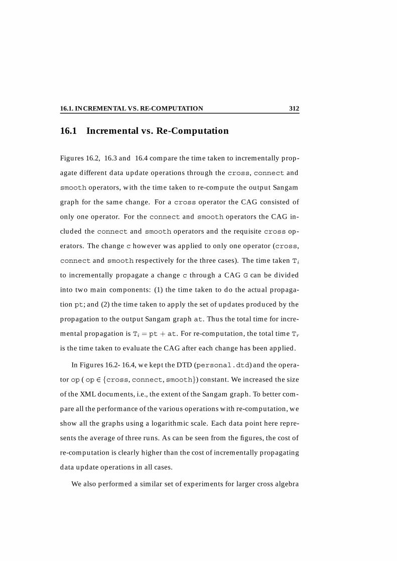
16.1. INCREMENTAL VS. RE-COMPUTATION 312
16.1 Incremental vs. Re-Computation
Figures 16.2, 16.3 and 16.4 compare the time taken to incrementally prop-
agate different data update operations through the cross, connect and
smooth operators, with the time taken to re-compute the output Sangam
graph for the same change. For a cross operator the CAG consisted of
only one operator. For the connect and smooth operators the CAG in-
cluded the connect and smooth operators and the requisite cross op-
erators. The change c however was applied to only one operator (cross,
connect and smooth respectively for the three cases). The time taken Ti
to incrementally propagate a change c through a CAG G can be divided
into two main components: (1) the time taken to do the actual propaga-
tion pt; and (2) the time taken to apply the set of updates produced by the
propagation to the output Sangam graph at. Thus the total time for incre-
mental propagation is Ti = pt + at. For re-computation, the total time Tr
is the time taken to evaluate the CAG after each change has been applied.
In Figures 16.2- 16.4, we kept the DTD (personal.dtd) and the opera-
tor op ( op 2 cross, connect, smooth) constant. We increased the size
of the XML documents, i.e., the extent of the Sangam graph. To better com-
pare all the performance of the various operations with re-computation, we
show all the graphs using a logarithmic scale. Each data point here repre-
sents the average of three runs. As can be seen from the figures, the cost of
re-computation is clearly higher than the cost of incrementally propagating
data update operations in all cases.
We also performed a similar set of experiments for larger cross algebra
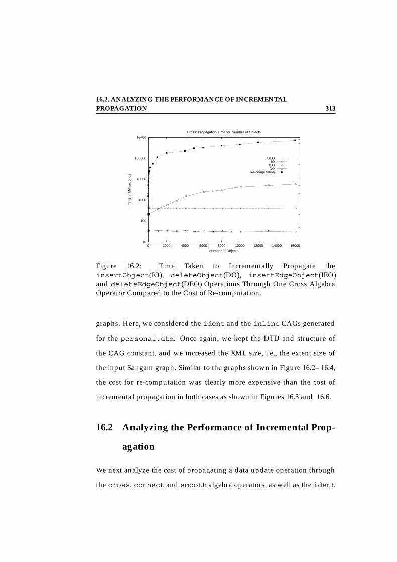
16.2. ANALYZING THE PERFORMANCE OF INCREMENTALPROPAGATION 313
10
100
1000
10000
100000
1e+06
0 2000 4000 6000 8000 10000 12000 14000 16000
Tim
e in
Mill
isec
onds
Number of Objects
Cross: Propagation Time vs. Number of Objects
DEOIO
IEODO
Re-computation
Figure 16.2: Time Taken to Incrementally Propagate theinsertObject(IO), deleteObject(DO), insertEdgeObject(IEO)and deleteEdgeObject(DEO) Operations Through One Cross AlgebraOperator Compared to the Cost of Re-computation.
graphs. Here, we considered the ident and the inline CAGs generated
for the personal.dtd. Once again, we kept the DTD and structure of
the CAG constant, and we increased the XML size, i.e., the extent size of
the input Sangam graph. Similar to the graphs shown in Figure 16.2– 16.4,
the cost for re-computation was clearly more expensive than the cost of
incremental propagation in both cases as shown in Figures 16.5 and 16.6.
16.2 Analyzing the Performance of Incremental Prop-
agation
We next analyze the cost of propagating a data update operation through
the cross, connect and smooth algebra operators, as well as the ident

16.2. ANALYZING THE PERFORMANCE OF INCREMENTALPROPAGATION 314
100
1000
10000
100000
1e+06
1e+07
1e+08
0 2000 4000 6000 8000 10000 12000 14000 16000
Tim
e in
Mill
isec
onds
Number of Objects
Connect: Propagation Time vs. Number of Objects
DEOIO
IEODO
Re-computation
Figure 16.3: Time Taken to Incrementally Propagate the insertObject(IO), deleteObject(DO), insertEdgeObject(IEO) anddeleteEdgeObject(DEO) Operations Through One Connect Alge-bra Operator Compared to the Cost of Re-computation.
and the inline CAGs.
16.2.1 The Algebra Operators
Cross Algebra Operator
Figure 16.7 depicts the time taken to propagate the different data update
operations, insertObject, deleteObject, insertEdgeObject and
deleteEdgeObject, through a cross algebra operator. Here we kept the
input DTD and the cross algebra operator constant, and increased the num-
ber of input objects. Each data point represents the average of three runs.
The insertObject inserts an object into the Sangam graph. The cost
to perform this operation is constant and does not vary with the input ex-

16.2. ANALYZING THE PERFORMANCE OF INCREMENTALPROPAGATION 315
100
1000
10000
100000
1e+06
1e+07
1e+08
1e+09
0 2000 4000 6000 8000 10000 12000 14000 16000
Tim
e in
Mill
isec
onds
Number of Objects
Smooth: Propagation Time vs. Number of Objects
DEOIO
IEODO
Re-computation
Figure 16.4: Time Taken to Incrementally Propagate theinsertObject(IO), deleteObject(DO), insertEdgeObject(IEO)and deleteEdgeObject(DEO) operations Through One Smooth AlgebraOperator Compared to the Cost of Re-computation.
tent size. Hence, the application time at is constant. Moreover, as the
cross algebra operator is kept constant, the propagation time pt is also
constant. This is depicted by the horizontal line depicting the propagation
of the insertObject in Figure 16.7.
The deleteObjectoperation deletes the object with the specified value
from the extent of the specified node. To apply this operation, we must
first find the correct object in the extent prior to constructing the update
to be applied on the output. The cost of searching for the correct object,
and hence the propagation time, pt, increases linearly with a linear in-
crease in the extent size. The application cost at is constant. As depicted
in Figure 16.7, the total time for propagating the deleteObject operation
16.2. ANALYZING THE PERFORMANCE OF INCREMENTALPROPAGATION 316
1000
10000
100000
1e+06
1e+07
1e+08
1e+09
0 2000 4000 6000 8000 10000 12000 14000 16000
Tim
e in
Mill
isec
onds
Number of Objects
Ident: Propagation Time vs. Number of Objects
DEOIO
IEODO
Re-computation
Figure 16.5: Time Taken to Incrementally Propagate theinsertObject(IO), deleteObject(DO), insertEdgeObject(IEO)and deleteEdgeObject(DEO) Operations Through an Ident CAGCompared to the Cost of Re-computation.
through a cross algebra operator thus increases linearly with the number of
objects in the extent.
As can be seen in Figure 16.7, the insertEdgeObject and delete-
EdgeObjecthave a negligible cost since these operators are not applicable
to cross operator (Section 15.2).
Connect Algebra Operator
Figure 16.8 depicts the time taken to propagate the different data update
operations, insertObject, deleteObject, insertEdgeObject and
deleteEdgeObject, through a connect algebra operator. Here, we also
kept the input DTD and the connect algebra operator constant, and in-

16.2. ANALYZING THE PERFORMANCE OF INCREMENTALPROPAGATION 317
1000
10000
100000
1e+06
1e+07
1e+08
1e+09
1e+10
0 2000 4000 6000 8000 10000 12000 14000 16000
Tim
e in
Mill
isec
onds
Number of Objects
Inline: Propagation Time vs. Number of Objects
DEOIO
IEODO
Re-computation
Figure 16.6: Time Taken to Incrementally Propagate theinsertObject(IO), deleteObject(DO), insertEdgeObject(IEO)and deleteEdgeObject(DEO) Operations Through an Inline CAGCompared to the Cost of Re-computation.
creased the number of input objects. Each data point represents the average
of three runs.
The insertObject operation is not applicable to the connect alge-
bra operator (refer Table 15.7). Hence, the application time at = 0. The
propagation time pt, and hence the total time T, is constant as depicted in
Figure 16.8.
The propagation time pt for thedeleteObject,deleteEdgeObject
and insertEdgeObjectoperations increases linearly with the increase in
the extent size. Once the set of updates are produced the amount of time
taken to apply one update at is constant. Hence, the total time T = pt
+ C, where C is some constant value for applying the change for all the

16.2. ANALYZING THE PERFORMANCE OF INCREMENTALPROPAGATION 318
0
1000
2000
3000
4000
5000
6000
7000
0 2000 4000 6000 8000 10000 12000 14000 16000
Tim
e in
Mill
isec
onds
Number of Objects
Cross: Propagation Time vs. Number of Objects
DEOIO
IEODO
y = .37 + 134
Figure 16.7: Time Taken to Incrementally Propagate theinsertObject(IO), deleteObject(DO), insertEdgeObject(IEO)and deleteEdgeObject(DEO) Operations Through the cross AlgebraOperator.
operations, increases linearly with the increase in the extent size of the in-
put. The variation in the slope of the lines is largely due to the cost of the
searches that must be performed to find the affected objects in the output
Sangam graph and construct the correct update operation during the prop-
agation. For example, for a deleteObject operation we must find all the
edges that have the specified object o on either end of the edge (see Ta-
ble 15.7), and then construct the correct deleteEdgeObject operations.
In contrast, while the insertEdgeObject has considerable propagation
cost, it will produce only one update in the case of the connect operator,
accounting for the slower increase in the update propagation times.

16.2. ANALYZING THE PERFORMANCE OF INCREMENTALPROPAGATION 319
0
5000
10000
15000
20000
25000
0 2000 4000 6000 8000 10000 12000 14000 16000
Tim
e in
Mill
isec
onds
Number of Objects
Connect: Propagation Time vs. Number of Objects
DEOIO
IEODO
Figure 16.8: Time Taken to Incrementally Propagate theinsertObject(IO), deleteObject(DO), insertEdgeObject(IEO)and deleteEdgeObject(DEO) Operations Through one connectAlgebra Operator.
Smooth Algebra Operator
Figure 16.9 depicts the time taken to propagate the different data update
operations, insertObject, deleteObject, insertEdgeObject and
deleteEdgeObject, through a smooth algebra operator. Here, we once
again keep the input DTD and the smooth algebra operator constant, and
increase the number of input objects. Each data point represents the aver-
age of three runs.
As in the case of the connect operator, the insertObject is not ap-
plicable to the smooth algebra operator (see Table 15.8). Hence, the appli-
cation time at = 0. The propagation time pt, and thus the total time T, is
constant as depicted by the horizontal line in Figure 16.9.

16.2. ANALYZING THE PERFORMANCE OF INCREMENTALPROPAGATION 320
0
5000
10000
15000
20000
25000
30000
35000
40000
45000
50000
0 2000 4000 6000 8000 10000 12000 14000 16000
Tim
e in
Mill
isec
onds
Number of Objects
Smooth: Propagation Time vs. Number of Objects
DEOIO
IEODO
Figure 16.9: Time Taken to Incrementally Propagate theinsertObject(IO), deleteObject(DO), insertEdgeObject(IEO)and deleteEdgeObject(DEO) Operations Through One Smooth Alge-bra Operator.
The propagation times pt for the deleteObject,deleteEdgeObject
and insertEdgeObjectoperations increases linearly with the increase in
the extent size. The variation in the slope of the total times for the delete-
Object, deleteEdgeObject and the insertEdgeObject are as before
due to the increasing search space to locate the correct objects in the output
Sangam graph and construct the required updates.
Comparison of Propagation Times for Different Operators
In summary, the propagation of the data update operations through the dif-
ferent algebra operators depict similar trends. As expected for the cross
operator, the cost of incrementally propagating the insertEdgeObject
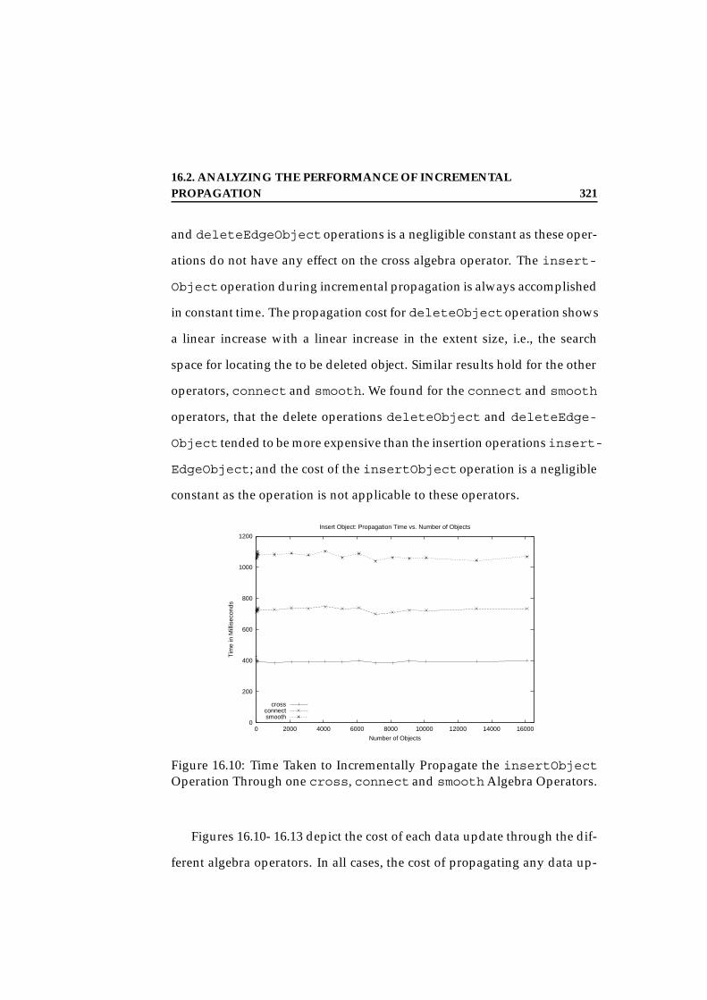
16.2. ANALYZING THE PERFORMANCE OF INCREMENTALPROPAGATION 321
and deleteEdgeObjectoperations is a negligible constant as these oper-
ations do not have any effect on the cross algebra operator. The insert-
Object operation during incremental propagation is always accomplished
in constant time. The propagation cost for deleteObjectoperation shows
a linear increase with a linear increase in the extent size, i.e., the search
space for locating the to be deleted object. Similar results hold for the other
operators, connect and smooth. We found for the connect and smooth
operators, that the delete operations deleteObject and deleteEdge-
Object tended to be more expensive than the insertion operationsinsert-
EdgeObject; and the cost of the insertObject operation is a negligible
constant as the operation is not applicable to these operators.
0
200
400
600
800
1000
1200
0 2000 4000 6000 8000 10000 12000 14000 16000
Tim
e in
Mill
isec
onds
Number of Objects
Insert Object: Propagation Time vs. Number of Objects
crossconnectsmooth
Figure 16.10: Time Taken to Incrementally Propagate the insertObjectOperation Through one cross, connect and smooth Algebra Operators.
Figures 16.10- 16.13 depict the cost of each data update through the dif-
ferent algebra operators. In all cases, the cost of propagating any data up-

16.2. ANALYZING THE PERFORMANCE OF INCREMENTALPROPAGATION 322
0
5000
10000
15000
20000
25000
30000
35000
40000
45000
50000
0 2000 4000 6000 8000 10000 12000 14000 16000
Tim
e in
Mill
isec
onds
Number of Objects
Delete Object: Propagation Time vs. Number of Objects
crossconnectsmooth
Figure 16.11: Time Taken to Incrementally Propagate the deleteObjectOperation Through one cross, connect and smooth Algebra Operators.
date through the smooth operator is higher than the cost of propagating
the same update through the connect and cross operators. This is pri-
marily because each operation requires more number of the searches when
applied to the smooth operator, thereby explaining the elevated costs.
0
5000
10000
15000
20000
0 2000 4000 6000 8000 10000 12000 14000 16000
Tim
e in
Mill
isec
onds
Number of Objects
Insert Edge Object: Propagation Time vs. Number of Objects
crossconnectsmooth
Figure 16.12: Time Taken toIncrementally Propagate theinsertEdgeObject OperationThrough one cross, connectand smooth Algebra Operators.
0
5000
10000
15000
20000
25000
30000
35000
40000
45000
0 2000 4000 6000 8000 10000 12000 14000 16000
Tim
e in
Mill
isec
onds
Number of Objects
Delete Edge Object: Propagation Time vs. Number of Objects
crossconnectsmooth
Figure 16.13: Time Taken toIncrementally Propagate thedeleteEdgeObject OperationThrough one cross, connectand smooth Algebra Operators.
16.2. ANALYZING THE PERFORMANCE OF INCREMENTALPROPAGATION 323
16.2.2 Ident and Inline CAGs
Variation in Extent Size
Figures 16.14 and 16.15 depict the cost of propagating the different data
updates through an ident and an inline CAG. For each experiment,
we kept the input DTD and the CAG structure constant, and linearly in-
creased the size of the input XML documents, i.e., the number of objects
in the input extent. Each data point represents the average of three runs.
Overall, we find that the performance of the insertObject operation in
both cases is a constant. The propagation costs for the other three oper-
ations, deleteObject, deleteEdgeObject and insertEdgeObject,
increases linearly with the linear increase in the extent size. The perfor-
mance costs for the deleteObject and the deleteEdgeObject were
once again higher than those for the insertEdgeObject operation due
to the increased search spaces for constructing the updates.
Figures 16.16- 16.18 compare the cost of propagating the different up-
date operations for the ident and inline CAGs. In all cases, the cost of
propagating the data updates through the inline CAG are higher than
the cost of propagating the same change through the ident CAG. The
ident CAG consists of cross and connect operators, that form many
separate, smaller CATs with a large number of shared operators. On the
other hand, the inline CAG contains fewer number of algebra operators,
but these operators are some composition of cross, connect and smooth
operators. The number of shared operators, in general, is fewer than in
the inline CAG. The performance of the propagation algorithm is not af-

16.2. ANALYZING THE PERFORMANCE OF INCREMENTALPROPAGATION 324
0
10000
20000
30000
40000
50000
60000
0 2000 4000 6000 8000 10000 12000 14000 16000
Tim
e in
Mill
isec
onds
Number of Objects
Ident: Propagation Time vs. Number of Objects
DEOIO
IEODO
Figure 16.14: Time Taken to Incrementally Propagate the insertObject,deleteObject, insertEdgeObject and deleteEdgeObject Opera-tions Through the ident CAG.
fected by the number of shared operators, as each must still be examined
in the context of new parents to determine the overall effect of the update.
We thus attribute the difference in the performance of the update propaga-
tion to the fact that the inlineCAG contains smooth operators which are
expensive for propagation.
Variation in Structure Size
To examine the effects of the CAG size on the performance of the update
propagation algorithm, we also conducted some experiments that varied
the size of the DTD, i.e., the number of elements in the DTD, causing a rel-
ative increase in the size of the resultant CAG. For this set of experiments,
we kept the extent size of the XML documents (and hence the extent size

16.2. ANALYZING THE PERFORMANCE OF INCREMENTALPROPAGATION 325
0
10000
20000
30000
40000
50000
60000
70000
80000
90000
100000
0 2000 4000 6000 8000 10000 12000 14000 16000
Tim
e in
Mill
isec
onds
Number of Objects
Inline: Propagation Time vs. Number of Objects
DEOIO
IEODO
Figure 16.15: Time Taken to Incrementally Propagate the insertObject,deleteObject, insertEdgeObject and deleteEdgeObject Opera-tions Through the inline CAG.
0
500
1000
1500
2000
2500
3000
3500
4000
4500
0 2000 4000 6000 8000 10000 12000 14000 16000
Tim
e in
Mill
isec
onds
Number of Objects
Insert Object: Propagation Time vs. Number of Objects
identinline
Figure 16.16: Time Taken to Incrementally Propagate the insertObject(IO) Operation Through the ident and inline CAG.

16.2. ANALYZING THE PERFORMANCE OF INCREMENTALPROPAGATION 326
0
5000
10000
15000
20000
25000
30000
35000
40000
0 2000 4000 6000 8000 10000 12000 14000 16000
Tim
e in
Mill
isec
onds
Number of Objects
Delete Object: Propagation Time vs. Number of Objects
identinline
Figure 16.17: Time Taken to Incrementally Propagate thedeleteObject(DO) Operation Through the ident and inline CAG.
0
5000
10000
15000
20000
25000
30000
35000
40000
0 2000 4000 6000 8000 10000 12000 14000 16000
Tim
e in
Mill
isec
onds
Number of Objects
Insert Edge Object: Propagation Time vs. Number of Objects
identinline
Figure 16.18: Time Taken to Incrementally Propagate theinsertEdgeObject(IEO) Operation Through the ident and inlineCAG.

16.2. ANALYZING THE PERFORMANCE OF INCREMENTALPROPAGATION 327
0
10000
20000
30000
40000
50000
60000
70000
80000
90000
100000
0 2000 4000 6000 8000 10000 12000 14000 16000
Tim
e in
Mill
isec
onds
Number of Objects
Delete Edge Object: Propagation Time vs. Number of Objects
identinline
Figure 16.19: Time Taken to Incrementally Propagate thedeleteEdgeObject(DEO) Operation Through the ident and inlineCAG.
of the Sangam graph ) constant at a uniform distribution of 10000 objects,
and varied the DTD and consequently the structure of the CAG. Each data
point represents the average of three runs.
Figures 16.20- 16.23 show the results of our experiments. In general,
we found that the performance of the update propagation algorithm for
each data update increased with a linear increase in the number of oper-
ators in the CAG. This result holds for both ident and inline CAGs.
The increase in the propagation costs for the insertObjectand delete-
Object operations was very small; and the propagation costs for the in-
sertEdgeObject and deleteEdgeObject operations showed a loga-
rithmic increase with a linear increase in the CAG size. While the trends for
the propagation of each operation were similar for both ident and inline
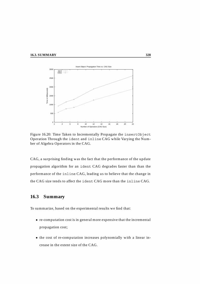
16.3. SUMMARY 328
0
500
1000
1500
2000
2500
3000
2 4 6 8 10 12 14 16 18 20 22
Tim
e in
Mill
isec
onds
Number of Operators (CAG Size)
Insert Object: Propagation Time vs. CAG Size
identinline
Figure 16.20: Time Taken to Incrementally Propagate the insertObjectOperation Through the ident and inline CAG while Varying the Num-ber of Algebra Operators in the CAG.
CAG, a surprising finding was the fact that the performance of the update
propagation algorithm for an ident CAG degrades faster than than the
performance of the inline CAG, leading us to believe that the change in
the CAG size tends to affect the ident CAG more than the inline CAG.
16.3 Summary
To summarize, based on the experimental results we find that:
• re-computation cost is in general more expensive that the incremental
propagation cost;
• the cost of re-computation increases polynomially with a linear in-
crease in the extent size of the CAG.

16.3. SUMMARY 329
0
2000
4000
6000
8000
10000
5 10 15 20
Tim
e in
Mill
isec
onds
Number of Operators(CAG Size)
Delete Object: Propagation Time vs. CAG Size
identinline
Figure 16.21: Time Taken to Incrementally Propagate the deleteObjectOperation Through the ident and inline CAG while Varying the Num-ber of Algebra Operators in the CAG.
0
5000
10000
15000
20000
25000
30000
2 4 6 8 10 12 14 16 18 20 22
Tim
e in
Mill
isec
onds
Number of Operators (CAG Size)
Insert Edge Object: Propagation Time vs. CAG Size
identinline
Figure 16.22: Time Taken to Incrementally Propagate theinsertEdgeObject Operation Through the ident and inlineCAG while Varying the Number of Algebra Operators in the CAG.

16.3. SUMMARY 330
0
5000
10000
15000
20000
25000
30000
35000
40000
45000
50000
2 4 6 8 10 12 14 16 18 20 22
Tim
e in
Mill
isec
onds
Number of Operators (CAG Size)
Delete Edge Object: Propagation Time vs. CAG Size
identinline
Figure 16.23: Time Taken to Incrementally Propagate thedeleteEdgeObject Operation Through the ident and inlineCAG while Varying the Number of Algebra Operators in the CAG.
• the cost of propagation for the operation insertObject is constant
for all algebra operators;
• the cost of propagation for the all updates increases linearly with lin-
ear increase in extent size for all CAGs;
• the cost of propagation for updates deleteEdgeObject and in-
sertEdgeObject increases logarithmically with a linear increase in
CAG size; while the cost of propagation for updates deleteObject
and insertObject show a negligible increase in performance cost
with a linear increase in CAG size.

331
Chapter 17
Related Work
17.1 XML Storage
Currently there are numerous projects that deal with the persistent storage
of XML documents [ZLMR01, FK99, SHT+99, CFLM00]. Shanmugasun-
daram et al. [SHT+99] presented the first storage of XML documents with
DTD in a relational system and cataloged the problems and limitations of
relational systems in doing so. In the same vein, Florescu et al. [FK99]
in their work present eight mapping schemes for storing XML documents
in relational databases with experimental data presented to help select an
ideal mapping scheme. Zhang et al. [ZLMR01] present one fixed mapping
for storing XML documents (with DTD) in relational systems. Catania et
al. [CFLM00] present the use of object databases to efficiently store XML
documents with DTDs. With the exception of the Clock project [ZLMR01],
none of these projects look at the maintenance of the relational or the object
storage when the source XML/DTD is modified. Zhang et al. [ZLMR01]

17.2. CHANGE MANAGEMENT 332
address this problem but only for their one fixed mapping. In our work, we
now provide an algebra that allows us to not only map XML documents to
relational, extended relational or object databases, but to also propagate
any DTD change to the same independent of the mapping.
17.2 Change Management
17.2.1 Change Propagation within A Data Model
In the relational database framework, much work has been done on the up-
date propagation from the view relations to the base relations [BS81, DB78,
Kel82] and maintenance of views [ZGMHW95, GB95]. Most of these al-
gorithms recompute the relational select-project-join views. Keller [Kel82]
proposed a methodology for translating updates against a view to updates
against the database. He proposed five criteria which must be satisfied by
all join translations. His work probably comes the closest to our work in
terms of translation of change from a view to the base. However, while
he looked at data updates in the relational model, we focus on the transla-
tion of schema updates in the object-oriented context. In view maintenance
work, Gupta et al. [GB95] proposed an algorithm for the maintenance of a
view defined using a deductive query language.
Object-oriented views are largely categorized as object preserving views
or object generating views. Bertino et al. [BCGMG97] have proposed a for-
mal framework for the definition of views. However, while they briefly
mention that update propagation is being investigated, this work is really
not reported in the paper. From the literature survey most work on up-

17.2. CHANGE MANAGEMENT 333
date of views in the OO context has been done on object-preserving views
[SLT91, San95, KR98]. In [GGMS97], Gluche et al. have proposed the incre-
mental maintenance of object views. Their work uses algebraic properties
of the materialized functions to decide if incremental update propagation
is feasible. They regard update operations as monoids and any update that
can be translated into a monoid is applicable for propagation. In [AYBS97],
Amer-Yahia et al. present an update propagation mechanism for views de-
fined in O2. This mechanism extends the view definition language to allow
the user to specify both the propagation as well as code that can be exe-
cuted when adding, deleting or modifying instances at the base class. For
example, the creation of a new object in a class Adult, a view defined over
a general class Person can be represented as follows in O2:
on create in class Adult with (name:String,
home:Address)
do Persons += set(self->root-object);
enddo;
Here, the class Person is identified as the base object to which the
change is propagated. In this example, the default rules for creation at the
base are utilized. However, OQL statements can be supplied as part of the
do clause to handle specific code.
In the context of schema changes through views, [RR97] have used
views as a mechanism to hide schema changes in the underlying database
from the applications that are defined on it. In doing so, this mechanism al-
lows the user to submit schema changes against a view which then need to

17.2. CHANGE MANAGEMENT 334
be propagated down to the base class as well as from the base to the view.
Other than this work, Breche et al. [BFK95] have proposed using views for
simulating schema changes. They look at simulating high-level primitives
(complex changes) [Bre96] using an enhanced O2 view mechanism. A user
can specify all changes and these are translated into schema propagation
changes when the user is ready to materialize their changes. The views
used for simulation are materialized views. Thus the base data is migrated
towards the data in the simulated view. This migration is when beyond the
default functionality is completely specified by the user via designer conver-
sion functions.
17.2.2 Supporting Applications During Change
Another important issue focuses on providing support for existing appli-
cations that depend on the old schema, when other applications change
the shared schema according to their own requirements. Research to ad-
dress this issue has followed along two possible directions, namely, views
[RLR98, RR97, Ber92] and versions [SZ86, Lau97b]. These approaches rely
on redundant information to continually support views and are examined
mainly in the context of data-warehousing.
Query Language Extensions
In the project, Evolvable View Environment (EVE), Rundensteiner et al. uti-
lize the redundancy in the information space to provide alternate sources
for the same information. They propose an extension to SQL, called E-SQL
17.2. CHANGE MANAGEMENT 335
[RLN97a] which allows the user to express tolerance levels for the alternate
information at the time of defining the query. This is particularly useful in a
distributed or a federated environment where information about one class,
say the Student class, is stored in more than one database and the user
is aware of this replication. Thus, if we were to consider the given schema
as being one in a large federation of schemas, then we could utilize the al-
ternate sources for re-writing the queries. For example, if the user specifies
that the class Student is equivalent to or some sub-set of it is equivalent
to the class Student’ in a different schema, then when the class Student
is deleted by the schema evolution operation delete-class, we can do a
query re-write using Student’. EVE offers many query language exten-
sions for the distributed environment.
Another approach that uses query language extensions is AQL [Har94].
AQL provides extension to OQL to handle traversals by specifying a start-
ing point and an ending point. However, this can handle only a limited
set of schema evolution changes, particularly schema changes that alter
the traversal paths. It cannot handle changes to traversal paths that are of
length one. Similar proposal for path traversal has also been made by Kifer
et al. [KKS92] in the language XSQL.
Hiding the Schema Change
Another approach that is perhaps more applicable in an environment where
a replacement of information is not possible is the one proposed by Run-
densteiner et al. in TSE - Transparent Schema Evolution [RR97]. TSE gives
its users the impression that the requested schema evolution operation has

17.2. CHANGE MANAGEMENT 336
been performed, while in reality it only simulates it for the application or
user that requested the change. This simulation of schema changes is done
via a view mechanism which hides the change from the user. Other queries
are unaffected as in their perception a change has not occurred. Using this
approach queries do not need to be re-written. Similarly, a add change is
propagated and applied to the base. Other queries defined on the same
base are re-written to effectively project now less information than is avail-
able at the base.
A similar approach is taken by versioning [MS93, KC88, Lau96, Lau97a].
When a schema change is submitted, a new version of the schema is cre-
ated. Older applications and queries can utilize the older schema version.
Once again as in views, no re-write of the application or queries is required.
However, versioning has its own set of problems that need to be resolved.
Objects that are now created in the newer version need to be propagated
backwards while objects created in the older version need to be propagated
forward. Similar to views there can be a proliferation of versions and the
system has to decide when it is possible to purge some versions.
17.2.3 XML Update Systems
The issue of change as well as that of propagating change from the source to
the target has been looked at in other contexts. Schema evolution systems
[Obj93, Cor00, SKC+01, CJR98c] exist both commercially as well as in re-
search projects and deal with structural changes in object database [Obj93]
and relational databases [Cor00]. However, they do not deal with the prop-
agation of change to targets that are derived from the now updated source.

17.3. SCHEMA INTEGRATION AND DATA TRANSFORMATION 337
In our previous work, we have developed XEM (XML Evolution Man-
ager) [SKC+01], a taxonomy of schema evolution operations for a DTD and
the corresponding set of XML documents. As part of this system we have
also shown how the XML changes can be propagated to an object reposi-
tory. Within XML there has been recent work done on propagation of XML
updates to the underlying relational database system by Tatarinov et al.
[TIHW01]. In their work, they describe a set of update methods for XML
documents, present how existing XML query languages can be extended to
support these update methods and finally show how these updates can be
propagated to the persistent relational database system.
17.2.4 Other Related Work.
Rosenthal et al. [RS99a] have proposed a propagation framework that
they have applied in the context of meta-data propagation in large multi-
tier databases and also in the context of security information propagation
through different levels of views. Our work is similar in that we apply the
notion of propagation from the view to the base. However, most of our
work is done with regards to the evolution of views.
17.3 Schema Integration and Data Transformation
There has been and continues to be much activity in the area of schema
transformation and integration [HMN+99, MZ98, FK99, MIR93, CJR98c,
RR87]. However, this work is typically specific to either the application do-
main or to a particular data model and does not deal with meta-modeling

17.3. SCHEMA INTEGRATION AND DATA TRANSFORMATION 338
[MR83, AT96, BR00, PR95, RR87]. Recent work related to ours are Clio
[HMN+99] a research project at IBM’s Almaden Research Center and work
by Milo and Zohar [MZ98]. Clio, a tool for creating mappings between two
data representations semi-automatically (i.e., with user input) focuses on
supporting querying of data in either the source or the target representation
and on just in time cleansing and transformation of data. Milo et al. [MZ98]
have looked at the problem of data translations based on schema-matching.
They follow an approach similar to Atzeni et al.[AT96] and Papazoglou et
al. [PR95] in that they define a set of translation rules to enable discovery
of relationships between two application schemas. We can directly make
use of translation algorithms from the literature, such as the algorithms for
translating between an XML-DTD and relational schema [FK99] or map-
ping rules [MZ98], and represent them as cross algebra graphs. However,
our focus is not discovering such algorithms for mapping but rather on
the generic expressibility of any possible (future) mapping and its manage-
ment. Work on equivalence of the translations between models [MIR93] is
of particular importance as such properties of cross algebra graphs can also
be established.
Meta-modeling has been utilized as a middle-ware medium to han-
dle schema integration and data transformation over the last twenty years
[MR83, AT96, BR00, PR95]. Papazoglou et al. [PR95] propose a middle-
layer meta-model to accomplish transformations between the OO and rela-
tional data models. The transformations are accomplished by a set of pre-
defined translation rules that can convert the OO or relational data mod-
els to and from the middle-layer meta-model. Using translations as basic
17.4. DATA MODELS AND TRANSLATIONS IN THE MIDDLE LAYER 339
building blocks, they aim to automatically generate mappings from one
given model to another at run-time. Atzeni et al. [AT96] have presented
a framework to describe data models and application schemas. They fo-
cus on discovering translations between data models and hence application
schemas. We make use of their graph model to express the data models and
application schemas in our system. Commercially, Microsoft Repository
[Ber99] and Rochade Information Model [Roc00] are meta-repositories that
generically describe mainly data models for system integration purposes.
17.4 Data Models and Translations in the Middle Layer
In our work we have taken the mediator a la the middle layer approach.
For any middle layer system, there are two important considerations (1) the
data model, and (2) the mapping language. In our work, we have chosen
to develop our own data model, the Sangam graph model, and based on
that our set of algebra operators, namely the cross algebra. In this section we
now give a comparison between the Sangam graph and the other choices
for a data model; as well as a comparison of the cross algebra with other
algebras, namely the XAlgebra [FFM+01a], an algebra for XQuery, and the
relational algebra [FSS+97] that could potentially have been utilized for the
middle-layer translation.
17.4.1 Schema Languages
An essential component of the middle-layer is to represent different schemas,
i.e., various data structures and constraints. Therefore, in this comparison

17.4. DATA MODELS AND TRANSLATIONS IN THE MIDDLE LAYER 340
we compare the most popular schema languages, XML-DTD [BPSM00],
XML-Schema [Fal01], and relational schema [FSS+97] with the Sangam-
graph. XML-DTD (DTD in short), a subset of SGML DTD, has limited ca-
pabilities compared to other schema languages. Its main building blocks
consists of an element and an attribute. Data is represented by hierarchical
element structures. The 2nd edition of the language specification became
a W3C Recommendation on October 6, 2000. XML-Schema, according to
[Fal01], is intended to be more expressive than DTD and can be expressed
in XML notation. It has more advanced mechanisms beyond DTDs, such as
inheritance for attributes and elements, user-defined data types, etc. XML-
Schema became a W3C Recommendation on May 2nd, 2001. The specifica-
tion is standard and favors its adoption by industry and research communi-
ties. Relational schema (language), perhaps the most widely used schema
language, consists of two main building blocks, relation and attribute. Data
is represented as flat relations. The relational model has been widely used
since its standardization in mid 70s. Sangam graph, as developed by us is
a modeling language, and for this reason represents the under-pinnings of
the various schema languages. It can perhaps be seen as a simplification of
the XML-schema [Fal01]. Its main building blocks are nodes and edges. It
represents hierarchical structures as graphs.
To compare the different schema languages, Bonifati et al. [BL01] have
developed a taxonomy. We use the categories defined as part of this tax-
onomy to now compare and evaluate the different schema languages as a
modeling language for the middle-layer. For this evaluation, we use three
main criteria based on the requirements for a middle-layer language as
17.4. DATA MODELS AND TRANSLATIONS IN THE MIDDLE LAYER 341
layed out in Chapter 1: (1) the power of the schema language measured in
terms of structural expressiveness, i.e., the ability of the language to express
structural constructs from many different schema languages. To quantita-
tively measure this expressibility of schema languages, we look at the cate-
gories of (a) typing and extensibility. As languages support many different
built-in domain types, it is essential that the middle layer language be able
to model a superset of the built-in domain types in different languages; and
(b) basic schema abstractions. This refers to the basic constructs that can be
modeled by the schema language, for example, relation and attributes for
the relational language, and elements, sub-elements and attributes for the
XML schema. (2) the power of the schema language to express constraints.
For this we look primarily at order management and constraints; and (3)
the complexity of import/export utilities. When a schema language sup-
ports a feature fully or partially, denote this as a Yes or Partial. Otherwise
we denote is as a No.
Criteria 1: Structural Expressive Power
Typing and Extensibility. Type-checking is an important feature of a sch-
ema language and can dramatically reduce the burden of application pro-
grams. Extensibility allows the type derivation from existing types. Data
types can be built-in types or user-defined types. From a modeling language
perspective, it is important that the language support a large set of built-in
types, and also offer support for extending the built-in data types.

17.4. DATA MODELS AND TRANSLATIONS IN THE MIDDLE LAYER 342
1. Built-in Type: A built-in type is a primitive provided by a schema lan-
guage. Most schema languages support an array of built-in types in-
cluding string, integers and in the case of XML based languages
XML-related types such as ID, NMTOKEN. The numbers of such built-
in types are:
DTD: 10 XML-Schema: 45 Relational Schema: 32 Sangam-
graph : not pre-set
It is essential that a middle-layer language be able to model a large
number of built-in domain types. In Sangam graphs, data types are
modeled as data values for atomic nodes. Hence, there is no re-
striction imposed on the number of data types supported in Sangam
graphs. By this criterion, Sangam graphs are better suited for the
middle-layer than the other schema languages, with the XML-Schema
being a close second.
2. User-defined Type: A capability to specify user-defined types greatly
enhances the flexibility of the schema language. User-defined types
in Sangam graphs are again modeled as data values for atomic nodes.
DTD: No XML-Schema: Yes Relational Schema: No1 Sangam
graph : No
By this criterion, both XML-schema and Sangam graphs are suitable1In the extended relational model user-defined types can be specified.
17.4. DATA MODELS AND TRANSLATIONS IN THE MIDDLE LAYER 343
as middle-layer languages.
3. Type domain constraint: The domain constraint of a type allows the
definition of legal values admitted for that type. Some languages
support a set of constructs to limit the valid domain values for data
types. In the Sangam graph, type domain constraints such as range,
precision and length can be modeled similar to the built-in types as
data values for the atomic nodes. However, as modeling is our key
emphasis, in our implementation, we currently do not provide any
checking for these type domain constraints.
DTD: No XML-Schema: Yes Relational Schema: Yes Sang-
am graph : Yes
By this criterion, XML-Schema, relational schema and Sangam graph
are all suitable as middle-layer languages.
Basic Schema Abstractions. In the above category, we focused primarily
on the domain types offered by the different schema languages. We now
focus on some of the basic schema constructs, and the features constraining
the structure of a schema.
1. Attribute default value: When a value is not present in the XML doc-
ument or relational table, a pre-determined default value is inserted.
All schema languages support this feature. Sangam graph supports
this via the atomic nodes.

17.4. DATA MODELS AND TRANSLATIONS IN THE MIDDLE LAYER 344
DTD: Yes XML-Schema: Yes Relational Schema: Yes Sang-
am graph : Yes
2. Optional vs. required attributes: In all languages it is possible to express
whether or not an attribute value is required or optional.
DTD: Yes XML-Schema: Yes Relational Schema: Yes Sang-
am graph : Yes
3. Choice: Only one among several constructs (elements) are allowed.
DTD: Yes XML-Schema: Yes Relational Schema: No Sang-
am graph : No
4. Min and Max occurrences: This feature describes whether a language
can set up a participation/quantifier constraint for its content. For
XML languages content includes sub-elements and attributes; for the
relational language the content is simply the attributes; and for the
Sangam graph it is all children nodes. Both DTD and XML-Schema
allow min and max occurrences for sub-elements only, and not for the
attributes. This is indicated by the word partial below.
DTD: Partial XML-Schema: Partial Relational Schema:
Yes Sangam graph : Yes

17.4. DATA MODELS AND TRANSLATIONS IN THE MIDDLE LAYER 345
Criteria 2: Constraint Expressive Power
Order Management.
1. Ordered list: This feature investigates whether order in the content
must be preserved. Again, for XML languages this content includes
the sub-elements and the attributes, for relational language only the
attributes, and for Sangam graph all children nodes. The XML lan-
guages support ordering of sub-elements only (and not of attributes)
and hence are indicated as partial. In Sangam graph we make no
distinction between the different children nodes whether they repre-
sent attributes or sub-elements. Hence, order can be assigned for all
children nodes.
DTD: Partial XML-Schema: Partial Relational Schema: No
Sangam graph : Yes
2. Unordered list: This feature expresses the support of unorderness in
the content.
DTD: No XML-Schema: Yes Relational Schema: Yes2 Sang-
am graph : No
Constraints.
1. Uniqueness for attribute: This defines the uniqueness for the attribute
values. All languages support constructs that allow users to model2This is the default for the relational language.

17.4. DATA MODELS AND TRANSLATIONS IN THE MIDDLE LAYER 346
this uniqueness for attributes. Sangam graph allows for the modeling
of uniqueness for attributes via the atomic nodes.
DTD: Yes XML-Schema: Yes Relational Schema: Yes Sang-
am graph : Yes
2. Uniqueness for non-attribute: XML languages like XML Schema allow
specification of uniqueness not only for attributes but also for ele-
ments. For relational language, this is a non-issue. For the Sangam
graph as there is no distinction between the different types of nodes
(attribute or element node), hence similar uniqueness support exists
for non-attributes.
DTD: No XML-Schema: Yes Relational Schema: N/A Sang-
am graph : Yes
3. Key: In databases, being a key requires being both unique and not
null. In Sangam graph, we model key constraints via atomic nodes as
well.
DTD: Yes XML-Schema: Yes Relational Schema: Yes Sang-
am graph : Yes
4. Foreign key: Foreign key describes both the attributes referencing keys
and the attributes referenced by the key. In DTDs, partial support for
this is provided via the ID and IDREF pairs.

17.4. DATA MODELS AND TRANSLATIONS IN THE MIDDLE LAYER 347
DTD: Partial XML-Schema: Yes Relational Schema: Yes
Sangam graph : Yes
Criteria 3: Complexity of Import/Export Utilities
For a middle-layer data model, it is imperative that schema and data from
other data models be represented by the middle layer language using sim-
ple default mappings. Dependent on the source schema language, the im-
port or the export from the middle-layer can be easy or hard. For example,
the import of hierarchical structures into a relational shema is hard. How-
ever, the export of the flat structure to a hierarchical structure is relatively
easy. Thus, it is difficult to quantitatively measure the ease or difficulty of
building these utilities for any middle-layer language.
Summary
From a technical standpoint it is not clear that one schema language (and
hence the data model that it is bound to) is superior to all other schema lan-
guages, and hence a clear choice as the modeling language for the middle-
layer. However, as can be seen by the above comparison, XML-schema and
Sangam graph offer numerous advantages over the other two schema lan-
guages. For example, XML-schema offers explicit ordered and un-ordered
capabilities (under the constraint expressive power criteria) for the con-
tent3. While Sangam graphs support ordered content, they do not provide
any support for un-ordered content. On the other hand, Sangam graphs3Content is as described above.

17.4. DATA MODELS AND TRANSLATIONS IN THE MIDDLE LAYER 348
provide unlimited support for built-in types (under the structural expres-
sive power criteria). While the built-in types supported by all the other
languages are extensive, they are still limited. In terms of the complexity
of import and export utilities, our third criteria, XML schema and Sangam
graph offer the same level of capability.
Given its popularity and the push from industry, from a practical stand-
point, XML-schema is clearly the best choice for a middle layer schema lan-
guage. However, as it was made a recommendation in May 2001, it was not
a valid choice at the start of this project. We believe that the Sangam graph
is a simplification of the XML-schema, and hence much of the work pre-
sented is still valid if XML-Schema were the language of the middle-layer.
17.4.2 Query Algebras
Similar to the comparison for schema languages, we now compare three
query algebras: XAlgebra [FFM+01a], relational algebra [FSS+97] and the
cross algebra. The XAlgebra [FFM+01a] is the new and upcoming algebra
for the XML query. Its first draft appeared in early 2001, and there have
been subsequent drafts in November 2001, and March 2002. The XAlge-
bra is also referred to as the XQuery formal semantics, post March 2002.
This is currently a working draft. In the comparison here, we consider the
XAlgebra as published in November 2001 [FFM+01b]. The XAlgebra uses
a simple type system that captures the essence of an XML-Schema and is
based on the type system used in XDuce [HP00]. The relational algebra
has been stable since the mid 70s, and is based on set theory. The relational
algebra uses the relational type system. The cross algebra is the algebra

17.4. DATA MODELS AND TRANSLATIONS IN THE MIDDLE LAYER 349
that we have developed. Its main emphasis is modeling of re-structuring
in the middle layer as opposed to the full-fledged querying capabilities of
many of the other algebras. The cross algebra uses the Sangam graph as its
type system.
Our primary purpose is to compare the re-structuring capabilities of
these algebras. To do this we have three main criteria: (1) the expressive
power of the algebra operators. For this comparison, we have identified
three algebra operators: projection, iteration, and join. These operators are
the core re-structuring operators in any query language; (2) minimality of
operators. We show this via examples; and (3) composition of expression.
When the algebra supports a feature fully or partially, we denote it as a Yes
or Partial. Otherwise we denote is as a No.
In the following discussions we give examples of the algebra operators
in the three algebras. These examples are based on the schema and data
given in Figures 17.1- 17.2. The schema in Figure 17.1 is shown in the type
system of XAlgebra. The corresponding data is shown only in the type
system of the XAlgebra.
Criteria 1: Algebra Expressiveness
Projection. The simplest operation is the projection. In the XAlgebra, this
allows the extraction of a sub-tree from the given document. In the rela-
tional algebra, it allows for the extraction of a column from a set of columns.
In the cross algebra there is no real equivalent of the projection operator.
However, the semantics of the operations, i.e., the extraction of a particular
node and its extent,can be represented by the a combination of the cross

17.4. DATA MODELS AND TRANSLATIONS IN THE MIDDLE LAYER 350
type Bib =bib [ Book* ]
type Book =book [title [ String ],year [ Integer ],author [ String ]+
]
Figure 17.1: Schema in the XAlgebraType System.
let bib0 : Bib =bib [
book [title [ "Data on
the Web" ],year [ 1999 ],author [ "Abiteboul" ],author [ "Buneman" ],author [ "Suciu" ]
],book [
title [ "XML Query" ],year [ 2001 ],author [ "Fernandez" ],author [ "Suciu" ]
]
Figure 17.2: Data shown in the TypeSystem of XAlgebra.
and connect operators. Figures 17.3- 17.5 represent the projection operator
in the three algebras XAlgebra, relational and cross algebra respectively. In
the relational and the cross algebra, we simply try to represent the seman-
tics of the algebra expression in Figure 17.3.
In XAlgebra (Figure 17.3), the expression has three components: algebra
expression, result, and the type of the result. First is the algebra expression.
Here book0 is bound to a literal XML value, which is the data model repre-
sentation of an XML document (shown in Figure 17.2). Second, following
the ==>, is the value of the algebra expression. Lastly, following the “:”, is
the return type of the expression.
In the relational algebra (Figure 17.4), the projection is denoted by π.
The subscript of π is the attribute to be projected. Within the brackets is the

17.4. DATA MODELS AND TRANSLATIONS IN THE MIDDLE LAYER 351
book0/author==> author [ "Abiteboul" ],
author [ "Buneman" ],author [ "Suciu" ]
: author [ String ]+
Figure 17.3: Projection inXAlgebra.
πauthor(Book)
Figure 17.4: Projectionin Relational Algebra.
author0(author)
Figure 17.5: Projectionin Cross Algebra.
relation name.
For the equivalent expression (Figure 17.3, the cross algebra expression
shown in Figure 17.5, comprises of only one operator - the cross () opera-
tor. The result of the expression is given as a subscript of the operator, and
the input is given in the brackets.
Capability:
XAlgebra: Yes Relational: Yes Cross Algebra: Yes
Note that both the relational algebra and the cross algebra return all the
authors for all the books. The projection in the XAlgebra will result in the
authors only for the book to which book0 is bound. To achieve the same
result (as the relational and cross algebra) the equivalent XAlgebra expres-
sion is bib0/book/author. The relational equivalent for the XAlgebra
expression book0/author is possible via a combination of the selection
(σ), projection π and join 1 operators. However, there is no equivalent in
cross algebra, as we do not have any support for conditionally selecting
data, i.e., we do not support the selection operator.
Expressive Power:
17.4. DATA MODELS AND TRANSLATIONS IN THE MIDDLE LAYER 352
XAlgebra: High Relational: High Cross Algebra: Medium
Iteration. Another common operation for XML documents is to iterate
over elements in a document so that their content can be transformed into
new content. While in XAlgebra this is an explicit construct, it is not explic-
itly supported in the relational or the cross algebra. Consequently, while
some iteration expressions in XAlgebra have equivalent expressions in re-
lational and cross algebra, there is no general equivalence. Figure 17.6 gives
an example XAlgebra expression that performs iteration. Here each book
is processed to list the authors before the title, and remove the year
(and all other attributes). Figure 17.7 presents the equivalent cross algebra
expression for the same. A relational equivalent for this can be given with
a combination of selection, projection and join operators.
Capability:
XAlgebra: Yes Relational: Yes Cross Algebra: Yes
Again, note that the results in the XAlgebra give the author and title
for all books in bib0; whereas the cross algebra expression results in the
authors and titles for all books in all bibs. There is no equivalent
expression in cross algebra that would provide this selection.
Expressive Power:
XAlgebra: High Relational: High Cross Algebra: Medium

17.4. DATA MODELS AND TRANSLATIONS IN THE MIDDLE LAYER 353
for b in bib0/book dobook [ b/author, b/title ]
==> book [author [ "Abiteboul" ],author [ "Buneman" ],author [ "Suciu" ],title [ "Data on the Web" ]
],book [
author [ "Fernandez" ],author [ "Suciu" ],title [ "XML Query" ]
]: book [
author [ String ]+,title [ String ]
]*
Figure 17.6: Iteration in XAlgebra.
CAG = (CT1 Æ CT2)
where CT1 =e10:<book0,author0>(e1:<book, author >), (author0(author)Æ book0(book))
and CT2 = e20:<book0,title0>(e2:<book, title >), (title0(title) Æ
book0(book))
Figure 17.7: Iteration in CrossAlgebra.
Join. Another common operation is to join values from one or more doc-
uments. To illustrate joins, we give a second data source that defines book
reviews. We only present the XAlgebra type system definitions here (Fig-
ure 17.8.).
Capability:
XAlgebra: Yes Relational: Yes Cross Algebra: Partial
Both XAlgebra and relational algebra explicitly support join, while in
the cross algebra a limited form of the join can be accomplished with a
combination of the other operators. The cross algebra Figure 17.9 gives an
example XAlgebra expression that performs a join of the reviews and the
books. Here nested for loops are used to join the two sources review0

17.4. DATA MODELS AND TRANSLATIONS IN THE MIDDLE LAYER 354
type Reviews =reviews [
book [title [ String ],review [ String ]
]*]
let review0 : Reviews =reviews [
book [title [ "XML Query" ],review [ "A darn fine book" ]
],book [
title [ \"Data on the Web\" ],review [ \"This is great!\" ]
]]
Figure 17.8: Schema and Data for Reviews element in XAlgebra Type Sys-tem.
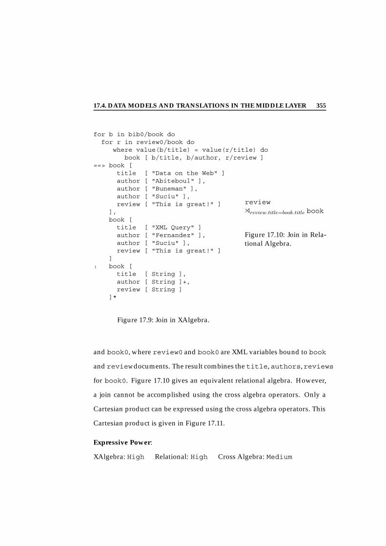
17.4. DATA MODELS AND TRANSLATIONS IN THE MIDDLE LAYER 355
for b in bib0/book dofor r in review0/book do
where value(b/title) = value(r/title) dobook [ b/title, b/author, r/review ]
==> book [title [ "Data on the Web" ]author [ "Abiteboul" ],author [ "Buneman" ],author [ "Suciu" ],review [ "This is great!" ]
],book [
title [ "XML Query" ]author [ "Fernandez" ],author [ "Suciu" ],review [ "This is great!" ]
]: book [
title [ String ],author [ String ]+,review [ String ]
]*
Figure 17.9: Join in XAlgebra.
review1review.title=book.title book
Figure 17.10: Join in Rela-tional Algebra.
and book0, where review0 and book0 are XML variables bound to book
and reviewdocuments. The result combines the title,authors,reviews
for book0. Figure 17.10 gives an equivalent relational algebra. However,
a join cannot be accomplished using the cross algebra operators. Only a
Cartesian product can be expressed using the cross algebra operators. This
Cartesian product is given in Figure 17.11.
Expressive Power:
XAlgebra: High Relational: High Cross Algebra: Medium

17.4. DATA MODELS AND TRANSLATIONS IN THE MIDDLE LAYER 356
CAG = CT1 Æ CT2 Æ CT3 Æ CT4
where CT1 = e10:<book0,author0>(e1:< book, author >), (author0(author) Æbook0(book))
CT2 = e20:<book0,title0>(e2:< book, title >), (title0(title) Æ book0(book) )
CT3 = e30:<book0,reviews.title0>(e3:< reviews.book, reviews.title >),(review.title0 (reviews.title) Æ book0(reviews.book) )
CT4 = e40:<book0,reviews.review0>(e4:< reviews.book, reviews.review >),(reviews.review0 (reviews.review) Æ book0(reviews.book))
Figure 17.11: Join in Cross Algebra.
Other Operators. In addition to the algebra operators that we have pre-
sented here, the XAlgebra also provides the following operators: selection,
quantification, grouping, aggregation, functions and structural recursion.
The operators selection, quantification, aggregation and grouping have an
equivalent relational algebra expression, albeit on the relational model that
does not have the XML supported nested structure. These operators do not
have an equivalent in the cross algebra. Conversely, the cross algebra in-
cludes the subdivide operator which does not have an equivalent in either
the XAlgebra or the relational algebra. However, we believe the XAlgebra
can be easily extended to include the subdivide operator. Another observa-
tion that we have made is that a select operator would greatly enhance the
re-structuring capabilities of the cross algebra. This is we believe a simple
extension of the cross algebra.
17.4. DATA MODELS AND TRANSLATIONS IN THE MIDDLE LAYER 357
Criteria 2: Minimality of Operators
In this category, we explore the minimality of the re-structuring algebra
operators. As can be seen by the examples given in Figures 17.3, 17.6,
17.9, there are no XAlgebra operators that provide “minimal semantics”.
For example, the simplest operation in XAlgebra, projection is a complex
operation that can be broken down into a selection and projection in the
relational algebra. We believe that a minimal semantics algebra operation
set has not been identified for the XAlgebra. On the other hand, for both the
relational and the cross algebra, the operators are defined to have minimal
semantics.
Minimality of Operators:
XAlgebra: Low Relational: High Cross Algebra: High
Criteria 3: Composition Capabilities
A key component for all algebras is the composition of larger expressions
based on the set of algebra operators. All algebras provide this composition
to varying degrees. XAlgebra provides nesting of expressions. Similarly,
relational algebra and the cross algebra also provide nesting of their oper-
ators. In addition, the cross algebra provides a dependency composition,
context dependency, that allows a grouping of operators that have some ex-
ecution dependency and the outputs of all of which are represented in the
final output. Their is no equivalent composition in the relational algebra
and the XAlgebra.
17.4. DATA MODELS AND TRANSLATIONS IN THE MIDDLE LAYER 358
Composition Capabilities:
XAlgebra: Medium Relational: Medium Cross Algebra: High
Summary
To summarize, from a technical standpoint, we believe that for re-struct-
uring in the middle-layer, there are no clear cut winners. Each algebra
has its advantages and disadvantages. In terms of re-structuring expres-
sive power and minimality of operators, the relational algebra is the most
complete and stable. Similar to the relational algebra, the cross algebra
offers a powerful and complete4 set of operators for transformations and
re-structuring. Moreover, the cross algebra operators are minimal and pro-
vide easy composition of larger expressions for complete schema transfor-
mations. However, it would be greatly enhanced if we were to add the select
operator. In contrast, while the XAlgebra is powerful in terms of expressive
power, it falls short on the minimality.
From a practical standpoint, however, the cross algebra lacks the query-
ing capabilities provided by the XAlgebra and the relational algebra. One
of our conclusions from Section 17.4.1 is that XML-Schema is probably the
best practical choice for the middle-layer data model. Based on this, we
would concede that the use of the XAlgebra as the middle layer translation
system may perhaps be the most practical choice as well. However, we
believe that the re-structuring operators of XAlgebra need to be re-worked
4While we do not show the completeness of the cross algebra, this result follows fromsimilar results in the graph linear transformation theory [GY98].

17.4. DATA MODELS AND TRANSLATIONS IN THE MIDDLE LAYER 359
with the addition of the subdivide operator, and with minimality in mind;
and perhaps a marriage of the cross-algebra and the XAlgebra is worth-
while exploration for a future middle-layer mapping algebra.
In conclusion here, we would like to re-iterate that the cross algebra
was designed to provide modeling of transformation in the middle-layer.
Towards that end we have provided a set of modeling primitives, the cross
algebra, the semantics associated with each operator and one explicit mech-
anism to execute these operators. The cross algebra is based on the graph
linear transformation theory, which has shown that these operations are
complete with respect to linear transformations [GY98]. With the above
comparison we have shown that many of these cross algebra expressions
can be easily expressed in current query algebras such as the relational and
the XAlgebra. Thus, for execution purposes the cross algebra expressions
can be expressed as relational or XAlgebra expressions.

17.4. DATA MODELS AND TRANSLATIONS IN THE MIDDLE LAYER 360

361
Part IV
Conclusions and Future Work


363
Chapter 18
Conclusions and Future Work
A key aspect of any persistent information is the simple fact that it changes.
Managing change, which includes the specification and optimization of
change as well the maintenance of any derived information, has been an
important area of research. Today, for every data model there exists a well-
defined set of change primitives [BKKK87, FFM+95, SKC+01] that can al-
ter both the structure (the schema) and the data. Several proposals also
exist for incrementally propagating this primitive change to any derived
information (or view) [ZGMHW95, GB95, RLN97a]. However, this exist-
ing support is lacking in two ways. First, change primitives as presented
in literature are very limiting in terms of their capabilities allowing users to
simply add or remove schema elements. More complex types of changes
such the merging or splitting of schema elements are not not supported in
a principled manner. Secondly, algorithms for maintaining derived infor-
mation often do not account for the potential heterogeneity between the
source and the target. The goal of this dissertation is to provide solutions
18.1. CONTRIBUTIONS OF THIS DISSERTATION 364
that address these two key issues.
18.1 Contributions of this Dissertation
18.1.1 Support for Complex Changes
Support for complex changes in databases exists in the form of pre-defined
set of change operations that can be invoked for different parameters [Bre96,
Ler00]. This work [Bre96, Ler00] defines a set of high-level primitives such
as merge, split and inline for object-oriented databases, in particular for O2.
However, it is difficult to a-priori define (1) all possible complex opera-
tions; and (2) all the possible semantics for the set of complex operations.
For example, a merge of two classes can be accomplished by combining the
attributes and the extents of the two classes, or by forming a new class
that contains only the common set of attributes for the two classes. For
any change beyond the pre-defined set, a user must therefore write pro-
grams that allow him or her to manipulate the structure of their database
as desired. Such an approach is error-prone, provides no guarantees for
consistency of the database, does not lend itself to any kind of verification
or optimization, and is not portable from one database to another.
In Part II of this dissertation, we have have identified the fundamental
components of any complex change - the change expressed in terms of a
set of primitive changes and the corresponding, potentially complex, data
changes. Based on this hypothesis, we have developed SERF [CJR98c] -
an extensible and re-usable framework for schema evolution. The frame-
work is extensible in that the user is not limited to a fixed set of change

18.1. CONTRIBUTIONS OF THIS DISSERTATION 365
primitives. Instead, a user can define their own set of schema changes us-
ing a combination of schema evolution primitives and query language, in
our case OQL (Object Query Language). Any complex change defined by
the user can be stored in the system (SERF system) as a template for sim-
ilar changes by other users. We have developed a prototype of the SERF
system, OQL-SERF, that is defined as a thin-layer on top of existing OODB
systems. We have utilized PSE (Persistent Storage Engine) [O’B97] as our
OODB system.
As noted earlier one of the key advantages of such a framework over
ad-hoc user programs, is the system’s guarantee for consistency of database
post-execution of the complex change. To facilitate this, we consider two
types of consistency - user-level and system-level. A system-level consis-
tency guarantees that all invariants of the data model will be preserved
after the execution of a complex change. We have formally shown that this
system-level consistency is indeed guaranteed by the SERF system [CRed].
A user-level consistency guarantees that a user contract is satisfied after the
execution of a change. To facilitate this, we have developed the notion of
contracts, a set of pre- and post- conditions, that can be defined for a SERF
template [CRH01]. The pre-conditions are verified prior to the execution
of the template and the post-conditions are validated after the template
execution. The template is aborted (transaction is rolled back) if the post-
conditions are not met.
Another area that we have explored in the context of this work is the
optimization of schema evolution operations. Clearly, schema evolution is
a very expensive operation and this expense is exaggerated by the now
18.1. CONTRIBUTIONS OF THIS DISSERTATION 366
more complex changes. We have pursued two approaches for optimiz-
ing this expense: (1) by the reduction of the schema evolution operations
based on some heuristics [CRH00a]; and (2) by reducing the opportunity
for roll-backs or aborted templates [CRH01]. In this dissertation, we have
presented both of these optimization techniques in Chapters 6.1 and 5.3.
To validate the SERF framework and the main concepts behind it, we
have represented numerous complex changes presented in literature as
SERF templates and have validated them using our prototype system
[RCL+99, CJR98c, CJR98a]. Moreover, we have extended the basic concepts
of the SERF framework to also address complex schema evolution oper-
ations that involve relationships between two or more classes [CRH00b].
We have further validated the SERF framework by its application to Web
re-structuring [CCR00, RCC00].
18.1.2 Maintenance of Heterogeneous Views
Views and maintenance of views with respect to source changes has been
a lively topic in database research [ZGMHW95, GB95]. Much of the work
in this area has been based on the assumption that both the source and
the view are defined within the confines of the same data model, and of-
ten within the same database. However, today this world is fast chang-
ing. Today many application engineers struggle to not only publish their
relational, object or ASCII file data on the Web but to also integrate infor-
mation from diverse sources. However, current information integration
technology has moved away from traditional algebra-based views to static
a-priori algorithms. Consequently, maintenance in such scenarios is also

18.1. CONTRIBUTIONS OF THIS DISSERTATION 367
limited to static a-priori algorithms [TIHW01] that rely on the underlying
translation algorithm between the two data models, in this case XML and
relational data model. Such an approach is not extensible to any new trans-
lation technique, a new view, between the same two data models, much
less a different pair of data models. To meet the needs of information inte-
gration and its subsequent maintenance for the future, we consider current
technology in-adequate.
In Part III of this dissertation, we address this problem using a two-
pronged approach. We first define an algebra, a cross algebra, that can
define views such that there is no restriction that forces the view and the
source data models to be the same. To accomplish this, we have defined
the cross algebra that covers the class of linear transformations [GY98] ap-
plied to a graph (Sangam graph) that represents schemas from different
data models. To enable the translation of an entire schema in one data
model to a schema in another data model, we also allow the composition
of these algebra operators by the traditional derivation composition as well
as by our context dependency composition. In the context of this work, we
present the evaluation algorithm for executing a cross algebra expression
and we show that the evaluation algorithm (1) terminates, and (2) it pro-
duces a valid output.
To validate our proposed ideas of cross algebra we have implemented
a prototype system and conducted several experiments that (1) validate in
practice that we are indeed able to express a variety of translation algo-
rithms. We have tested this on the different translation algorithms found in
literature [ZLMR01, FK99, SHT+99, CFLM00, SYU99]; and (2) give a mea-

18.2. FUTURE DIRECTIONS 368
sure of the performance of the prototype system. In this dissertation, we
report these results. All our tests were conducted on the relational and the
XML data models.
Based on the cross algebra operators (and graphs), we have also devel-
oped an incremental update propagation algorithm, Gen Propagation , that
allows us to propagate a change, schema or data change, from the source
to the target. We have shown that this incremental propagation algorithm
produces the same result as complete re-computation. Furthermore, we
have experimentally measured the performance gains that can be achieved
using the incremental propagation algorithm. A key advantage to this al-
gorithm is that it is not tied to any particular translation algorithm between
two data models nor is it tied to any two particular data models. To vali-
date this we have applied this algorithm to propagate changes from XML
to relational database, where the XML documents have been mapped to
the relational data using (a) basic inlining [STZ+99]; (b) shared inlining
[STZ+99]; and (c) ident. In this dissertation, we report on this algorithm
and on our results, both formal and experimental.
18.2 Future Directions
18.2.1 Optimization of Schema Evolution
As noted earlier, schema evolution is a very expensive process. To en-
able dynamic or on-line evolution we must try to reduce the down-time/
unavailability of the system. Researchers have looked at improving sys-
tem availability during schema evolution by proposing execution strate-

18.2. FUTURE DIRECTIONS 369
gies such as deferred execution [Tec94, FMZ94b]. Kahler et al. [KR87] have
looked at pre-execution optimization for reducing the number of update
messages that are sent to maintain replicated sites in the context of dis-
tributed databases. We take a similar approach (merge, cancel, eliminate)
for optimizing a sequence of schema evolution operations. To the best of
our knowledge ours is the first effort to provide an optimization strategy
for a sequence of changes prior to execution a la Kahler [KR87]. However,
while applying this work in the context of SERF templates we neverthe-
less limit our work to dealing with pure schema evolution sequences. That
is, we do not consider the presence of OQL queries which are an essen-
tial component of SERF templates. The heuristics presented here must be
re-examined now in the presence of OQL queries. One idea would be to
combine traditional query optimization techniques with the heuristics for
reducing the schema evolution sequences to enable a more global optimiza-
tion of SERF templates.
Another venue for optimization that we have not examined is the use
of the optimization heuristics together with the lazy or deferred update
techniques proposed by Zicari et al. [FMZ94b]. The deferred update ap-
proach applies updates during query evaluation. That is, when a data set
is requested, if there are any updates applicable to the data set, then the
update is applied before presenting the data set to the user. With a large
data set and a large number of updates, this can potentially cause poor
query response times. A possible optimization here could be the utiliza-
tion of our optimization heuristics to reduce the number of evolution oper-
ations/updates that are applied to the data set.

18.2. FUTURE DIRECTIONS 370
18.2.2 Integrating the Cross Algebra With Existing Local Algebra
One of the limitations of the cross algebra is that it is currently deployable
only as a middle-layer algebra. That is, it is a stand-alone algebra and is not
integrated with any existing algebras such as the relational algebra or XML
algebra. A very interesting future direction would be incorporate the cross
algebra as an extension to SQL and hence the relational algebra. The bind-
ing of the cross algebra to a data model, XML for example, would enable
relational results to be represented as XML documents. Conversely, incor-
porating the cross algebra1 with the XML algebra would enable relational
outputs to be produced by the querying of XML documents.
The potential gains of such an approach are immense. Traditional query
optimization (for relational or XML for example) can be extended to now
incorporate the cross algebra operators. For example, to produce a sorted
relational output from XML documents, it may be more efficient to pipeline
the cross algebra operators and the sort operator on the XML documents,
rather than first sorting the XML data and then translating it to relational
tables. Query translation techniques can also be made more seamless with
such an integration of the cross algebra and the local algebra (XML or rela-
tional).
A key assumption for our propagation algorithm is the fact that a change
is made to the source (relational or XML) and then propagated to the target
(relational or XML). We do not consider the fact that the relational source
for example may itself be a view defined over multiple relational sources.
1If the algebra was bound to the relational model.
18.2. FUTURE DIRECTIONS 371
In such a scenario, a more efficient propagation algorithm would incorpo-
rate existing propagation algorithms for relational views with the propa-
gation algorithm, Gen Propagation that we have developed here. Such an
incorporation is possible only if we are able to integrate the cross algebra
with the local algebra.
Finally, another possible extension to this dissertation is the merging of
the capabilities presented in Parts II and III. In Part II we have focused
on specifying complex change within one data model. In Part III we focus
our efforts on propagating simple changes across data model boundaries.
A possible extension of our work is now possibly propagating complex
changes, a la SERF, through the cross algebra. One solution to this could
lie in the simplification of the problem achieved by perhaps integrating the
cross and the local algebra.
18.2.3 Inverse Update Propagation
In large enterprise systems, information is often dispersed over multiple-
tiers in a combination of physical (source) and virtual (view) databases in
an effort to service a large community of users. Design systems are an ex-
ample of large-scale systems that have to service the needs of many users,
often hundreds of users [PMD95]. In [PMD95], MacKellar and Peckham
describe how a large-scale design is decomposed into a number of special-
ized tasks each requiring its own representation of the design. Users often
specialize in one aspect of the design and thus only deal with one represen-
tation of the design, also termed a perspective or a view. In such large often
multi-tier systems, views (virtual databases) are built upon either another

18.2. FUTURE DIRECTIONS 372
tier of derived information or directly upon the source database systems.
From a user’s perspective there is no distinction between the view that they
work on and the source(s) in the sense of the services and support they ex-
pect for the system. To provide this transparency to the user we need to
effectively support views as first-class citizens [RS99a] and handle execution
of all types of changes seamlessly. Today most database systems provide
support for views but limit them to read-only access or at best allow data
updates [RS99b]. This problem is further amplified when you take into
consideration the fact that the tiers may potentially exist in different data
models.
A possible extension of this dissertation is to now enable inverse prop-
agation of changes, i.e., propagate changes from the view (target) to the
source. A first step to this work could be the propagation of simple change
within the cross algebra with potential extensions to an integrated algebra
(combination of cross and local algebra), and more complex changes.
373
Appendix A
DTDs Used in Experiments
Figure A.1 gives the complete auction.dtd. Figures A.5 and A.6 present
the personal.dtd and play.dtd respectively.

APPENDIX A. DTDS USED IN EXPERIMENTS 374
<!-- DTD for auction database --><!-- $Id: auction.dtd,v 1.15 2001/01/2921:42:35 albrecht Exp $ -->
<!ELEMENT site (regions, categories,catgraph, people,open_auctions,closed_auctions)>
<!ELEMENT categories (category+)><!ELEMENT category (name, description)><!ATTLIST category id ID #REQUIRED><!ELEMENT name (#PCDATA)><!ELEMENT description (text | parlist)><!ELEMENT text (#PCDATA | bold
| keyword | emph)*><!ELEMENT bold (#PCDATA | bold
| keyword | emph)*><!ELEMENT keyword (#PCDATA | bold
| keyword | emph)*><!ELEMENT emph (#PCDATA | bold
| keyword | emph)*><!ELEMENT parlist (listitem)*><!ELEMENT listitem (text | parlist)*><!ELEMENT catgraph (edge*)><!ELEMENT edge EMPTY><!ATTLIST edge from IDREF #REQUIRED to
IDREF #REQUIRED>
Figure A.1: The auction.dtd of the Xmark Benchmark [SWK+01].
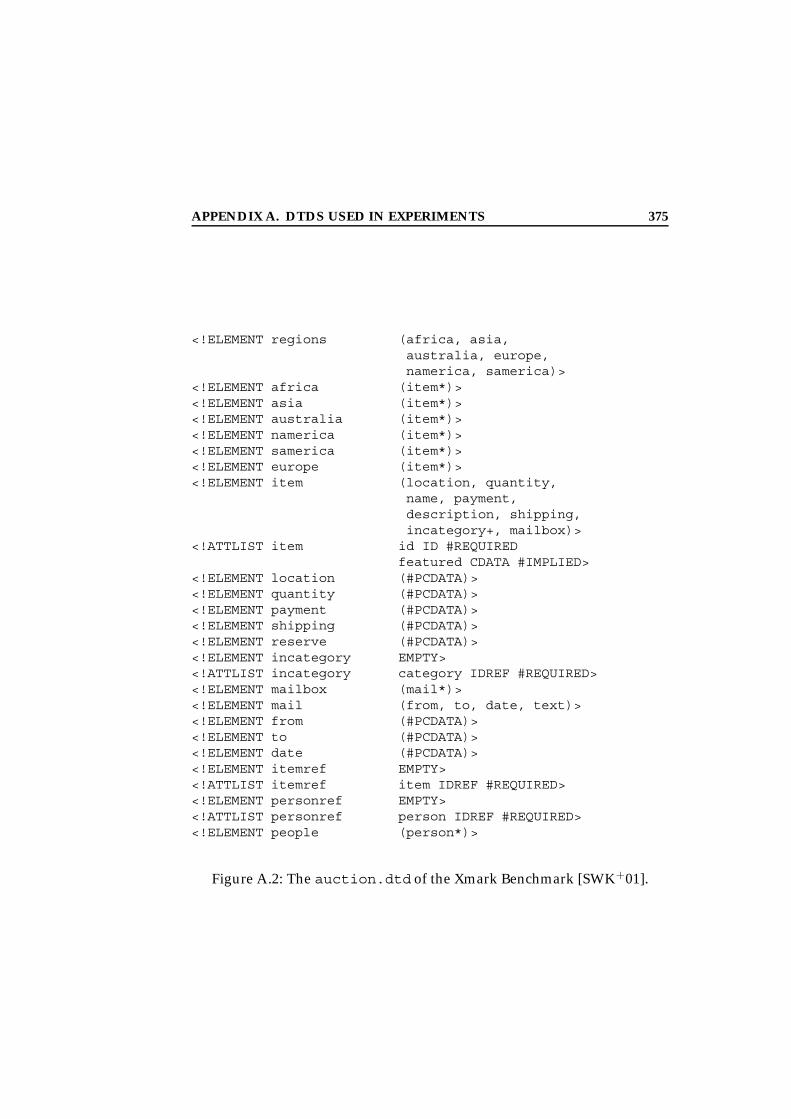
APPENDIX A. DTDS USED IN EXPERIMENTS 375
<!ELEMENT regions (africa, asia,australia, europe,namerica, samerica)>
<!ELEMENT africa (item*)><!ELEMENT asia (item*)><!ELEMENT australia (item*)><!ELEMENT namerica (item*)><!ELEMENT samerica (item*)><!ELEMENT europe (item*)><!ELEMENT item (location, quantity,
name, payment,description, shipping,incategory+, mailbox)>
<!ATTLIST item id ID #REQUIREDfeatured CDATA #IMPLIED>
<!ELEMENT location (#PCDATA)><!ELEMENT quantity (#PCDATA)><!ELEMENT payment (#PCDATA)><!ELEMENT shipping (#PCDATA)><!ELEMENT reserve (#PCDATA)><!ELEMENT incategory EMPTY><!ATTLIST incategory category IDREF #REQUIRED><!ELEMENT mailbox (mail*)><!ELEMENT mail (from, to, date, text)><!ELEMENT from (#PCDATA)><!ELEMENT to (#PCDATA)><!ELEMENT date (#PCDATA)><!ELEMENT itemref EMPTY><!ATTLIST itemref item IDREF #REQUIRED><!ELEMENT personref EMPTY><!ATTLIST personref person IDREF #REQUIRED><!ELEMENT people (person*)>
Figure A.2: The auction.dtd of the Xmark Benchmark [SWK+01].

APPENDIX A. DTDS USED IN EXPERIMENTS 376
<!ELEMENT person (name, emailaddress,phone?, address?,homepage?, creditcard?,profile?, watches?)>
<!ATTLIST person id ID #REQUIRED><!ELEMENT emailaddress (#PCDATA)><!ELEMENT phone (#PCDATA)><!ELEMENT address (street, city, country,
province?, zipcode)><!ELEMENT street (#PCDATA)><!ELEMENT city (#PCDATA)><!ELEMENT province (#PCDATA)><!ELEMENT zipcode (#PCDATA)><!ELEMENT country (#PCDATA)><!ELEMENT homepage (#PCDATA)><!ELEMENT creditcard (#PCDATA)><!ELEMENT profile (interest*, education?,
gender?,business, age?)>
<!ATTLIST profile income CDATA #IMPLIED><!ELEMENT interest EMPTY><!ATTLIST interest category IDREF #REQUIRED><!ELEMENT education (#PCDATA)><!ELEMENT income (#PCDATA)><!ELEMENT gender (#PCDATA)><!ELEMENT business (#PCDATA)><!ELEMENT age (#PCDATA)><!ELEMENT watches (watch*)><!ELEMENT watch EMPTY><!ATTLIST watch open_auction IDREF #REQUIRED><!ELEMENT open_auctions (open_auction*)>
Figure A.3: The auction.dtd of the Xmark Benchmark [SWK+01].
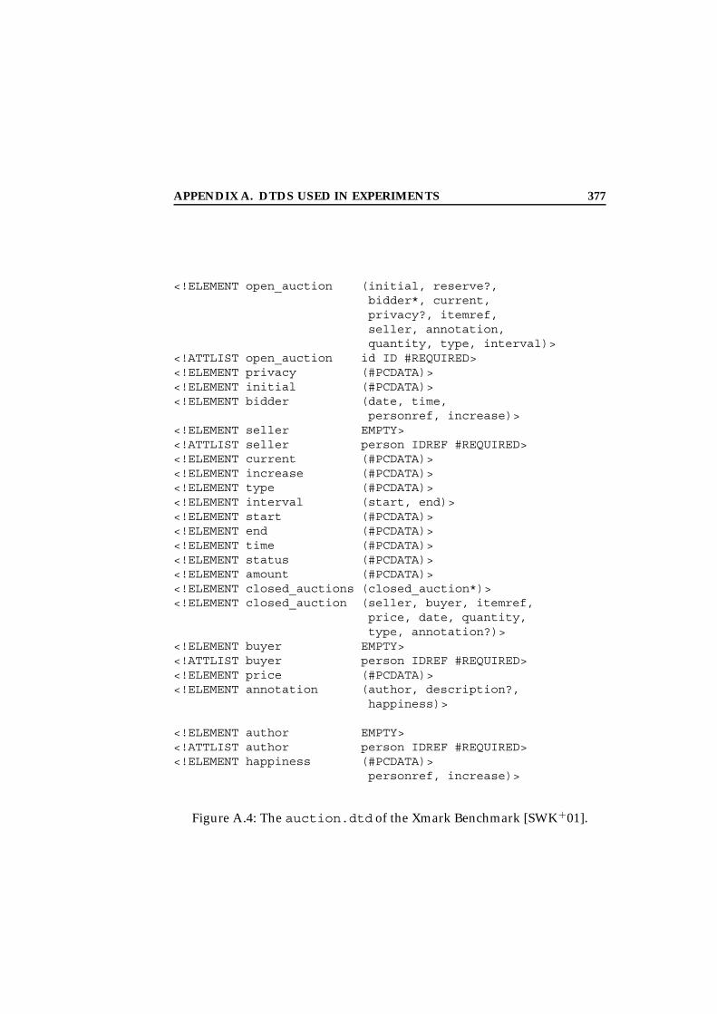
APPENDIX A. DTDS USED IN EXPERIMENTS 377
<!ELEMENT open_auction (initial, reserve?,bidder*, current,privacy?, itemref,seller, annotation,quantity, type, interval)>
<!ATTLIST open_auction id ID #REQUIRED><!ELEMENT privacy (#PCDATA)><!ELEMENT initial (#PCDATA)><!ELEMENT bidder (date, time,
personref, increase)><!ELEMENT seller EMPTY><!ATTLIST seller person IDREF #REQUIRED><!ELEMENT current (#PCDATA)><!ELEMENT increase (#PCDATA)><!ELEMENT type (#PCDATA)><!ELEMENT interval (start, end)><!ELEMENT start (#PCDATA)><!ELEMENT end (#PCDATA)><!ELEMENT time (#PCDATA)><!ELEMENT status (#PCDATA)><!ELEMENT amount (#PCDATA)><!ELEMENT closed_auctions (closed_auction*)><!ELEMENT closed_auction (seller, buyer, itemref,
price, date, quantity,type, annotation?)>
<!ELEMENT buyer EMPTY><!ATTLIST buyer person IDREF #REQUIRED><!ELEMENT price (#PCDATA)><!ELEMENT annotation (author, description?,
happiness)>
<!ELEMENT author EMPTY><!ATTLIST author person IDREF #REQUIRED><!ELEMENT happiness (#PCDATA)>
personref, increase)>
Figure A.4: The auction.dtd of the Xmark Benchmark [SWK+01].

APPENDIX A. DTDS USED IN EXPERIMENTS 378
<?xml encoding="UTF-8"?><!ELEMENT personnel (person)+>
<!ELEMENT person (name,email*,url*,link?)><!ATTLIST person id ID #REQUIRED><!ATTLIST person note CDATA #IMPLIED><!ATTLIST person salary CDATA #IMPLIED>
<!ELEMENT name (family,given)>
<!ELEMENT family (#PCDATA)>
<!ELEMENT given (#PCDATA)>
<!ELEMENT email (#PCDATA)>
<!ELEMENT url EMPTY><!ATTLIST url href CDATA ’http://’>
<!ELEMENT link EMPTY><!ATTLIST link manager IDREF #IMPLIED><!ATTLIST link subordinates IDREFS #IMPLIED>
<!NOTATION gif PUBLIC ’-//APP/Photoshop/4.0’’photoshop.exe’>
Figure A.5: The personal.dtd used for Sangam testing.

APPENDIX A. DTDS USED IN EXPERIMENTS 379
<!-- DTD for Shakespeare J. Bosak 1994.03.01,1997.01.02 -->
<!-- Revised for case sensitivity 1997.09.10 --><!-- Revised for XML 1.0 conformity 1998.01.27(thanks to Eve Maler) -->
<!-- <!ENTITY amp "&#38;"> --><!ELEMENT PLAY (TITLE, FM, PERSONAE, SCNDESCR,
PLAYSUBT, INDUCT?, PROLOGUE?,ACT+, EPILOGUE?)>
<!ELEMENT TITLE (#PCDATA)><!ELEMENT FM (P+)><!ELEMENT P (#PCDATA)><!ELEMENT PERSONAE (TITLE, (PERSONA | PGROUP)+)><!ELEMENT PGROUP (PERSONA+, GRPDESCR)><!ELEMENT PERSONA (#PCDATA)><!ELEMENT GRPDESCR (#PCDATA)><!ELEMENT SCNDESCR (#PCDATA)><!ELEMENT PLAYSUBT (#PCDATA)><!ELEMENT INDUCT (TITLE, SUBTITLE*,
(SCENE+|(SPEECH|STAGEDIR|SUBHEAD)+))><!ELEMENT ACT (TITLE, SUBTITLE*, PROLOGUE?,
SCENE+, EPILOGUE?)><!ELEMENT SCENE (TITLE, SUBTITLE*,
(SPEECH | STAGEDIR | SUBHEAD)+)><!ELEMENT PROLOGUE (TITLE, SUBTITLE*, (STAGEDIR
| SPEECH)+)><!ELEMENT EPILOGUE (TITLE, SUBTITLE*, (STAGEDIR
| SPEECH)+)><!ELEMENT SPEECH (SPEAKER+, (LINE | STAGEDIR
| SUBHEAD)+)><!ELEMENT SPEAKER (#PCDATA)><!ELEMENT LINE (#PCDATA | STAGEDIR)*><!ELEMENT STAGEDIR (#PCDATA)><!ELEMENT SUBTITLE (#PCDATA)><!ELEMENT SUBHEAD (#PCDATA)>
Figure A.6: The play.dtd available with JAXP1.1.

APPENDIX A. DTDS USED IN EXPERIMENTS 380
381
Bibliography
[AH90] T. Andrews and C. Harris. Combining Language andDatabase Advances in an Object-Oriented Development En-vironment. In Readings in Object-Oriented Database Systems,pages 186–196, 1990.
[ANS92] ANSI Standard. The SQL 92 Standard.http://www.ansi.org/, 1992.
[AT96] P. Atzeni and R. Torlone. Management of Multiple Modelsin an Extensible Database Design Tool. In Peter M. G. Apersand et al., editors, Advances in Database Technology - EDBT’96,Avignon, France, March 25-29, LNCS. Springer, 1996.
[AYBS97] S. Amer-Yahia, P. Breche, and C.S.D Santos. Object Viewsand Updates. In ISI, 1997.
[BB99] P.A. Bernstein and T. Bergstraesser. Meta-Data Support forData Transformations Using Microsoft Repository. In IEEEBulletin - Special Issue on Database Tranformation Technology,pages 9–14, 1999.
[BCGMG97] E. Bertino, B. Catania, J. Garcia-Molina, and G. Guerrini. AFormal Model of Views for Object-Oriented Database Sys-tems. Journal of Theory and Practice of Object Systems (TAPOS),1997.
[BCVG86] A. Buchmann, R. Carrera, and M. Vazquez-Galindo. AGeneralized Constraint and Exception Handler for Object-Oriented CAD-DBMS. In Proceedings of the InternationalWorkshop on Object-Oriented Database Systems, pages 38–49,1986.

BIBLIOGRAPHY 382
[Ber92] E. Bertino. A View Mechanism for Object-OrientedDatabases. In 3rd Int. Conference on Extending Database Tech-nology, pages 136–151, March 1992.
[Ber99] Bernstein, P. A. and Bergstraesser, T. et al. Microsoft Reposi-tory Version 2 and the Open Information Model. InformationSystems, 2(24):71–98, 1999.
[BFK95] P. Breche, F. Ferrandina, and M. Kuklok. Simulation ofSchema Change using Views. In Int. Conference and Workshopon Database and Expert Systems Applications, 1995.
[BH93] P.L. Bergstein and W.L Hursch. Maintaining Behavioral Con-sistency during Schema Evolution. In International Sympo-sium on Object Technologies for Advanced Software, pages 176–193, 1993.
[BHJ+96] P.J. Black, K.M. Hall, M.D. Jones, T.N. Larson, and P.J. Wind-ley. A Brief Introduction to Formal Methods. In Proceedingsof CICC, pages 377–380, 1996.
[BK90] F. Bancilhon and W. Kim. Object-Oriented Database Sys-tems: In Transition. In SIGMOD RECORD, volume 19, De-cember 90.
[BKKK87] J. Banerjee, W. Kim, H. J. Kim, and H. F. Korth. Seman-tics and Implementation of Schema Evolution in Object-Oriented Databases. SIGMOD, pages 311–322, 1987.
[BL01] A. Bonifati and D. Lee. Comparative Examples of XMLSchema and Query Languages. In Internet Document, Jan-uary 2001.
[Bla98] P.E. Black. Axiomatic Semantic Verification of a Secure WebServer. PhD thesis, Brigham Young University, February1998.
[BLN86] C. Batini, M. Lenzerini, and S. Navathe. A ComparativeAnalysis of Methedologies for Database Schema Integration.ACM Computing Surveys, 18(4), December 1986.
[BMO+89] R. Bretl, D. Maier, A. Otis, J. Penney, B. Schuchardt, J. Stein,E. H. Williams, and M. Williams. The GemStone Data Man-
BIBLIOGRAPHY 383
agement System. In Object-Oriented Concepts, Databases andApplications, pages 283–308. ACM Press, 1989.
[Boo94] G. Booch. Object-Oriented Analysis and Design. BenjaminCummings Pub., 1994.
[BPSM00] T. Bray, J. Paoli, and C.M. (Eds). Sperberg-McQueen. Extensible Markup Language (XML)1.0.http://www.w3c.org/TR/2000/REC-xml-20001006, Octo-ber 2000.
[BR00] P. A. Bernstein and E. Rahm. Data Warehouse Scenarios forModel Management. In International Conference on ConceptualModeling, 2000.
[Bre96] P. Breche. Advanced Primitives for Changing Schemas ofObject Databases. In Conference on Advanced Information Sys-tems Engineering, pages 476–495, 1996.
[BS81] F. Bancilhon and N. Spyratos. Update Semantics of Re-lational Views. ACM Transactions on Database Systems,6(4):557–575, December 1981.
[CCR00] L. Chen, K.T. Claypool, and E.A Rundensteiner. SERFing theWeb: The Re-Web Approach for Web Re-Structuring. WorldWide Web Journal: Special Issue on World Wide Web Data Man-agement, 2000. Final Revision Submitted Feb. 2000.
[Cea97] R.G.G Cattell and et al. The Object Database Standard: ODMG2.0. Morgan Kaufmann Publishers, Inc., 1997.
[CFLM00] B. Catania, E. Ferrari, A. Levy, and A. Meldelzon. XML andObject Technology. In ECOOP Workshop on XML and ObjectTechnology, LNCS 1964, pages 191–202, 2000.
[CJR98a] K.T. Claypool, J. Jin, and E.A. Rundensteiner. OQL SERF: AnODMG Implementation of the Template-Based Schema Evo-lution Framework. In Centre for Advanced Studies Conference,pages 108–122, November 1998.
[CJR98b] K.T. Claypool, J. Jin, and E.A. Rundensteiner. OQL SERF:An ODMG Implementation of the Template-Based SchemaEvolution Framework. Technical Report WPI-CS-TR-98-14,Worcester Polytechnic Institute, July 1998.

BIBLIOGRAPHY 384
[CJR98c] K.T. Claypool, J. Jin, and E.A. Rundensteiner. SERF: SchemaEvolution through an Extensible, Re-usable and FlexibleFramework. In Int. Conf. on Information and Knowledge Man-agement, pages 314–321, November 1998.
[CJR98d] K.T. Claypool, J. Jin, and E.A. Rundensteiner. SERF:SchemaEvolution through an Extensible, Re-usable and FlexibleFramework. Technical Report WPI-CS-TR-98-9, WorcesterPolytechnic Institute, May 1998.
[Cla92] S.M. Clamen. Type Evolution and Instance Adaptation.Technical Report CMU-CS-92-133R, Carnegie Mellon Uni-versity, School of Computer Science, 1992.
[Clu98] S. Cluet. Designing OQL: Allowing objects to be queried.Journal of Information Systems, 23(5):279–305, 1998.
[CNR99] K.T. Claypool, C. Natarajan, and E.A. Rundensteiner. Op-timizing the Performance of Schema Evolution Sequences.Technical Report WPI-CS-TR-99-06, Worcester PolytechnicInstitute, February 1999.
[CNR00] K.T. Claypool, C. Natarajan, and E.A. Rundensteiner. Opti-mizing the Performance of Schema Evolution Sequences. InECOOP Symposioum on Object Databases, 2000.
[Cor00] Oracle Corporation. Oracle 8i.http://www.oracle.com/ip/deploy/database/8i/index.html,2000.
[CRCK98] K. Claypool, E.A. Rundensteiner, L. Chen, and B. Kothari.Re-usable ODMG-based Templates for Web View Genera-tion and Restructuring. In WIDM’98, pages 314–321, 1998.
[CRH00a] K. T. Claypool, E. A. Rundensteiner, and G.T. Heineman.Evolving the Software of a Schema Evolution System. InNinth International Workshop on Foundations of Models and Lan-guages for Data and Objects, September 2000.
[CRH00b] K. T. Claypool, E. A. Rundensteiner, and G.T. Heineman.ROVER: A Framework for the Evolution of Relationships.In Nineteenth International Conference on Conceptual Modeling,October 2000.

BIBLIOGRAPHY 385
[CRH01] K.T. Claypool, E.A Rundensteiner, and G.T. Heineman.ROVER: Flexible Yet Consistent Evolution of Relationships.Data and Knowledge Engineering, 39(1):27–50, Oct 2001.
[CRed] K.T. Claypool and E.A. Rundensteiner. SERF:Schema Evo-lution through an Extensible, Re-usable and Flexible Frame-work. , submitted.
[CRZ+01] K.T. Claypool, E.A. Rundensteiner, X. Zhang, H. Su,H. Kuno, W-C. Lee, and G. Mitchell. SANGAM: A Solu-tion to Support Multiple Data Models, Their Mappings andMaintenance. In Demo Session Proceedings of SIGMOD’01,2001.
[Day89] U. Dayal. Queries and views in an object-oriented datamodel. In Intern. Work. on Data Base Programming Language 2,1989.
[DB78] U. Dayal and P. Berstein. On the Updatability of RelationalViews. In VLDB, 1978.
[DK97] S.B. Davidson and A.S. Kosky. WOL: A Language forDatabase Transformations and Constraints. In IEEE Int. Conf.on Data Engineering, pages 55–65, 1997.
[DKE94] S.B. Davidson, A.S. Kosky, and B. Eckman. FacilitatingTransformations in a Human Genome Project Database. InInt. Conf. on Information and Knowledge Management, pages423–432, 1994.
[Dmi98] M. Dmitriev. The First Experience of Class Evolution Sup-port in PJama. In Third International Conference on Persistenceand Java, 1998.
[DZ91] C. Delcourt and R. Zicari. The Design of an Integrity Con-sistency Checker (ICC) for an Object Oriented-Database Sys-tem. In P. America, editor, ECOOP, pages 97–117, 1991.
[EN96] Ramez Elmasri and Shamkant B. Navathe. Fundamentalsof Database Systems. The Benjamin/Cummings PublishingCompany, Inc., 1996.
[Fal01] D.C. Fallside. XML Schema 1.1.http://www.w3c.org/TR/xmlschema-0, May 2001.
BIBLIOGRAPHY 386
[FFHI72] J.P. Fry, R.L. Frank, and E.A. Hershey III. A DevelopmentModel for Data Translation. In A. L. Dean., editor, Proceed-ings of 1972 ACM-SIGFIDET Workshop on Data Description,Access and Control, Denver, Colorado, November 29 - December1, 1972, pages 77–105. ACM, 1972.
[FFM+95] F. Ferrandina, G. Ferran, T. Meyer, J. Madec, and R. Zicari.Schema and Database Evolution in the O2 Object DatabaseSystem. In Int. Conference on Very Large Data Bases, 1995.
[FFM+01a] P. Fankhauser, M. Fernandez, A. Malhotra, M. a Rys,J. Simeon, and P. Wadler. XQuery 1.0 Formal Seman-tics. http://www.w3c.org/TR/2001/query-semantics, June2001.
[FFM+01b] P. Fankhauser, M. Fernandez, A. Malhotra, M. a Rys,J. Simeon, and P. Wadler. XQuery 1.0 Formal Semantics.http://www.w3c.org/TR/2001/query-semantics, Novem-ber 2001.
[FK99] D. Florescu and D. Kossmann. Storing and Querying XMLData Using an RDBMS. In Bulletin of the Technical Committeeon Data Engineering, pages 27–34, Sept. 1999.
[FMZ94a] F. Ferrandina, T. Meyer, and R. Zicari. Correctness of LazyDatabase Updates for an Object Database System. In Proc. ofthe 6th Int’l Workshop on Persistent Object Systems, 1994.
[FMZ94b] F. Ferrandina, T. Meyer, and R. Zicari. Implementing LazyDatabase Updates for an Object Database System. In VLDB,pages 261–272, 1994.
[FSS+97] C. Faloutsos, R.T. Snodgrass, V.S. Subrahmanian, S. Zaniolo,C. Ceri, and R. Zicari. Advanced Database Systems. MorganKaufmann, 1997.
[GB95] A. Gupta and J.A. Blakeley. Using Partial Information to Up-date Materialized Views. Information Systems, 20(8):641–662,1995.
[GGMS97] D. Gluche, T. Grust, C. Mainberger, and M.H. Scholl. Incre-mental Updates for Materialized OQL Views. In Proceedingsof the Fifth DOOD Conference, pages 52–66, December 1997.

BIBLIOGRAPHY 387
[GM93] M.J.C Gordon and T.F. Melham. Introduction to HOL: A The-orem Proving Environment for Higher Order Logic, 1993.
[GSW95] Y. Gurevich, N. Soparkar, and C. Wallace. Formalizingdatabase recovery. In COMAD, 1995.
[GY98] J. Gross and J. Yellen. Graph Theory and it Applications. CRCPress, 1998.
[Har94] C. Harrison. An Adaptive Query Language for Object-Oriented Databases: Automatic Navigation Through Par-tially Specified Data Structures. Master’s thesis, NorthEast-ern University, June 1994.
[HD91] M. Hardwick and B. R. Downie. On object-orienteddatabases, materialized views, and concurrent engineering.In Proceedings of the 1991 ASME Int. Computers for EngineeringConference and Exposition. Engineering Databases: An Engi-neering Resource, 1991.
[HMN+99] L.M. Haas, R.J. Miller, B. Niswonger, M.T. Roth, P. Schwarz,and E.L. Wimmers. Transforming Heterogeneous Data withDatabase Middleware: Beyond Integration. IEEE Data Engi-neering Bulletin, 22(1):31–36, 1999.
[HP00] H. Hosoya and B.C. Pierce. XDuce: A Typed XML ProcessingLanguage. In WebDB(Informal Proceedings), pages 111–116.ACM Press, 2000.
[HS96] W.L. Hursch and L.M. Seiter. Automating the Evolution ofObject-Oriented Systems. In International Symposium on Ob-ject Technologies for Advanced Software, pages 2–21, Kanazawa,Japan, March 1996. Springer Verlag, Lecture Notes in Com-puter Science.
[IBM98] IBM Alphaworks. An Experimental Implementa-tion of the Construction Rules sect ion of the XSL.http://www.alphaworks.ibm.com/tech/LotusXSL, 1998.
[Inc93] Itasca Systems Inc. Itasca Systems Technical Report. Techni-cal Report TM-92-001, OODBMS Feature Checklist. Rev 1.1,Itasca Systems, Inc., December 1993.

BIBLIOGRAPHY 388
[Jav96] JavaCC. http://www.sun.com/suntest/JavaCC/, 1996.
[Jin98] J. Jin. An Extensible Schema Evolution Framework forObject-Oriented Databases using OQL. Master’s thesis,Worcester Polytechnic Institute, May 1998.
[Kau98] Rajesh Kaushal. View-based support for transparent schemaevolution in federated database systems. In InternationalWorkshop on. Issues and Applications of Database Technology,1998.
[KC88] W. Kim and H. Chou. Versions of Schema For OODBs. InProc. 14th VLDB, pages 148–159, 1988.
[KC90] R. H. Katz and E. Chang. Managing change in a computer-aided design database. In S. B. Zdonik and D. Maier, editors,Readings in Object-Oriented Database Systems, pages 400–407.Morgan Kaufmann Pub., 1990.
[Kel82] A. Keller. Updates to Relational Database Through ViewsInvolving Joins. In Scheuermann, 1982.
[KGBW90] W. Kim, J. F. Garza, N. Ballou, and D. Woelk. Architecture ofthe ORION Next-Generation Database System. IEEE Trans-actions on Knowledge and Data Engineering, 2(1), March 1990.
[KKS92] M. Kifer, W. Kim, and Y. Sagiv. Querying Object-OrientedDatabases. SIGMOD, pages 393–402, 1992.
[KL95] G. Koch and K. Loney. Oracle: The Complete Reference. OraclePress, Osborne-McGraw Hill, 1995.
[KR87] Bo Kahler and Oddvar Risnes. Extending logging fordatabase snapshot refresh. In Peter M. Stocker, William Kent,and Peter Hammersley, editors, VLDB’87, Proceedings of 13thInternational Conference on Very Large Data Bases, September1-4, 1987, Brighton, England, pages 389–398. Morgan Kauf-mann, 1987.
[KR98] H. A. Kuno and E. A. Rundensteiner. Incremental Mainte-nance of Materialized Views in OODBs. IEEE Transaction onData and Knowledge Engineering,, 1998.

BIBLIOGRAPHY 389
[KR02] A. Koeller and E.A. Rundensteiner. Incremental Mainte-nance of Schema-Restructuring Views. In Int. Conference onExtending Database Technology (EDBT), page to appear, 2002.
[Lau96] S.-E. Lautemann. An Introduction to Schema Versioning inOODBMS. In Int. Conference and Workshop on Database andExpert Systems Applications, pages 132–139, 1996.
[Lau97a] S.-E. Lautemann. A Propagation Mechanism for PopulatedSchema Versions. In IEEE Int. Conf. on Data Engineering,pages 67–78, 1997.
[Lau97b] S.-E. Lautemann. Schema Versions in Object-OrientedDatabase Systems. In Int. Conference on Database Systems forAdvanced Applications (DASFAA), pages 323–332, 1997.
[Ler96] B.S. Lerner. A Model for Compound Type Changes Encoun-tered in Schema Evolution. Technical Report UM-CS-96-044,University of Massachusetts, Amherst, 1996.
[Ler00] B.S. Lerner. A Model for Compound Type Changes Encoun-tered in Schema Evolution. ACM Transactions on DatabaseSystems, 25(1):83–127, 2000.
[LLPS91] G. Lohman, B. Lindsay, H. Pirahesh, and K.B. Schiefer. Ex-tensions to StarBurst: Objects, Types and Rules. Communica-tions of the ACM, 34(10):95–109, 1991.
[LSS96] L.V.S. Lakshmanan, F. Sadri, and I.N Subramanian.SchemaSQL - A Language for Interoperability in RelationalMulti-database Systems. In vldb, 1996.
[LZLH94] L. Liu, R. Zicari, K. Lieberherr, and W. Hursch. Polymor-phic reuse mechanisms for object-oriented database specifi-cations. In Ahmed K. Elmagarmid and Erich Neuhold, ed-itors, Proceedings of the 10th International Conference on DataEngineering, pages 180–189, Houston, TX, February 1994.IEEE Computer Society Press.
[Mey92] B. Meyer. Applying “Design By Contract”. IEEE Computer,25(10):20–32, 1992.

BIBLIOGRAPHY 390
[MIR93] R. J. Miller, Y. E. Ioannidis, and R. Ramakrishnan. The Useof Information Capacity in Schema Integration and Transla-tion. In Int. Conference on Very Large Data Bases, pages 120–133, 1993.
[MNJ94] M.A Morsi, S. Navathe, and Shilling J. On BehavioralSchema Evolution in Object-Oriented-Database System. InInt. Conference on Extending Database Technology (EDBT),pages 173–186, 1994.
[MR83] L. Mark and N. Roussopoulos. Integration of Data, Schemaand Meta-Schema in the Context of Self-Documenting DataModels. In Carl G. Davis, Sushil Jajodia, Peter A. Ng, andRaymond T. Yeh, editors, Proceedings of the 3rd Int. Conf. onEntity-Relationship Approach (ER’83), pages 585–602. NorthHolland, 1983.
[MS93] S. Monk and I. Sommerville. Schema Evolution in OODBsUsing Class Versioning. In SIGMOD RECORD, VOL. 22,NO.3, September 1993.
[MZ98] T. Milo and S. Zohar. Using Schema Matching to SimplifyHeterogeneous Data Translation. In Ashish Gupta, OdedShmueli, and Jennifer Widom, editors, VLDB’98, Proceedingsof 24rd International Conference on Very Large Data Bases, Au-gust 24-27, 1998, New York City, New York, USA, pages 122–133. Morgan Kaufmann, 1998.
[NACP01] B. Nguyen, S. Abiteboul, G. Cobena, and M. Preda. Moni-toring XML data on the Web. In Proceedings of the ACM SIG-MOD International Conference on Mana gement of Data, SantaBarbara, CA, pages 437–448, May 2001.
[NLR98] A. Nica, A. J. Lee, and E. A. Rundensteiner. The CVS Algo-rithm for View Synchronization in Evolvable Large-Scale In-formation Systems. In Proceedings of International Conferenceon Extending Database Technology (EDBT’98), pages 359–373,Valencia, Spain, March 1998.
[O’B97] P. O’Brien. Making Java Objects Persistent. Java Report,1(1):49–60, 1997.
BIBLIOGRAPHY 391
[Obj93] Object Design Inc. ObjectStore - User Guide: DML. ObjectStoreRelease 3.0 for UNIX Systems. Object Design Inc., December1993.
[OPS+95] M.T. Oszu, R. J. Peters, D. Szafron, B. Irani, A. Lipka, andA. Munoz. TIGUKAT: A Uniform Behavioral ObjectbaseManagement System. VLDB Journal, 4:100–147, 1995.
[ORS92] S. Owre, J.M. Rushby, and N. Shankar. PVS: A PrototypeVerification System. In 11th CADE, Lecture Notes in ArtificialIntelligence, pages 748–752, 1992.
[PMD95] Joan Peckham, Bonnie MacKellar, and Michael Doherty.Data model for extensible support of explicit relationshipsin design databases. VLDB Journal, 4(2):157–191, 1995.
[PO95] R.J. Peters and M.T. Ozsu. Axiomatization of DynamicSchema Evolution in Objectbases. In IEEE Int. Conf. on DataEngineering, pages 156–164, 1995.
[PR95] M.P. Papazoglou and N. Russell. A Semantic Meta-ModelingApproach to Schema Transformation. In CIKM ’95, pages113–121. ACM, 1995.
[QCR00] L.P. Quan, L. Chen, and E. A. Rundensteiner. Argos: EfficientRefresh in an XQL-Based Web Caching System. In WebDB,Dallas, Taxas, pages 23–28, May 2000.
[RAJB00] J. Roddick, L. Al-Jadir, and L.and et al. Bertossi. Evolutionand Change in Data Management - Issues and Directions.SIGMOD Record, 29(1):21–26, March 2000.
[RCC00] E.A. Rundensteiner, K.T. Claypool, and L. et. al Chen. SERF-ing the Web: A Comprehensive Approach for Web Site Man-agement. In Demo Session Proceedings of SIGMOD’00, 2000.
[RCL+99] E.A. Rundensteiner, K.T. Claypool, M. Li, L. Chen, X. Zhang,C. Natarajan, J. Jin, S. De Lima, and S. Weiner. SERF: ODMG-Based Generic Re-structuring Facility. In Demo Session Pro-ceedings of SIGMOD’99, pages 568–570, 1999.
[RLN97a] E. A. Rundensteiner, A. J. Lee, and A. Nica. On Preserv-ing Views in Evolving Environments. In Proceedings of 4th

BIBLIOGRAPHY 392
Int. Workshop on Knowledge Representation Meets Databases(KRDB’97): Intelligent Access to Heterogeneous Information,pages 13.1–13.11, Athens, Greece, August 1997.
[RLN97b] E. A. Rundensteiner, A. J. Lee, and A. Nica. On Preserv-ing Views in Evolving Environments. In Proceedings of 4thInt. Workshop on Knowledge Representation Meets Databases(KRDB’97): Intelligent Access to Heterogeneous Information,pages 13.1–13.11, Athens, Greece, August 1997.
[RLR98] E.A. Rundensteiner, A. Lee, and Y.-G. Ra. Capacity-Augmenting Schema Changes on Object-OrientedDatabases: Towards Increased Interoperability. In Object-Oriented Information Systems, 1998.
[Roc00] Rochade Information Model. Rochade Information Model.http://support.viasoft.com/html/2RochDocDownload.html,2000.
[RR87] A. Rosenthal and D. Reiner. Theoretically Sound Trans-formations for Practical Database Design. In Salvatore T.March, editor, Entity-Relationship Approach, Proceedings of theSixth International Conference on Entity-Relationship Approach,New York, USA, November 9-11, 1987, pages 115–131, 1987.
[RR94] Y. G. Ra and E. A. Rundensteiner. A Transparent Object-Oriented Schema Change Approach Using View SchemaEvolution. Technical Report CSE-TR-211-94, University ofMichigan, 1994.
[RR97] Y. G. Ra and E. A. Rundensteiner. A Transparent SchemaEvolution System Based on Object-Oriented View Technol-ogy. IEEE Transactions on Knowledge and Data Engineering,9(4):600–624, September 1997.
[RS99a] A. Rosenthal and E. Sciore. First-class views: A key to user-centered computing. In SIGMOD, pages 29–36, May 1999.
[RS99b] A. Rosenthal and E. Sciore. First-Class Views: A Key to User-Centered Computing. SIGMOD Record, 28(3):29–36, May1999.

BIBLIOGRAPHY 393
[Run92] E. A. Rundensteiner. MultiView: Methodology for Support-ing Multiple Views in Object-Oriented Databases”. In 18thVLDB Conference, pages 187–198, 1992.
[RW98] J.V.E. Ridgeway and J.C Wileden. Towards Class Evolutionin Persistent Java. In Third International Conference on Persis-tence and Java, 1998.
[San95] C. S. Santos. Design and Implementation of Object-OrientedViews. In Int. Conference and Workshop on Database and ExpertSystems Applications, pages 91–102, 1995.
[SCR00] H. Su, K. T. Claypool, and E. A. Rundensteiner. Extendingthe Object Query Language for Transparent Meta-Data Ac-cess. In Ninth International Workshop on Foundations of Modelsand Languages for Data and Objects, September 2000.
[SHL75] Nan C. Shu, Barron C. Housel, and Vincent Y. Lum. Convert:A high level translation definition language for data conver-sion (abstract). In W. Frank King, editor, Proceedings of the1975 ACM SIGMOD International Conference on Managementof Data, San Jose, California, May 14-16, 1975, page 111. ACM,1975.
[SHT+77] N.C. Shu, B.C. Housel, R.W. Taylor, S.P. Ghosh, and V.Y.Lum. EXPRESS: A Data EXtraction, Processing, amd RE-Structuring System. TODS, 2(2):134–174, 1977.
[SHT+99] J. Shanmugasundaram, G. He, K. Tufte, C. Zhang, D. De-Witt, and J. Naughton. Relational Databases for QueryingXML Documents: Limitations and Opportunities. In Proceed-ings of 25th International Conference on Very Large Data Bases(VLDB’99), pages 302–314, 1999.
[Sjo93] D. Sjoberg. Quantifying Schema Evolution. Information andSoftware Technology, 35(1):35–54, January 1993.
[SKC+01] H. Su, D. Kramer, L. Chen, K.T. Claypool, and E.A. Runden-steiner. XEM: Managing the Evolution of XML Documents.In ACM Research Issues in Data Engineering Workshop, pages103–110, 2001.

BIBLIOGRAPHY 394
[SLT91] M. H. Scholl, C. Laasch, and M. Tresch. Updatable Viewsin Object-oriented Databases. In Proceedings of the SecondDOOD Conference, pages 189–207, December 1991.
[STZ+99] J. Shanmugasundaram, K. Tufte, C. Zhang, G. He, D. DeWitt,and J.F. Naughton. Relational Databases for Querying XMLDocuments: Limitations and Opportunities. In Malcolm P.Atkinson and Maria E. Orlowska and Patrick Valduriez andStanley B. Zdonik and Michael L. Brodie, editor, VLDB’99,Proceedings of 25th International Conference on Very Large DataBases, September 7-10, 1999, Edinburgh, Scotland, UK, pages302–314. Morgan Kaufmann, 1999.
[SWK+01] A. Schmidt, F. Waas, M. Kersten, D. Florescu, M. Carey,I. Manolescu, and R. Busse. Xml benchmark project.http://www.xml-benchmark.org, March 2001.
[Sys01] Java Systems. The jaxp 1.1.1parser. http://java.sun.com,November 2001.
[SYU99] T. Shimura, M. Yoshikawa, and S. Uemura. Storageand Retrieval of XML Documents using Object-RelationalDatabases. In Int. Conference and Workshop on Database andExpert Systems Applications, pages 206–217. Springer-Verlag,1999.
[SZ86] A. H. Skarra and S. B. Zdonik. The Management of ChangingTypes in an Object-Oriented Databases. In Proc. 1st OOPSLA,pages 483–494, 1986.
[TC98] P. Tarr and L. Clarke. Consistency management for complexapplications. In International Conference on Software Engineer-ing, pages 230–239, 1998.
[Tec92] Versant Object Technology. Versant User Manual. VersantObject Technology, 1992.
[Tec94] O2 Technology. O2 Reference Manual, Version 4.5, ReleaseNovember 1994. O2 Technology, Versailles, France, Novem-ber 1994.
[TIHW01] T. Tatarinov, Z. G. Ives, A.L. Halevy, and D.S. Weld. Updat-ing XML. In SIGMOD, 2001.
BIBLIOGRAPHY 395
[Tr00] C. Trker. Schema Evolution in SQL-99 and Commercial(Object-)Relational DBMS. In Ninth International Workshopon Foundations of Models and Languages for Data and Objects,September 2000.
[UW97] J.D. Ullman and J.k Widom. A First Course in Database Sys-tems. Prentice-Hall, Inc., 1997.
[VD91] S.L. Vandenberg and D.J. DeWitt. Algebraic Support forComplex Objects with Arrays, Identity and Inheritance. InSIGMOD, pages 158–167, 1991.
[Wut01] M. Wutka. The dtd parser. http://www.wutka.com, March2001.
[ZGMHW95] Y. Zhuge, H. Garcia-Molina, J. Hammer, and J. Widom. ViewMaintenance in a Warehousing Environment. In SIGMOD,pages 316–327, May 1995.
[ZLMR01] X. Zhang, W-C. Lee, G. Mitchell, and E. A. Rundensteiner.Clock: Synchronizing Internal Relational Storage with Ex-ternal XML Documents. In ICDE-RIDE 2001, 2001.