manifold alignment across geometric spaces for knowledge

Automated Knowledge Base Construction (2021) Conference paper

Manifold Alignment across Geometric Spaces forKnowledge Base Representation Learning

Huiru Xiao [email protected]

Yangqiu Song [email protected]

Hong Kong University of Science and Technology

Abstract

Knowledge bases have multi-relations with distinctive properties. Most properties suchas symmetry, inversion, and composition can be handled by the Euclidean embeddingmodels. Nevertheless, transitivity is a special property that cannot be modeled efficiently inthe Euclidean space. Instead, the hyperbolic space characterizes the transitivity naturallybecause of its tree-like properties. However, the hyperbolic space reveals its weakness forother relations. Therefore, building a representation learning framework for all relationproperties is highly difficult. In this paper, we propose to learn the knowledge baseembeddings in different geometric spaces and apply manifold alignment to align the sharedentities. The aligned embeddings are evaluated on the out-of-taxonomy entity typing task,where we aim to predict the types of the entities from the knowledge graph. Experimentalresults on two datasets based on YAGO3 demonstrate that our approach has significantlygood performances, especially in low dimensions and on small training rates.

1. Introduction

Representation learning plays an important role in the knowledge base (or in general multi-relational database) inference as well as its downstream tasks [Nickel et al., 2016]. Relationsin knowledge bases have distinctive properties, such as symmetry, inversion, and composition.Transitivity is a typical property in knowledge bases. Transitive relations such as IsA arecommonly used in many popular knowledge bases with taxonomies, such as YAGO [Suchaneket al., 2007] and WordNet [Miller, 1995].

Transitive relation has been shown quite different from other relations. While symmetry,inversion, and composition can be easily handled by the Euclidean space [Sun et al., 2019],the Euclidean embedding methods suffer from severe limitations for transitive relationsand tree-like structures [Linial et al., 1995]. In contrast, the hyperbolic space is capable ofembedding any finite tree while preserving the distances approximately [Gromov, 1987], sothe transitivity is naturally characterized by the hyperbolic space [Nickel and Kiela, 2017].

However, the hyperbolic space cannot achieve promising results on capturing variousrelation patterns [Kolyvakis et al., 2019, Balazevic et al., 2019, Chami et al., 2020] due to theincompatibility between the geometry and general graph structures. To learn the embeddingsof a wide variety of structures, [Gu et al., 2019] proposed to learn graph embeddings ina product manifold combining several spaces. Nevertheless, the model also focuses onsingle-relation graphs, making it inapplicable to knowledge bases.

Therefore, it is difficult to find a unified space to characterize all relation propertiesbecause both the Euclidean and the hyperbolic embeddings tackle some relation propertieswhile having weaknesses on others. Hence, it is natural to think about an alternative

1

Thing

artist

personorganization

scientist

John Lennon

George Harrison

Liverpool

Guildford

Grammy Award

T<latexit sha1_base64="C9GlttJGukZ6KFAql98D/7tz7I8=">AAAB8nicbVDLSgMxFL1TX7W+qi7dBIvgqsxUQZdFNy4r9AXToWTSTBuaSYYkI5Shn+HGhSJu/Rp3/o2ZdhbaeiBwOOdecu4JE860cd1vp7SxubW9U96t7O0fHB5Vj0+6WqaK0A6RXKp+iDXlTNCOYYbTfqIojkNOe+H0Pvd7T1RpJkXbzBIaxHgsWMQINlbyBzE2E4J51p4PqzW37i6A1olXkBoUaA2rX4ORJGlMhSEca+17bmKCDCvDCKfzyiDVNMFkisfUt1TgmOogW0SeowurjFAklX3CoIX6eyPDsdazOLSTeUS96uXif56fmug2yJhIUkMFWX4UpRwZifL70YgpSgyfWYKJYjYrIhOsMDG2pYotwVs9eZ10G3Xvqt54vK4174o6ynAG53AJHtxAEx6gBR0gIOEZXuHNMc6L8+58LEdLTrFzCn/gfP4AjnuRbg==</latexit>

IT<latexit sha1_base64="8mJnnWQqDsdSjv4o8Mcgx8BRwIo=">AAAB9HicbVDLSgMxFL3xWeur6tJNsAiuykwVdFl0o7sKfUE7lEyaaUMzmTHJFMrQ73DjQhG3fow7/8ZMOwttPRA4nHMv9+T4seDaOM43Wlvf2NzaLuwUd/f2Dw5LR8ctHSWKsiaNRKQ6PtFMcMmahhvBOrFiJPQFa/vju8xvT5jSPJINM42ZF5Kh5AGnxFjJe+j3QmJGlIi0MeuXyk7FmQOvEjcnZchR75e+eoOIJiGThgqiddd1YuOlRBlOBZsVe4lmMaFjMmRdSyUJmfbSeegZPrfKAAeRsk8aPFd/b6Qk1Hoa+nYyi6iXvUz8z+smJrjxUi7jxDBJF4eCRGAT4awBPOCKUSOmlhCquM2K6YgoQo3tqWhLcJe/vEpa1Yp7Wak+XpVrt3kdBTiFM7gAF66hBvdQhyZQeIJneIU3NEEv6B19LEbXUL5zAn+APn8A3p2SKg==</latexit>

SubclassOfInstanceOf

Eric Clapton

George Harrison

hasW

onPrize

hasW

onPrize

was

BornIn

hasM

usicalRo

le

hasM

usicalRo

le

wasBornIn

IG<latexit sha1_base64="26CpLxcNroT9wxIN9s24fd9SQNM=">AAAB9HicbVDLSgMxFL3js9ZX1aWbYBFclZkq6LLoQt1VsA9oh5JJM21oJhmTTKEM/Q43LhRx68e482/MtLPQ1gOBwzn3ck9OEHOmjet+Oyura+sbm4Wt4vbO7t5+6eCwqWWiCG0QyaVqB1hTzgRtGGY4bceK4ijgtBWMbjK/NaZKMykezSSmfoQHgoWMYGMl/77XjbAZEszT22mvVHYr7gxomXg5KUOOeq/01e1LkkRUGMKx1h3PjY2fYmUY4XRa7CaaxpiM8IB2LBU4otpPZ6Gn6NQqfRRKZZ8waKb+3khxpPUkCuxkFlEvepn4n9dJTHjlp0zEiaGCzA+FCUdGoqwB1GeKEsMnlmCimM2KyBArTIztqWhL8Ba/vEya1Yp3Xqk+XJRr13kdBTiGEzgDDy6hBndQhwYQeIJneIU3Z+y8OO/Ox3x0xcl3juAPnM8fytySHQ==</latexit>

G<latexit sha1_base64="zmlUFjy/pjcMEy8/BySkN8b+Wow=">AAAB8nicbVDLSgMxFL1TX7W+qi7dBIvgqsxUQZdFF7qsYB8wHUomzbShmWRIMkIZ+hluXCji1q9x59+YaWehrQcCh3PuJeeeMOFMG9f9dkpr6xubW+Xtys7u3v5B9fCoo2WqCG0TyaXqhVhTzgRtG2Y47SWK4jjktBtObnO/+0SVZlI8mmlCgxiPBIsYwcZKfj/GZkwwz+5mg2rNrbtzoFXiFaQGBVqD6ld/KEkaU2EIx1r7npuYIMPKMMLprNJPNU0wmeAR9S0VOKY6yOaRZ+jMKkMUSWWfMGiu/t7IcKz1NA7tZB5RL3u5+J/npya6DjImktRQQRYfRSlHRqL8fjRkihLDp5ZgopjNisgYK0yMbaliS/CWT14lnUbdu6g3Hi5rzZuijjKcwCmcgwdX0IR7aEEbCEh4hld4c4zz4rw7H4vRklPsHMMfOJ8/erqRYQ==</latexit>

guitar

The same instance

C<latexit sha1_base64="suMAjzvrV6PKJ8xgZIZaIZ+9Q9g=">AAAB8nicbVDLSgMxFM3UV62vqks3wSK4KjNV0GWxG5cV7AOmQ8mkmTY0kwzJHaEM/Qw3LhRx69e482/MtLPQ1gOBwzn3knNPmAhuwHW/ndLG5tb2Tnm3srd/cHhUPT7pGpVqyjpUCaX7ITFMcMk6wEGwfqIZiUPBeuG0lfu9J6YNV/IRZgkLYjKWPOKUgJX8QUxgQonIWvNhtebW3QXwOvEKUkMF2sPq12CkaBozCVQQY3zPTSDIiAZOBZtXBqlhCaFTMma+pZLEzATZIvIcX1hlhCOl7ZOAF+rvjYzExszi0E7mEc2ql4v/eX4K0W2QcZmkwCRdfhSlAoPC+f14xDWjIGaWEKq5zYrphGhCwbZUsSV4qyevk26j7l3VGw/XteZdUUcZnaFzdIk8dIOa6B61UQdRpNAzekVvDjgvzrvzsRwtOcXOKfoD5/MHdKaRXQ==</latexit> ?

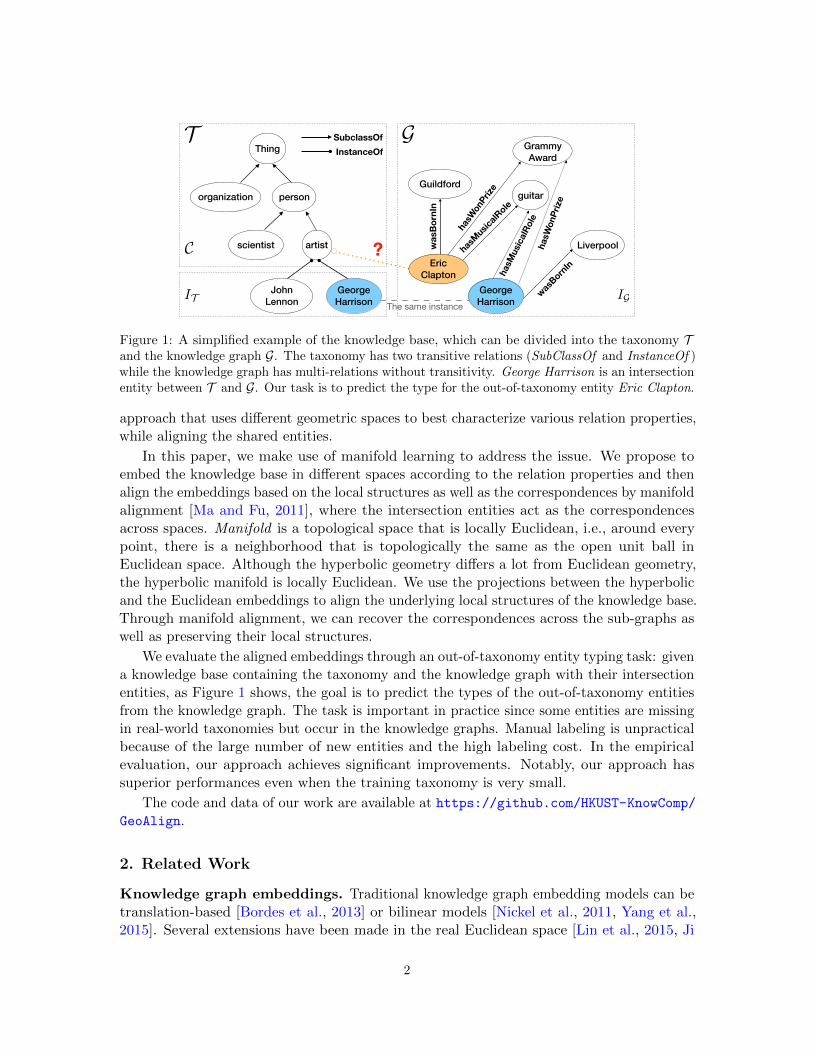
Figure 1: A simplified example of the knowledge base, which can be divided into the taxonomy Tand the knowledge graph G. The taxonomy has two transitive relations (SubClassOf and InstanceOf )while the knowledge graph has multi-relations without transitivity. George Harrison is an intersectionentity between T and G. Our task is to predict the type for the out-of-taxonomy entity Eric Clapton.

approach that uses different geometric spaces to best characterize various relation properties,while aligning the shared entities.

In this paper, we make use of manifold learning to address the issue. We propose toembed the knowledge base in different spaces according to the relation properties and thenalign the embeddings based on the local structures as well as the correspondences by manifoldalignment [Ma and Fu, 2011], where the intersection entities act as the correspondencesacross spaces. Manifold is a topological space that is locally Euclidean, i.e., around everypoint, there is a neighborhood that is topologically the same as the open unit ball inEuclidean space. Although the hyperbolic geometry differs a lot from Euclidean geometry,the hyperbolic manifold is locally Euclidean. We use the projections between the hyperbolicand the Euclidean embeddings to align the underlying local structures of the knowledge base.Through manifold alignment, we can recover the correspondences across the sub-graphs aswell as preserving their local structures.

We evaluate the aligned embeddings through an out-of-taxonomy entity typing task: givena knowledge base containing the taxonomy and the knowledge graph with their intersectionentities, as Figure 1 shows, the goal is to predict the types of the out-of-taxonomy entitiesfrom the knowledge graph. The task is important in practice since some entities are missingin real-world taxonomies but occur in the knowledge graphs. Manual labeling is unpracticalbecause of the large number of new entities and the high labeling cost. In the empiricalevaluation, our approach achieves significant improvements. Notably, our approach hassuperior performances even when the training taxonomy is very small.

The code and data of our work are available at https://github.com/HKUST-KnowComp/GeoAlign.

2. Related Work

Knowledge graph embeddings. Traditional knowledge graph embedding models can betranslation-based [Bordes et al., 2013] or bilinear models [Nickel et al., 2011, Yang et al.,2015]. Several extensions have been made in the real Euclidean space [Lin et al., 2015, Ji

2

https://github.com/HKUST-KnowComp/GeoAlign

https://github.com/HKUST-KnowComp/GeoAlign

Manifold Alignment across Geometric Spaces for Knowledge Base Representation Learning

et al., 2015, Sun et al., 2019] and the complex Euclidean space [Trouillon et al., 2016, Zhanget al., 2019]. It is shown that several properties of relations such as symmetry, inversion,and composition can be well handled by the Euclidean space [Sun et al., 2019].

Hierarchy-aware knowledge graph embeddings. Some works made special effortsfor transitive relations in the Euclidean space. TransC [Lv et al., 2018] encoded types asspheres and entities as vectors for modeling the hypernymy relation HAKE [Zhang et al.,2020] proposed to map entities into the Euclidean polar coordinate system. JOIE [Hao et al.,2019] separated the knowledge base into the taxonomy and the remaining knowledge graph,which had the same setting as our work. It then leveraged a non-linear transformationbetween two Euclidean embedding models. However, the non-linear affine transformation isnot powerful enough to build correlations between two underlying structures.

Hyperbolic embeddings. Hyperbolic embeddings have gained much attention in recentyears. [Nickel and Kiela, 2017] proposed to use the Poncare ball model of the hyperbolicspace to learn the graph embeddings. [Ganea et al., 2018, Nickel and Kiela, 2018, Becigneuland Ganea, 2019, Sala et al., 2018, Gu et al., 2019, Sonthalia and Gilbert, 2020] then furtherimproved hyperbolic embeddings. These methods perform well on data with hierarchicalstructures and single transitive relation, but they cannot predict the out-of-taxonomy entities,thus are not directly applicable to our entity typing task. Motivated by the above works,MurP [Balazevic et al., 2019], AttH [Chami et al., 2020], and HyperKA [Sun et al., 2020]explored the multi-relational knowledge graph embeddings in the hyperbolic space. However,most relations in knowledge graphs do not have transitivity, thus do not fit the hyperbolicspace. Their experimental results only significantly improved on transitive relations or thedatasets with natural hierarchical structures.

Manifold alignment. Manifold alignment [Ham et al., 2003, Ma and Fu, 2011] is a classof algorithms aligning the local structures and transferring knowledge across data sets. Inthis work, we use two-step alignment [Lafon et al., 2006, Wang and Mahadevan, 2008], whichutilizes the Laplacian eigenmaps [Belkin and Niyogi, 2003].

Note that our work focuses on a different research topic with the knowledge graph entityalignment [Hao et al., 2016, Sun et al., 2020] and the ontology matching [Alvarez-Melis et al.,2020] since entity alignment/matching aligns the entities that referring to the same thingbut having different names, while in our work, the correspondences between the knowledgegraph and the taxonomy are already known and we make use of the correspondences toapply manifold alignment and then predict the new out-of-taxonomy entities’ types.

3. Problem Formulation

Given a knowledge base B containing the taxonomy T and the knowledge graph G, we aim tolearn the alignment between the embeddings of T and G. An example of B is shown in Figure1. The taxonomy T contains the type set C = {Thing, organization, person, scientist, artist},the entity set IT = {John Lennon,George Harrison}, and the directed edge set ET = {ei,j :i, j ∈ C ∪ IT }, where ei,j represents that i and j have the transitive relation, e.g., (JohnLennon, InstanceOf, artist) and (artist, SubClassOf, person).

3

Denote the entity set and the relation set of the knowledge graph G as IG and RGrespectively,1 then G is composed of the triplets F = {(h, r, t) : h, t ∈ IG , r ∈ RG}, e.g., (EricClapton, wasBornIn, Guildford). There are some intersection entities between T and G,which we denote as Icor: Icor = IT ∩ IG . In Figure 1, Icor ={George Harrison}.

To apply manifold alignment, first, we need to obtain the pretrained embeddings of ITand IG , denoted as IT and IG . IT ∈ Hn, IG ∈ Rm, where Hn is the n-dimensional hyperbolicspace, and Rm is the m-dimensional Euclidean space. Then manifold alignment is appliedto project IT and IG into a shared manifold. After that, we have the embeddings of allentities of B in the same manifold. Note that here all entities do not include types in C inthe taxonomy. In the out-of-taxonomy entity typing task, the goal is to predict the types ofthe new entities from In = IG − IT . It can also be regarded as a taxonomy completion task.

4. Approach

The main framework of our approach involves three parts: pretraining, manifold alignment,and retraining the taxonomy with new entities. We give the details in the following.

4.1 Pretraining of Taxonomy and Knowledge Graph Embeddings

In our work, we use the hyperboloid model of hyperbolic embeddings [Nickel and Kiela,2018] to learn the taxonomy embeddings. The background of the hyperbolic space andthe hyperboloid model are in Appendix A. For the knowledge graph, we employ TransEproposed by [Bordes et al., 2013], which is a classical and effective embedding algorithm.

4.1.1 Hyperbolic Embeddings in the Hyperboloid Model

Given the taxonomy T with type set C, entity set IT , and edge set ET , the objective isto find the embeddings of the types and entities T = {Ti},Ti ∈ Hn, where Hn is then-dimensional hyperboloid model (Hn is one model of Hn). The soft ranking loss is

LT =∑

(xi,xj)∈ET

loge−dh(Ti,Tj)∑

xk∈N (xi)e−dh(Ti,Tk)

, (1)

where N (xi) = {xk : (xi, xk) /∈ ET } ∪ {xi} is the set of negative examples for xi togetherwith xi. The hyperboloid model Hn and its distance function dh are defined in Appendix A.

The minimization of LT makes the connected entities and types closer than those withno observed edges. Riemannian SGD (RSGD) [Bonnabel, 2013] is applied to train thehyperbolic embeddings.

4.1.2 TransE for Knowledge Graph Embeddings

Given a triplet (h, r, t), by regarding d(h + r, t) as the energy of (h, r, t), where h, r, t arethe corresponding embeddings and d is some dissimilarity measure (usually the L1 or L2

1. We suppose the knowledge graph G does not have transitive relations since all edges with transitiverelations are in the taxonomy.

4


norm), the margin-based ranking loss over the knowledge graph G with the triplet set F is

LG =∑

(h,r,t)∈F

∑(h′,r,t′)∈N (h,r,t)

[γ + d(h + r, t)− d(h′ + r, t′)]+, (2)

for some margin γ > 0. [x]+ = max(0, x) and N (h, r, t) = {(h′, r, t)|h′ ∈ IG} ∪ {(h, r, t′)|t′ ∈IG} is the negative sample set. The optimization of LG encourages positive triplets to satisfyh + r ≈ t and negative ones to satisfy that h + r is far away from t.

4.2 Manifold Alignment

After pretraining, we conduct manifold alignment to learn the aligned embeddings of thetaxonomy entities IT and knowledge graph entities IG in a shared manifold. The goalof manifold alignment is to find the projection functions such that the projections notonly minimize the distance between the corresponding points but also preserve the localmanifold structures of the original data. In our framework, given two entity sets IT , IG , andtheir embeddings IT ∈ Hn, IG ∈ Rm, we aim to learn the projections φIT : Hn → Rd andφIG : Rm → Rd. The algorithm works as follows:

First, we construct the binary correspondence matrix W using the intersection set Icor:

Wij =

{1 if (IT )i ↔ (IG)j ,0 otherwise.

(3)

Next, we construct the adjacency graphs from IT and IG . Specifically, we compute thepointwise distances within the two sets and select the k nearest neighbors (k-nn) to constructthe adjacency matrices AT and AG , i.e., ATij = 1 if and only if entity i (or j) is among the k

nearest neighbors of entity j (or i), and the same with AG . Then we construct the similaritymatrices ST and SG using heat kernel:

STij = exp(−dh(ITi , I

Tj )

t) ·ATij , SGij = exp(−

d(IGi , IGj )

t) ·AGij , (4)

where t > 0 is the parameter of heat kernel. dh refers to the hyperboloid distance inAppendix A, and d is the L2 norm in the Euclidean space. The manifold alignment loss isdefined as:

LM =µ

[∑i,j

‖φIT (ITi )− φIT (ITj )‖2STij +∑i,j

‖φIG (IGi )− φIG (IGj )‖2SGij]

+ (1− µ)∑i,j

‖φIT (ITi )− φIG (IGj )‖2Wij , (5)

where 0 ≤ µ ≤ 1 is the weight to balance between preserving the original manifold structuresand minimizing the corresponding entity distances. The first term multiplied by µ infer thatif two entities both from IT or both from IG are similar, their projections in the latent spaceshould be close with each other. If two entities from IT and IG are the same entity, the lastterm minimizes the distance between their projections in the shared manifold.

5

In practice, an additional constraint needs to be added in Eq. (5) to avoid the all-zerosolution. More details are given in Appendix B.1. Then minimizing LM is equivalent tosolving a generalized eigenvalue problem of the joint graph Laplacian L: Lv = λDv.

Denote the joint matrix J =

[µST (1− µ)W

(1− µ)W T µSG

], D is a diagonal matrix and

Dii =∑

j Jji =∑

j Jij (the proof of J ’s symmetry can be referred to Appendix B.2), thenthe Laplacian L = D − J is a symmetric and positive semidefinite matrix (see AppendixB.3 for proof). Let v0, . . . ,vd be the solutions ordered according to their eigenvalues, i.e.,Lvi = λiDvi for 0 ≤ i ≤ d, and 0 = λ0 ≤ λ1 ≤ · · · ≤ λd. Then the trivial eigenvector v0

is discarded and the next d eigenvectors are used for the aligned embeddings (proved inAppendix B.4). That means the embedding vectors for IT and IG in the shared manifold are

φIT (ITi ) = (v1(i), . . . ,vd(i)), 1 ≤ i ≤ |IT |, (6)

φIG (IGj ) = (v1(|IT |+ j), . . . ,vd(|IT |+ j)), 1 ≤ j ≤ |IG |. (7)

Following the above procedure, we project both entity sets into a shared manifold. Thealigned embeddings are learned by preserving the original manifold structure and recoveringthe correspondences. They provide correlations between IT and IG .

4.3 Linking New Entities and Retraining

Once we obtain the aligned embeddings φIT (IT ), φIG (IG) ∈ Rd, we can compute the pairwisedistances of the entities in the shared manifold. From the pairwise distances, we furtherconnect IT and In = IG − IT by k-nn and thus have the new edges En = {(xi, xj) : xi ∈IT , xj ∈ In}.

Next, we retrain the hyperbolic embeddings of the completed taxonomy with ET ∪ En.Note that En is different with ET since ET is the set of original taxonomy edges representingthe transitive relation among types and entities while edges in En reveal the similaritiesbetween entities. To differentiate them, we regard the edges in En as weighted undirectededges during training. That is to say, we append (xi, xj) and (xj , xi) to the training set if(xi, xj) ∈ En. Moreover, we let the terms associating with En in the loss (Eq. (1)) multiplyby a weight, which adjusts the weight of the newly-added undirected edges.

Again we use RSGD to update the hyperbolic embeddings. Then we can predict thelinks between the new entities In and the types C according to the hyperboloid distance.

5. Experiments

In this section, we evaluate the performance of our approach on the out-of-taxonomy entitytyping task. We report the main results here. For more experiments, please see Appendix D.

5.1 Experimental Settings

5.1.1 Data

We construct our knowledge bases from YAGO3 [Mahdisoltani et al., 2015], a huge semanticknowledge base derived from Wikipedia, WordNet, and GeoNames. Consistent with ourframework, YAGO3 is divided into the taxonomy and the knowledge graph. We provide the

6


Taxonomy KGYAGOwordnet wikiObjects YAGOfacts

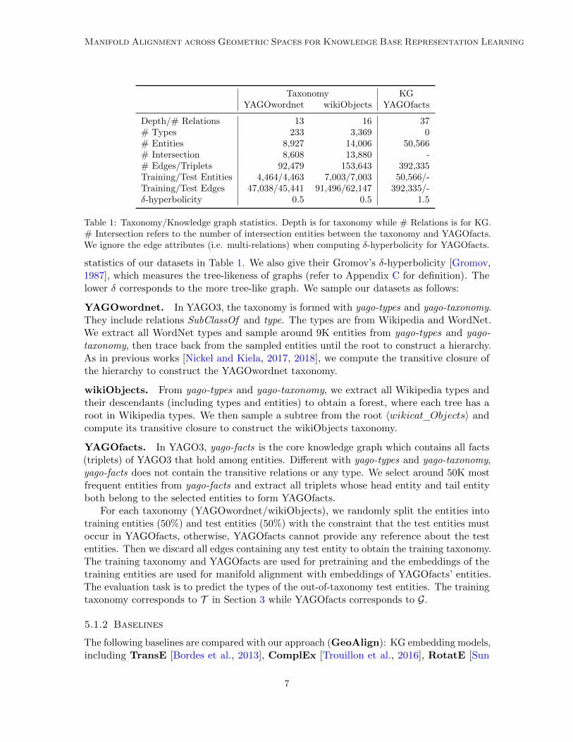
Depth/# Relations 13 16 37# Types 233 3,369 0# Entities 8,927 14,006 50,566# Intersection 8,608 13,880 -# Edges/Triplets 92,479 153,643 392,335Training/Test Entities 4,464/4,463 7,003/7,003 50,566/-Training/Test Edges 47,038/45,441 91,496/62,147 392,335/-δ-hyperbolicity 0.5 0.5 1.5

Table 1: Taxonomy/Knowledge graph statistics. Depth is for taxonomy while # Relations is for KG.# Intersection refers to the number of intersection entities between the taxonomy and YAGOfacts.We ignore the edge attributes (i.e. multi-relations) when computing δ-hyperbolicity for YAGOfacts.

statistics of our datasets in Table 1. We also give their Gromov’s δ-hyperbolicity [Gromov,1987], which measures the tree-likeness of graphs (refer to Appendix C for definition). Thelower δ corresponds to the more tree-like graph. We sample our datasets as follows:

YAGOwordnet. In YAGO3, the taxonomy is formed with yago-types and yago-taxonomy.They include relations SubClassOf and type. The types are from Wikipedia and WordNet.We extract all WordNet types and sample around 9K entities from yago-types and yago-taxonomy, then trace back from the sampled entities until the root to construct a hierarchy.As in previous works [Nickel and Kiela, 2017, 2018], we compute the transitive closure ofthe hierarchy to construct the YAGOwordnet taxonomy.

wikiObjects. From yago-types and yago-taxonomy, we extract all Wikipedia types andtheir descendants (including types and entities) to obtain a forest, where each tree has aroot in Wikipedia types. We then sample a subtree from the root 〈wikicat Objects〉 andcompute its transitive closure to construct the wikiObjects taxonomy.

YAGOfacts. In YAGO3, yago-facts is the core knowledge graph which contains all facts(triplets) of YAGO3 that hold among entities. Different with yago-types and yago-taxonomy,yago-facts does not contain the transitive relations or any type. We select around 50K mostfrequent entities from yago-facts and extract all triplets whose head entity and tail entityboth belong to the selected entities to form YAGOfacts.

For each taxonomy (YAGOwordnet/wikiObjects), we randomly split the entities intotraining entities (50%) and test entities (50%) with the constraint that the test entities mustoccur in YAGOfacts, otherwise, YAGOfacts cannot provide any reference about the testentities. Then we discard all edges containing any test entity to obtain the training taxonomy.The training taxonomy and YAGOfacts are used for pretraining and the embeddings of thetraining entities are used for manifold alignment with embeddings of YAGOfacts’ entities.The evaluation task is to predict the types of the out-of-taxonomy test entities. The trainingtaxonomy corresponds to T in Section 3 while YAGOfacts corresponds to G.

5.1.2 Baselines

The following baselines are compared with our approach (GeoAlign): KG embedding models,including TransE [Bordes et al., 2013], ComplEx [Trouillon et al., 2016], RotatE [Sun

7

et al., 2019]; hierarchy-aware Euclidean methods, including TransC [Lv et al., 2018],HAKE [Zhang et al., 2020], JOIE [Hao et al., 2019]; multi-relational hyperbolic models:MurP [Balazevic et al., 2019], AttH [Chami et al., 2020], HyperKA [Sun et al., 2020].

5.1.3 Training and Evaluation

To apply the baselines to our task, they are trained on all triplets of YAGOfacts combinedwith the training taxonomy, where the taxonomy edges are labeled as 〈isA〉. Then the testtriplets are {(xi, 〈isA〉, Cj)} where xi is a test entity and Cj is xi’s ground-truth type.

For knowledge graph embedding models, we use the OpenKE repository [Han et al.,2018] to train them while for other baselines, we use their public codes. For all methods, wetune the hyperparameters on the knowledge base combining YAGOwordnet and YAGOfactsby grid search according to MAP score. The hyperparameters are given in Appendix D.1.

We use the mean average precision (MAP), mean reciprocal rank (MRR), and theproportion of correct types that rank no larger than N (Hits@N) as our evaluation metrics,which are widely used for evaluating ranking and link prediction. The details of predictionsteps and the evaluation metrics are given in Appendix D.2. In our experiments, eachrunning is executed 5 times and the mean values of results are reported.

5.2 Overall Results

Table 2 presents the results in 50-dimensional embedding spaces. The results show thatGeoAlign has the best performance on wikiObjects while having a very close performancewith MurP on YAGOwordnet. In fact, wikiObjects is more challenging since its taxonomyis more massive (see Appendix D.3 for the case study), making it more difficult to find allcorrect types for the out-of-taxonomy entity.

From Table 2, we see that the traditional Euclidean models (TransE, ComplEx, andRotatE) are not capable of inferring the transitive relation, which is consistent with previousworks on hyperbolic embeddings [Nickel and Kiela, 2017, 2018]. The hierarchy-aware methods(TransC, HAKE, and JOIE) have better results than the traditional Euclidean embeddings,but overall they cannot achieve comparative performances with the hyperbolic models.

For the multi-relational hyperbolic models, MurP and AttH, which use different relationparameterizations on the base of Poincare embeddings, reveal their strengths. MurP, AttH,and GeoAlign all take advantage of the hyperbolic geometry for the taxonomy embeddings,thus having close results on the entity typing task. However, in Section 5.4, we will show thatGeoAlign has significant improvements over MurP and AttH when the training taxonomy isvery small. Furthermore, MurP and AttH can only do the inference for all relation propertiesin the hyperbolic space, which is not suitable for the non-transitive relation properties,while GeoAlign can take advantage of any base embedding models rather than TransE forpretraining the knowledge graph. As for HyperKA, which leverages hyperbolic GNN forembeddings, we tried our best to tune the model, but it still cannot achieve promisingresults. We think the neural models may not fit this task setting and our datasets. Thatalso accounts for why AttH is not as good as MurP. Compared with MurP, AttH adds theattention mechanism and has more complicated parameterizations. It may hurt the model’sfeasibility sometimes.

8


YAGOwordnet wikiObjectsMAP MRR Hits@1 Hits@3 MAP MRR Hits@1 Hits@3

TransE ‡21.36 ‡6.91 ‡19.67 ‡27.95 ‡13.68 ‡6.51 ‡14.52 ‡24.10ComplEx ‡50.77 ‡13.63 ‡20.09 ‡48.82 ‡28.10 ‡15.13 ‡24.30 ‡33.89RotatE ‡70.72 ‡21.63 ‡64.63 ‡88.28 ‡62.42 ‡32.38 ‡66.85 ‡81.78

TransC ‡84.25 ‡26.35 ‡93.72 †99.29 ‡67.87 ‡34.24 ‡81.87 ‡93.26HAKE ‡74.52 ‡18.77 ‡51.22 ‡58.86 †66.50 †30.53 ‡52.93 ‡61.02JOIE 94.92 28.15 ‡97.20 99.60 ‡86.67 ‡41.87 ‡93.00 ‡98.94

MurP †94.41 28.20 99.57 †99.84 ‡88.48 ‡42.77 ‡99.80 100.00AttH 94.80 28.19 ‡97.76 99.88 88.40 ‡42.65 ‡98.34 †99.90HyperKA ‡55.83 ‡19.15 ‡64.84 ‡83.84 ‡48.02 ‡27.42 ‡59.80 ‡74.73

GeoAlign ‡94.04 28.19 †99.13 99.92 88.67 42.82 99.89 100.00

Table 2: Results of MAP(%), MRR(%), and Hits@N(%) in 50-dimensional embedding spaces. Thebest results are shown in boldface and the second-best results are underlined. The statisticallysignificance metrics are marked with either † if p-values < 0.05 or ‡ if p-values < 0.001.

Dimension 5 10 20 100MRR Hits@1 MRR Hits@1 MRR Hits@1 MRR Hits@1

TransE ‡2.42 ‡3.91 ‡5.41 ‡9.91 ‡6.80 ‡14.14 ‡8.77 ‡19.21ComplEx ‡0.09 ‡0.00 ‡11.97 ‡22.59 ‡14.32 ‡24.20 ‡20.21 ‡34.39RotatE ‡1.76 ‡1.39 ‡3.50 ‡2.94 ‡4.23 ‡3.37 ‡37.68 ‡79.95

TransC ‡32.62 ‡66.69 ‡36.15 ‡78.55 ‡36.67 ‡84.03 ‡34.28 ‡81.32HAKE ‡7.85 ‡12.62 ‡15.58 ‡22.70 ‡10.16 ‡17.29 †37.90 ‡70.88JOIE ‡27.76 ‡48.01 ‡39.93 ‡84.68 ‡41.64 ‡92.62 ‡42.12 ‡94.61

MurP ‡42.18 ‡98.19 ‡42.61 ‡98.59 ‡42.72 ‡99.60 42.91 ‡99.90AttH - - †40.60 †92.47 ‡42.10 ‡97.05 ‡42.78 ‡98.76HyperKA ‡16.93 ‡34.51 ‡21.65 ‡41.30 ‡19.00 ‡42.98 ‡24.51 ‡61.92

GeoAlign 42.74 99.64 42.83 99.84 42.81 99.92 ‡42.82 99.93

Table 3: Results of MRR(%) and Hits@1(%) in different embedding dimensions on wikiObjects. AttHrequires the dimension to be even because of the diagonal Givens transformations in its model, thusnot applicable to 5-dimensional space. The best results are shown in boldface and the second-bestresults are underlined. The statistically significance metrics are marked with either † if p-values< 0.05 or ‡ if p-values < 0.001.

5.3 Exploring the Embedding Dimensions

In this section, we explore the performances in different embedding dimensions. The resultsare presented in Table 3. For GeoAlign, JOIE, and HyperKA, the embedding dimensionsfor the knowledge graph and the taxonomy are both set as n for n ∈ {5, 10, 20, 100}. FromTable 3, we see that with the increase of the embedding dimension, most methods get betterresults. The Euclidean models can have big improvements in higher dimensions, such asRotatE from 20-d to 100-d, but their 100-d performances cannot surpass GeoAlign in 5-d.We also notice that some methods suffer from overfitting in high dimensions, e.g., TransC,HAKE, and HyperKA drop down when the dimension increases. In contrast, GeoAlign,MurP, and AttH achieve great results steadily. On the one hand, the hyperbolic modelsrequire much lower dimensions. On the other hand, 5-dimensional embeddings are already

9

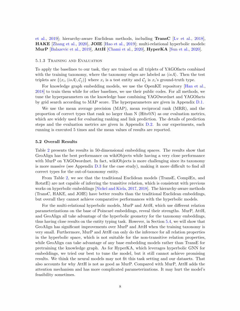
Training rate 0.1 0.2 0.3 0.4Training/Test entities 1,401/12,605 2,802/11,204 4,202/9,804 5,603/8,403Training/Test edges 42,764/110,879 54,637/99,006 67,788/85,855 80,190/73,453

MurP ‡82.83 ‡86.56 ‡88.16 ‡88.45AttH †84.32 ‡86.62 ‡87.80 88.40GeoAlign 88.50 88.78 89.09 88.90

Table 4: Results of MAP(%) under different training rates on wikiObjects in 50-dimension. Thetraining rate is used to randomly split the taxonomy entities. Training edges represents the number oftraining edges in the training taxonomy wikiObjects (the training edges of YAGOfacts is 392,335 allthe time). The best results are shown in boldface. The statistically significance metrics are markedwith either † if p-values < 0.05 or ‡ if p-values < 0.001.

enough for GeoAlign to learn the manifold alignment between the local structures of theknowledge base.

5.4 Results on Small Training Rates

In Section 5.2, we see that the performances of MurP, AttH, and GeoAlign are very closeunder the training rate=0.5. Here we explore their performances on smaller training rates.For the training rate r ∈ {0.1, 0.2, 0.3, 0.4}, we randomly split the entities into trainingentities (r) and test entities (1 − r). The splitting and training taxonomy constructionprocedure are the same as described in Section 5.1.1. Note that the small training ratemeans that the pretrained taxonomy and the number of taxonomy entities used for manifoldalignment are both small. We report the MAP(%) scores in Table 4. We find that whenthe training rate is small, GeoAlign outperforms MurP and AttH significantly. With theincrease of the training rates, their performances get more and more similar and converge tostable. The results demonstrate the effectiveness of our approach on small training rates.

5.5 Ablation Study

5.5.1 On the Retraining Step

To analyze the benefits and the potential defects of the retraining step after manifoldalignment, we compare the performances of GeoAlign with and without retraining on twotasks. The first task is the out-of-taxonomy entity typing task, which is the same as the aboveexperiments. The -w/o retraining method works in the way that after manifold alignment,we directly predict the types of the test entities as the types of its nearest neighbor accordingto the aligned embeddings. If its nearest neighbor is not in the taxonomy’s training entities,we find the next nearest one until it does. The second task is graph reconstruction ofthe training taxonomy. We intend to see whether the retrained model with new entitiescompromises the representation of the original taxonomy. We report the results in Table 5.

The entity typing results demonstrate that after manifold alignment, the retrainingof the embeddings with the added edges incorporates more structural information of thetaxonomy with new entities and improves the performances significantly. The reconstructionresults show that the retraining has little impact on the original training taxonomy. Thecompromise is acceptable, especially when considering the remarkable improvements on theentity typing task (more than 10% MAP improvements in Table 5).

10


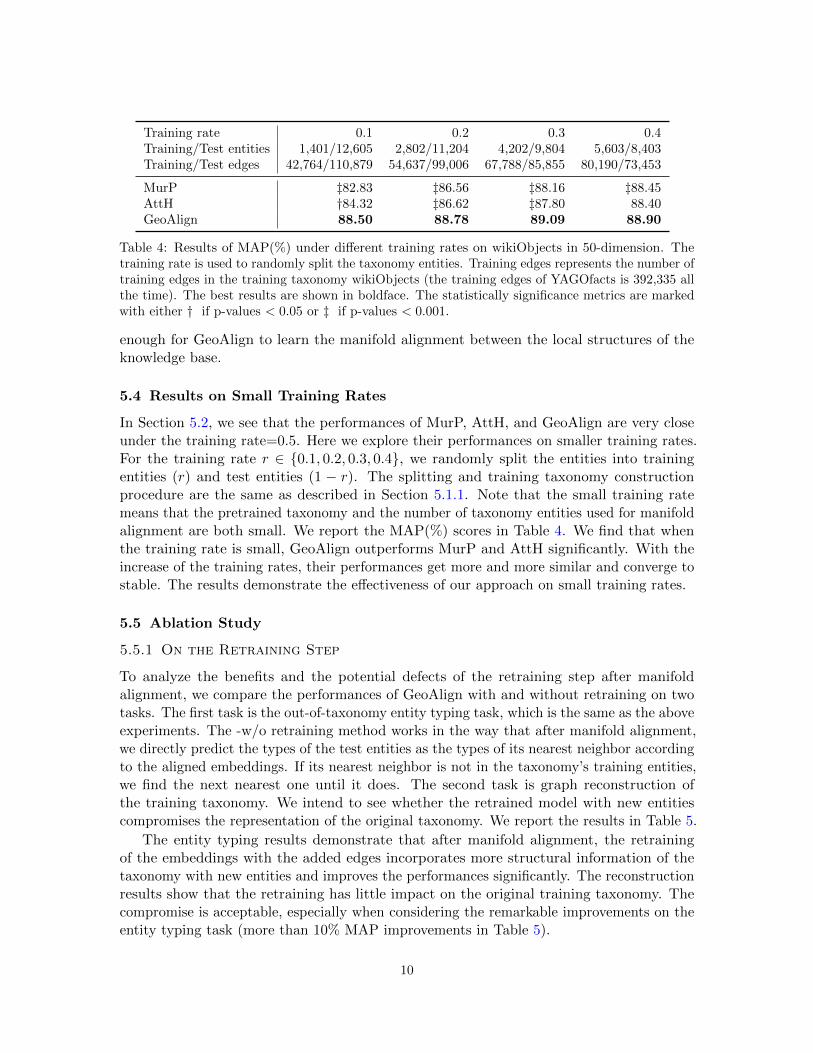
YAGOwordnet wikiObjectsMAP MRR MAP MRR

Entity typingGeoAlign 94.04 28.19 88.67 42.82-w/o retraining 84.98 - 71.75 -

ReconstructionGeoAlign 95.40 28.70 89.69 39.17-w/o retraining 97.06 29.02 90.99 39.56

Table 5: Ablation study for GeoAlign in 50-dimension. Entity typing is the out-of-taxonomy entitytyping task and Reconstruction is the training taxonomy reconstruction task. Since -w/o retrainingdoes not obtain a rank for all types on entity typing task, MRR is not applicable.

MAP MRR

Entity typingGeoAlign-hyperboloid 94.04 28.19GeoAlign-Poincare 84.30 26.56

ReconstructionGeoAlign-hyperboloid 95.40 28.70GeoAlign-Poincare 91.68 28.11

Table 6: Ablation study of the hyperbolic models on YAGOwordnet in 50-dimension. Entity typingis the out-of-taxonomy entity typing and Reconstruction is the training taxonomy reconstruction.

5.5.2 On the Hyperbolic Models

To compare the different hyperbolic models, we evaluate the performances of GeoAlign withthe hyperboloid model and the Poincare ball model on two tasks. Again, the first task isthe out-of-taxonomy entity typing task and the second task is graph reconstruction of thetraining taxonomy. The MAP(%) and MRR(%) scores are reported in Table 6. GeoAlign-hyperboloid (Poincare) means we pretrain and retrain the taxonomy by the hyperboloidembeddings (Poincare ball embeddings). From Table 6, we see that GeoAlign-hyperboloidsurpasses GeoAlign-Poincare a lot, especially on the out-of-taxonomy entity typing task.

6. Conclusion and Future Work

We propose to learn the embeddings of knowledge bases in different spaces and apply manifoldalignment across the geometric spaces to build the projection. The main motivation is toallow different geometric spaces to model the various properties of relations as well as thevarious local structures of the knowledge base, while manifold alignment provides a way toincorporate the local manifold structure of two entity sets. We propose a solid frameworkand evaluate our approach on an out-of-taxonomy entity typing task. The empirical resultsdemonstrate the superiority of our approach, especially in low dimensions and on smalltraining rates. Future works include the exploration of broader types of geometries forlearning embeddings and more effective approaches for aligning multiple manifolds.

Acknowledgment

The authors of this paper were supported by the NSFC Fund (U20B2053) from the NSFCof China, the RIF (R6020-19 and R6021-20) and the GRF (16211520) from RGC of HongKong, the MHKJFS (MHP/001/19) from ITC of Hong Kong.

11

References

David Alvarez-Melis, Youssef Mroueh, and Tommi S. Jaakkola. Unsupervised hierarchymatching with optimal transport over hyperbolic spaces. In AISTATS, volume 108, pages1606–1617, 2020.

Ivana Balazevic, Carl Allen, and Timothy M. Hospedales. Multi-relational poincare graphembeddings. In NeurIPS, pages 4465–4475, 2019.

Gary Becigneul and Octavian-Eugen Ganea. Riemannian adaptive optimization methods.In ICLR (Poster). OpenReview.net, 2019.

Mikhail Belkin and Partha Niyogi. Laplacian eigenmaps for dimensionality reduction anddata representation. Neural Computation, 15(6):1373–1396, 2003.

Silvere Bonnabel. Stochastic gradient descent on riemannian manifolds. IEEE Trans.Automat. Contr., 58(9):2217–2229, 2013.

Antoine Bordes, Nicolas Usunier, Alberto Garcıa-Duran, Jason Weston, and OksanaYakhnenko. Translating embeddings for modeling multi-relational data. In NIPS, pages2787–2795, 2013.

James W Cannon, William J Floyd, Richard Kenyon, Walter R Parry, et al. Hyperbolicgeometry. Flavors of geometry, 31:59–115, 1997.

Ines Chami, Adva Wolf, Da-Cheng Juan, Frederic Sala, Sujith Ravi, and Christopher Re.Low-dimensional hyperbolic knowledge graph embeddings. In ACL, pages 6901–6914.ACL, 2020.

Octavian-Eugen Ganea, Gary Becigneul, and Thomas Hofmann. Hyperbolic entailmentcones for learning hierarchical embeddings. In ICML, volume 80, pages 1632–1641, 2018.

Mikhael Gromov. Hyperbolic groups. In Essays in group theory, pages 75–263. Springer,1987.

Albert Gu, Frederic Sala, Beliz Gunel, and Christopher Re. Learning mixed-curvaturerepresentations in product spaces. In ICLR (Poster). OpenReview.net, 2019.

Ji Hun Ham, Daniel D Lee, and Lawrence K Saul. Learning high dimensional correspondencesfrom low dimensional manifolds. 2003.

Xu Han, Shulin Cao, Xin Lv, Yankai Lin, Zhiyuan Liu, Maosong Sun, and Juanzi Li. Openke:An open toolkit for knowledge embedding. In EMNLP (Demonstration), pages 139–144.ACL, 2018.

Junheng Hao, Muhao Chen, Wenchao Yu, Yizhou Sun, and Wei Wang. Universal representa-tion learning of knowledge bases by jointly embedding instances and ontological concepts.In KDD, pages 1709–1719. ACM, 2019.

12


Yanchao Hao, Yuanzhe Zhang, Shizhu He, Kang Liu, and Jun Zhao. A joint embeddingmethod for entity alignment of knowledge bases. In CCKS, volume 650, pages 3–14.Springer, 2016.

Guoliang Ji, Shizhu He, Liheng Xu, Kang Liu, and Jun Zhao. Knowledge graph embeddingvia dynamic mapping matrix. In ACL (1), pages 687–696. ACL, 2015.

Prodromos Kolyvakis, Alexandros Kalousis, and Dimitris Kiritsis. Hyperkg: Hyperbolicknowledge graph embeddings for knowledge base completion. CoRR, abs/1908.04895,2019.

Dmitri Krioukov, Fragkiskos Papadopoulos, Maksim Kitsak, Amin Vahdat, and MarianBoguna. Hyperbolic geometry of complex networks. Phys. Rev. E, 82:036106, Sep2010. doi: 10.1103/PhysRevE.82.036106. URL https://link.aps.org/doi/10.1103/

PhysRevE.82.036106.

Stephane Lafon, Yosi Keller, and Ronald R. Coifman. Data fusion and multicue datamatching by diffusion maps. TPAMI, 28(11):1784–1797, 2006.

Yankai Lin, Zhiyuan Liu, Maosong Sun, Yang Liu, and Xuan Zhu. Learning entity andrelation embeddings for knowledge graph completion. In AAAI, pages 2181–2187, 2015.

Nathan Linial, Eran London, and Yuri Rabinovich. The geometry of graphs and some of itsalgorithmic applications. Combinatorica, 15(2):215–245, 1995.

Xin Lv, Lei Hou, Juanzi Li, and Zhiyuan Liu. Differentiating concepts and instances forknowledge graph embedding. In EMNLP, pages 1971–1979. ACL, 2018.

Yunqian Ma and Yun Fu. Manifold learning theory and applications. CRC press, 2011.

Farzaneh Mahdisoltani, Joanna Biega, and Fabian M. Suchanek. YAGO3: A knowledgebase from multilingual wikipedias. In CIDR. www.cidrdb.org, 2015.

George A. Miller. Wordnet: A lexical database for english. Commun. ACM, 38(11):39–41,1995.

Maximilian Nickel and Douwe Kiela. Poincare embeddings for learning hierarchical represen-tations. In NIPS, pages 6338–6347, 2017.

Maximilian Nickel and Douwe Kiela. Learning continuous hierarchies in the lorentz modelof hyperbolic geometry. In ICML, volume 80, pages 3776–3785, 2018.

Maximilian Nickel, Volker Tresp, and Hans-Peter Kriegel. A three-way model for collectivelearning on multi-relational data. In ICML, pages 809–816, 2011.

Maximilian Nickel, Kevin Murphy, Volker Tresp, and Evgeniy Gabrilovich. A review ofrelational machine learning for knowledge graphs. Proceedings of the IEEE, 104(1):11–33,2016.

Frederic Sala, Christopher De Sa, Albert Gu, and Christopher Re. Representation tradeoffsfor hyperbolic embeddings. In ICML, volume 80, pages 4457–4466, 2018.

13

https://link.aps.org/doi/10.1103/PhysRevE.82.036106

https://link.aps.org/doi/10.1103/PhysRevE.82.036106

Rishi Sonthalia and Anna C. Gilbert. Tree! I am no tree! I am a low dimensional hyperbolicembedding. In NeurIPS, 2020.

Fabian M. Suchanek, Gjergji Kasneci, and Gerhard Weikum. Yago: a core of semanticknowledge. In WWW, pages 697–706. ACM, 2007.

Zequn Sun, Muhao Chen, Wei Hu, Chengming Wang, Jian Dai, and Wei Zhang. Knowledgeassociation with hyperbolic knowledge graph embeddings. In EMNLP (1), pages 5704–5716.ACL, 2020.

Zhiqing Sun, Zhi-Hong Deng, Jian-Yun Nie, and Jian Tang. Rotate: Knowledge graphembedding by relational rotation in complex space. In ICLR (Poster). OpenReview.net,2019.

Theo Trouillon, Johannes Welbl, Sebastian Riedel, Eric Gaussier, and Guillaume Bouchard.Complex embeddings for simple link prediction. In ICML, volume 48 of JMLR, pages2071–2080. JMLR.org, 2016.

Chang Wang and Sridhar Mahadevan. Manifold alignment using procrustes analysis. InICML, volume 307, pages 1120–1127, 2008.

Bishan Yang, Wen-tau Yih, Xiaodong He, Jianfeng Gao, and Li Deng. Embedding entitiesand relations for learning and inference in knowledge bases. In ICLR, 2015.

Shuai Zhang, Yi Tay, Lina Yao, and Qi Liu. Quaternion knowledge graph embeddings. InNeurIPS, pages 2731–2741, 2019.

Zhanqiu Zhang, Jianyu Cai, Yongdong Zhang, and Jie Wang. Learning hierarchy-awareknowledge graph embeddings for link prediction. In AAAI, 2020.

14


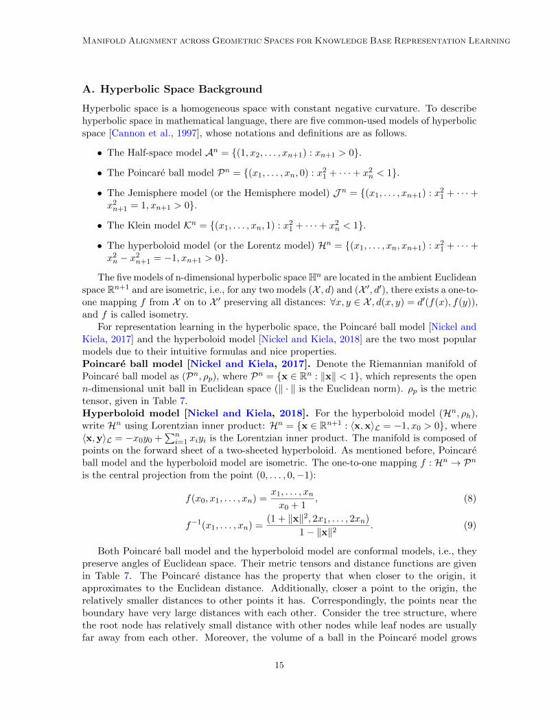
A. Hyperbolic Space Background

Hyperbolic space is a homogeneous space with constant negative curvature. To describehyperbolic space in mathematical language, there are five common-used models of hyperbolicspace [Cannon et al., 1997], whose notations and definitions are as follows.

• The Half-space model An = {(1, x2, . . . , xn+1) : xn+1 > 0}.

• The Poincare ball model Pn = {(x1, . . . , xn, 0) : x21 + · · ·+ x2

n < 1}.

• The Jemisphere model (or the Hemisphere model) J n = {(x1, . . . , xn+1) : x21 + · · ·+

x2n+1 = 1, xn+1 > 0}.

• The Klein model Kn = {(x1, . . . , xn, 1) : x21 + · · ·+ x2

n < 1}.

• The hyperboloid model (or the Lorentz model) Hn = {(x1, . . . , xn, xn+1) : x21 + · · ·+

x2n − x2

n+1 = −1, xn+1 > 0}.

The five models of n-dimensional hyperbolic space Hn are located in the ambient Euclideanspace Rn+1 and are isometric, i.e., for any two models (X , d) and (X ′, d′), there exists a one-to-one mapping f from X on to X ′ preserving all distances: ∀x, y ∈ X , d(x, y) = d′(f(x), f(y)),and f is called isometry.

For representation learning in the hyperbolic space, the Poincare ball model [Nickel andKiela, 2017] and the hyperboloid model [Nickel and Kiela, 2018] are the two most popularmodels due to their intuitive formulas and nice properties.Poincare ball model [Nickel and Kiela, 2017]. Denote the Riemannian manifold ofPoincare ball model as (Pn, ρp), where Pn = {x ∈ Rn : ‖x‖ < 1}, which represents the openn-dimensional unit ball in Euclidean space (‖ · ‖ is the Euclidean norm). ρp is the metrictensor, given in Table 7.Hyperboloid model [Nickel and Kiela, 2018]. For the hyperboloid model (Hn, ρh),write Hn using Lorentzian inner product: Hn = {x ∈ Rn+1 : 〈x,x〉L = −1, x0 > 0}, where〈x,y〉L = −x0y0 +

∑ni=1 xiyi is the Lorentzian inner product. The manifold is composed of

points on the forward sheet of a two-sheeted hyperboloid. As mentioned before, Poincareball model and the hyperboloid model are isometric. The one-to-one mapping f : Hn → Pnis the central projection from the point (0, . . . , 0,−1):

f(x0, x1, . . . , xn) =x1, . . . , xnx0 + 1

, (8)

f−1(x1, . . . , xn) =(1 + ‖x‖2, 2x1, . . . , 2xn)

1− ‖x‖2 . (9)

Both Poincare ball model and the hyperboloid model are conformal models, i.e., theypreserve angles of Euclidean space. Their metric tensors and distance functions are givenin Table 7. The Poincare distance has the property that when closer to the origin, itapproximates to the Euclidean distance. Additionally, closer a point to the origin, therelatively smaller distances to other points it has. Correspondingly, the points near theboundary have very large distances with each other. Consider the tree structure, wherethe root node has relatively small distance with other nodes while leaf nodes are usuallyfar away from each other. Moreover, the volume of a ball in the Poincare model grows

15

Model Metric tensor Distance function

Poincare ρp(x) = ( 21−‖x‖2 )2ρE(x) dp(x,y) = arcosh

(1 + 2 ‖x−y‖2

(1−‖x‖2)(1−‖y‖2)

)

Hyperboloid ρh(x) =

−1

1. . .

1

dh(x,y) = arcosh(−〈x,y〉L)

Table 7: Metric tensors and distance functions of Poincare ball model and the hyperboloid model.ρE(x) is the Euclidean metric. 〈x,y〉L is the Lorentzian inner product, 〈x,y〉L = −x0y0 +

∑ni=1 xiyi.

exponentially with its radius, resembling the tree-like property that the number of nodesgrows exponentially with depth in a tree. [Krioukov et al., 2010] built the approximateequivalence between hierarchical networks and the hyperbolic space. Nevertheless, whenusing the Poincare ball model for hierarchical structures [Nickel and Kiela, 2017], numericalinstabilities arise, which motivates the use of the hyperboloid model [Nickel and Kiela, 2018],since it can avoid the numerical instabilities from the fraction in distance function, henceallows for more efficient computation on the manifold. We provide the empirical evaluationof the two hyperbolic models in Section 5.5.2.

B. Proofs of Section 4.2 about Manifold Alignment

B.1 The Loss Function of Manifold Alignment

As presented in Section 4.2, the loss function includes two parts, one for preserving the localmanifold within each dataset, another for recovering the correspondence information.

We can rewrite LM using the joint adjacency matrix:

LM =∑i,j

‖Φi − Φj‖2Jij , (10)

where Φ is the unified representation of the taxonomy entities and the knowledge graph

entities, Φ =

[φIT (IT )φIG (IG)

]. J is the joint adjacency matrix, J =

[µST (1− µ)W

(1− µ)W T µSG

].

Eq. (10) is the loss function for Laplacian eigenmaps [Belkin and Niyogi, 2003], whichcan be further derived into:

LM =∑i,j

∑k

(Φi,k − Φj,k)2Jij =

∑k

∑i,j

(Φi,k − Φj,k)2Jij =

∑k

tr(ΦT·,kLΦ·,k) = tr(ΦTLΦ),

(11)where the Laplacian L = D − J and D is a diagonal matrix with Dii =

∑j Jji.

It is easily seen that mapping all entities to zero (Φ = 0) minimizes the loss function LM ,so an additional constraint ΦTDΦ = I needs to be added, where I is the identity matrix.

Theorem 1. Minimizing LM with the constraint ΦTDΦ = I to get the d-dimensional alignedembeddings (a (|IT |+ |IG |)× d matrix Φ) is equivalent to solving a generalized eigenvalueproblem of the joint graph Laplacian: Lv = λDv.

16


Proof. When d = 1, Φ is a (|IT |+ |IG |)-vector, denoted as v1, then we have

arg minv1:vT

1 Dv1=1LM = arg min

v1,λ:λ>0vT1 Lv1 + λ(1− vT1 Dv1). (12)

Differentiating Eq. (12) with respect to v1 and λ, we have

Lv1 = λDv1, (13)

vT1 Dv1 = 1. (14)

So the optimal v1 is a solution of the generalized eigenvalue problem: Lv1 = λDv1.Multiplying both sides of Eq. (13) by vT1 and applying Eq. (14), we have vT1 Lv1 = λ.To minimize LM = vT1 Lv1, we need to get the smallest nonzero eigenvalue λ1, then itscorresponding eigenvector v1 is the optimal solution.

When d > 1, Φ can be written as Φ = [v1,v2, . . . ,vd]. The optimization problem is

arg minΦ:ΦTDΦ=I

LM = arg minv1,...,vd,λ1,...,λd:λi>0

∑i

vTi Lvi + λi(1− vTi Dvi). (15)

Applying the same technique above, we have the minimal LM =∑

i λi, where λi, for i =1, . . . , d, are the d smallest nonzero eigenvalues sorted in ascending order: 0 < λ1 ≤ · · · ≤ λd,while their corresponding eigenvectors v1, . . . ,vd are the optimal solutions.

B.2 The Symmetry of J

Theorem 2. The joint adjacency matrix J =

[µST (1− µ)W

(1− µ)W T µSG

]is symmetric.

Proof. Recall the construction of the adjacency matrices AT and AG . ATij = 1 if and only ifentity i is among the k nearest neighbors of entity j or j is among the k nearest neighborsof i according to IT , and the same with AG . Thus AT and AG are symmetric.

Then the similarity matrices are constructed through Eq. (4). We have STij =

exp(−dh(ITi ,ITj )

t ) · ATij = exp(−dh(ITi ,ITj )

t ) · ATji = STji , similarly SGij = SGji, so ST and SG

are symmetric. Then J is also symmetric.

B.3 The Symmetry and Positive Semi-Definiteness of L

Theorem 3. The Laplacian L = D − J is symmetric and positive semidefinite.

Proof. First, L is symmetric because D and J are both symmetric (D is a diagonal matrixand J is proved in Appendix B.2).

Next, from Eqs. (10) and (11), we have∑

i,j ‖Φi − Φj‖2Ji,j = tr(ΦTLΦ), which showsthat L is positive semi-definite.

B.4 The Solutions of Manifold Alignment

Theorem 4. The generalized eigenvalue problem Lv = λDv has a zero eigenvalue λ0 = 0.

17

Proof. Since L = D − J , Dii =∑

j Jji =∑

j Jij ,

then (L · [1, 1, . . . , 1]T )i =∑

j Lij = Dii −∑

j(Jij) = 0,

that is, L · [1, 1, . . . , 1]T = 0, so λ0 = 0.

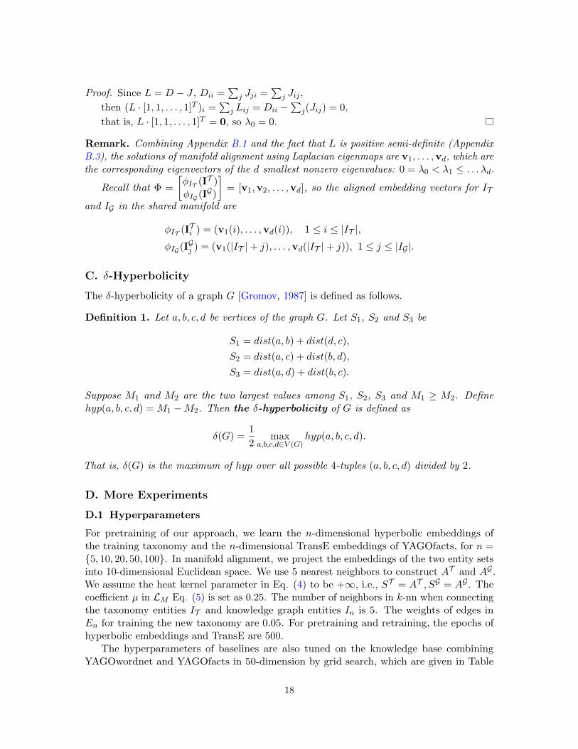
Remark. Combining Appendix B.1 and the fact that L is positive semi-definite (AppendixB.3), the solutions of manifold alignment using Laplacian eigenmaps are v1, . . . ,vd, which arethe corresponding eigenvectors of the d smallest nonzero eigenvalues: 0 = λ0 < λ1 ≤ . . . λd.

Recall that Φ =

[φIT (IT )φIG (IG)

]= [v1,v2, . . . ,vd], so the aligned embedding vectors for IT

and IG in the shared manifold are

φIT (ITi ) = (v1(i), . . . ,vd(i)), 1 ≤ i ≤ |IT |,φIG (IGj ) = (v1(|IT |+ j), . . . ,vd(|IT |+ j)), 1 ≤ j ≤ |IG |.

C. δ-Hyperbolicity

The δ-hyperbolicity of a graph G [Gromov, 1987] is defined as follows.

Definition 1. Let a, b, c, d be vertices of the graph G. Let S1, S2 and S3 be

S1 = dist(a, b) + dist(d, c),

S2 = dist(a, c) + dist(b, d),

S3 = dist(a, d) + dist(b, c).

Suppose M1 and M2 are the two largest values among S1, S2, S3 and M1 ≥ M2. Definehyp(a, b, c, d) = M1 −M2. Then the δ-hyperbolicity of G is defined as

δ(G) =1

2max

a,b,c,d∈V (G)hyp(a, b, c, d).

That is, δ(G) is the maximum of hyp over all possible 4-tuples (a, b, c, d) divided by 2.

D. More Experiments

D.1 Hyperparameters

For pretraining of our approach, we learn the n-dimensional hyperbolic embeddings ofthe training taxonomy and the n-dimensional TransE embeddings of YAGOfacts, for n ={5, 10, 20, 50, 100}. In manifold alignment, we project the embeddings of the two entity setsinto 10-dimensional Euclidean space. We use 5 nearest neighbors to construct AT and AG .We assume the heat kernel parameter in Eq. (4) to be +∞, i.e., ST = AT , SG = AG . Thecoefficient µ in LM Eq. (5) is set as 0.25. The number of neighbors in k-nn when connectingthe taxonomy entities IT and knowledge graph entities In is 5. The weights of edges inEn for training the new taxonomy are 0.05. For pretraining and retraining, the epochs ofhyperbolic embeddings and TransE are 500.

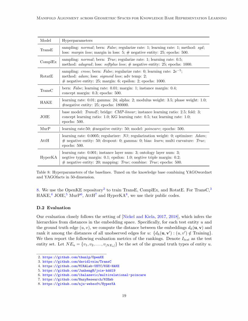
The hyperparameters of baselines are also tuned on the knowledge base combiningYAGOwordnet and YAGOfacts in 50-dimension by grid search, which are given in Table

18


Model Hyperparameters

TransEsampling: normal ; bern: False; regularize rate: 1; learning rate: 1; method: sgd ;loss: margin loss; margin in loss: 5; # negative entity: 25; epochs: 500.

ComplExsampling: normal ; bern: True; regularize rate: 1; learning rate: 0.5;method: adagrad ; loss: softplus loss; # negative entity: 25; epochs: 1000.

RotatEsampling: cross; bern: False; regularize rate: 0; learning rate: 2e−5;method: adam; loss: sigmoid loss; adv temp: 2;# negative entity: 25; margin: 6; epsilon: 2; epochs: 1000.

TransCbern: False; learning rate: 0.01; margin: 1; instance margin: 0.4;concept margin: 0.3; epochs: 500.

HAKElearning rate: 0.01; gamma: 24; alpha: 2; modulus weight: 3.5; phase weight: 1.0;#negative entity: 25; epochs: 180000.

JOIEbase model: TransE ; bridge: CMP-linear ; instance learning ratio: 2.5; fold: 3;concept learning ratio: 1.0; KG learning rate: 0.5; tax learning rate: 1.0;epochs: 500.

MurP learning rate:50; #negative entity: 50; model: poincare; epochs: 500.

AttHlearning rate: 0.0005; regularizer: N3 ; regularization weight: 0; optimizer: Adam;# negative entity: 50; dropout: 0; gamma: 0; bias: learn; multi curvature: True;epochs: 500.

HyperKAlearning rate: 0.001; instance layer num: 3; ontology layer num: 3;negtive typing margin: 0.1; epsilon: 1.0; negtive triple margin: 0.2;# negative entity: 20; mapping: True; combine: True; epochs: 500.

Table 8: Hyperparameters of the baselines. Tuned on the knowledge base combining YAGOwordnetand YAGOfacts in 50-dimension.

8. We use the OpenKE repository2 to train TransE, ComplEx, and RotatE. For TransC,3

HAKE,4 JOIE,5 MurP6, AttH7 and HyperKA8, we use their public codes.

D.2 Evaluation

Our evaluation closely follows the setting of [Nickel and Kiela, 2017, 2018], which infers thehierarchies from distances in the embedding space. Specifically, for each test entity u andthe ground truth edge (u, v), we compute the distance between the embeddings dh(u,v) andrank it among the distances of all unobserved edges for u: {dh(u,v′) : (u, v′) /∈ Training}.We then report the following evaluation metrics of the rankings. Denote Itest as the testentity set. Let NEu = {v1, v2, . . . , v|NEu|} be the set of the ground truth types of entity u.

2. https://github.com/thunlp/OpenKE3. https://github.com/davidlvxin/TransC4. https://github.com/MIRALab-USTC/KGE-HAKE5. https://github.com/JunhengH/joie-kdd196. https://github.com/ibalazevic/multirelational-poincare7. https://github.com/HazyResearch/KGEmb8. https://github.com/nju-websoft/HyperKA

19

https://github.com/thunlp/OpenKE

https://github.com/davidlvxin/TransC

https://github.com/MIRALab-USTC/KGE-HAKE

https://github.com/JunhengH/joie-kdd19

https://github.com/ibalazevic/multirelational-poincare

https://github.com/HazyResearch/KGEmb

https://github.com/nju-websoft/HyperKA

Test entity Neighbors Prediction

TransE Eric ClaptonBrian Eno (artist) organismSmokey Robinson (artist) causal agentChet Atkins (artist) living thing

GeoAlign Eric ClaptonJames Brown (artist) artist*Chet Atkins (artist) creatorWillie Nelson (artist) person

TransE Neil YoungTony Banks (artist) organismRobbie Williams (artist) causal agentGlen Campbell (artist) property

GeoAlign Neil YoungMoby (artist) creatorElton John (artist) artist*Bjorn Ulvaeus (artist) person

TransE Neil GaimanStephen King (21st-century American novelists) American male writersGene Wolfe (fantasy writers) American novelistsJonathan Lethem (American male essayists) 20th-century American novelists

GeoAlign Neil GaimanNikolai Gogoln (mythopoetic writers) North American writers*Drago Jancar (Slovenian novelists) non-fiction writers*Charles Stross (Scottish science fiction writers) English screenwriters*

TransE Hannah ArendtJudith Butler (20th-century women writers) TranslatorsWalter Benjamin (Franz Kafka scholars) American novelistsKarl Jaspers (Philosophers of technology) American fiction writers

GeoAlign Hannah ArendtMilan Kundera (21st-century French novelists) People in literatureHorace (Golden Age Latin writers) WritersImre Lakatos (20th-century Hungarian writers) European writers*

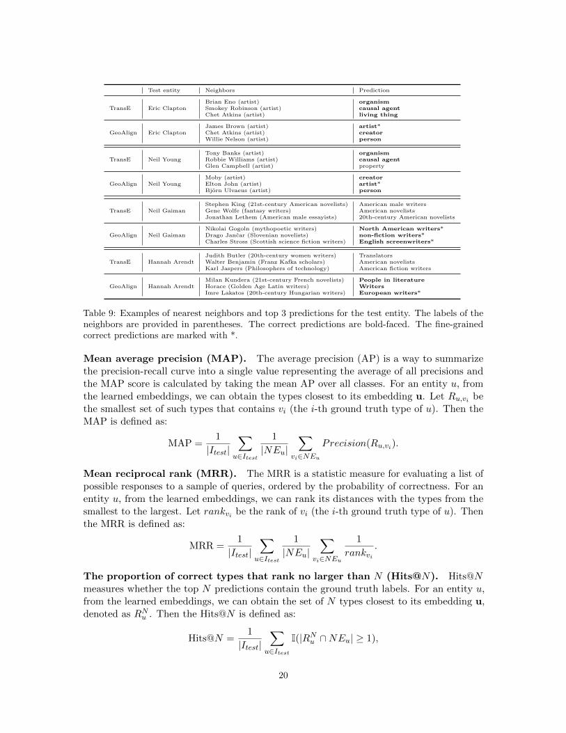
Table 9: Examples of nearest neighbors and top 3 predictions for the test entity. The labels of theneighbors are provided in parentheses. The correct predictions are bold-faced. The fine-grainedcorrect predictions are marked with *.

Mean average precision (MAP). The average precision (AP) is a way to summarizethe precision-recall curve into a single value representing the average of all precisions andthe MAP score is calculated by taking the mean AP over all classes. For an entity u, fromthe learned embeddings, we can obtain the types closest to its embedding u. Let Ru,vi bethe smallest set of such types that contains vi (the i-th ground truth type of u). Then theMAP is defined as:

MAP =1

|Itest|∑

u∈Itest

1

|NEu|∑

vi∈NEu

Precision(Ru,vi).

Mean reciprocal rank (MRR). The MRR is a statistic measure for evaluating a list ofpossible responses to a sample of queries, ordered by the probability of correctness. For anentity u, from the learned embeddings, we can rank its distances with the types from thesmallest to the largest. Let rankvi be the rank of vi (the i-th ground truth type of u). Thenthe MRR is defined as:

MRR =1

|Itest|∑

u∈Itest

1

|NEu|∑

vi∈NEu

1

rankvi.

The proportion of correct types that rank no larger than N (Hits@N). Hits@Nmeasures whether the top N predictions contain the ground truth labels. For an entity u,from the learned embeddings, we can obtain the set of N types closest to its embedding u,denoted as RNu . Then the Hits@N is defined as:

Hits@N =1

|Itest|∑

u∈Itest

I(|RNu ∩NEu| ≥ 1),

20


where I(|RNu ∩NEu| ≥ 1) is the indicator function.

D.3 Case Study

Our manifold alignment is on top of the pretrained TransE model and the hyperboloidembeddings. To have a more intuitive sense about the manifold alignment, in Table 9, wegive some examples of the nearest neighbors of the test entity in the aligned manifold aswell as the top 3 types predicted by GeoAlign. We also present the corresponding items ofTransE as a comparison. For TransE, the nearest neighbors are from its embedding space.The examples Eric Clapton and Neil Young are from YAGOwordnet while Neil Gaimanand Hannah Arendt are from wikiObjects. As we expect, TransE and manifold alignmentwhich leverages TransE both find the reasonable nearest neighbors. When looking into thetop 3 predictions of Eric Clapton and Neil Young , we see that although TransE predictscorrectly, it cannot get the fine-grained types. The most confident predictions of TransEare usually the general and rough types such as organism, living thing, while GeoAlignsuccessfully predict them as artist. For the test entities Neil Gaiman and Hannah Arendt ,which come from the more fine-grained and massive taxonomy wikiObjects, TransE cannotpredict correctly at the top 3 predictions, but GeoAlign successfully obtains the correctfine-grained types. The results show that GeoAlign not only outputs accurate predictionsbut also captures the hierarchy structure to some extent.

21

manifold alignment across geometric spaces for knowledge

Documents