manifold learning in computer vision
TRANSCRIPT

The Pennsylvania State University
The Graduate School
Department of Computer Science and Engineering
MANIFOLD LEARNING IN COMPUTER VISION
A Thesis in
Computer Science and Engineering
by
JinHyeong Park
c© 2005 JinHyeong Park
Submitted in Partial Fulfillmentof the Requirements
for the Degree of
Doctor of Philosophy
August 2005

We approve the thesis of JinHyeong Park.
Date of Signature
Rangachar KasturiProfessor of Computer Science and EngineeringThesis Co-AdviserCo-Chair of Committee
Hongyuan ZhaProfessor of Computer Science and EngineeringThesis Co-AdviserCo-Chair of Committee
Octavia I. CampsAssociate Professor of Computer Science and Engineeringand Electrical Engineering
Richard L. TutwilerSenior Research Associate of Applied Research Laboratory
Raj AcharyaProfessor of Computer Science and EngineeringHead of the Department of Computer Science and Engineering

iii
Abstract
Appearance based learning has become very popular in the field of computer
vision. In a particular system, a visual datum such as an image is usually treated as
a vector by concatenating each row or column. The dimension of the image vector is
very high, equal to the number of pixels of the image. When we consider a sequence of
images, such video sequences or images capturing an object from different view points,
it typically lies on a non-linear dimensional manifold, whose dimension is much lower
than that of the original data. When we know the structure of the non-linear manifold,
it can be very helpful in the field of computer vision for various applications such as
dimensionality reduction, noise handling, etc.
In the first part of this thesis, we propose a method for outlier handling and noise
reduction using weighted local linear smoothing for a set of noisy points sampled from
a nonlinear manifold. This method can be used in conjunction with various manifold
learning methods such as Isomap (Isometric Feature Map), LLE (Local Linear Embed-
ding) and LTSA (Local Tangent Space Alignment) as a preprocessing step to obtain a
more accurate reconstruction of the underlying nonlinear manifolds. Using Weighted
PCA (Principal Component Analysis) as a foundation, we suggest an iterative weight
selection scheme for robust local linear fitting together with an outlier detection method
based on minimal spanning trees to further improve robustness. We also develop an
efficient and effective bias-reduction method to deal with the “trim the peak and fill the
valley” phenomenon in local linear smoothing. Synthetic examples along with several real
iv
image data sets are presented to show that we can combine manifold learning methods
with weighted local linear smoothing to produce more accurate results. The proposed
local smoothing method has been applied to the image occlusion handling problem and
to the noise reduction problem for point-based rendering.
The second part of this thesis focuses on image occlusion handling utilizing man-
ifold learning. We propose an algorithm to handle the problem of image occlusion using
the Least Angle Regression (LARS) algorithm. LARS, which was proposed recently
in the area of statistics, is known as a less greedy version of the traditional forward
model selection algorithm. In other words, the LARS algorithm provides a family of
image denoising results from one updated pixel to all of the updated pixels. Using image
thresholding and the statistical model selection criterion of Akaike Information Crite-
rion (AIC), we propose a method for selecting an optimal solution among the family of
solutions that the LARS algorithm provides. Three sets of experiments were performed.
The first measured the stability of the optimal solution estimation method. The second
set showed the effects of subblock computation on performance. The last set applied
the occlusion handling algorithm to the noisy data cleaning problem, and compared it
to two other methods: Orthogonal projection with Weighted PCA and Robust PCA.
Experimental results showed that the proposed method yields better performance than
the other methods.
In the third part of this thesis, we propose a robust motion segmentation method
using the techniques of matrix factorization, subspace separation and spectral graph
partitioning. We first show that the shape interaction matrix can be derived using QR
decomposition rather than Singular Value Decomposition(SVD) which also leads to a

v
simple proof of the shape subspace separation theorem. Using the shape interaction
matrix, we solve the motion segmentation problems using spectral clustering techniques.
We exploit the multi-way Min-Max cut clustering method and provide a novel approach
for cluster membership assignment. We further show that we can combine a cluster
refinement method based on subspace separation with the graph clustering method which
improves its robustness in the presence of noise. The proposed method yields very good
performance for both synthetic and real image sequences.

vi
Table of Contents
List of Tables . . . . . . . . . . . . . . . . . . . . . . . . . . . . . . . . . . . . . . ix
List of Figures . . . . . . . . . . . . . . . . . . . . . . . . . . . . . . . . . . . . . x
Acknowledgments . . . . . . . . . . . . . . . . . . . . . . . . . . . . . . . . . . . xv
Chapter 1. Introduction . . . . . . . . . . . . . . . . . . . . . . . . . . . . . . . . 1
1.1 Organization of the Dissertation . . . . . . . . . . . . . . . . . . . . . 6
Chapter 2. Local Smoothing for Manifold Learning . . . . . . . . . . . . . . . . 8
2.1 Nonlinear Dimensionality Reduction using Manifold Learning . . . . 9
2.1.1 Isometric Feature Map (Isomap) . . . . . . . . . . . . . . . . 10
2.1.2 Local Linear Embedding (LLE) . . . . . . . . . . . . . . . . 11
2.1.3 Curvilinear Distance Analysis (CDA) . . . . . . . . . . . . . . 13
2.1.4 Local Tangent Space Alignment (LTSA) . . . . . . . . . . . . 14
2.1.5 Laplacian Eigenmaps and Spectral Techniques for Embedding
and Clustering . . . . . . . . . . . . . . . . . . . . . . . . . . 16
2.2 Weighted PCA . . . . . . . . . . . . . . . . . . . . . . . . . . . . . . 17
2.3 Selecting Weights for WPCA . . . . . . . . . . . . . . . . . . . . . . 20
2.4 Further Improvement for Outlier Handling using MST . . . . . . . . 23
2.5 Bias Reduction . . . . . . . . . . . . . . . . . . . . . . . . . . . . . . 27
2.6 Experimental Results . . . . . . . . . . . . . . . . . . . . . . . . . . . 29

vii
2.6.1 2D Spiral Curve Data . . . . . . . . . . . . . . . . . . . . . . 29
2.6.2 Experiments using 3D Swiss Roll Data . . . . . . . . . . . . 34
2.6.3 Smoothing 3D Points for Rendering . . . . . . . . . . . . . . 37
2.6.4 Face Images and Two Video Sequences (Human Walking and
Ballet) . . . . . . . . . . . . . . . . . . . . . . . . . . . . . . . 44
Chapter 3. Image Denoising Using LARS Algorithm . . . . . . . . . . . . . . . . 49
3.1 Problem Definition . . . . . . . . . . . . . . . . . . . . . . . . . . . . 51
3.1.1 Image Denoising using ℓ1 constraints . . . . . . . . . . . . . . 56
3.2 Image Denoising using LARS . . . . . . . . . . . . . . . . . . . . . . 59
3.2.1 Relationship between Image Denoising Objective Function and
Lasso . . . . . . . . . . . . . . . . . . . . . . . . . . . . . . . 60
3.2.2 Overview of LARS algorithm . . . . . . . . . . . . . . . . . . 61
3.3 The Optimal Solution Computation Using Thresholding and AIC . . 68
3.3.1 Statistical Model Selection Criteria . . . . . . . . . . . . . . . 68
3.3.2 Selecting the Optimal Solution Using Thresholding and AIC . 69
3.4 Improvement of the Computation Time . . . . . . . . . . . . . . . . 73
3.5 Sub-Block Computation Using Wavelets decomposition . . . . . . . . 76
3.5.1 Basic concept of Haar Wavelet Analysis . . . . . . . . . . . . 76
3.5.2 Decomposition of Images using Modified Haar Wavelet Analysis 79
3.6 Experiments . . . . . . . . . . . . . . . . . . . . . . . . . . . . . . . . 81
3.6.1 Performance of Optimal Solution Estimation . . . . . . . . . 81
3.6.2 Performance for Sub-Block Computation . . . . . . . . . . . . 82

viii
3.6.3 Occlusion Handling for Noisy Data . . . . . . . . . . . . . . . 85
Chapter 4. Spectral Clustering for Robust Motion Segmentation . . . . . . . . . 90
4.1 Matrix Factorization Method for Shape Recovery and Motion Seg-
mentation . . . . . . . . . . . . . . . . . . . . . . . . . . . . . . . . . 91
4.2 Multibody Motion Segmentation Algorithms . . . . . . . . . . . . . . 95
4.3 Constructing the Shape Interaction Matrix Using QR Decomposition 97
4.4 Motion Segmentation . . . . . . . . . . . . . . . . . . . . . . . . . . . 99
4.4.1 Spectral Multi-way clustering . . . . . . . . . . . . . . . . . . 99
4.4.2 Refinement of cluster assignment for motion segmentation . . 104
4.5 Experimental Results . . . . . . . . . . . . . . . . . . . . . . . . . . . 105
4.5.1 Synthetic Data . . . . . . . . . . . . . . . . . . . . . . . . . . 105
4.5.2 Real Video Sequences . . . . . . . . . . . . . . . . . . . . . . 107
Chapter 5. Summary and Conclusions . . . . . . . . . . . . . . . . . . . . . . . . 110
5.0.3 Contributions . . . . . . . . . . . . . . . . . . . . . . . . . . . 113
5.0.4 Future Works . . . . . . . . . . . . . . . . . . . . . . . . . . . 114
Appendix A. Computation of the Equiangular vector uA, w and AA . . . . . . 116
Appendix B. 2D Haar Wavelet Analysis . . . . . . . . . . . . . . . . . . . . . . . 118
References . . . . . . . . . . . . . . . . . . . . . . . . . . . . . . . . . . . . . . . . 120

ix
List of Tables
3.1 Reconstruction Error of the test images from the second row to the sev-
enth row of Fig. 3.11. ‖ · ‖2 represents ℓ2 norm. . . . . . . . . . . . . . . 84
3.2 Average reconstruction errors based on ℓ2 norm and their standard deviation
(inside the parenthesis). . . . . . . . . . . . . . . . . . . . . . . . . . . . . 87
4.1 An example of the matrix R. There are 10 points extracted from 3
objects. The last row shows the assigned cluster . . . . . . . . . . . . . 103
4.2 Misclassification rate (%) for the two synthetic sequences. The values
in parentheses are the standard deviation values. Method 1 is the k-
way Min-Max cut clustering discussed in Section 4.4.1 and Method
2 is the k-way Min-Max cut clustering plus the clustering refinement
using subspace projection discussed in Section 4.4.2. Multi-Stage is
the Multi-stage optimization proposed in [33]. . . . . . . . . . . . . . . . 106
4.3 Misclassification rate (%) for the real video sequences. The values in
parentheses are the standard deviation values. . . . . . . . . . . . . . . 108

x
List of Figures
2.1 WPCA results for various γ’s. Blue line denotes the first principal component
direction of the original PCA, and the other color lines denote those of WPCA
with different γ’s (cyan:γ=0.1, magenta:γ=0.5 and green:γ=1). Magenta line
is overlapped with green line in (a), and cyan line is overlapped with blue line
in (b). “X” mark denotes the weighted center after applying WPCA. . . . . . 26
2.2 An example of Minimum Spanning Tree (MST) . . . . . . . . . . . . . . . . 26
2.3 Shrinking Example. Green dots, red dots and blue dots are the original input
data points, the smoothing results at the iteration and the target manifold,
respectively. Parameters: k=30, γ=0.1; (a) Original input image. (b)&(c) are
the results without bias correction. (d)&(e) are results with bias correction. . . 29
2.4 Smoothing results for Gaussian noise data with different γ’s. Green dots are
the input data, and red dots are smoothing results. The first row shows the
results without MST outlier handling, and the second row shows those with
MST outlier handling. The parameter k is set to 30 and the number of iteration
to 10. . . . . . . . . . . . . . . . . . . . . . . . . . . . . . . . . . . . . . . 32
2.5 Smoothing results for outlier-overlaid data with different γ’s. The parameter k
is set to 30 and the number of iteration to 10. . . . . . . . . . . . . . . . . . 33
2.6 Smoothing results with different ks. γ is set to 0.1 and the number of iteration
to 10. . . . . . . . . . . . . . . . . . . . . . . . . . . . . . . . . . . . . . . 33
2.7 Plots of Swiss roll data . . . . . . . . . . . . . . . . . . . . . . . . . . . . . 36

xi
2.8 Original Gnome data . . . . . . . . . . . . . . . . . . . . . . . . . . . . . . 39
2.9 Original Santa data . . . . . . . . . . . . . . . . . . . . . . . . . . . . . . 39
2.10 Noisy Gnome data with Gaussian random noise, N (0, 2) . . . . . . . . . . . . 40
2.11 Smoothing results of noisy Gnome data in Fig. 2.10 . . . . . . . . . . . . . . 40
2.12 Noisy Gnome data with Gaussian random Noise, N (0, 4) . . . . . . . . . . . 41
2.13 Smoothing results of noisy Gnome data in Fig. 2.12 . . . . . . . . . . . . . . 41
2.14 Noisy Santa data with Gaussian random Noise, N (0, 3) . . . . . . . . . . . . 42
2.15 Smoothing results of noisy Santa data in Fig. 2.14 . . . . . . . . . . . . . . . 42
2.16 Noisy Santa data with Gaussian random Noise, N (0, 5) . . . . . . . . . . . . 43
2.17 Smoothing results of noisy Santa data in Fig. 2.16 . . . . . . . . . . . . . . . 43
2.18 Residual variances for each dimension after applying Isomap to face images. (a)
shows residual variances for original images without noise. kIsomap in (a) stands
for the number of neighbors for Isomap. (b)-(e) show the residual variance for
occlusion-overlaid cases (green line) and their smoothing results (blue line).
s× s, r% means a s× s size of noise patch is overlaid to r% of the data . . . . 46
2.19 (a) shows occlusion-overlaid face images in the size of 20 × 20 to 20% of the
data set. (b) shows the smoothing results of (a). . . . . . . . . . . . . . . . . 46
2.20 Residual variances for each dimension after applying Isomap. (a) shows residual
variances for original images without noise. (b)-(e) show the residual variances
for occlusion-overlaid cases. . . . . . . . . . . . . . . . . . . . . . . . . . . 47
2.21 (a) shows occlusion-overlaid human walking images in the size of 10×10 to 40%
of the data set. (b) shows the smoothing results of (a). . . . . . . . . . . . . 47

xii
2.22 Residual variances for each dimension after applying Isomap. (a) show residual
variances for original images without noise. (b)-(e) show the residual variance
for noise contamination cases. . . . . . . . . . . . . . . . . . . . . . . . . . 48
2.23 (a) shows occlusion-overlaid images in the size of 15 × 15 to 30% of the data
set. (b) shows the smoothing results of (a). . . . . . . . . . . . . . . . . . . 48
3.1 This curve represents a manifold of images including, x. The vertical axis and
the horizontal axis represent the occlusion pixels and the non-occlusion pixels
of the image x respectively . . . . . . . . . . . . . . . . . . . . . . . . . . . 52
3.2 Boat test image and its reconstruction images . . . . . . . . . . . . . . . . . 53
3.3 Fourteen Training boat images . . . . . . . . . . . . . . . . . . . . . . . . . 54
3.4 Plot of the boat images into 2D space. . . . . . . . . . . . . . . . . . . . . . 55
3.5 (a) |α| images computed by applying the LARS algorithm. (b) Binary images of
|α|’s. The white pixels represent a non-zero value. (c) Binary images after ap-
plying the thresholding algorithm to (a). (d) Reconstruction images by adding
α to the occlusion image . . . . . . . . . . . . . . . . . . . . . . . . . . . . 72
3.6 (a) The blue line and red dashed line represent the number of foreground pixels
and the sum of the absolute values of the foreground pixels, respectively, after
applying the thresholding algorithm (b) ℓ2 norm reconstruction error. . . . . . 72
3.7 Haar wavelet decomposition of an image. . . . . . . . . . . . . . . . . . 79
3.8 Modified Haar wavelet decomposition . . . . . . . . . . . . . . . . . . . 80
3.9 Occlusion images in the first row and their reconstruction Results in the second
row . . . . . . . . . . . . . . . . . . . . . . . . . . . . . . . . . . . . . . 82

xiii
3.10 The first row plots |FGi|’s and the second row plots their reconstruction error
through the iteration of the 5 test images in Fig. 3.9. The red dot indicates the
position of the selected optimal solution. . . . . . . . . . . . . . . . . . . . . 83
3.11 Image denoising results of face images. (a) Original images. (b) Occlu-
sion overlaid images of (a). (c) PCA reconstruction (d) LARS reconstruc-
tion without Haar wavelet decomposition. (e) ∼ (g) LARS reconstruction
by applying the proposed Haar wavelet decomposition of level 1 (4 sub-
bands, size of 32× 32), level 2 (16 subbands, size of 16× 16) and level 3
(64 subbands, size of 8× 8), respectively. . . . . . . . . . . . . . . . . . . 84
3.12 Selected reconstruction results of the face data, the human walking video se-
quence, and the ballet video sequence. (a) 10 selected occlusion images (b)
Reconstruction results of Proposed LARS algorithm, (c) Reconstruction results
of the Local Smoothing method proposed in [45], (d): Reconstruction results
of Robust PCA [15] . . . . . . . . . . . . . . . . . . . . . . . . . . . . . . 88
3.13 (a) 20 selected occlusion overlaid images from video sequence. (b) LARS
reconstruction. (c) Absolute images between (a) and (b). (d) RPCA
reconstruction. (e) Absolute images between (a) and (d). . . . . . . . . 89
4.1 The two synthetic video sequences used in [32] and [33] respectively.
(a). 20 green dots are background pixels and 9 foreground points (b). 24
background points and 14 foreground points. The foreground pixels are
connected with lines. . . . . . . . . . . . . . . . . . . . . . . . . . . . . . 105

xiv
4.2 Real video sequences with the feature points. 1st row: video1, 2nd row:
video2, 3rd row: video3, 4th row: video4 (foreground feature points in
video1 are overlaid onto video2). Red dots correspond to the background
while green dots correspond to the foreground. The yellow cross marks
in video4 represent the foreground feature points of video1 . . . . . . . 109
4.3 Graph for misclassification rate. Graph of video1 is not depicted here
because all of the methods perform perfectly. Method 1: Dashed-dot
blue line, Method 2: Red line and Multi-Stage: Dashed green line . . 109

xv
Acknowledgments
First of all, I praise and give my thank from deep inside my heart to God who
has guided me through my study. He listened to my cry and he was always with me
whenever I was wandering in the desert without hope. When I fall on the ground, he
raised me. When I couldn’t feel any hope he blowed a breeze of help to me. Thank you,
God.
I would like to express my heartfelt and sincere thanks to my co-advisors and the
co-chairman of my thesis committee, Prof. Rangachar Kasturi and Prof. Hongyuan Zha,
for their guidance and support over the course of my research. I also appreciate the other
committee members, Dr. Octavia I. Camps and Dr. Richard L. Tutwiler, their useful
suggestions and valuable comments on the thesis. I would like to thank Prof. Jesse L.
Barlow and Dr. Robert T Collins for their encouragement and intesest in my work.
My thanks also goes to my colleagues in Computer Vision group and other former
graduate students in the group. It was thank the Korean graduate students in my
departments for their concern and encouragement. I would like to thank the members
of PSU Korean Soccer Club. My life in State College was enjoyable because I could play
soccer with great friends every Saturday. It was very helpful to keep my body strong
enough to pursue my research.
I would like to thank Pastor Sang-kee Eun and Pastor Ju-Young Lee at the State
College Korean Church for teaching and guiding me to know the love of the Christ Jesus.
I also thank all the brothers and sisters in the church who encouraged me whenever I

xvi
was depressed, and prayed for me whenever I need help. My thanks also goes to Pastor
David Alas for his help in editing my thesis.
My thank also goes to my mother-in-law and father-in-law for there love and
support. Especially, I appreciate my mother-in-law, Bokja Jeon, who always prayed for
my family and my research. I would like thank my father Chung-Su Park and my mother
Guja Han for their unconditional love and support . I am very proud of being your the
first son. You are the best father and the best mother on earth.
Finally, I truly thank my wife, Jayeoun Lim, for her love and support, and her
patience during the period of time it took me to pursue this research. My son, Daniel
Jaemin Park, it was my best time on earth when you were born, June 6th, 2002. You,
my beautiful wife and adorable son, are the best motivation of my study.

1
Chapter 1
Introduction
Manifold learning represents a novel set of methods for nonlinear dimension reduc-
tion emphasizing simple algorithmic implementation and avoiding optimization problems
prone to local minima [59, 50, 69]. It has applications in several areas of computer vision
such as image interpolation and tracking. At the pixel level, a set of images such as a
collection of faces can be represented as high-dimensional vectors, but their intrinsic di-
mension is usually much smaller than the ambient feature space. Capturing this intrinsic
dimension from a set of samples is of paramount importance in computer vision appli-
cations. This is evident given the increasing interest in subspace-based methods such as
Principal Component Analysis (PCA) [30], Independent Component Analysis (ICA) [27],
and Non-linear Matrix Factorization (NMF) [36], just to name a few. Furthermore, these
generally linear methods have recently been joined by several non-linear dimensionality
reduction methods such as Isomap (Isometric feature mapping) [59, 58], LLE (Local
Linear Embedding) [50] and LTSA(Local Tangent Space Alignment)[69]. One chief ad-
vantage of the newer methods is that they can successfully compute dimension reduction
for data points sampled from a nonlinear manifold.
In many real-world applications with high-dimensional data, the components of
the data points tend to be correlated with each other, and in many cases the data points

2
lie close to a low-dimensional nonlinear manifold. Discovering the structure of the man-
ifold from a set of data points possibly with noise represents a very challenging unsu-
pervised learning problem [50, 18, 51, 59]. But once discovered, these low-dimensional
structures can be used for classification, clustering, and data visualization. Traditional
dimensionality reduction techniques such as principal component analysis (PCA), factor
analysis and multidimensional scaling usually work well when the underlying manifold
is a linear (affine) subspace[26]. However, they can not, in general, discover nonlinear
structures embedded in the set of data points.
Recently, there has been a growing interest in developing efficient algorithms
for constructing nonlinear low-dimensional manifolds from sample data points in high-
dimensional spaces emphasizing simple algorithmic implementation and avoiding opti-
mization problems prone to local minima [50, 59]. Two main approaches are the Isomap
methods [18, 59] and the local linear embedding methods (LLE and LTSA) [50, 69].
In the first method, pairwise geodesic distances of the data points with respect to
the underlying manifold are estimated, and classical multi-dimensional scaling is used to
project the data points into a low-dimensional space that best preserves these geodesic
distances. The latter method follows a long tradition, starting with self-organizing maps
(SOM) [34], principal curves/surfaces [25] and topology-preserving networks [41, 8]. The
key idea is that the information about the global structure of a nonlinear manifold can be
obtained from carefully analyzing the interactions of the overlapping local structures. In
particular, the local linear embedding (LLE) method constructs a local geometric struc-
ture that is invariant to translations and orthogonal transformations in a neighborhood
of each data point, and seeks to project each data point into a low-dimensional space that

3
best preserves these local geometries [50, 51]. LTSA[69] uses the tangent space in the
neighborhood of each data point to represent the local geometry, and then aligns those
local tangent spaces to construct a global coordinate system for the nonlinear manifold.
Similar to PCA, however, these manifold learning methods are still quite sensitive to
outliers. The focus of this research is the development of an outlier handling and noise
reduction method that can be used with those nonlinear methods as a preprocessing
procedure to obtain a more accurate reconstruction of the underlying nonlinear man-
ifold. More importantly, outlier handling and noise reduction will reduce the chances
of short-circuit nearest neighbor connections and therefore help to better preserve the
topological/geometric structures of the manifold in a neighborhood graph constructed
from a finite set of noisy sample points.
Computer vision has recently received a lot of attention due to the significant
increase of visual data, as well as the improvement of computer processing power and
memory capacity. Computer vision tasks such as face recognition or human activity
recognition are very challenging when the visual data is corrupted by noise. Hence
image denoising is an important pre-processing step in computer vision applications and
has been studied extensively [9] [15] [7] [43]. The usual approach to image denoising
is to project the image orthogonally onto the subspace (simple smoothing) computed
using a training data set. When we apply the proposed local smoothing method to
image occlusion handling, it also computes the local tangent space of an given occlusion
image and projects the image orthogonally onto the local tangent space. This approach
has several shortcomings especially when only a part of the image is corrupted, since
all the pixel values are changed after orthogonally projecting the noisy image onto the

4
subspace. Tsuda et al. [63] proposed an image denoising method to identify the noisy
pixels by ℓ1 norm penalization and to update only the identified noisy pixels. It is well
known that ℓ1 norm penalization yields a sparse solution. Therefore, the main purpose
of using ℓ1 norm penalization in [63] is to select only noisy pixels. They construct a
Linear Programming (LP) problem with ℓ1 constraints to identify and update the noisy
pixels simultaneously.
This approach has a significant advantage over the other methods in terms of re-
construction error since it only updates a small part of the image pixels without touching
the other pixels. However, this method needs a parameter to control the fraction of the
updated pixels. The higher the value of this parameter, the greater the number of pixels
that are updated. We propose a new image occlusion handling method using the Least
Angle Regression (LARS) [19] algorithm. LARS was originally proposed as a feature
selection method for the regression problem, which claims to be a less greedy version
of the original forward feature selection method. LARS is based on the iteration and
provides all the solutions (feature selection) by adding one feature at each iteration at a
cheap cost in computation time.
To this end, we first show that the image occlusion handling problem can be
converted into a regression problem. In this new regression problem, each covariate cor-
responds to a pixel. Secondly, we apply the LARS algorithm to the problem to obtain all
the solutions (from one updated pixel to all of the updated pixels). Actually, the ℓ1 con-
straints which were used in [63] are not necessary when we use LARS algorithm because
the purpose of the ℓ1 constraint is to compute a sparse solution, and LARS provides all

5
the possible sparse solutions. Finally, we select the optimal solution from among the fam-
ily of solutions that the LARS algorithm yields using an image thresholding technique
and a statistical model selection method. Thus, the proposed image occlusion handling
method would need no parameter. We also discuss sub-block computation using Wavelet
decomposition to further improve the computation time.
Afterwards, we discuss motion segmentation using matrix fatorization. Matrix
factorization methods have been widely used for solving the motion segmentation prob-
lems [21] [28] [29] [64] [31] [32] [33] [66] and 3D shape recovering problems [12] [62] [11].
The factorization method proposed by Tomasi and Kanade [61] was for the case of a
single static object viewed by a moving camera. The basic idea of this method was
to factorize the feature trajectory matrix into the motion matrix and the shape ma-
trix, providing the separation of the feature point trajectories into independent motions.
Singular Value Decomposition (SVD) is used for this factorization.
Costerira and Kanade proposed a multi-body factorization method for indepen-
dent moving objects that builds upon the previous factorization method [14]. The shape
interaction matrix was proposed for grouping feature points into independent objects.
Given a set of N feature points tracked through F frames, we can construct a fea-
ture trajectory matrix P ∈ R2F×N where the rows correspond to the x or y coordinates
of the feature points in the image plane and the columns correspond to the individual
feature points. Motion segmentation algorithms based on matrix factorization [31] first
construct a shape interaction matrix Q by applying the singular value decomposition
(SVD) to the feature trajectory matrix P. Under the noise-free situation, the shape
interaction matrix Q can be transformed into a block diagonal matrix by a symmetric

6
row and column permutation thereby grouping the feature points of the same object into
a diagonal block.
If the trajectory matrix P is contaminated by noise, however, the block diagonal
form of Q no longer holds, and the methods such as the greedy technique proposed in[14]
tend to perform rather poorly. Recently there has been much research proposed that
specifically addresses this problem [32] [64] [21] [28] [64] [31] [66].
We have developed a novel robust factorization method using the techniques of
spectral clustering. We mathematically show that the shape interaction matrix can be
constructed by applying QR decomposition with pivoting instead of SVD. It is widely
known that QR decomposition is more stable and efficient than SVD. We applied the
spectral graph partitioning algorithm to the shape interaction matrix for clustering the
feature points into independent moving objects.
1.1 Organization of the Dissertation
Chapter 2 deals with a noise handling method for manifold learning. WPCA and
the weight selection are discussed in Section 2.2 and Section 2.3 respectively. The MST-
based outlier handling follows in Section 2.4. We propose a new bias correction method
in Section 2.5. Experimental results are discussed in Section 2.6.
Chapter 3 examines a method for image occlusion handling using the LARS al-
gorithm. We define the problem in Section 3.1, and the LARS algorithm is summarized
in Section 3.2.2. Optimal solution computation using a thresholding technique and a

7
statistical model selection criterion is proposed in Section 3.3. Improvement of com-
putation time is discussed in Section 3.4. Sub-block computation using Haar Wavelet
decomposition is proposed in 3.5. Experimental results are shown in Section 3.6.
Chapter 4 discusses motion segmentation using matrix factorization and spectral
graph partitioning. Previous work in the area of multi-body motion segmentation is
discussed in Section 4.2. Section 4.3 is devoted to a proof showing that the shape
interaction matrix can be computed using QR decomposition. Motion segmentation
based on spectral relaxation k-way clustering and subspace separation is described in
Section 4.4. Experiment results are shown in Section 4.5.
Chapter 5 provides the summary of the dissertation and discusses future work.

8
Chapter 2
Local Smoothing for Manifold Learning
In this chapter, we focus on noise reduction and outlier handling by exploiting
the basic idea of weighted local linear smoothing. The techniques we used are simi-
lar in spirit to local polynomial smoothing employed in non-parametric regression [38].
However, since in our context, we do not have the response variables, local smoothing
needs to employ techniques other than least squares fitting. Since we are interested in
modeling high-dimensional data, and therefore in local smoothing we try to avoid more
expensive operations such as approximating the Hessian matrices when we carry out
bias reduction. Furthermore, we apply local smoothing in an iterative fashion to further
improve accuracy.
We assume that F is a d-dimensional manifold in an m-dimensional space with
unknown generating function f(τ), τ ∈ Rd, and we are given a data set of N vectors
xi ∈ Rm, i = 1, 2, . . . , N , generated from the following model,
xi = f(τi) + ǫi, i = 1, . . . , N, (2.1)
where τi ∈ Rd with d < m, and ǫi’s represent noise. The goals of nonlinear manifold
learning are to 1) construct the τi’s from the xi’s; and 2) construct an approximation
of the generating function f(τ) [69]. In the local smoothing method we will discuss, the
nonlinear manifold F is locally approximated by an affine subspace. Before applying

9
a manifold learning method, we propose to carry out a local smoothing procedure as
follows. For each sample point xi, i = 1, 2, . . . , N , we compute its k nearest neighbor
sample points. The sample point xi is then examined to see if it is located in the middle
of two or more patches of the manifold using outlier detection based on a Minimum
Spanning Tree (MST). If it is we move xi to one of the patches, otherwise we compute
an affine subspace using Weighted PCA (WPCA) from the k nearest neighbors, and
project the xi to this affine subspace. After projecting (or moving) all the sample points,
we correct their bias, and then the above steps are iterated several times. Experiments
were conducted using synthetic two dimensional (2D) data sets and three dimensional
(3D) data sets. The proposed local smoothing method was also applied to point-based
rendering problem in the field of Computer Graphics, and to an image occlusion handling
problem.
2.1 Nonlinear Dimensionality Reduction using Manifold Learning
In this section, we review five important nonlinear dimensionality algorithms:
Isomap, LLE, CDA, LTSA and Laplacian Eigenmaps. Let us assume that the d-dimensional
manifold F embedded in anm-dimensional space (d < m) can be represented by a vector-
valued multivariate function
f : C ⊂ Rd → Rm,
where C is a compact subset of Rd with open interior. We are given a set of data points
x1, · · · , xN with xi ∈ Rm, which are sampled possibly with noise from the manifold,
i.e.,

10
xi = f(yi) + ǫi, i = 1, . . . , N, (2.2)
where ǫi represents noise. By dimension reduction we mean the estimation of the
unknown lower dimensional feature vectors yi’s from the xi’s, realizing the objective of
(nonlinear) dimensionality reduction of the data points.
2.1.1 Isometric Feature Map (Isomap)
Isometric Feature Map (Isomap) was a novel nonlinear dimensionality reduction
method proposed by Tenenbaum et. al. [59] which finds the subspace that preserves
the geodesic interpoint distances. This algorithm has three steps. The first step is to
construct a neighborhood graph by determining the neighborhood points of each input
point on the manifold M , based on the distances dx(i, j) between two pairs of points,
xi and xj in the input space X. Two simple methods are considered to determine the
criterion of neighborhood: k-nearest neighbors and points within some fixed radius ǫ.
These neighborhood relations are represented as a weighted graph G over the data points,
with edges of weight dx(i, j) between neighboring points.
In the second step, the algorithm estimates the geodesic distance dM (i, j) between
all pairs of points on the manifold M by computing their shortest path distance dG(i, j).
A simple method to compute the distance dG(i, j) can be summarized as follows.
• Initialization
dG(i, j) =
dX (i, j) if i, j are linked by an edge in G
∞ otherwise

11
• Update dG(i, j) (Floyd’s algorithm)
dG(i, j) = min dG(i, j), dG(i, k) + dG(k, j), k = 1, 2, ..., N.
Re-iterate this update procedure until no further updates occur.
The final step applies classical Multidimensional Scaling (MDS) to the matrix of
graph distances dG(i, j) by constructing an embedding of the data in a d-dimensional
Euclidean space Y that best preserves the manifold’s estimated intrinsic geometry.
A continuous version of Isomap, called Continuum Isomap, was proposed in [68].
Continuum Isomap computes a set of eigenfunctions that forms the canonical coordinates
of the Euclidean space up to a rigid motion for a nonlinear manifold that can be isomet-
rically embedded onto the Euclidean space. This manifold learning in the continuous
framework is reduced to an eigenvalue problem of an integral operator.
2.1.2 Local Linear Embedding (LLE)
Local Linear Embedding (LLE) was proposed by Roweis et. el. [50] [53]. LLE
is an unsupervised learning algorithm that computes low-dimensional, neighborhood-
preserving embedding of high-dimensional input data. LLE maps its input data into
a single global coordinate system of lower dimensionality, and its optimizations do not
involve local minima. The LLE algorithm can be summarized as follows.

12
Suppose that the data consists of N real vectors vecXi ∈ ℜd, sampled from some
underlying manifold. The first step computes the weightsWis to minimize reconstruction
error specified in Equation2.3.
E(W ) =n
∑
i
‖xi −k
∑
i=1
w(i)j xi
N(j)‖2 (2.3)
where xiN(1)
, · · · , xiN(k)
are the neighborhood points of xi, and ‖ · ‖2 represents
ℓ2 norm. The function reflects how well each xi can be linearly reconstructed in terms of
its local neighbors. To compute the weights W(i)j the cost function should be minimized
subject to two constraints. First, each data point xi is reconstructed only from its
neighbors , enforcingW(i)(j)
= 0 if xi does not belong to the set of neighbors ofXi. Second,
the sum of the weights associated with each point should be one, i.e.,∑
jWij
= 1. In
particular, the same weights Wij that reconstruct the i− th data point in D dimensions
should also reconstruct its embedded manifold coordinates in d dimensions, where d < D.
In the second step, LLE constructs a neighborhood-preserving mapping based on
the above idea.
Φ(Y ) =
n∑
i
‖yi −k
∑
i=1
w(i)j YN(j)‖2 (2.4)
This cost function, similar to Eq. 2.3, is based on locally linear reconstruction
errors. The function estimates local coordinates, y1, · · · , yn in d dimensional manifold
space by fixing the weights computed in Eq. 2.3.

13
2.1.3 Curvilinear Distance Analysis (CDA)
The CDA [37] shares the same metrics with Isomap. The only difference is that
Isomap exploits the traditional MDS for projection from d-dimensional space (original
data space) to p-dimensional space(projection space), while CDA works with neural
methods derived from the Curvilinear Component Analysis(CCA) [16].
The error function of CDA is written as:
ECDA =n
∑
i=1
n∑
j=1
(δdij− dp
ij)2F (dp
ij) (2.5)
where δpij and d
pij are respectively the curvilinear distance in the data space and
the Euclidean distance in the projection space between the i − th and j − th points.
The factor F (dpij , λd) is generally chosen as a bounded and monotonically decreasing
function in order to favor local topology conservation. Decreasing exponential, sigmoid
or Lorentz functions are all suitable choices. A simple step function shown in Eq. 2.6
can also be used for the factor F (dpij , λd).
F (dpij
) =
1 if dpij ≤ λd
0 otherwise
(2.6)
The algorithm of CDA can be summarized in five steps:
1. Apply vector quantization on the raw data.
2. Compute k- or ǫ-neighborhoods and link neighboring prototypes.
3. Compute distances,D, using Dijkstra’s algorithm.

14
4. Optimize ECDA by stochastic gradient descent, in order to get coordinates for the
prototypes in the projection space
5. Run a piecewise linear interpolator to compute the projection of original data
points (this step is not necessary if step 1 was skipped).
From a theoretical point of view, there are two main differences between CDA and
Isomap. The first is the way they determine landmark points (or prototypes). The second
is the way they compute low-dimensional coordinates. The Isomap exploits classical
MDS, whereas the CDA optimizes the energy function in Eq. 2.5 using gradient decent
or stochastic gradient descent. The Isomap shows stronger mathematical foundation,
and yields the coordinates simultaneously. The CDA is based on the neural networks
and can converge to local minima based on the initial parameters, F and learning rate.
However, if the two parameters are well adjusted, CDA can find useful projections. It
can project not only the training data but also new data using interpolation method.
2.1.4 Local Tangent Space Alignment (LTSA)
LTSA was proposed by Zhang and Zha [69]. The basic idea is to use the tangent
space in the neighborhood of a datum point to represent the local geometry, and then
align those local tangent spaces to construct the global coordinate system for the nonlin-
ear manifold. The local tangent space provides a low-dimensional linear approximation
of the local geometric structure of the nonlinear manifold. It preserves the local coordi-
nates of the data points in the neighborhood with respect to the tangent space. Those
local tangent coordinates will be aligned in the low dimensional space by different local

15
affine transformations to obtain a global coordinate system. Given N m-dimensional
sample points sampled possibly with noise from an underlying d dimensional manifold,
it produces N d-dimensional coordinates T ∈ RdxN for the manifold constructed from k
local nearest neighbors.
Let Xi = [xi1, · · · , xik] be a matrix consisting of its k-nearest neighbors including
xi. First, compute the best d-dimensional affine subspace approximation for the data
points in Xi.
minx,Θ,Q
k∑
j=1
∥
∥
∥xij− (x+Qθj)
∥
∥
∥
2= minx,Θ,Q
∥
∥
∥Xi − (xeT +QΘ)
∥
∥
∥
2
where Q is of d columns and is orthonormal, and Θ = [θ1, . . . , θk].
Next, compute the d-dimensional global coordinates y1, · · · , yN for the local co-
ordinates of θa1, . . . , θk. Actually, y1, · · · , yN is the target coordinates for x1, · · · , xN .
To preserve as much of the local geometry in the low-dimensional feature space,
we seek to find yi and the local affine transformations Li to minimize the reconstruction
errors ǫ(i)j , i.e.,
∑
i
‖Yi(I −1
keeT )− LiΘi‖2, (2.7)
where Yi = [yi1, · · · , y1k].

16
2.1.5 Laplacian Eigenmaps and Spectral Techniques for Embedding and
Clustering
The method proposed in [6] [5] is based on the fact that Laplacian of a graph
obtained from data points may be viewed as an approximation to the Laplace-Beltrami
operator defined on the manifold. It has strong connections to the spectral clustering
algorithm developed in machine learning and computer vision [55] [23] [67].
Given N input points xiNi=1∈ Rm, we can construct a weighted graph with N
nodes, one for each point, and the set of edge connecting neighboring points to each
other. The algorithm is summarized as follows:
1. The first step is to put an edge between nodes i and j if xi and xj are close to each
other. We can simply think about “closeness” in two ways: k nearest neighbors
and ǫ-distance neighborhoods.
2. The second step is to determine the weights of the edges using one of two methods.
The first method is to simply assign Wij = 1 if and only if vertices i and j are
connected by an edge. Or, alternatively, you can use the heat kernel equation
below.
Wij = exp(−‖ xi − xj ‖2
σ)
3. Then, by computing d eigenvectors y1 · · · yd corresponding to the d smallest eigen-
values, whose eigenvalues are greater than zero, we can address the eigenvec-
tor problem Ly = λDy where D = diag(d1, · · · , dN ), di =∑Nj=1
Wij , L =

17
D − W which is the Laplacian matrix. The y1 · · · yd are the orthogonal basis
of d-dimensional manifold space.
2.2 Weighted PCA
A number of robust methods exists in the literature to deal with outlier problems,
especially in the statistics community: M-estimators [20], Least Median of Squares [49]
and so on. These methods were applied to computer vision problems, and a number
of variations were published to compute robust linear subspaces despite the presence of
outliers [65, 15, 56]. The weighted PCA (WPCA) we are presenting is similar to the
ideas of robust M-estimation. Since we only consider object-level outliers, our version of
WPCA has a closed-form solution. With both object-level and feature-level outliers, the
WPCA problem requires an optimization problem to be solved in an iterative fashion,
see [15] for example. To this end, for each sample point xi in the given data set, let
Xi = [xi1, . . . , xik
] be a matrix consisting of its k-nearest neighbors in terms of the
Euclidean distance. We can fit a d-dimensional affine subspace to the columns in Xi by
applying PCA to Xi. Since one of the goals of local smoothing is to reduce the effects of
outliers, we need to develop more robust version of PCA. Our basic idea is to incorporate
weighting to obtain a weighted version of PCA (WPCA).
Now, in the above example, we want to fit these k-nearest neighbors using an
affine subspace parameterized as c+Ut, where U ∈ Rm×d forms the orthonormal basis
of the affine subspace, c ∈ Rm gives the displacement of the affine subspace, and t ∈ Rd
represents the local coordinate of a vector in the affine subspace. To this end, we consider

18
the following weighted least squares problem:
minc, {ti}, UTU=Id
k∑
i=1
wi‖xi − (c+ Uti)‖2, (2.8)
where w1, · · · , wk are a given set of weights which will be discussed in the next sec-
tion. We denote X = [x1, · · · , xk] and T = [t1, · · · , tk]. The weight vector and the
corresponding diagonal matrix are defined, respectively, as
w = [w1, · · · , wk]T , D = diag(
√w1, · · · ,
√wk)
The following theorem characterizes the optimal solution to the weighted least
squares problem in (2.8)
Theorem 2.1. Let xw =∑
iwixi/∑
iwi be the weighted mean of x1, · · · , xk, and
let u1, · · · , uk be the largest left singular vectors of (X − xweT )D, where e is the k-
dimensional column vector of all ones. Then an optimal solution of the problem (2.8) is
given by
c = xw, U = [u1, · · · , uk], ti = UT (xi − xw).
Proof. Let
E = (X − (ceT + UT ))D
be the weighted reconstruction error matrix. Using v to denote the normalized vector of
w
√w = [
√w1, · · · ,
√wk]
T , v =√w/‖√w‖2,

19
we rewrite the error matrix E as
E = EvvT + E(I − vvT ).
Because DvvT = weTD/(eTw), we have that
EvvT = (X − (ceT + UT ))DvvT
=(
(xw − c)eT − UTweT /(eTw))
)
D
and
E(I − vvT ) = (X − (ceT + UT ))D − EvvT
=(
X − (xweT + UT )
)
D
with T = T (I − weT /(eTw)). Clearly, E = E(I − vvT ) is the reconstructed error
matrix corresponding to the feasible solution (xw, T ) to (2.8). Since ‖E‖F ≤ ‖E‖F and
E√w = 0, we can conclude that an optimal solution of (2.8) should have an error matrix
E satisfying E√w = 0. With this condition, we have
Xw = XD√w = (ceT + UT )D
√w = (ceT + UT )w.
It follows that
c = xw − Uα, α = Tw/eTw,

20
and
X − (ceT + UT ) = X − (xw + U(T − αeT )).
With an abuse of notation, denoting (T − αeT ) by T , the optimization problem (2.8)
reduces to
min{ti},UTU=Id
‖(X − xweT )D − UTD‖F .
The optimal solution, as given by the Singular Value Decomposition (SVD) of
matrix (X − xweT )D, is
U = Ud, TD = UTd
(X − xweT )D.
It follows that T = UTd
(X − xweT ), completing the proof.
Thus, the sample point xi is projected to x∗i
as
x∗1
= xw + UUT (x1 − xw).
This projection process is done for each of the sample points in {x1, . . . , xN}.
2.3 Selecting Weights for WPCA
In this section, we consider how to select the weights to be used in WPCA. Since
the objective of introducing the weights is to reduce the influence of the outliers as much
as possible when fitting the points to an affine subspace, ideally the weights should be

21
chosen such that wi is small if xi is considered as an outlier. Specifically, we let the
weight wi be inversely proportional to the distance between xi and an ideal center x∗.
Here x∗ is defined as the mean of a subset of the points in which outliers have been
removed. The ideal center x∗, however, is unknown. We will use an iterative algorithm
to approximate x∗ starting with the mean of the sample points.
To begin, we consider weights based on the isotropic Gaussian density function
defined as
wi = c0 exp(−γ‖xi − x‖2), (2.9)
where γ > 0 is a constant, x an approximation of x∗, and c0 the normalization
constant such that∑ni=1
wi = 1. Other types of weights discussed in [38] can also be
used.
Our iterative weight selection procedure for a given set of sample points xi1, . . . , xik
is structured as follows: Choose the initial vector xw(0) as the mean of the k vectors
xi1, . . . , xik, and iterate until convergence using the following:
1. Compute the current normalized weights, w(j)i = cj exp(−γ‖xi − xw(j−1)‖2).
2. Compute a new weighted center xw(j) =
∑ki=1
w(j)i xi.
Initially, we can choose x as the mean of all the k sample points {xi}. as an
approximation to the ideal center x∗. The existence of outliers can render the mean x
quite far away from x∗. Then we update x by the weighted mean xw =∑
wixi, using
the current set of weights given by (2.9), and compute a new set of weights by replacing
22
x by xw in (2.9). The above process can be carried out in several iterations. We now
present an informal analysis to illustrate why the iterative weight selection process can
be effective at down-weighting the outliers. Consider the simple case where the data set
of k + ℓ samples has several outliers x1, · · · , xℓ that are far away from the remaining
set xℓ+1, · · · , xℓ+k which are relatively close to each other. We also assume ℓ ≪ k.
Denote x0 the mean of all ℓ + k sample points and x the mean of the sample points
xℓ+1, · · · , xℓ+k. It is easy to see that
x0 =1
ℓ+ k
(
ℓ∑
i=1
xi + kx)
= x+ δ, δ =1
ℓ+ k
ℓ∑
i=1
(xi − x).
If ‖δ‖ ≫ ‖xj − x‖ for j = ℓ+1, · · · , ℓ+k, we have ‖xj − x0‖2 ≈ ‖δ‖2. Therefore,
for j = ℓ+1, · · · , ℓ+k, wj = c0 exp(−γ‖xj−x0‖2) ≈ c0 exp(−γ‖δ||2). On the other hand,
since ‖xi − x||2 ≫ ‖δ‖2 for i ≤ ℓ, we have wi = c0 exp(−γ‖xi − x0||2) ≈ 0. If ‖δ‖ is not
large compared with the distances between x and the clustered points xℓ+1, · · · , xℓ+k,
we also have ‖xi − x0‖ ≈ ‖xi − x‖ ≫ ‖xj − x‖ ≈ ‖xj − x0‖ for i ≤ ℓ < j. This implies
wi ≈ 0 and wj ≈ constant. Therefore, recalling that the weight set is normalized such
that∑
wi = 1, we conclude that w0 ≈ 0, i ≤ ℓ, wi ≈ 1k , i > ℓ. Therefore, xw ≈ x and
the updated weights wi have the effect of down-weighting the outliers.
We have not carried out a formal analysis of the above iterative process. Based
on several simulations, the sequence {xw(j)}, in general, seems to converge fairly fast.

23
2.4 Further Improvement for Outlier Handling using MST
In most situations, WPCA with the above weight selection scheme can handle
noise and outliers quite well. However, it is not easy for WPCA to handle outliers
located between two or more patches of a manifold as shown in Fig. 2.1-(b).
Fig. 2.1 depicts two examples of WPCA for various γ’s. In case (a), we present
a set of outliers under which WPCA performs quite well. The weights of the outliers
become close to zero when we increase the value of γ and the first principal axis is
computed correctly using WPCA (the green line or the red line). In Fig. 2.1-(b), the
weight selection method yields non-negligible weights for the two outliers lying between
the two patches of a manifold and almost zero for weights associated with the other
points of the patches for a large value of γ. The first principal axis becomes the green
line with γ = 1 see Fig. 2.1-(b).
We will now show that we can improve the performance of local smoothing further
by using Minimum Spanning Tree (MST). The key observation is that if a point xi is an
outlier as shown in Fig. 2.1-(b), the distance between the outlier point and the nearest
patch is much greater than the distances between two near-by points in a patch.
A spanning tree for a connected undirected weighted graph G is defined as a
sub-graph of G that is an undirected tree and contains all the vertices of G [4]. A
minimum spanning tree (MST) for G is defined as a spanning tree with the minimum
sum of edge weights. Suppose that we examine an arbitrary sample point, say xi, and
without loss of generality let X = {x1, ..., xk} denote the set of k-nearest neighbors of

24
xi. The MST-based outlier detection procedure proceeds as follows. First, we com-
pute a weighted Minimum Spanning Tree (MST) using X = {x1, ..., xk}. We define
an undirected, weighted, fully connected graph G = (V,E,W ), where V = {x1, ..., xk},
E = {e12, e13, ...e(k−1)k} and W = {w(e12), w(e13), ..., w(e(k−1)k)}. An element in E,
eab , stands for an edge associated with xa and xb, and w(eab) is the Euclidean distance
between the two vertices.
An MST algorithm such as Prim’s algorithm [4] provides a k − 1 edge list, E′
=
{..., e′
ia, e
′
ib, ...} where we assume e
′
iaand e
′
ibare the two edges associated with xi, which
spans all the points in X with the minimum total edge weights1. After obtaining the
MST, we compute the average weight (meanw) of the MST. If the maximum edge weight
associated with xi is much greater than the average edge weight, we divide the MST
into two subgraphs G1 = (V1, E1) and G2 = (V2, E2). This is done by disconnecting
one of the edges, e′
iaor e
′
ib, whose weight is greater than the other as shown in Fig. 2.2.
In the next step, we examine whether or not the point is far from the other patch. Let
us assume G1 contains xi. We compare the maximum edge weight in G1 to the average
edge weight (meanw). If the edge weight is also much greater than the average weight,
the point is determined as the outlier between the two patches.
If a point, xi is diagnosed as an outlier between two local patches, it is moved in
the direction of one of the patches without projecting it onto its tangent space according
to the following equation:
1In this section, we only consider the outliers between two patches of a manifold (Fig. 2.1-(b))because WPCA can handle the other type of outliers shown in Fig. 2.1-(a) quite well.

25
x∗i
= αxi + (1− α)xt, 0 < α < 1
t = argmax{W (e′
ia),W (e
′
ib)}
Fig. 2.2 illustrates an example where a point xi (red circle) is an outlier located between
the two local patches. The circles represent data points and the lines stand for edges
computed using MST. The two blue circles are two points connected by the point, xi.
In the figure, the MST is divided into two subgraphs, G1 and G2 by disconnecting the
edge, eia, because the edge weight is much greater than the average edge weight of the
MST . The two dashed-ellipsoids show the two sub-graphs. The point, xi, is determined
as an outlier between two patches because the maximum weight,W (ebc), in graph G1 is
also much greater than the average edge weight, meanw. The outlier is moved to, x∗i
in
the direction of xa because W (eia)is less than the distance between xi and xc.

26
−2 −1 0 1 20.5
1
1.5
2
2.5
3
3.5
4
4.5
0 2 4 6 8−2
−1.5
−1
−0.5
0
0.5
1
1.5
2
(a) (b)
Fig. 2.1. WPCA results for various γ’s. Blue line denotes the first principal componentdirection of the original PCA, and the other color lines denote those of WPCA with different γ’s(cyan:γ=0.1, magenta:γ=0.5 and green:γ=1). Magenta line is overlapped with green line in (a),and cyan line is overlapped with blue line in (b). “X” mark denotes the weighted center afterapplying WPCA.
x xxa
G
xi
xc b
G
*i
1 2
The circles represent data points and lines represent MST edges. The two blue circles,xa and xb are two neighbor points of xi composing of two MST edges associated withthe point. The green square is the new position of xi
Fig. 2.2. An example of Minimum Spanning Tree (MST)

27
2.5 Bias Reduction
Local-smoothing based on linear local fitting suffers from the well-known trim the
peak and fill the valley phenomenon for the regions of the manifold where the curvature
is large [38]. When we increase the number of iterations in local linear smoothing, the
net effect is that the set of projected sample points tend to shrink (Fig. 2.3, (b) and (c)),
and eventually converge to a single point. One remedy is to use high-order polynomials
instead of the linear one [38, 52], but this can be very expensive for high-dimensional
data because we need to approximate quantities such as the Hessian matrix of f(τ).
Because of this, we propose another solution to bias correction. Let xi be an
arbitrary sample point and denote x∗i
as the updated point of xi, i = 1, . . . , N by applying
the above smoothing algorithm (WPCA and MST). Clearly, if we know an approximation
δi for the difference f(τi) − x∗i of the updated point x∗i
of xi, x∗i
can be improved by
adding δi to x∗i
by reducing the bias in x∗i,
x∗i← x∗
i+ δi
The effectiveness of a bias correction method depends on the bias estimation of
f(τi) − x∗i . We propose to estimate the bias as f(xi) − x∗i ≈ x∗i− x∗
i, where {x∗
i} is
the updated points of {x∗i} obtained by the same smoothing procedure (WPCA and
MST) (Similar ideas have been applied in nonlinear time series analysis [52]). This idea
suggests the following bias estimation
δi =(
xwi
+ UiUTi
(xi − xwi
))
−(
x∗wi
+ U∗iU∗Ti
(x∗i− x∗w
i))
,

28
where xwi
and Ui are the weighted mean and orthonormal basis matrix of the affine
subspace constructed from WPCA using the k nearest neighbors of xi from the data set
{xi}, and x∗wi
and U∗i
are the weighted mean and orthonormal basis matrix of the affine
subspace constructed from WPCA using the k nearest neighbors of x∗i
from the data set
{x∗i}. This gives the following updating formula:
x∗i
= 2(
xwi
+ UiUTi
(xi − xwi
))
−(
x∗wi
+ U∗iU∗Ti
(x∗i− x∗w
i))
. (2.10)
The proposed smoothing algorithm along with bias correction is summarized as
follows. Given a set of sample points {xi, . . . , xN}:
1. (Local Projection) For each sample point, xi
- Compute the k-nearest neighbors of xi, say xi1, · · · , xik
- Compute MST using xi1, · · · , xik
- Determine if xi is an outlier between two patches
in the manifold using MST
- If it is, move xi in the direction of one of the two patches.
Otherwise, project xi onto an affine subspace which is
computed by WPCA to obtain x∗i.
2. (Bias Correction) For each x∗i
- Correct bias using Eq. 2.10
3. (Iteration) Go to 1 until convergence

29
−10 0 10
−15
−10
−5
0
5
10
Input data
−10 0 10
−15
−10
−5
0
5
10
Iter = 10
−10 0 10
−15
−10
−5
0
5
10
Iter = 20
−10 0 10
−15
−10
−5
0
5
10
Iter = 10
−10 0 10
−15
−10
−5
0
5
10
Iter = 20
(a) (b) (c) (d) (e)
Fig. 2.3. Shrinking Example. Green dots, red dots and blue dots are the original input datapoints, the smoothing results at the iteration and the target manifold, respectively. Parameters:k=30, γ=0.1; (a) Original input image. (b)&(c) are the results without bias correction. (d)&(e)are results with bias correction.
In our experiments with noise-corrupted data, it was observed that the results converge
to the original manifold very fast, but no formal proof of convergence has been worked
out.
2.6 Experimental Results
In this section, we present experimental results for our local smoothing algorithms
using a 2D spiral curve data set and three image data sets. We will use k to represent
the number of the nearest neighbors, and d the dimension of affine subspaces used for
local smoothing. We also use γ as the parameter used in Eq. 2.9 to compute weights.
2.6.1 2D Spiral Curve Data
For the 2D data points of the spiral curve, a Gaussian random noise corrupted
data set was generated with 500 points from the curve and is plotted in Fig. 2.3-(a).
We also generated an outlier overlaid spiral curve data set with 500 points: 400 points
30
sampled from the spiral curve and 100 points randomly selected for outliers (Fig. 2.5-
(a)). The outlier points were generated uniformly in the range of x ∈ [−15, 15] and
y ∈ [−15, 10], which includes the spiral curve.
Fig. 2.4 and 2.5 depict the smoothing results of the spiral curve data with Gaus-
sian noise and the outlier overlaid spiral curve data, respectively. In these experiments,
different γ values are used by fixing k to be 30. The first row in Fig. 2.4 illustrates
smoothing results without applying the MST outlier handling method, and the second
row illustrates those after applying the MST outlier handling. The results in the figure
show that the MST outlier handling method makes the smoothing method less sensi-
tive to γ. Fig. 2.4 and Fig. 2.5 illustrate that the relatively small γ produces better
results for the Gaussian noise data while relatively large γ yields better results for the
outlier-overlaid data. These can be explained as follows. In the outlier-overlaid case,
most points are close to the curve, and a relatively small number of points are located
far from the curve. When we compute a tangent space for an outlier point, most of the
points in its k-nearest neighbor are close to the curve. In this situation, large γ yields
a better tangent space than small γ as shown in Fig. ??. This is because the weight of
outliers is close to zero and the weight of the other points on a manifold is non-zero for a
large γ. In the Gaussian noise case, all the points on the spiral curve are contaminated
by zero mean random Gaussian noise. When we observe a local region of the curve, its
tangent space tends to be close to that of a noise-free spiral curve at the region, and
therefore low γ works better in this instance.
Fig. 2.6 presents smoothing results for different k’s by fixing γ to be 0.1 which
seems to be the best γ based on our empirical experience. In general, the parameter k

31
should be chosen such that k nearest neighbor points should represent the local linearity
in the manifold dimension d. For this smooth manifold the results are relatively insensi-
tive to the choice of the parameter k as depicted in Fig. 2.6. We obtained similar results
for the outlier overlaid case.

32
−10 0 10
−15
−10
−5
0
5
10
−10 0 10
−15
−10
−5
0
5
10
−10 0 10
−15
−10
−5
0
5
10
−10 0 10
−15
−10
−5
0
5
10
−10 0 10
−15
−10
−5
0
5
10
−10 0 10
−15
−10
−5
0
5
10
−10 0 10
−15
−10
−5
0
5
10
−10 0 10
−15
−10
−5
0
5
10
−10 0 10
−15
−10
−5
0
5
10
−10 0 10
−15
−10
−5
0
5
10
(a) γ=0 (b) γ=0.1 (c) γ=0.2 (c) γ=0.5 (e) γ=1.0
Fig. 2.4. Smoothing results for Gaussian noise data with different γ’s. Green dots are theinput data, and red dots are smoothing results. The first row shows the results without MSToutlier handling, and the second row shows those with MST outlier handling. The parameter kis set to 30 and the number of iteration to 10.

33
−10 0 10
−15
−10
−5
0
5
10
−10 0 10
−15
−10
−5
0
5
10
−10 0 10
−15
−10
−5
0
5
10
−10 0 10
−15
−10
−5
0
5
10
−10 0 10
−15
−10
−5
0
5
10
(a) Outlier Spiral (b) γ=0 (c) γ=0.1 (d) γ=1.0 (e) γ=10.0
Fig. 2.5. Smoothing results for outlier-overlaid data with different γ’s. The parameter k is setto 30 and the number of iteration to 10.
−10 0 10
−15
−10
−5
0
5
10
−10 0 10
−15
−10
−5
0
5
10
−10 0 10
−15
−10
−5
0
5
10
−10 0 10
−15
−10
−5
0
5
10
−10 0 10
−15
−10
−5
0
5
10
(a) k=10 (b) k=20 (c) k=30 (c) k=50 (e) k=100
Fig. 2.6. Smoothing results with different ks. γ is set to 0.1 and the number of iteration to 10.

34
2.6.2 Experiments using 3D Swiss Roll Data
In this experiment, we focus on how noise affects the performance of manifold
learning, and how the proposed local smoothing algorithm performs. We chose Isomap
as a manifold learning algorithm and we generated three thousand 3D points from a swiss
roll shape which have been used as popular data for manifold learning experiments. From
this, we generated noisy test data by overlaying zero-mean Gaussian random noise onto
the coordinates of the points. The two data sets, the noise-free swiss roll data set and
the noisy swiss roll data set, which are shown in Fig. 2.7-(a) and Fig. 2.7-(b) respectively,
are generated using matlab as follows:
n = (3 ∗ pi/2) ∗ (0.5 + 2 ∗ rand(1, N));
height = 10 ∗ rand(1, N);
Swiss = [n. ∗ cos(n); height; n. ∗ sin(n)];
Swiss Noise = Swiss+ randn(3, N) ∗ 0.8;
We obtained smoothing results of the noisy swiss roll data set by applying the
proposed local smoothing method to the noisy swiss roll data. We set the parameters of
the number of neighborhood points to 70 and γ for weight computation to 0.01. Fig. 2.7
shows the plots of the three data sets: the original noise free swiss roll data, noise overlaid
swiss roll data, and the smoothing results of the noisy swiss roll data respectively. In
Fig. 2.7, the first column illustrates the distribution of the 3D points of each data set and

35
the second column illustrates their 2D plots after applying Isomap to the corresponding
3D points in the first column. The Isomap results were obtained by setting the number
of neighbors to 20, but the results were very similar when other numbers of neighbors
were used. As shown in Fig. 2.7-(d), the manifold learning algorithm is very sensitive
to noise. The proposed local smoothing algorithm, however, can handle the noise quite
well to produce a smoother swiss roll that the Isomap algorithm can then easily unfold.

36
−10 −5 0 5 1005
10
−10
−5
0
5
−40 −20 0 20−6
−4
−2
0
2
4
6
(a) Original 3D swiss roll (b) 2D plot after applying Isomap to (a)
−10 −5 0 5 1005
10
−10
−5
0
5
10
−15 −10 −5 0 5 10 15−15
−10
−5
0
5
10
15
(c) Noise overlaid 3D swiss roll (d) 2D plot after applying Isomap to (c)
−10 −5 0 5 100
510
−10
−5
0
5
−40 −20 0 20−8
−6
−4
−2
0
2
4
6
8
(e) Smoothing result 3D swiss roll (f) 2D plot after applying Isomap to (e)
Fig. 2.7. Plots of Swiss roll data

37
2.6.3 Smoothing 3D Points for Rendering
In the field of computer graphics, rendering using point primitives has received
much attention because Modern digital scanner systems capture complex objects at the
very high resolution and produce huge volumes of point samples. In this rendering
method, surfaces are represented as a set of points without connectivity information.
Surface Elements (Surfels [46]) are popularly used as rendering elements, which are point
primitives without explicit connectivity. Surfels are comprised of attributes including
depth, texture color, normal vector, and others. The rendering results of data sets are
captured using PointShop3D [70] which is an interactive system for point-based surface
editing.
In this experiments, we apply the proposed local smoothing algorithm to the
noisy 3D points for point-based rendering. We performed experiments using two data
sets. The first one, which is called Gnome, has 54,772 3D points captured from a statue of
Gnome using a 3D scanner. Rendering results of the original noise-free Gnome is shown
in Fig. 2.8. The other, which is called Santa, has 75,781 3D points. The rendering results
of the original noise-free Santa is shown in Fig. 2.9.
Fig. 2.10 and Fig. 2.12 show two noise overlaid test data sets by adding Gaussian
random noise of N (0, 2) and N (0, 4), respectively. The reconstruction results of Fig. 2.10
and Fig. 2.12 are shown in Fig. 2.11 and Fig. 2.13. respectively. We set γ = 0.001 and
k = 60 for the Local Smoothing algorithm use for these experiments. Fig. 2.14 and
Fig. 2.16 show two noise overlaid test data sets by adding Gaussian random noise of
N (0, 3) and N (0, 5), respectively. The reconstruction results of Fig. 2.14 and Fig. 2.16

38
are shown in Fig. 2.15 and Fig. 2.17. respectively. We also set γ = 0.001 and k = 60 for
the Local Smoothing algorithm in these experiments.
In both the Gnome and Santa experiment, we see that the Local Smoothing
algorithm performs quite well. Although some detail is lost from the original, much of
the noise has been smoothed out.

39
Fig. 2.8. Original Gnome data
Fig. 2.9. Original Santa data

40
Fig. 2.10. Noisy Gnome data with Gaussian random noise, N (0, 2)
Fig. 2.11. Smoothing results of noisy Gnome data in Fig. 2.10

41
Fig. 2.12. Noisy Gnome data with Gaussian random Noise, N (0, 4)
Fig. 2.13. Smoothing results of noisy Gnome data in Fig. 2.12

42
Fig. 2.14. Noisy Santa data with Gaussian random Noise, N (0, 3)
Fig. 2.15. Smoothing results of noisy Santa data in Fig. 2.14

43
Fig. 2.16. Noisy Santa data with Gaussian random Noise, N (0, 5)
Fig. 2.17. Smoothing results of noisy Santa data in Fig. 2.16

44
2.6.4 Face Images and Two Video Sequences (Human Walking and Ballet)
Experiments were also conducted using three image data sets: face images (total
698), a human walking video sequence (109 frames) and a ballet video sequence (166
frames). The face images lie essentially on a 3D manifold shown in [59, 58]. The three
dimensions can be interpreted as follows: one dimension corresponds to the lighting vari-
ation and the other two dimensions correspond to horizontal and vertical pose variations,
respectively. The gray-scale images are 64× 64. The human walking video sequence and
ballet video sequence are digitized in the sizes of 240 × 352 and 240 × 320 respectively.
We generated images of the video sequences by using simple vision techniques. The
cropped images of the walking clip are down-sized to 60× 40, and the ballet images are
down-sized to 50× 45. They are also gray-scaled from 0 to 1.
We randomly selected images from each data set and overlaid a constant intensity
noise patch at a random location. The intensity value of the patch is also selected
randomly. The examples of the occlusion-overlaid images are shown in Fig. 2.19-(a) for
the face images, Fig. 2.21-(a) for the human walking images and Fig. 2.23-(a) for the
ballet images. We converted each image to a vector by concatenating each row: a 4096
dimensional vector for a face image, a 2400 dimensional vector for a human walking
image and a 2250 dimensional vector for a ballet image.
Fig. 2.19 illustrates the first 42 occlusion-overlaid face images (in the size of 20×20
to 20% of the face image) and their smoothing results after applying the smoothing
method, which are the results corresponding to Fig. 2.18-(c). As shown in Fig. 2.19-(b),
most occlusion images are successfully projected onto the face manifold by removing

45
the occlusion parts after applying the proposed smoothing method to them. However,
it is possible that some outliers are not projected to their original position in the face
manifold. We will consider this problem in the next chapter.

46
1 2 3 4 50
0.1
0.2
0.3
0.4
0.5
0.6
0.7k
Isomap = 3
kIsomap
= 6k
Isomap = 9
kIsomap
=698
1 2 3 4 50
0.1
0.2
0.3
1 2 3 4 50
0.1
0.2
0.3
1 2 3 4 50
0.1
0.2
0.3
0.4
0.5
1 2 3 4 50
0.1
0.2
0.3
0.4
0.5
(a) Original images (b) 20× 20, 20% (c) 20× 20, 30% (d) 25× 25, 20% (e) 25× 25, 30%
Fig. 2.18. Residual variances for each dimension after applying Isomap to face images. (a)shows residual variances for original images without noise. kIsomap in (a) stands for the number
of neighbors for Isomap. (b)-(e) show the residual variance for occlusion-overlaid cases (greenline) and their smoothing results (blue line). s×s, r% means a s×s size of noise patch is overlaidto r% of the data
(a) (b)
Fig. 2.19. (a) shows occlusion-overlaid face images in the size of 20 × 20 to 20% of the dataset. (b) shows the smoothing results of (a).

47
1 2 3 4 50
0.2
0.4
0.6
0.8k
Isomap =3
kIsomap
=7k
Isomap=10
kIsomap
=109
1 2 3 4 50
0.1
0.2
0.3
1 2 3 4 50
0.1
0.2
0.3
0.4
1 2 3 4 50
0.1
0.2
0.3
0.4
1 2 3 4 50
0.1
0.2
0.3
0.4
(a) Original images (b) 10x10, 30% (c) 10x10, 40% (d) 20x20, 30% (e) 20x20, 40%
Fig. 2.20. Residual variances for each dimension after applying Isomap. (a) shows residualvariances for original images without noise. (b)-(e) show the residual variances for occlusion-overlaid cases.
(a) (b)
Fig. 2.21. (a) shows occlusion-overlaid human walking images in the size of 10× 10 to 40% ofthe data set. (b) shows the smoothing results of (a).

48
1 2 3 4 5
0
0.2
0.4
0.6
0.8 kIsomap
=2k
Isomap=4
kIsomap
=10k
Isomap=166
1 2 3 4 50
0.1
0.2
0.3
0.4
0.5
0.6
1 2 3 4 50
0.1
0.2
0.3
0.4
0.5
0.6
0.7
1 2 3 4 50
0.1
0.2
0.3
1 2 3 4 50
0.1
0.2
0.3
0.4
0.5
0.6
0.7
(a) Original images (b) 10× 10, 30% (c) 10× 10, 40% (d) 15× 15, 30% (e) 15× 15, 40%
Fig. 2.22. Residual variances for each dimension after applying Isomap. (a) show residual vari-ances for original images without noise. (b)-(e) show the residual variance for noise contaminationcases.
(a) (b)
Fig. 2.23. (a) shows occlusion-overlaid images in the size of 15× 15 to 30% of the data set. (b)shows the smoothing results of (a).

49
Chapter 3
Image Denoising Using LARS Algorithm
In this chapter, we propose a parameter-free image denoising method adapted
from the idea of identifying and updating only the noisy pixels. To achieve this goal, we
start from the optimization problem of the ℓ∞ norm object function with ℓ1 constraints
in [63]. Actually, the ℓ∞ norm object function with ℓ1 constraints is converted to Linear
Programming (LP) in [63]. We use the ℓ2 instead of ℓ∞ for the object function. Next, we
show that the optimization problem can be converted into the ’Least Absolute Shrinkage
and Selection Operator’ (Lasso) [60] problem. Lasso was proposed by Tibshirani as a
method for linear model estimation and has favorable properties of both subset selection
and ridge regression [60]. Lasso minimizes the residual sum of the squares subject to
the sum of the absolute value of the coefficients. The ℓ1 norm constraint of Lasso tends
to shrink some coefficients and sets others to zero. Both the Lasso algorithm and the LP
based image denoising approach share the basic idea that ℓ1 norm constraints produce
sparse solutions [47]. Both of these methods need a parameter. The parameter controls
the size of the model for the Lasso algorithm, while the parameter controls the number
of pixels to be updated for the LP approach.
Recently, Efron et al. proposed a new model selection method for regression
problems called Least Angle Regression (LARS) [19]. LARS was claimed to be a less
greedy version of the traditional forward model selection method. A valuable property

50
of LARS is that it provides all possible LARS estimates for a given regression problem
with efficient computation time. In other words, LARS provides the family of image
denoising solutions starting with one updated pixel to determine all of the updated
pixels in our application through iteration. A simple modification to the LARS algorithm
implements Lasso (let us call it as LARS-Lasso). This LARS-Lasso algorithm provides
all possible Lasso estimates. The image occlusion handling problem can be solved using
either the LARS algorithm or LARS-Lasso algorithm. Actually, we do not need the ℓ1
constraint of the object function when we use LARS because the only reason we needed
the constraint was to provide sparse solutions and LARS automatically provides all the
possible sparse solutions we need. We also obtained the results that LARS and LARS-
Lasso performed very similarly based on our experiments. Therefore, we will focus on
image denoising using the LARS algorithm. To achieve a parameter-free system, we
propose a method for determining the final optimal solution from the family of solutions
that LARS provides, using the thresholding technique and statistical model selection
criterion of Akaike Information Criterion (AIC).
Computer vision tasks of automatic learning such as face recognition and human
gait recognition needs clean training data to construct robust learning systems. It is very
difficult to manually verify all training images if the amount of training data is large.
Recently, Robust PCA (RPCA) [15] was proposed to compute a linear subspace
using an occlusion overlaid image data set to deal with noise. Another proposed solution
to this cleaning problem is to apply the proposed local smoothing method to the noisy
data as per Chapter 2-Secion 2.6.4. Also, using the local Weighted PCA (WPCA)

51
discussed in Chapter 2, we can then apply the LARS occlusion handling algorithm to
the cleaning problem.
We propose an image decomposition method using modified Haar wavelet analysis
to improve the computation time. This method divides an image into several indepen-
dent subbands of the same size (smaller than the image) which preserve not only the
frequency localization but also the time localization. With this time-frequency local-
ization property, we can apply the LARS algorithm to each subband independently to
reduce the computation time.
3.1 Problem Definition
We consider a sequence of images which forms a low dimensional manifold. A
series of images usually lie on a low dimensional manifold compared to their dimension.
Let us denote x, x, x and x as the occlusion-overlaid image, its original occlusion-free
image, its estimated image by projecting it onto the local tangent in the direction of α
and its estimated image by projecting it orthogonally on the local tangent of manifold,
respectively. Fig. 3.1 depicts the images (x, x, x and x) in the two dimensional space.
The vertical axis in Fig. 3.1 represents the noise-corrupted pixels of x and the horizontal
axis represents the other noise-free pixels of x. The curve indicates the manifold of the
images, and the dashed line represents the local tangent of x. As shown in the figure, α is
parallel to the vertical axis, which means it has non-zero values only for the noisy pixels
and zero values for the other pixels. The ideal solution for denoising an noisy image is
to compute α correctly. Therefore, the widely used image denoising methods based on
Principal Component Analysis (PCA), which project a occlusion overlaid image onto the

52
tangent space computed from PCA, are not plausible for handling occlusion because the
tangent space is usually not orthogonal to α.
x
_xx~
x
Non−Occlusion Pixels
Occlu
sio
n P
ixels
α
Fig. 3.1. This curve represents a manifold of images including, x. The vertical axis andthe horizontal axis represent the occlusion pixels and the non-occlusion pixels of the image xrespectively
Even though the claim raised above is reasonable intuitively, some people might
argue that it would not work for very high dimensional data such as images. So, the
following is an experimental example using images.
For this experiment, we select a gray image in the size of 64×64 shown in Fig. 3.2-
(a) and name it boat. We generated 14 more images as training data for local tangent
computation by increasing/decreasing all the intensity values in the boat image uniformly.
The first row in Fig. 3.3 shows 7 images by decreasing the intensity value in multiples of
10, and the second row shows the other 7 images generated by increasing the intensity
value by multiples of 10. The images lie on a one dimensional linear manifold even though
the original dimension is 4096. We overlaid a constant noise patch whose intensity value
is 255 in the size of 20×20 to the original boat image. The noise overlaid image, x is

53
shown in Fig. 3.2-(b). A basis vector for the tangent space of the training images is
computed using PCA. Two reconstruction images, x and x, are obtained by applying
the algorithm which will be discussed in this chapter and by projecting x onto the
tangent space, respectively. The two reconstructed images are shown in Fig 3.2-(c) and
Fig 3.2-(d).
(a) (b) (c) (d)
(a) & (b): The original occlusion-free image and its occlusion overlaid image;(c) & (d): Reconstruction images using the proposed LARS method and orthogonal
projection, respectively.
Fig. 3.2. Boat test image and its reconstruction images
Fig. 3.4 depicts the distribution of the images including the noisy test image and
its projection images in 2D space. The vertical axis and horizontal axis represent the
average intensity of the occlusion pixels and that of the non-occlusion pixels in the test
image. Blue circles represent 14 training images and the black square indicates the
original position of the occlusion image before the occlusion patch was overlaid. The
pink star, the green star and the red star represent the occlusion image, and its two
reconstruction images obtained using the algorithm we will propose and the orthogo-
nal projection, respectively. As shown in Fig. 3.4, the orthogonal projection approach

54
Fig. 3.3. Fourteen Training boat images
projects the occlusion image onto the wrong position, while the method we are proposing
reconstructs the occlusion image almost perfectly.
Based on this observation, we propose an image occlusion handling method using
the LARS algorithm, which was originally proposed as a forward model selection method.
This proposed method also exploits an image denosing method using ℓ1 constraints as
proposed by Tsuda et. al. [63], which will be discussed in the following section.
We use the ℓ2 norm of the object function instead of the ℓ∞ norm, which is used
in [63], to compute the vector, α, as shown in Fig. 3.1 and Fig. 3.4. Section 3.2.1 discusses
about how the image denoising problem can be converted into a Lasso problem.

55
20 40 60 80 100 120 140 160 18050
100
150
200
250
300
Average intensity of non−occlusion pixels
Ave
rag
e in
ten
sity
of o
cclu
sio
n p
ixe
ls
x
α
xx, x
The blue circles represent the training images, the black square and pink dot representthe noise-free test image (Fig. 3.2-(a))and its occlusion overlaid image (Fig. 3.2-(b))respectively. The red dot and green dot indicate the reconstruction result of LARS
(Fig. 3.2-(c)) and that of orthogonal projection (Fig. 3.2-(d)) respectively.
Fig. 3.4. Plot of the boat images into 2D space.

56
3.1.1 Image Denoising using ℓ1 constraints
Tsuda et al. proposed a method to compute the α by solving a Linear Program-
ming (LP) equation with ℓ1 norm constraints [63]. Once α is computed, we can simply
obtain the original occlusion-free image by x = α+x. This is, however, a chicken-and-egg
problem because x is needed to compute α and α is needed to compute the noise-free
image x.
Tsuda et. al suggested a solution to this problem. First, he makes the following
assumptions:
1. The denoised image is close to the manifold (dist1(x, x) ≤ ǫ1, for small positive
value ǫ1).
2. The denoised image should be computed close to the noise-corrupted image.
(dist2(x, x) ≤ ǫ2, for small positive value ǫ2).
Before formulating the problem, let us denote U as the basis vectors (simply the
eigen-vectors from PCA) that define the local tangent of the manifold. As shown in
Fig. 3.1, the original noise-free image x and the estimated denosing image using the
local tangent space x are represented as follows:
x = x+ α (3.1)
x = Ut (3.2)

57
where t is a vector containing coefficients for linear combination of the basis
vectors in U . Therefore, x locates on the subspace spanned by U .
The two assumptions discussed above can be re-formulated by utilizing ℓ∞ norm
for dist1 and ℓ1 norm for dist2 and using Eq. 3.1 and Eq. 3.2 as follows:
‖x− x‖∞ = ‖x+ α− Ut‖∞ ≤ ǫ1 (3.3)
‖x− x‖1 = ‖α‖1 ≤ ǫ2 (3.4)
Based on Eq. 3.3, the optimization problem is designed as shown in Eq. 3.5. It
needs to compute not only α but also the coefficients t for x simultaneously.
minα,t‖x+ α− Ut‖∞ (3.5)
s.t.
‖α‖1 ≤ C,
where ‖ · ‖∞, and ‖ · ‖1 are ℓ∞ norm and ℓ1 norm respectively, and C is a con-
stant to determine the sparseness of α. Actually, C is the parameter which controls the
number of pixels to be updated. In the object function, the ℓ∞ norm object function
and the ℓ1 norm constraints were used because they can be converted into Linear Pro-
gramming. The objective function in Eq. 3.5 is re-formulated as Linear Programming

58
using a regularization parameter, ν, and α restated as α = α+ − α−, α+, α− ≥ 0, as
shown in Eq. 3.6 .
minα±,α,ǫ
1
N
N∑
n=1
(α+n
+ α−n
) + νǫ (3.6)
s.t.
α+, α− ≥ 0, |xn + α+n− α−
n− Ut| ≤ ǫ, n ∈ [1, N ]
The regularization constant, ν, should be determined to control the fraction of
the nonzero of α (pixels to be updated). Refer to [63] for the upper and lower bounds
of the pixels to be updated. Eq. 3.6 also can be expressed in standard LP form with ℓ1
constraints. Let us also restate t as t = t+− t−, t+, t− ≥ 0 in the same manner that we
restated α to α+ and α− . θ, f , b and A are defined as below.
θT = [α+T , α−T , t+T , t−T , ǫ] (3.7)
fT = [eTd, eTd, 0Td, 0Td, ν] (3.8)
b =
x
−x
, A =
−Id Id U U −ǫ
Id −Id −U −U −ǫ
, (3.9)

59
where ed is a vector with d (the dimension of the images) elements of 1’s and 0d is a zero
vector with d elements. In the same manner, Id is an identity matrix in the size of d×d.
Now, we can obtain the simple standard LP formula shown in Eq. 3.10 from Eq. 3.6.
minθfT θ (3.10)
s.t.
θ ≤ 0, A · θ ≤ b
3.2 Image Denoising using LARS
As previously mentioned, Least Angle Regression (LARS) was proposed by Efron
et. al. in [19] as a new model selection method for regression problems. It is claimed
to be less greedy than traditional forward selection algorithms. The LARS algorithm
provides all possible LARS estimates for a given problem with an efficient computation
time.
Section 3.2.1 discusses the LARS objective function and its relationship with the
image denoising objective function discussed in Section 3.1.1. When we use the ℓ2 norm
of the object function instead of the ℓ∞ norm as shown in Eq. 3.11, we can solve the
image denoising problem using LARS algorithm.
The LARS algorithm is summarized in Section 3.2.2.
minα‖x+ α− Ut‖2 (3.11)

60
s.t. ‖α‖1 ≤ C
3.2.1 Relationship between Image Denoising Objective Function and Lasso
In regards to the LARS algorithm, let us define regression data {(Xi, yi)}ni=1,
where Xi = [xi1, xi2, · · · , xim] are the predictor variables and yi ∈ R are the responses.
Let us also define a matrix X and a vector y as:
Xn×m =
x11 · · · x1m
.... . .
...
xn1 · · · xnm
, yn×1 =
y1
...
yn
(3.12)
Each row of X corresponds to the predictors of a datum. Let us suppose that the
predictor variables have been standardized to have zero mean and unit length, and the
responses also have zero mean. Then, LARS estimate, α is defined as:
α = argminα‖y −Xα‖2 (3.13)
Now, we show how the object function in Eq. 3.13 can be converted into a regres-
sion problem for LARS. Suppose that the solution of the objective function in Eq. 3.11
is close to zero. Then, we can approximate t as in Fig 3.14.
x+ α− Ut ≃ 0 ⇔ t ≃ U†(x+ α), (3.14)
where U† represents (UTU)−1UT .

61
Obviously, UTU is non-singular in the most cases for computer vision applications
because the number of rows of U (the number of pixels of an image) is usually much
larger than the number of columns of U (the number of basis vectors). We can then
reformulate the objective function in Eq. 3.11 by substituting U†(x+α) for t as follows:
minα‖x+ α− Ut‖2
≃ minα‖x+ α− U(U†(x+ α))‖2
⇔ minα‖(I − UU†)(x+ α)‖2
⇔ minα‖(I − UU†)x− (UU† − I)α‖2, (3.15)
where I stands for the identity matrix.
The new objective function in Eq. 3.15 is now in the equivalent format of Eq. 3.13
for LARS, in which y = (I−UU†)x andX = UU†−I. If we use orthonormal vectors for U
such as the basis vectors from PCA, U† can be simplified as UT because UTU becomes
the identity matrix. Therefore, LARS can be used for solving the image denoising
problem.
3.2.2 Overview of LARS algorithm
In this section, we summarize the LARS algorithm proposed in [19]. We will use
their notation. Let x1, · · · , xm represent the covariates (the columns of the matrix X in

62
Eq. 3.12). It is assumed that the covariates have been standardized to have zero mean
and unit length.
n∑
i=1
yi = 0,n
∑
i=1
xij = 0,n
∑
i=1
x2ij
= 1, j = 1, 2, · · · ,m (3.16)
A candidate vector of regression coefficients α = [α1, α2. · · · , αm] provides a prediction
vector µ. The regression problem is to compute the vector α by minimizing the total
squared error of the object function shown below:
minα
n∑
j=1
(yi − xiα)2 = minα‖y −Xα‖2 (3.17)
The LARS algorithm is an improved version of the classic forward model selection
approach for regression problems. It builds up estimates, µ = Xα, in successive steps
where each iteration adds one covariate to the model. LARS claims to be a stylized
version of the Forward Stagewise Linear Regression (stagewise) [19]. LARS exploits
correlations shown in 3.18 as a metric for feature selection.
c = c(u) = XT (y − u) (3.18)
Let us define A as the active set of indices corresponding to the covariates selected
by the current iteration. Let us also define A+ as the set of indices at the next iteration
of A. XA is a matrix containing the covariates of A. µA denotes as the equiangular
vector computed using the vectors in the active set. µA represents the estimation of y
using XA. It is initialized as a zero vector in the beginning of the algorithm.

63
The LARS algorithm can be divided into three steps for each iteration. The
first step is to select one covariate from the inactive set (denoted as Ac), which has the
highest absolute correlation with residual (the maximum of XTAc(y − µAc)) and add it
into the active set. Actually, this absolute correlation is the same as that of the active
set, which will be discussed further. In the second step, the equiangular vector µA is
computed using the vectors in the active set. In the last step, a new estimation of y,
µA+ is computed using µA and the equiangular vector, µA. The regression solution, α
is computed using the predictor vector µA+.
Now, let us discuss why the correlation is used as a metric by LARS. The LARS
algorithm finds one covariate and adds it into the selected feature set in each iteration
by considering the objection function in Eq. 3.17. Let us divide the matrix X into two
parts: X = [XAXAc ], in which, XA contains the selected covariates at the current time,
and XAc contains the other covariates from which the LARS algorithm searches for the
next candidate covariate. Then, Xα in Eq. 3.17 can be expressed as:
Xα = [XA XAc ]
αA
αAc
= XAαA +XAcαAc (3.19)
By applying the result in Eq. 3.19 to Eq. 3.17, we obtain a new object function:

64
minα‖y −Xα‖2
= minα‖y −XAαA −XAcαAc‖2 (3.20)
In Eq. 3.20, XAαA is the prediction vector µA computed using x ∈ XA. Let the
current residual r = y−XAαA. Then, the object function for the next feature selection
is as shown in Eq. 3.21. For simplicity, XcA and αcA are denoted as X and α in Eq. 3.21.
arg minxi∈X
(r − xiα)2
= arg minxi∈X
(r − xiα)T (r − xiα)
= arg minxi∈X
(rT r − 2αT xTir + αT xT
ixiα)
= arg minxi∈X
(rT r − αT (2xTir − α)), (3.21)
where xTixi = 1 (refer Eq. 3.16).
We can then reformulate the above object function to Eq. 3.22 because rT r and
α can be treated as constants.
arg maxxi∈X
xTir = arg max
xi∈XxTi
(y − µA) (3.22)
Therefore, the next covariate is selected which has the maximum correlation with
the residual which is the reason that the LARS algorithm uses the correlation metric.

65
Now, let us briefly discuss the procedure for the LARS algorithm. It can be
summarized as follows using the same notation used in [19].
Step 0. Initialize α and µ as zero vectors, and A as an empty set.
Step 1. Select one covariate from the inactive set and add it to active set
• Compute the current correlations (c), the maximum correlation (C), and the
sign(+/-) of c (s). Select the covariate from the inactive set whose correlation
is C and insert it into the active set (A)
c = XT (y − uA)
C = maxj{‖cj‖}
A = {j : ‖cj‖ = C}
sj = sign{cj}, j ∈ A,
where sj ∈ s, cj ∈ c and uA is the current LARS estimate of y.
• Construct XA by adding a covariate, which is the matrix containing the
selected covariates at the current time.
XA = (· · · sjxj · · · )j∈A
where xj = [x1j , · · · , xnj ]T .

66
Step 2. Compute uA (the equiangular unit vector) and AA as follows
AA = (1TAG−1A 1A)1/2
uA = XAw, w = AAG−1A 1A,
where GA = XTAXA, and 1A is a vector of 1’s of length equaling the number of
indices in the set A.
Step 3. Compute µA+and α+ for the next iteration.
γ = minj∈Ac
+
{
C − cjAA − aj
,C + cj
AA + aj
}
where Ac is complement of A and min+ indicates that the minimum is taken over
only positive components within each choice of j [19].
µA+ ← µA + γuA
α+j← αj + γsjwA, j ∈ A,
where α and α+ are the solutions of Eq. 3.13 at the current iteration and the next
iteration respectively.

67
We can also implement the Lasso (LARS-Lasso) algorithm by slightly modifying
this step as follows:
γ = minγj>0
{γj}, γj =−αjsjwAj
, j ∈ A
j = arg minj,γj>0
{γj},
• If γ < γ, update uA using γ, delete the index j as follows and go to Step 3.
µA+ ← µA + γuA
α+j← αj + γsjwA, j ∈ A
A+ ← A− {j}
• Otherwise, update uA using γ as follows and go to Step 1.
µA+ ← µA + γuA
α+j← αj + γsjwA, j ∈ A,
where α and α+ are the solution of Eq. 3.13 at the current iteration and the
next iteration respectively.
For explanation of the algorithm in detail, refer to the original LARS paper [19].

68
3.3 The Optimal Solution Computation Using Thresholding and AIC
In this section, we discuss how to estimate the final optimal solution of α among
the family of solutions that the LARS algorithm provides, using a thresholding technique
and a statistical model selection criterion. Efron et. al. also proposed the model selection
method by deriving the Cp estimate. However, a lot of questions were raised regarding
whether the Cp estimate is the correct stopping rule for LARS. It is obvious that the Cp
estimate cannot work well for all the LARS problems. In our case, we deal with visual
data, so we can exploit useful information coming from the visual cue.
3.3.1 Statistical Model Selection Criteria
There are several statistical model selection criteria which have been established
by statisticians such as Mallow’s Cp [39] [40], Akaike Information Criterion (AIC) [1] [2]
and its corrected version [57] called AICc, Baysian Information Criterion (BIC) [3],
Minimum Description Length (MDL) [48] and so on.
The Cp criterion proposed by Mallows [39] is based on the mean squared prediction
error. AIC uses a log-likelihood loss function and is based on Kullback-Leibler (K-L)
distance [35]. A predictive expectation version of the log-likelihood is used to estimate the
relative expected K-L distance between the approximating model and the true distance
between the two models [13]. Many authors, however, have shown that the small-sample
properties of AIC lead to over-fitting. So AICc is proposed to correct the small-sample
over-fitting tendencies of AIC by estimating expected K-L distance directly rather than
estimating an approximation of it.

69
BIC, which is similar to AIC, is based on the Bayesian approach for model se-
lection. The model with the minimum value of BIC is chosen as the model with the
largest posterior probability (the probability of the data given a model). This criterion
penalizes for over-fitting (complex model) more than AIC.
The Minimum Description Length (MDL) is statistically identical to the BIC
approach, but is motivated from an optimal coding viewpoint in information theory.
For more information about model selection in detail, refer to [13], [42] or [24].
3.3.2 Selecting the Optimal Solution Using Thresholding and AIC
As discussed in Section 3.2.2, the LARS algorithm provides a value for α, which
is initially a zero vector, at each iteration. Fig. 3.5-(a) depicts the images of the absolute
value of α computed at the iteration of 25, 50, 100, 300 and 500, and (b) shows their
corresponding binary images after applying a thresholding algorithm, in which white
and black represent a nonzero and zero value of α, respectively. Let us denote |α| as
the absolute value of α. As illustrated in the images, the |α| images at the iteration of
100, 300 and 500 are very similar to each other, whereas their thresholding images are
very different. The magnitude of non-zero values in α is not very significant after all the
values of the occlusion are converted to a non-zero by the LARS algorithm.
Based on this observation, we propose a method for selecting one final solution α
among the family of α’s that the LARS algorithm provides. We do this by combining
a thresholding technique and with the AIC model selection method. At each iteration
of the LARS algorithm, the number of foreground pixels of an α image is computed
by applying a thresholding algorithm to that |α| image. The algorithm that we utilize

70
is the Otsu algorithm [44]. Fig. 3.5-(c) depicts the binary images after applying the
thresholding algorithm, and Fig. 3.6-(a) shows the number of foreground pixels (vertical
axis) along the iteration (horizontal axis). As shown in the graph, the number of fore-
ground pixels increases until all the pixels corresponding to occlusion in α are converted
non-zero, and it becomes stable after that.
Fig. 3.6-(b) also illustrates the reconstruction error along the iteration. As shown
in the figure, the error forms “L” shape. It decreases significantly until the entire oc-
clusion region is covered by the LARS algorithm. It reaches the minimum at a certain
point, and then increases a little bit after the minimum.
Now, we discuss how the final α is selected using the thresholding results utilizing
the AIC model selection method. Let us denote θ as the parameter set to define a model,
and θ as the maximum likelihood estimate of θ. Then, AIC is defined as follow:
AIC = −2loglik + 2K,
loglik =N∑
j=1
logP (yj |θ), (3.23)
where K is the number of parameters, P (yj |θ) is a conditional probability (probability
of yj given the parameter θ) and loglik represents the maximized log-likelihood.
Let us define AICi and αi as the AIC and α at iteration i. Then we choose the
solution for α which gives the smallest AIC over the set of αi’s as shown in Eq. 3.24.

71
i = argmini{AICi}
α = αi
We compute logliki, which is the maximized log-likelihood at the iteration i, as
follows:
logliki =N∑
j=1
logP (yj |θi)
=N × |FGi|
∑#iterk=1 |FGk|
,
where |FG|i indicates the sum of the absolute values of each foreground pixel in αi, and
#iter is the number of the iteration.

72
Iter = 25 Iter = 50 Iter = 100 Iter = 300 Iter = 500
(a)
(b)
(c)
(d)
Fig. 3.5. (a) |α| images computed by applying the LARS algorithm. (b) Binary images of |α|’s.The white pixels represent a non-zero value. (c) Binary images after applying the thresholdingalgorithm to (a). (d) Reconstruction images by adding α to the occlusion image
0 200 400 600 8000
20
40
60
Number of iterations
For
egro
und
0 200 400 600 8000
1
2
3
Number of Iterations
Re
co
nstr
uctio
n E
rro
r
(a) (b)
Fig. 3.6. (a) The blue line and red dashed line represent the number of foreground pixelsand the sum of the absolute values of the foreground pixels, respectively, after applying thethresholding algorithm (b) ℓ2 norm reconstruction error.

73
3.4 Improvement of the Computation Time
The most time consuming process in the LARS algorithm is the computation of
G−1A
, inverse of GA. As discussed in Section 3.2.2, one covariate is involved for the LARS
algorithm for each iteration. This means that G−1A
of the next iteration, which is denoted
as G−1A+
, can be efficiently computed using G−1A
. This issue was also briefly mentioned
in [19]. In this section, we discuss the efficient computation of G−1A+
in detail based on
the Sherman-Morrison-Woodbury formula [22].
Suppose that a covariate vector x is added to XA for the next iteration. Then,
XA+ is defined as Eq. 3.24. The x in Eq. 3.24 is the multiplication of the vector of the
covariate by its corresponding sign (refer to the LARS algorithm in Sec 3.2.1).
XA+ = [XA x] (3.24)
GA+ is defined as:
XA+ = [XA x]
GA+ = [XA x]T [XA x]
=
XTAXA XT
Ax
xTXA xT x
(3.25)
Let us denote XTAx and xT x as b and c respectively. Then,

74
GA+ =
GA b
bT c
(3.26)
Let us factorize GA and GA+ into a lower triangle and an upper triangle matrix
using the Cholesky factorization algorithm:
GA = RTR
GA+ =
RT 0
sT dT
R s
0 d
, (3.27)
where s = R−T b and dT d = c = xT x.
Then, the GA+−1 is represented as:
G−1A+
=
R s
0 d
−1
RT 0
sT dT
−1
=
R−1 −R−1sd−1
0 d−1
R−T 0
−d−T sTR−T d−T
=
R−1R−T +R−1s(dT d)−1sTR−T −R−1s(dT d)−1
−(dT d)−1sTR−T (dT d)−1
R−1s = R−1(R−T b) = GA(t)−1b (3.28)

75
Therefore, G−1A+
can be efficiently computed using G−1A
:
G−1A+
=
G−1A + G−1
A b(dT d)−1bTG−TA −G−1A b(dT d)−1
−(dT d)−1bTG−TA (dT d)−1
=
G−1A +HeHT −He
−eHT e
, (3.29)
where H = G−1A b, e = (dT d)−1 = (xT x)−1.
As mentioned in Section 3.2.2, when we use the LARS algorithm, one covariate
needs to be added, but when we use the LARS-Lasso algorithm, one covariate is either
added or deleted at each iteration.
Next, let us discuss the computation of G−1A+
when a covariate is deleted from XA
for the LARS-Lasso algorithm. Suppose that a covariate x is deleted from XA, and E is
the permutation matrix to switch x with the last column of XA. It is thus expressed as:
XAE = [XA+ x]
We can compute G−1A+
using Eq. 3.30 as follows.
([XA+ x]T [XA+ x])−1 = ((XAE)T (XAE))−1
⇔ ([XA+ x]T [XA+ x])−1 = ET (XTAXA)−1E (3.30)
Using Eq. 3.25 through Eq. 3.29, we can derive Eq. 3.31 from Eq. 3.30.

76
G−1A+
+H1eHT1−H1e
−eHT1
e
=
Q u
uT v
(3.31)
The right-hand side of Eq. 3.31 can be computed by exchanging the row and
the column corresponding to the x with the last row and the column in GA. Finally,
we compute G−1A+
as shown in Eq. 3.32 using the relationship of Q = G−1A+
+ H1eHT1
,
u = −H1e and v = e = (xT x)−1.
G−1A+
= Q−HeHT = Q− u(xT x)uT (3.32)
3.5 Sub-Block Computation Using Wavelets decomposition
In this section, we further discuss how to reduce the needed computation time.
The computation time needs to be reduced because a lot of matrix and vector multi-
plication and addition is involved in the LARS algorithm (see Sec. 3.2.2 and Sec. 3.4).
Therefore we will decrease the time complexity by reducing the dimension of the input
data using the Haar wavelet decomposition method.
3.5.1 Basic concept of Haar Wavelet Analysis
First, we divide an image into several smaller independent sub-blocks. To achieve
this goal, we exploit Haar wavelet analysis which decomposes a signal into independent
subbands. Let us explain the Haar wavelet analysis briefly. We follow the notation used
in [10].

77
Two functions, the scaling function φ and the wavelet function ψ, play a primary
role in wavelet analysis. Eq. 3.33 shows the definition of the two functions for a one
dimensional (1D) case.
φ(x) =
1 if 0 ≤ x < 1
0 otherwise
ψ(x) = φ(2x)− φ(2x− 1) (3.33)
Let us define Vj and Wj as the space of the function in Eq. 3.34 and in Eq. 3.35,
respectively.
∑
k∈Zakφ(2jx− k), ak ∈ R (3.34)
∑
k∈Zakψ(2jx− k), ak ∈ R, (3.35)
where ak is non-zero only for a finite number. Then, we obtain that Wj−1 is the
orthogonal complement of Vj−1 in Vj [10] (i.e. Vj+1 = Vj ∪Wj and Vj ∩Wj = ∅). Let
us denote it as Vj+1 = Vj ⊕Wj . Recursively, we obtain the following:
Vj = Wj−1 ⊕Wj−2 ⊕ · · · ⊕W0 ⊕ V0 (3.36)

78
Given a function, fj ∈ Vj , in Eq. 3.37, we can decompose the function using Haar
wavelet analysis as shown in Eq. 3.38 (refer to Theorem 4.12 in [10]).
fj(x) =∑
k∈Zajkφ(2jx− k) (3.37)
fj = wj−1 + fj−1 (3.38)
= wj−1 + wj−2 + · · ·+ w0 + f0
=
j−1∑
k=−∞wj−k
where, fj ∈ Vj , fj−1 ∈ Vj−1, and wj−1 ∈Wj−1.
We can simply extend the 1D Haar wavelet analysis to 2D Haar wavelet analysis
as shown in Eq. 3.39. Refer to Appendix B for more detail regarding the derivation of
Eq. 3.39.
fj(x, y) = wxj−1
wyj−1
+ wxj−1
fyj−1
+ fxj−1
wyj−1
+ fj−1(x, y), (3.39)
where the superposition characters x and y represent the direction of the 1D Haar
wavelet analysis. As shown in Eq. 3.39, 2D Haar wavelet analysis decomposes a signal
into 4 subbands for each level while 1D Haar wavelet decomposes it into 2 subbands as
shown in Eq. 3.38. The four subbands are usually labeled as “HH”, “HL”, “LH” and
“LL” [54], because wj−1 and fj−1 can be considered as a high-pass filter (differential

79
f j
0LL
(x,y)
1LL 1HL
wj−1x
LH 1 HH 1
f j−1x wj−1
ywj−1
xwj−1
y
f j−1y
( (
(
) )
)f j−1 (x,y)
1HL
wj−1x
LH 1 HH 1
f j−1x wj−1
ywj−1
xwj−1
y
f j−1y
2HL
wj−2x
f j−2y
f j−2x
wj−2x
wj−2y
LH 2 HH 2
wj−2y
2LL
( (
(
) )
)
f j−2(x,y)
(a) An input image (b) 1st level decomposition (c) 2nd level decomposition
Fig. 3.7. Haar wavelet decomposition of an image.
operator) and a low-pass filter (average operator), respectively (refer to Eq. 3.33 and
Eq. B.2). Fig. 3.7 depicts the results of the original 2D Haar wavelet decomposition of
1st and 2nd level.
3.5.2 Decomposition of Images using Modified Haar Wavelet Analysis
Our goal is, however, to divide an image into several independent blocks of equal
size (or at least similar size) to decrease the computation time. The original Haar
decomposition produces different sized blocks when the level is deeper than 1 as shown
in Fig. 3.7-(b). So, we slightly modify the original Haar wavelet decomposition to satisfy
our goal. In each level of decomposition, we apply the Haar wavelet transform to each
subband instead just one. Fig. 3.8 illustrates this new decomposition in the second level
Haar wavelet analysis. We can obtain 22j subbands (or blocks) of the same size for jth
level 2D Haar wavelet decomposition. Obviously, we can reconstruct the original image

80
2HL
1HL
HH 2
2LL
LH 2
LH 1 HH 12HL2LL
LH 2 HH 2
2LL 2HL
LH 2 HH 2
LH 2 HH 2
2LL 2HL
Fig. 3.8. Modified Haar wavelet decomposition
completely by applying the inverse Haar wavelet transforms recursively. The subbands
at each level of the decomposition are also independent to each other. This is shown
using Eq. 3.36.
In our application, we apply the proposed modified Haar wavelet decomposition
to the input images to divide the images into independent subbands whose size is smaller
than that of the original image. After that, the proposed LARS algorithm is applied
to each subband independently. Finally, the inverse Haar wavelet transform is applied
to the resultant subbands of the LARS algorithm. The resulting computation time is
only a fraction of the time required when you apply the LARS algorithm to the original
image directly. However, it might sacrifice the space localization according to the depth
of decomposition level.

81
3.6 Experiments
In this section, we present experimental results of the proposed parameter-free
LARS occlusion handling method in three aspects. First, we show how well the proposed
method of the optimal solution estimation performs. Second, we discuss how the level
of sub-block computation affects performance. Finally, we apply the proposed LARS
image occlusion handling method to the noisy data cleaning problem, where the data
contains occlusion overlaid images. The aim is to remove the occlusion from the images
automatically. We compare our algorithm to Robust PCA [15] and Local Smoothing
discussed in Chapter 2.
3.6.1 Performance of Optimal Solution Estimation
Here, we focus on how well the proposed method, discussed in Section 3.3.2,
estimates the optimal solution. For these experiments, we used 698 synthetic face images
(in the size of 64 × 64), which had been captured from different view points and with
varying lighting conditions [58, 59]. The intensity of the images are normalized from 0
to 1. We randomly selected a test image and overlaid a constant intensity noise patch at
an arbitrary location. The reason we used constant intensity noise is that it is usually
more malicious than other types of noise. The intensity value of the patch is also selected
randomly from 0 to 1. The remaining 697 images are used as training data to compute
the basis vectors, U , in Eq. 3.15. Actually U , which is computed using local Weighted
PCA (WPCA) [45], contains the basis vectors for the local tangent of the test image.

82
Fig. 3.9. Occlusion images in the first row and their reconstruction Results in the second row
Fig. 3.9 shows the 5 test images in the first row and their reconstruction results in
the second row. The first row of Fig. 3.10 plots the sum of the absolute value of the fore-
ground pixels (|FG| in Eq. 3.23) of the corresponding test images through the iteration.
The second row plots their reconstruction error. As shown in Fig. 3.9 and Fig. 3.10, the
proposed optimal solution estimation method performs quite well by choosing a solution
close to the real optimal solution.
3.6.2 Performance for Sub-Block Computation
In an effort to reduce computation time, we utilize sub-block computation. How-
ever, there are limitations given its effect on reconstruction. Here, we discuss this further
using experimental data. Fig. 3.11 shows the image denoising results obtained by repeat-
ing the test 10 times with different test images. Fig. 3.11-(a) and Fig. 3.11-(b) show the
original noise-free face images and their constant intensity noise overlaid ones, respec-
tively. Fig. 3.11-(c) shows the reconstruction results obtained by applying original PCA.
We chose the number of basis vectors which minimizes the ℓ2 norm error between the
original images and reconstructed ones. Fig. 3.11-(d) shows the reconstruction results
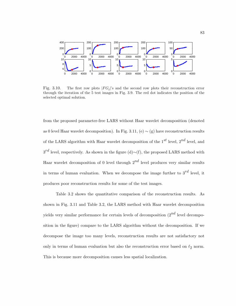
83
0 2000 40000
200
400
0 2000 4000
6
8
100 2000 4000
0
100
200
0 2000 40000
5
100 2000 4000
0
100
200
0 2000 40000
5
100 2000 4000
0
100
200
0 2000 40000
5
100 2000 4000
0
50
100
0 2000 40000
5
Fig. 3.10. The first row plots |FGi|’s and the second row plots their reconstruction errorthrough the iteration of the 5 test images in Fig. 3.9. The red dot indicates the position of theselected optimal solution.
from the proposed parameter-free LARS without Haar wavelet decomposition (denoted
as 0 level Haar wavelet decomposition). In Fig. 3.11, (e) ∼ (g) have reconstruction results
of the LARS algorithm with Haar wavelet decomposition of the 1st level, 2nd level, and
3rd level, respectively. As shown in the figure (d)∼(f), the proposed LARS method with
Haar wavelet decomposition of 0 level through 2nd level produces very similar results
in terms of human evaluation. When we decompose the image further to 3rd level, it
produces poor reconstruction results for some of the test images.
Table 3.2 shows the quantitative comparison of the reconstruction results. As
shown in Fig. 3.11 and Table 3.2, the LARS method with Haar wavelet decomposition
yields very similar performance for certain levels of decomposition (2nd level decompo-
sition in the figure) compare to the LARS algorithm without the decomposition. If we
decompose the image too many levels, reconstruction results are not satisfactory not
only in terms of human evaluation but also the reconstruction error based on ℓ2 norm.
This is because more decomposition causes less spatial localization.

84
(a)
(b)
(c)
(d)
(e)
(f)
(g)
Fig. 3.11. Image denoising results of face images. (a) Original images. (b) Occlusionoverlaid images of (a). (c) PCA reconstruction (d) LARS reconstruction without Haarwavelet decomposition. (e) ∼ (g) LARS reconstruction by applying the proposed Haarwavelet decomposition of level 1 (4 subbands, size of 32× 32), level 2 (16 subbands, sizeof 16× 16) and level 3 (64 subbands, size of 8× 8), respectively.
Reconstruction Error
(b) Occ. Imgs 5.22 7.73 8.00 3.45 10.62 10.28 15.20 8.65 13.32 9.29(c) PCA 4.60 6.63 6.92 3.23 9.07 7.31 11.14 7.12 10.90 7.73(d) LARS (level 0) 2.17 1.65 2.51 3.06 2.08 1.82 1.99 1.09 4.55 2.46(e) LARS (level 1) 2.19 1.83 2.54 2.79 2.33 2.07 1.89 1.66 4.67 2.56(f) LARS (level 2) 1.96 2.05 3.16 2.67 2.38 2.81 2.51 2.33 4.76 3.46(g) LARS (level 3) 2.22 3.24 3.59 2.50 4.68 5.36 4.29 2.97 6.03 4.95
Table 3.1. Reconstruction Error of the test images from the second row to the seventhrow of Fig. 3.11. ‖ · ‖2 represents ℓ2 norm.

85
3.6.3 Occlusion Handling for Noisy Data
In this section, we show the experimental results of noisy data cleaning by com-
paring our parameter-free LARS algorithm to Robust PCA and Local Smoothing. Ex-
periments were conducted using three image data sets: the synthetic face images used in
Section 3.6.1, a human walking video sequence (109 frames, in the size of 60× 40) and a
ballet video sequence (166 frames, in the size of 50× 45). The intensity of these images
are also normalized from 0 to 1.
For these experiments, we made a noisy test data set from each image data set by
overlaying an occlusion to a part of each image. We randomly selected approximately
30% of the images from each data set (210 images out of face data set, 33 images out of
human walking data set, and 50 images out of ballet data set) and overlaid a constant
intensity noise patch at a random location. The size of the occlusion patch is 20 × 20
pixels for the face data set, 15 × 15 pixels for the ballet data set, and 10 × 10 pixels
for the human walking data set. The intensity value of the occlusion patch is randomly
determined from 0 to 1.
To apply the LARS algorithm to the noisy data cleaning problem, we exploited
the idea of Local smoothing using WPCA [45]. For each image, we compute the local
tangent (U in Eq. 3.15) using WPCA and apply the proposed parameter-free LARS
algorithm. Fig 3.12 shows the reconstruction results of the three image data sets. In
Fig. 3.12, (a) depicts the 10 occlusion overlaid images selected from the noisy test data
set, and (b) through (d) show the reconstruction results of the LARS occlusion handling
method proposed in this paper, the Local Smoothing algorithm proposed in [45], and

86
Robust PCA proposed in [15], respectively. For the results of (c) and (d), we ran the
algorithms several times by varying the parameters which the algorithms need, and the
best results were selected by considering the reconstruction error based on the ℓ2 norm
and visual evaluation.
Table 3.2 shows the quantitative results of the reconstruction error based on ℓ2
norm. It contains the average and the standard deviation of the reconstruction errors
for each test data set obtained by applying the three occlusion handling algorithms.
The column of “Only Occ.” contains the reconstruction error computed only using the
30% of the occlusion overlaid images from each test data set, and the column of “All”
contains the reconstruction error computed using all of the images in each test data
set. It is inevitable that non-occlusion images are degraded while the occlusion handling
algorithms deal with the occlusion images. We separate the error into “Only Occ.” and
“All” in order to measure how the algorithms perform not only for the occlusion images
but also for all the images. In most cases, the proposed LARS algorithm and Local
Smoothing algorithm preserve the non-occlusion images very well.
As shown in Fig. 3.12 and Table 3.2, the proposed LARS algorithm performs
better than the other two methods in terms of visual evaluation as well as ℓ2 based
quantitative reconstruction error. Our algorithm outperformed the others especially for
complicated texture images such as face images.
We also conducted experiments using the video data set used in [15]. The video
data set contains 506 images of size of 160×120 pixels, which captured an outdoor scene
for two days. Some of the images include humans in the scene, which are considered
as outliers, while the majority of the images contains only the outdoor background. In

87
LARS Local Smoothing RPCA
Only Occ. All Only Occ. All Only Occ. AllFace 3.17 (1.71) 2.86 (1.33) 4.70 (1.79) 3.72 (1.62) 6.77 (2.50) 5.14 (1.85)Ballet 3.11 (1.31) 2.54 (1.01) 3.76 (1.20) 3.29 (1.13) 4.70 (1.16) 4.49 (1.04)
Walking 3.31 (0.76) 2.95 (0.72) 4.39 (0.86) 3.86 (0.82) 3.75 (1.09) 3.68 (0.92)
Table 3.2. Average reconstruction errors based on ℓ2 norm and their standard deviation (insidethe parenthesis).
these experiments, we compared the experimental results between the RPCA algorithm
and the proposed LARS occlusion handling method with local smoothing. For the LARS
algorithm, we decompose each image into 64 subbands of size 15× 20 pixels by applying
3rd level Haar wavelet decomposition. As shown in Fig. 3.13, both of the methods
perform similarly for the video images based on human evaluation. It is not easy to
provide quantitative comparison between two algorithms because no prototype data set
is provided for the computation of the quantitative error.
In general, RPCA loses much of the original detail of the images, which is why
RPCA performed poorly in the first three experiments. RPCA was able to perform
adequately with the outdoor video set, primarily because in an outdoor scene, the main-
tenance of detail is not very important. The proposed LARS algorithm performed well in
all four experiements, while maintaining a high level of the detail of the original images.
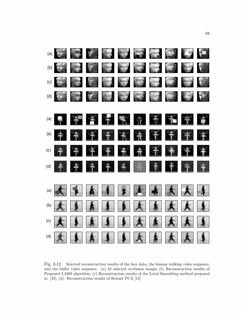
88
(a)
(b)
(c)
(d)
(a)
(b)
(c)
(d)
(a)
(b)
(c)
(d)
Fig. 3.12. Selected reconstruction results of the face data, the human walking video sequence,and the ballet video sequence. (a) 10 selected occlusion images (b) Reconstruction results ofProposed LARS algorithm, (c) Reconstruction results of the Local Smoothing method proposedin [45], (d): Reconstruction results of Robust PCA [15]

89
(a)
(b)
(c)
(d)
(e)
Fig. 3.13. (a) 20 selected occlusion overlaid images from video sequence. (b) LARSreconstruction. (c) Absolute images between (a) and (b). (d) RPCA reconstruction. (e)Absolute images between (a) and (d).

90
Chapter 4
Spectral Clustering for Robust Motion Segmentation
In this chapter, we deal with the issues related to the matrix factorization meth-
ods for motion segmentation. We first show that the shape interaction matrix can be
extracted from the trajectory matrix using QR decomposition with pivoting, an idea
that was briefly mentioned in [14]. As a by-product we give a simple and clean proof
of the subspace separation theorem described in [31]. We then observe that the shape
interaction matrix is very similar to the weight matrix used for graph partitioning and
clustering [55] [23] [17] [67], and the motion segmentation problem can be cast as an
optimal graph partitioning problem. To this end, we apply the spectral k-way clustering
method [23] [17] to the shape interaction matrix to transform it into near-block diagonal
form. In our particular application, we use QR decomposition based technique for clus-
ter assignment. This technique at the same time also provides confidence levels of the
cluster membership for each feature point trajectory. This confidence levels provide a
more robust cluster assignment strategy. We assign a feature point directly to a cluster
when it has a high confidence level for the cluster compared to those for other clusters.
Using the assigned feature points in each cluster, we compute a linear subspace in the
trajectory space. Because the other feature points have lower confidence levels, their
cluster memberships are determined by their distances to each of the linear subspaces.

91
Our experiments on both synthetic data sets and real video images have shown that this
method is very reliable for motion segmentation even in the presence of severe noise.
4.1 Matrix Factorization Method for Shape Recovery and Motion Seg-
mentation
Tomasi and Kanade [61] first introduced a factorization method which has been
widely used in shape recovery and motion segmentation. In this method, given a video
sequence, a group ofN feature points are tracked along the F frames. The 2D coordinates
are stacked by yielding a matrix, P , whose row corresponds the coordinates of each frame
and whose column corresponds to those of each feature point.
Suppose that we are given a set of N feature points tracked through F frames, we
can construct a feature trajectory matrix P ∈ R2F×N where the rows correspond to the
x or y coordinates of the feature points in the image plane and the columns correspond
to the individual feature points. The factorization method decomposes the matrix, P ,
into two matrices which, respectively, represent camera motion, M , and object shape,
S. Eq. 4.1 shows this factorization. The method deals with a single static object viewed
by a moving camera.

92
P = MS (4.1)
u11 · · · u1N
......
...
uF1 · · · uFN
v11 · · · v1N
......
...
vF1 · · · vFN
=
iT1| tx1
... | ...
iTF| txF
jT1| ty1
... | ...
jTF| tyF
[s1, · · · , sN ] (4.2)
where (ufi, vfi) are the feature image position, vectors iTf
= [ix, iy, iz ], jTf
=
[jx, jy, jz ] are the first two rows of the rotation matrix at instant f , and (txf , tyf ) are
the X and Y coordinates of the position of the object’s coordinate frame, in the camera
frame, at the same instant. The rank of matrix P is at most 4 because the ranks of M
and S are at most 4. If we decompose the matrix P using Singular Value Decomposition
(SVD) by taking only the 4 biggest singular values and their corresponding eigen vectors,
we can compute the matrix M and S.
P = UΣV T = (UΣ1/2)(Σ1/2V T ) = (UΣ1/2A)(A−1Σ1/2V T ) = MS (4.3)
where, A is a nonsingular 4x4 matrix.

93
Costerira and Kanade [14] extended and expanded the above method to account
for multiple objects moving independently in a sequence of images. To achieve this, they
introduced the shape interaction matrix, Q = VVT , where V is obtained from UΣV T
(the SVD of P ). It is invariant to both the object motions and the selection of coordinate
systems. It is assumed that the matrix P has N feature points tracked from K objects
and the feature points of each object are grouped together ,i.e. P = {P1, · · · , PK}. As
discussed in [14], the shape interaction matrix has a block diagonal form as follows:
Q = VVT = diag{ST1
Λ1S1, · · · , STK
ΛKSK} (4.4)
where Si is a shape matrix of object i and Λi is 4x4 matrix of the moments of inertia of
object i. Unless the matrix P is a canonical form (which it rarely is), rows and columns
of Q are iteratively permuted in such a way that the feature points of the same object
are arranged adjacently into blocks, transforming Q into the canonical shape interaction
matrix Q. However, Q is very sensitive to noise. If P has noise, then the Q will not have
a clear block diagonal form.
To overcome this weakness, several methods have been proposed. Below, we
highlight some of the more prominent methods.
Gear[21] exploited the reduced row echelon form of the shape interaction matrix
to group the points to the linearly independent subspace. If there is no errors, any two
columns of the echelon form which have nonzero elements in the same row correspond
to points belonging to the same rigid body. The echelon form matrix is represented by
a weighted bipartite graph and uses a statistical approach to estimate the grouping of

94
points to subspaces in the presence of noise by computing which partition of the graph
has the maximum likelihood.
Ichimura [28] suggested a motion segmentation method based on discriminant
criterion [44] features. The main idea of this method is to select useful features for
grouping noisy data. Using a noise-contaminated shape interaction matrix, it computes
discriminant criterion for each row of the matrix. The feature points are then divided into
two groups by the maximum discriminant criterion, and the corresponding row gives the
best discriminant feature. The same procedure is applied recursively to the remaining
features to extract other groups.
Wu et. al. [64] proposed an orthogonal subspace decomposition method to deal
with the noisy problem of the shape interaction matrix. This method decomposes the
object shape space into signal subspaces and noise subspaces. They then use the shape
signal subspace distance matrix, D, for shape space grouping. This procedure is sum-
marized as follows. First, points are clustered into group fragments using the shape
interaction matrix Q by applying simple thresholding or discriminant analysis method
described in [28]. Second, the signal subspace projection matrix is calculated for each
fragment by applying SVD, which is used to compute the distance matrix D. Third,
the group fragments are merged into an independent object based on D. Finally, the
motion and structure for each object are computed based on segmentation.
Kanatani [31] [32] reformulated the motion segmentation problems based on the
idea of subspace separation. This approach divides the given N feature points to form
m disjoint subspaces Ii, i = 1, · · · ,m. Provided that the subspaces are linearly in-
dependent, the elements Qij in the shape interaction matrix Q are zero if the point i

95
and the point j belong to different subspaces. Kanatani also pointed out that even a
small amount of noise in one feature point can affect all the elements of Q in a compli-
cated manner. Based on this, Kanatani proposed noise compensation methods using the
original matrix W rather than the shape interaction matrix Q.
Zelnik-Manor and Irani [66] showed that different 3D motions can also be captured
as a single object using previous methods when there is a partial dependency between the
objects. They suggested using an affinity matrix Q where Qij =∑
k exp(vk(i)− vk(j))2,
where vk’s are the largest eigenvectors of Q. They also dealt with the multi-sequence
factorization problems for temporal synchronization using multiple video sequences of
the same dynamic scene.
4.2 Multibody Motion Segmentation Algorithms
Extending the factorization method discussed in Section 4.1, Costerira and Kanade [14]
proposed a multibody factorization method which separates and recovers the shape and
motion of multiple independently moving objects in a sequence of images. To achieve
this, they introduce a shape interaction matrix which is invariant to both the object mo-
tions and the selection of coordinate systems, and suggest a greedy algorithm to permute
the shape interaction matrix into block diagonal form. Gear [21] exploited the reduced
row echelon form of the shape interaction matrix to group the feature points into the lin-
early independent subspaces. For Gear’s method, in the noise-free case, any two columns
of the echelon form which have nonzero elements in the same row correspond to feature
points belonging to the same rigid body. The echelon form matrix can be represented
by a weighted bipartite graph. Gear also used a statistical approach to estimate the

96
grouping of feature points into subspaces in the presence of noise by computing which
partition of the graph has the maximum likelihood.
Ichimura [28] suggested a motion segmentation method based on discriminant
criterion [44] features. The main idea of the method is to select useful features for
grouping noisy data. Using the noise-contaminated shape interaction matrix, it computes
discriminant criterion for each row of the matrix. The feature points are then divided
into two groups by the maximum discriminant criterion, and the corresponding row
gives the best discriminant feature. The same procedure is applied recursively to the
remaining features to extract other groups. Wu et. al. [64] proposed an orthogonal
subspace decomposition method to deal with the noisy problem of the shape interaction
matrix. The method decomposes the object shape space into signal subspaces and noise
subspaces. They used the shape signal subspace distance matrix, D, for shape space
grouping rather than the noise-contaminated shape interaction matrix.
Kanatani [31] [32] reformulated the motion segmentation problems based on the
idea of subspace separation. The approach is to divide the given N feature points to
form m disjoint subspaces Ii, i = 1, · · · ,m. A rather elaborated proof was given showing
that provided that the subspaces are linearly independent, the elements Qij in the shape
interaction matrix Q is zero if the point i and the point j belong to different subspaces.
Kanatani also pointed out that even a small noise in one feature point can affect all the
elements of Q in a complicated manner. Based on this fact, Kanatani proposed noise
compensation methods using the original data rather than the shape interaction matrix
Q.

97
Zelnik-Manor and Irani [66] showed that different 3D motions can also be captured
as a single object using previous methods when there is a partial dependency between
the objects. To solve the problem, they suggested to use an affinity matrix Q where
Qij =∑
k exp(vk(i)− vk(j))2, where vk’s are the largest eigenvectors of Q. They also
dealt with the multi-sequence factorization problems for temporal synchronization using
multiple video sequences of the same dynamic scene.
4.3 Constructing the Shape Interaction Matrix Using QR Decomposi-
tion
In this section, we exhibit the block diagonal form of the shape interaction matrix
using QR decomposition with pivoting [22]. Assumimg that we have N rigidly moving
feature points, p1, . . . , pN , which are on an image plane which corresponds 3D points
over the F frames. Motion segmentation can be interpreted as dividing the feature points
pi into S groups [31] each spanning a linear subspace corresponding to feature points
belonging to the same object. We denote the grouping as follows,
{1, . . . , N} =S⋃
i=1
Ii, Ii ∩ Ij = ∅.
Now define li = |Ii| which is the number of the points in the set Ii, and ki=dim
span{pj}j∈Ii≤ li and Pi = {pj}j∈Ii .
Let the SVD of Pi be Pi = UiΣiVti, where Σi ∈ Rki×ki , i = 1, . . . , S. Then
P = [P1, P2, . . . , Ps] can be written as,

98
P = [P1, P2, . . . , Ps] = [U1Σ1, U2Σ2, . . . , UsΣs]
V T1
0 · · · 0
0 V T2· · · 0
......
. . ....
0 0 · · · V Ts
, (4.5)
where rank(Vi)=ki for i = 1, · · · , s. Assuming that the S subspaces span{pj}j∈Ii, i =
1, . . . , S are linearly independent, then the matrix [U1Σ1, U2Σ2, . . . , UsΣs] has a full
column rank of k = k1 + · · · + ks. Therefore, an arbitrary orthonormal basis for the
row space of P can be written as Φdiag(V1, · · · , Vs)T for an arbitrary orthogonal matrix
Φ ∈ Rk×k. Now the shape interaction matrix can be written as
Q = diag(V1, · · · , Vs)ΦTΦdiag(V1, · · · , Vs)
T = diag(V1VT1, · · · , VsV
Ts
).
This clearly shows that Qij = 0 if i and j belong to different subspaces, i.e., if the
corresponding feature points belong to different objects.
Rather than using SVD, a cheaper way to compute an orthonormal basis for the
row-space of P is to apply QR decomposition with column pivoting to PT ,
PTE = QR, (4.6)
where E is a permutation matrix, and Q has k columns. It is easy to see that
QQT = Q. In the presence of noise, P will not exactly have the rank k, but generally

99
QR decomposition with column pivoting generates a R matrix that reliably reveals the
numerical rank of P. We can then truncate R by deleting rows with small entries.
4.4 Motion Segmentation
4.4.1 Spectral Multi-way clustering
In the last section, we showed that the shape interaction matrix, Q ∈ RN×N has
a block diagonal form when the feature points are grouped into independent subspaces
corresponding to S different objects. In general, this grouping is unknown, and we need
to find row and column permutations of the matrix Q to exhibit this block diagonal
form, and thus assigning the feature points to different objects. A greedy algorithm has
been proposed in [14] but it performs poorly in the presence of noise. We now present a
more robust method based on spectral graph clustering [55] [23] [17] [67]. It provides a
confidence level from which we can further refine the cluster memberships of the feature
points.
The absolute value of the (i, j) element of the shape interaction matrix Q measures
the similarity of feature points i and j. Feature points belonging to the same object will
have a high degree of similarity whereas feature points belonging to different object will
have a low degree of similarity. In fact, in the noise-free case, feature points in different
objects will have zero similarity. Our goal is then to partition the feature points into S
groups based on similarity. Let W = (wij) with wij = |Qij |. For a given partition of
the feature points into S groups, we can permute the rows and columns of W so that
the rows and columns corresponding to the feature points belonging to the same objects

100
are adjacent to each other, i.e., we can re-order the columns and rows of the W matrix
such that
W =
W11 W12 · · · W1S
W21 W22 · · · W2S
· · · · · · ...
WS1 WS2 · · · WSS
. (4.7)
We want to find a partition such that Wii will be large while Wij , i 6= j will be small,
and to measure the size of a sub-matrix matrix Wij we use the sum of all its elements
and denoted as sum(Wij). Let xi be a cluster indication vector accordingly partitioned
with that of W with all elements equal to zero except those corresponding to rows of
Wii,
xi = [0 · · · 0, 1 · · · 1, 0 · · · 0]T .
Denote D = diag(D1, D2, · · · , DS) such that Di =∑Sj=1
Wij . It is easy to see that
sum(Wii) = xTiWxi,
∑
j 6=isum(Wij) = xT
i(D −W )xi.
Since we want to find a partition which will maximize sum(Wii) while minimizing
sum(Wij), i 6= j, we seek to minimize the following objective function by finding a set of
indicator vectors xi. The objective function is called min-max cut in [23] [17] which is
a generalization of the normalized cut objective function [55] to the multi-way partition
case.

101
MCut =xT1
(D −W )x1
xT1Wx1
+xT2
(D −W )x2
xT2Wx2
+ · · ·+xTS
(D −W )xS
xTSWxS
=xT1Dx1
xT1Wx1
+xT2Dx2
xT2Wx2
+ · · ·+xTSDxS
xTSWxS
− S.
If we define yi = D1/2xi/||D1/2xi||2 and YS = [y1, · · · , yS ], we have
MCut =1
yT1Wy1
+1
yT2Wy2
+ · · ·+ 1
yTSWyS
− S (4.8)
where W = D−1/2WD−1/2 and yi =D1/2xi
‖D1/2xi‖2. It is easy to see that each vector
yi is orthogonal to all the other vectors and is normalized to have Euclidean norm
one. If we insist that each vector yi be constrained to inherit the discrete structure
of its corresponding indicator vector xi, we then solve the combinatorial optimization
problem which has been proven to be NP-hard even when S = 2 [55]. The idea of
spectral clustering instead is to relax these constraints and allow each vector yi to be
an arbitrary set of orthonormal vectors. In this case, the minimum of Eq. 4.8 can be
achieved by orthonormal basis y1, · · · , yS of the subspace spanned by the eigenvectors
corresponding to the largest S eigenvalues of W . Next we discuss how to assign the
feature points to each cluster based on the eigenvectors.
At this point, we should mention that the cluster assignment problem in spectral
clustering is not well-understood. Here we follow the approach proposed in [67]. As-
suming Y = [y1, · · · , yS ]T denotes the optimal solution of Eq. 4.8, the vectors yi can

102
be used for cluster assignment because yi ≈ D1/2xi/||D1/2xi||2, where xi is the cluster
indicator vector of i − th cluster. Ideally, if W is partitioned perfectly into S clusters,
then the columns in X = [xi, · · · , xS ]T of the i − th cluster are the same, one for the
i− th row and zeros for the others. Two columns of different clusters are orthogonal to
each other. Because of this, Y approximately inherits this property: two columns from
two different clusters are orthogonal to each other, and those from one cluster are the
same. We now pick a column of Y which has the largest norm yi and orthogonalize the
rest of the columns of Y against this column. We then assign the columns to cluster
i whose residual is small. We perform this process S times. As discussed in [67], it is
exactly the same procedure of QR decomposition with column pivoting applied to Y .
In particular, we compute the QR decomposition of Y T with column pivoting
Y TE = QR = Q[R11, R12]
where Q is a S × S orthogonal matrix, R11 is a S × S upper triangular matrix, and E
is a permutation matrix. Then we compute the matrix R as
R = R−111
[R11, R12]PT = [IS , R−111R12],
The matrix R ∈ RS×N gives the confidence level of each point to be assigned
to each cluster. Notice that the columns correspond to the feature points and the rows
correspond to the clusters. The cluster membership of each feature point is determined
by the row index of the largest element (based on the absolute value of the corresponding

103
column of R). This provides us with a baseline for motion segmentation which accounts
for the presence of noise.
This presents a problem however. Although we can assign a point to a cluster
with high confidence when there is a very dominantly high confidence value in the corre-
sponding column, we can not assign a point to a cluster with high confidence when two
or more values in a column are very close to each other. Table 4.4.1 shows an example
of the matrix R ∈ R3×10 that has 10 points extracted from 3 objects. The last row of
the table shows the cluster membership of each point assigned by the row index of the
highest absolute value. For instance, the point p1 is assigned to cluster 2 because the
second row value (0.329), is greater than the other row values (0.316 and 0.203). How-
ever, we cannot have much confidence of its membership because there is no dominant
value in the corresponding column.
Although this is a problem, we do have a baseline for motion segmentation which
accounts for the presence of noise. Further improvement can be achieved as we discuss
next.
Cluster ID p1 p2 p3 p4 p5 p6 p7 p8 p9 p10k = 1 0.32 0.35 0.88 0.33 0.46 0.56 0.09 0.28 0.07 0.12k = 2 0.33 0.34 0.03 0.37 0.01 0.06 0.19 0.71 0.82 0.83k = 3 0.20 0.02 0.03 0.17 0.57 0.56 0.78 0.13 0.09 0.11
Assigned Cluster 2 1 1 2 3 1 3 2 2 2
Table 4.1. An example of the matrix R. There are 10 points extracted from 3 objects.The last row shows the assigned cluster

104
4.4.2 Refinement of cluster assignment for motion segmentation
Baseline spectral clustering shows its robustness for a noisy environment in spite
of its hard clustering (assigning each point to a cluster even though it does not have
high confidence for it). This method alone, however, can sometimes fail in presence of
severe noise. In this section, we discuss a two-phase approach whereby in phase one we
assign the cluster memberships for those feature points with high confidence levels, and
in phase two we construct linear subspaces for each cluster based on the high confidence
feature points, and assign the rest of the feature points by projecting them onto these
subspaces.
Our approach proceeds as follows. After computing R discussed in the previ-
ous section, the points of high confidence for each clusters are selected. Let’s define
Pi = [pi1, · · · , piNi] as the trajectory points in the cluster i. One of the easiest methods
is applying a threshold to the values of each column. If the highest value in the column
is greater than the threshold, the point is assigned to the corresponding cluster. Other-
wise, the point is assigned to cluster 0 which is in a pending state to decide its cluster
membership. Referring to the pending points as P0 = [p01, · · · , p0N0], the next step
is to compute subspace(2D) for pi1, · · · , piNi, i = 1, · · · , S using Principal Component
Analysis (PCA). Thus, with Ui denoting a subspace basis for the cluster i, we finally
determine the cluster membership of each pending point by computing the minimum
distance from the point to the subspaces.
θj = argmini||p0j − (ci + UiU
Ti
(p0j − ci))||2,

105
(a)
(b)
Fig. 4.1. The two synthetic video sequences used in [32] and [33] respectively. (a). 20green dots are background pixels and 9 foreground points (b). 24 background points and14 foreground points. The foreground pixels are connected with lines.
where j = 1, · · · , S and ci =∑Nij=1 pij .
The point p0j is assigned to the cluster θj .
4.5 Experimental Results
4.5.1 Synthetic Data
Fig. 4.1 shows two synthetic image sequences used for performance evaluation.
Actually these images are used in [32] and [33]. Fig. 4.1-(a), denoted as Synthetic 1, has
20 background points(green dots) and 9 foreground points(red dots). Fig. 4.1-(b),denoted
as Synthetic 2, has 24 background points and 14 foreground points. The foreground
points are connected by lines for visualization purpose.
We performed experiments using not only the original tracking data but also the
data added by independent Gaussian noise of mean 0 and standard deviation σ to the

106
coordinates of all the points. For the noise data, we generated 5 sets for each σ = 1, 2, 3, 4,
and computed the misclassification rate by simply averaging the 5 experiment results.
We compared the two methods proposed in this paper (One is k-way Min-Max cut
clustering in Section 4.4.1 denoted as Method 1, and the other is a combination of the
k-way Min-Max cut clustering and clustering refinement using subspace projection in
Section 4.4.2 denoted as Method 2) to the Multi-stage optimization proposed in [33]
denoted as Multi-Stage. Table 4.2 shows that the misclassification rates of the three
methods over the different noise levels (σ = 0, 1, 2, 3, 4). Method 2 and Multi-Stage
performed better than Method 1. In fact, these two methods were almost perfect for
the sequences.
Video Seq. noise σ = 0 σ = 1 σ = 2 σ = 3 σ = 4Method 1 0.0 1.4 1.4 0.7 0.7
Synthetic 1 Method 2 0.0 0.0 0.0 0.0 0.0Multi-Stage 0.0 0.0 0.7 0.0 0.0
Method 1 8.2 10.6(1.6) 11.7(2.1) 11.7(3.6) 13.2(1.7)Synthetic 2 Method 2 0.0 0.0 0.0 0.0 0.59(1.3)
Multi-Stage 0.0 0.0 0.0 0.0 0.59(1.3)
Table 4.2. Misclassification rate (%) for the two synthetic sequences. The values inparentheses are the standard deviation values. Method 1 is the k-way Min-Max cutclustering discussed in Section 4.4.1 and Method 2 is the k-way Min-Max cut cluster-ing plus the clustering refinement using subspace projection discussed in Section 4.4.2.Multi-Stage is the Multi-stage optimization proposed in [33].

107
4.5.2 Real Video Sequences
We experimented with the real video sequences used in [33]. In all these sequences,
both the foreground object and the background are simultaneously moving because the
camera is moving. The video sequences are denoted as video1, video2 and video3 respec-
tively. In addition, by overlaying the foreground feature points in video1 to video2, we
synthesized a fourth test video sequence which has 2 moving objects and a background
denoted as video4. Fig. 4.2 shows 5 selected frames for each of the four sequences.
We also performed experiments using not only the original tracking data but
also the data added by independent Gaussian noise of mean 0 and standard deviation
σ to the coordinates of all the points. For the noise data, we generated 5 sets for
each σ = 3, 5, 7, 10, and computed the misclassification rate by simply averaging the 5
experiment results.
Table 4.3 shows the misclassification rates of the three methods over the different
noise levels (σ = 0, 3, 5, 7, 10). Method 1 performs very well for a noise-free environ-
ment as predicted. However, with noisy environment, this method performs poorly as
it misclassifies some points. Multi-Stage performs very well for video1 through video3
even in the presence of noise. However, it performs poorly for video4 possibly because of
the presence of two moving objects. Based on our experiments, this method also suffers
from the local minima problem. That is, using the same data, it yields different results
based on the initialization. That is the reason the standard deviation for the method is
so high shown in Table 4.3.

108
Method 2 performs well for all four video sequences, even with multiple objects
and severe noise.
Video Seq. noise σ = 0 σ = 3 σ = 5 σ = 7 σ = 10Method 1 0.0 0.0 0.0 0.0 0.0
video1 Method 2 0.0 0.0 0.0 0.0 0.0Multi-Stage 0.0 0.0 0.0 0.0 0.0
Method 1 0 1.6(1.2) 1.6(1.2) 1.6(1.2) 2.9(1.7)video2 Method 2 0.0 0.0 0.0 0.0 0.0
Multi-Stage 0.0 0.0 0.0 0.0 7.3(16.3)
Method 1 0.0 2.5(0.01) 2.5 1.3 2.5video3 Method 2 0.0 0.0 0.0 0.0 0.0
Multi-Stage 0.0 0.0 0.0 0.0 0.0
Method1 0.0 0.7(1.6) 3.4(4.7) 8.3(5.0) 9.6(6.5)video4 Method2 0.0 0.0 0.0 0.0 0.7(1.6)
Multi-Stage 0.0 4.1(9.3) 8.2(9.6) 16.2 (13.2) 19.23 (9.87)
Table 4.3. Misclassification rate (%) for the real video sequences. The values in paren-theses are the standard deviation values.

109
Fig. 4.2. Real video sequences with the feature points. 1st row: video1, 2nd row: video2,
3rd row: video3, 4th row: video4 (foreground feature points in video1 are overlaid ontovideo2). Red dots correspond to the background while green dots correspond to theforeground. The yellow cross marks in video4 represent the foreground feature points ofvideo1
0 2 4 6 8 10−5
0
5
10
15
20
25
30
Standard Deviation
Method 1Method 2Multi−Stage
(%)
0 2 4 6 8 10−5
0
5
10
15
20
25
30
Standard Deviation
Method 1Method 2Multi−Stage
(%)
0 2 4 6 8 10−5
0
5
10
15
20
25
30
Standard Deviation
Method 1Method 2Multi−Stage
(%)
(a) video2 (b) video3 (c) video4
Fig. 4.3. Graph for misclassification rate. Graph of video1 is not depicted here becauseall of the methods perform perfectly. Method 1: Dashed-dot blue line, Method 2:Red line and Multi-Stage: Dashed green line

110
Chapter 5
Summary and Conclusions
Chapter 2 focused on outlier handling and noise reduction for a set of noisy sample
points using local linear smoothing. We showed that the local smoothing method is very
effective not only in reducing Gaussian noise but also for effective handling of outliers.
The performance of this method, however, depends on two parameters: the number of
neighbors k used in local smoothing and the γ used for weight computation. As far as
γ is concerned, experiments show that relatively low values for γ yield good results for
the case when most points in the data are corrupted by Gaussian noise. If many points
are involved in a manifold and some outliers are added to the data, a relatively high
γ tends to produce better results. For choosing the parameter k, the neighbor points
selected should approximately form a linear affine subspace. However, the results are
relatively insensitive to the choice of k as is shown in Fig. 2.6. The experiments using
the image data sets also show that the proposed local smoothing method has a potential
to remove occlusions overlaid on images. We further show that the proposed methods
can be utilized with various manifold learning methods as a preprocessing procedure to
obtain a more accurate reconstruction of the underlying nonlinear manifolds.
In Chapter 3, we proposed a parameter-free image denoising method using the
LARS algorithm, local WPCA and a statistical model selection criterion along with a

111
thresholding technique. The method adapts the ℓ1 penalized optimization method pro-
posed in [63] which identifies and updates only the noise corrupted pixels simultaneously.
The method proposed in [63], however, requires a parameter to control the size of the
pixels to be updated. We implemented the image denoising method without the param-
eter by converting the problem into a LARS problem and solving it using the LARS
algorithm. The LARS algorithm yields a family of solutions covering one updated pixel
to all of the updated pixels. Among the solutions, we determined the final optimal so-
lution utilizing a thresholding algorithm and AIC. The experimental results show that
the proposed method performs quite well in the most cases by selecting a solution in the
vicinity of the global minimum of reconstruction error without a parameter to controls
the number of pixels to be updated.
We also proposed a method for decomposing an image into several independent
subbands (blocks) of the same size, by slightly modifying the original Haar wavelet anal-
ysis. It is possible to decrease the time complexity by applying each subband to the
algorithm independently. The method, however, might lose the spatial localization (low
resolution) as the decomposition level gets deeper and deeper. The proposed image de-
composition method provides relatively similar results for certain levels of decomposition
without losing too much spatial resolution. If the decomposition level is too deep, we lose
of too much spatial details and obtain poor reconstruction results. The proposed decom-
position method is suitable for parallel computing because the subbands are independent
of each other as proven in Section 3.5.
We utilized the occlusion handling algorithm as a preprocessing tool for cleaning
training data, which contain occlusion overlaid images, for an automatic learning system.

112
The experimental results show that the proposed method is very promising for this
purpose.
In chapter 4, we proposed a robust motion segmentation method using matrix
factorization, subspace separation and spectral graph partitioning. First, we mathemat-
ically proved that the shape interaction matrix can be computed using QR decomposition
which is more effective than SVD. We solved the motion segmentation problem using
the spectral graph clustering technique because the shape interaction matrix has a very
similar form to the weight matrix of the graph. We apply the Spectral Relaxation K-way
Min-Max cut clustering method [23] [17] to the shape interaction matrix. It provides a
relaxed cluster indication matrix. QR decomposition was then applied to the matrix,
which generated a new cluster indication matrix, to determine the cluster membership
of each point. The values of the new cluster indication matrix reflect a confidence level
for each point to be assigned to clusters. This method yields a good performance in a
noise free environment, but it is sensitive to noise. We proposed a robust motion seg-
mentation method by combining the spectral graph clustering and subspace separation
to compensate for the noise problem. Initially, we assigned only points of high confidence
to clusters based on the cluster indication matrix. We computed the subspace for each
cluster using the assigned points. We finally determined the membership of the other
points, which are not assigned to a cluster, by computing the minimum residual when
they are projected to the subspace.
We used the two synthetic image sequences and three real video sequences from [33]
and a generated a fourth real video sequence, all of which were overlaid with various sever-
ity of noise. The proposed method performed almost to perfection with the synthetic

113
image sequences, and performed very well with the real video sequences even with severe
noise and with multiple objects. In comparison, although the Multi-Stage optimization
method [33] performed reasonably well with both synthetic and real video sequences,
it performed very poorly in the presence of multiple objects and suffers from the local
minima problem.
5.0.3 Contributions
We proposed a robust outlier handling and noise reduction method that can be
used in conjuction with nonlinear manifold learning methods as a preprocessing proce-
dure to obtain a more accurate reconstruction of the underlying nonlinear manifold. A
closed-form solution of Weighted PCA (WPCA), which is discussed in Section 2.2, is
proposed for the method by only considering object-level outliers. With both object-
level and feature-level outliers, WPCA solves the optimization problem in an iterative
fashion, see [15] for example. We successfully applied the local smoothing method to the
image occlusion handling problem and point-based rendering problem, and showed the
robustness of this method.
We also proposed a robust parameter-free image occlusion handling algorithm.
The main contributions of this research include: 1) We showed that the the image denois-
ing problem can be solved using the LARS algorithm; 2) We proposed a parameter-free
approach to image denoising utilizing a thresholding technique and the statistical model
selection criterion of AIC; 3) We demonstated how sub-block decomposition affect com-
putation time; and 4) We showed that the proposed LARS algorithm can be successfully

114
used as a preprocessing tool for cleaning noisy data which contains occlusion overlaid
images.
In Chapter 4, we proposed a robust motion segmentation method using matrix
factorization, subspace separation and spectral graph partitioning. We showed that the
shape interaction matrix can be computed using QR decomposition instead of Singular
Value Decomposition (SVD), where QR decomposition is more stable and efficient than
SVD. A spectral graph clustering technique is applied to the shape interaction matrix
for the final grouping of the feature points into independent objects.
5.0.4 Future Works
Several issues deserve further investigation. First, there are three issues for local
smoothing for manifold learning in Chapter 2: 1) automatic selection of parameters such
as the number of neighbors and γ for weight computation; 2) exploiting RPCA [15] for
image data which assigns weights to the pixels and/or images; and 3) exploiting different
metrics such as tangential distance to compute k nearest neighbors for image data sets
rather than the Euclidean distance.
The LARS algorithm still requires a high computation time because the size of
matrix X in Eq. 3.12 is very large (the number of pixels × the number of pixels), com-
puting the solutions one pixel at a time. If we compute the solutions several pixels at a
time, we can reduce the computation time significantly. We also used Euclidean distance
to compute the nearest neighbors for each local tangent. It is possible to exploit dif-
ferent metrics such as Kullback-Leibler distance, tangential distance, etc. Sophisticated
thresholding algorithms can also be used for optimal solution estimation.

115
For motion segmentation using matrix factorization as discussed in Chapter 4,
finding a proper rank for SVD in matrix factorization is very critical for performance.
Automatic estimation of the rank of SVD should be studied further. Current multi-body
motion segmentation algorithms using matrix factorization deal with rigid objects. It
is plausible if we can also deal with motion segmentation of articulate objects. Because
the shape of each object is constantly changing, a fundamental question is raised: What
is the definition of an independently moving object? Once a definition is established, we
can then begin to address the problems associated with motion segmentation of articulate
objects, and it would be considered breakthrough work for a multitude of motion related
areas, such as real-life human motion analysis and the like.

116
Appendix A
Computation of the Equiangular vector uA, w and AA
uA is defined as the unit vector with equal angles, less than 90◦, with the columns
of XA. Therefore, we can obtain the following facts. uA can be expressed by a linear
combination of the columns of XA, and all the inner products between uA and the
columns of XA should be the same.
uTAuA = 1 (A.1)
uA = XAw (A.2)
XTAuA = AA1A (A.3)
where AA is cosine value between uA and the columns of XA.
From this, we obtain Eq. A.4 by applying Eq. A.2 to Eq. A.1.
wTXTAXAw = 1 (A.4)
We obtain w by substitute XAw in Eq. A.2 for u in Eq. A.3 as shown in Eq. A.5
.

117
XTAXAw = AA1A
w = (XTAXA)−1AA1A = G−1
A AA1A (A.5)
From here, we apply Eq. A.5 to Eq. A.4, deriving Eq. A.6.
A2A1TA(XT
AXA)−11A = 1
We only need positive AA because we allow the angle between uA and each
column of XA to be less than 90◦. Therefore, we can obtain AA.
AA = (1TA(XTAXA)−11A)−
12 = (1TAG
−11A)−12 (A.6)

118
Appendix B
2D Haar Wavelet Analysis
φ(x, y) =
1 if 0 ≤ x < 1 and 0 ≤ y < 1
0 otherwise
(B.1)
φ(x, y) = φ(x)φ(y) (B.2)
Suppose a function fj(x, y),
fj(x, y) =∑
k1∈Z
∑
k2∈Zajk1,k2
φ(2jx− k1, 2jy − k2).
Then fj(x, y) can be decomposed into x and y components as shown in Eq. B.3.
fj(x, y) =∑
k1∈Z
∑
k2∈Zajk1,k2
φ(2jx− k1)φ(2jy − k2) (B.3)
=∑
k1∈Zajk1φ(2jx− k1)
∑
k2∈Zajk2φ(2jy − k2)
Next, we use Eq. 3.38, we obtain,

119
fj(x, y) = (wxj−1
+ fxj−1
)(wxj−1
+ fxj−1
) (B.4)
= wxj−1
wyj−1
+ wxj−1
fyj−1
+ fxj−1
wyj−1
+ fj−1(x, y), (B.5)
where the superposition character x and y mean the direction of 1D Haar wavelet
analysis.

120
References
[1] H. Akaike. Information theory and an extension of the maximum likelihood princi-
ple. In 2nd International Symposium on Information theory, pages 267–281, 1973.
[2] H. Akaike. A new look at the statistical model identification. IEEE Transactions
on Automatic Control, 19:716–723, 1974.
[3] H. Akaike. A bayesian analysis of the minimum aic procedure. Annals of the Institute
of Statistical Mathematics, 30:9–14, 1978.
[4] S. Baase and A.V. Gelder. Computer Algorithms, 3rd Ed. Addison-Wesley, 2000.
[5] M. Belkin and P. Niyogi. Laplacian eigenmaps and spectral techniques for embed-
ding and clustering. In NIPS, 2001.
[6] M. Belkin and P. Niyogi. Using manifold structure for partially labeled classification.
In NIPS01, 2002.
[7] A. Ben Hamza and H. Krim. Image denoising: A nonlinear robust statistical ap-
proach. IEEE Trans. Signal Processing, 49(12):3045–3054, 2001.
[8] C. M. Bishop, M. Svensen, and Williams C. K. I. Gtm: the generative topographic
mapping. Neural Computation, 10:215–234, 1998.
[9] M. J. Black and A. Rangarajan. On the unification of line processes, outlier rejection
and robust statistics with applications in early vision. International Journal of
Computer Vision, 25(19):57–92, 1996.

121
[10] A. Boggess and F. J. Narcowich. A First Course in Wavelets with Fourier Analysis.
Prentice Hall Upper Saddle River, New Jersey, 2001.
[11] M. Brand. Morphable 3d models from video. In Proc. IEEE Computer Vision and
Pattern Recognition, 2001.
[12] C. Bregler and H. Hertzmann, A. Biermann. Recovering non-rigid 3d shape from
image streams. In Proc. IEEE Computer Vision and Pattern Recognition, 2000.
[13] K. P. Burnham and D. R. Anderson. Model Selection and Inference. A practical
Information-Theoretic Approach. Springer, New York, 1998.
[14] J. Costeira and T. Kanade. A multi-body factorization method for motion analysis.
International Journal of Computer Vision, 29(3):159–179, 1998.
[15] F. De la Torre and M. J. Black. A framework for robust subspace learning. Inter-
national Journal of Computer Vision, 54(Issue 1-3):117–142, Aug-145 2003.
[16] Pierre Demartines and Jeanny Herault. Curvilinear component analysis: A self-
organizing neural network for nonlinear mapping of data sets. IEEE Trans. on
Neural Networks, 8(1):148–154, January 2000.
[17] C. Ding, X. He, H. Zha, M. Gu, and H. Simon. Spectral min-max cut for graph
partitioning and data clustering. In IEEE International Conference on Data Mining,
pages 107–114, 2001.

122
[18] D. Donoho and C. Grimes. When does isomap recover the natural parametrization of
families of articulated images? Technical Report 2002-27, Department of Statistics,
Stanford University, 2002.
[19] B. Efron, T. Hastie, I. Johnstone, and R. Tibshirani. Least angle regression. The
Annals of Statistics, 32(2):407–499, 2004.
[20] K. Gabriel and S. Zamir. Lower rank approximation of matrices by least squares
with any choice of weights. Technometrics, 21(21):489–498, 1979.
[21] C. W. Gear. Multibody grouping from motion images. International Journal of
Computer Vision, 29(2):133–150, 1998.
[22] G. H. Golub and C. F. Van Loan. Matrix Computation, 3rd Ed. Johns Hopkins
Univ. ress, 2000.
[23] M. Gu, H. Zha, C. Ding, X. He, and H. Simon. Spectral relaxation models and
structure analysis for k-way graph clustering and bi-clustering. In Technical Re-
port,Department of Computer Science and Engineering, CSE-01-007,, 2001.
[24] R. Hastie, R. Tibshirani, and J. Friedman. The elements of Statistical Learning.
Data Mining, Inference and Prediction. Springer, New York, 2001.
[25] T. Hastie and W. Stuetzle. Principal curves. J. Am. Statistical Assoc., 84:502–516,
1988.
[26] T. Hastie, R. Tibshirani, and J. Friedma. The Elements of Statistical Learning.
Springer, New York, 2001.

123
[27] A. Hyvarinen. Survey on independent component analysis. Neural Computing Sur-
veys, 2:94–128, 1999.
[28] N. Ichimura. Motion segmentation based on factorization method and discriminant
criterion. In Proc. IEEE Int. Conf. Computer Vision, pages 600–605, 1999.
[29] N. Ichimura. Motion segmentation using feature selection and subspace method
based on shape space. In Proc. International Conference on Pattern Recognition,
pages 850–856, 2000.
[30] I. T. Jolliffe. Principal Compnent Analysis. Springer-Berlag, New York, 1986.
[31] K. Kanatani. Motion segmentation by subspace separation and model selection. In
Proc. IEEE Int. Conf. Computer Vision, volume 2, pages 586–591, 2001.
[32] K. Kanatani. Motion segmentation by subspace separation and model selec-
tion:model selection and reliability evaluation. Intl. J. of Image and Graphics,
2(2):179–197, 2002.
[33] K. Kanatani and Y. Sugaya. Multi-stage optimization for multi-body motion seg-
mentation. In Proc. Australia-Japan Advanced Workshop on Computer Vision,
pages 25–31, 2003.
[34] T. Kohonen. Self-organizing Maps. Springer-Verlag, 2000.
[35] S. Kullback and R. A. Leibler. On information and sufficiency. Annals of Mathe-
matical Statistics, 22:79–86, 1951.

124
[36] D. D. Lee and H. S. Seung. Algorithms for non-negative matrix factorization. Adv.
Neural Info. Proc. Syst. 13, pages 556–562, 2001.
[37] John A. Lee, Amaury Lendasse, and Michel Verleysen. Curvilinear distance analysis
versus isomap. In ESANN’2002, pages 185–192, 2002.
[38] C. Loader. Local Regression and Likelihood. Springer, New York, 1999.
[39] C. L. Mallows. Some comments on cp. Technometrics, 15:661–675, 1973.
[40] C. L. Mallows. More comments on cp. Technometrics, 37:362–372, 1995.
[41] T. Martinetz and K. Schulten. Topology representing networks. Neural Computa-
tion, 7:507–523, 1994.
[42] A. McQuarrie and C. Tsai. Regression and Time Series Model Selection. World
Scientific, Singapore, River Edge, NJ, 1998.
[43] S. Mika, B. Scholkopf, A. J. Smola, K.-R. Muller, M. Scholz, and G. Ratsch. Kernel
PCA and de–noising in feature spaces. In Advances in Neural Information Process-
ing Systems 11. MIT Press, 1999.
[44] N. Otsu. A threshold selection method from gray-level histograms. IEEE Trans. on
Systems, Man and Cybernetics, SMC-9(1):62–66, 1979.
[45] J. H. Park, Z. Zhang, Z. Zha, and R. Kasturi. Local smoothing for manifold learning.
In Proc. IEEE Computer Vision and Pattern Recognition, volume 2, pages 452–459,
2004.

125
[46] H. Pfister, M. Zwicker, J. van Baar, and M. Gross. Surfels: Surface elements as
rendering primitives. In Siggraph 2000, Computer Graphics Proceedings, pages 335–
342. ACM Press / ACM SIGGRAPH / Addison Wesley Longman, 2000.
[47] G. Ratsch, B. Scholkopf, A.J. Smola, T. Mika, S. Onoda, and K. R. Muller. Robust
ensemble learning. Advances in Large Margin Classifiers, pages 207–219, 2000.
[48] J. Rissanen. Universal coding, information, prediction and estimation. IEEE Trans.
Inf. Theory, 30(4):629–636, 1984.
[49] P.J. Rousseeuw. Least median of squares regression. J. of Amer. Stat. Assoc.,
79:871–880, 1984.
[50] S. Roweis and L. Saul. Nonlinear dimensionality reduction by locally linear embed-
ding. SCIENCE, 290(5500):2323–2326, December 2000.
[51] L. Saul and S. Roweis. Think globally, fit locally: unsupervised learning of nonlinear
manifol ds. Journal of Machine Learning Research, 4:119–155, 2003.
[52] r T. Schreibe and M. Richter. Nonlinear projective filtering in a data stream. Int.
J. Bifurcat. Chaos, 1999.
[53] H. S. Seung and D. D. Lee. Nonlinear dimensionality reduction by locally linear
embedding. SCIENCE, 290(5500):2268–2269, December 2000.
[54] J. M. Shapiro. Embedded image coding using zerotrees of wavelet coefficients. IEEE
Trans. on Signal Processing, 41(12):3445–3462, December 1993.

126
[55] J. Shi and J. Malik. Normalized cut and image segmentation. IEEE Trans. on
Pattern Analysis and Machine Intelligence, 22(8):888–905, 2000.
[56] D. Skocaj and Leonardis A. Weighted incremental subspace learning. In Proc.
workshop on Cognitive Visioin, 2002.
[57] N. Sugiura. Further analysis of the data by akaike’s information criterion and finite
corrections. Communications in Statistics-Theory and Methods, 7:13–26, 1978.
[58] J. B. Tenenbaum. Mapping a manifold of perceptual observations. In Advances in
Neural Information Processing Systems, 1998.
[59] J. B. Tenenbaum, V. Silva, and J. C. Langford. A global geometric framework
for nonlinear dimensionality reduction. SCIENCE, 290(5500):2319–2323, December
2000.
[60] R. Tibshirani. Regression shrinkage and selection via the lasso. J. Roy. Statist. Soc.
Ser. B., 58(1):267–288, 1996.
[61] C. Tomasi and T. Kanade. Shape and motion from image streams under orthography
- a factorization method. International Journal of Computer Vision, 9(2):137–154,
1992.
[62] L. Torresani, D. B. Yang, E. J. Alexander, and C. Bregler. Tracking and model-
ing non-rigid objects with rank constraints. In Proc. IEEE Computer Vision and
Pattern Recognition, 2001.

127
[63] K. Tsuda and G. Ratsch. Image reconstruction by linear programming. In Advances
in Neural Information Processing Systems, 2004.
[64] Y. Wu, Zhang Z., and J. Y. Huang, T. Lin. Multibody grouping via orthogonal
subspace decomposition. In Proc. IEEE Computer Vision and Pattern Recognition,
volume 2, pages 252–257, 2001.
[65] L. Xu and A. Yuille. Robust prinicpal component analysis by self-organizing rules
based on statistical physics approach. IEEE Trans. Nueral Networks, 6(1):131–143,
1995.
[66] L. Zelnik-Manor and M. Irani. Degeneracies, dependencies and their implications
in multi-body and multi-sequence factorizations. In Proc. IEEE Computer Vision
and Pattern Recognition, 2003.
[67] H. Zha, C. Ding, M. Gu, X. He, and H. Simon. Spectral relaxation for k-means
clustering. In Neural Information Processing Systems 14, pages 1057–1064, 2002.
[68] H. Zha and Z. Zhang. Isometric embedding and continuum isomap. In Proc. Int’l
conf. on Machine Learning (ICML-2003), pages 864–871, 2003.
[69] Z. Zhang and H. Zha. Nonlinear dimension reduction via local tangent space align-
ment. To appear in SIAM J. Scientific Computing, 26(1):313–338, 2004.
[70] M. Zwicker, M. Pauly, O. Knoll, and M. Gross. Pointshop 3d: An interactive
system for point-based surface editing. In SIGGRAPH 2002, Computer Graphics
Proceedings, pages 371–378. ACM Press / ACM SIGGRAPH, 2002.

Vita
JinHyeong Park was born on June 19, 1969 in Kangkyong, Republic of Korea. He
received the BS degree in the department of Computer Science at the Chungnam National
University, Republic of Korea, in March, 1994. In the middle of his undergraduate study,
he fulfilled mandatory military service from April 1989 to October 1990 .
He joined Pos-Data Corporation in Kwanyang on January 1994, and worked as an
software engineer until January 1996. Then, he joined the Chungnam National University
to pursue a Master’s degree in the department of Computer Science, and earned his MS
degree in March 1998. He was a lecturer in the department of Computer Science at
Chungnam National University from March 1998 to December 1998. He enrolled in
the Ph.D. program in the department of Computer Science at The Pennsylvania State
University, University Park, in January 1999.
His research interests include Computer Vision, Digital Image Processing and
Machine Learning. He is a student member of the IEEE Computer Society.