Manifolds 1

Chapter 5 Manifolds

We are now going to begin our study of calculus on curved spaces. Everything we havedone up to this point has been concerned with what one might call the flat Euclidean spacesRn. The objects that we shall now be investigating are called manifolds. Each of them willhave a certain dimension m. This is a positive integer that tells how many independent“coordinates” are needed to describe the manifold, at least locally. For instance, the surfaceof the earth is frequently modeled as a sphere, a 2-dimensional manifold, with points locatedin terms of the two quantities latitude and longitude. (This description clearly holds onlylocally — for instance, the north pole is described in terms of latitude = 90◦ and longitude isundefined there. Further, longitude ranges between −180◦ and 180◦, so there’s a discontinuityif one tries to coordinatize the entire sphere.)

We shall thus be concerned with m-dimensional manifolds M which are themselves subsetsof the n-dimensional Euclidean space Rn. In almost all cases we consider, m = 1, 2, . . . , orn − 1. There is a case m = 0, but these “manifolds” are zero dimensional and thus are justmade up of isolated points. The case m = n is actually of some interest; however, a manifoldM ⊂ Rn of dimension n is just an open set in Rn and is therefore essentially flat. M and Rn

are locally the same in this case.When M ⊂ Rn we say that Rn is the ambient space in which M lies.We usually call 1-dimensional manifolds “curves,” and 2-dimensional manifolds “surfaces.”

But we shall generically use the neutral word “manifold.”

A. Hypermanifolds

Assume Rn is the ambient space, and M ⊂ Rn the manifold. Given that we are not veryinterested in the case of n-dimensional M , we distinguish manifolds which have the maximaldimension n− 1 and we call them hypermanifolds.

IMPLICIT DESCRIPTION. Suppose Rn g−→ R is a function which is of class C1. Wehave already thought about its level sets, sets of the form

M = {x | x ∈ Rn, g(x) = c},where c is a constant; see p. 2–42. The fundamental thinking here is that in Rn there aren independent coordinates; the restriction g(x1, . . . , xn) = c removes one degree of freedom,so that points of M can locally be described in terms of only n − 1 coordinates. Thus weanticipate that M is a manifold of dimension n− 1, a hypermanifold.

A very nice example of a hypermanifold is the unit sphere in Rn:

S(0, 1) = {x | x ∈ Rn, ‖x‖ = 1}.

2 Chapter 5

There is a very important restriction we impose on this situation. It is motivated by ourrecognition from p. 2–43 that ∇g(x) is a vector which should be orthogonal to M at the pointx ∈ M . If M is truly (n−1)-dimensional, then this vector ∇g(x) should probably be nonzero.For this reason we impose the restriction that

for all x ∈ M, ∇g(x) 6= 0.

Notice how the unit sphere S(0, 1) fits in this scene. If we take g(x) = ‖x‖2, then ∇g(x) =2x. And this vector is not zero for points in the manifold; the fact that ∇g(0) = 0 is irrelevant,as 0 is not a point of the manifold. We could also use g(x) = ‖x‖, for which ∇g(x) = x‖x‖−1

is never 0. The fact that g is not differentiable at the origin is irrelevant, as the restriction‖x‖ = 1 excludes the origin.

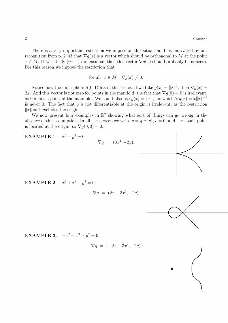
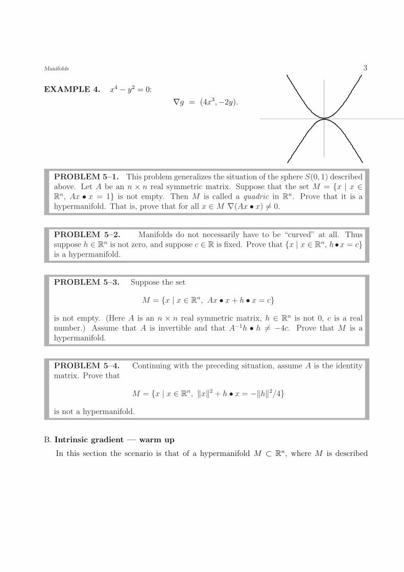
We now present four examples in R2 showing what sort of things can go wrong in theabsence of this assumption. In all these cases we write g = g(x, y), c = 0, and the “bad” pointis located at the origin, so ∇g(0, 0) = 0.

EXAMPLE 1. x3 − y2 = 0:∇g = (3x2,−2y).

EXAMPLE 2. x2 + x3 − y2 = 0:

∇g = (2x + 3x2,−2y).

EXAMPLE 3. −x2 + x3 − y2 = 0:

∇g = (−2x + 3x2,−2y).

Manifolds 3

EXAMPLE 4. x4 − y2 = 0:

∇g = (4x3,−2y).

PROBLEM 5–1. This problem generalizes the situation of the sphere S(0, 1) describedabove. Let A be an n × n real symmetric matrix. Suppose that the set M = {x | x ∈Rn, Ax • x = 1} is not empty. Then M is called a quadric in Rn. Prove that it is ahypermanifold. That is, prove that for all x ∈ M ∇(Ax • x) 6= 0.

PROBLEM 5–2. Manifolds do not necessarily have to be “curved” at all. Thussuppose h ∈ Rn is not zero, and suppose c ∈ R is fixed. Prove that {x | x ∈ Rn, h•x = c}is a hypermanifold.

PROBLEM 5–3. Suppose the set

M = {x | x ∈ Rn, Ax • x + h • x = c}

is not empty. (Here A is an n × n real symmetric matrix, h ∈ Rn is not 0, c is a realnumber.) Assume that A is invertible and that A−1h • h 6= −4c. Prove that M is ahypermanifold.

PROBLEM 5–4. Continuing with the preceding situation, assume A is the identitymatrix. Prove that

M = {x | x ∈ Rn, ‖x‖2 + h • x = −‖h‖2/4}

is not a hypermanifold.

B. Intrinsic gradient — warm up

In this section the scenario is that of a hypermanifold M ⊂ Rn, where M is described

4 Chapter 5

implicitly by the level set

g(x) = 0.

(We can clearly modify g by subtracting a constant from it in order to make M the zero-levelset of g.) We assume ∇g(x) 6= 0 for x ∈ M .

We are definitely thinking that ∇g(x) represents a vector at x ∈ M which is orthogonalto M . We haven’t actually defined this notion yet, but we shall do so in Section F when wetalk about the tangent space to M at x. We’ve discussed this orthogonality on p. 2–43, andit is to our benefit to keep this geometry in mind.

A recurring theme in this chapter is the understanding of the calculus of a function Mf−→ R.

For such a function we do not have the luxury of knowing that f is defined in the ambientspace Rn. As a result, we cannot really talk about partial derivatives ∂f/∂xi. These areessentially meaningless.

For instance, consider the unit circle x2 + y2 = 1 in R2 and the function f defined only onthe unit circle by f(x, y) = x2 − y. We cannot really say that ∂f/∂x = 2x. For we could alsouse the formula f(x, y) = 1 − y2 − y for f , which might lead us to believe ∂f/∂x = 0. Andanyway, the notation ∂f/∂x asks us to “hold y fixed and differentiate with respect to x,” butholding y fixed on the unit circle doesn’t allow x to vary at all.

Nevertheless, we very much want to have a calculus for functions defined on M , and at the

very least we want to be able to define the gradient of Mf−→ R in a sensible way. We shall not

succeed in accomplishing this right away. In fact, this entire chapter is concerned with givingsuch a definition, and we shall finish it only when we reach Section F.

However, we want to handle a very interesting special case right away. Namely, we assume

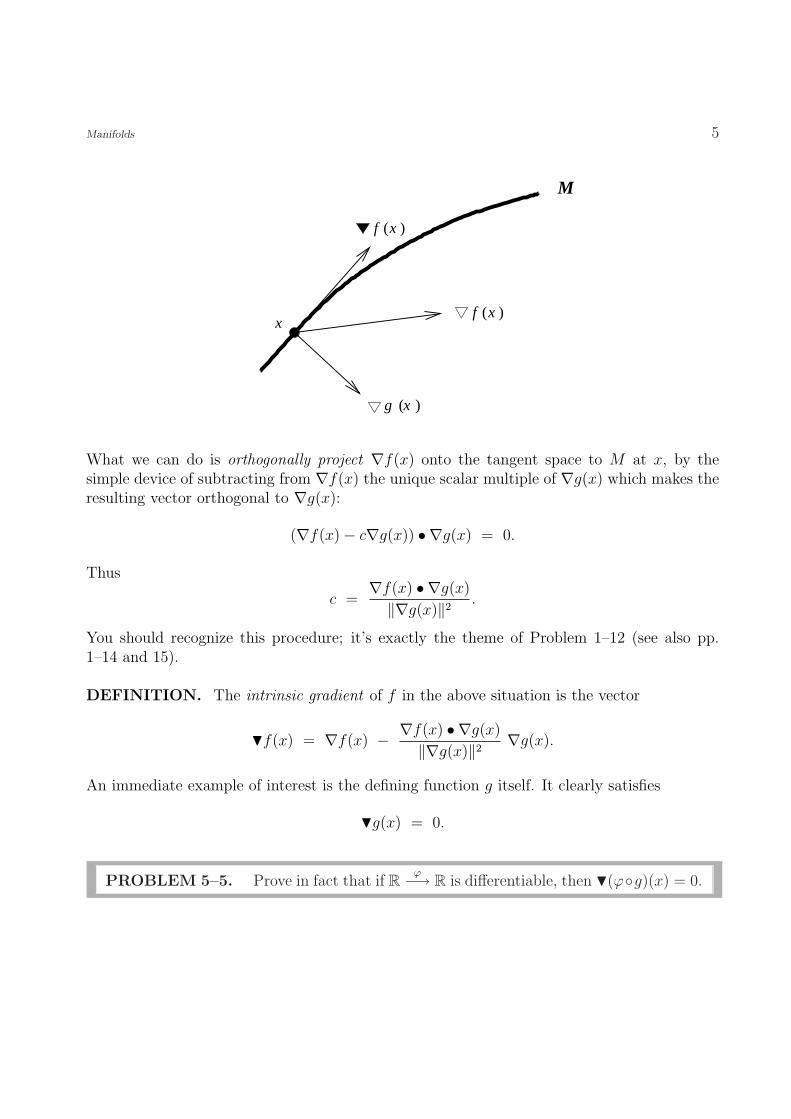
Rn f−→ R, so that f is actually defined in the ambient Rn, and we focus attention on afixed x ∈ M . As such, ∇f(x) ∈ Rn exists, but this is not what we are interested in. Weactually want a vector like ∇f(x) but which is also tangent to M . That is, according to ourexpectations, which is orthogonal to ∇g(x). Here’s a schematic view:

Manifolds 5

( )g x

f x( )x

f x( )

M

What we can do is orthogonally project ∇f(x) onto the tangent space to M at x, by thesimple device of subtracting from ∇f(x) the unique scalar multiple of ∇g(x) which makes theresulting vector orthogonal to ∇g(x):

(∇f(x)− c∇g(x)) • ∇g(x) = 0.

Thus

c =∇f(x) • ∇g(x)

‖∇g(x)‖2.

You should recognize this procedure; it’s exactly the theme of Problem 1–12 (see also pp.1–14 and 15).

DEFINITION. The intrinsic gradient of f in the above situation is the vector

Hf(x) = ∇f(x) − ∇f(x) • ∇g(x)

‖∇g(x)‖2∇g(x).

An immediate example of interest is the defining function g itself. It clearly satisfies

Hg(x) = 0.

PROBLEM 5–5. Prove in fact that if R ϕ−→ R is differentiable, then H(ϕ◦g)(x) = 0.

6 Chapter 5

PROBLEM 5–6. More generally, prove this form of the chain rule:

H(ϕ ◦ f)(x) = ϕ′(f(x))Hf(x).

Our notation H displays the difference between the intrinsic gradient and the ambientgradient ∇. However, it fails to denote which manifold is under consideration. The intrinsicgradient definitely depends on M . Of course, it must depend on M if for no other reasonthan we are computing Hf(x) only if x belongs to M . We illustrate this dependence with thesimple

EXAMPLE. Let M be the sphere S(0, r) in Rn. Then we may use g(x) = ‖x‖2 (or ‖x‖2−r2),so that ∇g = 2x and we obtain the result

Hf(x) = ∇f(x)− x • ∇f(x)

r2x.

PROBLEM 5–7. Let f(x, y) = x2 − y and calculate for the manifold x2 + y2 = 1

Hf = x(2y + 1)(y,−x).

Repeat the exercise for the function h(x, y) = 1− y2 − y, and note that Hf = Hh.

PROBLEM 5–8. The intrinsic gradient in the preceding problem is zero at which fourpoints of the unit circle? Describe the nature of each of these “intrinsic critical points”(local maximum, local minimum, saddle point?). Repeat the entire discussion for thefunction obtained by using the polar angle parameter:

f(cos θ, sin θ) = h(cos θ, sin θ) = cos2 θ − sin θ.

That is, use single variable calculus and the usual first and second deriative with respectto θ.

PROBLEM 5–9. Let 1 ≤ i ≤ n be fixed and let M be the hyperplane {x ∈ Rn | xi =0}. Calculate Hf for this manifold.

Manifolds 7

PROBLEM 5–10. Show that in general

‖Hf(x)‖ = ‖∇f(x)‖ sin θ,

where θ is the angle between the vectors ∇f(x) and ∇g(x).

PROBLEM 5–11. Prove the product rule:

H(fh) = fHh + hHf.

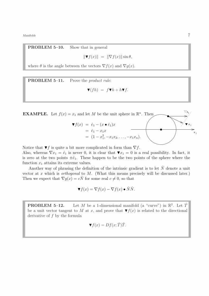
EXAMPLE. Let f(x) = x1 and let M be the unit sphere in Rn. Thenx1

x 1

x 1

Hf(x) = e1 − (x • e1)x

= e1 − x1x

= (1− x21,−x1x2, . . . ,−x1xn).

Notice that Hf is quite a bit more complicated in form than ∇f .Also, whereas ∇x1 = e1 is never 0, it is clear that Hx1 = 0 is a real possibility. In fact, itis zero at the two points ±e1. These happen to be the two points of the sphere where thefunction x1 attains its extreme values.

Another way of phrasing the definition of the intrinsic gradient is to let N denote a unitvector at x which is orthogonal to M . (What this means precisely will be discussed later.)Then we expect that ∇g(x) = cN for some real c 6= 0, so that

Hf(x) = ∇f(x)−∇f(x) • NN .

PROBLEM 5–12. Let M be a 1-dimensional manifold (a “curve”) in R2. Let Tbe a unit vector tangent to M at x, and prove that Hf(x) is related to the directionalderivative of f by the formula

Hf(x) = Df(x; T )T .

8 Chapter 5

PROBLEM 5–13. Suppose Rn f−→ R is homogeneous of degree a. For the manifoldwhich is the sphere S(0, r) of radius r show that

Hf = ∇f − afx

r2.

Another extremely important property is the fact that Hf is truly intrinsic: it dependsonly on the knowledge of f when restricted to the manifold. This is not quite clear at thepresent stage of our development because we have employed the ambient gradient ∇f in ourdefinition. However, the following argument should serve to make it intuitively clear. Inorder that Hf just depend on the function f restricted to M , it must be the case that twofunctions which are equal on M turn out to have the same intrinsic gradient. Equivalently,their difference has zero intrinsic gradient. Equivalently, if f = 0 on M , then Hf = 0 on M .This seems reasonable, as we believe that if M is a level set of f , then ∇f must be orthogonalto M ; that is, ∇f is a scalar multiple of ∇g. But then the orthogonal projection of ∇forthogonal to ∇g is zero: Hf = 0.

Rather than continuing with this discussion at the present time, we instead turn to somewonderful numerical calculations.

C. Intrinsic critical points

We continue with the notation and ideas of Section B, so that M is a hypermanifold in Rn

described by an equation g(x) = 0. We say that x ∈ M is an intrinsic critical point of f ifHf(x) = 0. That is,

∇f(x) =∇f(x) • ∇g(x)

‖∇g(x)‖2∇g(x).

This is a rather daunting equation to solve for x, but it helps to notice that it says preciselythat ∇f(x) equals a scalar times ∇g(x); for then taking the inner product with ∇g(x) showsthat the scalar must be the one displayed. This scalar λ is called a Lagrange multiplier forthe problem. We then are required to solve the equations

{∇f(x) = λ∇g(x),

g(x) = 0 (as x ∈ M).

The “unknowns” are both x and λ. If we count scalar unknowns and equations, we have n + 1unknowns x1, . . . , xn, λ, as well as n + 1 equations. Hopeful!

The equation g(x) = 0 is often referred to as the constraint.

Manifolds 9

As is usual in similar situations, setting up the equations is the easy part. Solving them isthe hard part, as they are usually nonlinear. Here are some examples.

EXAMPLE. Find the intrinsic critical points of f(x, y) = x(y − 1) on the unit circlex2 + y2 = 1.Solution. To eliminate some “2’s” we can use g(x, y) = 1

2(x2 + y2 − 1). Then the Lagrange

formulation is: {(y − 1, x) = λ(x, y),

x2 + y2 = 1.

Thus y − 1 = λx and x = λy. Thus

y − 1 = λ2y,

soy(λ2 − 1) = −1.

Thus

y =−1

λ2 − 1, x =

−λ

λ2 − 1.

Finally, the constraint givesλ2 + 1

(λ2 − 1)2= 1.

Thus

λ2 + 1 = (λ2 − 1)2

= λ4 − 2λ2 + 1;

λ4 = 3λ2.

Thus λ = 0 or λ2 = 3. These give three points:

λ = 0 : (0, 1);

λ =√

3 :

(−√3

2,−1

2

);

λ = −√

3 :

(√3

2,−1

2

).

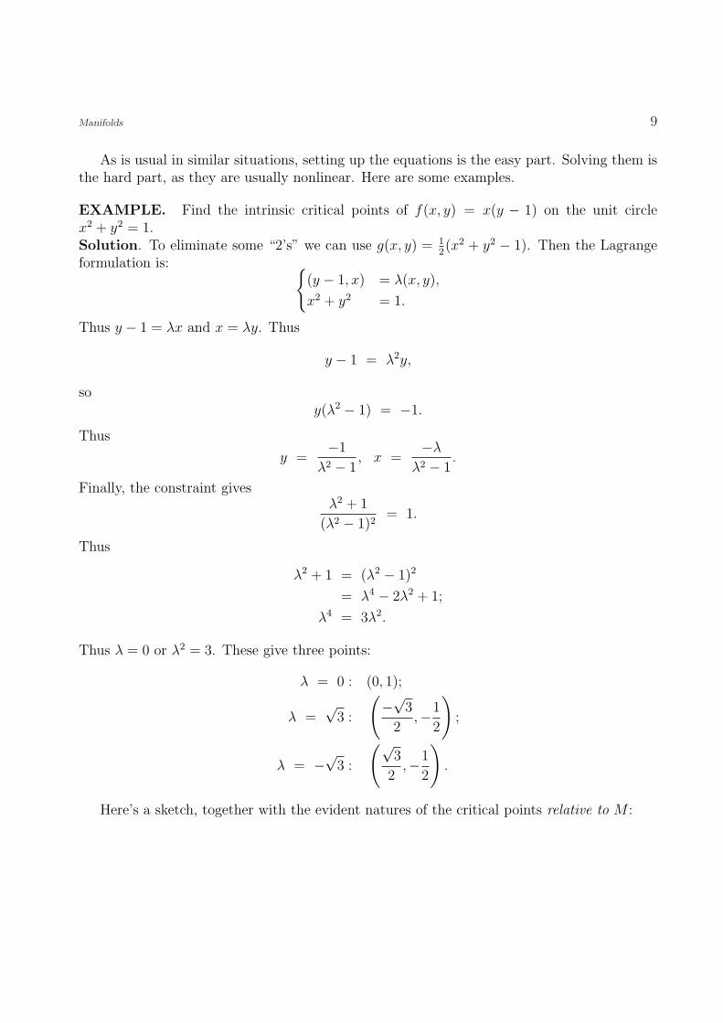
Here’s a sketch, together with the evident natures of the critical points relative to M :

10 Chapter 5

3 3

4

MAX MIN

SADDLE

f = f =

f = 0

3 3

4−

Notice, by the way, that (0, 1) is actually an ambient critical point of f : ∇f(0, 1) = (0, 0). Itis the only one.

PROBLEM 5–14. Just as in Problem 5–8, analyze the function we just studied byexamining the function cos θ(sin θ − 1).

EXAMPLE. Find the intrinsic critical points of f(x, y) = x3 + 8y on the ellipsex2

4+ y2

2= 1.

Solution. The Lagrange formulation is:

3x2 = λx/2,

8 = λy,x2

4+ y2

2= 1.

If x = 0, we get y2 = 2 and thus two points: (0,√

2), (0,−√2). If x 6= 0, then

x =λ

6, y =

8

λ.

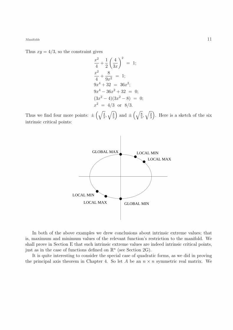
Manifolds 11

Thus xy = 4/3, so the constraint gives

x2

4+

1

2

(4

3x

)2

= 1;

x2

4+

8

9x2= 1;

9x4 + 32 = 36x2;

9x4 − 36x2 + 32 = 0;

(3x2 − 4)(3x2 − 8) = 0;

x2 = 4/3 or 8/3.

Thus we find four more points: ±(√

43,√

43

)and ±

(√83,√

23

). Here is a sketch of the six

intrinsic critical points:

GLOBAL MAX

LOCAL MAX

LOCAL MIN

LOCAL MIN

LOCAL MAX

GLOBAL MIN

In both of the above examples we drew conclusions about intrinsic extreme values; thatis, maximum and minimum values of the relevant function’s restriction to the manifold. Weshall prove in Section E that such intrinsic extreme values are indeed intrinsic critical points,just as in the case of functions defined on Rn (see Section 2G).

It is quite interesting to consider the special case of quadratic forms, as we did in provingthe principal axis theorem in Chapter 4. So let A be an n × n symmetric real matrix. We

12 Chapter 5

there were analyzing A by means of the Rayleigh quotient

Ax • x

‖x‖2,

and we essentially found its critical points in Rn. The homogeneity shows that to be the sameas finding the intrinsic critical points of Ax • x on the unit sphere. Thus we ask for points xsatisfying

H(Ax • x) = 0 and ‖x‖ = 1.

The Lagrange formulation gives

{∇(Ax • x) = λ∇(‖x‖2),

‖x‖ = 1.

That is, {Ax = λx,

‖x‖ = 1.

Thus the intrinsic critical points of Ax • x on the unit sphere are precisely the eigenvectors ofA! As an example of this procedure, work out the following problem:

PROBLEM 5–15. Find the intrinsic critical points of (x + y)(y + z) on the unitsphere x2 + y2 + z2 = 1.

PROBLEM 5–16. For the Rayleigh quotient function Q(x) = Ax •x/‖x‖2 show thatthe intrinsic gradient on the unit sphere equals

HQ = ∇Q

= 2Ax− 2Ax • xx.

Here are six more or less routine exercises, followed by six challenging ones.

PROBLEM 5–17. Use the Lagrange technique to find the points on the parabolay2 + 2x = 8 which are closest to the origin.

PROBLEM 5–18. Find the minimum of x4+4axy+y4 on the hyperbola x2−y2 = 1.

Manifolds 13

PROBLEM 5–19. Find the minimum distance from (9, 12,−5) to points on the conein R3 given by 4z2 = x2 + y2.

PROBLEM 5–20. Consider the function f(x, y) = x on the level set y2−x3 = 0. Showthat f attains its minimum value at the origin only. Show that the Lagrange formulationfails to produce this result. Explain why.

PROBLEM 5–21. Repeat the preceding exercise for the function f(x, y) = y onthe set M : y3 = x6 + x8. In this case show also that the level set M is a bona fide1-dimensional manifold in R2.

PROBLEM 5–22. Let a, b, c be positive constants. Find the intrinsic critical pointsof a

x+ b

y+ c

zon the unit sphere x2 + y2 + z2 = 1.

PROBLEM 5–23. Find the intrinsic critical points of 2(x1 + x2 + x3)(x1 + x2 + x4)on the unit sphere in R4.

PROBLEM 5–24. Find all the intrinsic critical points of f(x) = x31+x3

2+x33+2x1x2x3

on the unit sphere in R3.

PROBLEM 5–25*. Find all the intrinsic critical points of f(x) = x31+x3

2+x33−3x1x2x3

on the unit sphere in R3.

PROBLEM 5–26**. Let a be an arbitrary but fixed real number. Find all the intrinsiccritical points of f(x) = x3

1 + x32 + x3

3 + ax1x2x3 on the unit sphere in R3, and count howmany there are depending on the value of a.

PROBLEM 5–27. Find all the intrinsic critical points of f(x) = x31 + x2

2 + x3 on theunit sphere in R3. Determine the maximum and minimum values of f on the sphere.

The next problem is a gem I found in the book Ideals, Varieties, and Algorithms, by Cox,

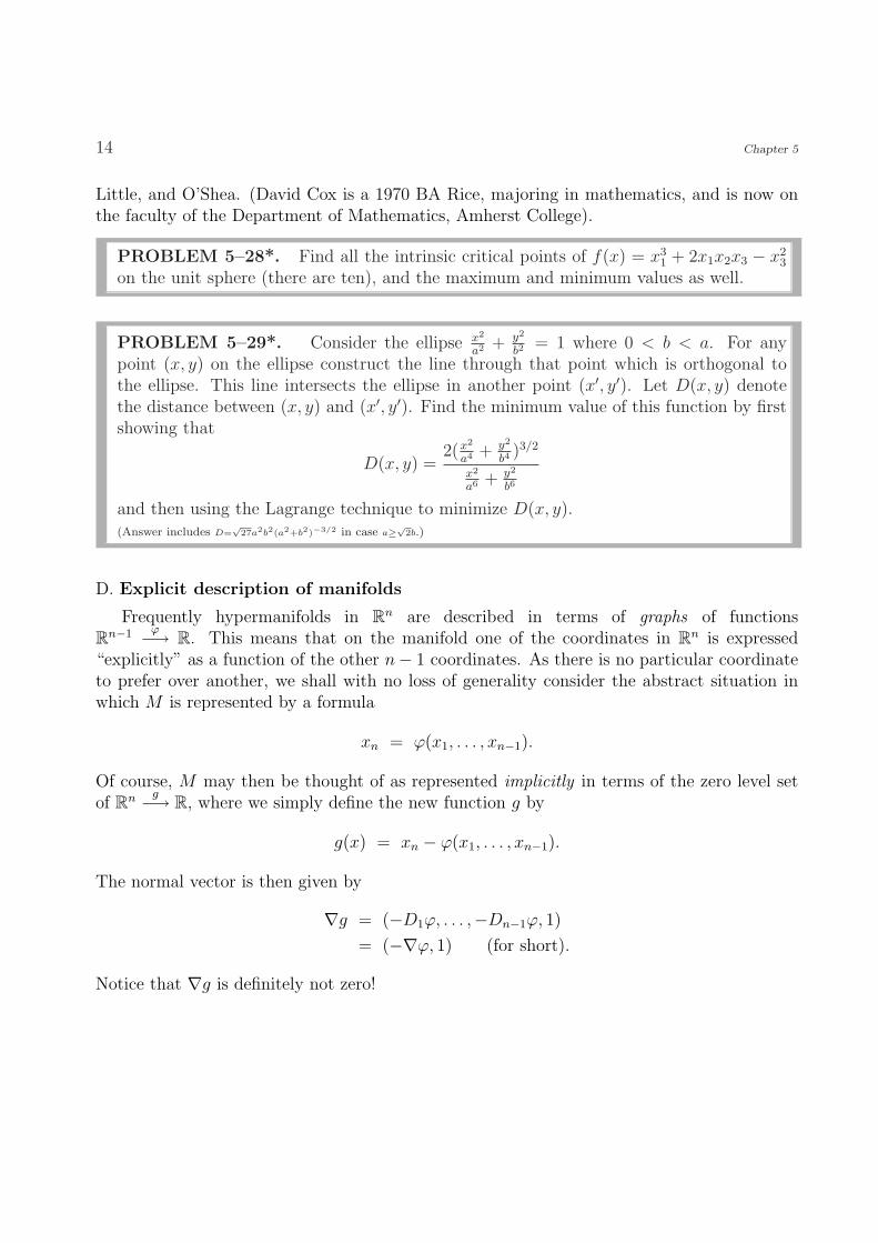
14 Chapter 5

Little, and O’Shea. (David Cox is a 1970 BA Rice, majoring in mathematics, and is now onthe faculty of the Department of Mathematics, Amherst College).

PROBLEM 5–28*. Find all the intrinsic critical points of f(x) = x31 + 2x1x2x3 − x2

3

on the unit sphere (there are ten), and the maximum and minimum values as well.

PROBLEM 5–29*. Consider the ellipse x2

a2 + y2

b2= 1 where 0 < b < a. For any

point (x, y) on the ellipse construct the line through that point which is orthogonal tothe ellipse. This line intersects the ellipse in another point (x′, y′). Let D(x, y) denotethe distance between (x, y) and (x′, y′). Find the minimum value of this function by firstshowing that

D(x, y) =2(x2

a4 + y2

b4)3/2

x2

a6 + y2

b6

and then using the Lagrange technique to minimize D(x, y).(Answer includes D=

√27a2b2(a2+b2)−3/2 in case a≥√2b.)

D. Explicit description of manifolds

Frequently hypermanifolds in Rn are described in terms of graphs of functionsRn−1 ϕ−→ R. This means that on the manifold one of the coordinates in Rn is expressed“explicitly” as a function of the other n− 1 coordinates. As there is no particular coordinateto prefer over another, we shall with no loss of generality consider the abstract situation inwhich M is represented by a formula

xn = ϕ(x1, . . . , xn−1).

Of course, M may then be thought of as represented implicitly in terms of the zero level setof Rn g−→ R, where we simply define the new function g by

g(x) = xn − ϕ(x1, . . . , xn−1).

The normal vector is then given by

∇g = (−D1ϕ, . . . ,−Dn−1ϕ, 1)

= (−∇ϕ, 1) (for short).

Notice that ∇g is definitely not zero!

Manifolds 15

Now we give an interesting calculation to show what Hf looks like in this framework. Weshall require only the values of the function f on the manifold M . A convenient way to usethese values is to define an associated function f0 on Rn−1 by the formula

f0(x1, . . . , xn−1) = f(x1, . . . , xn−1, ϕ(x1, . . . , xn−1)

).

Notice that the new function f0 indeed uses only the evaluation of f at points of M .Note first that the chain rule implies

Dkf0 = Dkf + DnfDkϕ, 1 ≤ k ≤ n− 1.

Using vector notation in Rn−1,

∇f0 = (D1f0, . . . , Dn−1f0)

= (D1f, . . . , Dn−1f) + Dnf(D1ϕ, . . . , Dn−1ϕ).

Now we simply regard ∇f0 as a vector in Rn with nth component 0, which we write as

0 = Dnf + Dnf(−1).

Thus

∇f0 = (D1f, . . . , Dn−1f, Dnf) + Dnf(D1ϕ, . . . , Dn−1ϕ,−1)

= ∇f + Dnf(∇ϕ,−1)

= ∇f −Dnf∇g.

Now we are all set to compute the intrinsic gradient of f . By definition

Hf = ∇f − ∇f • ∇g

‖∇g‖2∇g

= ∇f − (∇f0 + Dnf∇g) • ∇g

‖∇g‖2∇g

= ∇f − ∇f0 • ∇g

‖∇g‖2∇g −Dnf∇g

= ∇f0 − ∇f0 • ∇g

‖∇g‖2∇g.

We summarize:

16 Chapter 5

THEOREM. In the above context, where M is given explicitly

M = {x ∈ Rn | xn = ϕ(x1, . . . , xn−1)},we define

f0(x1, . . . , xn−1) = f(x1, . . . , xn−1, ϕ(x1, . . . , xn−1)

).

Then

Hf = ∇f0 +∇f0 • ∇ϕ

‖∇ϕ‖2 + 1(−∇ϕ, 1).

In particular, the intrinsic gradient Hf depends only on the restriction off to M .

This theorem is of great theoretical importance in that it shows dramatically the intrinsicnature of Hf . However, it does not appear to be of any particular use in solving exercises, asthe Lagrange formulation of the preceding section is indeed quite applicable.

PROBLEM 5–30. Prove that f has an intrinsic critical point at x ⇐⇒ f0 has acritical point at the corresponding point.

E. Implicit function theorem

We now turn to a theorem of immense importance in the study of manifolds. It actuallyprovides the complete understanding of intrinsic gradients. More than that, it shows thathypermanifolds which are described implicitly can also be described explicitly . Thus it is wellnamed: THE IMPLICIT FUNCTION THEOREM.

We do not prove this theorem (one of the “hard” ones) in this course. It is commonly provedin beginning courses in mathematical analysis. However, we very much need to understandexactly what it does (and does not) say.

Suppose then that the hypermanifold M ⊂ Rn is described implicitly in a neighborhoodof x0 ∈ M by the equation

g(x) = 0.

As usual, Rn g−→ R is assumed to be of class C1, and ∇g(x) 6= 0 for all x in a neighborhoodof x0. We want to describe M explicitly near x0, so what we need to do is solve the equationg(x) = 0 for one of the variables in terms of the others. Say we succeed in solving for xn as afunction of x1, . . . , xn−1: in a neighborhood of x0 we then have a situation

g(x) = 0 ⇐⇒ xn = ϕ(x1, . . . , xn−1),

for some function ϕ defined on a neighborhood in Rn−1.

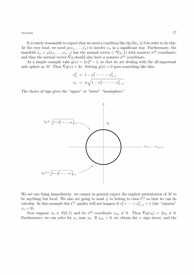
Manifolds 17

It is surely reasonable to expect that we need a condition like ∂g/∂xn 6= 0 in order to do this.At the very least, we need g(x1, . . . , xn) to involve xn in a significant way. Furthermore, themanifold xn = ϕ(x1, . . . , xn−1) has the normal vector (−∇ϕ, 1) with nonzero nth coordinate,and thus the normal vector ∇g should also have a nonzero nth coordinate.

As a simple example take g(x) = ‖x‖2 − 1, so that we are dealing with the all-importantunit sphere as M . Then ∇g(x) = 2x. Solving g(x) = 0 goes something like this:

x2n = 1− x2

1 − · · · − x2n−1

xn = ±√

1− x21 − · · · − x2

n−1.

The choice of sign gives the “upper” or “lower” “hemisphere.”

nx = −

xn = 2

n−1x− ... −

2n−1

x− ... −

xn

x 1 n − 1 , ... , x

1 − x12

1 − x12

We see one thing immediately: we cannot in general expect the explicit presentation of M tobe anything but local. We also are going to want ϕ to belong to class C1 so that we can docalculus. In this example this C1 quality will not happen if x2

1 + · · ·+x2n−1 = 1 (the “equator”

xn = 0).Now suppose x0 ∈ S(0, 1) and its nth coordinate xon 6= 0. Then ∇g(x0) = 2x0 6= 0.

Furthermore, we can solve for xn near x0. If xon > 0, we obtain the + sign above, and the

18 Chapter 5

reverse if xon < 0. Thus in the latter case xon < 0, we have

xn = −√

1− x21 − · · · − x2

n−1 for x21 + · · ·+ x2

n−1 < 1.

Of course, the entire sphere can be handled in a similar way since ∇g(x0) = 2x0 6= 0 requiressome coordinate xoi of x0 to be nonzero, and we can then solve for xi locally:

xi = ±√

1− x21 − · · · − x2

i−1 − x2i+1 − · · · − x2

n.

The above simple example of the sphere is completely typical. Here is the result.

IMPLICIT FUNCTION THEOREM. Suppose the hypermanifold M ⊂ Rn is describedas the level set

g(x) = 0,

where Rn g−→ R is of class C1 and ∇g 6= 0 on M . Suppose x0 ∈ M . Suppose that ∂g/∂xi(x0) 6=0. Then there exists Rn−1 ϕ−→ R of class C1 such that for all x in a sufficiently smallneighborhood of x0,

g(x) = 0 ⇐⇒ xi = ϕ(x1, . . . , xi−1, xi+1, . . . , xn).

Though this is an existence theorem and as such does not provide a clue about the actualcalculation of ϕ, the chain rule gives “explicit” formulas for the partial derivatives of ϕ. Forwe may start with the functional identity in the variables x1, . . . , xi−1, xi+1, . . . , xn:

g(x1, . . . , xi−1, ϕ, xi+1, . . . , xn) = 0.

Now differentiate this identity with respect to xj for any j 6= i. The chain rule implies

Djg + DigDjϕ = 0.

Therefore we conclude that

Djϕ = −Djg

Dig.

On the right side of the latter equation, the partial derivatives of g are evaluated at xi = ϕ.Notice the appearance of the nonzero quantity Dig in the denominator.

There is a nice moral to get from all of this. Solving the equation g(x) = 0 for xi in termsof the other coordinates is likely to be a very difficult task. But once that has been done andthe above function ϕ has been produced, the calculation of the partial derivatives Djϕ is verysimple. In fact, it’s a linear task. You have seen this sort of “implicit differentiation” in your

Manifolds 19

introductory calculus courses. For instance there are lots of exercises of the following nature:the equation

πexy + sin y − y − x2 = 0

is satisfied by a function y = y(x) near x = 0, and y(0) = π. Compute dy/dx. The solutionis obtained by performing d/dx:

πexy

(x

dy

dx+ y

)+ cos y

dy

dx− dy

dx− 2x = 0.

Then solve:dy

dx=

2x− πyexy

πxexy + cos y − 1.

How simple. (Never mind that we don’t really “know” the terms y = y(x) on the right side.)Notice that when x = 0 and y = π, the denominator equals −2 and this is not 0. In particular,

dy

dx

∣∣∣x=0

=π2

2.

Another nice result of the implicit function theorem is the proof that the intrinsic gradientHf depends only on M and not on the particular function g whose level set is equal to M .This is clear once we check that ∇g is uniquely determined by M , up to a nonzero scalarmultiple; for the formula for Hf shows that the scalar multiple cancels out of the equation.More geometrically, Hf is just the vector ∇f with the correct multiple of ∇g added so thatthe resulting vector is orthogonal to ∇g; this makes it clear that only the direction of ∇g isneeded.

THEOREM. Given a hypermanifold M ⊂ Rn, suppose it is described as the level set {x ∈Rn | g(x) = 0}, where ∇g 6= 0. Then ∇g is uniquely determined by M , up to a nonzero scalarmultiple (which may be a function of x).

PROOF. Suppose for instance that Dng(x0) 6= 0. Then the implicit function theorem yields

a function Rn−1 ϕ−→ R such that near x0 we have

x ∈ M ⇐⇒ xn = ϕ(x1, . . . , xn−1).

Then as above we obtain on M

Djg + DngDjϕ = 0, 1 ≤ j ≤ n− 1.

We conclude∇g = Dng(−∇ϕ, 1).

20 Chapter 5

If another function g also gives the manifold, and∇g(x0) 6= 0, then g(x1, . . . , xn−1, ϕ(x1, . . . , xn−1)) =0 so that the chain rule again gives

∇g = Dng(−∇ϕ, 1).

Thus Dng(x) 6= 0 and ∇g(x) =scalar times ∇g(x).QED

We can now clear up an issue that we have been ignoring, thanks to the fact that weunderstand that the intrinsic gradient Hf is completely determined by the restriction of thefunction f to the manifold in question. The issue is this: suppose f attains a local maximumor minimum value at x0 ∈ M relative to the restriction of f to M . Then we want to knowthat necessarily x0 is an intrinsic critical point of f . Here’s the result:

THEOREM. Suppose M is a hypermanifold in Rn and suppose Rn f−→ R is a C1 functiondefined in a neighborhood of a point x0 ∈ M . Suppose that f(x) ≤ f(x0) for all x ∈ Mbelonging to some neighborhood of x0. Then Hf(x0) = 0.

PROOF. Thanks to the implicit function theorem, we know that M can be representedexplicitly near x0 by an equation of the form

xn = ϕ(x1, . . . , xn−1)

(we have named xn as the distinguished coordinate for simplicity of writing only). We use thefunction f0 of Section D,

f0(x1, . . . , xn−1) = f(x1, . . . , xn−1, ϕ(x1, . . . , xn−1)).

Let x′0 = (x01, . . . , x0,n−1). Then our hypothesis means precisely that

f0(x′) ≤ f0(x

′0)

for all x′ ∈ Rn−1 sufficiently near x′0. Thus x′0 is a critical point for the function f0, and weconclude that its gradient ∇f0(x

′0) = 0. But then the theorem on p. 5–15 yields

Hf(x0) = ∇f0 +∇f0 • ∇ϕ

‖∇ϕ‖2 + 1(−∇ϕ, 1)

= 0.

QED

Manifolds 21

REMARKS. Of course, the conclusion still holds if we are dealing with a local minimuminstead: f(x) ≥ f(x0) for all x ∈ M sufficiently near x0. In the next section we shall give asomewhat different proof of this result that is even more intrinsic. And in Section G we shalllearn that the theorem remains valid for manifolds M ⊂ Rn of any dimension, not just n− 1.

PROBLEM 5–31. THE ARITHMETIC-GEOMETRIC MEAN INEQUALITY.Using the following outline, prove that for any x1 ≥ 0, . . . , xn ≥ 0,

(x1 . . . xn)1/n ≤ x1 + · · ·+ xn

n,

and that equality holds ⇐⇒ x1 = · · · = xn.

a. Prove first that you may assume that x1 + · · ·+ xn = 1.

b. Show that the function f = x1 . . . xn restricted to the set x1 + · · ·+ xn = 1, xi ≥ 0for all i, attains its maximum value at some x0.

c. Show that all the coordinates of this point x0 are positive.

d. Use the Lagrange technique to determine x0.

PROBLEM 5–32. Find the minimum of x1 x2 . . . xn subject to the constraint

1

x1

+1

x2

+ · · ·+ 1

xn

= 1, all xi > 0.

F. The tangent space

Now we are going to face the problem of actually defining tangent vectors to a manifold.Suppose that M ⊂ Rn is a manifold, not necessarily a hypermanifold. Suppose x0 ∈ M . Wewant to give a definition of tangent vectors to M at x0 that is as intrinsic to M as possible(how the “inhabitants” of M view tangent vectors). We shall accomplish this by focusingattention on curves which lie in the manifold.

DEFINITION. In the above situation consider all curves (see p. 2–3) γ from R to Rn which

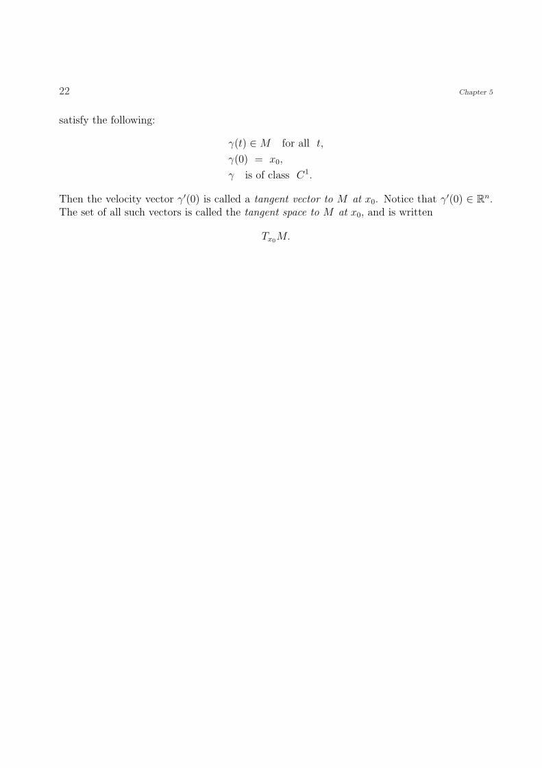
22 Chapter 5

satisfy the following:

γ(t) ∈ M for all t,

γ(0) = x0,

γ is of class C1.

Then the velocity vector γ′(0) is called a tangent vector to M at x0. Notice that γ′(0) ∈ Rn.The set of all such vectors is called the tangent space to M at x0, and is written

Tx0M.

Manifolds 23

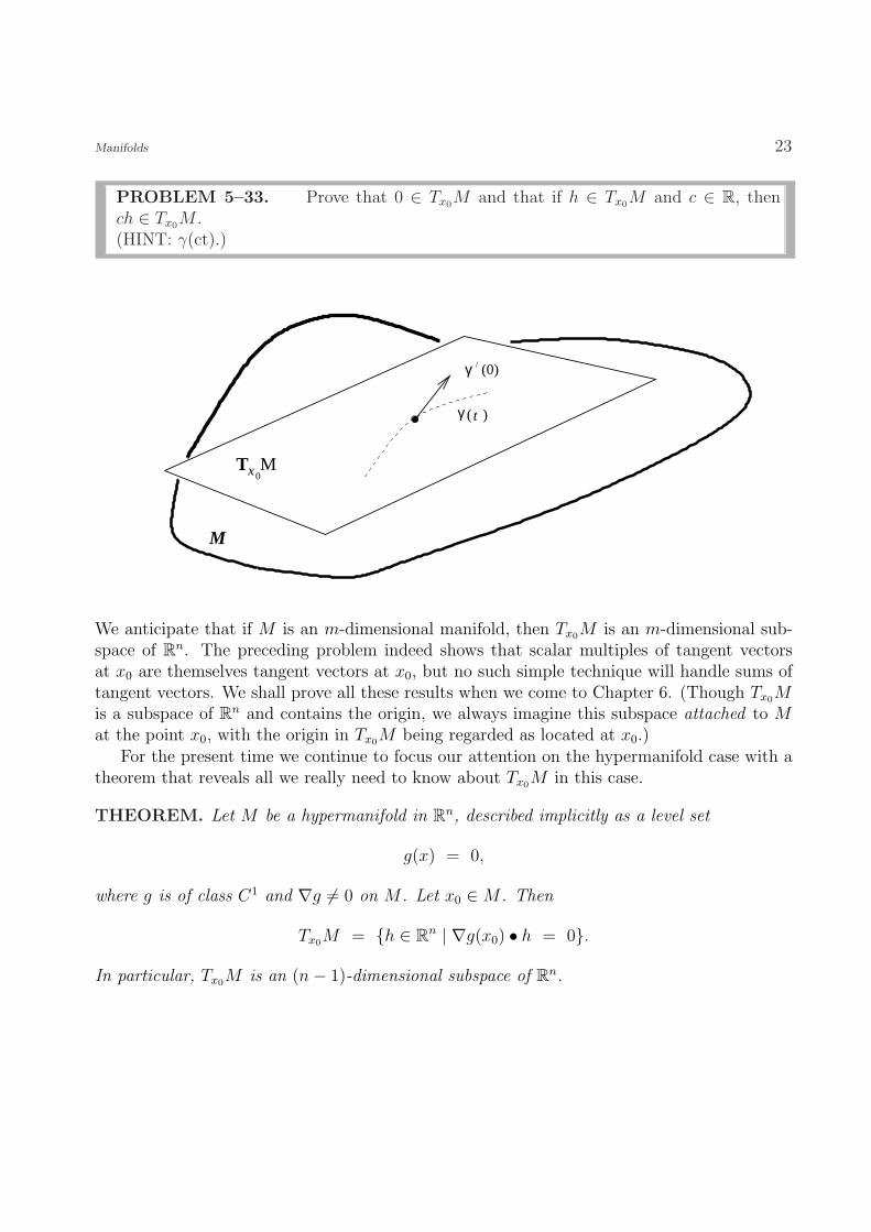
PROBLEM 5–33. Prove that 0 ∈ Tx0M and that if h ∈ Tx0M and c ∈ R, thench ∈ Tx0M .(HINT: γ(ct).)

M

γ

Tx0M

(0)

t( )γ

We anticipate that if M is an m-dimensional manifold, then Tx0M is an m-dimensional sub-space of Rn. The preceding problem indeed shows that scalar multiples of tangent vectorsat x0 are themselves tangent vectors at x0, but no such simple technique will handle sums oftangent vectors. We shall prove all these results when we come to Chapter 6. (Though Tx0Mis a subspace of Rn and contains the origin, we always imagine this subspace attached to Mat the point x0, with the origin in Tx0M being regarded as located at x0.)

For the present time we continue to focus our attention on the hypermanifold case with atheorem that reveals all we really need to know about Tx0M in this case.

THEOREM. Let M be a hypermanifold in Rn, described implicitly as a level set

g(x) = 0,

where g is of class C1 and ∇g 6= 0 on M . Let x0 ∈ M . Then

Tx0M = {h ∈ Rn | ∇g(x0) • h = 0}.

In particular, Tx0M is an (n− 1)-dimensional subspace of Rn.

24 Chapter 5

PROOF. First, suppose h ∈ Tx0M . Use a curve γ as in the definition above, with γ′(0) = h.Then since γ(t) ∈ M ,

g(γ(t)) = 0.

Computing the t derivative and using the chain rule,

∇g(γ(t)) • γ′(t) = 0.

Setting t = 0,

∇g(x0) • h = 0.

Conversely, suppose h ∈ Rn satisfies

∇g(x0) • h = 0.

Now we have to do something quite significant. We are required to produce a curve in Mwith all the right properties. Since we don’t even know how to produce individual points inM , much less a whole curve, we need a theorem of some sort. The implicit function theoremserves the purpose perfectly. For ease in writing let us suppose Dng(x0) 6= 0. Then we know(thanks to the implicit function theorem) that M can be described explicitly as a graph

xn = ϕ(x1, . . . , xn−1)

near x0. Write x0 = (x01, . . . , x0n). We then define a curve γ(t) by making it affine in the“independent” coordinates x1, . . . , xn−1 in the following way:

γj(t) = x0j + hjt, 1 ≤ j ≤ n− 1,

γn(t) = ϕ (γ1(t), . . . , γn−1(t)) .

From the chain rule and the formula on p. 5–18 we obtain

γ′n(0) =n−1∑j=1

Djϕ (x01, . . . , x0,n−1) γ′j(0)

=n−1∑j=1

− Djg(x0)

Dng(x0)hj.

But also we have

∇g(x0) • h = 0;

Manifolds 25

that is,n−1∑j=1

Djg(x0)hj + Dng(x0)hn = 0.

Thusγ′n(0) = hn.

This proves that γ′(0) = h, as desired.QED

As a nice bonus, we can now easily give a complete understanding of the intrinsic gradient

of a function, relative to the hypermanifold M . Suppose first that Rn f−→ R is of class C1 neara point x0 ∈ M . Suppose that h ∈ Tx0M . There are now two ways to view this situation.

(1) We use ∇g(x0) • h = 0 and the definition from p. 5–5,

Hf(x0) = ∇f(x0)− ∇f(x0) • ∇g(x0)

‖∇g(x0)‖2∇g(x0),

to conclude that

Hf(x0) • h = ∇f(x0) • h

= Df(x0; h).

Remember from p. 2–14 that Df(x0; h) is our notation for the directional derivativeof f at x0 in the direction h. Thus Hf(x0) is the unique vector in Tx0M whose innerproduct with every h ∈ Tx0M equals Df(x0; h).

(2) Consider an arbitrary curve γ in M such that γ(0) = x0 and γ′(0) = h. Then the chainrule gives

d

dtf (γ(t)) = ∇f (γ(t)) • γ′(t),

so that

d

dtf (γ(t))

∣∣∣t=0

= ∇f(x0) • h

= Hf(x0) • h.

It is this second relationship that is so intriguing, since the function f ◦ γ depends on thebehavior of f only on the manifold M and not on the ambient Rn. We can therefore extendthe definition of p. 5–5 as in the theorem we are preparing to consider.

26 Chapter 5

But before we state the theorem, we need to explain part of the hypothesis. Namely, we

are going to assume that Mf−→ R is of class C1. Since f might be defined only on M , it is not

immediately clear how to define this continuous differentiability. In fact, a moment’s thoughtmight lead to two competing ideas:

(1) Representing M in an explicit manner such as

xn = ϕ(x1, . . . , xn−1),

require the resulting function

f0(x1, . . . , xn−1) = f(x1, . . . , xn−1, ϕ(x1, . . . , xn−1))

to be of class C1 on (a neighborhood in) Rn.

(2) Require that there exist a C1 function Rn F−→ R such that F (x) = f(x) for x ∈ M (ina neighborhood of some point).

PROBLEM 5–34. Prove that these two definitions are equivalent.

THEOREM. Let M be a hypermanifold in Rn and x0 ∈ M . Let Mf−→ R be a C1 function

defined only on M . Then there exists a unique vector Hf(x0) in Tx0M such that for all C1

curves γ in M such that γ(0) = x0,

d

dtf (γ(t))

∣∣∣t=0

= Hf(x0) • γ′(0).

DEFINITION. The tangent vector Hf(x0) is called the intrinsic gradient of f at x0.Because of the discussion right before the theorem, it agrees with the definition given onp. 5–5 in case f is defined in a neighborhood of x0 in Rn.

PROOF. Use the second of the two definitions of C1 given above. Thus in a neighborhood

of x0 there exists some C1 function Rn F−→ R which agrees with f on M . Then we simplycompute

d

dtf (γ(t))

∣∣∣t=0

=d

dtF (γ(t))

∣∣∣t=0

= HF (x0) • γ′(0),

Manifolds 27

thanks to the known properties of the intrinsic gradient HF (x0) of the ambient function F .This finishes the existence part of the proof, as we may simply define Hf(x0) = HF (x0).

The uniqueness is a separate argument. If there were two vectors v and w ∈ Tx0M fulfillingthe conclusion of the theorem, then we would have

v • γ′(0) = w • γ′(0) for all curves γ.

Thus,(v − w) • h = 0 for all h ∈ Tx0M.

Since v − w ∈ Tx0M , we conclude that v − w = 0. Thus v = w.QED

REMARK. Given a C1 function Mf−→ R, there are many ways to extend it to Rn F−→ R in

a neighborhood of x0. Each such F has a gradient ∇F (x0), but the intrinsic gradient HF (x0)is independent of the choice of the extension F . Our results show that each HF (x0) is justequal to Hf(x0). Thus we have a very practical “algorithm” for computing Hf . Namely, firstextend f to an ambient C1 function F ; second, compute HF . The resulting vector is preciselyHf .

The above results are in agreement with what we accomplished in the theorem on p. 5–15,where we noticed that the intrinsic gradient of a function depends only on its restriction tothe manifold. The extra information we now have comes from the intrinsic understanding oftangent vectors themselves.

G. Manifolds that are not hyper

In this section we want to move away from the restriction that M ⊂ Rn has dimensionn− 1. Thus we shall study manifolds of dimension m contained in Rn, where 1 ≤ m ≤ n− 1.This range of dimension covers all that we are really concerned with in the present chapter,going from m = 1 (“curves”) to m = 2 (“surfaces”) on up to m = n−1 (hypermanifolds). Wedo not deal with m = 0, as 0-dimensional “manifolds” would just consist of isolated points inRn, and no actual calculus could be done. At the other extreme, m = n, we would be talkingabout n-dimensional manifolds contained in Rn and these are simply open subsets of Rn. Thisleads essentially to the “flat” calculus we have studied in detail in Chapters 2–4 and presentsno new ideas at the present time.

Again we shall use both an implicit presentation and an explicit presentation of M . Inaddition we shall also consider a third method, a parametric presentation. Here is a preliminarysummary:

IMPLICIT M is defined by n−m constraints placed on the points of Rn.

28 Chapter 5

EXPLICIT M is defined by giving n−m coordinates of Rn as explicitfunctions of the other m coordinates.

PARAMETRIC M is defined by describing its points as a function of mother real variables (called parameters).

We devote the rest of this section to the discussion of three examples which happen to bequite interesting manifolds.

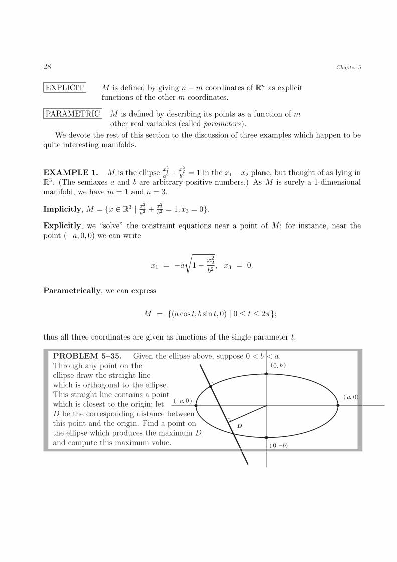
EXAMPLE 1. M is the ellipsex21

a2 +x22

b2= 1 in the x1−x2 plane, but thought of as lying in

R3. (The semiaxes a and b are arbitrary positive numbers.) As M is surely a 1-dimensionalmanifold, we have m = 1 and n = 3.

Implicitly, M = {x ∈ R3 | x21

a2 +x22

b2= 1, x3 = 0}.

Explicitly, we “solve” the constraint equations near a point of M ; for instance, near thepoint (−a, 0, 0) we can write

x1 = −a

√1− x2

2

b2, x3 = 0.

Parametrically, we can express

M = {(a cos t, b sin t, 0) | 0 ≤ t ≤ 2π};

thus all three coordinates are given as functions of the single parameter t.

PROBLEM 5–35. Given the ellipse above, suppose 0 < b < a.Through any point on theellipse draw the straight linewhich is orthogonal to the ellipse.This straight line contains a pointwhich is closest to the origin; let 0

0 a,

b

0, −b

D

−a, ( )

( )

( )

0, ( )

D be the corresponding distance betweenthis point and the origin. Find a point onthe ellipse which produces the maximum D,and compute this maximum value.

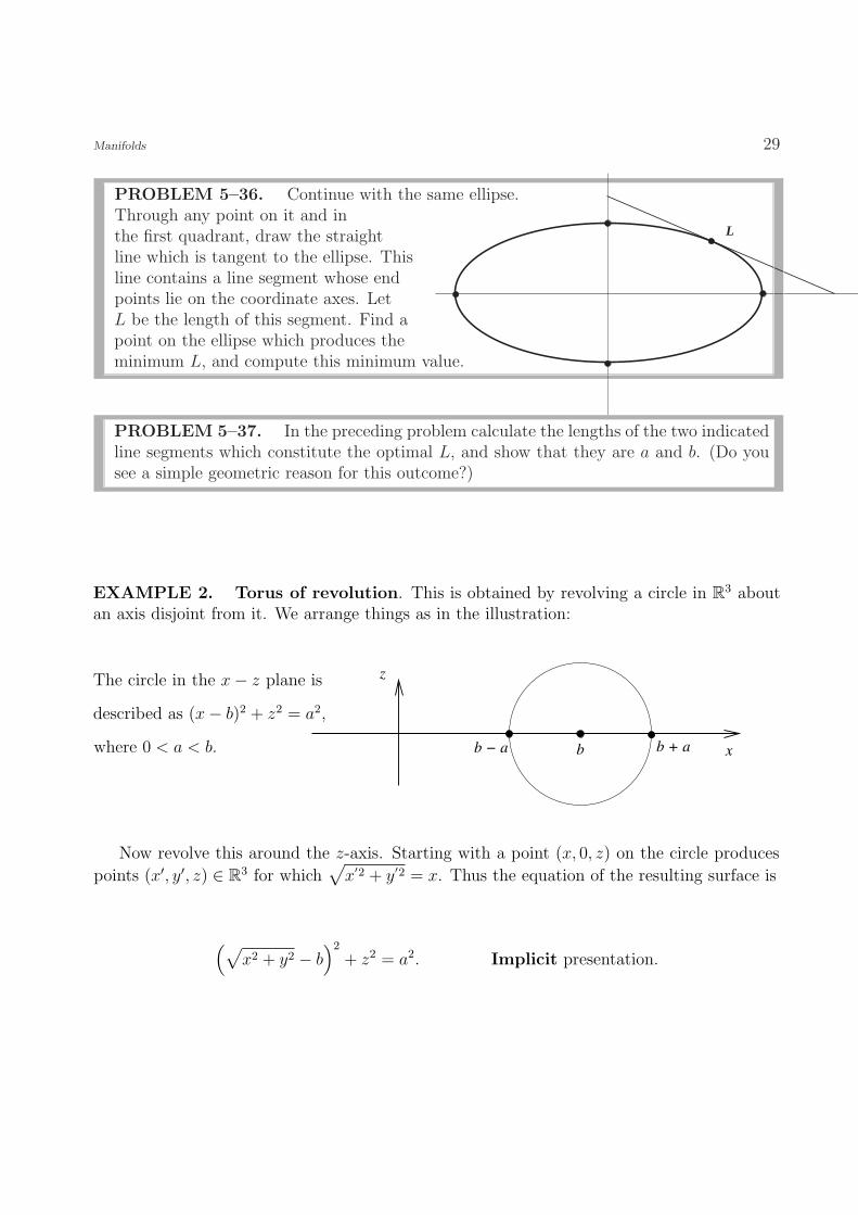
Manifolds 29

PROBLEM 5–36. Continue with the same ellipse.Through any point on it and inthe first quadrant, draw the straightline which is tangent to the ellipse. Thisline contains a line segment whose endpoints lie on the coordinate axes. Let

L

L be the length of this segment. Find apoint on the ellipse which produces theminimum L, and compute this minimum value.

PROBLEM 5–37. In the preceding problem calculate the lengths of the two indicatedline segments which constitute the optimal L, and show that they are a and b. (Do yousee a simple geometric reason for this outcome?)

EXAMPLE 2. Torus of revolution. This is obtained by revolving a circle in R3 aboutan axis disjoint from it. We arrange things as in the illustration:

The circle in the x− z plane is

described as (x− b)2 + z2 = a2,

b b + ab − a x

z

where 0 < a < b.

Now revolve this around the z-axis. Starting with a point (x, 0, z) on the circle produces

points (x′, y′, z) ∈ R3 for which√

x′2 + y′2 = x. Thus the equation of the resulting surface is

(√x2 + y2 − b

)2

+ z2 = a2. Implicit presentation.

30 Chapter 5

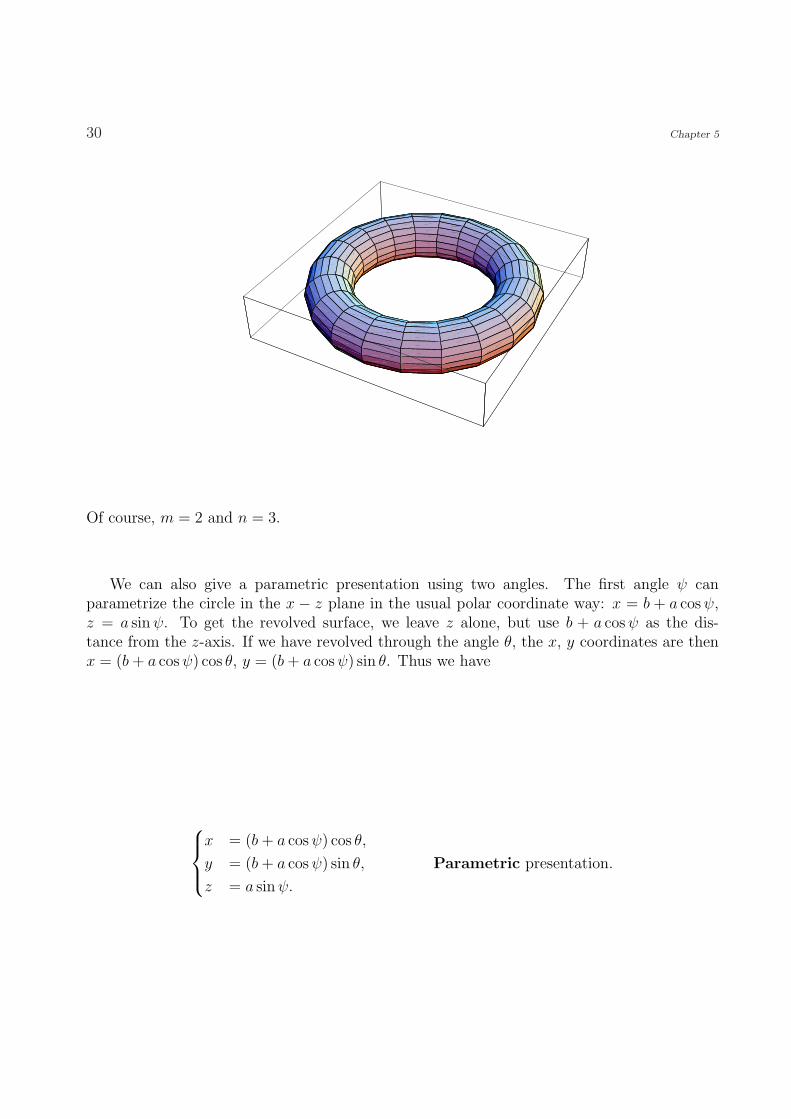
Of course, m = 2 and n = 3.

We can also give a parametric presentation using two angles. The first angle ψ canparametrize the circle in the x − z plane in the usual polar coordinate way: x = b + a cos ψ,z = a sin ψ. To get the revolved surface, we leave z alone, but use b + a cos ψ as the dis-tance from the z-axis. If we have revolved through the angle θ, the x, y coordinates are thenx = (b + a cos ψ) cos θ, y = (b + a cos ψ) sin θ. Thus we have

x = (b + a cos ψ) cos θ,

y = (b + a cos ψ) sin θ, Parametric presentation.

z = a sin ψ.

Manifolds 31

PROBLEM 5–38. Consider the given implicit presentation of the torus of revolution.The point (b + a, 0, 0) lies on this torus. Show that near this point the torus has theexplicit presentation

x =

√(b +

√a2 − z2

)2

− y2.

Show that the maximal region in the y− z plane for which this representation is valid hasthe shape:

(0, ) α

γ( , 0 )

semicircle

β( , 0 ) (0, 0)

What are α, β, and γ?

In a certain sense this torus of revolution can be thought of as the Cartesian product of twocircles, as two independent periodic coordinates ψ, θ are used in its presentation. However, itis not really a Cartesian product. There does exist a very interesting surface, a 2-dimensionalmanifold, which is actually the Cartesian product of two circles. As each circle is contained inR2, the Cartesian product we are going to exhibit is contained in R2×R2 = R4. This manifoldis often called a flat torus:

EXAMPLE 3. Just as R4 is the Cartesian product R2×R2 of two planes, this 2-dimensionalmanifold M is literally the Cartesian product of two circles:

M = {(x1, x2, x3, x4) | x21 + x2

2 = 1, x23 + x2

4 = 1}. Implicit presentation.

We can use the polar coordinates for the two unit circles to write the points of M in theform

x1 = cos θ1,

x2 = sin θ1, Parametric

x3 = cos θ2, presentation.

x4 = sin θ2.

32 Chapter 5

In a very definite sense to be explained later, this manifold is flat , unlike the torus of revolution.At any fixed point x ∈ M , we can find two linearly independent vectors orthogonal to M ,

using the implicit presentation; and two linearly independent vectors tangent to M , using theparametric presentation. Namely, orthogonal vectors can be found by using the gradients ofthe two defining functions:

(x1, x2, 0, 0) and (0, 0, x3, x4).

And tangent vectors can be found by using the partial derivatives ∂x/∂θi of the parametriza-tions:

(− sin θ1, cos θ1, 0, 0) and (0, 0,− sin θ2, cos θ2).

Thus we can split R4 into the 2-dimensional space orthogonal to M at x plus the 2-dimensionalspace tangent to M at x. We have just found the relevant orthonormal sequence:

(x1, x2, 0, 0)(0, 0, x3, x4)

}orthogonal to M,

(−x2, x1, 0, 0)(0, 0,−x4, x3)

}tangent to M.

Incidentally, we draw no pictures of the flat torus. It cannot be located in R3, whereas thetorus of revolution is a hypermanifold in R3. Thus it gives us an interesting example of a2-dimensional manifold in R4 which is not a hypersurface in R3.

These two manifolds are “topologically” indistinguishable. Without pausing to define theadjective, we go ahead and display a function

flat torusf−→ torus of revolution

in a rather obvious fashion. Namely,

f(x1, x2, x3, x4) =((b + ax3)x1, (b + ax3)x2, ax4

).

PROBLEM 5–39. Prove that f is a continuous bijection of the flat torus onto thetorus of revolution. Prove that its inverse is given as

f−1(x, y, z) =

(x√

x2 + y2,

y√x2 + y2

,

√x2 + y2 − b

a,

z

a

)

and that f−1 is also continuous.

Manifolds 33

Thus this function f provides a one-to-one correspondence between the points of these two tori,with the property that f and f−1 are both continuous. More than that, f and f−1 are bothinfinitely differentiable. Thus the flat torus and the “round” torus cannot be distinguished inthe sense of manifolds.

However, these tori are quite different geometrically . The round one is really a curvedsurface, and the surface appears quite different at different points. However, though we are asyet not equipped to define the adjective “flat,” it is rather clear that all points of the flat toruslook alike from a geometric perspective. Thus the two tori are distinct geometric objects.

PROBLEM 5–40. Prove that at any point of the torus of revolution the vectors

(− sin ψ cos θ, − sin ψ sin θ, cos ψ),

(− sin θ, cos θ, 0),

(cos ψ cos θ, cos ψ sin θ, sin ψ),

form an orthonormal basis of R3, the first two being tangent to the torus and the thirdorthogonal to the torus.