NBER WORKING PAPER SERIES

HISTORICAL PERSPECTIVESON THE MONETARY

TRANSMISSION MECHANISM

Jeffrey A. Miron

Christina D. Romer

David N. Well

Working Paper No. 4326

NATIONAL BUREAU OF ECONOMIC RESEARCH1050 Massachusetts Avenue

Cambridge, MA 02138April 1993

We are grateful to Ben Bemanke, Charles Calomiris, Philip Jefferson, GregoryMankiw, David Romer, Anna Schwartz and David Wilcox for helpfulcomments on earlier drafts of this paper. We are indebted to Matthew Jonesfor excellent research assistance. This paper is part of NBER's researchprogmm in Monetary Economics. Any opinions expressed are those of theauthors and not those of the National Bureau of Economic Research.

NBER Working Paper #4326April 1993

HISTORICAL PERSPECTIVESON THE MONETARY

TRANS MISS ION MECHANISM

ABSTRACT

This paper examines changes over time in the importance of the lending

channel in the transmission of monetary shocks to the real economy. We first

use a simple extension of the Bernanke-Blinder model to isolate the observable

factors that affect the strength of the lending channel. We then show that

based on changes in the stnicture of banks assets, reserve requirements, and the

composition of external firm finance, the lending channel should have been

stronger before 1929 than during the post-World War II period, especially the

first half of this period. Finally, we demonstrate that conventional indicators

of the importance of the lending channel, such as the spread between the loan

rate and the bond rate and the correlation between loans and output, do not

show the predicted decline in the importance of lending over time. From this

we conclude that either the traditional indicators are not useful measures of the

strength of the lending channel or that the lending channel has not been

quantitatively important in any era.

Jeffrey A. Miron Christina D. RomerDepartment of Economics Department of Economics270 Bay State Road University of CaliforniaBoston University Berkeley, CA 94720Boston, MA 02215 and NBERand NBER

David N. WeilDepartment of EconomicsBrown UniversityProvidence, RI 02912and NBER

1

1 IntroductionIn recent years, macroeconomists have devoted renewed attention tounderstanding the monetary transmission mechanism. According tothe standard "money" view, an open market sale of bonds by thecentral bank forces up interest rates because bond holders must becompensated with higher interest income for holding a less liquidcombination of assets. Although textbook presentations of this viewoften assume that banks are involved in the transmission of the openmarket sale, the presence of banks, and particularly bank loans, is inno way necessary.

The alternative "lending" view of the monetary transmission mech-anism assumes that bank loans are a special form of external finance.Banks do not regard loans and bonds as perfect substitutes on theasset side of their balance sheets, and firms do not regard bank loansas equivalent to other sources of funds on the liability side of theirbalance sheets. Since banks faced with a loss of reserves prefer toreduce the interest bearing component of their portfolio partly vialoans and partly via securities, and since firms do not view securitiesas perfect substitutes for bank loans, the interest rate on loans mustincrease relative to that on securities. This increase in the "spread"reflects an additional contractionary effect of restrictive monetarypolicy that is absent in the pure money view of the transmissionmechanism.

This paper provides historical perspective on the monetary trans-mission mechanism. Several recent papers attempt to determinewhether the special nature of bank lending impinges on the monetarytransmission mechanism (Bernanke (1983), Caiomiris and Hubbard(1989), Bordo, Rappaport and Schwartz (1991), Kashyap, Stein andWilcox (1993), Romer and Romer (1990), Hall and Thomson (1993)),and a number of these examine the transmission mechanism in par-ticular historical episodes (Calomiris and Hubbard (1989), Bordo,Rappaport and Schwartz (1991), Bernanke (1983)). None of thesepapers, however, explores changes in the nature of the transmissionmechanism over time. In this paper we examine directly the changes

2

in financial market institutions over the last one hundred years, andwe show how these changes can be used to assess the importance ofthe lending channel of monetary transmission.

Section 2 presents the basic analytical framework. We use theBernanke and Blinder (1988) model of the monetary transmissionmechanism to show under what conditions the response of the econ-omy to a monetary contraction should be especially sensitive to thepresence of a lending channel. Each of the conditions we identify canbe examined in the data over long historical periods. We can there-fore determine whether the lending channel appears to be impor-tant in periods when theory combined with evidence on the financialstructure suggests it should be important.

Section 3 of the paper examines empirically those features of bankand firm balance sheets that our theoretical discussion suggests aremost relevant to the quantitative importance of the lending chan-nel. In particular we document how factors such as the structureof reserve requirements and the composition of external firm financehave changed over time. Our analysis shows that the lending chan-nel should have played a much greater role in the pre-1929 era thanduring the post-World War II period, especially the early part of thisperiod.

In Section 4 we present new evidence on the lending channelby determining whether measures of the importance of bank lend-ing behave differently across periods characterized by differences inthose factors that our theoretical discussion suggests determine thestrength of the lending channel. The measures we consider are thespread between the interest rate on bank loans and the interest rateon commercial paper, the ratio of bank loans to other sources ofcredit (the "mix"), and the relation between bank loans and outputafter monetary contractions and in more ordinary times. We findlittle evidence that these measures of the importance of the lendingchannel change across time periods in the ways implied by changesin financial structure and institutions.

Section 5 concludes the paper. The evidence we present can be

3

interpreted in at least two ways. On the one hand, it may indicatethat traditional indicators of the importance of the lending channelare not useful. On the other hand, it may indicate that the lendingchannel has not been particularly important in any sample period.Our analysis does not rule decisively on which of these two explana-tions is correct. However, since the most obvious indicators of thelending channel fail to provide consistent evidence of its importancewe believe proponents of this view are likely to have a difficult timeproviding a compelling case for its empirical relevance.

2 Framework for AnalysisWe begin by laying out a model of the monetary transmission mech-auism that considers the relative importance of different financingchannels. The model is a modified version of the one presented inBernanke and Blinder (1988). We use the model to highlight the roleof various institutional features in determining the importance of thelending channel.

2.1 The Model

We begin by considering the more familiar model in which loans playno role. The only assets are money, in, and bonds, 6. Our notationis that small letters signify quantities, capital letters signify func-tions, subscripts signify derivatives, and superscripts signify subsetsof quantities (e.g., b is bonds while bb is bonds held by banks). Sincethe price level and the inflation rate are held fixed throughout, wenormalize them to 1 and 0, respectively. All variables are thereforein real terms.

The demand for money depends on output, y, and the bond in-terest rate, i,(1) m=D(i,y).As in the standard IS curve, output depends negatively on the inter-

4

est rate,(2) y=Y(i).Differentiating (1) and (2) yields

13\dy _____dmD1+DYi

Equation (3) shows the effect money on output when only the moneychannel is operational.

Theories of the lending channel begin by recognizing the existenceof another asset, loans, 1. The banking sector's balance sheet is then

(4) m=bb+1+r,

where r is reserves and bb is net holdings of bonds by banks. Notethat we treat time deposits and CDs as bank-issued bonds, whichare subtracted from bank holdings of bonds in calculating bb. Allmoney is held in the form of deposits, which are liabilities of banks.Non-bank holdings of nominally denominated assets, w, are given by

(5)

where b is net bond holdings of the non-bank public. Note thatwe include both firms and households in the non-bank sector. Thisformulation assumes that in the short run the stock of nominallydenominated assets held by the non-bank sector is fixed.

Introducing a third asset requires introducing a second interestrate. Rather than including the interest rate on loans directly, weintroduce the difference between the loan interest rate and the bondinterest rate, 8, which affects investment demand. Thus (2) becomes

(6) y =

where ' < 0 and Y5 < 0. The demand for loans by the non-bankpublic is(7) 1 =

5

where L5 < 0. We discuss the signs of L1 and L below.Banks hold deposits as liabilities and loans and reserves as assets.

Combining the models of Romer and Romer (1990) and Bernankeand Blinder (1988), we allow banks to hold bonds as either assets orliabilities, with time deposits and CDs defined as bank issued bonds.We define b6 as banks' net holdings of bonds. As discussed by Romerand Romer, bond issues by banks may or may not require significantreserve holdings. We assume that if reserve requirements are imposedon bond issue, then banks will not both hold and issue bonds, exceptfor small quantities of bonds held for liquidity purposes. Thus thereserve requirement holds on the net issue of bonds.

We take the fraction of bank deposits held as reserves againstdemand deposits to be constant at some level r1 that can be thoughtof as required or desired reserves. Reserves against bond issues aretaken to be constant at rate r2. Banks choose the fraction of non-reserve assets held in the form of loans as a function of the loan-bondinterest differential,

(8) l+1bb A=A(S),where A5 > 0.1 If A is less than one, banks holds bonds on net. If Ais.greater than one, banks issue bonds on net.

In the case where banks are net holders of bonds, the supply ofloans is(9) 1 = A()(1 — ri)m.In the case where banks are net issuers of bonds, the supply of loans

10 1- ( A(6)(1-ri)-1+(A()-1)r2

Note that if the reserve requirement on bond issues is zero, thenequations (9) and (10) are the same. Thus in the rest of this section,we assume that reserves are held on net bond issues and then discussthe cases where no such reserves are held by setting r2 to zero.

6

Equating the supply and demand for loans yields

/ A(6)(1—ri) \(11) L(5,z,y)= l+(A(5)_l)T2)m.Equations (1), (6), and (11) determine the levels of y, i, and 5 giventhe level of m. Totally differentiating the three equations, the effectof a change in the money supply on output is

(12)dydm

(A5 ( l—72 \ L5"1 (YI\ (L1'\ (D,A l+(A-l)r2)

-1) Y5) + 1)

(As ( 1 — r2 ' — Lö'\ (D + DY + (L1D — LD,kA1+(A—l)r2) Y5 I

This equation shows the effects of an open market sale that reducesm and raises either bb or b, holding w constant, when both a lendingchannel and a money channel are operational.

2.2 Simplifying AssumptionsWe now add further assumptions to simplify expression (12). Webegin with the interest elasticities of the non-bank public's demandsfor different assets. Starting from the non-bank sector's holdingsof nominally denominated assets, we have the usual adding up con-straint(13)

where BP(.) is the non-bank public's demand for bonds. Dividing bythe total amount of deposits and re-arranging gives

(14) m im bmThis equation relates the percentage change in deposits in response toan interest rate increase to the percentage changes in loan and bond

7

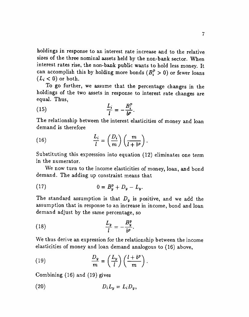
holdings in response to an interest rate increase and to the relativesizes of the three nominal assets held by the non-bank sector. Wheninterest rates rise, the non-bank public wants to hold less money. Itcan accomplish this by holding more bonds (B' > 0) or fewer loans(L <0) or both.

To go further, we assume that the percentage changes in theholdings of the two assets in response to interest rate changes areequal. Thus,

r. pP(15'l —\1

1 bP

The relationship between the interest elasticities of money and loandemand is therefore

16m

(1 m)l+bP

Substituting this expression into equation (12) eliminates one termin the numerator.

We now turn to the income elasticities of money, loan, and bonddemand. The adding up constraint means that

(17) 0=B+D—L.The standard assumption is that D is positive, and we add theassumption that in response to an increase in income, bond and loandemand adjust by the same percentage, so

L B18 =1 bP

We thus derive an expression for the relationship between the incomeelasticities of money and loan, demand analogous to (16) above,

(19) = (L (1 + bP)m \1J\ mCombining (16) and (19) gives

(20) DL =

8

which eliminates one term in the denominator of the expression fordy/dm derived above.2

Incorporating these assumptions about elasticities, the derivativeof output with respect to money becomes

(A5( l-T2 \ L5\(Y (b'+l-m'(D1dy k,1+—1)r2) i)y5) b+ldm (As( 1-T2 Ls'(D+DY1k l+—1)r2)

(21)This expression shows the effects of money on output when a lend-ing channel is operational, assuming our simplifying assumptions areapproximately correct. Several comments about this expression arein order.

The conditions for a lending channel to be operational are thatA5 < , L5 > —, and Y5 < 0. If any of these conditions fails tohold, then (21) collapses to (3). The first of these conditions statesthat banks do not regard loans and bonds as perfect substitutes intheir portfolios; the second states that firms do not regard loans andbonds as perfect substitutes in their portfolios; and the third statesthat firms' investment decisions depend on both the loan and bondinterest rates.

The condition for money to have a greater effect on output whenthe lending channel is operational (i.e., the condition for the expres-sion in (21) to exceed the expression in (3)) is that

(22) b'+l—m>O.Since this term can be positive or negative, the lending channel canexacerbate or moderate the money channel's effect on output. Fromthe bank's baiance sheet,

(23) l—m= _bb_r.So, the condition for the lending channel to exacerbate the effect ofmoney on output is that

(24) bb+r<b.

9

We assume in what follows that this condition is satisfied.

2.3 The Determinants of dy/dm

Having laid out the basic model, we now consider how observablefeatures of the institutional and financial structure of the economyare likely to affect the impact of money on output, assuming a lendingchannel is operational. Our discussion focusses on two broad areasthe structure of bank balance sheets and the structure of firm finance.

The first factor likely to determine the magnitude of money'seffect on output is the structure of bank assets. Assuming that con-dition (24) is satisfied, dy/dm is largest when A5[A is small, thatis, when banks do not adjust the fraction of their assets made up ofloans in response to a change in the loan-bond differential. Uiderthe assumption that A5 does not vary significantly with A, this wouldimply that dy/din is increasing in the fraction of their portfolios thatbanks hold in loans.

More generally, the effect of changes in A on As/A depends on theunderlying model of bank portfolio preferences. One case where onecan determine the magnitude of A5/A is when there is a significantreserve requirement on the issue of bonds by banks and A (the frac-tion of the banks portfolio made up of loans) is near one. In this casebanks are likely to be at a corner, in which the the marginal cost ofone less loan (the interest rate on holding bonds, which is the oppor-tunity cost of making loans) could be much less than the marginalcost of one more loan (that is, the bond interest rate adjusted forthe cost of holding reserves against bond issue). In such a case, theelasticity of the portfolio share with respect to the loan-bond differ-ential is likely to be near zero and thus, other factors held constant,dy/dm should be large.

The second factor affecting the size of dy/dm is the structure offirm finance. Expression (21) indicates that the fraction of firms'capital coming from loans relative to bonds likely affects the magni-tude of the lending channel by changing the semi-elasticity of loandemand with respect to the loan-bond differential, L5/l. As loans

10

increase as a fraction of firm finance, we expect L5/1 to fall, thusincreasing dy/dm.

A third factor in the size of dy/dm is the relative size of thesensitivities of investment to the bond interest rate and to the loan-bond differential. Holding Y constant, an increase in ratio of Y5 toV, raises the value of dy/dm. This ratio will be affected by both thedifferent fractions of investment being financed at the loan and bondrates and by the potential for substitution between the two. If, forexample, "small" firms invest using loans while "large" firms investusing bonds, if there is no substitution between the two sources offinancing, and if the two size firms have the same interest elasticityof investment, then Y5/Y will just equal the fraction of firms that issmall. Differences in the interest elasticities of investment betweenlarge and small firms will affect the ratio of Y5 to Y. If small firmsare more interest sensitive than are large firms, dy/dm will be bigger.Finally, if firms are able to substitute between loans and bonds intheir financing, this will reduce Y5 and thus reduce dy/dm.

3 Changes in Financial StructureAccording to the model presented in Section 2, changes in the finan-cial structure of the economy have important implications for theimportance of the lending channel in the transmission of monetaryshocks. Therefore, to see if the importance of the lending channel islikely to have changed over time in the United States, we examineevidence on how various aspects of financial structure have changedbetween 1900 and 1988. In particular, we look at structural changesin the balance sheets of banks and firms.

The major finding of this analysis of institutions is that the lend-ing channel of the monetary transmission mechanism should havebeen stronger before 1929 than after 1945, particularly in the firsttwo decades after 1945. We find that important changes in financialstructure occurred between the pre-Depression and post-World WarII eras and that, at least up through 1970, essentially all of these

11

changes imply a weakening of the lending channel. After 1970 theevidence is more complicated, with some changes further weakeningthe lending channel and others potentially strengthening it.

3.1 Banks

3.1.1 Assets

Annual data on bank balance sheets for 1896 to the present are avail-

able from the Federal Reserve. These data reflect a major effort bythe Federal Reserve to adjust the historical statistics for the prewarera (from the Comptroller of the Currency) to be as consistent aspossible with postwar statistics. This adjustment mainly involvesinflating the data for non-national banks to compensate for under-reporting by state banks in the period before 1938. In this sectionwe use the version of the Federal Reserve data corresponding to allcommercial banks.3

Figure 1 shows the ratio of total bank loans less real estate loa.nsto total interest-bearing bank assets for 1896 to 1988. This ratiodeclined slowly over the first three decades of the 20th century, from72 percent in 1896 to 60 percent in 1929. It then fell dramaticallyduring the Great Depression and World War II, reaching 17 percentin 1945. Between 1945 and 1970 it rose steadily, reaching 27 percentin 1950, 46 percent in 1960, and 53 percent in 1970. Since 1970non-real estate loans as a fraction of total bank assets have hoveredaround 52 percent.

Mirroring this fall over time in the loan ratio is a rise over timein the fraction of bank assets accounted for by government securi-ties. Government securities accounted for between 5 and 7 percentof interest-bearing bank assets during most of the pre-Worid War Iera. After the war this number was higher; in 1929, for example,government securities accounted for 10 percent of total assets. Dur-ing World War II banks increased their holdings of U.S. governmentsecurities by a factor of four. This came on top of a threefold increasebetween 1929 and 1936. As a result, government securities accounted

12

for 73 percent of total interest-bearing assets in 1945. Bank's hold-ings of government securities then fell steadily in the first two decadesof the postwar era as loans rose. However, as the behavior of the loanratio suggests, the fraction of bank assets accounted for by govern-ment securities never returned its pre-Worid War I level; in 1988government securities were still 14 percent of total bank assets.

This pattern suggests that loans were, on average, a substan-tially larger fraction of total interest-bearing bank assets in the pre-Depression era than in the post-World War II period. Even at thepostwar peak, the fraction of bank assets accounted for by non-realestate loans was more than 10 percentage points smaller than theaverage fraction in the pre-1929 period. In terms of the model givenin Section 2, holding other factors constant, this change implies thatthe lending channel was substantially more important before 1929than after 1945.

The implications of the low loan holdings during the period 1929-1944 are harder to determine because the period is short and dom-inated by the Great Depression. The plummeting of the fraction ofbank assets accounted for by loans between 1929 and 1936 almostsurely reflects the tremendous fall in output, rather than some in-stantaneous change in the importance of the lending channel. Thus,a reasonable view is that the lending channel was as important duringthe declining phase of the Depression as it was in the three decadesbefore 1929. On the other hand, after the recovery was firmly underway, it seems possible that the continued low loan ratios, includingthe additional declines associated with World War II, imply that thelending channel was considerably weaker in the late 1930s and early1940s than previously. Once banks had switched so thoroughly outof loans and into other assets, a decline in reserves should have hadless effect on bank lending.

3.1.2 Liabilities.

The structure and level of reserve requirements has changed dramat-ically over time. Figure 2a shows the ratio of the reserve requirement

13

on time deposits to the reserve requirement on demand deposits overthe last century. Figure 2b shows the level of the reserve require-ment on time deposits. Construction of these figures is somewhatcomplicated due to changes in the definition of time deposits and tothe variation in state regulations before the founding of the FederalReserve in 1914. For the period before 1917, we analyze reserve re-quirements for national banks, as set by the National Banking Actof 1864 and various amendments. These figures are also complicatedby the fact that the definition of deposits was changed substantiallyby the Monetary Control Act of 1980.

Under the National Banking Act no distinction was drawn be-tween time deposits and demand deposits; there was a uniform re-serve requirement on all deposits. Thus, the ratio of the reserverequirement on time deposits to that on demand deposits for na-tional banks was one from 1874 until the founding of the FederalReserve. Effective in 1917, the Federal Reserve Act distinguishedbetween time and demand deposits, setting the ratio of the reserverequirements on the two at an initial level of roughly one to three.Though there was some variation in this ratio during the interwarand early postwar eras, it remained at roughly one to three untilthe mid-1960s. The relative size of the requirement on time depositswas lowered significantly in 1967, and the ratio hovered around 1/6through the 1970s. After 1980 the ratio rose to 1/4, but this changeis somewhat hard to interpret because of the change in the definitionof deposits.

The change in the ratio of reserve requirements on time and de-mand deposits in the postwar era is even more dramatic if one con-siders special time deposits rather than ordinary savings accounts.An important development of the 1960s was the advent of certificatesof deposit.6 While CDs had roughly the same reserve requirements assavings deposits in the late 1960s, in the 1970s their reserve require-ment fell from 3 percent to 1 percent. In 1980, under the MonetaryControl Act, the reserve requirement on CDs over a certain level wasset to zero. As a result of this change, banks in the late 1970s and

14

1980s had a way of raising funds that was free of reserve limitations.The level of the reserve requirement on time deposits follows al-

most the same pattern as the ratio of the reserve requirement on timedeposits to that on demand deposits. Under the National BankingAct the reserve requirement on time deposits was not only the sameas that on demand deposits, it was also very high (25%). With theadvent of the Federal Reserve, the reserve requirement on time de-posits fell dramatically (to 3%). This level rose somewhat duringthe Great Depression and the early postwar era (to between 5 and7.5%), before returning to 3% in 1967. Once again, if special timedeposits are considered rather than savings accounts, changes occuragain in 1975 and 1980 when the reserve requirement on CDs waslowered and then eliminated.

As mentioned above, the discussion of reserve requirements forthe pre-Worid War I era is complicated by the presence of statebanks that were subject to individual state reserve requirements.In the period before World War I there was substantial variationin state regulations. Before detailing the differences between stateand national bank regulations, it is important to note that nationalbanks account for a large fraction of total bank assets in the earlyperiod. National banks accounted for 42% of total bank asssets in1896 and 43% in 1910. Thus, nearly half of bank deposits in theprewar era certainly had equal reserve requirements on demand andtime deposits.

A systematic study of state reserve requirement legislation byRodkey (1934) indicates that most state banks had similar reserverequirements on demand and time deposits during the period be-fore the founding of the Federal Reserve. However, Rodkey listseleven states that passed legislation distinguishing between the dif-ferent types of deposits in the setting of reserve requirements. Thesestates were (in order of date of legislation) Maine, New Hampshire,Nebraska, Iowa, North Carolina, Oregon, Pennsylvania, Connecticut,Vermont, Utah, and Colorado. In most of these states, however, theratio of the reserve requirement on time deposits to that on demand

15

deposits was much closer to one than in the post-Federal Reserveperiod, and the level of reserve requirements on time deposits wassubstantial. For example, in the Pennsylvania statute passed in 1907,the reserve requirement on time deposits was 7.5% and that on de-mand deposits was 15%. In the Utah statute passed in 1911, thereserve requirement on time deposits was 10% and that on demanddeposits was 15%.

Those states that had similar reserve requirements on time de-posits and demand deposits typically set fairly high reserve require-ments. A study by Welidon (1909) of state regulations in 1909found that reserve requirements on time and demand deposits instate banks were usually between 15 and 25%. However Weildonfound that in 1909, 14 states had zero reserve requirements on bothtime and demand deposits. Since reserve requirements were becom-ing more common over time, the number of states with no reserverequirements was surely much larger in the 1870s and 1880s.

Given that the majority of state banks set equal and high reserverequirements on time and demand deposits in the pre-Federal Re-serve era, it is reasonable to conclude that the ratio of the reserverequirement on time deposits to that on demand deposits fell sub-stantially between the pre-1914 era and the. interwar and postwarperiods. Furthermore, within the post-World War II period, the ra-tio fell even more. The level of reserve requirements on time depositsalmost surely showed the same pattern.

To look directly at the importance of time deposits to bank bal-ance sheets, Figure 3a presents the ratio of time deposits to totalinterest-bearing assets of commercial banks.8 The relative size oftime deposits, though small, rose through the pre-Fed period andcontinued to rise through the onset of the Depression. The relativemagnitude of time deposits fell during World War II, but then roseswiftly during the post-War period, with time deposits (includingCDs) becoming the dominant liability of commercial banks in the1970's and 1980's.

The change in the structure of reserve requirements over time and

16

the corresponding rise in the importance of time deposits, suggestthat the lending channel should have been weakened between thepre-1914 and post-World War II periods. In the pre-Federai Reserveera, banks had little opportunity to raise funds to counteract a fallin reserves because all deposits were covered by the same reserverequirements. Thus, loans had to contract in response to a fall inreserves. In contrast, in the 1980s, banks could issue CDs which haveno reserve requirement. As a result, loans no longer needed to fall inresponse to a decline in reserves.

Figure 3b plots our summary measure of banks' portfolios, A,which is the ratio of loans to net interest bearing assets (loans plusnet bond holdings). During the period before the Great Depression,A remained near one, reflecting the fact that banks' net holdings ofbonds were near zero. During the first part of this period,.when therewere substantial reserve requirements on time deposits, we suspectthat banks were at a corner with respect to the fraction of their netassets made up of loans. More generally, the fact that A was sonear toone and showed so little variation suggests that banks were reluctantto change the composition of their portfolios in response, for example,to a change in the loan-bond differential. In such a case, accordingto. the model laid out above, the lending channel will be particularlypotent. Over the postwar period, A rose steadily, reflecting both anincrease in loans on the asset side and an increase in time depositsas liabilities. The effect of these changes in A on the importanceof the lending channel in the post-War era are ambiguous. On theone hand, the high values of A in the latter half of the period mightsuggest that As/A was small and the lending channel important. Onthe other hand, the large range of values over which A varied mightsuggest that banks were not reluctant to adjust their portfolios, andthus that that the lending channel was not important.

3.2 Firms

According to the model given in Section 2, changes in the compo-sition of firm finance and the relative size of large and small firms

17

over time would cause the importance of the lending channel of mon-etary transmission to change as well. If firms use fewer loans relativeto other liabilities to finance investment, this should decrease theimportance of the lending channel. This is true because a lower em-phasis on loan finance means that firms are less sensitive to changesin the loan-bond interest differential. Since small firms are likely tobe more constrained in their alternatives to bank credit, a fall in theproportion of firms that are small implies that the lending channelis likely to have become less important as well.9

3.2.1 Aggregate Behavior.

Perhaps the simplest measure of the importance of bank loans in thefinancing of firms is the ratio of total bank loans (less real estateloans) to the capital stock. This measure provides an indication ofwhether bank loans grew faster, slower, or at just the same rate asthe capital which such loans are designed to finance. The data ontotal non-real estate bank loans are taken from the balance sheet forall commercial banks described above. The capital stock series usedshows the net stock of fixed, nonresidential private capital.'O Sincethe loan series is in current dollars, we use the current-cost valuationcapital stock series as well. Because the capital stock series onlystarts in 1925, we can only look at the ratio starting at the end ofthe pre-Depression era.

Figure 4 shows the ratio of total non-real estate bank loans to thecapital stock. As can be seen, in the late 1920s this ratio was between26 and 29 percent. During the Depression, the ratio plummeted asloans fell dramatically. The ratio remained below 20 percent until1960. During the early 1970s, it reached levels close to the typicalvalue in the late 1920s. In the late 1970s and early 1980s, the ratioof loans to the capital stock fell again, to values close to 20 percent.This picture certainly suggests that loans were a more importantsource of firm finance at the end of the pre-Depression era than inthe postwar era. However, what happened during the early years ofthe 20th century cannot be discerned.

18

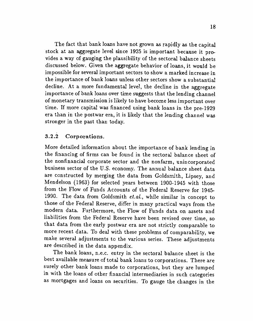
The fact that bank loans have not grown as rapidly as the capitalstock at an aggregate level since 1925 is important because it pro-vides a way of gauging the plausibility of the sectoral balance sheetsdiscussed below. Given the aggregate behavior of loans, it would beimpossible for several important sectors to show a marked increase inthe importance of bank loans unless other sectors show a substantialdecline. At a more fundamental level, the decline in the aggregateimportance of bank loans over time suggests that the lending channelof monetary transmission is likely to have become less important overtime. If more capital was financed using bank loans in the pre-1929era than in the postwar era, it is likely that the lending channel wasstronger in the past than today.

3.2.2 Corporations.

More detailed information about the importance of bank lending inthe financing of firms can be found in the sectoral balance sheet ofthe nonfinancial corporate sector and the nonfarm, unincorporatedbusiness sector of the U.S. economy. The annual balance sheet dataare constructed by merging the data from Goldsmith, Lipsey, andMendelson (1963) for selected years between 1900-1945 with thosefrom the Flow of Funds Accounts of the Federal Reserve for 1945-1990. The data from Goldsmith et.al., while similar in concept tothose of the Federal Reserve, differ in many practical ways from themodern data. Furthermore, the Flow of Funds data on assets andliabilities from the Federal Reserve have been revised over time, sothat data from the early postwar era are not strictly comparable tomore recent data. To deal with these problems of comparability, wemake several adjustments to the various series. These adjustmentsare described in the data appendix.

The bank loans, n.e.c. entry in the sectoral balance sheet is thebest available measure of total bank loans to corporations. There aresurely other bank loans made to corporations, but they are lumpedin with the loans of other financial intermediaries in such categoriesas mortgages and loans on securities. To gauge the changes in the

19

importance of bank loans, we compare bank loans to the sum oftotal liabilities of corporations, less trade debt and the market valueof corporate equities. While gross trade debt is typically included intotal liabilities, it is not a large net source of finance for the corporatesector because firms owe most of it to each other. Therefore, weexclude gross trade debt from total liabilities. Figure 5 shows theratio of bank loans n.e.c to total liabilities less trade debt plus equitiesfor nonfinancial corporations.

This graph shows that the loan ratio of corporations rose overthe course of the pre-Depression era, from 11 percent in 1900 to 14percent in 1922. By 1929, however, it had fallen back to 8 percentbecause of the explosion in the market value of corporate equities. Itthen fell further during the Depression, reaching 6 percent in 1933.The corporate loan ratio started the postwar era fairly high, reaching11 percent in 1947, but then dropped substantially in the 1950s.During the 1950s and 1960s, the ratio hovered around 7 percent.It then rose in the 1970s, but, with the exception of 1974, it didnot reach its pre-Depression peak value. Based on this graph, itappears that the loan ratio for corporations was noticeably higher inthe pre-Depression era than in the first two decades of the postwarera. After 1970, loans have increased in importance, but they arestill less important than in the first decades of the 1900s.

The decreased role of bank loans in the postwar era has varioussources. One widely cited change in corporate finance between thepre-WWI era and the interwar and postwar periods is the expansionof the commercial paper market (see, for example, Cargill, 1991, p.140 and Greef, 1938). However, even though the commercial papermarket expanded significantly, especially after 1960, it is still a verysmall fraction of total liabilities. Thus, it is not the main sourceof the decreased importance of loans. The more important changeis the expansion of corporate equities. Corporate equities increasedmuch faster between the pre-1929 and postwar eras than did loans ortotal liabilities (less trade debt). Indeed, the ratio of loans to totalliabilities (less trade debt) was roughly the same in the early 1900s

20

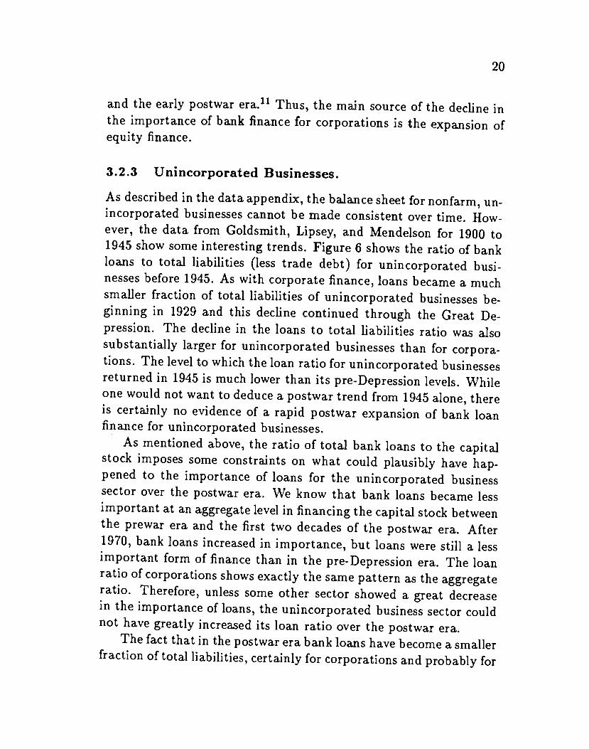
and the early postwar era.11 Thus, the main source of the decline inthe importance of bank finance for corporations is the expansion ofequity finance.

3.2.3 Unincorporated Businesses.

As described in the data appendix, the balance sheet fornonfarm, un-incorporated businesses cannot be made consistent over time. How-ever, the data from Goldsmith, Lipsey, and Mendelson for 1900 to1945 show some interesting trends. Figure 6 shows the ratio of bankloans to total liabilities (less trade debt) for unincorporated busi-nesses before 1945. As with corporate finance, loans became a muchsmaller fraction of total liabilities of unincorporated businesses be-ginning in 1929 and this decline continued through the Great De-pression. The decline in the loans to total liabilities ratio was alsosubstantially larger for unincorporated businesses than for corpora-tions. The level to which the loan ratio for unincorporated businessesreturned in 1945 is much lower than its pre-Depression levels. Whileone would not want to deduce a postwar trend from 1945 alone, thereis certainly no evidence of a rapid postwar expansion of bank loanfinance for unincorporated businesses.

As mentioned above, the ratio of total bank loans to the capitalstock imposes some constraints on what could plausibly have hap-pened to the importance of loans for the unincorporated businesssector over the postwar era. We know that bank loans became lessimportant at an aggregate level in financing thecapital stock betweenthe prewar era and the first two decades of the postwar era. After1970, bank loans increased in importance, but loans were still a lessimportant form of finance than in the pre-Depression era. The loanratio of corporations shows exactly the same pattern as the aggregateratio. Therefore, unless some other sector showed a great decreasein the importance of loans, the unincorporated business sector couldnot have greatly increased its loan ratio over the postwar era.

The fact that in the postwar era bank loans have become a smallerfraction of total liabilities, certainly for corporations and probably for

21

unincorporated businesses, makes it likely that the lending channelof the transmission mechanism has weakened over time. In terms ofour model, if there are more substitutes for bank loans in the postwarera than in the pre-1929 era, then the sensitivity of investment to theloan-bond spread should have diminished. This in turn implies thatthe relative importance of the lending channel should have declinedas well.

The fact that loans have become a more important source of firmfinance over the course of the postwar era suggests that the relativeimportance of the lending channel may not have been constant be-tween 1945 and 1990. Indeed, judging just from the facts about firmfinance, it appears quite likely that the lending channel becamemoreimportant after 1970 than it was in the 1950s and 1960s, though notas important as in the pre-Depression era.

3.2.4 Relative Size of Corporations and UnincorporatedBusinesses.

While the classification of particular liabilities for unincorporatedbusinesses cannot be made consistent over time, the data for total II-abilities and equities do appear to be comparable across time periods.Therefore, it is possible to use this information to gauge the relativesize of the corporate and unincorporated sectors.12 Since corpora-tions are typically much larger than unincorporated businesses, thiscomparison can give some indication of changes in the distributionof large and small firms over time. Figure 7 graphs the ratio of totalliabilities (less gross trade debt) of unincorporated businesses to thesum of total liabilities (again, less gross trade debt) of corporationsand corporate equities.

Judging from this measure, the corporate sector grew more rapidlythan the unincorporated sector between 1900 and 1945; the ratio oftotal liabilities of unincorporated businesses to total liabilities plusequities of corporations fell steadily over this period. In the earlypostwar era, the ratio hovered at roughly the same level as in 1929.After 1970, this ratio rose substantially, reflecting the greater growth

22

of total liabilities for unincorporated businesses.If this ratio truly reflects the relative size of the two sectors,

and the lending channel is more important the larger is the bank-dependent unincorporated sector, then the fall in the ratio between1900 and 1945 suggests that the lending channel of monetary trans.mission was weakening over this period. It then remained at its 1929level during the early postwar era. The subsequent rise in the rel-ative size of the two sectors suggests that the lending channel hasbecome more important again in the last two decades.

3.3 Summary

Taken together, the various changes in the structure of financial in-stitutions suggest that the lending channel should have decreased inimportance between the pre-1929 and the post-1945 eras. Roth thestructure of bank balance sheets and the structure of firm balancesheets suggests that loans were more important before the GreatDepression than after. Within the pre-Depression era, the differenti-ation of reserve requirements on time deposits and demand depositsand the large decline in the level of reserve requirements on timedeposits at the time of the founding of the Federal Reserve suggeststhat the lending channel should have been stronger before 1914 thanafter.

Within the postwar era, the fact that bank loans have becomea larger fraction of total bank assets and total firm liabilities af-ter 1970 than in the first two decades of the postwar era suggeststhat the lending channel may have been increasing in importance.The relative importance of unincorporated (and presumably bank-dependent) businesses also rose in the second half of the post-WorldWar II era, again suggesting an increased importance of the lend-ing channel. However, the ratio of the reserve requirement on timedeposits to that on demand deposits and the level of reserve require-ments on time deposits fell in the late postwar era, and time depositsand CDs rose to become the dominant liability of commercial banksover the postwar period. These factors would tend to lessen the

23

importance of the lending channel. Thus, while it is clear that thelending channel should have weakened between the pre-Depressionera and early postwar eras, the relative strength of the lending chan-nel in the early and late postwar eras is ambiguous.

4 Historical Evidence on the Lending Chan-nel

In this section we examine the behavior since the late 19th centuryof various indicators of the strength of the lending channel. In par-ticular, we look at the spread between the loan and bond rates, themix of credit market instruments between loans and commercial pa-per, and the correlation between output and lending. The analysis ofSection 2 and previous analytical work suggest that these measuresshould behave differently after monetary contractions than in moreordinary times if the lending channel is important. Since the institu-tional analysis of Section 3 suggests that the strength of the lendingchannel should have declined over time, our hypothesis is that theresponse of these variables to monetary shocks should have declinedas well. If they have not, this could either be evidence that thesemeasures of the strength of the lending channel are not very good,or evidence that the lending channel has not been important in anyera.

Since the response of these variables to monetary contractionsis the measure of the strenght of the lending channel, identifyingmonetary contractions is an important step in the analysis. Themonetary contractions that we consider consist of three pre..FederalReserve financial panics (1890:8, 1893:5, and 1907:10); four interwarcontractions consisting of Friedman and Schwartz's (1963) three cru-cial experiments plus the bank holiday (1920:1, 1931:10, 1933:2, and1937:1); and seven post-Word War II episodes identified by Romerand Romer (1989, 1992) as anti-inflation interventions by the Fed-eral Reserve (1947:10, 1955:9, 1968:12, 1974:4, 1978:8, 1979:10, and1988:12). The extent to which each of these episodes constitutes

24

an exogenous monetary contraction has been debated at length else-where (Friedman (1989), Schwartz (1989), Hoover and Perez (1992),Dotsey and Reid (1992)); we do not repeat that discussion here.

4.1 The Spread

According to the model presented above, one key indicator of thestrength of the lending channel is 5, the spread between loan ratesand bond rates. In response to a monetary contraction, the spreadshould increase as banks contract loans, and thus force firms to usebonds as an imperfect, alternate source of finance. Using the frame-work in Section 2, and incorporating the simplifying assumptionsused there, the response of the spread to a change in the moneystock is

(b7'+1—m\ (1dS — — bP+1 )

(A( 1—r2 '\ L51+(—1)r2) I

The factors that imply a large response of the spread to money are asubset of those that lead to a large value of dy/dm in equation (21)above. The less willing are banks and firms to substitute betweenloans and bonds in response to changes in the spread, the larger willbe the effect of money on the spread. Similarly, in the case wherebanks are net issuers of bonds, the larger is the reserve requirementon CD's and time deposits, the larger will be the effect of money onthe spread. On the other hand, the sensitivities of investment to thebond interest rate and to the spread, which affect the size of dy/dm,do not affect the sensitivity of the spread to money shocks.

4.1.1 Data

Figure 8 presents a measure of the spread for the period 1890-1991.The loan rate series is the time loan rate on six-month time loansfor the period 1890-1918, the rate charged on customer loans bybanks in principal cites for the period 1919-1927, the rate charged

25

on commercial ioans by banks in principal cities for the period 1928-1939, and the prime interest rate for the period 1947-1991.' Thebond rate series is for six month prime commercial paper. All dataare quarterly averages of monthly data. The figure indicates thatthe spread rose on average over the forty years prior to the GreatDepression and that it was generally higher in the second half of thepostwar period than in the first half.

4.1.2 Results

Rather than focus on long term trends in the spread, we instead lookat the behavior of the spread in monetary contractions. Figure 8 alsoshows the dates of negative monetary shocks so that we can evalu-ate the path of the spread following each of the fourteen monetarycontractions we consider. Given the model presented in Section 2,one should expect the spread to increase following monetary contrac-tions. Given the evidence presented in Section 3, and assuming thatthe magnitude of monetary contractions has been roughly similarover time, one should expect relatively large increases in the spreadfollowing pre-1929 monetary contractions and relatively modest in-creases in the spread following early postwar contractions.14

The data presented in the figure do not bear out these expecta-tions. Note first that, looking across the entire sample, the spreaddoes not consistently increase following monetary contractions. Innine of fourteen cases, the spread remains approximately unchangedor decreases slightly during the two years following the onset of a con-traction. In three of the five cases where the spread does increase, themagnitude of this increase is only about one hundred basis points.The two episodes that display significant increases in the magnitudeof the spread are dominated by the second quarter of 1980, when theFed imposed credit controls that limited the rate of growth of banklending (Schreft (1990), Owens and Schreft (1992)). Averaging overthe entire sample, the spread increases by only 21 basis points at theone year horizon and by 39 basis points at the two year horizon.'5

Figure 9 shows the average behavior of the spread in each of four

26

subsamples corresponding to different "lending regimes." The firstregime is 1890-1929, the second is 1930-1938, the third is 1947-1970,and the fourth is 1971-1991. According to the evidence presentedin Section 3, one ought to expect the most dramatic response of thespread during the pre-1929 period and the least dramatic during the1947-1970 periods, assuming the magnitude of monetary contractionsis roughly similar across the regimes.

The differences in the response of the spread across regimes onlypartially bear out this expectation. At the one year horizon, thespread increases on average by one basis point during the 1890-1929regime, falls by 25 basis points during the 1947-1970 regime, andrises by 62 basis points during the 1971-1991 regime. Thus, whilepost-World War II changes in the response of the spread to monetarycontractions are consistent with the evidence presented in Section 3,the difference in the behavior of the spread in the pre-Depression andpost-World War II periods is not.

4.1.3 Changes in the Commercial Paper Market

Given that the spread does not consistently rise after monetary con-tractions in the pre-World War I and interwar eras, it is reasonableask whether there have been changes in the commercial paper marketthat could make this variable a less reliable indicator of the strengthof the credit channel before World War II than after. Ourjudgmentis that there have not.

This is not to say that the commercial paper market has notchanged over time. Most obviously, it has grown tremendously.Much of this growth has been in commercial paper issued by fi-nance companies and directly placed, which is not considered in thispaper.16 Nevertheless, the nominal value of dealer placed commer-cial paper has increased by a factor ofroughly 230 between December1919 and December 1991. For comparison, the nominal value of bankloans has increased by roughly a factor of 95 over the same period.This rapid growth, however, does not imply that the early commer-cial paper market was backward. According to Greef (1938), by 1890

27

the commercial paper market was national in scope and dominatedby large commercial paper houses that were efficient and modern.

There have also been some changes in the type of firms whichissue commercial paper. In the 19th century, it was often less estab-lished or well-regarded firms that issued commercial paper; firms withstronger reputations borrowed from banks.'7 This pattern changedgradually, and by the end of World War lit was typically large firmswith solid credit ratings that issued commercial paper. This is stillthe case today. This change in the quality of borrowers in the com-mercial paper market is the obvious explanation for the change fromnegative to positive values of the spread over the last century shownin Figure 8.

It is hard to see how either of these changes (the growth of thecommercial paper market or the switch to higher quality borrowers)could have caused the spread to fall after some monetary contractionsin the early period if the lending channel were important. The mar-ket for commercial paper was certainly large enough and establishedenough by 1890 that it could absorb a significant increase in thesupply of commercial paper without extreme movements in interestrates. Similarly, even if less high quality firms typically issued com-mercial paper in the earlier years than in the interwar or post-WorldWar II periods, a decline in bank lending which made it harder forall firms to get loans would be expected to raise the loan rate relativeto the commercial paper rate. Thus, neither of the major changes inthe commercial paper market is likely to have made the spread fallafter monetary contractions if the lending channel was important.

One institutional factor that could account for the peculiar be-havior of the spread after financial panics is the fact that banks held asubstantial fraction of the stock of commercial paper in the pre-1929era. Greef (1938, p. 62) argues that a banking panic which strappedbanks for reserves caused their demand for commercial paper to de-cline. If this effect were large enough, it could cause the commercialpaper rate to rise and thus could cause the spread between the loanrate and the commercial paper rate to rise less than it otherwise

28

might, or conceivably, even to fall. However, it is important to notethat this explanation does not account for the very large fall in thespread following the monetary contraction of 1920 because in thisepisode there was little or no distress in the financial system.

There are alternative hypotheses that could also explain the fallin the spread after early monetary contractions. Most obviously, ifthe spread merely indicates default risk, then one might expect thespread to fall in the late 1800s and early 1900s because commercialpaper was the more risky asset. This same reasoning could explainwhy the spread rises after monetary contractions in the postwar era,since today commercial paper is the less risky asset. This alterna-tive, while consistent with the data, is not consistent with the viewthat the spread provides an indication of the strength of the lendingchannel in any period since it implies that movements in the spreadare driven significantly by movements in default risk rather than bymovements in the demand for loans relative to bonds.

4.2 The Mix

One factor that potentially complicates interpretation ofour resultson the behavior of the spread is the fact that since there are otherdimensions to a loan beside the interest rate — collateral, for example— the observed interest rate may not be an accurate measure of itsprice. Of course, as long as the reported interest rate is one compo-nent of the price of a loan, the spread should still vary in the directionimplied by the lending channel if this component of the transmissionmechanism is empirically important. Nevertheless, this considera-tion implies the presence of possibly substantial noise in the relationbetween monetary contractions and the behavior of the spread.

In response to this problem with using observed spreads, Kashyap,Stein and Wilcox (1993) suggest examining quantity variables as in-dicators of the strength of the lending channel. In particular, theynote that if both banks and firms regard loans and securities as im-perfect substitutes, a monetary contraction should lower the quantityof bank loans relative to total credit extended. This implication is

29

immune to the criticism that a decline in output for any reason willendogenously tend to induce a decline in bank loans, since even inthe face of declining output the lendinghypothesis implies that mon-etary contractions induce a substitution by firms away from bankborrowing toward commercial paper issuance.18 Kashyap, Stein andWilcox test this implication by examining the ratio of bank loansto bank loans plus commercial paper outstanding immediately fol-lowing four of the Romer and Romer (1989) episodes. They showthat this variable, referred to as the mix, tends to fall after Romerdates, consistent with the implications of the lending hypothesis. Weextend this approach to early post-World War II and interwar data.

4.2.1 Data and Specification

The mix variable is calculated by taking the ratio of bank loansoutstanding to the sum of commercial paper and bank loans out-standing. In calculating the mix we examine quarterly averages ofmonthly data. Monthly data on the nominal value of commercialpaper outstanding are available from the Federal Reserve starting in1919.19 Over time, however, there have been changes in the defini-tion and breakdown of the commercial paper data. To the extentpossible, we use only data on dealer-placed, non-bank-related com-mercial paper. Dealer-placed financial company commercial paper isincluded in the total, but most financial company paper is directlyplaced and therefore excluded. Whenever there are changes in defi-nition or data collection procedures and a period of overlap is given,we use ratio splices to prevent discrete jumps in the series.20

For the period 1919 to 1991 we use loans data from the assetstatement of Weekly Reporting Member Banks in Leading Citiescollected by the Federal Reserve.21 This series reports total loans ofreporting banks every Wednesday of the year. We use the data forthe last Wednesday of the quarter as the quarterly observation.22Because there are some changes in definition and sample over time,we again use ratio splices when there is an obvious break in the seriesand an observation of overlap is available.23

30

4.2.2 Results

Figure 10 displays the mix for the period since 1919. Although weuse slightly different data series in order to enhance comparabilityover time, our results for the second half of the postwar period arequite similar to those presented by Kashyap, Stein and Wilcox. Af-ter the monetary shocks in 1968, 1974, 1978, 1979, and 1988 themix declines consistently. One should note that during the periodfrom about 1965 on the mix displays a general downward trend, butthe declines following the five most recent Romer and Romer datesappear somewhat faster than implied by the negative trend.

In the early postwar and interwar periods, however, the mix doesnot generally behave as predicted by the lending hypothesis. Dur-ing the 1947 and 1955 contractions the mix remains approximatelyconstant, and subsequent to the 1931 and 1920 contractions the mixrises. It does fall slightly although briefly in 1937 and declines moreconsistently after the bank holiday in 1933.

In light of the information presented in Section 3, the behaviorof the mix is most anomalous in the 1920 episode. According to allthe measures considered there, the lending channel should have beenstronger in the 1920's than during any later period. Yet, during theone monetary contraction in the 1920's the mix behaves exactly con-trary to the implications of the lending hypothesis. The behavior ofthe mix in 1931 is also difficult to reconcile with the lending view. Al-though bank loans had declined as a fraction of bank assets by 1931,most of this decline presumably reflected an endogenous response oflending to the fall in output, rather than a structural change in theimportance of the lending channel.

4.2.3 Changes in the Commercial Paper Market

As with the spread, it is important to consider whether there isanything peculiar about the commercial paper market that couldexplain the dramatic rise of the mix in 1920. First, at a general level,the argument that the expansion and improvement in the quality

31

of commercial paper should not have affected the behavior of thespread also applies to the mix. The commercial paper market waslarge enough and comprised of high enough quality borrowers by theend of World War I that a monetary contraction which reduced theability of firms to borrow from banks should have led to a rise incommercial paper issued relative to bank loans.

The effect of the establishment of the Federal Reserve on thecommercial paper market is a complicated topic that may be relatedto the behavior of the mix in 1920. The Federal Reserve Act of 1914made commercial paper eligible for rediscount by the Federal ReserveBanks for their member banks. According to Greef, this "created abroader and more continuous market for notes handled by dealers andthus gave them a greater degree of liquidity than they had possessedat any previous time" (1938, p. 143). This presumably encouragedthe growth of the commercial paper market. At the same time, how-ever, the Federal Reserve sought to encourage the development ofthe bankers' acceptances market by also allowing member banks toaccept bills of exchange for rediscount.24 Both Greef and Macaulay(1938) argue that this development may have had little effect on thecommercial paper market because acceptances were typically usedfor financing transactions very different from those for which com-mercial paper was used. Greef thinks that changes in firm operatingpractices, the boom in the stock market, and the generally unsettledcondition of business in the 1920s were the more important sourcesof a decline in the volume of commercial paper issued in the 1920s.

Even if the policies of the Federal Reserve were a factor in thelong-term rise in the mix in the interwar era, it is hard to see howthis could explain the dramatic rise in the mix in 1920. As can beseen in Figure 9, the rise in the mix in 1920 and 1921 exceeds anyreasonable estimate of the usual trend behavior of this series.

4.3 The Correlation Between Output and LendingAnother test of the strength of the lending channel in different erasinvolves examining the correlation between output and lending both

32

after monetary contractions and in other periods. In any time pe-riod there is likely to be a positive correlation between lending andoutput because lending has a substantial endogenous component: in-vestment and loans tend to go up when the economy is doing well andfall when the economy is declining. However, if lending also has anindependent component which declines in monetary contractions andactually causes a fall in output, the correlation between lending andoutput should be even higher than usual soon after monetary con-tractions, because both the usual endogenous response and the inde-pendent lending channel will be operating. This reasoning suggeststhat the differential in the correlation between output and lendingafter monetary contractions and in other times provides informationabout the importance of the lending channel. If there is a large dif-ference between the two correlations, this is evidence that there isa lending channel to the monetary transmission mechanism. Com-paring this differential across eras can indicate whether the lendingchannel used to be stronger in the past than it is today.

4.3.1 Data and Specification

For these calculations we use quarterly data on lending and indus-trial production. The lending data that we use for this calculationcome from two sources. For the period 1884 to 1929 we use datacollected by the Comptroller of the Currency. These data show thequantity of loans held by national banks on particular call dates dur-ing the year.25 While this series does not show data for the samedates each year or for every month, there is almost always one calldate in each quarter of the year. When there is more than one calldate in a quarter, we use the later of the two as the observation forthe quarter.26 Furthermore, as discussed above, since national banksaccount for nearly half of all bank assets in the pre-1929 era, thisloan series has reasonably broad coverage. For the period 1919 to1991 we use the loans data from Weekly Reporting Member Banksdiscussed in Section 4.2.1.

The industrial production series for 1919-1991 is from the Federal

33

Reserve Board. Before 1919 we use a smoothed version of the indexof industrial production compiled by Miron and Romer (1990). Thisseries is smoothed based on a regression of the Federal Reserve Boardindex for 1920-1929 on the Miron-Romer series.27

Since the relationship between lending and output is presumablymore complicated than a simple contemporaneous correlation we usethe following regression to estimate the correlation. We first de-trend and seasonally adjust both lending and industrial productionby regressing the percentage changes on quarterly dummy variablesand a linear trend and then taking the residuals. We then regress theresiduals for industrial production on the contemporaneous value andthree lags of the residuals for lending. The R2's of the regressions area measure of the explanatory power of lagged and contemporaneouslending for movements in real output. We run this regression bothfor the sample period that includes only the twelve quarters aftermonetary contractions and for the sample period that consists of allother times. We estimate this pair of regressions for different eras,including our main periods of comparison, 1885-1929 and 1948-1991.

4.3.2 Results

The R2's of these regressions for different eras are given in Table1. First, because the lending data change between the pre-1914 andpost-1948 period, it is important to compare the results for the period1919 to 1929 when both lending series exist. As can be seen fromthe table, the two lending series give very similar results for the1920s; the R2's for both regressions are nearly identical using thetwo different lending series.

Because data differences do not seem to matter, it is reasonableto compare the data before 1929 with those after 1948. For theperiod 1885-1929, the spread between the R2 for the regression forthe period 12 quarters after monetary contractions and that for allother times is 0.24. For the period 1948-1991, the spread in R2's is0.17. These results suggest that there has been little change in thespread in R2's over time. To the degree that there is any difference,

34

the spread in the R2's is slightly larger before 1929 than after 1948.The results also show that the absolute spread is fairly small in botheras, on the order of 0.2. To put this spread in perspective, the sametype of regression for money (using data on Ml) yields spreads ofbetween 0.3 and 0.4 for various sample periods in the postwar era.28

There is some variation in the relationship between the R2's whenone looks at certain shorter sample periods. First, the spread be-tween the R2 for the regression estimated for the sample period aftermonetary contractions and that for all other times is substantiallybigger for the 1920s than for the period before 1914: the spread isroughly 0.5 for the 1920s and 0.2 for the three decades before 1914.This finding should be interpreted with caution, however, becausethere is only one monetary contraction during the 1920s (1920:1).Second, within the postwar era, the results are somewhat differentfor the two decades before 1970 than for the two decades after. Thespread between the R2's for the two regressions before 1970 is 0.23,almost identical to that in the pre-1929 era. For the period 1971-1991, however, the spread is only 0.08.

5 ConclusionsOur goal in this paper has been to use historical data to shed light onthe importance of the lending channel of monetary transmission. Webegan by laying out a model in which shocks to the money supplyaffect aggregate demand through both the money and lending chan-nels. We used this model to analyze the effect of structural changeson the importance of the lending channel. We showed that increasingthe fraction of banks assets made up of loans and raising the reserverequirement on bank issue of liabilities such as time loans or CDsincreases the importance of the lending channel. Similarly, raisingthe fraction of firm finance made up of bank loans or the fraction ofinvestment done by bank-dependent small firms makes the lendingchannel more important.

Armed with the results of this modelling exercise, we then ana-

35

lyzed the historical changes in the structure of finance. We found thatseveral changes in financial structure over the last 100 years shouldhave had major effects on the importance of the lending channel.The fraction of bank portfolios held in the form of loans declineddramatically during the Depression and World War II eras and roseduring the latter half of the post-World War II era to near its pre-Depression level. Both absolute and relative reserve requirementson time deposits and CDs fell dramatically with the founding of theFederal Reserve and fell further in the post-World War II period.Similarly, the ratio of bank loans to the capital stock fell dramati-cally with the onset of the Great Depression and did not return to itspre-1929 level until the second half of the post-World War II era. Therelative importance of unincorporated firms, which are presumablymore dependent on banks than are orporations, fell over the first70 years of the twentieth century although it rose in the 1970's and1980's to levels higher than those experienced before the Depression.The overall effect of these changes should have been to weaken thelending channel in the early post-World War II period compared tothe pre-Depression era. The lending channel may have been strongerin the second half of the post-World War II era than in the first half,but whether it should have been as strong as the pre-Depression erais not clear.

We then turned to the data to see if we could find evidence ofthe changes in the importance of the lending channel predicted byour model given the observed changes in financial structure. Theresults of this exercise were striking. The systematic increase in theinterest rate spread between loans and bonds that the lending chan-nel predicts should follow a monetary contraction does not appearin the data. The mix, which declined following monetary contrac-tions in the later post-World War II period, fails to do so in theone pre-Depression contraction for which we have evidence. Finally,the difference between the R2's of regressions of output on lendinginside and outside of contractionary episodes is no larger in the pre-Depression period than in the post-World War II period.

36

Our failure to find evidence of the systematic changes in the re-sponse of these indicators to monetary contractions predicted by ourmodel of the lending channel is subject to two interpretations. Firstthe indicators we examine may simply be poor measures of the im-portance of the lending channel. In this case, much of the evidencein favor of the existence of a strong lending channel post-war wouldhave to be questioned. Alternatively, it may be that changes in theimportance of the lending channel have not been reflected in thesemeasures because the lending channel itself is very weak. As a re-sult, most of the movement in these indicators would be due to noiseor random events, not to changes in the specialness of bank loansover time. Our analysis does not rule decisively on which of thesetwo explanations is correct. However, both of these interpretationssuggest that the emprical relevance of the lending channel has yet tobe demonstrated.

Since the most obvious indicators of the lending channel fail toprovide consistent evidence of its importance, however, we believeproponents of this view are likely to have a difficult time providinga compelling case for its empirical relevance.

37

Footnotes

1. Bernanke and Blinder (1988) assume that the desired fractionof the bank's non-reserve portfolio held in the form of loans is afunction of the rates of interest on loans and bonds separately. Webelieve nothing rests on our simplification.

2. The conditions under which the last term in the denominatordrops out are more general than the assumptions made here. Forexample, rather than assuming that private bond holdings and loansadjust by the same percentage as each other (in response to changesin either i or y), we could assume that the ratio of their percentageadjustments is the same in either case.

3. The data for 1896-1970 are from Historical Statistics, seriesX588-X609. Data after 1970 are from the Annual Statistical Digestof the Federal Reserve for various years. For all years we use totalloans excluding interbank loans. Data prior to 1970 are for June 30or nearest available date; data thereafter are for the last Wednesdayin June.

4. In the preceding discussion we examined total loans less realestate loans. This measure was motivated by the presumption thatmost real estate loans are to households and that the lending channelworks mainly through loans to firms. However, if one includes realestate loans the results are qualitatively similar. The only differenceis that the loan ratio including real estate loans nearly reaches pre-1929 levels in the 1980's.

5. The data on reserve requirements under the National BankingAct are from Bordo, Rappaport, and Schwartz (1990, P. 211). Thedata for 1917-1980 are from the Board of Governors of the FederalReserve System (1983, pp. 236-237). For the period 1917-1962, weuse the reserve requirements on demand deposits for reserve citybanks and time deposits for all classes of banks. For the period1966 to 1972 we use the requirements on demand deposits for reservecity banks with deposits over $5 million and on savings deposits.For 1972-1980, we use the requirements on net demand deposits forbanks with deposits over $400 million and on savings deposits. After

38

1980, we use the requirements on net transactions accounts over $28.9million and on non-personal time deposits of maturity less than 1 1/2years.

6. Kaufman (1992, p. 62) states that CDs "were developed in1961 to provide commercial banks with a means of competing ... forthe temporary excess money balances of larger corporations."

7. The data on national and non-national bank assets are fromHistorical Statistics, series X635 and X657, respectively.

8. Data on time deposits, which include CDs and savings ac-counts, are from Historical Statistics (1896-1970), and the FederalReserve's Annual Statistical Digest (1971-1990). All data are for theend of June or the last Wednesday in June.

9. Gertler and Gilchrist (1991) and Oliner and Rudebusch (1992)suggest that monetary contractions affect the economy especially byreducing the availability of bank loans to small firms.

10. These data are described in U.S. Bureau of Economic Analy-sis (1974). We use the most recent version of the data available fromthe National Trade Data Bank.

11. The ratio of loans to total liabilities, including gross tradedebt, shows a noticeable fall between the pre-Depression and postwareras. This is because trade debt has also expanded rapidly.

12. Total assets would be a more obvious way to compare thesizes of the two sectors. Unfortunately, the balance sheets only givetotal financial assets, which is not a good indicator of relative size.

13. The time loan rate data are from Mankiw, Miron and Weil(1987,1990). The customer and commercial loan rate data are fromBanking and Monetary Statistics, 19L4-19A1, Table 124, p.463 andTable 125, p.464. The prime rate data are from DRI.

14. The fact that consistent measures of aggregate output andunemployment show that recessions were of roughly the same size be-fore 1929 and after 1945 is one indicator that monetary contractionswere probably not radically different in the two eras.

15. Kashyap, Stein and Wilcox (1993) report that in both bivari-ate VAR's and trivariate VAR's that include GNP, Romer dates or

39

Itomer dates plus a 1966-credit crunch dummy are statistically sig-nificant predictors of the interest rate spread considered here. Theirsample period is 1963-1989. The results given abovesuggest that theKashyap, Stein Wilcox results are dominated by a few observationscorresponding to the 1980 credit controls.

16. To give a sense of magnitudes, in December 1988, total com-mercial paper outstanding was approximately $455 billion and dealerplaced finance company paper and nonfinancial company paper was$261 billion.

17. See, for example, Macaulay (1938), p.A335.18. Gertler and Gilchrist (1992) discuss possible problems of

interpretation with the Kashyap, Stein Wilcox approach.19. The data for 1919-1940 are from Banking and Monetary

Statistics, 19Lj-191, Tables 126 and 127, pp. 465-467. The data for1941-1969 are from Banking and Monetary Statistics, 191-1970, Ta-bles 12.10 and 12.11, pp. 714-718. The data for 1970-1978 are fromthe Annual Statistical Digest, 1980, Table 22, pp. 73-74. The dataafter 1978 are from yearly issues of the Annual Statistical Digest.

20. Splices are done in January 1970, August 1959, and December1952.

21. The data for 1919-1941 are from Banking and MonetaryStatistics, 1914-191, Table 48, pp. 132-162. The data for 1942-1970 are from Banking and Monetary Statistics, 19'1-1970, Table4.1, pp. 256-282. The data after 1970 are from various issues of theAnnual Statistical Digest of the Federal Reserve.

22. We have examined both seasonally adjusted and unadjusteddata. Since the differences between the results were extremely small,we present only the unadjusted results for comparability with Kashyap.Stein and Wilcox.

23. The two cases where we are able to do splices are in June1969 when there was a change in the reporting form and in January1972 when all of the data back to 1972 were revised to conform to anew coverage basis started in 1979.

24. Bankers' acceptances are two-name paper; they are a direct

40

liability of the firm issuing them and a contingent liability of thebank guaranteeing funds at maturity.

25. The data for 1884 to 1918 are given in the 1919 Annual Reportof the Comptroller of the Currency, pp. 276-303. The data for 1919are from the 1924 Annual Report. The data for 1920 to 1924 arefrom the 1927 Annual Report. The data for 1925 to 1932 are fromthe 1932 Annual Report. Since the early data lump total loans anddiscounts together with overdrafts, we indude overdrafts in the totalwhen they begin to be reported separately in 1898.

26. After 1924 it is often the case that there is no call date in thethird quarter of the year but instead two observations for the fourthquarter. For these cases we take the first call date for the fourthquarter (which is typically in early October) as tbe observation forthe third quarter.

27. See Romer (1992, pp. 32-33) for a full discussion of thisadjustment.

28. The data on Ml for 1919 to 1958 are from Friedman andSchwartz (1963), Table A-i, Column 7, pp. 709-721. The data for1959 to 1991 are from the Citibase data bank, July 1992 update.A ratio splice is used to connect the two series in January 1959.The usual money-output relationship breaks down after the 1988monetary contraction: the movements in money are much larger andfurther behind the movements in output than after other monetarycontractions. For this reason, the spread in the R2's for money aresmall for sample periods that include the post-1987 period but largefor the pre-1986 era.

41

References

Bernanke, Ben S. 1983. "Nonmonetary Effects of the Financial Cri-sis in the Propagation of the Great Depression," American Eco-zornic Review, 73, 257-76.

Bernanke, Ben S. and Alan S. Blinder. 1988. "Credit, Money, andAggregate Demand," American Economic Review, 78, 435-39.

Bordo, Michael D., Peter Rappaport, and Anna J. Schwartz. 1992."Money Versus Credit Rationing: Evidence for the NationalBanking Era, 1880-1914," in Claudia Goldin and Hugh Rock-off, eds., Strategic Factors in 19th Century American EconomicHistory: A Volume to Honor Robert W. Fogel, Chicago: Univer-sity of Chicago Press.

Calomiris, Charles and R. Glenn Hubbard. 1989. "Price Flexibility,Credit Availability, and Economic Fluctuations: Evidence fromthe United States, 1894-1909," Quarterly Journal of Economics,104, 429-52.

Cargill, Thomas F. 1911. Money, The Financial System, and Mone-tary Policy, Fourth Edition, Englewood Cliff, NJ: Prentice-Hail.

Dotsey, Michael and Milton Reid. 1992. "Oil Shocks, Monetary Pol-icy, and Economic Activity," manuscript, Federal Reserve Bankof Richmond.

Friedman, Benjamin M. 1989. "Comment on 'Does Monetary PolicyMatter?" NBER Macroeconomics Annual, 4.

Friedman, Milton and Anna J. Schwartz. 1963. A Monetary Historyof the United States, 1867-1960, Princeton, New Jersey: Prince-ton University Press.

Gertler, Mark and Simon Gilchrist. 1992. "Monetary Policy, Busi-ness Cycles and the Behavior of Small Manufacturing Firms,"NBER Working Paper #3892.

Goldsmith, Raymond W., Robert E. Lipsey and Morris Mendelson.1963. Studies in the National Balance Sheet of the United States,Vol. II., Princeton, NJ: Princeton University Press for NBER.

Greef, Albert 0. 1938. The Commercial Paper House in the UnitedStates, Cambridge, MA: Harvard University Press.

42

Hall, Brian J. and James D.C. Thomson (1993), "Are Bank LoansReally Special? Evidence on the Lending View," manuscript,Harvard University.

Hoover, Kevin D. and Stephen J. Perez. 1992. "Post hoc ergo propterhoc once more: an evaluation of 'Does monetary policy matter?'in the spirit of James Tobin," manuscript, University of Califor-nia, Davis.

Kashyap, Anil K., Jeremy C. Stein, and David W. Wilcox. 1993."Monetary Policy and Credit Conditions: Evidence from theComposition of External Finance," American Economic Review,83, 78-98.

Kaufman, George G. 1992. The U.S. Financial System. Fifth Edi-tion, Englewood Cliffs, NJ: Prentice-Hall.

Macaulay, Frederick R. 1938. The Movements of Interest Rates,Bond Yields, and Stock Prices in the United States since 1856,New York: NBER.

Mankiw, N. Gregory, Jeffrey A. Miron, and David N. Weil. 1987."The Adjustment of Expectations to a Change in Regime: AStudy of the Founding of the Federal Reserve," American Eco-nomic Review, 77, 358-74.

_____________ 1990. "The Adjustment of Expectations to a Changein Regime: Reply," American Economic Review, 80, 977-979.

Miron, Jeffrey A. and Christina D. Romer. 1990. "A New MonthlyIndex of Industrial Production, 1884-1940." Journal of Eco-nomic History, 50, 321-337.

Oliner, Stephen D. and Glenn D. Rudebusch. 1992. "The Transmis-sion of Monetary Policy to Small and Large Firms," manuscript,Board of Governors of the Federal Reserve.

Owens, Raymond E. and Stacey L. Schreft. 1992. "Identifying CreditCrunches," manuscript, Federal Reserve Bank of Richmond.

Rodkey, Robert G. 1934. "Legal Reserve in American Banking,"Michigan Business Studies, Vol. 6, 362-483.

Romer, Christina D. 1992. "Remeasuring Business Cycles," NBERWorking Paper No. 4150.

43

Romer, Christina D. and David H. Romer. 1989. "Does Mone-tary Policy Matter? A New Test in the Spirit of Friedman andSchwartz," NBER Macroeconomics Annual, 4, 121-70.

1990. "New Evidence on the Monetary Transmis-sion Mechanism," Brooking Papers on Economic Activity, 1, 149-213.

1992. "Monetary Policy Matters," manuscript, Uni-versity of California, Berkeley.

Schreft, Stacey L. 1990. "Credit Controls: 1980," Federal ReserveBank of Richmond Economic Review, 76, (November/December),25-55.

Schwartz, Anna J. 1989. "Comment on 'Does Monetary Policy Mat-ter?" NBER Macroeconomics Annual, 4.

U.S. Board of Governors of the Federal Reserve System. 1976. Bank-ing and Monetary Statistics, 19L-191, Washington, D.C.

TJ.S. Board of Governors of the Federal Reserve System. 1976. Bank-ing and Monetary Statistics, 191-197O, Washington, D.C.

U.S. Board of Governors of the Federal Reserve System, Annual Sta-tistical Digest, various years.

U.S. Board of Governors of the Federal Reserve System. 1973. FlowofFundsAccounts 195-1972: Annual Total Flows and Year-EndAssets and Liabilities.

______________ 1990. Flow of Funds Accounts: Financial Assetsand Liabilities, Year End, 1966-1989.

_______________ Annual Statistical Digest, Various years.U.S. Bureau of Economic Analysis. 1974. Fixed Nonresidential Busi-

ness Capital in the United States, 1925-73.U.S. Bureau of the Census. 1975. Historical Statistics of the United

States: C'olonial Times to 1970.U.S. Comptroller of the Currency, Annual Report, various years.Weildon, Samuel A. 1909. Digest of State Banking Statutes, Wash-

ington, D.C.: U.S. Government Printing Office.

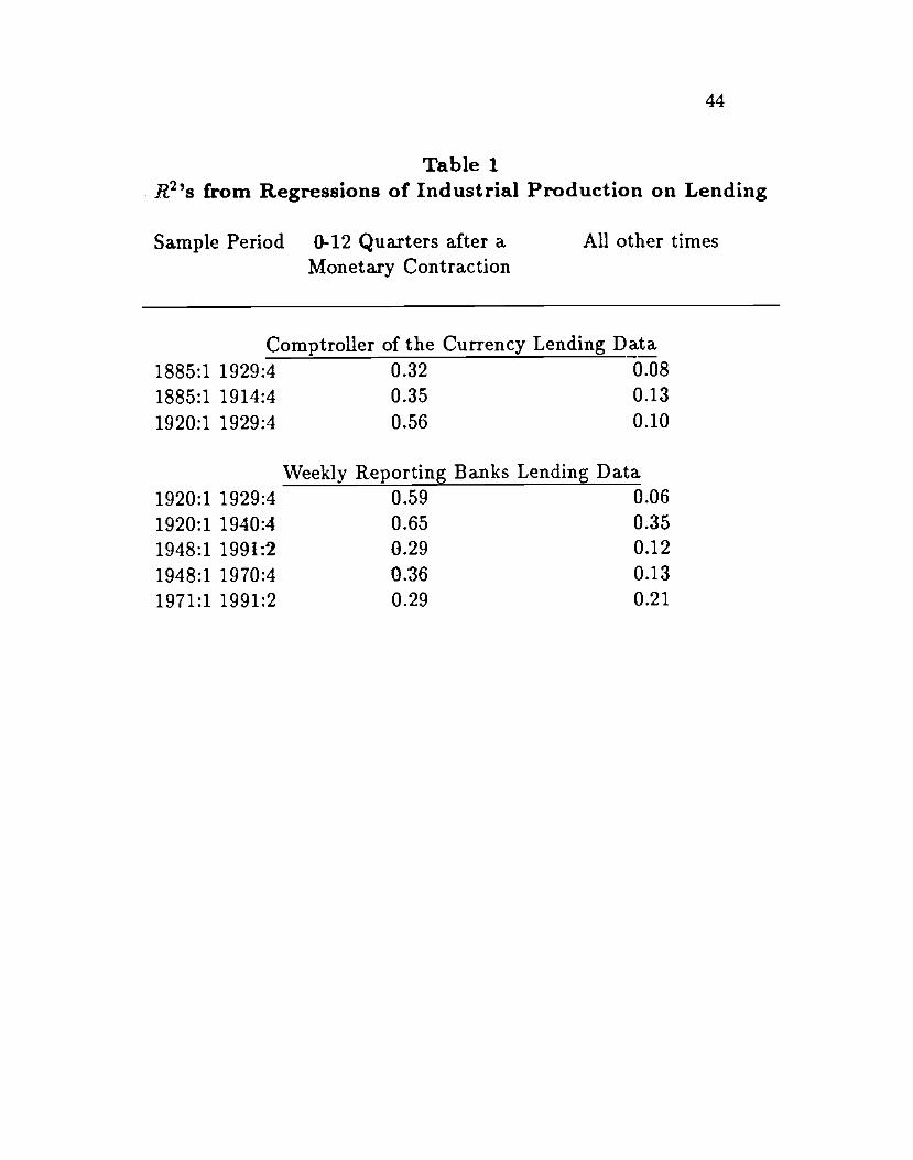
44

Table 1R2's from Regressions of Industrial Production on Lending

Sample Period 0-12 Quarters after a All other timesMonetary Contraction

Comptroller of the Currency Lending Data1885:1 1929:4 0.32 0.081885:1 1914:4 0.35 0.131920:1 1929:4 0.56 0.10

Weekly Reporting Banks Lending Data1920:1 1929:4 0.59 0.061920:1 1940:4 0.65 0.351948:1 1991:2 .0.29 0.121948:1 1970:4 0.36 0.131971:1 1991:2 0.29 0.21

45

:::

0.6

0.5

0.4

0.3

0.2

0.11896

Fig. 1 Ratio of Bank Loans to Total Interest-Bearing BatikAssets, 1896-1988

Note: Real estate loans are excluded from bank loans.

1907 1918 1929 1940 1951 1962 1973 1984

46

a. Ratio of Time Deposit to Demand Deposit Requirement

1.2

0.8

0.6-

189

b. Reserve Requirement on Time Deposits

0.3

0.25

0.2

0.15

874 1894 1914 1934 1954 1974

Fig. 2 Reserve Requirements, 1874-1991

a. Ratio of Time Deposits to Total Interest—Bearing Assets

0.8

0.7

0.6

0.5

0.4

0.3

0.2

0.1

b. Ratio of Bank Loans

2

1.8

1.6

1.4

1.2-

0.8

0.6

0.4

0.21896

Fig. 3 Composition of Bank Portfolios, 1896-1988

47

to Net Interest—Bearing Assets (Lambda)

1907 1913 140 1951 1962 1973 1984

0.3-

0.28-

0.26

0.24-

0.22

0.20.l80.16

0.14

0.1

Fig. 4 Ratio of Bank Loans to the Capital Stock, 1925-198S

48

925 1936 1947 1958 1969 1980

49

0.16

0.15

0.14

0.13

0.12

0.1 1

0.1

0.09

0.08

0.07

0.06

0.051900

Fig. 5 Ratio of Loans to Total Uabilities for Corporations, 1900-1989

Note: Before 1945 data are only available for starred observations;after 1945 the data are annual.

0.6

0.55

0.5

0.45

0.4

0.35

0.3

0.25

0.21900

Fig. 6 Ratio of Loans to Total Liabilities for UnincorporatedBusinesses, 1900-1945

Note: Data are only available for starred observations.

50

1911 1922 1933 1944

51

0.3

0.25

0.2

0.15

0.l

0.051900

Fig. 7 Ratio of Total Liabilities of Unincorporated Businesses toTotal Liabilities of Corporations, 1900-1989

Note: Before 1945 data are only available for starred observations;after 1945 the data are annual.

a. 1890—19096

5

4

3

2

0

—I

—2

—3

—4

b. 1910—1929

4

3

2

0

—2

—3

—41910

C. 1930—19386

5

4

3

2

0

—1

—2

—3

—4

Fig. 8 Loan-Bond Interest Rate Spread and MonetaryContractions, 1890-1991

52

6

5

1913 1916 1919 1922 1925 1928

1930 1933 1936

d. 1947—1970

—1

—2

—3 -

—4.——1947 1950

e. 1971—19916

5

3

2

0

—l

—2

—3

—4

Fig. 8 (Continued)

53

Note: Vertical lines denote the dates of negative monetary shocks.

6'5'4.

3-

2

I.0'

1953 19561959 1962 1965 1968

a. 1890—19294

3

2

0

—l

—2

—3

—4

b. 1930—19384

3

2

0

—l

—2

—3

—4

4

3

2

0

—2

C. 1947—1970

3

—4

54

Fig. 9 Average Response of the Spread to Monetary Contractions

—4 —2 0 2 4 6 8

—4 —2 0 2 4 6 8

—4 —2 0 4 8

d. 1971—1991

55

Fig. 9 (Continued)

Notes: The vertical line denotes the date of a negative monetaryshock. The average behavior of the spread is calculated for fourquarters before to eight quarters after the monetary shock.

4

3.

I.

0

—I

—2

—3.

—4.—4 —2 0 2 4 6 8

b. 1947—1970

0.95

0.9

0.85'

0.8'

0.75'

0.7917

C.

0.95

0.9

0.85

0.8

0.75

0.7197 I l97 1977 980 1983 1986 1989

Fig. 10 The Mix and Monetary Contractions, 1919-1991

a. 1919—1940

56

0.95'

0.9'

0.85'

0.8'

0.75-

0.7-—.—1919 1922 1925 1928 1931 1934 1937 1940

.

1950 1953 1956 1959 1962 1965 1968

1971—1991

_____

57

Fig 10 (Continued)

Notes: The mix is calculated as the ratio of bank loans outstandingto the sum of bank loans and commercial paper outstanding.Vertical lines denote the dates of negative monetary shocks.

58

DATA APPENDIX: Balance Sheet Data for Firms and Households

The basic sources for these data come from three sources: Gold-smith, Lipsey, and Mendelson (1963), the Board of Governors ofthe Federal Reserve System (1973), and the Board of Governors ofthe Federal Reserve System (1990). These sources are referred toas GLM, FRB 1973, and FRB 1990, respectively, in the followingdescriptions. We line up the data from GLM for Nonfinancial Cor-porations with the FRB series for Corporate, Nonfinancial Businessand the data from GLM on Nonfarm Unincorporated Businesses withthe FRB series on Nonfarm, Noncorporate Business.

The general strategy is to line up particular components of thebalance sheet that are of interest, such as total liabilities, bank loansnot elsewhere classified, and bonds and notes, from the diiTerentsources and then ratio splice them together. The ratio splices arenecessary because the series do not line up exactly due to slightchanges in concepts and measurement techniques over time. Thedata for 1966-1989 are from FRB 1990 and are taken as they are.The data for 1946-1966 are from FRB 1973 and are ratio spliced tothe modern data in 1966. The data for 1900-1945 are from GLM andare spliced on in 1945.

Nonfinancial Corporations. The balance sheet data for 1900-1945are given in GLM, Table III-4b, p. 146. The data for 1945-1966 arefrom FRB 1973, pp. 85-87. The data for 1966-1989 are from FRB1990, pp. 9-10. The GLM data include commercial paper liabilitiesin the bonds and notes category, while the FRB reports bonds andopen market paper separately (GLM, p. 10). We combine the twoto be the extension of the GLM series. Trade debt is gross for bothsources. The data for corporate equities for 1900-1945 is from GLM,Table IV-b-17b, pp. 318-319. The equities data for 1945-1966 arefrom FRB 1973, pp. 117-119 and for 1966-1989 are from FRB 1990,pp. 9-10.

Nonfarm, Unincorporated Businesses. We had hoped to form acontinuous balance sheet for nonfarm, unincorporated businesses aswell as for corporations. However, in 1945, the one year of overlap

59

between the two series, bank loans n.e.c. are roughly 9 timeslarger inthe GLM data than in the FRB data. Much of this difference appearsto be due to how total liabilities are allocated among categories.For this reason, we do not examine the individual elements of theunincorporated business sector. We do, however, use the data ontotal liabilities. The data for 1900-1945 are from GLM, Table III-2a,p.128. Data for 1945-1966 are from FRB 1973, pp. 85-87 and for1966-1989 from FRB 1990, pp. 7-8. Adjustment of the FRB series isneeded because for 1945-1966 the total liabilities series includes nettrade debt, while GLM and the later FRB series included gross tradedebt (GLM, p. 9). For these years we subtract net trade debt fromtotal liabilities and add in gross trade debt.