Experiment # 1

To determine the Manning’s Roughness Coefficient(n) & Chézy Coefficient(c) in laboratory flume

Purpose:

To study changes in Manning’s Roughness coefficient (n) by varying discharge (Q) in

flume.

To study changes in Chezy Coefficient(c) by varying discharge (Q) in flume.

To investigate relation between Manning Roughness Coefficient(n) & Chezy Coefficient

(c)

To determine Manning Roughness Coefficient(n) and Chezy Coefficient (c)

Apparatus :

i. S6 glass sided tilting flume

Note: In this type of flume we can adjust

positive as well as negative slope. Positive

slope ranges between 0 to 1:40 and negative

upto 1:200.The bad of the flume is made up of

cold formed steel. Length of the channel is 7.5

m.

ii. Point Gauge

iii. Differential Manometer

Related Theory:

1) Uniform Flow:

That type of flow in which flow perimeters and channel perimeters remain constant as

a function of distance between two cross sections. In uniform flow, depth and velocity

remain constant along the flow direction for the given discharge in the given channel. We

can say that it is only possible in prismatic channels.

2) Non-Uniform Flow:

That type of flow in which flow perimeters and channel perimeters do not remain

constant as a function of distance between two cross sections.

3) Steady flow:

That type of flow in which flow perimeters and channel perimeters remains constant at a

particular cross-section with respect to time.

4) Unsteady flow:

That type of flow in which flow perimeters and channel perimeters remains do not remain

constant at a particular cross-section with respect to time.It can also be determined by noting

the depth of water.

There are four different flow combinations present.

i. Uniform-Steady

Generally flow in irrigation canals are maintained uniform and steady.

ii. Non-uniform-Steady

A typical example of such flow is back water flow on upstream of the dam.

iii. Unsteady-Uniform

An example is a pipe of constant diameter connected to a pump pumping at a

constant rate which is then switched off. This type of flow is practically not possible

in open channel.

iv. Unsteady-Non-uniform

Example of this type of flow is flood waves.

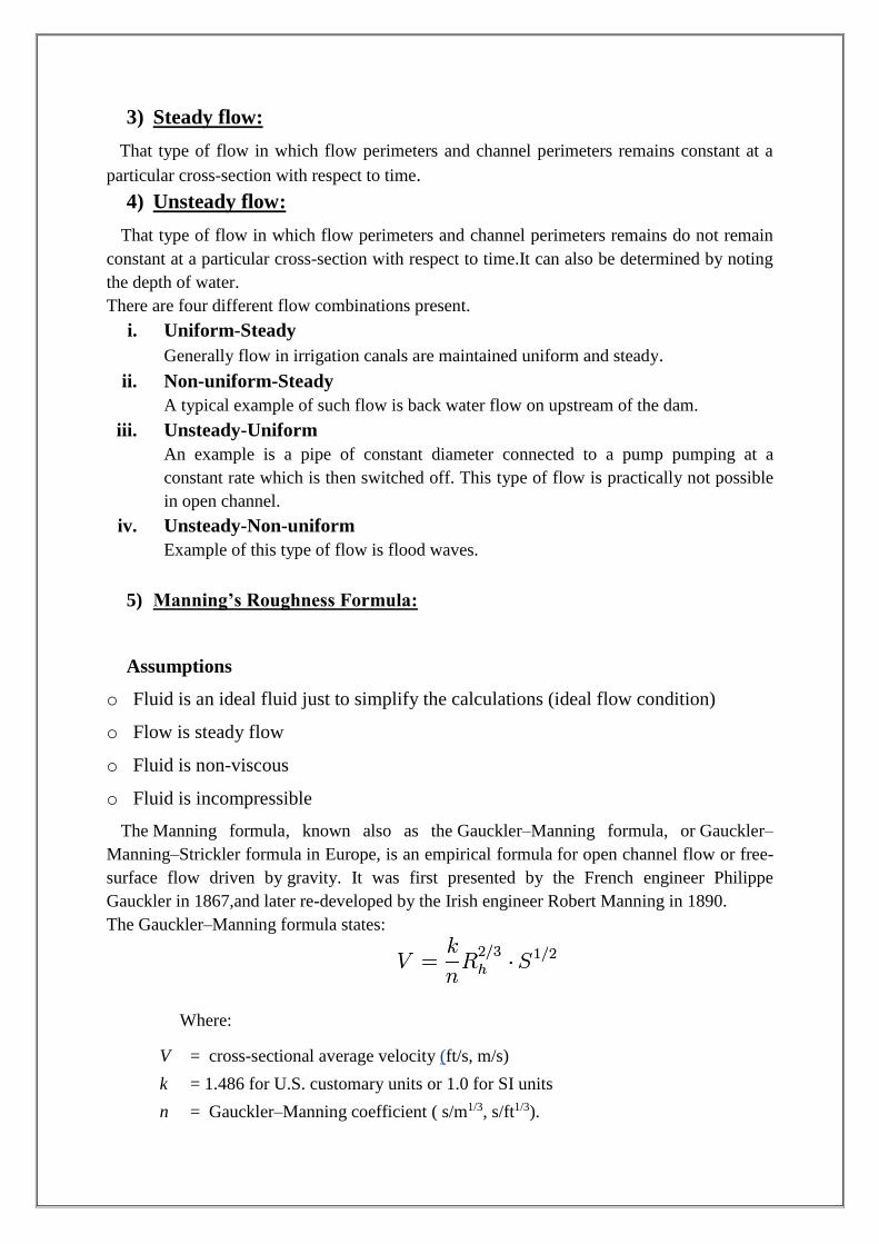
5) Manning’s Roughness Formula:

Assumptions

o Fluid is an ideal fluid just to simplify the calculations (ideal flow condition)

o Flow is steady flow

o Fluid is non-viscous

o Fluid is incompressible

The Manning formula, known also as the Gauckler–Manning formula, or Gauckler–

Manning–Strickler formula in Europe, is an empirical formula for open channel flow or free-

surface flow driven by gravity. It was first presented by the French engineer Philippe

Gauckler in 1867,and later re-developed by the Irish engineer Robert Manning in 1890.

The Gauckler–Manning formula states:

Where:

V = cross-sectional average velocity (ft/s, m/s)

k = 1.486 for U.S. customary units or 1.0 for SI units

n = Gauckler–Manning coefficient ( s/m1/3, s/ft1/3).

Rh = hydraulic radius (ft, m)

S = slope of the water surface or the linear hydraulic head loss (m/m.ft/ft)) (S = hf/L)

The Gauckler–Manning coefficient (n) depends upon roughness of the

channel,Vegitation,scavering and many other factors.

Hydraulic Radius (Rh) =A/P

P= wetted perimeter

A=area of flow of water

The discharge formula, Q = A V, can be used to manipulate Gauckler–Manning's equation

by substitution for V. Solving for Q then allows an estimate of the volumetric flow

rate (discharge) without knowing the limiting or actual flow velocity.

The Gauckler–Manning formula is used to estimate flow in open channel situations where it

is not practical to construct a weir or flume to measure flow with greater accuracy. The

friction coefficients across weirs and orifices are less subjective than “n” along a natural

(earthen, stone or vegetated) channel reach. Cross sectional area, as well as “n”, will likely

vary along a natural channel.

6) Effect of Gauckler–Manning coefficient(n) on channel:

The effect of Gauckler–Manning coefficient (n) on flow is very important because if value

of Gauckler–Manning coefficient (n) changes from the original value it will cause many

problems and efficiency of channel will decrease.

If Gauckler–Manning coefficient (n) increases velocity of water will decrease and due to

which sedimentation will increase,it will raise the bed channel and there are chances of over

flow of water. On the other hand if Gauckler–Manning coefficient (n) decreases than it will

increase the velocity and head depth of water will decreases. It will effect whole system of

irrigation as well as the hydro power projects.

7) Chezy Formula:

The Chézy formula describes the mean flow velocity of steady, turbulent open

channel flow:

v = c √(R S)

Where

v = mean velocity (m/s, ft/s)

c = the Chezy roughness and conduit coefficient

R = hydraulic radius of the conduit (m, ft)

S = slope of the conduit (m/m, ft/ft)

The formula is named after Antoine de Chézy, the French hydraulics engineer who

devised it in 177.

8) Relation between Mannning’s roughness coefficient and Chezy

Coefficient:

This formula can also be used with Manning's Roughness Coefficient, instead of

Chézy's coefficient. Manning derived the following relation to C based upon

experiments:

Where

“C” = the Chézy coefficient [m½/s],

“R” = the hydraulic radius [m],

“n” = Manning's roughness coefficient.

This relation is empirical.

Procedure:

i. Set the slope of the channel.

ii. Switched on the pump and left it to become fully operational.

iii. After some time uniform condition is achieved.

iv. Note down the manometric head attached to the flume and find the discharge

from the table provided by the Manufacturer.

v. Also we will note done the average depth of water in the flume by gauge by

measuring depth at 2,4,6 m .

vi. Repeat the same procedure for different values of discharge.

Observations and Calculations

Formulas

Manning’s formula

vavg=𝛼

𝑛1× Rh

2/3× S0

1/2

vavg=𝛼

𝑛2× Rh

2/3× S1/2

Chaezy’s formula

vavg =𝑐1√𝑅𝑆0

vavg =𝑐2√𝑅𝑆

Hydraulic radius =Rh = A/P ; Area of flow of water= A=b x yavg

Depth = yavg = (y1+y2+y3)/3 ; Wetted perimeter = P = b + 2yavg

S = Slope of Energy line ; Sw= Slope of Hydraulic Grade Line

S0=Slope of Channal Bed ; vavg= Average Velocity

For uniform flow conditions S = S0 = Sw

α =Conversion Constant = 1.00 in SI = 1.486 in FPS

n = Manning’s Roughness Coefficient; c = Chezy Coefficient

Sr No

So Q y A vavg S Pw Rh

Manning’s Roughness coefficient

Chezy’s Coefficient

y1 y2 y3 yavg n1 n2 c1 c2

(m3/s) (m) (m) (m) (m) (m2) (m/s) (m) (m) (s/m1/3) (s/m1/3) (m1/2/s) (m1/2/s)

1 0.002 0.008942 0.055 0.059 0.06 0.058 0.0174 0.513908 0.001 0.416 0.041827 0.010486 0.010486 56.18786 79.46163

2 0.002 0.011997 0.072 0.073 0.073 0.072667 0.0218 0.550321 0.00055 0.445333 0.048952 0.010875 0.010875 55.61802 106.0594

3 0.002 0.015996 0.079 0.081 0.079 0.079667 0.0239 0.669289 0.00045 0.459333 0.052032 0.009313 0.009313 65.60902 138.316

4 0.002 0.018326 0.084 0.083 0.081 0.082667 0.0248 0.738952 0.0003 0.465333 0.053295 0.008571 0.008571 71.57432 184.8041

5 0.002 0.0192 0.084 0.087 0.085 0.0853 0.0256 0.7610 0.0005 0.7521 0.749141 0.0005 0.470667 0.054391 0.00857

6 0.002 0.0204 0.092 0.092 0.085 0.0897 0.0269 0.7388 0.0011 0.7996 0.75803 0.0011 0.479333 0.05612 0.008648

0

20

40

60

80

100

120

140

160

180

200

0.0000 0.0050 0.0100 0.0150 0.0200 0.0250

c2

(m1

/2/s

)

Q(m3/s)

Relation bettwen Q & c2

0.0000

0.0050

0.0100

0.0150

0.0200

0.0250

0 0.002 0.004 0.006 0.008

Q(m

3/s

)

n2

(s/m)

Relation between Q & n2

0

0.001

0.002

0.003

0.004

0.005

0.006

0.007

0.008

0 50 100 150 200

n2

(s/m

1/3

)

c2

(m1/2/s)

Relation between n2 & c2

2, 0.0700 4, 0.0720 6, 0.0726

2, 0.0554, 0.059 6, 0.06

0.0000

0.0100

0.0200

0.0300

0.0400

0.0500

0.0600

0.0700

0.0800

0 1 2 3 4 5 6 7

He

ad(m

)

Horizontal Distance(m)

Hyraulic Grade Line & Energy Line # 1

EL 1

HGL 1

2, 0.1022 4, 0.1031 6, 0.1022

2, 0.079 4, 0.081 6, 0.079

0.0000

0.0200

0.0400

0.0600

0.0800

0.1000

0.1200

0 1 2 3 4 5 6 7

He

ad(m

)

Horizontal Distance(m)

Hyraulic Grade Line & Energy Line # 3

EL

HGL

2, 0.0877 4, 0.0883 6, 0.0883

2, 0.072 4, 0.073 6, 0.073

0.0000

0.0100

0.0200

0.0300

0.0400

0.0500

0.0600

0.0700

0.0800

0.0900

0.1000

0 1 2 3 4 5 6 7

He

ad(m

)

Horizontal Distance(m)

Hyraulic Grade Line & Energy Line # 2

EL

HGL

2, 0.1198 4, 0.1198 6, 0.1176

2, 0.084 4, 0.087 6, 0.085

0.0000

0.0200

0.0400

0.0600

0.0800

0.1000

0.1200

0.1400

0 1 2 3 4 5 6 7

He

ad(m

)

Horizontal Distance(m)

Hyraulic Grade Line & Energy Line # 5

EL

HGL

2, 0.1110 4, 0.1106 6, 0.1100

2, 0.084 4, 0.083 6, 0.081

0.0000

0.0200

0.0400

0.0600

0.0800

0.1000

0.1200

0 1 2 3 4 5 6 7

He

ad(m

)

Axis Title

Hyraulic Grade Line & Energy Line # 4

EL

HGL

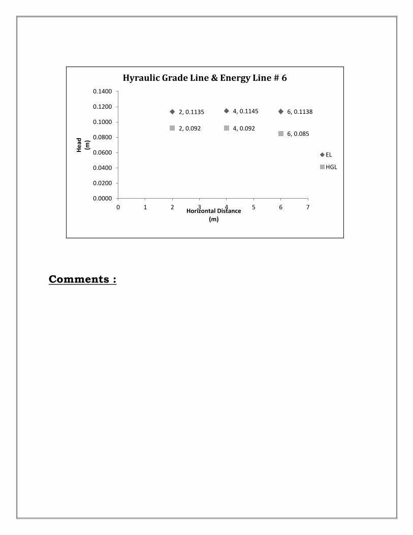
2, 0.1135 4, 0.1145 6, 0.1138

2, 0.092 4, 0.0926, 0.085

0.0000

0.0200

0.0400

0.0600

0.0800

0.1000

0.1200

0.1400

0 1 2 3 4 5 6 7

He

ad(m

)

Horizontal Distance(m)

Hyraulic Grade Line & Energy Line # 6

EL

HGL

Comments :