mantle pseudo-isochrons revisited - core · mantle pseudo-isochrons revisited john f. rudge ⁎...

tters 249 (2006) 494–513www.elsevier.com/locate/epsl

Earth and Planetary Science Le

Mantle pseudo-isochrons revisited

John F. Rudge ⁎

Bullard Laboratories, Department of Earth Sciences, University of Cambridge, Madingley Road, Cambridge, CB3 0EZ, UKDepartment of Applied Mathematics and Theoretical Physics, Centre for Mathematical Sciences, Wilberforce Road, Cambridge CB3 0WA, UK

Received 15 December 2005; received in revised form 26 June 2006; accepted 27 June 2006Available online 23 August 2006

Editor: R.D. van der Hilst

Abstract

The 2.0 Ga pseudo-isochron age inferred from the mid-ocean ridge basalt 207Pb/204Pb against 206Pb/204Pb diagram is re-examined on the basis of a statistical box model of mantle processes. Simple equations are presented which relate the pseudo-isochron age to the decay constants and distribution of heterogeneity ages in the model mantle. In turn this age distribution issimply related to the history of melting. The equations are in good agreement with results from mantle convection simulations. Theequations are different from but related to, and more general than, those found previously for mean box models. While the pseudo-isochron age does not signify a mean age in the usual sense, in the model presented it is related to a “generalised mean” over thedistribution of heterogeneity ages. If a constant melt rate over the Earth's history is assumed, a mean remelting time of 0.5 Ga isrequired.© 2006 Elsevier B.V. All rights reserved.

Keywords: mantle; isochron; isotope ratios; heterogeneity; stirring; mixing

1. Introduction

When 207Pb /204Pb is plotted against 206Pb /204Pb fordata frommid-ocean ridge basalt (MORB) or ocean islandbasalt (OIB) an approximate linear relationship is found(Fig. 1). The slope of a regression line through these datapoints can be used to infer an age by treating the re-gression line as if it were an isochron [1,2]. Formally anisochron age dates a single fractionation event, which isnot the case for MORB and OIB; the isotopic systematicsof these basalts result from multiple fractionations due torepeated melting and recycling over the course of theEarth's history. As such the ages calculated by the iso-

⁎ Fax: +44 1223 360779.E-mail address: [email protected].

0012-821X/$ - see front matter © 2006 Elsevier B.V. All rights reserved.doi:10.1016/j.epsl.2006.06.046

chron method are often referred to as pseudo-isochronages, and the aim of this work is to relate the pseudo-isochron ages to real physical parameters.

The isotopic systems we will study consist of a parentisotope p which decays to a daughter isotope d withdecay constant λ. There is a reference isotope d′ withrespect to which these isotopes are measured. Thereference isotope is of the same element as the daughterd, but neither decays nor is a decay product. There aretwo particular isochrons we will focus on, and we willrefer to these as the parent–daughter isochron and thedaughter–daughter isochron.

The parent–daughter isochron involves plotting d/d′against p/d′. The parent–daughter isochron age τpdi isrelated to the slope β of the regression line by

ekspdi−1 ¼ b: ð1Þ

mailto:[email protected]

http://dx.doi.org/10.1016/j.epsl.2006.06.046

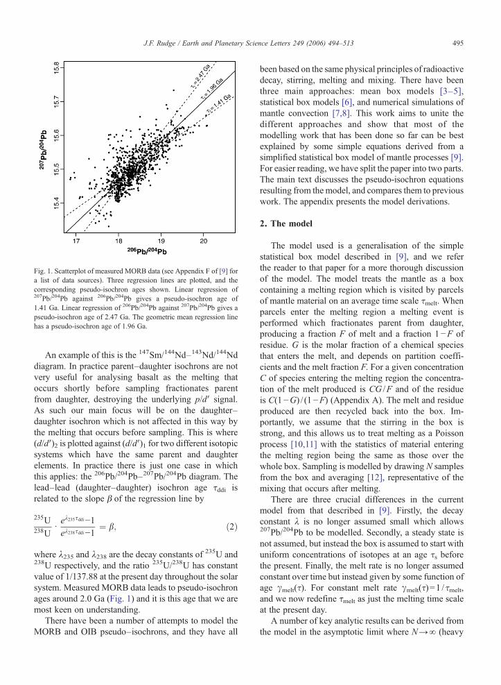
Fig. 1. Scatterplot of measured MORB data (see Appendix F of [9] fora list of data sources). Three regression lines are plotted, and thecorresponding pseudo-isochron ages shown. Linear regression of207Pb/204Pb against 206Pb/204Pb gives a pseudo-isochron age of1.41 Ga. Linear regression of 206Pb/204Pb against 207Pb/204Pb gives apseudo-isochron age of 2.47 Ga. The geometric mean regression linehas a pseudo-isochron age of 1.96 Ga.

495J.F. Rudge / Earth and Planetary Science Letters 249 (2006) 494–513

An example of this is the 147Sm/144Nd–143Nd/144Nddiagram. In practice parent–daughter isochrons are notvery useful for analysing basalt as the melting thatoccurs shortly before sampling fractionates parentfrom daughter, destroying the underlying p/d′ signal.As such our main focus will be on the daughter–daughter isochron which is not affected in this way bythe melting that occurs before sampling. This is where(d/d′)2 is plotted against (d/d′)1 for two different isotopicsystems which have the same parent and daughterelements. In practice there is just one case in whichthis applies: the 206Pb/204Pb–207Pb/204Pb diagram. Thelead–lead (daughter–daughter) isochron age τddi isrelated to the slope β of the regression line by

235U238U

dek235sddi−1ek238sddi−1

¼ b; ð2Þ

where λ235 and λ238 are the decay constants of235U and

238U respectively, and the ratio 235U/238U has constantvalue of 1/137.88 at the present day throughout the solarsystem. Measured MORB data leads to pseudo-isochronages around 2.0 Ga (Fig. 1) and it is this age that we aremost keen on understanding.

There have been a number of attempts to model theMORB and OIB pseudo–isochrons, and they have all

been based on the same physical principles of radioactivedecay, stirring, melting and mixing. There have beenthree main approaches: mean box models [3–5],statistical box models [6], and numerical simulations ofmantle convection [7,8]. This work aims to unite thedifferent approaches and show that most of themodelling work that has been done so far can be bestexplained by some simple equations derived from asimplified statistical box model of mantle processes [9].For easier reading, we have split the paper into two parts.The main text discusses the pseudo-isochron equationsresulting from the model, and compares them to previouswork. The appendix presents the model derivations.

2. The model

The model used is a generalisation of the simplestatistical box model described in [9], and we referthe reader to that paper for a more thorough discussionof the model. The model treats the mantle as a boxcontaining a melting region which is visited by parcelsof mantle material on an average time scale τmelt. Whenparcels enter the melting region a melting event isperformed which fractionates parent from daughter,producing a fraction F of melt and a fraction 1−F ofresidue. G is the molar fraction of a chemical speciesthat enters the melt, and depends on partition coeffi-cients and the melt fraction F. For a given concentrationC of species entering the melting region the concentra-tion of the melt produced is CG /F and of the residueis C(1−G) / (1−F) (Appendix A). The melt and residueproduced are then recycled back into the box. Im-portantly, we assume that the stirring in the box isstrong, and this allows us to treat melting as a Poissonprocess [10,11] with the statistics of material enteringthe melting region being the same as those over thewhole box. Sampling is modelled by drawing N samplesfrom the box and averaging [12], representative of themixing that occurs after melting.

There are three crucial differences in the currentmodel from that described in [9]. Firstly, the decayconstant λ is no longer assumed small which allows207Pb/204Pb to be modelled. Secondly, a steady state isnot assumed, but instead the box is assumed to start withuniform concentrations of isotopes at an age τs beforethe present. Finally, the melt rate is no longer assumedconstant over time but instead given by some function ofage γmelt(τ). For constant melt rate γmelt(τ)=1 /τmelt,and we now redefine τmelt as just the melting time scaleat the present day.

A number of key analytic results can be derived fromthe model in the asymptotic limit where N→∞ (heavy

496 J.F. Rudge / Earth and Planetary Science Letters 249 (2006) 494–513

averaging), and all the results in the next section arebased on this limit (Appendices B and C). Numericalsimulation suggests that the dependence of the pseudo-isochron age on N is fairly weak (Fig. 2), and so usingthe N→∞ asymptotics seems well justified. In this limitthe distribution of isotopic ratios tends to a multivari-ate normal distribution, and expressions for the corre-sponding covariance matrix can be derived. In particularthese expressions allow us to estimate the slopes ofregression lines in plots of one isotopic ratio againstanother, and thus to derive expressions for the modelpseudo-isochron ages.

There are many different ways of fitting a line to acloud of data points. Following [3] we have focused onthe geometric mean regression line (also known as thereduced major axis regression line) whose slope is givenby the ratio of the standard deviations of the two isotopicratios in question (solid line in Fig. 1). To give anestimate of the uncertainty in fitting a line we have alsoincluded results from using the two linear regressionlines (dotted lines in Fig. 1) in some of the figures. If thecorrelation is good all three lines should be similar.

3. The pseudo-isochron equations

The key to determining the pseudo-isochron ages inthe model is the random variable Tm which gives thedistribution of parcel ages for those parcels that havepassed through the melting region. The age of a parcel isdefined as the time since last visit to the melting region.The parcels that have not visited the melting region are

Fig. 2. Constant melt rate model numerical simulations with N=1, 500, and 2Partition coefficients are those used in [9], giving GPb=0.42 and GU=1.00measured MORB data (Fig. 1). The left picture shows unaveraged compositioellipse under heavy averaging, indicative of a bivariate normal distributionregression line for the three cases leads to pseudo-isochron ages of 2.30 Ga, 1an age of 2.03 Ga as N→∞.

referred to as primordial parcels, and are not assigned anage. Let E be an expectation over a random variable, sothat

Ef ðTmÞ ¼Z ss

0f ðsÞqmðsÞds; ð3Þ

where qm(τ) is the probability density function of par-cel ages, and f (τ) is an arbitrary given function. Thesubscript ‘m’ is to emphasise that we consider only thoseparcels that have passed through the melting region. Inthis model the primordial parcels make no contributionto the pseudo-isochron ages, since primordial parcelshave uniform isotopic concentrations equal to the meanover the whole box. In terms of Tm the model pseudo-isochron equations are simply (Appendices D and E)

ðekspdi−1Þ2 ¼ Eðek Tm−1Þ2; ð4Þ

ðek235sddi−1Þ2ðek238sddi−1Þ2 ¼

Eðek235 Tm−1Þ2Eðek238 Tm−1Þ2

; ð5Þ

where τpdi and τddi are the parent–daughter and lead–leadpseudo-isochron ages respectively. Note that theseexpressions depend only on the decay constants andthe distribution of parcel ages. The expressions clearlyshow that the pseudo-isochron ages are just particularweighted averages over the parcel ages. In fact thepseudo-isochron ages are examples of “generalisedmeans” [13,14] (Appendix F). It also follows from theseexpressions that the pseudo-isochron ages are always

5,000, τmelt=0.75 Ga, τs=3.0 Ga, F=1.5%, and a sample size of 1000.((2) of [9]). The middle picture has similar variance and slope as thens, the right heavily averaged compositions. Note that the data forms anas expected by the central limit theorem [17]. The geometric mean.98 Ga, and 2.06 Ga respectively. The pseudo-isochron Eq. (8) predicts


greater than or equal to sm ¼ ETm the mean age of parcelsthat have passed through the melting region. This is animportant result as it means that models with τm greaterthan the observed lead–lead pseudo-isochron age ofaround 2.0 Ga cannot be compatible with the isotopicobservations (such as the Daviesmodel [15]). If the parcelages≪1/λ then Eq. (4) reduces to spdi ¼

ffiffiffiffiffiffiffiffiET

2m

q, a result

which is independent of λ. Hence, parent–daughterpseudo-isochron ages will be the same for all slowlydecaying isotopes, namely for the 147Sm/144Nd–143Nd/144Nd, 87Rb/86Sr–87Sr/86Sr, 176Lu/177Hf–176Hf/177Hf,and 232Th/204Pb–208Pb/204Pb diagrams.

The history of the rate of melting can be directlyrelated to the distribution of parcel ages in the model. Ifγmelt(τ) is the melt rate as a function of age then qmðsÞ ¼qðsÞ= R ss

0 qðsÞds where (Appendix G)

qðsÞ ¼ gmeltðsÞexp −Z s

0gmeltðsÞds

� �: ð6Þ

An important special case is wheremelt rate is constantγmelt(τ)=1/τmelt, where τmelt is a constant melting time

Fig. 3. Plot showing the variation of 147Sm/144Nd–143Nd/144Nd (λ=0.00654 Gbe produced for other isotopic systems where the decay is linearisable (τmelt o232Th/204Pb–208Pb/204Pb. (a) plots τpdi against start age τs for different valuesslope ¼ 1=

ffiffiffi3

p. The curves shown asymptote to

ffiffiffi2

psmelt for large values of τs

for different values of τs. Values of τs=2.5 Ga, 3.6 Ga and 4.5 Ga have been c[7,8]. For small values of τmelt the curves have a slope of

ffiffiffi2

p. For large val

2.08 Ga and 2.60 Ga respectively (fss=ffiffiffi3

p). Shown in grey is the uncertai

(solid line) lies between the two linear regression ages which bound the greybeen plotted as they substantially overlap the 3.6 Ga region.

scale. In this case qmðsÞ ¼ e−s=smelt=ðsmeltð1−e−ss=smeltÞÞand the model parent–daughter pseudo-isochron equationis (Appendix H)

ðekspdi−1Þ2 ¼R ss0 ðeks−1Þ2e−s=smeltds

smeltð1−e−ss=smeltÞ : ð7Þ

The most important feature of this equation is thatit depends only on the three time scale parameters inthe problem: the melting time scale τmelt, the start age τs,and the decay constant λ; and not on any of theother parameters. Fig. 3 plots solutions to Eq. (7) for143Nd/144Nd–147Sm/144Nd (λ=0.00654 Ga−1) in twodifferent ways. Fig. 4 shows similar graphs for 235U/204Pb–207Pb/204Pb (λ=0.985 Ga−1), a case for whichthe decay is not linearisable. Note that there is areasonable uncertainty in the parent–daughter pseudo-isochron ages indicated by the wide grey region in Figs.3b and 4b. This expected (and indeed observed) lack ofvery good correlation is another reason why parent–daughter pseudo-isochron ages are not particularlyuseful.

a−1) model pseudo-isochron age τpdi Eq. (7). Near identical curves willr τs≪1/λ), such as 87Rb/86Sr–87Sr/86Sr, 176Lu/177Hf–176Hf/177Hf, andof the melting time scale τmelt. For small values of τs the curves havewith the exception of the τmelt=∞ Ga curve. (b) plots τpdi against τmelt

hosen for comparison with numerical simulations of mantle convectionues of τmelt the curves asymptote to pseudo-isochron ages of 1.45 Ga,nty in fitting a line for τs=3.6 Ga: the geometric mean regression ageregion. The corresponding regions for τs=2.5 Ga and 4.5 Ga have not

Fig. 4. As Fig. 3 but for 235U/204Pb–207Pb/204Pb (λ=0.985 Ga−1), where the decay is not lineariseable. (a) plots τpdi against τs for different values ofτmelt. For τmeltb1/2λ=0.51 Ga the curves flatten out for large τs. For τmeltN1/2λ the curves grow linearly with τs for large τs. The τmelt=∞ Ga curveapproaches a slope of 1 for large τs. (b) plots τpdi against τmelt for different values of τs. For large values of τmelt the curves asymptote to pseudo-isochron ages of 1.73 Ga, 2.63 Ga and 3.40 Ga respectively.

Fig. 5. As Fig. 3 but for the 206Pb/204Pb–207Pb/204Pb (λ238=0.155 Ga−1, λ235=0.985 Ga−1) model pseudo-isochron age τddi Eq. (8). (a) plots τddiagainst τs for different values of τmelt. For small values of τs the curves have slope=0.75. For values of τmelt around 1–2 Ga the approximaterelationship τddi≈0.75τs holds for the range of τs plotted. For τmeltb1/2λ235=0.51 Ga the curves flatten out for large τs. For τmeltN1/2λ235 the curvesgrow linearly with τs for large τs. The τmelt =∞ Ga curve approaches a slope of 1 for large τs. (b) plots τddi against τmelt for different values of τs. Forsmall values of τmelt the curves have a slope of 3. For large values of τmelt the curves asymptote to pseudo-isochron ages of 2.02 Ga, 2.99 Ga and3.81 Ga respectively. Shown in grey is the uncertainty in fitting a line for each of the τs values.



The more useful pseudo-isochron equation is thelead–lead pseudo-isochron equation given for constantmelt rate by (Appendix I)


R ss0 ðek235s−1Þ2e−s=smeltdsR ss0 ðek238s−1Þ2e−s=smeltds

: ð8Þ

Fig. 5 plots solutions to Eq. (8). Note that the lead–lead pseudo-isochron ages are fairly well constrained asthe model correlation is good (as indicated by thenarrow grey regions of Fig. 5b).

The pseudo-isochron equations only encode age in-formation, and do not involve the parameters G and F.However, if we are concerned with the variance ofisotopic ratios, or the slopes in plots of one isotopic ratioagainst another which do not have common parent anddaughter elements, then these parameters are involved.This was the main focus of [9], and the correspondinggeneralisation of (1) of [9] for the standard deviation σof d/d′ ratios after sampling is (Appendix C)

r ¼ p

d Vd

jGp−GdjffiffiffiffiffiffiffiffiffiffiffiffiffiffiffiffiffiffiffiNFð1−FÞp d

ffiffiffiffiffiffiffiffiffiffiffiffiffiffiffiffiffiffiffiffiffiffiffiffiffiffiffiffiffiffiffiffiffiffiffiffiffiffiffiZ ss

0ðeks−1Þ2qðsÞds;

sð9Þ

where p/d ′ is the ratio of mean parent isotope concen-tration to mean reference isotope concentration over thewhole box at the present day.

4. Linear pseudo-isochron equations

There are three models based on linear evolutionequations that have recently been proposed for thepseudo-isochrons [3–5]. In fact, all three modelsproduce identical pseudo-isochron equations and areclosely related. Albarède [4] and Donnelly et al. [5] bothconsider a two reservoir model, and derive the pseudo-isochron equations in precisely the same way. Allègreand Lewin [3] consider a different set of linear evolutionequations for isotopic dispersion, which with somerearranging are almost equivalent to the two interactingreservoir equations.

The governing equations for two interacting reser-voirs derived by [4] and [5] are

dn1dt

¼ −n1s1

þ n2s2

−kn1; ð10Þ

dn2dt

¼ n1s1

−n2s2

−kn2; ð11Þ

dm1

dt¼ −

m1

h1þ m2

h2þ kn1; ð12Þ

dm2

dt¼ m1

h1−m2

h2þ kn2; ð13Þ

ds1dt

¼ −s1h1

þ s2h2

; ð14Þ

ds2dt

¼ s1h1

−s2h2

; ð15Þ

where the notation of [4] has been followed. ni, mi andsi are the total number of moles of parent, daughter andreference isotopes respectively in reservoir i (theseshould not be confused with p, d and d′ used throughoutthe appendix to represent concentrations). τi is theresidence time of the parent element in reservoir i, θi thecorresponding residence time for the daughter element.Let

Pn,P

m andP

s be the total number of moles ofparent, daughter and reference isotopes in bothreservoirs:

Pn=n1+n2,

Pm=m1+m2, and

Ps= s1+ s2.

Then

dP

n

dt¼ −k

Xn;

dP

m

dt¼ k

Xn;

dP

s

dt¼ 0; ð16Þ

and the governing equations for reservoir 1 can berewritten as

dn1dt

¼ −n1sþP

n

s2−kn1; ð17Þ

dm1

dt¼ −

m1

hþP

m

h2þ kn1; ð18Þ

ds1dt

¼ −s1hþP

s

h2; ð19Þ

where τ and θ are the relaxation times of the twoelements: the harmonic means of the residence times inthe two reservoirs

1s¼ 1

s1þ 1s2

;1h¼ 1

h1þ 1h2

: ð20Þ

We now rewrite these equations for closer compar-ison with [3]. Introduce new variables n⋆1 andm

⋆1 defined

by

n⋆1 ¼1Ps

n1−s1ns

� �1þ2

� �; ð21Þ

m⋆1 ¼

1Ps

m1−s1ms

� �1þ2

� �; ð22Þ


where the subscript 1+2 refers to the total system:(n/s)1 + 2=

Pn=

Ps and (m/s)1 + 2=

Pm=

Ps. Note that

n⋆2 ¼ −n⋆1 and m⋆2 ¼ −m⋆

1. The governing equations inthe starred variables can then be written as

dn⋆1dt

¼ 1

s2−1

h2

� �n

s

� �1þ2

−kn⋆1−1Ps

n1s−s1h

n

s

� �1þ2

� �;

ð23Þdm⋆

1

dt¼ kn⋆1−

m⋆1

h: ð24Þ

These governing equations take on a particularlysimple form if the relaxation times for parent anddaughter elements are the same, τ=θ=1 /γ say. For laterconvenience, define gn=τ /τ1 and gm=θ /θ1, and notethat 0≤gn, gm≤1. Then

dn⋆1dt

¼ −ðgn−gmÞg ns

� �1þ2

−ðkþ gÞn⋆1; ð25Þ

dm⋆1

dt¼ kn⋆1− gm⋆

1: ð26Þ

These can be compared to the governing Eqs. (1) and(2) of Allègre and Lewin [3]

dhliðtÞdt

¼ AðtÞ−ðkþMðtÞÞhliðtÞ; ð27Þ

dhaiðtÞdt

¼ khliðtÞ þ BðtÞ−MðtÞhaiðtÞ: ð28Þ

These governing equations are identical to Eqs. (25)and (26) if the chemical dispersion hliðtÞ ¼ n⋆1, theisotopic dispersion haiðtÞ ¼ m⋆

1, the rate of injection ofchemical heterogeneity A(t)=− (gn−gm)γ(n/s)1 + 2, therate of injection of isotopic heterogeneity B(t)=0, andthe stirring parameter M(t)=γ. The appendix of [3]discusses solutions to these equations in the simplifiedform ((A1-1) and (A1-2) of [3])

dhliðtÞdt

¼ Dhlie−ktR

−ðkþ s−1stirÞhliðtÞ; ð29Þ

dhaiðtÞdt

¼ khliðtÞ þ DhaiR

−haiðtÞsstir

; ð30Þ

where by comparison Δ⟨μ⟩/R=− (gn−gm)γ(n/s)1 + 2(0),Δ⟨α⟩=0, and τstir =γ

− 1. These are solved subject toinitial conditions ⟨μ⟩(0)=0, ⟨α⟩(0)=0 which corre-sponds to the two reservoirs having initially identicalisotopic ratios (n/s)1(0)= (n/s)2(0)= (n/s)1 + 2(0) and (m/s)1(0)= (m/s)2(0)= (m/s)1 + 2(0). Allègre and Lewin de-

fine the slope of their parent–daughter pseudo-isochronby the ratio ⟨α⟩(t)/⟨μ⟩(t). However,

haiðtÞhliðtÞ ¼

m⋆1

n⋆1¼ m1−s1ðm=sÞ1þ2

n1−s1ðn=sÞ1þ2

¼ ðm=sÞ1−ðm=sÞ1þ2

ðn=sÞ1−ðn=sÞ1þ2

: ð31Þ

Hence the definition of the slope by the ratio ⟨α⟩(t)/⟨μ⟩(t) is the same as the slope of the line through thereservoirs 1, 2 and 1+2 on the parent–daughter isochrondiagram. Thus provided the relaxation times are equalin the two reservoir model, and there is no excessisotopic heterogeneity Δ⟨α⟩ in the Allègre and Lewinmodel, the pseudo-isochron equations are exactly thesame. Importantly, the stirring time τstir of Allègre andLewin can be reinterpreted as the common relaxationtime in the two reservoir model.

In one sense the Allègre and Lewin model is moregeneral than the two reservoir model because of theexcess isotopic heterogeneity term Δ⟨α⟩, but in practicethis was always set to zero for their pseudo-isochroncalculations. On the other hand, the two reservoir modelcan be thought of as more general since it allows theparent and daughter elements to have different relaxa-tion times. If parent and daughter are fractionated by thesame melting process we might expect relaxation timesto be the same. Also, note that in secular equilibriumonly the relaxation time θ of the daughter elementdetermines the pseudo-isochron [4].

Standard deviations are not conservative and shouldnot be modelled by linear evolution equations such asEqs. (27) and (28). The justification of these equationsby Allègre and Lewin is rather ad hoc. The two reservoirmodel and the Allègre and Lewin model are both linearmodels and thus essentially concerned with meanvalues, whereas standard deviations are fundamentallynonlinear. In the statistical box model it is possible todiscuss standard deviations, variances and covariances,as well as means, because the underlying probabilitydistributions are being modelled. Note that the starredvariables which relate the Allègre and Lewin model tothe two reservoir model arise naturally from thelinearisation

xy−xyc

1y

x−yxy

� �; ð32Þ

valid for |x− x|≪ x and |y− y|≪ y. The starred variablesturn out to be particularly useful when consideringasymptotics for large N in the statistical box model(Appendix B).


We can make an important connection betweenthe statistical box model and the two reservoir modelby dividing the parcels in the box into two groupings.Labelling the residue parcels and a fraction 1-F ofthe primordial parcels as one reservoir, and the meltparcels and a fraction F of the primordial parcels asanother reservoir, gives a two reservoir system with acommon relaxation time. The connection is made ifγ=γmelt, gn=Gp and gm=Gd (Appendix J). Further-more, this suggests an alternative way of writing thelinear pseudo-isochron equations of Allègre and Lewinin terms of an age distribution. These are the same asEqs. (4) and (5) except with the squareds removed

ekspdil−1 ¼ Eðek Tm−1Þ; ð33Þ

ek235sddil−1ek238sddil−1

¼ Eðek235 Tm−1ÞEðek238 Tm−1Þ

; ð34Þ

where τpdil and τddil are the linear parent–daughter andlead–lead pseudo-isochron ages respectively. It shouldbe noted that the linear pseudo-isochron ages willalways be less than the corresponding ages obtainedfrom Eqs. (4) and (5). The pseudo-isochron Eqs. (4) and(5) for our problem are different because they involvethe variance of a mixture of melt, residue and primordialparcels, whereas the above equations result from meanvalues of reservoirs. The squareds reflect the differencebetween looking at a mean value and looking at avariance. To emphasise the similarities and differencesbetween the linear pseudo-isochron equations and ourpseudo-isochron equations, Figs. 3–5 mimic Figs. 3, 4and 9 of Allègre and Lewin [3].

A key result used in [3] to estimate a stirring time forthe mantle is the lead–lead pseudo-isochron agerelationship τddil∼2τstir for vigorous stirring. In thecontext of this paper the corresponding asymptoticresult is τddi∼3τmelt for rapid remelting. In practice thisresult is only accurate for very rapid remelting, as itrequires that τmelt≪τs and τmelt≪1/λ235=1.0 Ga.Hence comparison between the linear pseudo-isochronequations and our pseudo-isochron equations is bestdone using the full equations rather than any rapidremelting asymptotics. Using (A2–9) of [3], if τs=4.5 Ga then τstir =0.82 Ga is needed to produce a lead–lead pseudo-isochron age of 2.0 Ga. Using our Eq. (8), ifτs=4.5 Ga then τmelt=0.45 Ga is needed, which isalmost a factor of 2 less. For parent–daughter isochronsthe vigorous stirring relationship τpdil∼τstir in [3] be-comes spdif

ffiffiffi2

psmelt for rapid remelting (τmelt≪τs and

1/λ).

The statistical model of Kellogg et al. [16] also has aτstir parameter, but note that this takes on a differentmeaning to the τstir of the Allègre and Lewin model [3].The Kellogg et al. τstir reduces the length scale ofheterogeneities before sampling: essentially it relates tothe parameter N in our model. The τstir in the Allègreand Lewin model describes the destruction of hetero-geneity by repeated melting, and thus is τmelt in ourmodel.

5. Numerical simulations of mantle convection

Christensen and Hofmann [7] put isotopic tracersinto a numerical simulation of mantle convection.252,000 tracers were used, and sampling was performedby dividing the domain into 40×20 sampling cells, andaveraging over those cells. Thus N for their model isaround 300, although note that their model is slightlydifferent to that presented here as different cells mayhave different numbers of tracers. They have a constantrate of melting in their model, so Eq. (8) applies. Theirstandard model has τs=3.6 Ga and τmelt=−1.36 / log(1−0.9)=0.59 Ga (inferred from the statement “in1.36 Ga, statistically 90% of the total basalt contenthas been cycled through a melting zone in the model”).They found a lead–lead pseudo-isochron age of 2.10 Gawhich compares very favourably to the figure of 2.15 Gathat is predicted by Eq. (8) (and not as favourably withthe figure of 1.39 Ga predicted by the linear pseudo-isochron Eq. (A2–9) of [3]).

Xie and Tackley [8] used a similar approach toChristensen and Hofmann [7] for a different numericalsimulation. Their model differs in having a melt ratewhich changes over time; melting being more vigorousin the past. 400,000 tracers were used, and the domaindivided into 256×64 sampling cells, and thus N for theirmodel is around 25. This smaller amount of averagingprobably explains why their arrays show less correlationthan the Christensen and Hofmann arrays. Their modelhas less frequent remelting than the Christensen andHofmann model, which is why larger isotopic ages areobserved. A rough rule of thumb for less frequentmelting (τmelt=1−2 Ga) is τddi≈0.75τs (Fig. 5a). Therule works reasonably well at estimating the pseudo-isochron ages they found, but the simple constant meltrate formula of Eq. (8) does not actually apply in thiscase. To do a more accurate comparison we need toexamine carefully the distribution of ages the Xie andTackley model produces.

In Fig. 5c and e of [8] the integrated crustal pro-duction and crustal production rate are plotted againsttime for a τs=4.5 Ga run. We can use this information in

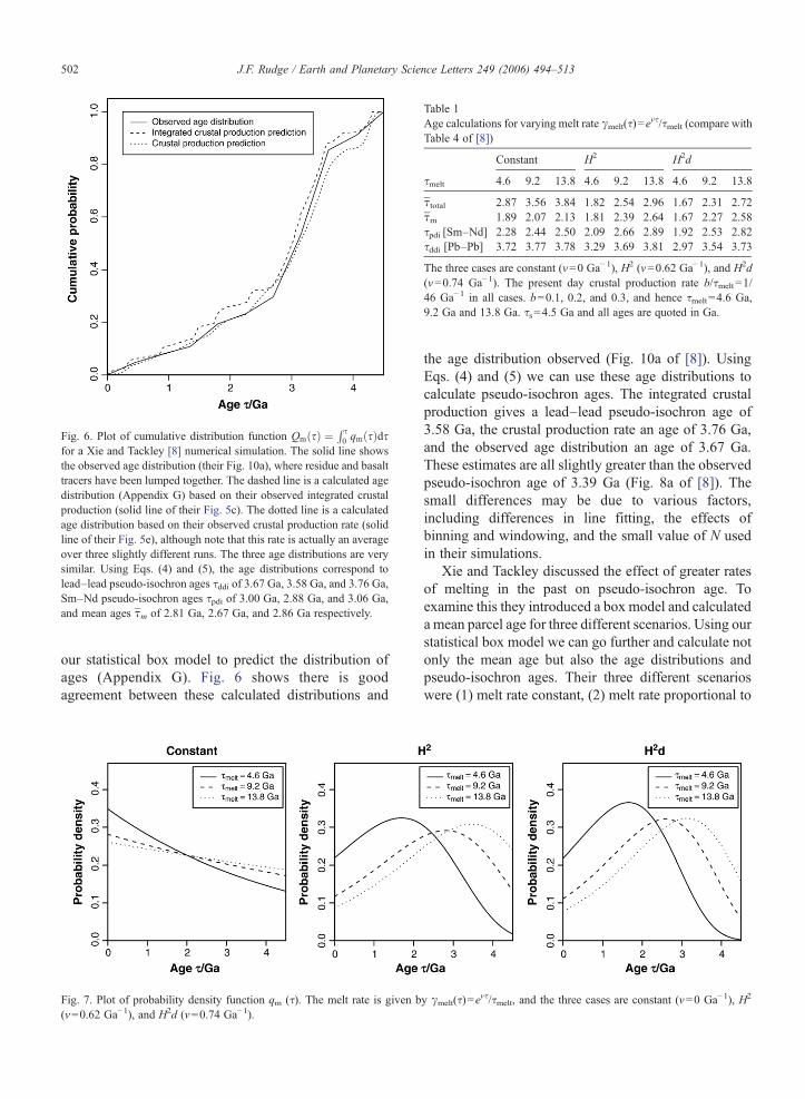
Fig. 6. Plot of cumulative distribution function QmðsÞ ¼R s0 qmðsÞds

for a Xie and Tackley [8] numerical simulation. The solid line showsthe observed age distribution (their Fig. 10a), where residue and basalttracers have been lumped together. The dashed line is a calculated agedistribution (Appendix G) based on their observed integrated crustalproduction (solid line of their Fig. 5c). The dotted line is a calculatedage distribution based on their observed crustal production rate (solidline of their Fig. 5e), although note that this rate is actually an averageover three slightly different runs. The three age distributions are verysimilar. Using Eqs. (4) and (5), the age distributions correspond tolead–lead pseudo-isochron ages τddi of 3.67 Ga, 3.58 Ga, and 3.76 Ga,Sm–Nd pseudo-isochron ages τpdi of 3.00 Ga, 2.88 Ga, and 3.06 Ga,and mean ages τm of 2.81 Ga, 2.67 Ga, and 2.86 Ga respectively.

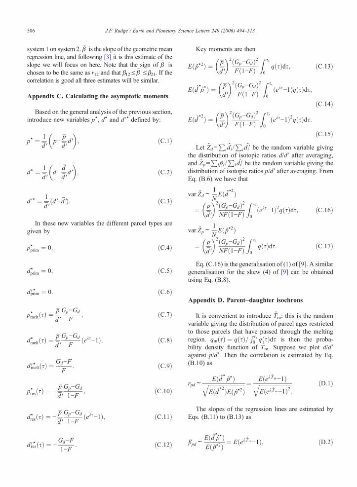
Table 1Age calculations for varying melt rate γmelt(τ)=e

ντ/τmelt (compare withTable 4 of [8])

Constant H2 H2d

τmelt 4.6 9.2 13.8 4.6 9.2 13.8 4.6 9.2 13.8

τtotal 2.87 3.56 3.84 1.82 2.54 2.96 1.67 2.31 2.72τm 1.89 2.07 2.13 1.81 2.39 2.64 1.67 2.27 2.58τpdi [Sm–Nd] 2.28 2.44 2.50 2.09 2.66 2.89 1.92 2.53 2.82τddi [Pb–Pb] 3.72 3.77 3.78 3.29 3.69 3.81 2.97 3.54 3.73

The three cases are constant (ν=0 Ga− 1), H2 (ν=0.62 Ga−1), and H2d(ν=0.74 Ga−1). The present day crustal production rate b/τmelt=1/46 Ga−1 in all cases. b=0.1, 0.2, and 0.3, and hence τmelt=4.6 Ga,9.2 Ga and 13.8 Ga. τs=4.5 Ga and all ages are quoted in Ga.


our statistical box model to predict the distribution ofages (Appendix G). Fig. 6 shows there is goodagreement between these calculated distributions and

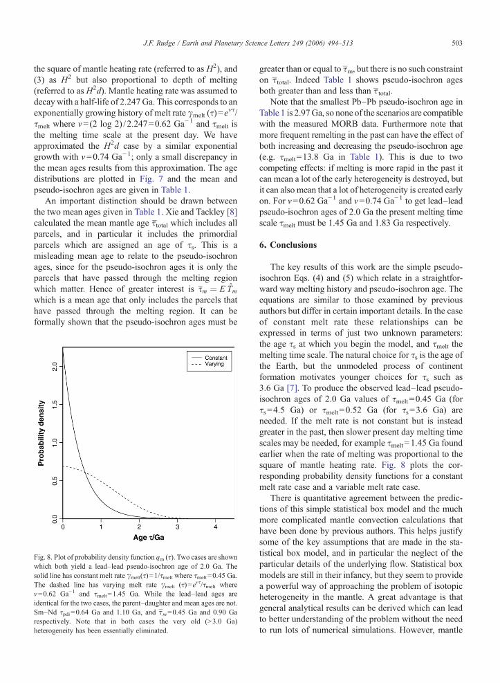
Fig. 7. Plot of probability density function qm (τ). The melt rate is given b(ν=0.62 Ga−1), and H2d (ν=0.74 Ga−1).

the age distribution observed (Fig. 10a of [8]). UsingEqs. (4) and (5) we can use these age distributions tocalculate pseudo-isochron ages. The integrated crustalproduction gives a lead–lead pseudo-isochron age of3.58 Ga, the crustal production rate an age of 3.76 Ga,and the observed age distribution an age of 3.67 Ga.These estimates are all slightly greater than the observedpseudo-isochron age of 3.39 Ga (Fig. 8a of [8]). Thesmall differences may be due to various factors,including differences in line fitting, the effects ofbinning and windowing, and the small value of N usedin their simulations.

Xie and Tackley discussed the effect of greater ratesof melting in the past on pseudo-isochron age. Toexamine this they introduced a box model and calculateda mean parcel age for three different scenarios. Using ourstatistical box model we can go further and calculate notonly the mean age but also the age distributions andpseudo-isochron ages. Their three different scenarioswere (1) melt rate constant, (2) melt rate proportional to

y γmelt(τ)=eντ/τmelt, and the three cases are constant (ν=0 Ga−1), H2


the square of mantle heating rate (referred to as H2), and(3) as H2 but also proportional to depth of melting(referred to as H2d). Mantle heating rate was assumed todecay with a half-life of 2.247 Ga. This corresponds to anexponentially growing history of melt rate γmelt (τ)=e

ντ/τmelt where ν=(2 log 2) /2.247=0.62 Ga−1 and τmelt isthe melting time scale at the present day. We haveapproximated the H2d case by a similar exponentialgrowth with ν=0.74 Ga−1; only a small discrepancy inthe mean ages results from this approximation. The agedistributions are plotted in Fig. 7 and the mean andpseudo-isochron ages are given in Table 1.

An important distinction should be drawn betweenthe two mean ages given in Table 1. Xie and Tackley [8]calculated the mean mantle age τtotal which includes allparcels, and in particular it includes the primordialparcels which are assigned an age of τs. This is amisleading mean age to relate to the pseudo-isochronages, since for the pseudo-isochron ages it is only theparcels that have passed through the melting regionwhich matter. Hence of greater interest is sm ¼ E Tm

which is a mean age that only includes the parcels thathave passed through the melting region. It can beformally shown that the pseudo-isochron ages must be

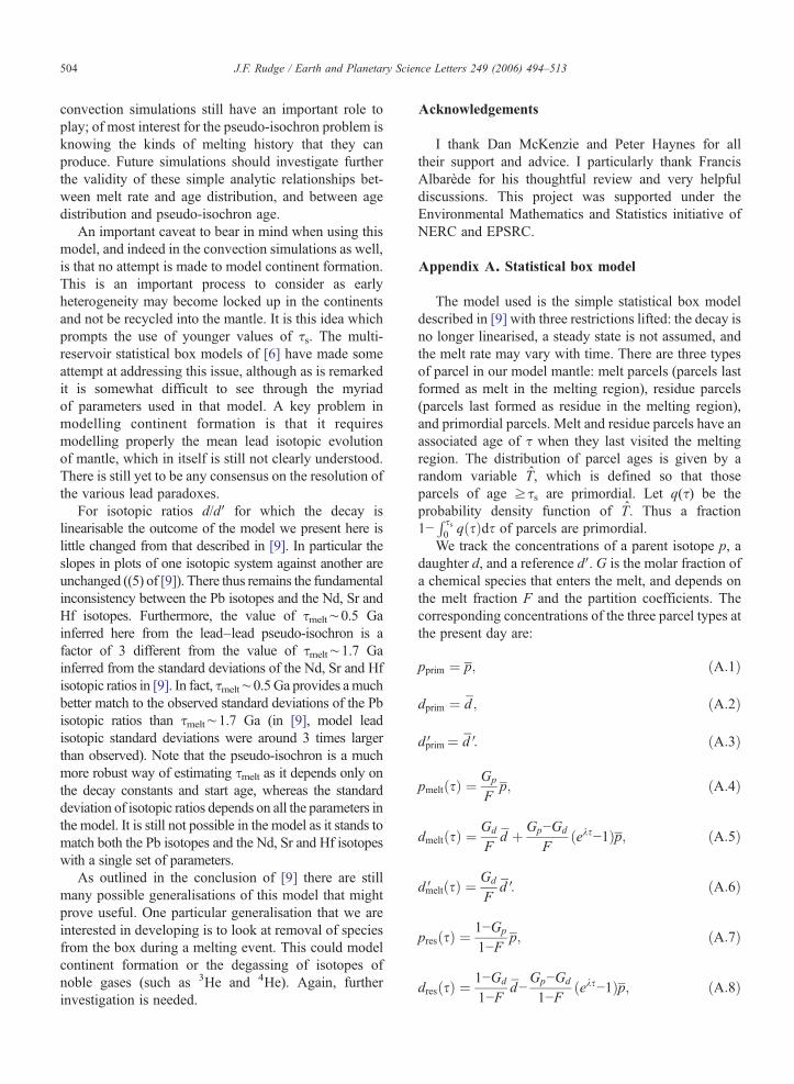
Fig. 8. Plot of probability density function qm (τ). Two cases are shownwhich both yield a lead–lead pseudo-isochron age of 2.0 Ga. Thesolid line has constant melt rate γmelt(τ)=1/τmelt where τmelt=0.45 Ga.The dashed line has varying melt rate γmelt (τ)=eντ/τmelt whereν=0.62 Ga−1 and τmelt=1.45 Ga. While the lead–lead ages areidentical for the two cases, the parent–daughter and mean ages are not.Sm–Nd τpdi=0.64 Ga and 1.10 Ga, and τm=0.45 Ga and 0.90 Garespectively. Note that in both cases the very old (N3.0 Ga)heterogeneity has been essentially eliminated.

greater than or equal to τm, but there is no such constrainton τ total. Indeed Table 1 shows pseudo-isochron agesboth greater than and less than τ total.

Note that the smallest Pb–Pb pseudo-isochron age inTable 1 is 2.97Ga, so none of the scenarios are compatiblewith the measured MORB data. Furthermore note thatmore frequent remelting in the past can have the effect ofboth increasing and decreasing the pseudo-isochron age(e.g. τmelt=13.8 Ga in Table 1). This is due to twocompeting effects: if melting is more rapid in the past itcan mean a lot of the early heterogeneity is destroyed, butit can also mean that a lot of heterogeneity is created earlyon. For ν=0.62 Ga−1 and ν=0.74 Ga−1 to get lead–leadpseudo-isochron ages of 2.0 Ga the present melting timescale τmelt must be 1.45 Ga and 1.83 Ga respectively.

6. Conclusions

The key results of this work are the simple pseudo-isochron Eqs. (4) and (5) which relate in a straightfor-ward way melting history and pseudo-isochron age. Theequations are similar to those examined by previousauthors but differ in certain important details. In the caseof constant melt rate these relationships can beexpressed in terms of just two unknown parameters:the age τs at which you begin the model, and τmelt themelting time scale. The natural choice for τs is the age ofthe Earth, but the unmodeled process of continentformation motivates younger choices for τs such as3.6 Ga [7]. To produce the observed lead–lead pseudo-isochron ages of 2.0 Ga values of τmelt=0.45 Ga (forτs=4.5 Ga) or τmelt=0.52 Ga (for τs=3.6 Ga) areneeded. If the melt rate is not constant but is insteadgreater in the past, then slower present day melting timescales may be needed, for example τmelt=1.45 Ga foundearlier when the rate of melting was proportional to thesquare of mantle heating rate. Fig. 8 plots the cor-responding probability density functions for a constantmelt rate case and a variable melt rate case.

There is quantitative agreement between the predic-tions of this simple statistical box model and the muchmore complicated mantle convection calculations thathave been done by previous authors. This helps justifysome of the key assumptions that are made in the sta-tistical box model, and in particular the neglect of theparticular details of the underlying flow. Statistical boxmodels are still in their infancy, but they seem to providea powerful way of approaching the problem of isotopicheterogeneity in the mantle. A great advantage is thatgeneral analytical results can be derived which can leadto better understanding of the problem without the needto run lots of numerical simulations. However, mantle


convection simulations still have an important role toplay; of most interest for the pseudo-isochron problem isknowing the kinds of melting history that they canproduce. Future simulations should investigate furtherthe validity of these simple analytic relationships bet-ween melt rate and age distribution, and between agedistribution and pseudo-isochron age.

An important caveat to bear in mind when using thismodel, and indeed in the convection simulations as well,is that no attempt is made to model continent formation.This is an important process to consider as earlyheterogeneity may become locked up in the continentsand not be recycled into the mantle. It is this idea whichprompts the use of younger values of τs. The multi-reservoir statistical box models of [6] have made someattempt at addressing this issue, although as is remarkedit is somewhat difficult to see through the myriadof parameters used in that model. A key problem inmodelling continent formation is that it requiresmodelling properly the mean lead isotopic evolutionof mantle, which in itself is still not clearly understood.There is still yet to be any consensus on the resolution ofthe various lead paradoxes.

For isotopic ratios d/d′ for which the decay islinearisable the outcome of the model we present here islittle changed from that described in [9]. In particular theslopes in plots of one isotopic system against another areunchanged ((5) of [9]). There thus remains the fundamentalinconsistency between the Pb isotopes and the Nd, Sr andHf isotopes. Furthermore, the value of τmelt∼0.5 Gainferred here from the lead–lead pseudo-isochron is afactor of 3 different from the value of τmelt∼1.7 Gainferred from the standard deviations of the Nd, Sr and Hfisotopic ratios in [9]. In fact, τmelt∼0.5Ga provides amuchbetter match to the observed standard deviations of the Pbisotopic ratios than τmelt∼1.7 Ga (in [9], model leadisotopic standard deviations were around 3 times largerthan observed). Note that the pseudo-isochron is a muchmore robust way of estimating τmelt as it depends only onthe decay constants and start age, whereas the standarddeviation of isotopic ratios depends on all the parameters inthe model. It is still not possible in the model as it stands tomatch both the Pb isotopes and the Nd, Sr and Hf isotopeswith a single set of parameters.

As outlined in the conclusion of [9] there are stillmany possible generalisations of this model that mightprove useful. One particular generalisation that we areinterested in developing is to look at removal of speciesfrom the box during a melting event. This could modelcontinent formation or the degassing of isotopes ofnoble gases (such as 3He and 4He). Again, furtherinvestigation is needed.

Acknowledgements

I thank Dan McKenzie and Peter Haynes for alltheir support and advice. I particularly thank FrancisAlbarède for his thoughtful review and very helpfuldiscussions. This project was supported under theEnvironmental Mathematics and Statistics initiative ofNERC and EPSRC.

Appendix A. Statistical box model

The model used is the simple statistical box modeldescribed in [9] with three restrictions lifted: the decay isno longer linearised, a steady state is not assumed, andthe melt rate may vary with time. There are three typesof parcel in our model mantle: melt parcels (parcels lastformed as melt in the melting region), residue parcels(parcels last formed as residue in the melting region),and primordial parcels. Melt and residue parcels have anassociated age of τ when they last visited the meltingregion. The distribution of parcel ages is given by arandom variable T, which is defined so that thoseparcels of age ≥τs are primordial. Let q(τ) be theprobability density function of T. Thus a fraction1−

R ss0 qðsÞds of parcels are primordial.

We track the concentrations of a parent isotope p, adaughter d, and a reference d′. G is the molar fraction ofa chemical species that enters the melt, and depends onthe melt fraction F and the partition coefficients. Thecorresponding concentrations of the three parcel types atthe present day are:

pprim ¼ p; ðA:1Þ

dprim ¼ d ; ðA:2Þ

dprimV ¼ d V: ðA:3Þ

pmeltðsÞ ¼ Gp

Fp; ðA:4Þ

dmeltðsÞ ¼ Gd

Fd þ Gp−Gd

Fðeks−1Þp; ðA:5Þ

dmeltV ðsÞ ¼ Gd

Fd V: ðA:6Þ

presðsÞ ¼ 1−Gp

1−Fp; ðA:7Þ

dresðsÞ ¼ 1−Gd

1−Fd−

Gp−Gd

1−Fðeks−1Þp; ðA:8Þ


dresV ðsÞ ¼ 1−Gd

1−Fd V; ðA:9Þ

where p, d , and d ′ are the mean concentrations of theisotopes in the box at the present day, and λ is the decayconstant.

Appendix B. The asymptotics of averaging ratioquantities

As before, we model sampling by taking a number Nof independent identically distributed (i.i.d.) samplesfrom our model mantle and averaging. Again, it isimportant to note that we are interested in ratioquantities. This section describes some importantgeneral results on the asymptotics of averaging ratioquantities.

Consider i.i.d. pairs of random variables {x i, ŷi},i=1, 2,…N. Suppose ŷiN0. We are interested in theasymptotic behaviour of the ratio of sums

Z ¼Xi

xi =Xi

yi ðB:1Þ

for N large. Let

x⋆ ¼ 1y

x−xyy

� �; ðB:2Þ

y⋆ ¼ 1yð y−yÞ; ðB:3Þ

where x ¼ EðxÞ; y ¼ Eð yÞ. Note that Eðx⋆Þ ¼ Eðy⋆Þ ¼0. Note also that

Z ¼P

xiPyi¼ x

yþ

Px⋆i =N

1þPy⋆i =N

: ðB:4Þ

It can be shown [17] that Z is asymptotically normalfor large N under appropriate assumptions (assumptionswhich give the central limit theorem for

Px⋆i and give

the law of large numbers forP

y⋆i ). The condition ŷiN0ensures that moments of Z are well defined, and Cauchydistribution problems do not arise. By Taylor expanding(B.4) and taking expectations the following expressionsfor the asymptotic moments can be derived:

l ¼ Z ¼ EðZ Þ ¼ xy−1NEðx⋆ y⋆Þ þ O

1N2

� �; ðB:5Þ

l2 ¼ r2 ¼ EðZ −ZÞ2 ¼ 1NEðx⋆2Þ þ O

1N2

� �; ðB:6Þ

l3 ¼ EðZ−ZÞ3 ¼ 1N2

ðEðx⋆3Þ−6Eðx⋆ y⋆ÞEðx⋆2ÞÞ

þ O1N3

� �: ðB:7Þ

Hence the skew parameter γ1 is

g1 ¼l3

ðl2Þ3=2¼ Eðx⋆3Þ−6Eðx⋆ y⋆ÞEðx⋆2Þ

N1=2ðEðx⋆2ÞÞ3=2

þ O1

N3=2

� �: ðB:8Þ

The kurtosis and higher order moments can bederived similarly by expanding to higher orders.

In this work we are most concerned with plots of oneratio against another. So consider two sets of i.i.d. pairsof random variables {xi, ŷi}1 and {xi, ŷi}2, i=1, 2,…N.Then the covariance of Z1 and Z2 is given by

covðZ1; Z2Þ ¼ EððZ1−Z 1ÞðZ2−Z 2ÞÞ

¼ 1NEðx⋆1 x⋆2Þ þ O

1N 2

� �

¼ 1Ncovðx⋆1; x⋆2Þ þ O

1N 2

� �;

ðB:9Þ

with corresponding correlation

r12 ¼ corðZ1; Z2Þ ¼ covðZ1; Z2Þr1r2

¼ Eðx⋆1 x⋆2ÞffiffiffiffiffiffiffiffiffiffiffiffiffiffiffiffiffiffiffiffiffiffiffiffiffiEðx⋆21 ÞEðx⋆22 Þ

q

þO1N

� �¼ corðx⋆1; x⋆2Þ þ O

1N

� �: ðB:10Þ

We are most interested in calculating the slope of aregression line of one system against another. There aremany different methods for fitting regression lines to acloud of data pointswhichmake various assumptions aboutthe underlying data. Three commonly used estimates are

b12 ¼ r12r2r1

¼ Eðx⋆1 x⋆2ÞEðx⋆21 Þ þ O

1N

� �; ðB:11Þ

b ¼ r2r1

¼ffiffiffiffiffiffiffiffiffiffiffiffiffiEðx⋆22 ÞEðx⋆21 Þ

sþO

1N

� �; ðB:12Þ

b21 ¼1r12

r2r1

¼ Eðx⋆22 ÞEðx⋆1 x⋆2Þ

þ O1N

� �; ðB:13Þ

where β12 is the slope of the linear least squares regressionline of system 2 on system 1, and β21 is the same line but for

Eð p Þ


system 1 on system 2. β is the slope of the geometric meanregression line, and following [3] it is this estimate of theslope we will focus on here. Note that the sign of β ischosen to be the same as r12 and that β12≤ β ≤β21. If thecorrelation is good all three estimates will be similar.

Appendix C. Calculating the asymptotic moments

Based on the general analysis of the previous section,introduce new variables p⋆, d⋆ and d′⋆ defined by:

p⋆ ¼ 1

d Vp−

p

d Vd V

� �; ðC:1Þ

d⋆ ¼ 1

d Vd−

d

d Vd V

� �; ðC:2Þ

d V⋆ ¼ 1

d Vðd V−d VÞ: ðC:3Þ

In these new variables the different parcel types aregiven by

p⋆prim ¼ 0; ðC:4Þ

d⋆prim ¼ 0; ðC:5Þ

d V⋆prim ¼ 0: ðC:6Þ

p⋆meltðsÞ ¼p

d VGp−Gd

F; ðC:7Þ

d⋆meltðsÞ ¼p

d VGp−Gd

Fðeks−1Þ; ðC:8Þ

d V⋆meltðsÞ ¼ Gd−FF

: ðC:9Þ

p⋆resðsÞ ¼ −p

d VGp−Gd

1−F; ðC:10Þ

d⋆resðsÞ ¼ −p

d VGp−Gd

1−Fðeks−1Þ; ðC:11Þ

d V⋆resðsÞ ¼ −Gd−F1−F

: ðC:12Þ

Key moments are then

Eð p⋆2Þ ¼ p

d V

� �2ðGp−GdÞ2Fð1−FÞ

Z ss

0qðsÞds; ðC:13Þ

Eðd ⋆p⋆Þ ¼ p

d V


Z ss

0ðeks−1ÞqðsÞds;

ðC:14Þ

Eðd ⋆2Þ ¼ p

d V


Z ss

0ðeks−1Þ2qðsÞds:

ðC:15ÞLet Zd=

Pi di /

Pi di′ be the random variable giving

the distribution of isotopic ratios d/d′ after averaging,and Zp=

Pi pi /

Pi di′ be the random variable giving the

distribution of isotopic ratios p/d′ after averaging. FromEq. (B.6) we have that

var Zdf1NEðd ⋆2Þ

¼ p

d V

� �2ðGp−GdÞ2NFð1−FÞ

Z ss

0ðeks−1Þ2qðsÞds; ðC:16Þ

var Zpf1NEð p⋆2Þ

¼ p

d V

� �2ðGp−GdÞ2NFð1−FÞ

Z ss

0qðsÞds: ðC:17Þ

Eq. (C.16) is the generalisation of (1) of [9]. A similargeneralisation for the skew (4) of [9] can be obtainedusing Eq. (B.8).

Appendix D. Parent–daughter isochrons

It is convenient to introduce Tm: this is the randomvariable giving the distribution of parcel ages restrictedto those parcels that have passed through the meltingregion. qmðsÞ ¼ qðsÞ= R ss

0 qðsÞds is then the proba-bility density function of Tm. Suppose we plot d/d′against p/d′. Then the correlation is estimated by Eq.(B.10) as

rpdfEðd ⋆

p⋆ÞffiffiffiffiffiffiffiffiffiffiffiffiffiffiffiffiffiffiffiffiffiffiffiffiffiffiffiEðd ⋆2ÞEð p⋆2Þ

q ¼ Eðek Tm−1ÞffiffiffiffiffiffiffiffiffiffiffiffiffiffiffiffiffiffiffiffiffiffiffiEðek Tm−1Þ2

q:

ðD:1Þ

The slopes of the regression lines are estimated byEqs. (B.11) to (B.13) as

bpdfEðd ⋆

p⋆Þ⋆2 ¼ Eðek Tm−1Þ; ðD:2Þ


bf

ffiffiffiffiffiffiffiffiffiffiffiffiffiffiEðd ⋆2ÞEð p⋆2Þ

s¼

ffiffiffiffiffiffiffiffiffiffiffiffiffiffiffiffiffiffiffiffiffiffiffiffiEðek Tm−1Þ2;

qðD:3Þ

bdpfEðd ⋆2ÞEðd ⋆

p⋆Þ¼ Eðek Tm−1Þ2

Eðek Tm−1Þ: ðD:4Þ

The parent–daughter pseudo-isochron age is relatedto the slope of the regression line by

ekspdi−1 ¼ b; ðD:5Þand thus using the geometric mean regression line (D.3)the model parent–daughter pseudo-isochron equation is

ðekspdi−1Þ2 ¼ Eðek Tm−1Þ2: ðD:6Þ

Note that when the decay is linearisable ( Tm≪1/λ)Eqs. (D.1) and (D.6) reduce to rpd ¼ ETm=

ffiffiffiffiffiffiffiffiffiET

2m

qand

spdi ¼ffiffiffiffiffiffiffiffiffiffiffiE T

2m

q.

Appendix E. Daughter–daughter isochrons

Now suppose we plot (d/d′)2 against (d/d′)1 for twodifferent isotopic systems 1 and 2. Key moments arethen

Eðd ⋆21 Þ ¼ p1

d V1

� �2ðGp1−Gd1Þ2Fð1−FÞ

Z ss

0ðek1s−1Þ2qðsÞds;

ðE:1Þ

Eðd ⋆1 d

⋆2Þ ¼

p1d V1

� �p2d V2

� � ðGp1−Gd1ÞðGp2−Gd2ÞFð1−FÞ

�Z ss

0ðek1s−1Þðek2s−1ÞqðsÞds; ðE:2Þ

Eðd ⋆22 Þ ¼ p2

d V2

� �2ðGp2−Gd2Þ2Fð1−FÞ

Z ss

0ðek2s−1Þ2qðsÞds:

ðE:3ÞThe correlation is then given by

r12fEðek1 Tm−1Þðek2 Tm−1ÞffiffiffiffiffiffiffiffiffiffiffiffiffiffiffiffiffiffiffiffiffiffiffiffiffiffiffiffiffiffiffiffiffiffiffiffiffiffiffiffiffiffiffiffiffiffiffiffiffiEðek1 Tm−1Þ2Eðek2 Tm−1Þ2

q� sgnððGp1−Gd1ÞðGp2−Gd2ÞÞ:

Note that |r12|∼1 if the decay is linearisable ( Tm≪1/λ1 and 1/λ2), which is why in Fig. 4 of [9] the model data

form almost perfect straight lines. However, when thedecay is not linearisable we will not get perfectcorrelation. The slope of the geometric mean regressionline is given by

bfð p2=d V2ÞðGp2−Gd2Þð p1=d V1 ÞðGp1−Gd1Þ

ffiffiffiffiffiffiffiffiffiffiffiffiffiffiffiffiffiffiffiffiffiffiffiffiffiffiEðek2 Tm−1Þ2Eðek1 Tm−1Þ2

:

vuut ðE:5Þ

Note that if the decay is linearisable this reduces to

bfð p2=d V2ÞðGp2−Gd2Þk2ð p1=d V1ÞðGp1−Gd1Þk1

; ðE:6Þ

which is precisely (5) of [9]. Eq. (E.5) is thegeneralisation of (5) of [9]. Hence for those isotopicsystems for which a linear decay approximation is validthe slopes are unchanged from [9].

We are particularly interested in a special case of Eq.(E.5). If the parent and daughter elements are the same,and the reference isotope is also the same, then Eq. (E.5)reduces to

bfp2p1

ffiffiffiffiffiffiffiffiffiffiffiffiffiffiffiffiffiffiffiffiffiffiffiffiffiffiEðek2 Tm−1Þ2Eðek1 Tm−1Þ2

:

vuut ðE:7Þ

This is the generalisation of (6) of [9]. The otherestimates of the slope of the regression line in thisspecial case are given by

b12 fp2p1

dEðek1 Tm−1Þðek2 Tm−1Þ

Eðek1 Tm−1Þ2;

b21fp2p1

dEðek2 Tm−1Þ2

Eðek1 Tm−1Þðek2 Tm−1Þ:

ðE:8Þ

The daughter–daughter pseudo-isochron age isrelated to the slope of the regression lines by

p2p1

dek2sddi−1ek1sddi−1

¼ b: ðE:9Þ

Hence, combining Eqs. (E.7) and (E.9) the modelpseudo-isochron age τddi satisfies the simple relationship


Eðek2 Tm−1Þ2Eðek1 Tm−1Þ2

: ðE:10Þ

Note that when the decay is linearisable ( Tm≪1/λ1and 1/λ2) Eq. (E.10) reduces to sddi ¼ E T

3m =E T

2m (by

Taylor series expansion).


Appendix F. Means

It is important to distinguish between differentdefinitions of the mean age of parcels. Since the hetero-geneity we are interested in is generated by fractionationon melting, an important mean age is sm ¼ ETm, themean age of the parcels that have passed through themelting region. Primordial parcels do not contribute tothe pseudo-isochron ages. The mean mantle age τtotal isoften defined by including the primordial parcels andassigning them an age of τs, and it is this definition that isused in [8]. Hence τtotal≥ τm. We have

stotal ¼Z ss

0sqðsÞdsþ ss 1−

Z ss

0qðsÞds

� �; ðF:1Þ

sm ¼ ETm ¼Z ss

0sqmðsÞds: ðF:2Þ

The parent–daughter pseudo-isochron age τpdi is anexample of a generalised mean [13]. A generalised meanMϕ is defined by M/ðX Þ ¼ /−1ðE/ðX ÞÞ, where ϕ is astrictly monotonic function, and X is a random variable.Commonly encountered examples include ϕ(x)=x (arith-metic mean), ϕ(x)=xr (power mean), and ϕ(x)= log x(geometric mean). In the case of the parent–daughterpseudo-isochron Eq. (D.6), ϕ(x)=(eλx−1)2. Generalisedmeans have a number of important properties, but of mostinterest to us is the notion of ‘comparability’: whetherthere is always an inequality between different meansregardless of the distribution of the random variable X. Acommon example of comparability is the arithmeticmean–geometric mean inequality. There is an importanttheorem which states that if ψ and χ are monotonicallyincreasing functions, ϕ=χψ−1, and ϕ″N0, thenMψ≤Mϕ

(Theorem 96 of [13]). By use of this theorem we findthe following inequalities are satisfied by the parent–daughter pseudo-isochron age:

min TmVsmVffiffiffiffiffiffiffiffiET

2m

qVspdiðk1ÞVspdiðk2ÞVmax Tm;

ðF:3Þwhere 0bλ1bλ2, and min Tm and max Tm are thesmallest and largest ages respectively with any proba-bility mass.

The daughter–daughter pseudo-isochron age τddi isnot a generalised mean as described by [13], but it is anexample of a generalised abstracted mean (Definition2.4 of [14]). A generalised abstracted mean is defined byM/1;/2

ðX Þ ¼ ð/1=/2Þ−1ðE/1ðX Þ=E/2ðX ÞÞ where ϕ1/ϕ2 is a strictly monotonic function. In the case of thedaughter–daughter pseudo-isochron Eq. (E.10), ϕ1(x)=(eλ1x−1)2 and ϕ2(x)= (e

λ2x−1)2. The generalised ab-

stracted mean shares many of the properties of thegeneralised mean of [13], and under a suitable trans-formation of the probability density function can bewritten in the same form. However, for our purposeswhat is of most interest is the inequality

spdiðk2Þ V sddiðk1; k2Þ VmaxTm: ðF:4Þ

The above inequalities (F.3) and (F.4) are strictinequalities unless all the probability mass is concen-trated at a single age. In this case all the inequalities areequalities, and all the means yield this single age.

Appendix G. Relating melt rate and parcel ages

Suppose melt rate as a function of age τ is γmelt(τ).Define τmelt to be the melting time scale at the presentday, so that γmelt(0)=1/τmelt. Let QðsÞ ¼ PðTVsÞ be theproportion of material in the box with age less than τ(the cumulative distribution function), with 1−Q(τs)being the proportion of primordial material. Q(τ)satisfies

dQðsÞds

¼ gmeltðsÞð1−QðsÞÞ; Qð0Þ ¼ 0; ðG:1Þ

and thus

QðsÞ ¼ 1−exp −Z s

0gmeltðsÞds

� �: ðG:2Þ

Hence the probability density functions are

qðsÞ ¼ dQðsÞds

¼ gmeltðsÞexp −Z s

0gmeltðsÞds

� �; ðG:3Þ

qmðsÞ ¼ qðsÞQðssÞ ¼

1QðssÞ

dQðsÞds

: ðG:4Þ

In some cases it is more convenient to work with thecumulative distribution function (cdf) rather than thepdf. Note that if f (0)=0 (as it is for all functions weconsider) then

Ef ð TmÞ ¼Z ss

0f VðsÞð1−QmðsÞÞds; ðG:5Þ

where the cdf Qm(τ) is given by

QmðsÞ ¼Z s

0qmðsÞds ¼ QðsÞ

QðssÞ : ðG:6Þ

Xie and Tackley [8] quote results from theirnumerical simulations in terms of the crustal production


rate given by bγmelt(τ), where b is their basalt fraction(b=0.3 in their standard runs). Their integrated crustalproduction (integrated forward in time) is given as afunction of age by

cðsÞ ¼ 1−exp −Z ss

sbgmeltðsÞds

� �; ðG:7Þ

which implies

exp −Z s

0gmeltðsÞds

� �¼ 1−cð0Þ

1−cðsÞ� �1=b

: ðG:8Þ

Hence the cdf Qm (τ) (and thus also pseudo-isochronages) can be calculated directly from their integratedcrustal production or their crustal production rate.

For a constant melt rate γmelt(τ)=1/τmelt and T is anexponential random variable with parameter 1/τmelt. Thecorresponding probability density functions are

qðsÞ ¼ e−s=smelt=smelt; ðG:9Þ

qmðsÞ ¼ e−s=smelt=ðsmeltð1−e−ss=smeltÞÞ; ðG:10Þ

and corresponding means are

stotal ¼ smeltð1−e−ss=smeltÞ; ðG:11Þ

sm ¼ ETm ¼ smelt1−e−ss=smeltð1þ ss=smeltÞ

1−e−ss=smelt; ðG:12Þ


2m

q¼

ffiffiffi2

psmelt

ffiffiffiffiffiffiffiffiffiffiffiffiffiffiffiffiffiffiffiffiffiffiffiffiffiffiffiffiffiffiffiffiffiffiffiffiffiffiffiffiffiffiffiffiffiffiffiffiffiffiffiffiffiffiffiffiffiffiffiffiffiffiffiffiffiffiffiffiffiffiffiffiffiffiffiffiffiffi1−e−ss=smelt 1þ ss=smelt þ 1

2 ðss=smeltÞ2� �

1−e−ss=smelt:

vuutðG:13Þ

Appendix H. Constant melt rate: Parent–daughterisochrons

For constant melt rate the parent–daughter pseudo-isochron equation is

ðekspdi−1Þ2 ¼R ss0 ðeks−1Þ2e−s=smelt ds

smeltð1−e−ss=smeltÞ : ðH:1Þ

To gain some insight into the behaviour of thisequation we now consider some simple asymptotics.

H.1. Asymptotics when τmelt or τs≪1/λ

Since we often study slowly decaying isotopes, themost important asymptotics are when τmelt or τs≪1/λ.In this limit the correlation becomes

rpd ¼ 1−e−ss=smeltð1þ ss=smeltÞffiffiffiffiffiffiffiffiffiffiffiffiffiffiffiffiffiffiffiffiffiffiffiffiffiffiffiffiffiffiffiffiffiffiffiffiffiffiffiffiffiffiffiffiffiffiffiffiffiffiffiffiffiffiffiffiffiffiffiffiffiffiffiffiffiffiffiffiffiffiffiffiffiffiffiffiffiffiffiffiffiffiffiffiffiffiffiffiffiffiffiffiffiffiffiffiffiffiffiffiffiffiffiffiffiffiffiffi2ð1−e−ss=smeltÞ 1−e−ss=smelt 1þ ss=smelt þ 1

2 ðss=smeltÞ2� �� r

:

ðH:2ÞFurthermore, if τs/τmelt≫1 then rpdf1=

ffiffiffi2

pc0:71.

Alternatively if τs/τmelt≪1 then rpdfffiffiffi3

p=2c0:87. For

linearisable decay rpd always lies between these twovalues. It is important to note that there is thus never aperfect correlation between d/d′ and p/d′.

When τmelt or τs≪1/λ the parent–daughterpseudo-isochron age becomes simply spdi ¼


2m

q,

which is given for constant melt rate by Eq. (G.13).If τs/τmelt≫1 Eq. (G.13) simplifies to spdif

ffiffiffi2

psmelt,

which determines the slope of curves near the originin Figs. 3b and 4b, and the asymptotes for large τs inFig. 3a. On the other hand, if τs/τmelt≪1 Eq. (G.13)simplifies to spdifss=

ffiffiffi3

p, which determines the slope

of curves near the origin in Figs. 3a and 4a, and theasymptotes for large τmelt in Fig. 3b.

H.2. Asymptotics when τs≪τmelt

When the decay is not linearisable, asymptoticsbased solely on τs≪τmelt can be found. The pseudo-isochron Eq. (H.1) becomes

ðekspdi−1Þ2 ¼ 2kss þ 3−4ekss þ e2kss

2kss; ðH:3Þ

which is independent of τmelt. This equation determinesthe τmelt=∞ Ga curve in Figs. 3a and 4a, and asymptotesfor large τmelt in Figs. 3b and 4b.

H.3. Asymptotics when τs≫τmelt

Eq. (H.1) has two regimes of asymptotic behaviourwhen τs/τmelt≫1. If λτmeltN1/2 then

e2kspdi ¼ eð2ksmelt−1Þss=smelt

2ksmelt−1; ðH:4Þ

whereas if λτmeltb1/2 then

ðekspdi−1Þ2 ¼ 2ðksmeltÞ2ð1−ksmeltÞð1−2ksmeltÞ : ðH:5Þ


Note that Eq. (H.4) depends on τs whereas Eq. (H.5)is independent of τs. This is why in Fig. 4a curves withτmeltb1/2λ flatten out for large τs, while curves withτmeltsN1/2λ grow linearly for large τs with slope 1−1/2λτmelt.

Appendix I. Constant melt rate:Daughter–daughter isochrons

The constant melt rate daughter–daughter pseudo-isochron equation is


R ss0 ðek2s−1Þ2e−s=smeltdsR ss0 ðek1s−1Þ2e−s=smeltds

: ðI:1Þ

Again, insights into the behaviour of Eq. (I.1) can begained by some simple asymptotics, although linearis-ing the decay is not as relevant here. We will assumewithout loss of generality that λ2Nλ1 for the subsequentasymptotics.

I.1. Asymptotics when τs≪τmelt

When τs≪ τmelt the pseudo-isochron Eq. (I.1)becomes


k1k2

d2k2ss þ 3−4ek2ss þ e2k2ss

2k1ss þ 3−4ek1ss þ e2k1ss: ðI:2Þ

Note that this equation is independent of τmelt. Thisequation determines the asymptotes for large τmelt inFig. 5b, and the τmelt =∞ Ga curve in Fig. 5a.Furthermore, if it is also the case that λτs≪1, we canTaylor expand both sides to find

k22k21

ð1þ ðk2−k1Þsddi þ N Þ

¼ k22k21

1þ 3ðk2−k1Þ4

ss þ N� �

; ðI:3Þ

and thus get the simple result that sddif 34 ss, which

determines the slope of curves near the origin in Fig. 5a.If instead λτs≫1 then we can approximate both sidesas

e2ðk2−k1Þsddi ¼ k1k2

e2ðk2−k1Þss ; ðI:4Þ

which demonstrates that the slope of the τmelt=∞ Gacurve in Fig. 5a will approach 1 for large τs.

I.2. Asymptotics when τs≫τmeltWe have three different regimes of asymptotic

behaviour for Eq. (I.1) when τs≫τmelt. If τmeltN1/2λ1the pseudo-isochron equation is

e2ðk2−k1Þsddi ¼ e2ðk2−k1Þss2k1smelt−12k2smelt−1

; ðI:5Þ

if 1/2λ2bτmeltb1/2λ1 then

e2ðk2−k1Þsddi

¼ eð2k2smelt−1Þss=smeltð1−k1smeltÞð1−2k1smeltÞðk1smeltÞ2ð2k2smelt−1Þ

; ðI:6Þ

and if τmeltb1/2λ2 then


k22ð1−k1smeltÞð1−2k1smeltÞk21ð1−k2smeltÞð1−2k2smeltÞ

: ðI:7Þ

The most important feature of Eq. (I.7) is that it isindependent of τs, whereas in the other two asymptoticregimes there is a dependence on τs. This is why forvalues of τmeltb1/2λ2 in Fig. 5a the curve flattens outfor large τs whereas in the other regimes they growlinearly for large τs with slopes (λ2−1/2τmelt) / (λ2−λ1)and 1 respectively. Eq. (I.7) can be further simplified ifλτmelt≪1. Both sides can be Taylor expanded to yield

k22k21

ð1þ ðk2−k1Þsddi þ N Þ

¼ k22k21

ð1þ 3ðk2−k1Þsmelt þ N Þ; ðI:8Þ

leading to the simple result that τddi∼3τmelt, whichdetermines the slope of curves near the origin in Fig. 5b.

Appendix J. Relationship to linear evolution models

There is an important connection between ourstatistical box model and the pseudo-isochron equationsderived from linear evolution models by previousauthors [3,4,5]. Suppose we divide the box into twobased on parcel type. Let all the residue parcels and afraction 1−F of the primordial parcels be called reservoir1, and all the melt parcels and a fraction F of theprimordial parcels be reservoir 2. These two reservoirsdo not change in size over time. Reservoir 1 is a fraction1−F of the box, and reservoir 2 a fraction F. At an age τsbefore the present all parcels are primordial and thus bothreservoirs have the same uniform isotopic concentra-tions. The mean concentrations of p, d and d′ at thepresent in each reservoir can be calculated by integratingEqs. (A.1) to (A.9) over the age distribution of parcels.


For the isochron calculation it is simplest to considerinstead the p⋆ and d⋆ values. Let p1

⋆ be the randomvariable giving the distribution of p⋆ in reservoir 1, andd 1⋆, p2

⋆ and d 2⋆

be defined similarly. Note that thesubscripts 1 and 2 now refer to the different reservoirs,rather than the different isotopic systems as in earliersections. Integration of Eqs. (C.4) to (C.12) yields themean values as

E p⋆1 ¼ −p

d VGp−Gd

1−F

Z ss

0qðsÞds; ðJ:1Þ

E d⋆1 ¼ −

p

d VGp−Gd

1−F

Z ss

0ðeks−1ÞqðsÞds; ðJ:2Þ

E p⋆2 ¼p

d VGp−Gd

F

Z ss

0qðsÞds; ðJ:3Þ

E d⋆2 ¼

p

d VGp−Gd

F

Z ss

0ðeks−1ÞqðsÞds: ðJ:4Þ

By multiplying these expressions by the fraction ofthe box each reservoir occupies these can be convertedinto molar values n⋆ and m⋆ (Eqs. (21) and (22)) as

n⋆1 ¼ ð1−FÞE p⋆1 ¼ −p

d VðGp−GdÞ

Z ss

0qðsÞds; ðJ:5Þ

m⋆1 ¼ ð1−FÞE d

⋆1

¼ −p

d VðGp−GdÞ

Z ss

0ðeks−1ÞqðsÞds: ðJ:6Þ

where n2⋆=−n1⋆ and m2

⋆=−m1⋆. Eqs. (J.5) and (J.6) are

solutions of Eqs. (25) and (26), and are the backwardin time versions of (A1–4) and (A1–5) of [3] withΔ⟨α⟩= 0. The number of moles of each isotopespecies in the two reservoirs must be modelled by thelinear evolution Eqs. (10)–(15); the only question isfinding expressions for the residence times. Here therelaxation times for parent and daughter are bothgiven by 1/γmelt, since they are both fractionated bythe same melting process on the same timescale. Theindividual residence times for each reservoir aredetermined by the fraction of moles G that enter themelt for each chemical species as

s1 ¼ 1Gpgmelt

; s2 ¼ 1ð1−GpÞgmelt

; ðJ:7Þ

h1 ¼ 1Gdg

; h2 ¼ 1ð1−GdÞg : ðJ:8Þ

melt melt

Consider a pseudo-isochron defined where the tworeservoirs and the whole box lie on the isochrondiagram. The slope in the parent–daughter isochrondiagram is given by

ðm=sÞ1−ðm=sÞ1þ2

ðn=sÞ1−ðn=sÞ1þ2

¼ m⋆1

n⋆1¼

R ss0 ðeks−1ÞqðsÞdsR ss

0 qðsÞds¼ Eðek Tm−1Þ:

ðJ:9Þ

Hence the corresponding pseudo-isochron equationsare

ekspdil−1 ¼ Eðek Tm−1Þ; ðJ:10Þ


¼ Eðek2 Tm−1ÞEðek1 Tm−1Þ

; ðJ:11Þ

which are just Eqs. (D.6) and (E.10) with squaredsremoved, and hence we will refer to these as the linearpseudo-isochron equations.

An alternative reservoir representation is to considerthe box split into three reservoirs, one with all the meltparcels, one with all the residue parcels, and one withall the primordial parcels. These three reservoirschange in size over time, with the melt and residuereservoirs growing at the expense of the primordialreservoir. This is analogous to model I of Jacobsen andWasserburg [18] where their depleted mantle reservoir2 and crust reservoir 3 grow from a homogenousundepleted mantle reservoir 1. Compare the statisticalbox model result, obtained by integrating Eqs. (A.4) to(A.9),

E d res

E d resV−d

d V¼ −

p

d VGp−Gd

1−GdEðek Tm−1Þ; ðJ:12Þ

E dmelt

E dmeltV−d

d V¼ p

d VGp−Gd

GdEðek Tm−1Þ; ðJ:13Þ

with (19) of [18], rewritten using an integration byparts,

Nd;jðsÞNs;jðsÞ −

Nd;1ðsÞNs;1ðsÞ

¼ Nr;1ðsÞNs;1ðsÞ f

r=sj

Z s

0ðekðs−nÞ−1Þ 1

MjðsÞdMjðnÞdn

dn:

ðJ:14ÞEqs. (J.12) and (J.13) are equivalent to Eq. (J.14),

although note that Eq. (J.14) is written with τ running


forward in time. The fractionation factors relate through1 + f2 = (1− Gp) / (1−Gd) and 1 + f3 = Gp/Gd. Thecorresponding probability density function of parcelsages is (1 /Mj(τ))dMj(ξ) / dξ (compare with Eq. (G.4)).Note that the relationship between melt rate and agedistribution will be slightly different between the twomodels, since there is recycling in the statistical boxmodel (a melt parcel may become a residue parcel andviceversa), but not in model I. The pseudo-isochronequations that result from where the three reservoirsplot on the isochron diagram are also Eqs. (J.10) and(J.11).

The linear parent–daughter pseudo-isochron age τpdilis also an example of a generalised mean, with ϕ(x)=eλx−1. The linear pseudo-isochron ages satisfy

min Tm V smVspdilðk1ÞVspdilðk2ÞVsddilðk1; k2ÞVmax Tm ;

ðJ:15Þ

where 0bλ1bλ2. For linearisable decay (Tm≪1/λ) thelinear parent–daughter pseudo-isochron Eq. (J.10)reduces to τpdil =ETm= τm, and the linear daughter–daughter pseudo-isochron Eq. (J.11) to τddil =ETm/ETm.It can be shown that the linear ages are always less thanthe corresponding quadratic ages, namely that τpdil(λ)≤τpdil(λ), and τddi(λ1, λ2)≤τddi(λ1, λ2).

For the case of constant melt rate the linear parent–daughter pseudo-isochron equation is

ekspdil−1 ¼R ss0 ðeks−1Þe−s=smelt ds

smeltð1−e−ss=smeltÞ¼ ksmelt þ ð1−ksmeltÞe−ss=smelt−eðksmelt−1Þss=smelt

ð1−ksmeltÞð1−e−ss=smeltÞ ;

ðJ:16Þ

which is the parent–daughter pseudo-isochron Eq. (A2–4) of [3]. This should be compared with our Eq. (H.1).The corresponding linear daughter–daughter pseudo-isochron equation is


¼R ss0 ðek2s−1Þe−s=smelt dsR ss0 ðek1s−1Þe−s=smelt ds

¼ 1−k1smelt

1−k2smelt

� ð1−k2smeltÞe−ss=smelt þ k2smelt−eðk2smelt−1Þss=smelt

ð1−k1smeltÞe−ss=smelt þ k1smelt−eðk1smelt−1Þss=smelt;

ðJ:17Þ

which is precisely the daughter–daughter pseudo-isochron Eq. (A2–9) of [3]. This should be compared

with our Eq. (I.1). Furthermore, when τmelt≪τs andλτmeltb1 Eqs. (J.16) and (J.17) become

ekspdil−1 ¼ ksmelt

1−ksmeltZspdil ¼ −

1klogð1−ksmeltÞ; ðJ:18Þ


¼ k2ð1−k1smeltÞk1ð1−k2smeltÞ ; ðJ:19Þ

which are the pseudo-isochron Eqs. (A2–6) and (A2–10) of [3], (31) and (32) of [4], and (7) and (9) of [5].The corresponding equations in our model are (H.5) and(I.7). The τmelt≪τs and λτmeltb1 limit is precisely thesame as the conditions for secular equilibrium in [4] and[5]. [3] explores various other asymptotic regimes forEqs. (J.16) and (J.17), as we have for our constant meltrate equations in Appendices H and I.

References

[1] C. Brooks, S.R. Hart, A. Hofmann, D.E. James, Rb–Sr mantleisochrons from oceanic regions, Earth Planet. Sci. Lett. 32 (1976)51–61.

[2] M. Tatsumoto, Isotopic composition of lead in oceanic basalt andits implication to mantle evolution, Earth Planet. Sci. Lett. 38(1978) 63–87.

[3] C.J. Allègre, E. Lewin, Isotopic systems and stirring times of theearth's mantle, Earth Planet. Sci. Lett. 136 (1995) 629–646.

[4] F. Albarède, Radiogenic ingrowth in systems with multiplereservoirs: applications to the differentiation of the mantle–crustsystem, Earth Planet. Sci. Lett. 189 (2001) 59–73, doi:10.1016/S0012-821X(01)00350-8.

[5] K.E. Donnelly, S.L. Goldstein, C.H. Langmuir, M. Spiegelman,Origin of enriched ocean ridge basalts and implications formantle dynamics, Earth Planet. Sci. Lett. 226 (2004) 347–366,doi:10.1016/j.epsl.2004.07.019.

[6] J.B. Kellogg. Towards an understanding of chemical and iso-topic heterogeneity in the Earth's mantle, Ph.D. thesis, HarvardUniversity 2004.

[7] U.R. Christensen, A.W. Hofmann, Segregation of subductedoceanic crust in the convecting mantle, J. Geophys. Res. 99(1994) 19867–19884.

[8] S. Xie, P.J. Tackley, Evolution of U–Pb and Sm–Nd systems innumerical models of mantle convection and plate tectonics,J. Geophys. Res. 109 (2004) B11204, doi:10.1029/2004JB003176.

[9] J.F. Rudge, D. McKenzie, P.H. Haynes, A theoretical approach tounderstanding the isotopic heterogeneity of mid-ocean ridgebasalt, Geochim. Cosmochim. Acta 69 (2005) 3873–3887,doi:10.1016/j.gca.2005.03.004.

[10] F. Albarède, The survival of mantle geochemical heterogeneities,in: R.D. van der Hilst, J.D. Bass, J. Matas, J. Trampert (Eds.),Earth's Deep Mantle: Structure, Composition, and Evolution,AGUGeophysical Monograph Series, vol. 160, 2005, pp. 27–46.

[11] F. Albarède, Geochemistry: An Introduction, Cambridge Uni-versity Press, ISBN 0-521-81468-5, 2003.

[12] A. Meibom, D.L. Anderson, The statistical upper mantleassemblage, Earth Planet. Sci. Lett. 217 (2004) 123–139,doi:10.1016/S0012-821X(03)00573-9.

http://dx.doi.org/10.1016/S0012-821X(03)00573-9

http://dx.doi.org/10.1016/j.gca.2005.03.004

http://dx.doi.org/10.1029/2004JB003176

http://dx.doi.org/10.1016/j.epsl.2004.07.019

http://dx.doi.org/10.1016/S0012-821X(01)00350-8


[13] G.H. Hardy, J.E. Littlewood, G. Pólya, Inequalities, CambridgeUniversity Press, 1934.

[14] F. Qi, Generalized abstracted mean values, J. Inequal. Pure Appl.Math. 1 (2000) Art.4.

[15] G.F. Davies, Stirring geochemistry in mantle convection modelswith stiff plates and slabs, Geochim. Cosmochim. Acta 66 (2002)3125–3142, doi:10.1016/S0016-7037(02)00915-8.

[16] J.B. Kellogg, S.B. Jacobsen, R.J. O'Connell, Modelling thedistribution of isotopic ratios in geochemical reservoirs, Earth

Planet. Sci. Lett. 204 (2002) 183–202, doi:10.1016/S0012-821X(02)00981-0.

[17] S.Y. Novak, On the distribution of the ratio of sums of randomvariables, Theory Probab. Appl. 41 (1996) 479–503.

[18] S.B. Jacobsen, G.J. Wasserburg, The mean age of mantle andcrustal reservoirs, J. Geophys. Res. 84 (1979) 7411–7427.

http://dx.doi.org/10.1016/S0012-821X(02)00981-0

http://dx.doi.org/10.1016/S0016-7037(02)00915-8

mantle pseudo-isochrons revisited - core · mantle pseudo-isochrons revisited john f. rudge ⁎...

Documents