Manual for Monitoring of CDM Afforestation and Reforestation Projects

Alvaro Vallejo

Rama Chandra Reddy

Marco van der Linden

Part I - Standard Operational Procedures

i

Manual for Monitoring of CDM Afforestation

and Reforestation Projects

Part I - Standard Operational Procedures

Alvaro Vallejo

Rama Chandra Reddy

Marco van der Linden

Version 1

2011

ii

Disclaimer

This Manual is intended to promote knowledge sharing on monitoring of afforestation and reforestation projects implemented under the CDM. The views expressed in this Manual are those of the authors and do not necessarily reflect the views of the World Bank.

The World Bank does not accept responsibility for the consequences of actions taken on the basis of information presented in this document. The users of this Manual are responsible for interpretation and application of the information presented in this document.

Evolving Document

The goal of the BioCarbon Fund is to present up to date information pertaining to climate change mitigation activities in land use sector. In this context, this document seeks to provide guidance on regulatory and operational aspects of afforestation and reforestation activities implemented under the clean development mechanism. The guidance presented in this document is also relevant for monitoring of afforestation and reforestation project activities implemented under the voluntary market regimes.

This document is intended for knowledge sharing and the information presented in the document may not necessarily be comprehensive in covering all regulatory requirements. Periodic updates will be made to the Manual. The users are expected to refer to the most recent version of this Manual.

We hope that this document is useful in providing relevant information for monitoring of afforestation and reforestation projects. We look forward to your inputs for improving the document.

Feedback on any aspect of the Manual may be communicated to:

Rama Chandra Reddy; email: rreddy1@worldbank.org

Marco van der Linden; email: mvanderlinden@worldbank.org

Acknowledgements

The information presented in this document has evolved from a series of training programs conducted for the personnel implementing CDM afforestation and reforestation projects of the BioCarbon Fund in several countries. The authors wish to thank the participants of training programs for sharing their insights, field experience, and raising thought provoking questions.

The authors acknowledge the support of Mirko Serkovic, Zenia Salinas, and Paola Colla of BioCarbon Fund in the organization of the workshops. The authors also acknowledge the contributions of BioCarbon Fund Manager, Ellysar Baroudy; and Deal Managers of BioCarbon Fund, André Rodrigues Aquino, Adrien de Bassompierre, Franka Braun, Neeta Hooda, Daigo Koga, Monali Ranade, Saima Qadir and Nuyi Tao in preparation and dissemination of this document.

iii

Contents 1 Introduction .......................................................................................................................... 7

1.1 Monitoring plan ................................................................................................................... 8 1.1.1 Compliance of monitoring plan and approved methodology ............................... 8 1.1.2 Ensuring the quality of data collected ................................................................... 8 1.1.3 Revision of monitoring plan .................................................................................. 9 1.1.4 Deviation to monitoring plan ................................................................................ 9

1.2 Monitoring report ......................................................................................................... 9 1.3 Verification .................................................................................................................. 10

1.3.1 Objectives of verification .................................................................................... 11 2 Standard Operating Procedures ......................................................................................... 11 3 Monitoring project boundary ............................................................................................. 12 4 Species data ........................................................................................................................ 17

4.1 Collection of species data............................................................................................ 17 4.2 Updating species data ................................................................................................. 19

5 Monitoring project implementation ................................................................................... 20 5.1 Site preparation ........................................................................................................... 21 5.2 Forest establishment ................................................................................................... 22 5.3 Survival plots ............................................................................................................... 23 5.4 Silvicultural activities ................................................................................................... 25 5.5 Disturbances ................................................................................................................ 25

6 Monitoring carbon stocks ................................................................................................... 26 6.1 Sampling framework ................................................................................................... 26

6.1.1 Stratification ........................................................................................................ 26 6.1.2 Revision to project strata .................................................................................... 27 6.1.3 Stratification example ......................................................................................... 30 6.1.4 Determining sample size (number of sample plots) ........................................... 31 6.1.5 Determining sample plot location ....................................................................... 34 6.1.6 Systematic location of sample plots .................................................................... 36 6.1.7 Issues related to locating sample plots ............................................................... 40

6.2 Live trees ..................................................................................................................... 41 6.2.1 Establishment of permanent tree sample plots .................................................. 41 6.2.2 Measurement of permanent tree sample plots .................................................. 43

6.3 Non-trees..................................................................................................................... 46 6.4 Dead wood .................................................................................................................. 50

6.4.1 Standing dead wood ............................................................................................ 50 6.4.2 Lying dead wood ................................................................................................. 51

6.5 Litter sample plots ....................................................................................................... 53 6.6 Soil Organic Carbon ..................................................................................................... 55

7 Monitoring project emissions ............................................................................................. 58 7.1 GHGs emissions from fossil fuel burning .................................................................... 58 7.2 GHGs emissions from biomass burning ...................................................................... 60 7.3 GHGs emissions from the use of fertilizers ................................................................. 62

8 Monitoring Leakage ............................................................................................................ 64 8.1 GHGs emissions from grazing displacement ............................................................... 64

8.1.1 Data collection ..................................................................................................... 64 8.2 GHG emissions from displacement of pre-project crop cultivation activities ............ 66 8.3 GHGs emissions from fuel wood collection displacement .......................................... 66

8.3.1 Description .......................................................................................................... 66 8.3.2 GHGs emissions from use of non-renewable wood for fencing ......................... 69

9 Project level Quality Assurance / Quality Control (QA/QC) ................................................ 69

iv

10 References and useful links................................................................................................. 71 10.1 Publications ................................................................................................................. 71 10.2 Useful websites ........................................................................................................... 71 10.3 GPS Mapping software ................................................................................................ 72

Annex 1. Tool for Calculation of Sample Size ......................................................................... 73

Standard Operating Procedures SOP 1 - Collection and organization of data using GPS ......................................................... 13 SOP 2 - Using offsets during GPS data collection to improve satellite reception ................. 16 SOP 3 - Collection of species data ......................................................................................... 18 SOP 4 - Laboratory wood density determination .................................................................. 19 SOP 5 - Monitoring site preparation ...................................................................................... 21 SOP 6 - Monitoring forest establishment .............................................................................. 22 SOP 7 - Monitoring survival of planted trees ........................................................................ 24 SOP 8 – Stratification/Re-stratification ................................................................................. 28 SOP 9 - Determining sample size .......................................................................................... 32 SOP 10 - Random location of sample plots ............................................................................. 34 SOP 11 - Systematic location of sample plots ......................................................................... 36 SOP 12 - Establishment of permanent tree sample plots ....................................................... 41 SOP 13 - Measurement of permanent tree sample plots ....................................................... 43 SOP 14 - Sampling non-trees using destructive method ......................................................... 47 SOP 15 - Sampling shrub biomass using non-destructive method .......................................... 49 SOP 16 - Sampling lying deadwood – field procedure............................................................. 51 SOP 17 - Sampling litter ........................................................................................................... 53 SOP 18 - Sampling soil organic carbon .................................................................................... 55 SOP 19 - Monitoring GHGs emissions from fossil fuel combustion ........................................ 59 SOP 20 - Monitoring GHGs emissions from biomass burning ................................................. 60 SOP 21 - Monitoring GHGs emissions from fertilizer use ........................................................ 62 SOP 22 - Monitoring of GHGs emissions from fuel wood collection displacement ................ 67 SOP 23 - Participatory Rural Appraisal for estimating fuelwood collection displacement ..... 68

Ancillary documentation This list refers to external documents and tools that are part of the Operational Manual.

Numbers refer to the page where the reference is cited.

BioCF - Sample size tool v1.xlsx ................................................................................................... 32 IPCC - 2003 - GPG for Lulucf Tables.xls ................................................................................. 18, 60 IPCC - Afolu guidelines 2006 tables.xls........................................................................................ 18

v

Abbreviations and Acronyms

A/R Afforestation and Reforestation

AFOLU Agriculture, Forestry and Other Land Uses

BEF Biomass Expansion Factor

CDM Clean Development Mechanism

CER Certified Emission Reduction (of greenhouse gases)

CPA-DD CDM Program Activity

DBH Diameter at Breast Height (of a tree)

DOE Designated Operational Entity

DOP Dilution of Precision (of a GPS receiver)

EB Executive Board (of the CDM)

GHG Greenhouse gas

GIS Geographical Information System

GPS Global Positioning System

IPCC Intergovernmental Panel on Climate Change

LULUCF Land Use, Land-Use Change and Forestry

PDD Project Design Document

PDOP Positional Dilution Of Precision (of a GPS receiver)

PoA-DD Program of Activities Design Document

QA/QC Quality Assurance/Quality Control

SOP Standard Operational Procedure

UNFCCC United Nations Framework Convention on Climate Change

vi

Organization of the Manual

This Manual is designed for personnel involved in monitoring and verification of afforestation and reforestation (A/R) projects implemented under CDM. The information presented in the Manual is also relevant for the projects implemented under the voluntary market regimes. The Manual is divided into three parts.

Part I - focuses on monitoring of afforestation and reforestation projects. It is organized into ten sections. Section 1 presents an overview of the CDM A/R project cycle with focus on monitoring and verification, Section 2 introduces standard operating procedures, Section 3 covers the monitoring of project boundary. Section 4 outlines the procedures in the collection of species data. Section 5 focuses on project implementation. Section 6 covers procedures on monitoring of carbon stocks. Section 7 outlines procedures on monitoring of project emissions. Section 8 describes procedures on monitoring of leakage. Section 9 covers other important monitoring elements and, finally, Section 10 presents some references and links relevant to monitoring of afforestation and reforestation projects.

Part II – covers the procedures to be followed in collection of data, its organization, and archival in secure format; and calculations to be implemented with the data collected using simplified monitoring afforestation and reforestation tool (SMART), a web based tool for monitoring and calculation of GHG removals by sinks for projects in BioCarbon Fund Portfolio.

Part III – focuses on the guidance for preparation of monitoring report for the purpose of conducting verification of the project activity and for issuance of CERs.

7

1 Introduction

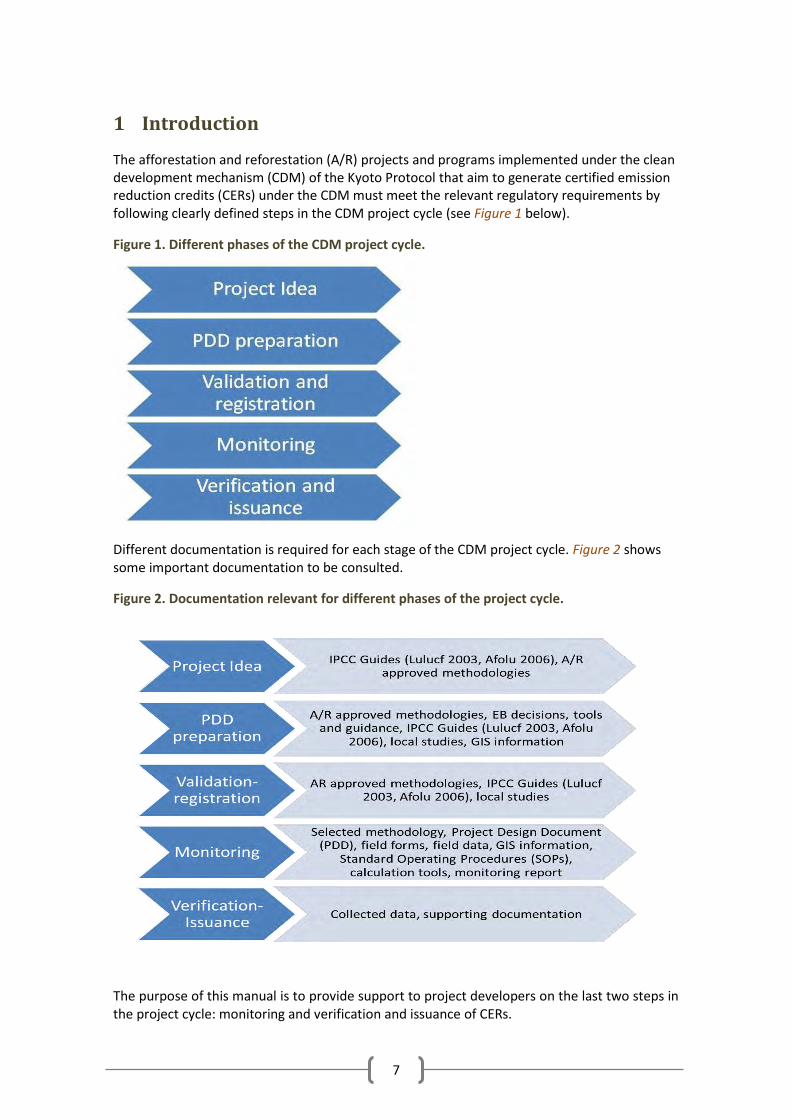
The afforestation and reforestation (A/R) projects and programs implemented under the clean development mechanism (CDM) of the Kyoto Protocol that aim to generate certified emission reduction credits (CERs) under the CDM must meet the relevant regulatory requirements by following clearly defined steps in the CDM project cycle (see Figure 1 below).

Figure 1. Different phases of the CDM project cycle.

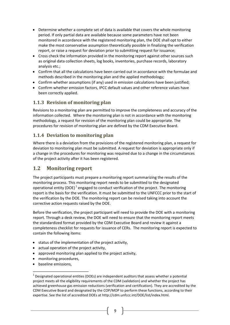
Different documentation is required for each stage of the CDM project cycle. Figure 2 shows some important documentation to be consulted.

Figure 2. Documentation relevant for different phases of the project cycle.

The purpose of this manual is to provide support to project developers on the last two steps in the project cycle: monitoring and verification and issuance of CERs.

8

1.1 Monitoring plan

Monitoring refers to the collection and archival of data and information relevant for a project. Monitoring is to be conducted following the monitoring plan adopted for the project. After the project is operational, project participants are required to implement the monitoring plan outlined as part of the project design document registered with the UNFCCC. Monitoring is a step necessary for verification, certification and issuance of credits. The monitoring plan of the PDD should identify methods of monitoring and measurement of carbon stocks of the project, data to be collected, growth parameters adopted along specific uncertainty levels, quality assurance and quality control procedures.

The monitoring of CDM A/R projects and programs requires organization of teams with knowledge of forest inventory, field data collection and quality assurance and quality control procedures relevant for the purpose. It also requires coordination of activities at the field level with clear definition of responsibilities of each member of the monitoring team.

The long term nature of forestry projects and the need for compliance of regulatory procedures require that data collected is accurate and it is stored in a secure format.

1.1.1 Compliance of monitoring plan and approved methodology

Although already addressed during the validation, the DOE is expected to again ensure that the monitoring plan in the PDD meets the requirements of the approved methodology applied by the proposed CDM project activity. If there are any issues, the DOE will need to request a revision to the monitoring plan before continuing and this will therefore delay the verification.

If the monitoring plan meets the requirements of the methodology, the second part of this step is to confirm that:

The monitoring plan and the applied methodology have been properly implemented and followed by the project participants;

All parameters stated in the monitoring plan, the applied methodology and relevant CDM Executive Board decisions have been sufficiently monitored and are updated as applicable, including: o Project emission parameters; o Baseline emission parameters; o Leakage parameters; o Management and operational system: the responsibilities and authorities for monitoring

and reporting are in accordance with the responsibilities and authorities stated in the monitoring plan.

The accuracy of the data collection and equipment used for monitoring meets the requirements of the monitoring plan (for example number of sample plots is sufficient to ensure required confidence interval). This also includes: o Ensuring that monitoring results are consistently recorded as per approved frequency; o Ensuring that quality assurance and quality control procedures have been applied in

accordance with the monitoring plan.

1.1.2 Ensuring the quality of data collected

The DOE will check the data and the calculations to ensure that the numbers reporting in the monitoring report are accurate. The DOE will:

9

Determine whether a complete set of data is available that covers the whole monitoring period. If only partial data are available because some parameters have not been monitored in accordance with the registered monitoring plan, the DOE shall opt to either make the most conservative assumption theoretically possible in finalizing the verification report, or raise a request for deviation prior to submitting request for issuance;

Cross check the information provided in the monitoring report against other sources such as original data collection sheets, log books, inventories, purchase records, laboratory analysis etc.;

Confirm that all the calculations have been carried out in accordance with the formulae and methods described in the monitoring plan and the applied methodology;

Confirm whether assumptions (if any) used in emission calculations have been justified;

Confirm whether emission factors, IPCC default values and other reference values have been correctly applied.

1.1.3 Revision of monitoring plan

Revisions to a monitoring plan are permitted to improve the completeness and accuracy of the information collected. Where the monitoring plan is not in accordance with the monitoring methodology, a request for revision of the monitoring plan could be appropriate. The procedures for revision of monitoring plan are defined by the CDM Executive Board.

1.1.4 Deviation to monitoring plan

Where there is a deviation from the provisions of the registered monitoring plan, a request for deviation to monitoring plan must be submitted. A request for deviation is appropriate only if a change in the procedures for monitoring was required due to a change in the circumstances of the project activity after it has been registered.

1.2 Monitoring report

The project participants must prepare a monitoring report summarizing the results of the monitoring process. This monitoring report needs to be submitted to the designated operational entity (DOE) 1 engaged to conduct verification of the project. The monitoring report is the basis for the verification. It must be submitted to the UNFCCC prior to the start of the verification by the DOE. The monitoring report can be revised taking into account the corrective action requests raised by the DOE.

Before the verification, the project participant will need to provide the DOE with a monitoring report. Through a desk review, the DOE will need to ensure that the monitoring report meets the standardized format provided by the CDM Executive Board and review it against a completeness checklist for requests for issuance of CERs. The monitoring report is expected to contain the following items:

status of the implementation of the project activity,

actual operation of the project activity,

approved monitoring plan applied to the project activity,

monitoring procedures,

baseline emissions,

1 Designated operational entities (DOEs) are independent auditors that assess whether a potential

project meets all the eligibility requirements of the CDM (validation) and whether the project has achieved greenhouse gas emission reductions (verification and certification). They are accredited by the CDM Executive Board and designated by the COP/MOP to perform these functions, according to their expertise. See the list of accredited DOEs at http://cdm.unfccc.int/DOE/list/index.html.

10

project emissions,

leakage emissions, and

emission reductions achieved during the monitoring period (including monitored parameters and calculation methods).

Please refer to part III of this manual for a more detailed description of the monitoring report template and requirements.

1.3 Verification

Verification is the independent review of the net anthropogenic greenhouse gas removals by sinks achieved, since the start of the project, by an afforestation or reforestation project activity under the CDM (5/CMP.1, Annex, paragraph 31) to be conducted by a Designated Operational Entity (DOE) based on the monitoring report submitted by the project participants.

The project participants can choose the time period of the first verification. The subsequent verifications and certifications shall be carried out at five year intervals until the end of the crediting period (5/CMP.1, Annex, paragraph 32).

The 41st meeting of CDM Executive Board decided to permit DOEs to request a change in the dates of a monitoring period undergoing verification, provided the change is the result of the corrective action request raised by the DOE during verification (EB 41, paragraph 78).

The verification will usually consist of a desk review and an On-site assessment. During the on-site assessment the DOE will:

Conduct a general assessment of the implementation and operation of the project;

Review the data collection and data handling process including a review of information flows for generating, aggregating and reporting the monitoring parameters. This will usually include interviews with relevant personnel to confirm that the operational and data collection procedures are implemented in accordance with the monitoring plan in the PDD. The DOE will likely want to see each step in the data collection and handling process to make sure that the chances of errors occurring are minimized in each step. Particular attention will therefore be paid to the quality control procedures and how these procedures are being implemented;

A cross-check between information provided in the monitoring report and data from other sources such as field records, inventories, purchase records or similar data sources;

The DOE will be looking for a clear audit trail that contains the evidence and records that validate or invalidate the stated figures. So if data are collected in the field on paper and put in a spreadsheet or database, the DOE will sample the original field papers to make sure they match the reported numbers. All this data and evidence will need to be made available to the DOE during the site-visit, if applicable collecting them in a central location. When reviewing the quality of the evidence, the DOE shall be assessing:

Whether sufficient evidence is available, both in terms of frequency (time period between evidence) and in covering the full monitoring period;

The source and nature of the evidence (external or internal, oral or documented, etc.);

If comparable information is available from sources other than that used in the monitoring report, then the DOE shall cross check the monitoring report against the other sources to confirm that the stated figures are correct.

11

1.3.1 Objectives of verification

Verification is the process of confirming the authenticity of greenhouse gas removals by an afforestation or reforestation CDM project over a defined monitoring period. The objectives of verification are to:

a) Ensure that the project activity has been implemented as per the registered PDD; b) Ensure that the monitoring report and other supporting documents are complete; c) Comply with the monitoring plan and the approved methodology; d) Assess the quality of data collected.

During the on-site visit, the DOE will assess that all physical features of the project as described in the registered PDD are in place and that the project is implemented as described in the registered PDD.

If the DOE thinks that the project activity does not conform to the description contained in the registered PDD, it must conduct an assessment on the potential impacts due to these changes. This assessment will mainly focus on:

Changes which may impact the additionality of the project activity. This might include issues such as use of different species or removal of one (or more) site of a project activity registered with multiple-sites;

Changes in the scale of CDM project activity. This is particularly important for small scale CDM projects;

Changes which impact the applicability/application of baseline methodology. This might include changes to the project that affect the applicability conditions of the methodology (for example if the applicability conditions of the methodology do not allow flooding irrigation and the project has decided to use this).

Section 2 introduces the Standard Operational Procedures presented in this manual to ensure compliance with regulatory requirements of A/R methodologies

2 Standard Operating Procedures

Standard Operational Procedures (SOPs) presented in this manual are a set of procedures to ensure successful monitoring of afforestation and reforestation projects and to facilitate acquisition of data as part of project monitoring. In the context, SOPs represent the established body of knowledge adopted for monitoring of projects to ensure compliance with regulatory requirements of A/R methodologies. A major purpose of the SOP use is to reduce or eliminate errors and uncertainties associated with monitoring and measurement of A/R projects.

In this manual, efforts have been made to ensure that the description of SOPs is comprehensive and rigorous, and that their implementation is likely to result in cost effective monitoring and measurement of GHG removals by sinks. The empirical field experience of implementing the A/R projects has been used in the development of the SOPs. Therefore, they are applicable to most project contexts.

However, modifications of SOPs may be required to deal with aspects specific to projects. The SOPs adopted for projects should continue to meet the compliance requirements of

12

methodologies while accommodating project specific circumstances. The cost of implementation, capacity requirements and field level constraints are taken into account in developing the SOPs.

The manual covers SOPs for the project activities covered in A/R methodologies, and that influence GHG removals by sinks of a project. The SOPs outline procedures; roles and responsibilities personnel associated with a project and guide the project personnel to implement relevant steps.

The purpose of this manual is to present hands on and actionable guidance on the implementation of SOPs. It does not seek to provide project specific instructions for use by the project personnel as each project has its own requirements and needs to implement monitoring systems that broadly conform to the SOPs.

Where possible, the information presented in this manual should be supplemented by the information from the good practices followed in the country and region of project location. In this context, personnel involved in project monitoring should review the requirements of the A/R methodology applicable to a project prior to adopting the relevant practices.

The SOPs outlined in this manual follow the requirements of afforestation and reforestation methodologies under the CDM. However, they can be applied for projects implemented under voluntary market regulation.

Revisions to the SOPs will be made based on the experience gained in implementation of A/R projects and revisions proposed to the monitoring plans of projects. Therefore, the project monitoring teams should consult the most recent version of this Manual.

The purpose, scope, prerequisites, responsibilities of personnel involved in monitoring and quality assurance and quality control provisions of SOPs are described in the following sections of the manual.

Sections 3 to 8 present the main monitoring elements required for the monitoring of a CDM A/R project activity.

3 Monitoring project boundary

CDM A/R activities are usually implemented in more than one land parcel. Each individual land parcel is called a discrete area with unique geographical identification and boundary. The Project boundary is defined by aggregating the boundaries of all the discrete areas that are part of a project.

Within a project, the discrete areas are grouped into strata. The purpose of dividing a project area into strata is to group the discrete areas with similar forest growth features so as to lower the cost of monitoring without reducing measurement precision (see Section 6.1.1 - Stratification for details). A stratum is refers to group of discrete areas that conform to one or more stratification factors (such as species, soil type, management) that influence the carbon stocks of the stratum. Depending on project design, a discrete area might be part of one stratum or multiple strata might occur on a discrete area.

All A/R methodologies require that boundaries of a project are clearly defined at the start of the project. Most approved CDM A/R methodologies additionally require that the area of each stratum and of the project as a whole are monitored during the crediting period, either by field measurements using GPS, official forest management maps or remote sensing techniques

13

(such as aerial photographs). Monitored areas must be checked for consistency against the boundaries reported in registered PDD. If field measurements are collected using GPS, it is good practice to follow the relevant Standard Operating Procedure (SOP) for collection of project boundary data. Projects can utilize the SOP 1- Collection and organization of data using GPS, or develop their own SOP. SOP 1 can also be used for locating permanent sampling plots and for monitoring of forest disturbances.

SOP 1 - Collection and organization of data using GPS

Standard Operating Procedure for collection and organization of data using GPS

Purpose

The purpose of collecting GPS data on project activities such as demarcating project boundary, identification of strata and laying out sample plots in an A/R project or program is intended to facilitate monitoring of all activities that require geographic identification.

Scope

This SOP requires a basic knowledge of GPS operation and ability of field personnel to record points and waypoints on in the field and to download the recorded data to a computer. The Global Positioning System (GPS) is a space-based satellite navigation system that provides reliable information on the location of geographic units by measuring distance from a group of satellites in the space. References on the use of GPS can be accessed over the Internet. Please visit http://www.cmtinc.com/gpsbook/ for a text introduction; and http://www.trimble.com/gps/index.shtml for visual demonstration on the use of the GPS.

Prerequisites for the use of GPS

GPS receiver

Maps (mostly exist in the GPS)

Field notebook and pen

Computer (for data processing).

Data transfer cable

GPS mapping software

Internet access

Basic knowledge of GPS use

Responsibilities

Person in charge of GPS receiver: check that GPS receiver has enough charge/ batteries for planned field work, set appropriate coordinate system and configure the GPS prior to taking readings in the field. Record GPS filenames and datum on datasheets. Follow the quality assurance/quality control procedures applicable to the respective field personnel. Field crew supervisor: check the quality of collected data and verify a subsample of collected

data. GIS manager or assistant: should receive and process GPS files, store field data and check for

the consistency of collected data with existing databases/map layers.

14

Procedure for monitoring boundaries (of discrete areas or disturbed areas)

Turn on the GPS unit and allow it to initialize to gather location information and to identify GPS satellites. This process can take several minutes. The GPS unit's main screen will display when it is complete.

Note the dilution of precision (DOP) error. The DOP measures the error caused by the geometry between the user and the satellites. This information will indicate map accuracy. The GPS user manual may be referred for information on how to find the DOP.

Begin by setting a waypoint at starting location. A waypoint records the GPS coordinates of a user-defined location. Some GPS units will have a button on the outside of the unit. Others may require navigating to a menu. The GPS user’s manual may be referred for instructions.

Decide whether you want to plot a map with a track or a route. With a track, the GPS unit automatically records GPS coordinates along your direction of travel at a predefined distance. A route shows a path of waypoints that you collect as you move. If you are unable to travel the distance of the area you want to map because of topography or terrain (e.g., wetland in the way), a route is the better option.

Follow the perimeter of the area you wish to plot. Note distinct features for setting a waypoint. Most GPS units allow you to include description, but typing text in the GPS is a slow process. Therefore, carrying a field notebook to note the names and descriptions of the points of traverse is recommended.

After moving along the track boundaries, return to the beginning waypoint. If you set up a tracking feature, stop the tracking through GPS unit's menu.

Upload the GPS coordinate data to the computer and process it with mapping software. The user manual of the mapping software may be consulted for instructions. Most mapping software programs permit inclusion of information recorded in the field notebook while traversing along routes and/or waypoints.

Procedure for locating permanent plots

Turn on the GPS unit and allow it to initialize for gathering location information and for identifying the satellites. This process can take several minutes. The GPS unit's main screen will display when the process is complete.

Note the dilution of precision (DOP) error. The DOP measures the error caused by the geometry between the user and the satellites. This information indicates the accuracy of reading. Refer to the GPS manual for information on how to find the DOP.

For rectangular or square plots, set waypoints of all plot corners. A waypoint records the GPS coordinates of a user-defined location. Some GPS units will have a button on the outside of the unit. Others may require navigating to a menu. The GPS user’s manual may be referred for instructions.

In the case of circular plots, set a waypoint at the center of plot.

Upload the data on GPS coordinates to the computer. Some GPS units, such as Garmin or Trimble devices, have proprietary mapping software that can be purchased along with the unit. The software programs allow inclusion of information recorded in the field notebook while traversing along routes and/or waypoints.

Quality assurance and quality control

Data collection

Regardless of the type of GPS receiver, data collection standards and quality control measures

15

shall be followed in order to produce accurate data.

Satellite availability: GPS device must track at least four satellites to get a 3-D position.

Satellite geometry or distribution of satellites in the sky affects the computation of your position. This is often referred to as Position Dilution of Precision (PDOP). Satellites that are spread out have better geometry and give accurate reading than when they are clustered together. PDOP is determined by geographic location, the time of a day on which measurements are made, and obstructions that block satellite signals. PDOP is expressed as a number. The lower PDOP numbers are preferable to higher numbers. On some GPS receivers. PDOP can be adjusted to allow for recording of points at different levels of accuracy. The best results are obtained when PDOP is less than 7 (PDOP of 6 is preferred). The user should not increase the allowable PDOP value to more than 8 unless data on a position is collected overriding the accuracy. In the flexible field work schedules, GPS users should increase mapping accuracy by using planning charts and targeting the data collection during the times of a day when satellite availability and geometry are best.

Length of time GPS data file is open: Positional accuracy will be better the longer a file is open and more GPS positions are collected and averaged. The GPS user manual may be consulted for relevant guidance).

Multi-path error or signal interference: Multi-path error occurs due to the reflection of signals. GPS signals may be reflected by surfaces near the antennae, causing error in the travel time and the GPS positions. Although the multi-path error is mostly beyond the control of a GPS user, adjustments such as positioning the GPS with unobstructed view of the sky, using offsets from better satellite reception areas to the target location (refer to 0 below), and using an external antenna could minimize the likelihood of this error.

Data handling

Personnel involved in the monitoring are trained to verify the geographic boundary and to record the data in the project database for reporting at the time of project verification.

The monitored data and information on the boundary are checked to ensure consistency with the data recorded in the project database and the registered PDD; and reasons, if any, for the change are recorded.

Monitoring procedures of the project boundary need to ensure that the land use activities within and outside of the project can be identified.

It is important that field crews returning from the field should transfer GPS files to the database and backed-up storage. Files should be transferred to an appropriately-named folder (such as “Raw” or “Backup”). Communicate with the GPS support person to determine how the files are stored as well as differentially corrected (if required2), and entered into the database.

2 Differential correction techniques are used to enhance the quality of location data gathered using GPS

receivers. Differential correction can be applied in real-time directly in the field or when post processing data in the office.

16

SOP 2 - Using offsets during GPS data collection to improve satellite reception

Standard Operating Procedure for using offsets during GPS data collection to improve satellite reception

Purpose

The purpose of this SOP is to describe the use offsets during GPS data collection in case of signal interference and difficulties in getting a reading of sufficient quality (preferably based on four satellite signals with PDOP < 8.0).

Scope

This procedure is intended for field crew and field crew supervisors in monitoring of project boundary, monitoring of strata and laying out permanent sample plots, when the GPS receiver cannot read a specific location because of signal interference.

Prerequisites

GPS receiver

compass

measuring tape .

clinometer (optional)

Procedure

Move from the location of interest to the nearest location at which you can obtain satellite coverage of GPS position as indicated in Figure 3.

Figure 3. Offsetting points of interest using GPS receiver.

Temporarily mark this location (you will later need to measure distance and azimuth from here to the target, and enter this into the GPS unit and onto the data sheet).

Open a GPS file and record the file name and your current location as described above.

17

Move to Plot Center (c) with your compass and measuring tape. First move from a to b; then move from b to c. Be sure to use horizontal distance. You may account for slope by keeping the measuring tape level (as shown in Figure 4), using a laser range finder to measure distance, or measuring the slope with a clinometer and using a slope corrections table to calculate horizontal distance from slope distance.

Figure 4. Measuring distances in slopes.

Calculate the distance and azimuth from the GPS location to the newly determined plot center. Record this offset distance and azimuth on the data sheet.

Record this offset in the GPS. Make sure that you enter the distance and azimuth from the GPS location to the newly determined plot center (a to c). Offsets entered into the GPS unit file are preferable because the software will incorporate it during post-processing.

Quality assurance and quality control

See SOP 1- Collection and organization of data using GPS for QA/QC procedures.

4 Species data

Basic information of species to be used in the implementation of an AR CDM activity must be collected in order to calculate the carbon stock changes based on sample plots of a project or program.

Data on species growth affects the number of emissions reduction credits that may be obtained from a CDM A/R project, e.g., an increase in wood density from 0.35 to 0.45 may positively influence the number of emission reduction credits and vice versa. Therefore, choice of appropriate growth data is a key to accurate calculation of the emission reductions.

4.1 Collection of species data

The Standard Operational Procedure for collecting species data are outlined below.

Section 10.2 presents websites relevant for collecting species data.

18

SOP 3 - Collection of species data

Standard Operating Procedure for Collecting Species Data

Purpose

To outline the steps to be followed in collecting data on species growth and characteristics required for calculation of carbon stock changes.

Scope

This procedure is intended for the personnel in charge of defining parameters for calculation of carbon stock changes of an A/R project or program.

Prerequisites

Registered PDD or PoA-DD and CPA-DD

Requirements

Registered PDD

Procedure

In order to collect data and information on parameters of species growth, the following procedure should be followed.

List of species or groups of species

Collect information on stand models and species composition (monoculture, mix of species) and method of regeneration from the registered PDD.

Compare the species information presented in the PDD with the information available at implementation. If there are deviations from the PDD in terms of the species and stand models implemented, such deviations should be described and justified in the monitoring report. Prior to verification, the list of species included in the project should be compared with those listed in the PDD, and previous monitoring and verification reports (if any).

Based on the review of PDD, assess if biomass growth of species can be calculated separately or in groups of species. Depending on the stand models used, data and information available on individual species, and growth characteristics of species, their grouping may be required. A species group may be defined for species that grow together in a stand, or if they have similar growth characteristics (e.g. species belonging to a genus are likely to have similar growth characteristics). Some projects may plant small areas of many native, less known species, either in pure or in mixed stands, grouping is acceptable in situations of sparse data where each individual species forms a small proportion of a stand or a stratum.

For each species or species group, the following data and information need to be collected:

o name of species (Latin and common name in the region), o species with similar growth characteristics, o method of calculation of above ground biomass: (i)biomass expansion factor

(BEF) method or (ii) allometric method o For project using the BEF method:

Approach for estimating total or merchantable stem volume in m3 from dbh and/or height (for example volume equation or volume

19

table) biomass expansion factor (BEF method),

o For projects using the allometric method: allometric equation specifying relationship, between tree above

ground biomass in tons of dry matter and diameter at breast height and/or tree height and the

o root shoot ratio, o wood density, o carbon fraction and

If BEF method is used for calculation of carbon stock change in the project, then appropriate biomass expansion factor should be adopted. If allometric method is used for calculation of carbon stock change, then the relevant allometric equation(s) should be defined. The following sources of data may be used, in order of preference:

Data included in the registered PDD

Local published studies or unpublished studies with supporting documentation pertaining to species growth parameters.

Published studies and data at country or regional level (see Section 10.2 –References and useful websites).

Default values from IPCC (see IPCC - 2003 - GPG for LULUCF Tables.xls and IPCC - AFOLU guidelines 2006 tables.xls)

Quality assurance and quality control

The monitoring team should periodically check the validity of parameters and equations used for calculations, preferably with growth data of species applicable to the project area.

4.2 Updating species data

Some parameters and equations are not constant during the lifespan of the project and may vary to a great extent (e.g., biomass expansion factors are age-dependent and tend to decrease with age, while average wood density should increase as trees age) and should be updated to increase the accuracy of calculations.

SOP 4 - Laboratory wood density determination

Standard Operating Procedure for laboratory wood density determination

Purpose

Describe the process of determining wood density using maximum moisture content method3.

Scope

This procedure is intended for laboratory workers or monitoring staff determining wood density.

3 Smith, Diana 1954. Maximum moisture content method for determining specific gravity of small

wood samples. Forest Products Laboratory, Forest Service, U.S. Department of Agriculture. 9 pp.

20

Equipment

Laboratory oven

Electronic weighting scale with a minimum precision of 0.01 gr.

Prerequisites

None.

Procedure

Figure 5. Equipment for determination of wood density.

Submerge wood samples in water until saturation is reached and weigh saturated samples. Then, dry samples at 105°C for 26 hours. Extract samples from oven and weigh them again. Do this last weight quickly, withdrawing samples from oven immediately before weighing them, so that no moisture is absorbed by dried samples before obtaining weights.

Wood density is calculated as

1

1

1.53

Dmps po

po

Where: Dm = Wood density Ps= Saturated weight of sample (g) Po= Anhydrous weight of sample (g) 1.53 = Wood density constant.

Quality assurance and quality control

A person different to the one in charge of determining wood density should select randomly 5% of the samples and repeat the procedure. The re-measurement data may be compared with the original measurement data. Errors assessed in the prior measurements need to be corrected, recorded and used to calculate the measurement error.

5 Monitoring project implementation

The activities of project implementation and events that could impact the expected amount of removals need to be monitored as per the requirements of A/R methodology applicable to project and monitoring procedures outlined in the PDD. The monitoring requirements of large scale and small scale methodologies may be different. Therefore, monitoring steps and guidance outlined in the respective A/R methodologies need to be followed consistently.

The project implementation consists of site preparation and forest establishment. Standard Operational Procedures for activities associated with them are presented in the next sections.

21

5.1 Site preparation

Site preparation includes activities undertaken for preparation of the sites for planting such as removal of preexisting vegetation (including biomass burning, if permitted in the applicable CDM A/R methodology) and soil preparation. Monitoring of biomass burning is addressed in SOP 20.

SOP 5 - Monitoring site preparation

Standard Operating Procedure for monitoring site preparation

Purpose

To describe the process of collecting data for monitoring of site preparation.

Scope

Monitoring of site preparation is required by large scale CDM A/R methodologies. However, small scale CDM A/R methodologies do not anticipate monitoring of site preparation. Therefore, monitoring of site preparation is mostly relevant for persons with supervisory responsibilities that oversee site preparation activities of large scale A/R projects.

Prerequisites

Monitoring of project boundaries.

Requirements

GPS

Field forms

Registered PDD

Procedure

Site preparation depends to a large extent on local characteristics, pre-existing vegetation, use of machinery and equipment, species proposed in a project and method(s) of planting, etc., and thus, monitoring parameters and procedures of monitoring should be adopted as per the guidelines of the methodology applied and characteristics of a project.

Monitoring of site preparation activities is initiated prior to starting field operations of an A/R project. The PDD should be checked to identify the site preparation activities that are in line with those proposed in the PDD.

It is important to check that the biomass burning is not used for site preparation unless allowed by the approved methodology.

If planting is accomplished over several years, activities of each planting year need to be monitored.

For each site preparation activity, the relevant data needs to be recorded, e.g.,: o Date, location and area affected in site preparation. If affected area is different

from that defined in the PDD (e.g. partial site preparation of a given discrete area), then area affected by site preparation should be measured and reported. If GPS is used to determine the area of site preparation activity, SOP 1and 0 may be referred.

o Type of site preparation activity (e.g. digging of pits, pre-existing biomass removal) including site clearance and cleaning activities, if any undertaken.

o Information on the whether or not biomass is burned as part of the site preparation needs to specified. If biomass is burned, then SOP 20 may be

22

referred. o Equipment and machinery, if any, used in the site preparation. o The size of pits dug and spacing followed in digging of pits for the purpose of

planting.

Quality assurance and quality control

Personnel different from those in charge of filling site preparation reports must check and conform within a month of site preparation activities implemented to ensure that:

Site preparation activities implemented on each discrete area are reported.

The summation of area of site preparation must equal the total area of site preparation reported during planting period.

Forms are correctly filled and there is no missing information. Project and discrete areas ID codes are consistently used.

Reported activities are in compliance of methodology steps and procedures outlined in PDD.

A predefined percentage of the discrete areas (e.g. 5 or 10%, depending on the differences among strata) should be checked in the field soon after the site preparation is completed in order to check the quality of the accomplished activities and ensure conformity with procedures outlined in the PDD and/or practices common to the region.

5.2 Forest establishment

Forest may be established by seeding and/or planting of seedlings and/or or through assisted natural regeneration. For several methodologies, forest establishment must be recorded as part of the monitoring process.

SOP 6 - Monitoring forest establishment

Standard Operating Procedure for monitoring forest establishment

Purpose

To describe the process of collecting data for monitoring of forest establishment.

Scope

This procedure is intended for supervisors and equivalents that oversee activities for forest establishment.

Prerequisites

Monitoring field form/datasheet on project boundaries

Monitoring field form/datasheet on site preparation

Requirements

GPS

Field forms

Registered PDD

Procedure

The monitoring of forest establishment includes follow up of the post-planting activities that

23

influence forest establishment. These activities implemented subsequent to seeding, planting or those implemented to promote natural regeneration are monitored. If forest establishment activities are performed in several years, each activity season must be monitored. The monitoring of forest establishment includes:

Data pertaining to species composition, spacing, and planting schedule are monitored.

Information on planting stock, method of planting and technologies used are assessed.

The occurrence of droughts and floods and other emergencies that influence the forest establishment is monitored.

Deviations from the planned activities are assessed to examine their influence on the project activities.

Areas with the survival rate lower than the established indicators are replanted. The area and location of supplemental plantings undertaken to fill the gaps are recorded in the project database.

Quality assurance and quality control

Personnel different from supervisors or personnel in-charge of filling the forest establishment forms must check the activities within one month after the end of the planting season and should verify that:

Each discrete area proposed for seeding/planting/assisted natural regeneration implemented the relevant activities.

Planted species and planting densities conform to the details presented in the PDD. Any deviation must be explained and justified.

The summation of discrete areas reported as planted equals the total to the area proposed for planting. Any deviation must be explained and justified.

Forms are correctly filled without missing information. Project and discrete area ID codes are consistently used.

A pre-defined percentage of the discrete areas (e.g. 5 or 10%, depending on the differences among strata) should be visited in the field after planting activities are completed in order to check the quality of activities implemented and their conformity with the procedures outlined in the PDD and/or practices common to the region.

5.3 Survival plots

Survival rates of all planted areas of the project must be assessed and recorded as part of project monitoring. Survival rates are assessed using survival sampling plots. These plots may be the same that will be used for assessing carbon stocks or they may be temporary plots.

Surveys using sample plots are conducted to evaluate the survival rate of planted seedlings. The procedure for establishing plots is described in Section 6.2.1 - Establishment of permanent trees sample plots. The procedure for calculating survival rate is explained in SOP 7- Monitoring survival of planted trees. The use of permanent sample plots for assessing trees survival is not mandatory and temporary plots may be used. If temporary plots are used, a different sampling design may be used, e.g. by using different plot size and form (circular plots may be more efficient for counting surviving trees), or counting live trees along existing plantation rows of fixed length.

24

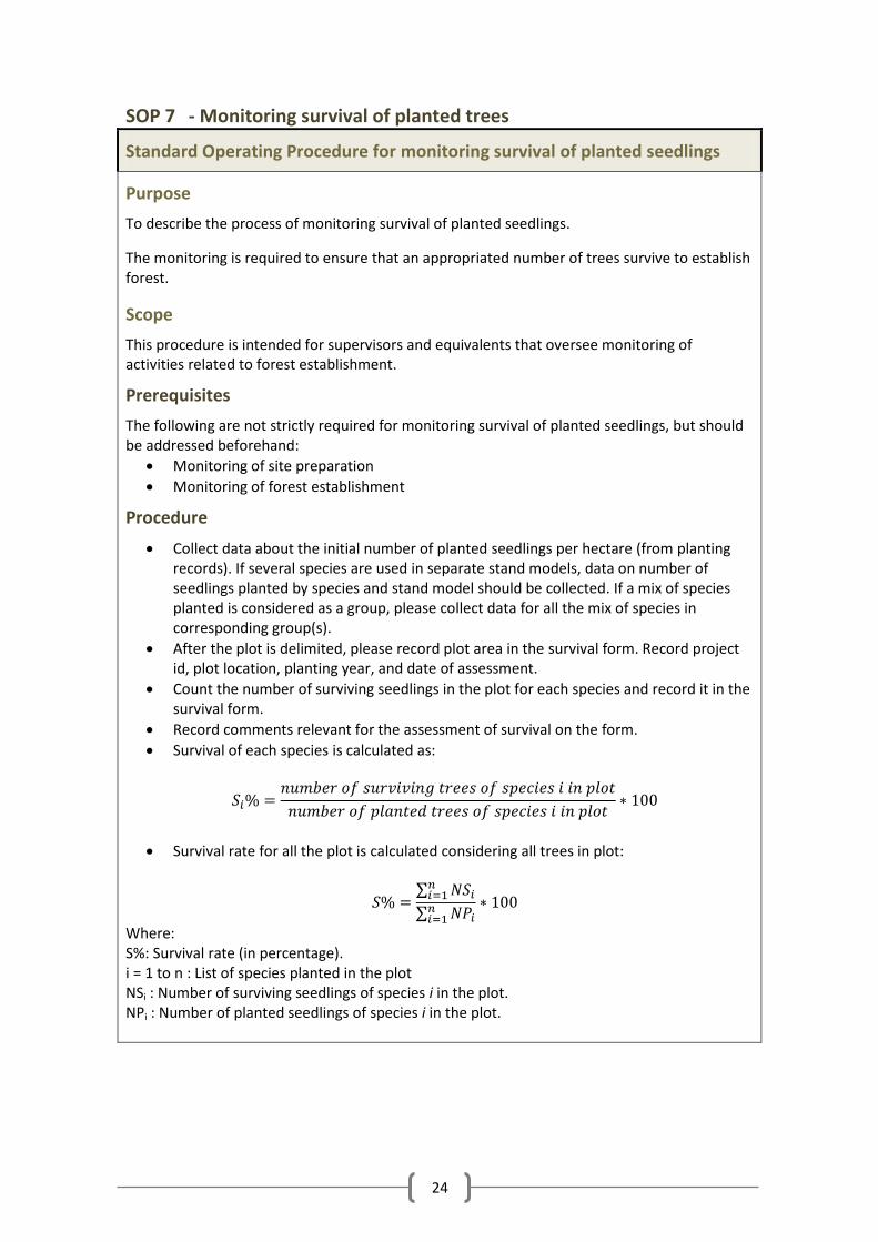
SOP 7 - Monitoring survival of planted trees

Standard Operating Procedure for monitoring survival of planted seedlings

Purpose

To describe the process of monitoring survival of planted seedlings.

The monitoring is required to ensure that an appropriated number of trees survive to establish forest.

Scope

This procedure is intended for supervisors and equivalents that oversee monitoring of activities related to forest establishment.

Prerequisites

The following are not strictly required for monitoring survival of planted seedlings, but should be addressed beforehand:

Monitoring of site preparation

Monitoring of forest establishment

Procedure

Collect data about the initial number of planted seedlings per hectare (from planting records). If several species are used in separate stand models, data on number of seedlings planted by species and stand model should be collected. If a mix of species planted is considered as a group, please collect data for all the mix of species in corresponding group(s).

After the plot is delimited, please record plot area in the survival form. Record project id, plot location, planting year, and date of assessment.

Count the number of surviving seedlings in the plot for each species and record it in the survival form.

Record comments relevant for the assessment of survival on the form.

Survival of each species is calculated as:

Survival rate for all the plot is calculated considering all trees in plot:

∑

∑

Where: S%: Survival rate (in percentage). i = 1 to n : List of species planted in the plot NSi : Number of surviving seedlings of species i in the plot. NPi : Number of planted seedlings of species i in the plot.

25

Quality assurance and quality control

Personnel different from the staff in charge of establishing and monitoring survival in the plots, must check the survival data within a month of the collection of survival data to ensure that:

Each stratum is considered in the report.

Discrete areas are appropriately represented in the survival sampling (see Section SOP 8 Stratification).

Survival check forms are correctly filled with no missing information.

Project and discrete areas ID codes are consistently used on the survival check forms. A pre-defined percentage of the survival sampling plots (e.g. 5 or 10%) should be visited in the field soon after activities are finished to check the quality of the accomplished activities. If survival rates of the re-sampled plots differ by more than 10% to the original sample, then a full re-assessment of survival plots need to be conducted.

5.4 Silvicultural activities

Silvicultural activities include fertilization, pruning, thinning, harvesting, coppicing and other operations that influence the GHG removals. Monitoring of silvicultural activities can involve a large number of parameters such as quantity of fuel wood collected or timber harvested, checking lands that are re-planted or re-sown after harvesting, checking for natural regeneration in harvested land, monitoring of disturbances such as fires, floods and windfall etc. The list of activities to be considered may vary according to the characteristics of each project, even if projects follow the same methodology.

The procedure for monitoring of silvicultural activities consists of tracking dates and areas affected, and preparation of report with a summary of activities implemented (e.g., stand or discrete area ID, type of activity, area affected and other relevant data No GHGs emissions reporting are required for silvicultural activities as these are reported separately under project emissions (See Section 7. Monitoring project emissions). Depending on the methodology, activities identified as sources of GHG emissions may include: Biomass burning (if done as part of silvicultural operations), use of fossil fuels (for transportation; and operation of machinery such as chain saws etc.) fertilization and fencing with wood from non-renewable sources.

The monitoring of each silvicultural activity should include information on discrete area, name of activity, date(s), location, area, species, volume or biomass affected etc.

5.5 Disturbances

Information on the type of natural disturbances (e.g., fires, floods, landslides, pest outbreaks etc.) or human induced disturbances (e.g., illegal felling, intentional fires) should be monitored and recorded. Monitoring of disturbances may include date, location, area affected (as per the GPS coordinates or field survey), tree species, biomass lost, corrective measures implemented, and change in the boundary of strata or stands due to the disturbance.

As part of ex post stratification, the boundaries of project strata may need to be revised taking into account the disturbances affecting the discrete area of the project.

Some methodologies require the monitoring of disturbance, while others do not require the monitoring of disturbances if the effects of disturbance are captured through the monitoring

26

of permanent sample plots. Therefore, the requirements of applicable methodology with regard to the monitoring of disturbance should be followed.

6 Monitoring carbon stocks

Carbon in forest ecosystems is stored in different pools or reservoirs. They are grouped into five major pools (see Figure 6). The aboveground and belowground biomass are part of the standing tree vegetation, but are considered as separate pools because of the differences in procedures of estimation of the two pools.

Figure 6. Carbon pools in a forestry project and corresponding methods for their estimation.

6.1 Sampling framework

The carbon stocks of forest can be estimated based on the measurement of growth of tree and non-vegetation on permanent sample plots. The sampling framework describes the procedures for stratification of a project, calculation of the number of sample plots required for monitoring and their location and layout in the project area.

6.1.1 Stratification

The discrete areas of a project are heterogeneous in terms of site conditions, vegetation cover and soil type. Stratification of the project area into relatively homogeneous units can either increase the precision of carbon stock change estimates without increasing the cost unduly, or reduce the cost without decreasing precision of carbon stock estimates by lowering variance of carbon stock change estimates.

Stratification is accomplished ex-ante for both the baseline scenario (usually based on previous land use or land cover) and for the project scenario. Stratification of the project scenario is done taking into account the site characteristics, species planted (or groups of them if several tree species have similar growth habits or are planted in mixed stands) and grouped into age classes or other specific criteria depending on the characteristics of a specific project.

The need for ex post stratification may arise due to changes to a project from a variety of factors such as:

Deviation from the planting schedule proposed at the time of project design

Differences in growth rates of species in project strata

Disturbances affecting carbon stocks of part(s) of strata

27

When stratifying a project, the differences among strata should be easily identifiable; i.e., strata boundaries should be defined based on prominent features such as species, slope, planting year etc. Otherwise, the difficulties in locating strata and likelihood of errors in their identification on the ground outweigh the benefits of defining them.

As a rule of thumb, the area of a given stratum should not be less than 10% of the total area to be sampled (which implies that no more than ten strata should be defined). Another approach to restrict the total number of strata is to consider areas pertaining to different strata if they have a difference of 10% or more of mean carbon stocks. I.e., if an area has an average of 200 t-C/ha and another one has 182 t-C/ha, these could be considered as a single stratum, since the difference in carbon stocks is less than 10%.

If the number of strata is changed, project should remember that most methodologies calculate carbon stock changes between two points in time (t1 and t2) at the stratum level, and then all strata are summed to obtain total carbon stock difference. If new strata are created from the existing strata, the areas of respective strata/substrata also need to be revised (see Figure 7).

Figure 7. Stock change method for subdivided strata.

6.1.2 Revision to project strata

Stratification may need to be revised as prior stratification may not adequately represent the status, growth and characteristics of a project. For example, if fire burns a part of a stratum, burnt areas should be considered as a separate stratum or combined with similar areas of another stratum.

Prior to starting monitoring of carbon stocks during each verification period, the project monitoring team should review the stratification in order to ensure that:

28

Existing stratification as outlined in the PDD is efficient and to determine if the strata are adequate and if grouping some of the strata or their division into additional strata is appropriate.

Stratification factors (e.g. species, year of planting, growth rate, etc.) continue to be relevant during the project period. It needs to be assessed if new factors or factors not previously considered affect the carbon stocks of project. The potential stratification factors should not affect a whole stratum, but part of one or more of strata. If a potential new factor affects a whole stratum, then it is of no use for stratification, since it will be of no help in subdividing into homogeneous areas.

Stratification levels (e.g. list of species, planting years, etc.) need to be assessed for their adequacy in reflecting the significant differences in carbon stocks, e.g., if planting year is a stratification factor, and each planting year is considered a level; and If it is found that a difference of one year in age does not result in significant differences in carbon stocks, the stands of a species with age classes of two or more years could be considered as part of the same stratum.

The re-stratification may result in few or more strata in comparison to the strata defined at the starting of the project. However, the number of strata adopted should adequately capture the variance in carbon stock change. It is good practice to have no more than 10 or 12 strata and to avoid defining strata with very small areas.

The purpose of stratification should be to partition natural variation of project biomass and to reduce monitoring costs. If stratification leads to no change in costs or minimal change in costs, then it may be of limited value.

Re-stratification will require revision to the calculation of required number of sampling plots. The existing sample plots are to be preserved in the respective strata and are assigned to new strata as per the re-stratification. If the number of existing plots in a redefined stratum is smaller than the number of required plots, then new plots must be located for completing the sampling framework. Plots should be located in project strata (i.e. randomly or systematically) according to the methodology.

In the case of new strata, the required number of plots should be calculated and located using standard operating procedures (See SOP 9 - Determining sample size and SOP 10- Random location of sample plots or SOP 11- Systematic location of sample plots).

SOP 8 – Stratification/Re-stratification

Standard Operating Procedure for stratifying the project area

Purpose

To describe the process of stratifying the project area.

Stratification is the grouping of the area of a project into homogeneous units in terms of carbon stocks, using stratification factors (such as species, soil type, management) that could affect carbon stock.

Scope

Stratification facilitates assessment of sample size required to reach a given level of precision in estimation of carbon stock change during the monitoring period.

29

Prerequisites

Monitoring of project boundaries

Monitoring of project implementation Maps of a project area and information on factors that affect carbon stocks are required for the purpose of stratification or its revisions.

Procedure

Step 1: The key factors influencing carbon stocks in the above- and below-biomass pools need to be assessed. These may include soil characteristics, landform (e.g., elevation, slope gradient), tree species to be planted, years of planting, management, etc. Step 2: Collection of information on key factors identified in step 1, e.g.: • Data and maps of project sites reflecting the factors; • Land use/cover maps and/or satellite images / aerial photography; • Soil and cadastral maps showing physiographic features, geology, soil characteristics, erosion

status etc.; • Other data and information pertaining to stratification factors available from records, study

reports and publications of national, regional or local governments or institutions, and literature.

The following factors shall be considered in the ex-post-stratification: • Data from monitoring of forest establishment and project boundary, e.g., actual project

boundary, site and soil preparation, tree species and planting year; • Data from monitoring of forest management, e.g., pruning, thinning, harvesting are taken

into account to assess the changes in carbon stock changes for each stratum and substratum during monitoring period.

Previous results from measurements in permanent sample plots or from measurements for silvicultural management of plantations.

Step 3: Preliminary stratification/stratification shall be conducted in a hierarchical order taking into account the key factors influencing carbon stock or the extent the key factors differ across the project area (e.g. rainfall). At each level in the hierarchy, stratification shall be conducted within the strata determined at the upper level. For example, if there is a significant climatic difference within the project boundary, the stratification process may begin with stratification according to difference of the climate. If the key factor in the second level is soil type, then strata determined in the first level may be further stratified based on difference of soil type. Stratification could also be carried out on GIS platform by overlaying maps/information collected. Step 4: Supplementary survey of sites of preliminary stratum, e.g.: • Tree vegetation: species, age class, number of trees, mean diameter at breast height (DBH)

and/or height of trees on randomly selected plots (at least three plots for each stratum); • Non-tree vegetation: crown cover and mean height of shrubs of sub-plots in the plots for

measuring trees; • Site and soil factors: soil type, soil depth, slope, erosion, underground water level, etc.; • Human impacts: biomass burning, logging, grazing, fuel collection etc.; If the variation is large within each stratum, further field investigation shall be conducted and/or further stratification shall be considered in step 5.

30

Step 5: Conducting a further stratification based on supplementary information collected from step 4 above, by checking whether or not each stratum is sufficiently homogenous or the difference among strata is significant. A stratum that shows significant variation in its vegetation, soils and human intervention shall be divided into two or more strata. On the other hand, strata with similar features shall be merged into one stratum. Distinct strata should differ significantly from each other. For example, sites with different species and age classes of trees shall form a separate stratum. Sites with a more intensive grazing or fuelwood collection might also be treated as separate strata. Step 6: Sub-stratification: Create sub-strata for each stratum based on tree species and/or on planting year. Step 7: Create stratification map, preferably using a Geographical Information System (GIS). The GIS will be useful for integrating data from different sources and to stratify the project area. Ex post stratification shall be considered to take into account the changes in project boundaries, species planted, stand models adopted, and year of planting in comparison to the information presented in PDD.

Quality assurance and quality control

A person who was not part of team associated with stratification should review the procedures and check:

That the proposed stratification complies with the registered PDD. Any deviations from the PDD should be justified.

Area of strata and total project area are cross checked.

Checks need to be performed to ensure that all discrete areas are included in stratification.

It should be insured that data and information stratification factors or criteria is verifiable.

6.1.3 Stratification example

Figure 8. Stratification example.

The boundary of CDM AR project under implementation.

The two species are selected for planting on two soil types of the project.

31

The stands of two species are planted in different years on two soil types. For this example, stands are named with letters, from A to I.

Stands sharing the same characteristics (or having same stratification factors) are considered part of the same stratum.

Once stands or discrete areas are grouped into strata, boundaries of stratification factors are not anymore required.

Sample plots established following a sample frame in a stand or discrete area are statistically representative of the rest of stands or discrete areas representing the same stratum; hence, sample plots located in stands or discrete areas adequately represent the changes in the carbon stocks of a project.

6.1.4 Determining sample size (number of sample plots)

Projects must calculate the number of sample plots needed for monitoring and measurement in order to meet the targeted precision level4 of carbon stock estimation required by the methodology. The project contains heterogeneous areas in terms of trees species, years of planting, growth rates, soil characteristics and climatic conditions, which contribute to variability in the carbon stock estimates5. The variability in the project can further increase due to:

4 Technically defined, precision level is a measure of the spread of a confidence interval. The narrower

the interval, the higher the level of precision. In a general sense, precision is how well a value is defined. In sampling, precision illustrates the level of agreement among repeated measurements of the same quantity. Precision is the inverse of uncertainty in the sense that the more precise something is, the less uncertain it is. Precision level is measured in percentage and is often used for meaning “Error level”. Some methodologies and PDDs state a target precision level of 10%, willing to mean an error level of 10% . 5 Variability in carbon stocks can be dimensioned by calculating standard deviation, a measure of the

spread of the data.

32

Variability in the growth rates of species in response to forest management activities and disturbances.

Unexpected disturbances occurring during the crediting period (e.g. due to fire, pests or disease outbreaks), affecting various parts of an originally homogeneous areas;

Forest management activities (cleaning, planting, thinning, harvesting, coppicing, replanting) that are implemented could affect the project area differently; and

The higher the variability in carbon stocks of a project, the more sample plots are needed to meet the targeted precision. By grouping the project area into relatively homogenous strata, the stratification is expected to lower the number of sample plots required for assessment of carbon stock changes during the monitoring period.

During the life time of the project, the project needs to ensure that the number of sample plots continue to meet the targeted precision level. Therefore, if variability in carbon stocks of increases due to species, soil or disturbance related factors, a project can select to revise the number of strata and/or revise the number of sample plots. A project needs to determine the need for revision to stratification and the relative costs and benefits of increasing the number of sample plots.

SOP 9 - Determining sample size

Standard Operating Procedure for determining sample size

Purpose

To describe the process for determining sample size for estimation of carbon stocks.

Monitoring of carbon stocks in carbon pools is accomplished through the monitoring of permanent sample plots. The number of permanent sample plots depends on the extent of the project and variability in the site productivity and growth rates of species.

The higher the variability in the carbon stock of a project, the higher the number of sample plots needed. Projects must therefore calculate the number of permanent sample plots needed for achieving the targeted precision level of the carbon stock estimation required by the methodology.

Scope

All projects must establish and monitor permanent sampling plots.

Prerequisites

The information required to determine the number of sample plots includes:

Stratification of the project area (PDD contains an ex-ante stratification of the project area and an ex-ante estimation of the number of sample plots required for monitoring of project. However, during the life time of the project, the project needs to ensure that the number of sample plots is sufficient to meet the targeted precision level).

Area of each stratum and total project area.

Tolerable error and confidence interval for the inventory defined in the PDD.

Estimate of the mean carbon stock of a stratum and its standard deviation for the stratum.

Procedure

Assessment of adequacy of sample size must be done as part of monitoring, allowing enough

33

time for planning and organizing the inventory. In case of changes to the ex-ante project strata and carbon stocks, a re-stratification may be required. It is possible that the same strata definitions can be used, but the strata boundaries could differ from those the ex-ante stratification outlined in the PDD.

Estimating mean carbon stocks and standard deviations for existing strata

Mean carbon stocks and standard deviations can be obtained from several sources:

Pre-existing forest inventories for plantations similar to those in the strata (e.g. regular forest inventories in neighbor plantations, or accomplished in previous years in the same project, or plantations grown in the region.

For first verifications, mean carbon stocks assessed from existing growth models. In case of non-availability of data on standard deviation of the carbon stock, a default value of 50% may be used.

For further verifications, mean carbon stocks for each stratum may be based on previous monitoring data.

Box 1. Example of calculation of mean carbon stocks and standard deviation.

For estimating the mean carbon stock and standard deviation of carbon stocks in a stratum of 3 years old Quercus humboldtii plantations, six plots were measured. The following carbon stocks were obtained (in tons of carbon per hectare): 1.7, 8.4, 3.1, 7.8, 6.4 and 8.8. Mean carbon stock is then (1.7 + 8.4 + 3.1 + 7.8 + 6.4 + 8.8)/6 = 6.03 Standard deviation is calculated in Microsoft Excel as =STDEV(1.7,8.4, 3.1, 7.8,6.4,8.8) => 2.963.

The number of plots estimated in the PDD or using pilot plots is a starting plot. The actual number of sample plots required may vary as per the forest growth over the monitoring period; i.e., as plots are measured and carbon stock is calculated. The plots laid out as per the sample size estimated at the starting of the project are measured to assess the carbon stock. The number of sample plots may need to be increased to account for changes in carbon stock in order to achieve the required precision and confidence limits. Therefore, the number of sample plots needs to be recalculated until reaching the target precision level is reached. This may result more or less sample plots than calculated ex ante in the PDD at the time of project starting or project registration. The Executive Board of the CDM has published a tool calculation of sample size in project strata. The tool is presented in Annex 1. An Excel version of this tool (BioCF - Sample size tool v1.xlsx) may be found as part of this manual.

Quality assurance and quality control

Cross check area of strata and total project area.

Cross check area of discrete areas against area of strata.

To ensure adequate number of sample plots to reach the target precision level, and to account for potential loss of plots due to disturbance or other reasons, at least 10% additional plots need to be laid out in each stratum.

From among the total plots of a project, 10% plots should be checked to ensure that the plots are properly located in the corresponding stratum. If any errors are observed, the procedures of sample plot estimation and their location in the strata must be reviewed for consistency.

34

6.1.5 Determining sample plot location

Sample plots may be located or distributed randomly6/systematically7 inside strata, as shown in Figure 9 (the details of sample plot location are noted in the PDD). Most methodologies use systematic distribution of plots with a random start.

Figure 9. Systematic and random distribution of sampling plots.

6.1.5.1 Random location of sample plots

Random location of sample plots may be accomplished by using a GIS procedure or using a map and a grid (either printed or in electronic format). This procedure is explained in SOP 10

SOP 10 - Random location of sample plots

Standard Operating Procedure for random location of sample plots

Purpose

To describe the process for determining random location of sample plots for the purpose of monitoring of carbon pools in a CDM A/R project.

Sample plots must be located permanently in the field as per the guidance of the selected CDM A/R methodology. This SOP explains the procedure for random plots location.

Scope

This SOP is relevant for the monitoring staff in charge of designing the monitoring of carbon stocks in projects that must implement random location of sample plots.

Prerequisites

The following tasks must be accomplished to determine the location of sample plots:

Stratification of project areas

Calculation of number of sample plots required for each stratum

Definition of the random or systematic distribution pattern of sample plots

6 Plots located at random have no definite distribution pattern. I.e., a plot may be located anywhere

inside the stratum, not being affected by the location of the other plots. 7 Plots located systematically have a definite, regular, distribution pattern, usually in the form of a grid.

35

Maps of strata and discrete areas.

Responsibilities

The project must clearly define the responsibilities of location of sample plots. The person(s) in charge must have a good knowledge of forest inventory, statistics and preferably GIS systems.

Procedure

Random location of sample plots may be accomplished by using a GIS procedure or using a map and a grid (either printed or in electronic format). The printed grid method is explained here, and in more detail in Section. The GIS procedure of sample plot location using ArcGIS, is outlined in Section 6.1.6.1 - Systematic location using ArcGIS. Random location of sample plots using a grid

1. Create a grid of points where each point represents the size of a plot, with a size enough to cover at least the biggest stratum completely. A potential sample plot will be represented by the center of each cell, and the size of the sample plot may be used to define the size of cells. E.g. if the sample plot size is 400 m² (20x20m), then a grid covering the area can be defined using squares of 20x20m. Dividing the total area of the stratum by the plot size (using the same units), will give the total number of points.

E.g. If it is required to establish 27 sampling plots randomly : Stratum area: 127.9 ha Plot area: 0.05 ha Maximum number of possible plots ([max_n]: 2558 2. Place the grid over the map, ensuring that it fully covers a given stratum. Some points

of the grid should be outside the stratum boundaries. 3. Assign a sequential ID to each point of the grid inside the stratum, starting North to

South, West to East. Each point will thus have a number assigned. If the stratum has several discrete areas, use the same approach to move along these discrete areas, i.e., consider first discrete areas located at the North-West corner and last those located in the South-East corner and keep the numbering consecutive among the discrete areas.

Randomly select a point, using a random number generator (e.g. using the Random function in Excel) and select it as a location for a permanent plot. In the previous example, this can be accomplished in Excel using the following formula

=ROUND(RAND()*[max_n],0). 4. Repeat 3 as needed to obtain the required number of plots (in our example, 27 times).

If there are repeated numbers, do the procedure again. 5. Repeat the procedures 2 to 5 for remaining strata.

If plots are to be randomly located using ArcGIS8, version 9.2 of ArcGIS includes - Create Random Points tool - for random location of a specified number of points on the project strata. The area identified can be a given extent or within a polygon or multiple polygons. This tool requires the Spatial Analyst extension or the 3D Analyst extension.

8 ArcGIS is a Windows suite consisting of a group of geographic information system (GIS) software

products produced by ESRI. At the desktop GIS level, ArcGIS can include ArcReader (allows one to view and query maps created with the other Arc products), ArcView (allows one to view spatial data, create layered maps, and perform basic spatial analysis), ArcEditor (in addition to the functionality of ArcView, includes more advanced tools for manipulation of map layers and spatial databases) or ArcInfo (with capabilities for data manipulation, editing, and analysis).

36

For instructions on how to use this function in Arc Gis, see http://webhelp.esri.com/arcgiSDEsktop/9.2/index.cfm?TopicName=create_random_points_%28data_management%29.

6.1.6 Systematic location of sample plots

Systematic location of sample plots may also be accomplished by using a GIS procedure or using a map and a grid (either printed or in electronic format). This procedure is explained in SOP 11

SOP 11 - Systematic location of sample plots

Standard Operating Procedure for systematic location of sample plots

Purpose

To describe the procedure for systematic location of sample plots for monitoring of carbon pools in a CDM A/R project.

The sample plots must be located (random or systematically) permanently in the field according to the guidelines of the selected CDM A/R methodology. This SOP explains the procedure for systematic location of plots in the project.

Scope

This SOP is relevant for the monitoring staff in charge of designing the monitoring of carbon stocks in projects that must use systematic location of sample plots.

Prerequisites

The following tasks must be accomplished in order to determine the location of sample plots:

Stratification of project areas

Calculation of number of sample plots required for each stratum

Definition of the random or systematic distribution pattern of sample plots

Maps of strata and discrete areas.

Responsibilities

The project must clearly define the responsibilities associated with the location of sample plots. The person(s) in charge must have a good knowledge of forest inventory, statistics and preferably GIS systems.

Procedure

Systematic location of sample plots may be accomplished by using a GIS procedure or using a map and a grid (either printed or in electronic format). The printed grid method is explained here. For a GIS procedure for sample plot location using ArcGIS, please check Section 6.1.6.1 - Systematic location using ArcGIS. Systematic location of sample plots using a grid

1. Create a grid of points where each cell represents the size of a plot, with a size enough to cover at least the biggest stratum completely (As an example, Stratum 1 of Figure 11 is used).

37

2. A potential sample plot is represented by the center of each cell, and the size of the sample plot may be used to define the size of cells. E.g. if the sample plot size is 400 m² (20x20m), then a grid covering the area can be defined using squares of 20x20m. Dividing the total area of the stratum by the plot size (using the same units), will give the total number of points (see

3. Figure 10). 4. Place the grid over the map,

ensuring that it fully covers a given stratum. Some points of the grid should be outside the stratum boundaries.

Figure 10. Defining a grid for systematic location of plots.

E.g. If it is required to establish 27 sampling plots randomly : Stratum area: 100.9 ha Plot area: 0.05 ha Maximum number of possible plots ([max_n]: 2005 (actual number may differ because of some irregular corners of discrete areas are covered by the grid lay out).

5. Assign a sequential ID to each point of the grid inside the stratum (include all discrete areas), starting North to South, West to East. Each point will thus have a number assigned. If the stratum has several discrete areas, use the same approach to move along these discrete areas, i.e., consider first discrete areas located at the North-West corner and last those located in the South-East corner and keep the numbering consecutive among the discrete areas. In our example, the two discrete areas of Stratum 1 have 2005 grid cells in total (See Figure 11).

6. Randomly select one point as starting point, using a random number generator (e.g. using the Random function in Excel). In the previous example, this can be accomplished in Excel using the following formula: =ROUND(RAND()*[max_n],0). In our example, 82 will be the starting point (See Figure 11).

38

Figure 11. Locating the starting point and numbering grid cells.

7. Count the total number of points inside the stratum (including all discrete areas pertaining to that stratum) and divide it by the number of required plots. Round all numbers down to the next integer. This will represent the number of grid points per plot (NPPP). In the example, 2005/27 = 74.26.

8. Move NPPP points along the points sequence (rounding up the result to the next integer) to obtain the next sample plot location as many times as needed (in the example, 26 times: 82 + 74.26 => 156, 230, 304 and so on). If the upper limit is reached, keep counting from the first point in the sequence: in the example, sample plot number 26 will be 1938 and sampling plot to 27 will be 1938 + 74.26 – 2005 = 7.26 => 7. Another option is subtracting 74.26 from the starting point, i.e. 82 until obtaining the lowest positive number: 82-74.26 = 7.74 => 8, no further subtraction is possible in this example.

As seen in the example, minimum differences may be obtained depending on how rounding is accomplished, but this should not affect the rationale and the statistical validity of the procedure. Figure 10 presents the systematic location of plots (i.e. each one is 26 grid cells apart from the previous when counting North to South, West to East).

39

Figure 12. Final systematic distribution of sample plots.

9. Repeat the procedures 2. To 6 for all the remaining strata.

Quality assurance and quality control

A person who was not part of calculation and location of sample plots should review the calculations and 10% of sample plots should be checked in the field in order to verify that their location is as per the guidance of the methodology and outlined in the PDD.

Plots should be checked for their distribution to an appropriate stratum and for their location in the stratum.

Verify that the grid used is of the right size.

6.1.6.1 Systematic location using ArcGIS

There are several Arc-GIS extensions that can be used to create grid points. One of these extensions is called Geospatial Modelling Environment, and can be downloaded freely from http://www.spatialecology.com/gme/.

A user manual with detailed instructions can be downloaded from the spatialecology website. For instructions on creating grid points, the function genvecgrid is to be used. This tool generates a ’vector grid’: a series of regularly sized and spaced square or rectangular polygons, lines or points. The extent of the vector grid can be specified by referencing a feature data source (from which the dataset is extracted), or by directly specifying the minimum and

40

maximum x and y coordinates. The dimensions of vector cells (e.g., square or rectangular) need to be specified so that the tool then fills the grid with cells of this size. There is an option to only keep the vector cells that overlap with the features in another layer, which is the case of locating sample plots for a given stratum.

6.1.7 Issues related to locating sample plots

Plots located using the precedent procedures will seem reasonable in maps and GIS databases but may not always work as expected when laid out in the field. It is probable that the area of strata and the number of strata change, and the sampling framework will have to be adjusted accordingly. Some relevant issues regarding these matters are discussed in this section in the form of questions and answers.

What if there are no trees (or e.g. if there are very few trees) at the location of a given plot? Should the plot be moved to an area with trees?

Each stratum represents a relatively homogeneous area in terms of carbon stocks, but even in very homogeneous plantations, it is expected to find subtle differences regarding carbon stocks. In some cases, however, it may happen that a stratum may contain heterogeneous areas that could be difficult to be separated (e.g. if there are many small gaps inside a forest) or that the stratum is including areas that were not planted (e.g. some small land irregularity). The location of plot is part of the stratum and hence should not be moved, even if the carbon stocks in that plot are zero. However, if there are irregularities big enough to be mapped, then an update of the map and the corresponding stratification should be done prior to the establishment of sample plots in the field.

What if there plot is located partially outside of the stratum boundary? Should it be laid out in that location anyway?

In this case, laying out the plot in the predefined location would result in sampling an area pertaining to another stratum or to no stratum at all. The plot should be moved inside the stratum using a predefined, fixed rule (e.g. move X meters inside the stand in the corresponding cardinal point, where X should be bigger than the biggest side of the plot).

What happens if after a re-stratification the required number of plots is smaller than the number of plots already established in the field? How to fit these new plots, especially if they should be systematically located?

A/R projects evolve over the crediting period. Therefore, it is probable that re-stratification will be required in some CDM A/R projects. If the plots in the field are more than the number required as per the revised sample frame, they may be retained as part of the sample frame for monitoring as having more number of sample plots than the required number makes the sample frame robust to address possible future changes in the carbon stocks of the strata. This is especially relevant if the costs of monitoring and measurement of additional sample plots are not significant.

Addition of new sample plots is done as per the procedures of re-stratification, sample size calculation and location of sample plots in the strata. The grid for laying out the new plots may be calculated using the additional number of sample plots that need to be located within the maximum number of plot grid points.

41

6.2 Live trees

6.2.1 Establishment of permanent tree sample plots

Permanent tree sample plots may be established right after the establishment of the plantations and used for sampling survival or they may be established prior to the first verification event. The following SOP describes the procedure for establishment of permanent trees sample plots.

SOP 12 - Establishment of permanent tree sample plots

Standard operating procedure for establishing permanent trees sample plots

Purpose

To describe the process for establishing permanent trees sample plots as part of the monitoring of a CDM A/R project.

Sample plots for monitoring carbon pools must be located permanently in the field according to the guidance of the selected CDM A/R methodology. Refer to SOP 9- Determining sample size and SOP 10- Random location of sample plots or SOP 11- Systematic location of sample plots for more details on the number of required sample plots and their location in the project strata.

Scope

This SOP is relevant for the monitoring staff in charge of monitoring carbon stocks in the field.

Prerequisites

Information on sample plot type (circular, square, rectangular etc.) and size from the registered PDD

Maps of strata and discrete areas

Criteria for the location of sample plots

Equipment

GPS receiver and/or field map

Compass

Metric tape 50 m long

Vinyl tape (optional)

Wooden stakes (optional)

Rope

PVC pipe or rods for marking plot location

Figure 13. Equipment used for establishing permanent tree sample plots.

42

Procedure

Plot size

According to approved CDM A/R methodologies and A/R methodological tool on calculation of the number of sample plots, plot size should be between 100 and 1000 m² (100 m² for dense stands that will not be thinned, 1000 m² for stands that will be thinned leaving approximately 200 trees/hectare at harvest). As a rule of thumb, it is good practice to design tree plots to have at least 20 trees after all thinnings are completed.

Plot form

Permanent plots can be rectangular (preferred because they better adapt to tree pattern in the stand) or square or circular. It is easier to locate circulate plots as one has to locate one central point than four corners in rectangular or square plots. Demarcating circular plots

Determine the GPS coordinates or the plot location according to the field map.

Locate central point of plot and mark it permanently using a PVC pipe or metal rod.

Mark the appropriated length of a rope to measure a circle with desired area

Use rope to select trees inside the plot.

The following radius may be used in demarcating circular plots.

Plot area (m²) Rope length (m)

100 5.64

200 7.98

500 12.62

1000 17.84

If plots are established in sloppy areas, the radius of plots should be either measured using horizontal distances (see Figure 4) or applying a correction factor for the radius measured along the slope as shown in Table 1. Table 1. Plot radii for different slopes and plot areas.

Slope (%)

Slope (degrees)

Plot area (m²) Slope (%)

Slope (degrees)

Plot area (m²)

200 500 200 500

Radius (m)

Radius (m)

0 0.0 7.98 12.62

50 26.6 9.95 15.74

10 5.7 8.04 12.71

55 28.8 10.54 16.66

15 8.5 8.12 12.84

60 31.0 11.28 17.84

20 11.3 8.23 13.01

65 33.0 12.27 19.41

25 14.0 8.38 13.25

70 35.0 13.64 21.57

30 16.7 8.57 13.56

75 36.9 15.68 24.80

35 19.3 8.82 13.94

80 38.7 19.15 30.27

40 21.8 9.12 14.41

85 40.4 27.03 42.73

45 24.2 9.49 15.00

Demarcating rectangular or square plots

Determine the GPS coordinates or the plot location according to the field map.

These coordinates or points will represent the South–West corner of plot. From this

43

point, measure the appropriated length of each side of plot using a tape and a compass.

Locate the four corner points of plot and mark them permanently using PVC pipe or rods.

You can also use a rope of the appropriate length connecting the four corners and leave it over the floor while measuring the trees inside the plot, so that it serves for easy determination of trees that are inside or outside the plot and lower the risk of inclusion of trees outside the sample plot.

Quality assurance and quality control

A person who was not part of calculation and location of sample plots should review the calculations and 10% of sample plots should be checked in the field in order to verify their dimensions and number as per the guidance of the methodology and procedures outlined in the PDD.

Plots should also be checked for their distribution to an appropriate stratum, their location in the stratum and their demarcation on the ground.

6.2.2 Measurement of permanent tree sample plots

The measurement of permanent tree sample plots is described in the following SOP.

SOP 13 - Measurement of permanent tree sample plots

Standard operating procedure for measuring permanent tree sample plots

Purpose

Describe the process for measuring permanent trees sample plots as part of the monitoring of a CDM A/R project.

Above-ground tree biomass is measured for calculating carbon stocks in aboveground trees biomass prior to verification. The measurement of above-ground carbon stock also results in the indirect measurement of carbon stocks of the below-ground trees biomass.

Scope

This SOP is relevant for monitoring staff in charge of monitoring carbon stocks in the field.

Prerequisites

Establishment of permanent trees sample plots (see SOP 12- Establishment of permanent tree sample plots).

Equipment

GPS receiver and/or field map

Compass

Metric tape 50 m long

Vinyl tape (optional)

Wooden stakes (optional)

Rope

Figure 14. Equipment used for measuring permanent trees sample plots.

44

PVC pipe or rods for marking plot location

Procedure

Above-ground tree biomass is measured by standard forestry inventory procedures that consist of measuring the diameter at breast height (dbh) and total height of all trees in the sample plot.

Diameter at breast height (dbh)

Dbh of each tree greater than a minimum diameter established in the methodology or in the PDD at 1.3 m should be measured on the sample plot.

Dbh can be measured using a caliper or a diameter (dbh) tape. Dbh tapes often measure diameter on one side and circumference on the other. It is important that all field staff involved measurement are trained in measurements and recording measurements on field forms. It is important that a dbh tape is used properly to ensure consistency of measurements recorded. The following procedures need to observed in conducting diameter measurements (See Figure 15).

A pole of 1.3m length or mark at 1.3 m noted on the chest of field staff is used so the dbh location on the tree can be accurately identified for the measurement of trees.

If the tree is on a slope, measurement needs to be done on the uphill side.

If the tree is leaning, the dbh tape must be wrapped according to the tree’s natural angle, and not parallel to the ground.

If the tree is forked at or below the dbh, measure just below the fork point.

If it is impossible to measure below the fork, then two trees need to be measured. Traditional forestry requires that forked stems be measured as two separate trees but as the focus of sequestration projects is on biomass, it is appropriate to measure as a single tree wherever possible.

In cases of irregular stem forms, the diameter is measured with a caliper, taking the average of two perpendicular measurements. The caliper is held perpendicular to the stem axis.

In cases of diameters above 80 cm, the circumference is measured with the distance tape and then converted to diameter.

Trees with inclined stem axis are skipped if the measurement point at 1.3 m is outside the plot.

Trees with inclined stem are measured if the bottom of the stem is outside but the point of dbh measurement at 1.3 m is inside the plot.

Trees with a branch or knot at 1.3 m: One diameter measurement is done above and one below the disturbance and the diameter is assessed as average of the two measurements.

45

Figure 15. Examples of diameter measurements

On circular plots, one starts at the plot center and moves north and then traverses in clockwise direction to measure the dbh and height of trees on the plot. The measurement procedures followed should be uniform for all trees on a plot. To measure tree diameter at breast height, a 1.30 m high pole is used to set against the tree to indicate the place for diameter measurement. Readings are noted in cm. Two cross diameters are measured in case of flattened trunk, and their average is noted. If the tree is forked under 1.30 m height, then 2 different trees are considered and they will be registered individually. If the stem is abnormal (due to branches, knots) at the measurement point, then measurement is taken above that point.

For trees on the edge, the end of the ruler tape is set on the stem. If this is in the inner half of the tree, the tree is included, if not, it is excluded. Trees bending outside the plot area with their base at least half inside the area are considered “in the plot”. If the radius is just over the middle of the stem then, a coin flip is used to decide if tree is considered inside or outside the plot.

In case of square or rectangular plots, measurement should start at one of the four corners of plot and dbh of all trees equal to or more than the minimum tree diameter need to be defined for measurement.

Tree height

The tree height is measured after measuring tree diameter.

If the method used for calculating merchantable or total stem volume requires the measurement of tree height, it should be measured for all trees of a sample plot or for a subsample of at least 15 trees, distributed among all diameter classes. The guidance of CDM methodology with regard to height measurements should be considered to determine if all heights in plots must be measured or if a subsample of tree height measurements are sufficient. If the information on tree height measurements is not available in the applicable methodology, then heights of all trees standing on the sample plots need to be measured and their heights are recorded on the field forms.

The height measurements must be matched with the corresponding dbh of the trees. If the two persons are measuring diameters also measure tree heights, then one of the following procedures must be followed:

Tree height is measured immediately after the measurement of tree diameter. The diameter measurement at the next tree should be resumed after the measurement of height of the prior tree.

Measure all tree heights after measuring all diameters. In this case, trees must be

46

numbered with non-permanent ink, tags or chalk so that diameter and height measurements can be paired.

If tree height is to be measured for all trees in the plot, a team of three or four persons is recommended:

If using laser hypsometer (which does not require measuring horizontal distance), a three-person team may be used: one person for measuring diameters, 2nd person for measuring heights and 3rd person for recording data.

If using a conventional hypsometer (either mechanical or optical) requiring known horizontal distances, a four-person team is recommended: one person measuring diameters, two persons measuring heights and another one for recording data.

If a subsample of tree heights is measured, the heights of remaining trees of a plot should be calculated using regression methods. The following types of models (as well as many others) may be fitted for trees for which heights are measured and the best tree height model based trees for which heights are measured is selected for calculating heights of trees that are not measured:

H = a + b*dbh H = a + b*Ln(dbh) H = a + dbh^b

Other variables

Variables other than dbh and total or merchantable height may be required. Usually, volume (either total or merchantable volume) is calculated using diameter and (optionally) height. Stand density (number of trees/ha) is calculated based on plot area and number of trees on the plot. All other variables required for biomass/carbon are calculated either using Biomass Expansion Factors or with allometric models based on diameter or diameter and height.

Quality assurance and quality control

A team that is not involved in plot establishment and measurement should make random checks of plot information to ensure that information recorded in project database matches with the details of the plots located on the ground.

A predefined percentage of the sample plots (e.g. 10%) should be visited in the field immediately after measurements are completed and the plots identified for quality assurance checks are re-measured to assess the quality of the accomplished activities. If calculated carbon stocks of the re-measured plots differ by more than 10% to the earlier measurements on the plots, then a full re-measurement of all trees sample plots of the stratum must be accomplished.

The equipment (e.g., hypsometer) used for measurement of tree height needs to be calibrated prior to conducting the measurement.

6.3 Non-trees

In CDM A/R methodologies, non-tree component refers to shrubs, herbaceous and other small non woody plants or both. As the Executive Board excluded herbaceous biomass from carbon stock accounting, non-tree biomass should include shrub biomass. However, projects using earlier versions of methodologies may account the change in herbaceous vegetation.

Usually, non-trees represent a small fraction of aboveground biomass. But under specific circumstances, non-tree shrub may be more important than tree biomass (e.g. in plantations with low tree survival rate and large shrub growth).

47

Herbaceous and other non woody vegetation is sampled mainly by destructive sampling, while for shrubs, depending on their growth characteristics, destructive or non-destructive sampling may be used. For irregularly shaped and dense shrubs, destructive sampling is used, while for large shrubs that resemble small trees, non-destructive sampling. For non-destructive sampling, shrub allometric equations can be used, relating the shrub biomass to variables such as shrub crown area and height or diameter at the base or other variables of shrub growth (e.g., number of stems in multi-stemmed shrubs).

For both destructive and non-destructive sampling of non-tree components, the non-tree sample plots can be nested within the permanent tree sample plots and measured at 5 year intervals prior to verification.

6.3.1.1 Destructive method

Methods for measuring non-trees sample plots using the destructive method are described in the following SOP. Destructive method is preferred in cases where non-tree biomass is very dense or has a complex structure, e.g. is comprises herbs, vines, and shrubs of irregular shapes and multiple stems.

SOP 14 - Sampling non-trees using destructive method

Standard operating procedure for sampling non-tree biomass using destructive method

Purpose

To describe the process for lay out and measurement of sample plots to account non-tree biomass using destructive methods as part of the monitoring of a CDM A/R project.

Non-tree aboveground biomass is measured and carbon stock changes are calculated prior to verification.

Scope

This SOP is relevant for the monitoring staff in charge of monitoring carbon stocks in the field.

Prerequisites

Establishment of permanent tree sample plots (see SOP 12- Establishment of permanent tree sample plots).

Equipment

PVC or wooden frame, metric tape and compass

Weighting scale

Tarpaulin or weighing bag

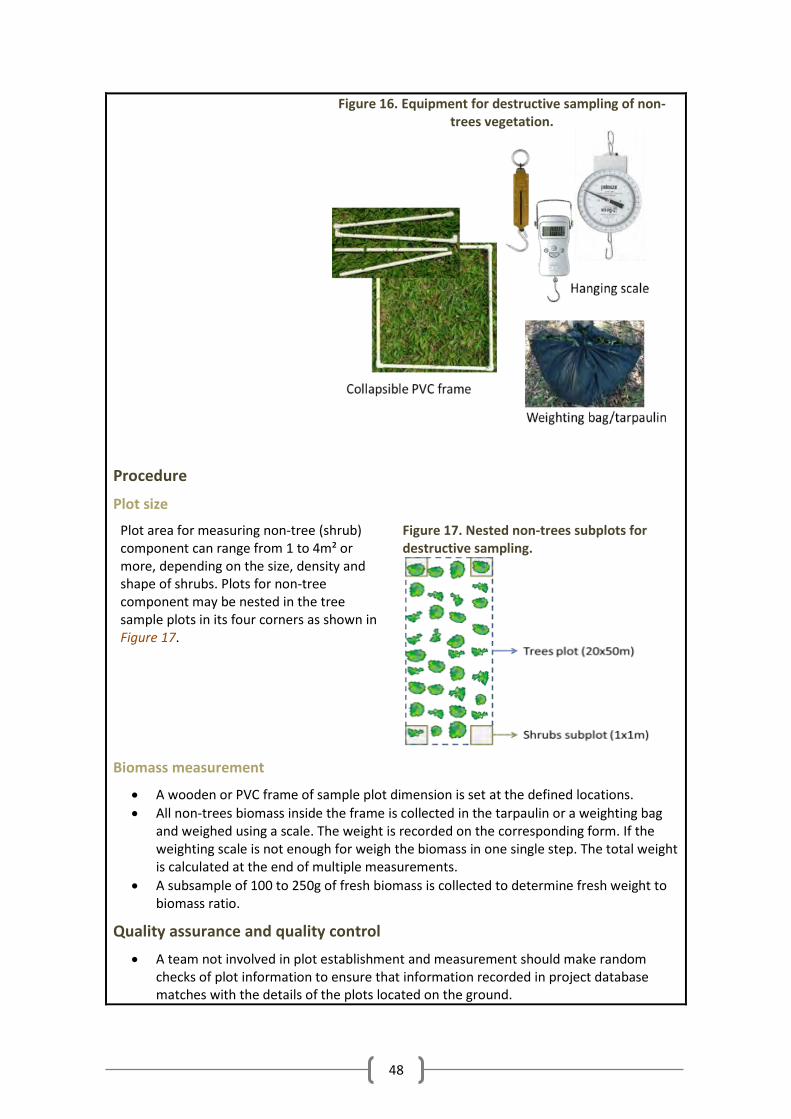
48

Figure 16. Equipment for destructive sampling of non-trees vegetation.

Procedure

Plot size

Plot area for measuring non-tree (shrub) component can range from 1 to 4m² or more, depending on the size, density and shape of shrubs. Plots for non-tree component may be nested in the tree sample plots in its four corners as shown in Figure 17.

Figure 17. Nested non-trees subplots for destructive sampling.

Biomass measurement

A wooden or PVC frame of sample plot dimension is set at the defined locations.

All non-trees biomass inside the frame is collected in the tarpaulin or a weighting bag and weighed using a scale. The weight is recorded on the corresponding form. If the weighting scale is not enough for weigh the biomass in one single step. The total weight is calculated at the end of multiple measurements.

A subsample of 100 to 250g of fresh biomass is collected to determine fresh weight to biomass ratio.

Quality assurance and quality control

A team not involved in plot establishment and measurement should make random checks of plot information to ensure that information recorded in project database matches with the details of the plots located on the ground.

49

The monitoring procedures of non-tree biomass should be as per the procedures of the PDD and the selected methodology.

6.3.1.2 Non-destructive method

Methods for measuring non-tree component in sample plots using non-destructive method are described in the following SOP. Non-destructive method is preferred in cases where non-tree biomass is comprises shrubs that resemble small trees.

SOP 15 - Sampling shrub biomass using non-destructive method

Standard operating procedure for sampling shrub biomass using non-destructive method

Purpose

To describe the process for measuring non-tree (shrub) biomass in sample plots using non-destructive method as part of the monitoring of a CDM A/R project.

Non-trees aboveground biomass is measured for the purpose of calculating carbon stocks changes prior to verification.

Scope

This SOP is relevant for the monitoring staff in charge of monitoring carbon stocks in the field.

Prerequisites

Establishment of permanent tree sample plots (see SOP 12- Establishment of permanent tree sample plots).

Equipment

Diameter tape, F-caliper or C-caliper.

If measuring heights, telescoping measuring rod.

Metric tape.

Figure 18. Equipment for non-destructive sampling of non-tree vegetation.

Procedure

Plot size

50

Plots for nondestructive sampling should contain at least 10 measurable shrubs, and the plots may be nested inside the permanent tree sample plots as shown in Figure 19.

Figure 19. An example of nested shrubs plot for non-destructive sampling.

Biomass measurement

The boundary of the sample plot is fixed inside the tree sample plots (e.g. at the center or at a corner).

The variables necessary for calculating non-tree biomass, e.g., Db (diameter at base), Db and height, Number of stems and height, Dc (crown diameter), Dc and height, etc. should be measured to relate the non-tree biomass and relevant variables as per the allometric model adopted for the purpose

The variables measured should suffice to calculate total (or aboveground) non-trees biomass by applying an allometric model, and optionally a biomass expansion factor suitable for the non-tree vegetation can also be used.

Quality assurance and quality control

The staff not involved in plot establishment or measurement should make random checks of non-tree biomass plots in the field and the data collected on field forms to ensure that data recorded matches with the details of the plots located on the ground.

The staff should also check that the information is correctly processed and the codes for discrete areas and strata are correctly reported.

The equipment used in measurement, including its calibration should be checked to ensure the compliance of monitoring practices as per the requirements of the applicable methodology and procedures outlined in the PDD.

6.4 Dead wood

Deadwood in forest plantations comprises two components – standing deadwood and lying dead wood. Considering the differences in two components, different sampling and estimation procedures should be used to calculate the changes in deadwood biomass of the two components.

6.4.1 Standing dead wood

Standing dead trees are measured on permanent sample plots (established for estimating tree biomass , see Section 6.2- Live trees above) using the same criteria and monitoring frequency

51

used for measuring live trees. The dead/decomposed portion of above-ground and below-ground biomass of standing deadwood is discounted.

The decomposition class of the dead tree and the diameter at breast height shall be recorded and the standing dead wood is categorized under the following four decomposition classes: 1.- Trees with branches and twigs that resemble a live tree (except for leaves) 2.- Trees with no twigs, but with persistent small and large branches 3.- Trees with large branches only and 4.- Boles only, no branches.

For trees in the decomposition class 1 biomass should be estimated using the allometric equation for live trees. When the boles are in decomposition classes 2, 3 or 4, it is recommended to limit the estimation of the biomass to the main trunk of the tree. Usually, there are no allometric equations applicable for such boles and their biomass is estimated based on volume assessment. The volume of dead wood is converted to biomass using the dead wood density appropriate for the decomposition class.

6.4.2 Lying dead wood

Lying deadwood observed on the ground needs to be measured using transect method. Additionally, deadwood also occurs below the ground, which has different rates of decomposition in comparison to the decomposition rates of standing and lying deadwood. As the below-ground deadwood of AR CDM project activities is expected to contribute to the increases in carbon stocks, it may be conservatively omitted from calculations in a CDM forest project.

6.4.2.1 Field procedure

Lying deadwood is monitored using a transect method requires both field and laboratory procedures. The procedure for monitoring lying dead wood is explained in the following SOP.

SOP 16 - Sampling lying deadwood – field procedure

Standard operating procedure for sampling lying deadwood in the field

Purpose

To describe the process for sampling lying deadwood in the field as part of the monitoring of a CDM A/R project.

Lying deadwood is measured for calculating carbon stocks prior to verification.

Scope

This SOP is relevant for the monitoring staff in charge of monitoring carbon stocks in the field.

Prerequisites

Establishment of permanent tree sample plots (see SOP 12- Establishment of permanent tree sample plots).

Equipment

Diameter tape

50 m rope or metric tape

Compass

Figure 20. Equipment for sampling lying deadwood.

52

Machete

Plastic bags and permanent marker

Procedure

Plot size and location

Lying dead wood is measured along two perpendicular transects 50 m each, centered in tree plot, either in N-S and W-E direction, or in the direction of tree plots if tree rows are not N-S or W-E oriented (See Figure 21).

Figure 21. Location of lying deadwood transects.

Measurement of plot

Locate the center of tree plot. With the compass, locate the North-South direction or, locate a direction parallel to the tree rows. Measure a 50 m transect in this direction from the center of plot (25m towards North and 25m towards South).

Measure all pieces of wood (boles or branches) with 5 cm diameter or more at the intersecting point (You only need to measure this diameter, nothing else).

53

Determine density state. Strike the wood with a “machete”. If the blade bounces off, it is sound (S), if it enters slightly is it intermediate (I), and if it causes the wood to fall apart it is rotten (R)

Sample collection for laboratory test

Take at least 10 pieces of wood from each density state (sound, intermediate, rotten), put them in plastic bags.

Identify these samples with density state and plot ID. Samples from different transects may be taken provided all samples are located in the same stratum.

Quality assurance and quality control

A predefined percentage of the sample plots (e.g. 10%) that are measured should be visited in the field and the sample plots re-measured to check the quality of the accomplished activities. If calculated carbon stocks of the re-measured plots differ by more than 10% in comparison to prior measurements of the sample plots, then a full re-measurement of lying deadwood samples must be conducted in the stratum.

6.4.2.2 Laboratory procedure

After measuring lying deadwood in the field and collecting wood samples, a laboratory procedure for determining average wood density for decomposition state of the lying deadwood is required. This procedure was explained in SOP 4- Laboratory wood density determination.

6.5 Litter sample plots

6.5.1.1 Description

Litter includes all non-living biomass with a diameter less than the minimum tree diameter chosen measurement (for example 5 cm) in various states of decomposition on the soil.

Monitoring of litter is similar to the monitoring of non-trees biomass and is explained in the following SOP.

SOP 17 - Sampling litter

Standard operating procedure for sampling litter

Purpose

To describe the process for measuring litter sample plots using destructive methods as part of

54

the monitoring of a CDM A/R project.

Scope

This SOP is relevant for the monitoring staff in charge of monitoring carbon stocks in the field.

Prerequisites

Establishment of permanent tree sample plots (see SOP 12- Establishment of permanent tree sample plots).

Equipment

PVC or wooden frame, metric tape and compass

Weighing scale

Tarpaulin or weighting bag

Figure 22. Equipment for litter sampling.

Procedure

Plot size

Litter plots are nested inside permanent trees plots and may be at fixed or random location.

Figure 23 is an example of subplots systematically located in the four corners of a trees plot.

Size of litter plots can be between 0.5 and 1.0 m² or more, if there is variability in litter distribution. Plots may be square, rectangular or circular and can be delimited using PVC or wood frames of appropriate size. There may be only one big litter plot per tree plot or several smaller sub-plots. Several sub-plots will better represent the variability of litter distribution in comparison to one large plot.

Figure 23. Litter plots location.

Litter measurement

55

The PVC or wooden frame is at the defined locations.

All litter inside the sampling frame is collected, weighed and total fresh weight is recorded on the corresponding field form.

A sub-sample (≈100-250g) of litter is collected in a plastic bag and the sample information is marked on the plastic bag.

The sample collection is repeated for the other 3 sampling frames, and sub-samples are mixed in the same bag (the bag will have a mix of litter from 4 sampling frames).

Total fresh weight of collected litter is recorded.

The litter sample is taken to laboratory and is oven dried until constant weight observed. The dry weight is recorded.

Quality assurance and quality control

Review all data for consistency and check that the forms have no missing information.

Randomly select 10% of the laboratory samples and recalculate their dry weights.

6.6 Soil Organic Carbon

In most soils (with the exception of calcareous soils) the majority of carbon is in the form of soil organic carbon (SOC), and it is expected to increase under the forestry activity in all categories of degraded lands due to a reduction in soil erosion, improvement in soil physical properties, and increases in dead wood and litter from increased vegetation density. The measurable changes in soil organic carbon can be observed after 15–20 years of stand growth. The major variables that influence soil organic carbon include soil depth, bulk density, and concentration of organic carbon.

The changes in soil organic carbon can be assessed by comparing research and published data on non-forested and forested lands in the project area or by conducting sample measurements to estimate the soil organic carbon in the project.

The following SOP describes the procedure for field sampling of soil organic carbon.

SOP 18 - Sampling soil organic carbon

Standard operating procedure for sampling soil organic carbon

Purpose

To describe the process for sampling soil organic carbon as part of the monitoring of an A/R project.

Scope

This SOP is relevant for the monitoring staff in charge of monitoring carbon stocks in the field.

Prerequisites

Establishment of permanent tree sample plots (see SOP 12- Establishment of permanent tree sample plots).

Equipment

Soil corer (optional: soil auger and 2mm test sieve)

Rubber mallet and piece

Figure 24. Equipment for soil organic carbon sampling.

56

of wood

Shovel

Plastic sealable bags

Permanent marker

Procedure

Location of sampling sites

There is no specific location defined for taking soil samples for estimating soil organic carbon. However, it is recommended to collect soil samples systematically in the tree sample plots. A possible arrangement for collecting SOC samples is presented in Figure 25.

Figure 25. Sampling location for soil organic carbon and bulk density samples.

Bulk density sampling

A small pit of 40 cm depth is made so as to insert the soil corer in one of the pit walls at 30 cm depth, pushing with the hand or using a rubber mallet (if required). Push the soil corer into the side of the horizon. If it is difficult to push the corer into the soil, place the piece of wood over the corer and hit the wood with a hammer. This spreads the force of the hammer to all edges of the corer and minimizes bending the corer. If the sides of the corer become bent, this will change its volume and may compact the soil sample, affecting the measurement results. If the sides of the corer bend beyond perpendicular, discard it and use another. Be careful not to compact the soil inside the corer by hammering forcefully.

Using a knife, a trowel or shovel, the soil around the corer is dug to remove it. The soil from the top and the bottom of the corer is trimmed around the edges so that the volume of the soil is the same as the volume of the corer.

The sample is placed in a bag and using knife the entire sample is placed into a plastic bag and it is sealed and labeled.

Bulk density test for gravelly and rocky soils

This method is to be used when rocks or gravels prevent collection of samples for bulk density assessment using the core method described above. This method will require the user to sieve the coarse material greater than 2 mm in size.

57

Materials and equipment

Plastic wrap

140-cc syringe

Water

Garden trowel

Sealable bags and marker pen

2-mm sieve

Scale (0.1 g precision)

1/8-cup (30 mL) measuring scoop

Paper cup or bowl

Access to a microwave oven

Procedure

Choose a spot that is as level as possible to allow water to fill the hole evenly. If the soil is too wet to sieve, ignore the part in Step 2 about replacing rocks, and proceed to Step 3.

Soil will have to be dried and sieved later. The volume of gravel will need to be determined and subtracted from the total volume of the soil sample taken in the field.

Dig a bowl shaped hole three inches deep and approximately twelve centimeters in diameter using the trowel. Avoid compacting the soil in the hole while digging. Place all of the soil and gravel removed from the hole in a plastic bag.

Using the 2-mm sieve, sieve the soil in the plastic bag to separate the gravel. Collect the soil in a plastic sealable bag. Put the gravel aside to be used in Step 2. Seal and label the plastic bag.

Line the hole with plastic wrap to make a tiny pool. Leave some excess plastic wrap around the edge of the hole. Place the sieved rocks and gravel carefully in the center of the hole on top of the plastic wrap. Assure that the pile of rocks do not protrude above the level of the soil surface.

Use the 140 cc syringe to keep track of how much water is needed to fill the lined hole. The level of the water should be even with the soil surface. The amount of water represents the volume of soil removed. Record the total amount of water in cubic centimeters (1 cc = 1 cm³).

Laboratory procedure (both methods)

Weigh the soil sample in its bag. Weigh an empty plastic bag of the same type to account for the weight of the bag, subtract it from total and record it as the sample weight.

Mix sample thoroughly in the bag by kneading it with your fingers. Take a subsample of loose soil (not packed down, approximately one cubic centimeter) from the plastic bag and place it in a paper cup (a glass or ceramic cup may be used).

Weigh the soil subsample in its paper cup. Enter the weight on the soil data worksheet. Weigh an empty paper cup to account for its weight and subtract its weight from the sample weight. Place the paper cup containing the subsample in a microwave and dry for two or more four minute cycles at full power. Open the microwave door for one minute between cycles to allow venting. Weigh the dry subsample in its paper cup and record it.

NOTE: To determine if the soil is dry, weigh the sample and record its weight after each 4-minute cycle. When its weight does not change after a drying cycle, then it is dry.

Calculation

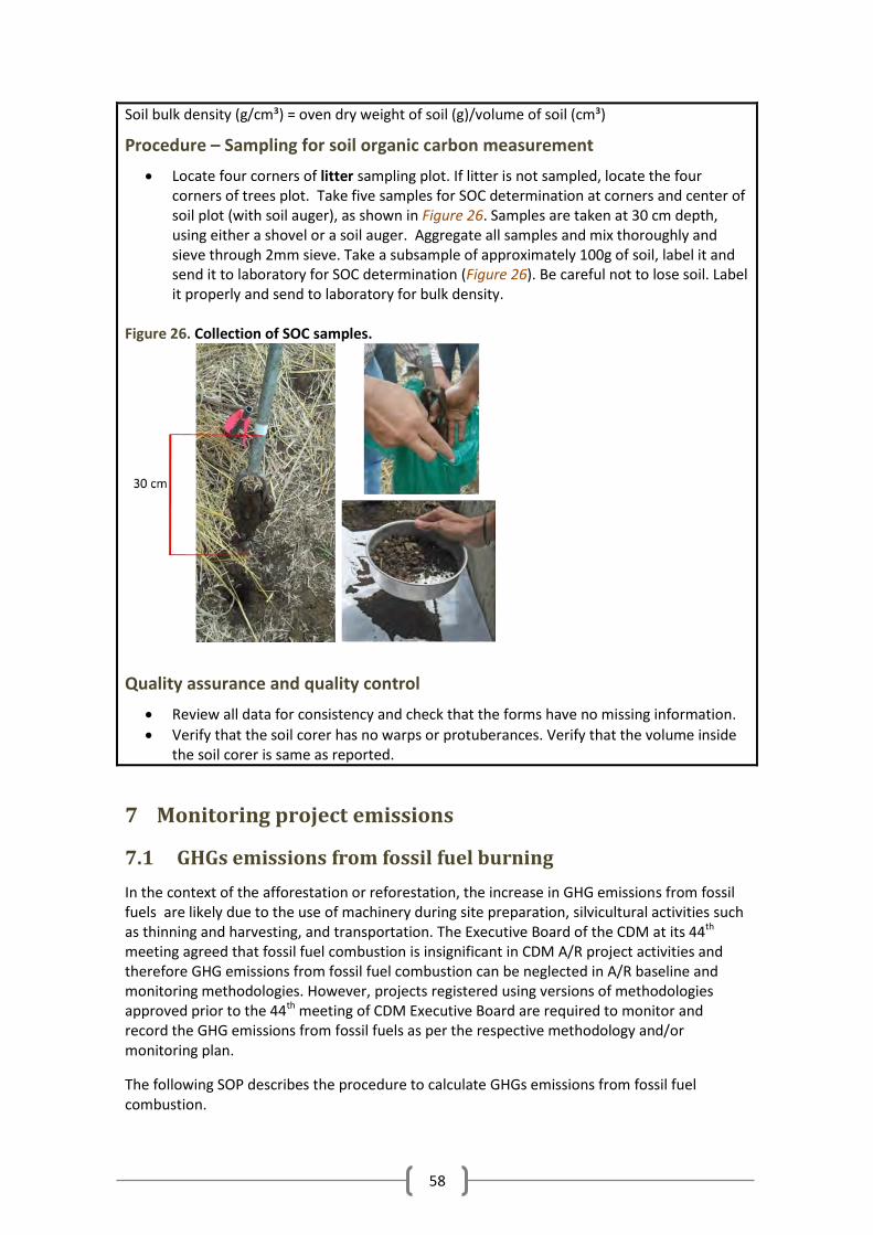
58

Soil bulk density (g/cm³) = oven dry weight of soil (g)/volume of soil (cm³)

Procedure – Sampling for soil organic carbon measurement

Locate four corners of litter sampling plot. If litter is not sampled, locate the four corners of trees plot. Take five samples for SOC determination at corners and center of soil plot (with soil auger), as shown in Figure 26. Samples are taken at 30 cm depth, using either a shovel or a soil auger. Aggregate all samples and mix thoroughly and sieve through 2mm sieve. Take a subsample of approximately 100g of soil, label it and send it to laboratory for SOC determination (Figure 26). Be careful not to lose soil. Label it properly and send to laboratory for bulk density.

Figure 26. Collection of SOC samples.

Quality assurance and quality control

Review all data for consistency and check that the forms have no missing information.

Verify that the soil corer has no warps or protuberances. Verify that the volume inside the soil corer is same as reported.

7 Monitoring project emissions

7.1 GHGs emissions from fossil fuel burning

In the context of the afforestation or reforestation, the increase in GHG emissions from fossil fuels are likely due to the use of machinery during site preparation, silvicultural activities such as thinning and harvesting, and transportation. The Executive Board of the CDM at its 44th meeting agreed that fossil fuel combustion is insignificant in CDM A/R project activities and therefore GHG emissions from fossil fuel combustion can be neglected in A/R baseline and monitoring methodologies. However, projects registered using versions of methodologies approved prior to the 44th meeting of CDM Executive Board are required to monitor and record the GHG emissions from fossil fuels as per the respective methodology and/or monitoring plan.

The following SOP describes the procedure to calculate GHGs emissions from fossil fuel combustion.

59

SOP 19 - Monitoring GHGs emissions from fossil fuel combustion

Standard operating procedure for monitoring GHGs emissions from fossil fuel combustion

Purpose

To describe the process for collecting data for monitoring GHGs emissions from fossil fuel combustion.

Scope

This procedure is intended for staff in charge of monitoring project emissions of CDM A/R activities.

Prerequisites

None.

Requirements

No special equipment is required

Procedure

Step 1: Monitoring the type and amount of fossil fuels consumed. The type of fossil fuels (diesel, gasoline) and amount of consumption for project activities such as site preparation, thinning and harvesting needs to be recorded. According to the decision of Executive Board at its 42nd meeting, monitoring of fossil fuel consumption from transportation is not required.

Option 1: Direct method. Total fossil fuels consumption can be established from annual fuel bill, separated by fuel type (e.g. if project has machinery in use and can track expenses related to fuel consumption of the machinery).

When using this method, fuel consumption can be monitored using the fuel bill or tracking each vehicle or equipment separately.

If Option 1 is used, supporting evidence on the purchase and use should be recorded monthly or annually to calculate the total quantity of fossil fuel consumed over the monitoring period.

Option 2: Indirect method. Fossil fuel consumption is calculated based on machinery use and fuel efficiency. Machinery use is tracked according to the nature of the operation (e.g. hours of machine use times the average fuel consumption per hour; traveled kilometers times average fuel consumption per traveled kilometer; cubic meters harvested times the average fuel consumption per cubic meter, etc.).

Indirect method estimates fuel consumption from parameters other than fuel bills or tracking fuel amounts, e.g. by tracking amount of harvested wood, duration of machinery or equipment use, distance traveled, etc.

In this option, parameters for converting time of use of machinery and equipment must be noted in order to convert the variable (e.g. time of use of machinery or equipment, amount of wood, area prepared or planted, etc.) into amount of fuel consumed. The conversion factors may be developed by sampling corresponding activities to determine fuel efficiency per unit of activity involving fossil fuel consumption.

After the parameters for estimating fuel consumption per unit are assessed, field operations requiring the use of fuels are monitored to estimate the fossil fuel consumption.

As an example, if it is determined by sampling that mechanical weed control consumes

60

0.96 liters of gasoline per hectare, weed control of 236 ha of plantations will require 236 x 0.96 =226.56 liters of gasoline. Then Step 2 may be applied to this value.

Step 2: Choosing emission factors. There are three possible sources of emission factors:

National emission factors: These emission factors may be developed by national programs such as national GHG inventory;

Regional emission factors;

IPCC default emission factors are used when no information on emission factors is available.

Step 3: Calculating emissions. The quantity of each type of consumed fossil fuel consumed is multiplied with the corresponding emission factor to calculate GHG emissions from the respective fossil fuel. This calculation should be done for each type of fossil fuel, and for all years of the monitoring period.

Quality assurance and quality control

Review all data for consistency and check that the forms have no missing information.

Fuel consumption data is cross checked against other sources of project information.

Verify that reported figures are reasonable for the type of project activity monitored.

7.2 GHGs emissions from biomass burning

Biomass burning is a source of GHG emissions in an A/R project and it results in CO2, CH4 and N2O emissions.

There are several methods for monitoring and estimating GHG emissions from biomass burning in approved methodologies. All of them require monitoring of burnt areas and estimation aboveground biomass stock prior to burning. Some of them require monitoring pre-existing biomass of trees, shrubs and herbs separately, while others use total pre-existing biomass for calculations.

The carbon stocks are converted into corresponding GHG taking into account combustion efficiencies and conversion factors.

The following SOP describes the procedure to calculate GHG emissions from biomass burning.

SOP 20 - Monitoring GHGs emissions from biomass burning

Standard operating procedure for monitoring GHGs emissions from biomass burning

Purpose

To describe the process of data collection for monitoring GHG emissions from biomass burning.

Scope

This procedure is intended for staff in-charge of monitoring emissions from AR CDM project activities.

61

Prerequisites

None.

Requirements

Maps

GPS receiver

Field data forms

If field sampling of carbon stocks is required, see Section 6 on monitoring of carbon stocks.

Procedure for data collection (all approaches)

It is very important to monitor biomass burning in a timely fashion, i.e., collecting all required data when biomass is burnt as part of site preparation or in forest fires. The area burnt and date of biomass burn must be recorded. If biomass burning occurs over a large area or dispersed over several discrete areas, sampling of areas burnt and areas that are not burnt may need to be done to estimate the GHG emissions from biomass burning (review the procedures of applicable methodology) following procedures described in Section 6.

Procedure – standard approach

Step 1. Measuring and estimating the above- and below-ground biomass of existing non-tree vegetation. Majority of approved CDM A/R methodologies require estimation of biomass subject to burn using sampling approach. The herbaceous plants and/or shrubs can be measured by simple harvesting techniques or by non-destructive methods, using allometric models (see Section 6.3 above). One methodology (AR-AM0010) allows the use of ex-ante estimation of the existing non-tree biomass.

Step 2. Estimating GHG emissions from biomass burning. For this estimation, it is required to estimate combustion efficiencies and emission factors. The combustion efficiencies may be chosen from Table 3.A.14 of GPG-LULUCF (see ancillary tool IPCC - 2003 - GPG for LULUCF Tables.xls). If appropriate combustion efficiency data is not available, the IPCC default of 0.5 should be used. The nitrogen-carbon ratio (N/C ratio) is approximated to be about 0.01. This is a general default value that applies to leaf litter, but lower values would be appropriate for woody biomass, if data are available. Emission factors for use with equations are provided in Tables 3.A 15 and 3.A.16 of GPG-LULUCF (see ancillary tool IPCC - 2003 - GPG for LULUCF Tables.xls).

Procedure – Methodological tool

The CDM Executive Board published a methodological tool for the estimation of GHG emissions due to clearing, burning and decay of existing vegetation attributable to a CDM A/R project activity. This tool can be used to estimate the increase in GHG emissions due to live woody vegetation in the A/R project boundary. Following is a summary of the steps for calculating GHG emissions from the burning of biomass according to this tool.

Step 1. Measuring or estimating the above- and below-ground biomass of existing vegetation. This estimation must be done separately for existing trees (if any), shrubs (if any) and herbs. If lands within the project area have a history of periodic clearance of existing vegetation by fire or felling, estimation of emissions due to site preparation may be based on the average levels of biomass present over multiple fire/felling cycles. If this history does not exist, field sampling (as explained for the standard approach) must be used.

Step 2. Measuring burnt areas. Identification of burnt areas, date of burn and areas

62

burnt must be measured and recorded, and area burnt is used to estimate GHG emissions from biomass burning.

Step 3. Estimating GHG emissions from biomass burning. For this estimation, it is required to estimate combustion efficiencies and emission factors. For this approach, the values in Table 2 are used.

Table 2. Conservative default factors for biomass burn emissions calculation.

Factor Value Description

Cftree 0.50 t C/(t d.m.) Average carbon fraction of biomass for tree vegetation

Cfshrub 0.49 t C/(t d.m.) Average carbon fraction of biomass for shrub vegetation

fBLtree 0.4 The fraction of biomass of tree vegetation left to decay after burning

fBLshrub 0.05 The fraction of biomass of shrub vegetation left to decay after burning

Rtree 0.3 Average root:shoot ratio appropriate for biomass stocks, for tree vegetation

Rshrub 0.4 Average root:shoot ratio appropriate for biomass stocks, for shrub vegetation

Quality assurance and quality control

Review all data for consistency and check that the forms have no missing information.

Cross check the information with other departments of the project (e.g. the management department or section, or the forest protection unit, if any) to verify the consistency of the reported forest fires with the other sources of information.

Check at random some of the reported fires by visiting the area affected by fire. Check that the reported figures are supported with the evidence observed in the field.

7.3 GHGs emissions from the use of fertilizers

GHG emissions from the use of fertilizers are carbon dioxide (CO2), nitrous oxide (N2O) and methane (CH4). The CDM Executive Board at its 42nd meeting agreed that emissions from fertilizer application may be considered as insignificant and hence can be neglected in A/R baseline and monitoring methodologies and tools. However, the projects registered prior to the EB decision need to comply with the versions of approved methodologies that require the monitoring of N2O emissions from nitrogen fertilization.

The two kinds of nitrogen fertilizers considered as a source of GHG emissions in forestry projects are organic and chemical. The following SOP describes the procedure to calculate GHGs emissions from the use of fertilizers in an A/R project activity.

SOP 21 - Monitoring GHGs emissions from fertilizer use

Standard operating procedure for monitoring emissions from fertilizer use

Purpose

To describe the process for collecting data for monitoring GHGs emissions from fertilizer use.

Scope

This procedure is intended for staff in charge of monitoring project emissions in AR activity.

63

Prerequisites

None.

Requirements

No specific requirements.

Procedure

Quantities and nitrogen content of synthetic and organic fertilizers are monitored and recorded.

For each kind of fertilizer used in the project, a unique identification code is assigned and new fertilizer code is used if fabrication batches of fertilizer differ from previous ones and nitrogen content as percentage of total fertilizer is recorded.

For each purchase of chemical or organic fertilizer, purchase or fabrication date, invoice code, fertilizer ID, fertilizer type, quantity and units are recorded.

How to determine N content

All fertilizer labels have a label (fertilizer grade) with (at least) three bold numbers, representing the primary nutrients:

First : percentage of nitrogen (N)

Second: percentage of phosphate (P2O5)

Third: percentage of potash (K2O).

Example: a bag of 10-22-31 fertilizer contains 10 percent nitrogen, 22 percent phosphate and 31 percent potash. To calculate the amount of Nitrogen of a fertilizer, multiply the weight of fertilizer by the percentage of nitrogen in the fertilizer grade. Example: 50 kg of 10-22-31 fertilizer contain 50*10/100 = 5 k of nitrogen

Quality assurance and quality control

Review all data for consistency and check that the forms have no missing information.

Fertilizer use data are cross checked against relevant project information (e.g. report on forest establishment, silvicultural activities etc.).

64

8 Monitoring Leakage

For CDM A/R project activities, leakage can be defined as the net GHGs emission which occurs outside the project boundary, and which is measurable and attributable to the CDM project activity. The types of leakage considered in A/R methodologies are: grazing displacement, displacement of pre-project crop cultivation activities, displacement of fuel wood collection activities and use of wood from non-renewable biomass for fencing.

8.1 GHGs emissions from grazing displacement

In the case of grazing displacement, leakage may occur if as grazing activities are displaced to areas outside the project. Grazing activities displaced to other existing grazing land or forest areas or unidentified areas and need to be monitored. The leakage due to grazing displacement is relevant for a period of 5 years from the period when measures are implemented to address it after the project start date. Therefore, assessment of leakage due to grazing displacement is relevant during the first monitoring period.

8.1.1 Data collection

CDM A/R methodologies dealing with grazing displacement have adopted different methods to account for the leakage related to grazing displacement. The early versions of A/R methodologies (e.g., AR AM0003, AR AM0004) included leakage assessment procedures that require collection of data pertaining to grazing displacement in different types of land. As a consequence, the leakage assessment in projects using these methodologies is time intensive. The example of assessing grazing leakage in projects using AR AM0003 and AR AM0004 methodologies is presented in Box 2 below.

To assess grazing displacement in projects that use methodologies (e.g., AR ACM0001, AR AM0005 and AR AM0013), the projects should consult “Guidelines on conditions under which increase in GHG emissions related to displacement of pre-project grazing activities in A/R CDM project activity is insignificant” (EB 51, Annex 13) to demonstrate that increase in emissions of greenhouse gases due to displacement of pre-project grazing activities attributable to the A/R CDM project activity is insignificant and may be accounted as zero.

If as per the above guidelines, the increase in GHG emissions from due to displacement of pre-project grazing activities cannot be considered insignificant, the project should use the latest version of methodological tool, “Estimation of the increase in GHG emissions attributable to displacement of pre-project agricultural activities in A/R CDM project activity” (EB 51, Annex 15) to calculate the leakage associated with the displacement of pre-project agricultural activities.

Box 2. Example of assessing grazing displacement in projects using the procedures of methodologies - AR AM0003, AR AM0004.

The following paragraphs describe the data required for estimation of leakage from grazing displacement and methods for data collection along with an example of leakage calculation. Estimation of pre-project animal population in project area (NaBL): This can obtained from the registered PDD. Estimation of animal population supported by project area (NaAR): The estimation of this

65

value depends on the characteristics of the project. If the fodder production increase as a result of the project supports more livestock relative to the baseline scenario, then no leakage is expected to occur and the leakage from grazing displacement is treated as zero. The data on fodder production on farm and the area available for grazing and the time period of grazing within the project area can be obtained from project statistics or from surveys of landowners participating in the project. In case the project covers community lands, sample survey of households participating in the project can be used to assess the animal units supported by the fodder production within the project area. Estimation of existing grazing lands outside the project to which the animals are displaced (EGL) and current animal population in the EGL: If the livestock is displaced to existing grazing lands (e.g., village common lands) in the region outside the project, the area of existing grazing lands, number of livestock grazing on these lands, months of grazing, and carrying capacity of the lands to support grazing need to be collected. The data can be collected from a survey of 10% project households on whether or not they use the EGL, The data on the extent of EGL, number of animals grazed and time period of grazing during a year are collected from information on land use recorded at the local level. In addition to EGL, if the livestock is displaced to new grazing land (NGL) and unidentified grazing land (XGL) areas, procedures similar to those followed in assessing the grazing displacement in EGL need to be followed in NGL and XGL areas. Baseline scenario/Pre project situation: There are 788 livestock units prior to the start of the project. Therefore, Estimated pre-project animal population in project area (NaBL): 788 (recorded in the PDD). Project scenario: The 44 households participating households implement A/R project on 747.1 ha. To monitor leakage due to grazing displacement, 10 percent of project households (i.e., 4 out of 44 households) are randomly selected for survey during the first monitoring period prior to verification. Percentage of sampled households: 4/44= 10.81% Table 3. Livestock units supported by the project.

Land owner Project area (ha) Animal units supported by the project area (grazing and fodder production)

John Doe 5.5 5

Juanita Doe 52.8 36

Junior Doe 12.5 11

Jane Doe 13.1 14

Total 83.9 66

Based on the sample survey, Fraction of project area sampled for animal grazing: 83.9/747.1 = 0.11 Sampled number of livestock units supported by the project: 66 Number of livestock supported by the project (NaAR): 66/0.11 = 600 Number of livestock units displaced to EGL: 788 - 600 = 188.

66

Area of existing grazing land (EGL) outside project (from land use records of village/commune) = 1455.5 ha Carrying capacity of EGL in number of animals (@ 1.5 animals/ha/year) = 2183.25 Number of village/commune livestock units grazing on EGL prior to project (at time t-1, based on survey or official record)= 1379 units Number of livestock units grazing on EGL after project implementation (at time t, based on survey) = 1717 dNaEGLt = 1717 – 1379 = 338 (includes 188 livestock units displaced from project area) = NaBL < NaAR + dNaEGLt

= 788 < 600 + 388 As NaBL < NaAR + dNaEGLt, livestock units displaced due to the AR CDM project activity does not lead to leakage.

8.2 GHG emissions from displacement of pre-project crop cultivation activities

To assess displacement of pre-project crop cultivation activities in projects that use methodologies (e.g., AR ACM0001, AR AM0011, AR AM0013), the projects should consult “Guidelines on conditions under which increase in GHG emissions related to displacement of pre-project crop cultivation activities in A/R CDM project activity is insignificant” (EB 51, Annex 14) to demonstrate that increase in emissions of greenhouse gases due to displacement of pre-project crop cultivation activities attributable to the A/R CDM project activity is insignificant and may be accounted as zero.

If as per the above guidelines, the increase in GHG emissions from due to displacement of pre-project grazing activities cannot be considered insignificant, the project should use the latest version of methodological tool, “Estimation of the increase in GHG emissions attributable to displacement of pre-project agricultural activities in A/R CDM project activity” (EB 51, Annex 15) to calculate the leakage associated with the displacement of pre-project agricultural activities.

8.3 GHGs emissions from fuel wood collection displacement

8.3.1 Description

The increase in GHG emissions associated with the displacement of fuel-wood collection as a result of the accounted in some methodologies (e.g., AR AM0003, AR AM0004).

The leakage due to fuelwood collect is zero if, leakage due to displacement of fuel-wood collection can be set as zero (LK fuel-wood = 0) under the following conditions:

• FGBL < FGAR,t;

• LK fuel-wood < 2% of actual net GHG removals by sinks

Where,

FGBL = Average pre-project annual volume of fuel-wood gathering in the project area; m3 yr-1

67

FGAR,t = Volume of fuel-wood gathering allowed/planned in the project area under the proposed AR CDM project activity; m3 yr-1

The condition FGBL < FGAR,t; states that if the fuel wood production in the CDM A/R project is greater than the fuel wood collection in the baseline, then the leakage due to displacement of fuel-wood collection is zero

The pre-project consumption of fuel-wood can be assessed by interviewing randomly selected households through Participatory Rural Appraisal (PRA) or survey methods. The “General Guidelines for Sampling and Survey for Small Scale CDM project activities, Version 01 (EB50, Annex 30) are to be consulted if survey methods are used. The local studies on fuel-wood consumption and/or charcoal production may also be used.

In situations where leakage due to displacement of fuel-wood collection is not zero (FGoutside,t = FGBL > FGAR,t); then the following SOP describes the procedure to assess GHG emissions from displacement of fuel wood collection.

SOP 22 - Monitoring of GHGs emissions from fuel wood collection displacement

Standard Operating Procedure for monitoring GHGs emissions from fuel wood collection displacement

Purpose

To describe the process of data collection for monitoring of GHG emissions from the displacement of fuel wood collection as a consequence of the implementation of AR CDM project activities.

Scope

This procedure is intended for staff in charge of monitoring project emissions as part of the monitoring process of AR CDM project activities.

Prerequisites

Monitoring of project boundaries.

Requirements

No specific equipment required.

Procedure

Step 1: Assess the average fuel wood collection in the project area in order to estimate the volume of fuel wood collection displaced outside the project boundary. Monitoring can be done by interviewing households, through a Participatory Rural Appraisal (PRA) or field sampling. For guidance on how to conduct PRA, see SOP 23 - Participatory Rural Appraisal for estimating fuelwood collection displacement. If survey methods are used, “General Guidelines for Sampling and Survey for Small Scale CDM project activities, Version 01 (EB50, Annex 30) need to be consulted.

Step 2: The volume of fuel wood gathering of pre-project fuel wood collectors or charcoal producers in new grazing lands (NGL) outside the project to be monitored using PRA or surveys

Leakage due to displacement of fuel wood collection can be assessed as FGt = FGoutside,t – FGNGL, t.

68

Leakage due to displacement of fuel-wood collection is estimated using (IPCC GPG-LULUCF - Equation 3.2.8)

Quality assurance and quality control

Review all data for consistency and check that the forms have no missing information.

Cross check the registered PDD against the reported data.

Verify that the supporting documentation is available and of enough quality for a verification.

SOP 23 - Participatory Rural Appraisal for estimating fuelwood collection displacement

Standard Operating Procedure for conducting a Participatory Rural Appraisal for estimating fuelwood collection displacement

Purpose

Describe the process for conducting a Participatory Rural Appraisal for estimating fuelwood collection displacement through interviews.

Scope

This procedure is intended for monitoring staff involved in quantifying fuelwood collection displacement.

Prerequisites

None.

Requirements

Voice recorder

Pre-designed questionnaire (optional)

Two to four people for conducting interviews

Procedure

Participatory Rural Appraisal is a flexible, short-cut method of data collection that relies heavily on participation by the communities and that can be used among others, for estimating fuelwood collection displacement. The following procedure gives general guidance for one optional method, based on semi-structured interviews that should be suited to specific circumstances.

Designing and planning the interview

The semi-structured interview is an informal, guided interview session, where only some of the questions are pre-determined and new questions arise during the interview, in response to answers from those interviewed. Predetermined questions should be focused on determining for the past and the current situation:

Frequency of fuelwood collection activities

Amount of collected fuelwood

Source location of fuelwood

Seasonality of fuelwood collection activities

Current energy sources.

69

Selecting interviewees

The number of interviewees depends on the extent of the preexisting fuelwood collection activities. The interviewees may be (1) households, (2) key informants, and (3) community groups.

Conducting the interviews

The interviews are conducted by a team of 2 to 4 persons and can be led (moderator) by different people in different occasions.

Moderator will introduce a topic for all the participants to discuss while another member of the team records the information.

Discussions are recorded, transcribed, and translated (if required). Data inferred and or collected from the transcriptions is organized and then the person in charge of data collection carries out the analysis.

Quality assurance and quality control

Transcript notes are read and cross-checked by independent staff.

Recording equipment is checked to determine its reliability.

As PRA-generated data in their original form are seldom conducive to statistical analysis, alternative approaches are based on stratified sampling.

8.3.2 GHGs emissions from use of non-renewable wood for fencing

As per the early version of A/R methodologies, projects that use wood from non-renewable sources for fencing or other uses in project area, need to account GHG emissions as per the guidance of the relevant methodology.

As per the decision of 44th meeting of CDM Executive Board, the leakage associated with the use of wood from non-renewable sources is considered negligible and therefore can be ignored. Therefore, methodologies that have been revised taking into account the decision of 44th meeting of EB need not consider the leakage from this source.

The projects registered using early versions of A/R methodologies (approved prior to EB44 decision) may need to consider the relevance of this leakage.

9 Project level Quality Assurance / Quality Control (QA/QC)

Although Standard Operational Procedures presented in this Operational Manual define Quality Assurance and Quality Control measures specific to each project activity, this section focuses on general QA/QC procedures that should be implemented at project level.

Coordination of monitoring

It is crucial that one or more project personnel coordinate the monitoring activities of a project to interpret the monitoring plan into procedures deployable to field operators. This role needs personnel dedicated to the task, depending on factors such as the degree of integration of the requirements with the existing organization functions, the complexity of project activities and the potential revenue from CERs to justify a dedicated role.

The responsibilities of monitoring coordinator are:

70

Execution of the monitoring, data collection and reporting procedures;

Deployment of the procedures to field staff to ensure that the procedures are fully complied with;

Organization of equipment and devices required for monitoring and data collection;

Conduct of training for project teams on aspects related to monitoring and data collection;

Organization of data for calculation of emission reductions and for monitoring report; and

Interaction with Designed Operational Entity during verification.

Reliability of field measurements

Reliability of field measurements may be improved through the use of SOPs for each step of the field measurements, including provisions of documentation for verification purposes, the implementation of training courses on the field data collection and data analyses for persons involved in the field measurement works. The training courses should ensure that field-team members are fully aware of all procedures and the importance of collecting data as accurately as possible. To achieve this, both classroom examination and field examination may be conducted, and only those that have passed the examination can join the team.

Random checks of field data collection. To verify that plots have been installed and the measurements taken correctly, randomly selected plots may be re-measured by teams other than those involved in the prior plot measurements. Key re-measurement elements should include the location of plots, DBH and tree height. The re-measurement data may be compared with the original measurement data. Errors assessed in the prior measurements will be corrected and recorded and would be used to calculate the measurement error.

Checks of data entry and analysis. To minimize possible errors in the process of data entry, the entry of both field data and laboratory data will be reviewed by an independent expert team and compared with independent data to ensure that the data are realistic. Communication between all personnel involved in measuring and analyzing data should be used to resolve any apparent anomalies before the final analysis of the monitoring data is completed.

Data maintenance and archiving. Data archiving should be both electronic and in paper forms, and copies of all data should be provided to each project participant. All electronic data and reports should also be copied on durable media and stored in multiple locations. The archives should include: - Copies of all original field measurement data, laboratory data, data analysis spreadsheets; - Estimates of the carbon stock changes in all pools and non-CO2 GHG and corresponding calculation spreadsheets; - GIS products; - Copies of the measuring and monitoring reports.

It is important to institutionalize the scope of work, reporting line, and routines of the Monitoring Coordinator within the context of the Standard Operational Procedures and the QA/QC procedures of a project, to encourage information sharing among employees whenever there is a rotation of personnel during a crediting period.

71

10 References and useful links

10.1 Publications

IPCC (Intergovernmental Panel On Climate Change), 2003. Good Practice Guidance for Land Use, Land-Use Change and Forestry. Institute for Global Environmental Strategies (IGES), Hayama, Japan. 595p.

IPCC (Intergovernmental Panel On Climate Change), 2006. Guidelines for national greenhouse gas inventories, Volume 4 (Agriculture, Forestry and Other Land Uses). Eds S Eggleston; L Buendía; K Miwa; T Ngara; K Tanabe. IGES, Hayama, JP. 679p.

Walker, S.M., Pearson, T., Brown, S. 2007. Winrock Terrestrial Sampling Calculator. Excel tool freely available at http://www.winrock.org/Ecosystems/tools.asp.

Zomer, Robert; Kägi, Wolfram; Robledo, Carmenza; Muys, Bart 2007. Encofor Fieldwork

Manual. Environment and community based framework for designing afforestation,

reforestation and revegetation projects in the CDM: methodology development and case

studies.

10.2 Useful websites

UNFCCC CDM homepage

Most important source of information. Full CDM regulatory framework .

http://cdm.unfccc.int/

CDM Executive Board

Meeting archives, methodologies, decisions, etc.

/EB/index.html

CDM A/R methodologies (regular and consolidated)

This section provides access to approved methodologies and the methodological tools agreed by the Executive Board.

/methodologies/ARmethodologies/index.html

CDM A/R methodologies (small scale)

Approved small scale CDM A/R methodologies

/methodologies/SSCmethodologies/SSCAR/approved.html

CDM Validation and Verification Manual v.1.1

Executive Board guidance for designated operational entities on verification and validation

/EB/051/eb51_repan03.pdf

IPCC Guides and database

The Intergovernmental Panel on Climate Change has published some guidance to assist in producing accurate carbon inventories at country level. The most important guides for forestry projects are the Lulucf (Land Use, Land Use Change and Forestry) and the Afolu (Agriculture, Forestry and Other Land Use) guides.

GPG LULUCF 2003 *

Good Practice Guidance for Land Use, Land Use Change and Forestry

http://www.ipcc-nggip.iges.or.jp/public/gpglulucf/gpglulucf.html

AFOLU Guidelines 2006 *

72

The Afolu (Agriculture, Forestry and Other Land Uses) Guide is part of the 2006 IPCC Guidelines for National Greenhouse Gas Inventories

http://www.ipcc-nggip.iges.or.jp/public/2006gl/index.html

IPCC Emission Factors Database

A database of emission factors and other parameters with background documentation or technical references that can be used for estimating greenhouse gas emissions and removals.

http://www.ipcc-nggip.iges.or.jp/EFDB/main.php

Winrock - BioCF

Sourcebook for Land Use, Land Use Change and Forestry Projects

http://www.winrock.org/ecosystems/files/Winrock-BioCarbon_Fund_Sourcebook-compressed.pdf

Winrock Terrestrial Sampling Calculator

An Excel file for calculating sampling size (number of required plots ) for baseline and monitoring measurements.

http://www.winrock.org/ecosystems/files/Winrock_Sampling_Calculator.xls

Carbon Decisions

Minga – A database of observed growth data for tropical species and generic growth models

An Excel file for modeling management and productivity of tropical forest species. Includes a database of growth data and many useful parameters for carbon calculations.

http://www.carbondecisions.com/tools/Minga.rar

10.3 GPS Mapping software

ExpertGPS - http://www.expertgps.com/default.asp Mapping software for viewing GPS waypoints and tracklogs from any handheld GPS receiver over aerial photos and US topographic maps. It allows to convert any GPS, GIS, or CAD data to or from GPX, Google Earth KML or KMZ, Excel CSV or TXT, SHP shapefiles, or AutoCAD DXF drawings, reproject data in any geographic format and change datums instantly.

Garmin MapSource -

http://www.garmin.com/garmin/cms/us/maps/tripplanningsoftware/mapsource

Mapping software for creating, viewing, and editing waypoints, routes, and tracks from Garmin

devices.

GPS TrackMaker Free - http://www.gpstm.com/ Free program for creating maps with GPS devices compatible with more than 160 GPS models (support for Garmin, Magellan and others).

OziExplorer GPS Mapping Software - http://www.oziexplorer.com/

Mapping software that works with Magellan, Garmin, Lowrance, Eagle, Brunton/Silva and MLR

GPS receivers for the upload/download of waypoints, routes and tracks and most brand of GPS

receivers for real time tracking of GPS position (Moving Map).

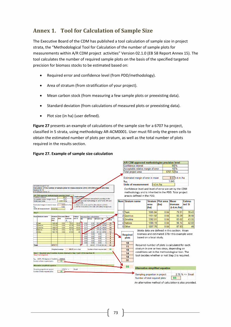
73

Annex 1. Tool for Calculation of Sample Size

The Executive Board of the CDM has published a tool calculation of sample size in project

strata, the “Methodological Tool for Calculation of the number of sample plots for

measurements within A/R CDM project activities” Version 02.1.0 (EB 58 Report Annex 15). The

tool calculates the number of required sample plots on the basis of the specified targeted

precision for biomass stocks to be estimated based on:

Required error and confidence level (from PDD/methodology).

Area of stratum (from stratification of your project).

Mean carbon stock (from measuring a few sample plots or preexisting data).

Standard deviation (from calculations of measured plots or preexisting data).

Plot size (in ha) (user defined).

Figure 27 presents an example of calculations of the sample size for a 6707 ha project,

classified in 5 strata, using methodology AR-ACM0001. User must fill only the green cells to

obtain the estimated number of plots per stratum, as well as the total number of plots

required in the results section.

Figure 27. Example of sample size calculation