manual move3 pdf a4 - purdue engineeringbethel/mv3.pdf · manual move3 @ grontmij geogroep 6 1.1....
TRANSCRIPT

USER MANUALVersion 3.1
© @ Grontmij Geogroep bvAll rights reserved

TrademarksAll brand names and product names mentioned in this document aretrademarks or registered trademarks of their respective companies/owners.
Copyright AcknowledgementThis software product is protected by copyright and all rights are reserved byGrontmij Geogroep bv. Lawful users of this software are licensed to have theprograms read from their medium into the memory of a computer, solely forthe purpose of executing the programs. Copying, duplicating, selling orotherwise distributing this product is a violation of copyright law.This manual is protected by copyright and all rights are reserved.While a great deal of effort has gone into preparing this manual, no liability isaccepted for any omissions or errors contained herein.Grontmij Geogroep makes no representations or warranties with respect tothe contents hereof and specifically disclaims any implied warranties ofmerchantability or fitness for any particular purpose.
Note:Designs and specifications are subject to change without notice.
@ Grontmij Geogroep bvBovendonk 29, P.O. Box 1747, 4700 BS Roosendaal, The Netherlands
Telephone +31-165-575859; Telefax +31-165-561368E-mail [email protected]
http://www.MOVE3.com
Manual MOVE3
@ Grontmij Geogroep 3
Contents1. Getting started 5
1.1. Introduction 61.1.1. General 61.1.2. About this Manual 61.1.3. MOVE3 Specifications 7
1.2. Installation 91.2.1. Package Contents 91.2.2. Hardware and Software Requirements 91.2.3. Installation Procedure 91.2.4. Starting MOVE3 9
1.3. Tutorial 101.3.1. Introduction 101.3.2. Starting and Using MOVE3 for Windows 101.3.3. Projects 101.3.4. Controlling Geometry 121.3.5. Compute 131.3.6. Adjustment in Phases 141.3.7. Closing MOVE3 16
2. Using MOVE3 172.1. Introduction 18
2.1.1. System Overview 182.2. MOVE3 Model 19
2.2.1. General 192.2.2. Observation Types 212.2.3. Dimension Switch and Observation Type 242.2.4. Combining Observations 252.2.5. More information... 27
3. Geodetic Concepts 283.1. Introduction 293.2. Reference Systems 30
3.2.1. General 303.2.2. Global and Local Systems 313.2.3. Geoid and Height Definition 323.2.4. Datum Transformations 34
3.3. Map Projections 363.3.1. Purposes and Methods of Projections 363.3.2. The Transverse Mercator Projection 383.3.3. The Lambert Projection 383.3.4. The Stereographic Projection 393.3.5. The Local (Stereographic) Projection 40
3.4. GPS 413.4.1. General 413.4.2. GPS Observations 413.4.3. GPS in Control Networks 423.4.4. GPS stochastic model 433.4.5. GPS and Heights 43
Contents Manual MOVE3
@ Grontmij Geogroep 4
3.5. Detail Measurements 443.5.1. Geometrical relations 443.5.2. Precision of idealisation 463.5.3. Eccentric measurement 46
4. Quality Control 484.1. Introduction 49
4.1.1. Adjustment, Precision, Reliability and Testing 494.1.2. Quality Control in Network Planning 50
4.2. Least Squares Adjustment 524.2.1. General 524.2.2. Mathematical Model 524.2.3. Stochastic Model 544.2.4. Free and Constrained Adjustments 564.2.5. Formulae 57
4.3. Precision and Reliability 594.3.1. General 594.3.2. Precision 604.3.3. Reliability 61
4.4. Statistical Testing 644.4.1. General 644.4.2. F-test 654.4.3. W-test 664.4.4. T-test 674.4.5. Interpreting Testing Results 684.4.6. Estimated Errors 69
5. Lists 705.1. List of Map Projections and Constants 715.2. Literature List 735.3. MOVE3 File Structures 74
5.3.1. MOVE3 Input Files 745.3.2. MOVE3 Output Files 89
5.4. Glossary 92

Manual MOVE3
@ Grontmij Geogroep 5
1. Getting started
Manual MOVE3
@ Grontmij Geogroep 6
1.1. Introduction
1.1.1. GeneralMOVE3 is a software package developed by Grontmij Geogroep for theDesign and Adjustment of 3D, 2D and 1D geodetic networks. MOVE3 fullycomplies with the requirements and specifications of the Delft theory ofnetwork design and adjustment. This theory is generally acknowledged asthe most efficient tool for processing and Quality Control of survey data.MOVE3 properly handles all complex mathematics associated with 3Dnetworks. Thus, 3D adjustments are carried out in a true 3D mathematicalmodel, without simplifications or compromises. In addition to 3Dadjustments, the software can perform 2D and 1D adjustments as well. Thisfeature is controlled by the so-called Dimension Switch.MOVE3 can manage all geodetic observation types occurring in virtually anycombination. When the observations allow a 3D solution, MOVE3 solvesposition and height. Likewise, a 2D or 1D solution can be obtained, providedthat the available observations suffice for such a solution. Principally, this isthe only requirement for MOVE3 to process networks.MOVE3 is easy to operate, requiring a minimum of training. The Windowsgraphical user interface (GUI) utilises pull down menus, intelligent graphicallinked data editors, mouse control, standard ASCII file I/O and advanced on-line help.
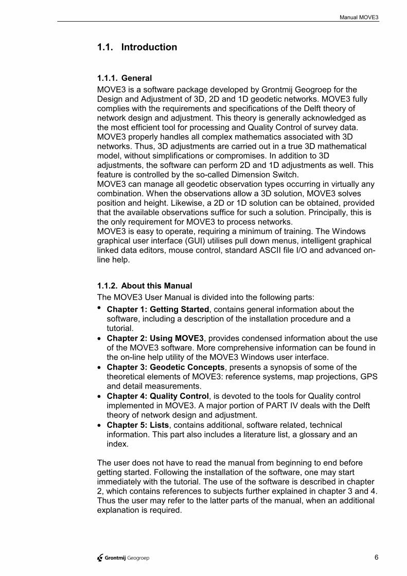
1.1.2. About this ManualThe MOVE3 User Manual is divided into the following parts:• Chapter 1: Getting Started, contains general information about the
software, including a description of the installation procedure and atutorial.
• Chapter 2: Using MOVE3, provides condensed information about the useof the MOVE3 software. More comprehensive information can be found inthe on-line help utility of the MOVE3 Windows user interface.
• Chapter 3: Geodetic Concepts, presents a synopsis of some of thetheoretical elements of MOVE3: reference systems, map projections, GPSand detail measurements.
• Chapter 4: Quality Control, is devoted to the tools for Quality controlimplemented in MOVE3. A major portion of PART IV deals with the Delfttheory of network design and adjustment.
• Chapter 5: Lists, contains additional, software related, technicalinformation. This part also includes a literature list, a glossary and anindex.
The user does not have to read the manual from beginning to end beforegetting started. Following the installation of the software, one may startimmediately with the tutorial. The use of the software is described in chapter2, which contains references to subjects further explained in chapter 3 and 4.Thus the user may refer to the latter parts of the manual, when an additionalexplanation is required.

Introduction Manual MOVE3
@ Grontmij Geogroep 7
1.1.3. MOVE3 SpecificationsMinimal system requirements:• Windows 95/98 or Windows NT version 4.0 or later;• PC, pentium processor 90 Mhz;• 8 Mb RAM memory;• monitor (800 x 600 resolution).
CapacityThe maximum network size is limited only by the available hardware.
ObservationsMOVE3 can handle both terrestrial and GPS observations:• Directions (up to 100 independent series per station);• Distances (up to 10 scale factors per network);• Zenith angles (up to 10 refraction coefficients per network);• Azimuths (up to 10 azimuth offsets per network);• Height differences;• Local coordinates;• GPS Baselines;• Observed GPS coordinates;• Geometrical relations:
• angle between 3 points (incl. perpendicular);• parallel lines (incl. mutual distance);• collinearity;• perpendicular lines;• distance from point to line;• chainage and offset.
Processing Modes3D, 2D and 1D geodetic networks can be processed in:• Design mode, free network;• Design mode, constrained network;• Adjustment mode, free network;• Adjustment mode, constrained network.
ProjectionsThe following projections are supported:General:• Transverse Mercator;• Lambert;• Stereographic;
Specific:• RD (The Netherlands);• Lambert 72 (Belgium);• Gauss Krüger (Germany);• Local (Stereographic);• BRSO;• Malaysian RSO.

Introduction Manual MOVE3
@ Grontmij Geogroep 8
ToolsMOVE3 includes separate tools such as fully automatic computation ofapproximate coordinates (COGO3), automatic loop detection and misclosuretesting (LOOPS3) and adjustment pre-analysis (PRERUN3).
General• Open file specifications (ASCII files);• Language support : English, Dutch;• Interfaces with GPS baseline processing packages (Ashtech, DSNP,
Leica, Sokkia, Spectra Precision, Topcon, Trimble and Zeiss);• Interfaces with digital levelling files from Leica, Topcon, Sokkia and Zeiss
digital levels;• Interface with De Min geoid model (The Netherlands);• Exporting DXF files;• On-line help facilities.
Manual MOVE3
@ Grontmij Geogroep 9
1.2. Installation
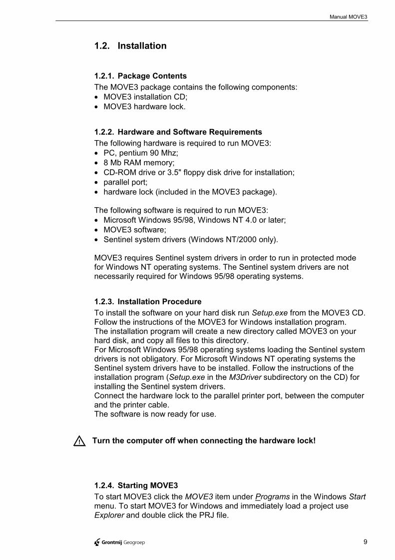
1.2.1. Package ContentsThe MOVE3 package contains the following components:• MOVE3 installation CD;• MOVE3 hardware lock.
1.2.2. Hardware and Software RequirementsThe following hardware is required to run MOVE3:• PC, pentium 90 Mhz;• 8 Mb RAM memory;• CD-ROM drive or 3.5" floppy disk drive for installation;• parallel port;• hardware lock (included in the MOVE3 package).
The following software is required to run MOVE3:• Microsoft Windows 95/98, Windows NT 4.0 or later;• MOVE3 software;• Sentinel system drivers (Windows NT/2000 only).
MOVE3 requires Sentinel system drivers in order to run in protected modefor Windows NT operating systems. The Sentinel system drivers are notnecessarily required for Windows 95/98 operating systems.
1.2.3. Installation ProcedureTo install the software on your hard disk run Setup.exe from the MOVE3 CD.Follow the instructions of the MOVE3 for Windows installation program.The installation program will create a new directory called MOVE3 on yourhard disk, and copy all files to this directory.For Microsoft Windows 95/98 operating systems loading the Sentinel systemdrivers is not obligatory. For Microsoft Windows NT operating systems theSentinel system drivers have to be installed. Follow the instructions of theinstallation program (Setup.exe in the M3Driver subdirectory on the CD) forinstalling the Sentinel system drivers.Connect the hardware lock to the parallel printer port, between the computerand the printer cable.The software is now ready for use.
! Turn the computer off when connecting the hardware lock!
1.2.4. Starting MOVE3To start MOVE3 click the MOVE3 item under Programs in the Windows Startmenu. To start MOVE3 for Windows and immediately load a project useExplorer and double click the PRJ file.

Manual MOVE3
@ Grontmij Geogroep 10
1.3. Tutorial
1.3.1. IntroductionIn this tutorial the following conventions are used:
Italics Italics represent text as it appears on screen. This format is also used for anythingyou must type literally.
Underline The hot key of the MOVE3 menu options is shown underlined, similar to theappearance on the screen.
In this tutorial a basic knowledge of Windows-based applications isassumed. For more information please refer to your Windows user manual.When you have properly installed the MOVE3 software according to theprevious instructions, there will be a number of demo files present in theM3SAMPLE directory. The demo files contain data of a small network,shaped as a braced quadrilateral, called 'Kamerik'. The network containsboth terrestrial and GPS observations: directions, distances, zenith angles,height differences and GPS baselines. This network should not be regardedas representative for the average survey project; it serves merely as ameans to illustrate the main MOVE3 features.
The following subjects will be demonstrated hereafter:• starting MOVE3;• handling a project;• controlling geometry and dimension;• editing;• adjustment in phases and testing;• saving a project and leaving MOVE3.
1.3.2. Starting and Using MOVE3 for WindowsTo start MOVE3 for Windows click the MOVE3 item under Programs.You are now in the MOVE3 Windows graphical user interface (GUI). Thisinterface can be used to create new projects, edit data, start computationsand view the results. The horizontal menu bar lists the names of theavailable drop down menus.
1.3.3. ProjectsYou are about to open the demo project Kamerik. In MOVE3 a project isdefined, as a group of files comprising all data needed to process a network.The project Kamerik consists of:
kamerik.prj project file with options and parameters
kamerik.tco terrestrial coordinate file
kamerik.gco GPS coordinate file
kamerik.obs observations file
Tutorial Manual MOVE3
@ Grontmij Geogroep 11
The PRJ file is the key file in the project because it contains the parameters,which control how the network is processed. For this reason projects areopened and saved by selecting the corresponding PRJ file.From the Project menu select Open.... A file selection box opens showing bydefault all PRJ files in the current directory. Select KAMERIK.PRJ from thesubdirectory M3SAMPLE. As a result the input files of this project are readas indicated by the message box. The Kamerik network appears on yourscreen.
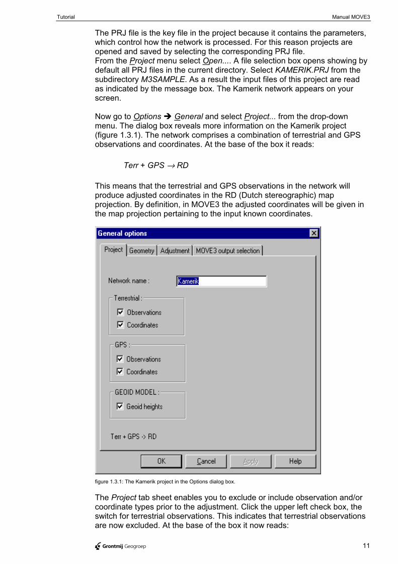
Now go to Options � General and select Project... from the drop-downmenu. The dialog box reveals more information on the Kamerik project(figure 1.3.1). The network comprises a combination of terrestrial and GPSobservations and coordinates. At the base of the box it reads:
Terr + GPS → RD
This means that the terrestrial and GPS observations in the network willproduce adjusted coordinates in the RD (Dutch stereographic) mapprojection. By definition, in MOVE3 the adjusted coordinates will be given inthe map projection pertaining to the input known coordinates.
figure 1.3.1: The Kamerik project in the Options dialog box.
The Project tab sheet enables you to exclude or include observation and/orcoordinate types prior to the adjustment. Click the upper left check box, theswitch for terrestrial observations. This indicates that terrestrial observationsare now excluded. At the base of the box it now reads:
Tutorial Manual MOVE3
@ Grontmij Geogroep 12
GPS → RD
Switch the terrestrial observations back on.
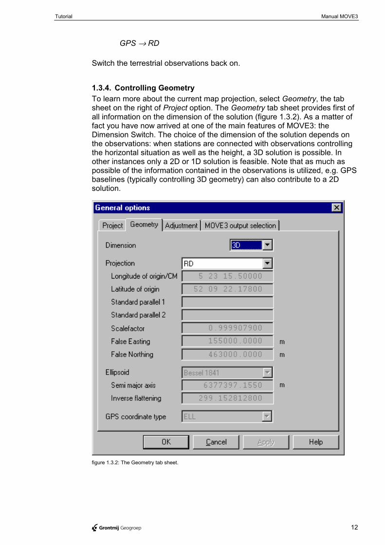
1.3.4. Controlling GeometryTo learn more about the current map projection, select Geometry, the tabsheet on the right of Project option. The Geometry tab sheet provides first ofall information on the dimension of the solution (figure 1.3.2). As a matter offact you have now arrived at one of the main features of MOVE3: theDimension Switch. The choice of the dimension of the solution depends onthe observations: when stations are connected with observations controllingthe horizontal situation as well as the height, a 3D solution is possible. Inother instances only a 2D or 1D solution is feasible. Note that as much aspossible of the information contained in the observations is utilized, e.g. GPSbaselines (typically controlling 3D geometry) can also contribute to a 2Dsolution.
figure 1.3.2: The Geometry tab sheet.
Tutorial Manual MOVE3
@ Grontmij Geogroep 13
Now move to the Projection drop-down list box, and have a look at the mapprojections supported by MOVE3. Some projections are completelypredefined, for others you must enter certain parameters, e.g. the centralmeridian in case of a UTM projection. In MOVE3 the ellipsoid is of vitalimportance. The ellipsoid is the reference surface in the adjustment. It isnecessary to specify an ellipsoid for every adjustment, even when you arenot using a map projection. Make sure the dimension is 3D and the mapprojection is RD and close the Options box by clicking the OK button.
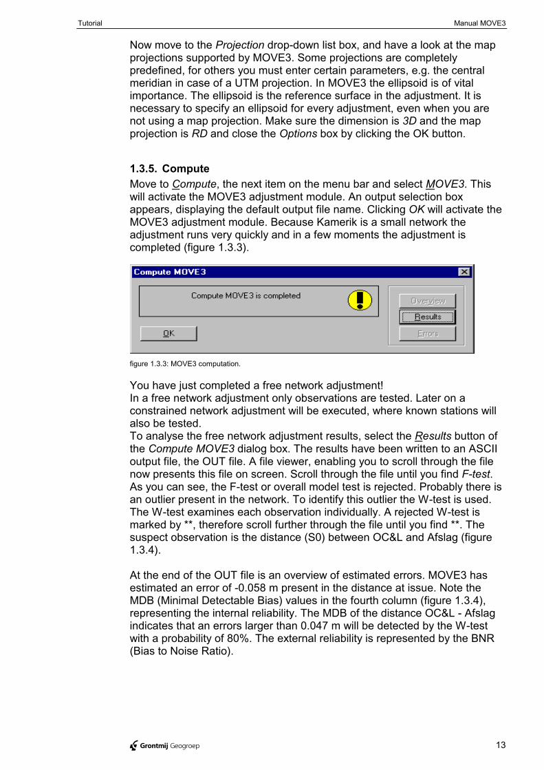
1.3.5. ComputeMove to Compute, the next item on the menu bar and select MOVE3. Thiswill activate the MOVE3 adjustment module. An output selection boxappears, displaying the default output file name. Clicking OK will activate theMOVE3 adjustment module. Because Kamerik is a small network theadjustment runs very quickly and in a few moments the adjustment iscompleted (figure 1.3.3).
figure 1.3.3: MOVE3 computation.
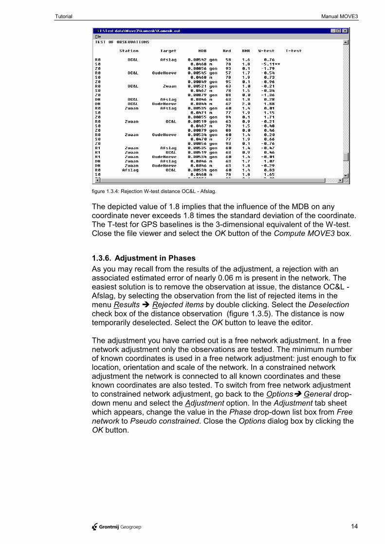
You have just completed a free network adjustment!In a free network adjustment only observations are tested. Later on aconstrained network adjustment will be executed, where known stations willalso be tested.To analyse the free network adjustment results, select the Results button ofthe Compute MOVE3 dialog box. The results have been written to an ASCIIoutput file, the OUT file. A file viewer, enabling you to scroll through the filenow presents this file on screen. Scroll through the file until you find F-test.As you can see, the F-test or overall model test is rejected. Probably there isan outlier present in the network. To identify this outlier the W-test is used.The W-test examines each observation individually. A rejected W-test ismarked by **, therefore scroll further through the file until you find **. Thesuspect observation is the distance (S0) between OC&L and Afslag (figure1.3.4).
At the end of the OUT file is an overview of estimated errors. MOVE3 hasestimated an error of -0.058 m present in the distance at issue. Note theMDB (Minimal Detectable Bias) values in the fourth column (figure 1.3.4),representing the internal reliability. The MDB of the distance OC&L - Afslagindicates that an errors larger than 0.047 m will be detected by the W-testwith a probability of 80%. The external reliability is represented by the BNR(Bias to Noise Ratio).
Tutorial Manual MOVE3
@ Grontmij Geogroep 14
figure 1.3.4: Rejection W-test distance OC&L - Afslag.
The depicted value of 1.8 implies that the influence of the MDB on anycoordinate never exceeds 1.8 times the standard deviation of the coordinate.The T-test for GPS baselines is the 3-dimensional equivalent of the W-test.Close the file viewer and select the OK button of the Compute MOVE3 box.
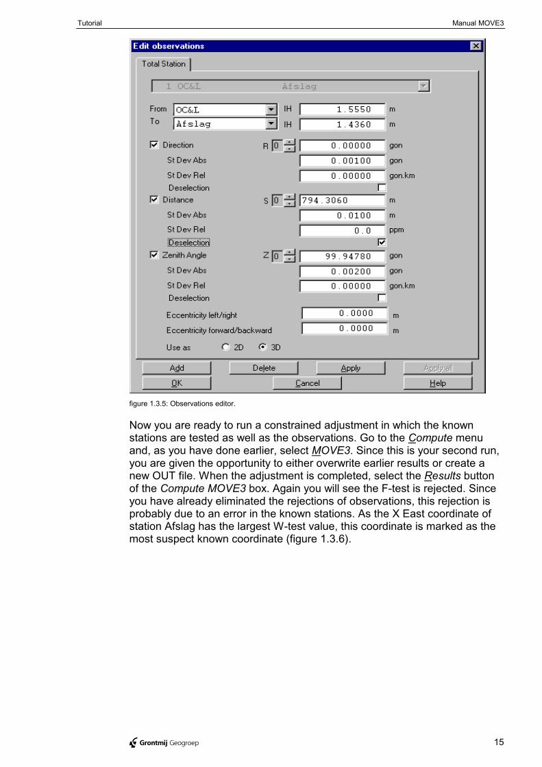
1.3.6. Adjustment in PhasesAs you may recall from the results of the adjustment, a rejection with anassociated estimated error of nearly 0.06 m is present in the network. Theeasiest solution is to remove the observation at issue, the distance OC&L -Afslag, by selecting the observation from the list of rejected items in themenu Results � Rejected items by double clicking. Select the Deselectioncheck box of the distance observation (figure 1.3.5). The distance is nowtemporarily deselected. Select the OK button to leave the editor.
The adjustment you have carried out is a free network adjustment. In a freenetwork adjustment only the observations are tested. The minimum numberof known coordinates is used in a free network adjustment: just enough to fixlocation, orientation and scale of the network. In a constrained networkadjustment the network is connected to all known coordinates and theseknown coordinates are also tested. To switch from free network adjustmentto constrained network adjustment, go back to the Options� General drop-down menu and select the Adjustment option. In the Adjustment tab sheetwhich appears, change the value in the Phase drop-down list box from Freenetwork to Pseudo constrained. Close the Options dialog box by clicking theOK button.
Tutorial Manual MOVE3
@ Grontmij Geogroep 15
figure 1.3.5: Observations editor.
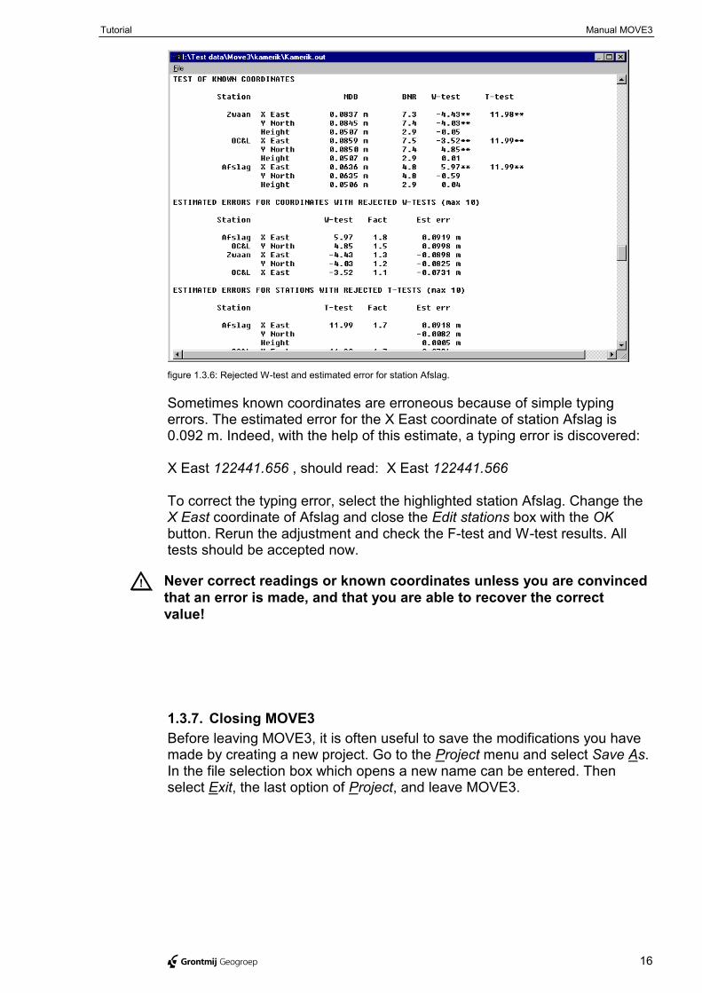
Now you are ready to run a constrained adjustment in which the knownstations are tested as well as the observations. Go to the Compute menuand, as you have done earlier, select MOVE3. Since this is your second run,you are given the opportunity to either overwrite earlier results or create anew OUT file. When the adjustment is completed, select the Results buttonof the Compute MOVE3 box. Again you will see the F-test is rejected. Sinceyou have already eliminated the rejections of observations, this rejection isprobably due to an error in the known stations. As the X East coordinate ofstation Afslag has the largest W-test value, this coordinate is marked as themost suspect known coordinate (figure 1.3.6).
Tutorial Manual MOVE3
@ Grontmij Geogroep 16
figure 1.3.6: Rejected W-test and estimated error for station Afslag.
Sometimes known coordinates are erroneous because of simple typingerrors. The estimated error for the X East coordinate of station Afslag is0.092 m. Indeed, with the help of this estimate, a typing error is discovered:
X East 122441.656 , should read: X East 122441.566
To correct the typing error, select the highlighted station Afslag. Change theX East coordinate of Afslag and close the Edit stations box with the OKbutton. Rerun the adjustment and check the F-test and W-test results. Alltests should be accepted now.
! Never correct readings or known coordinates unless you are convincedthat an error is made, and that you are able to recover the correctvalue!
1.3.7. Closing MOVE3Before leaving MOVE3, it is often useful to save the modifications you havemade by creating a new project. Go to the Project menu and select Save As.In the file selection box which opens a new name can be entered. Thenselect Exit, the last option of Project, and leave MOVE3.

Manual MOVE3
@ Grontmij Geogroep 17
2. Using MOVE3
Manual MOVE3
@ Grontmij Geogroep 18
2.1. IntroductionPart 2 of this manual provides the user with information about the use of theMOVE3 network adjustment software. The software consists of a Windowsuser interface and a number of computation modules. The Windows userinterface provides the user with full control over all options and parametersnecessary for the computation modules.The options and parameters are described in the on-line help utility of theMOVE3 Windows user interface. The option parameters are examined interms of defaults, possible values, and their effect on the software.In this part of the manual the MOVE3 model is discussed. A major part isdedicated to one of the main features of MOVE3: the Dimension Switch. Theuse of the Dimension Switch itself is rather straightforward. The choice ofdimension however, will have an effect on the handling of observation types.Therefore the chapter on the Dimension Switch is essential reading matter.
2.1.1. System OverviewAll tasks, which are performed by MOVE3, are initiated from the Windowsuser interface. Hence the user never has to leave the user interface duringan adjustment session in order to e.g. view or change the data. In generalthe data is managed, i.e. read, edited, displayed and saved, by the userinterface and processed, i.e. prepared, checked and adjusted, by the othercomputation modules.The software system comprises the following computation modules:• COGO3 to compute approximate coordinates;• GEOID3 to extract geoid heights from the De Min geoid model (The
Netherlands);• LOOPS3 to detect network loops and compute loop misclosures;• PRERUN3 to perform pre-adjustment analysis;• MOVE3 to perform design and adjustment computations.
Manual MOVE3
@ Grontmij Geogroep 19
2.2. MOVE3 Model
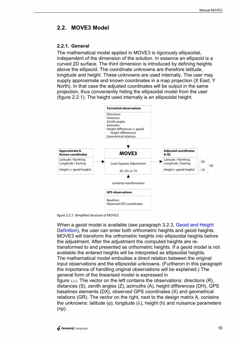
2.2.1. GeneralThe mathematical model applied in MOVE3 is rigorously ellipsoidal,independent of the dimension of the solution. In essence an ellipsoid is acurved 2D surface. The third dimension is introduced by defining heightsabove the ellipsoid. The coordinate unknowns are therefore latitude,longitude and height. These unknowns are used internally. The user maysupply approximate and known coordinates in a map projection (X East, YNorth). In that case the adjusted coordinates will be output in the sameprojection, thus conveniently hiding the ellipsoidal model from the user(figure 2.2.1). The height used internally is an ellipsoidal height.
Latitude / NorthingLongitude / Easting
Latitude / NorthingLongitude / Easting
Height (+ geoid height) Height (- geoid height)
Approximate &Known coordinates
Adjusted coordinates& QCMOVE3
Least Squares Adjustment
3D, 2D, or 1D
BaselinesObserved GPS coordinates
DirectionsDistancesZenith anglesAzimuthsHeight differences (+ geoid
height differences)Geometrical relations
Terrestrial observations
GPS observations
similarity transformation
2D
1D3D
figure 2.2.1: Simplified structure of MOVE3.
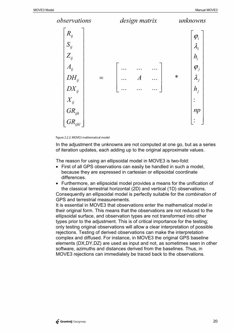
When a geoid model is available (see paragraph 3.2.3, Geoid and HeightDefinition), the user can enter both orthometric heights and geoid heights.MOVE3 will transform the orthometric heights into ellipsoidal heights beforethe adjustment. After the adjustment the computed heights are re-transformed to and presented as orthometric heights. If a geoid model is notavailable the entered heights will be interpreted as ellipsoidal heights.The mathematical model embodies a direct relation between the originalinput observations and the ellipsoidal unknowns. (Furtheron in this paragraphthe importance of handling original observations will be explained.) Thegeneral form of the linearised model is expressed infigure 2.2.2. The vector on the left contains the observations: directions (R),distances (S), zenith angles (Z), azimuths (A), height differences (DH), GPSbaselines elements (DX), observed GPS coordinates (X) and geometricalrelations (GR). The vector on the right, next to the design matrix A, containsthe unknowns: latitude (ϕ), longitude (λ), height (h) and nuisance parameters(np).
MOVE3 Model Manual MOVE3
@ Grontmij Geogroep 20
observations design matrix unknowns
RSZADHDXXGRGR
ij
ij
ij
ij
ij
ij
ij
ijk
ijkl
�
�
��������������
�
�
��������������
=�
�
���
�
�
���
�
�
�������������
�
�
�������������
... ... ...
... ...
... ... ...*
:
:
A
h
h
np
i
i
i
j
j
j
ϕλ
ϕλ
figure 2.2.2: MOVE3 mathematical model
In the adjustment the unknowns are not computed at one go, but as a seriesof iteration updates, each adding up to the original approximate values.
The reason for using an ellipsoidal model in MOVE3 is two-fold:• First of all GPS observations can easily be handled in such a model,
because they are expressed in cartesian or ellipsoidal coordinatedifferences.
• Furthermore, an ellipsoidal model provides a means for the unification ofthe classical terrestrial horizontal (2D) and vertical (1D) observations.
Consequently an ellipsoidal model is perfectly suitable for the combination ofGPS and terrestrial measurements.It is essential in MOVE3 that observations enter the mathematical model intheir original form. This means that the observations are not reduced to theellipsoidal surface, and observation types are not transformed into othertypes prior to the adjustment. This is of critical importance for the testing;only testing original observations will allow a clear interpretation of possiblerejections. Testing of derived observations can make the interpretationcomplex and diffused. For instance, in MOVE3 the original GPS baselineelements (DX,DY,DZ) are used as input and not, as sometimes seen in othersoftware, azimuths and distances derived from the baselines. Thus, inMOVE3 rejections can immediately be traced back to the observations.
MOVE3 Model Manual MOVE3
@ Grontmij Geogroep 21
Another advantage of working with an ellipsoidal model, with latitude andlongitude as coordinate unknowns, is that the map projection is neatly keptout of the adjustment. This advantage can be clarified if we look at thealternative, which is a map projection plane as reference surface in theadjustment. It then becomes necessary to account for the distortion, inherentto map projections, within the adjustment (see paragraph 3.3.1, Purposesand Methods of Projections). Usually these distortions are too complex forthe linearised mathematical model to handle. This makes the adjustmentusing a map projection plane only locally applicable for networks of limitedsize, whereas the mathematical model in MOVE3 imposes no limits on thesize of the network at all.To summarise the advantages of the ellipsoidal model in MOVE3, one couldsay that:• The ellipsoidal model is best suited for the combination of GPS and
terrestrial measurements.• The original observations are tested, and not observation derivatives. This
allows for a clear link between the testing and the observations.• The distortion due to the map projection is accounted for by applying map
projection formulas before the adjustment. This makes MOVE3 applicablefor networks of any size.
2.2.2. Observation TypesMOVE3 can handle the following observation types:• directions [R];• distances [S];• zenith angles [Z];• azimuths [A];• height differences [DH];• local coordinates [E], [N], [H];• GPS baselines [DX];• observed GPS coordinates [X];• 2D geometrical relations [GR]:
• angle between 3 points [AN];• perpendicular [PD];• collinearity (3 points on one line) [CL];• distance point-line [PL];
• parallel lines [PA], including mutual distance [LL];• perpendicular lines [AL];• chainage [CH] and offset [PL].
Directions.In MOVE3 directions are horizontal directions given in GON (centesimaldegrees), DEG (sexagesimal degrees) or DMS (degrees, minutes, seconds).A direction is represented by observation type R, followed by a digitspecifying the series, default R0. A maximum of 100 series per station isallowed.
MOVE3 Model Manual MOVE3
@ Grontmij Geogroep 22
Distances.In MOVE3 distances are regarded as horizontal or slope, depending on thedimension of the solution and on the availability of zenith angles (seeparagraph 2.2.3, Dimension Switch and Observation Type). Distances aregiven in meters. A distance is represented by observation type S, followed bya digit specifying the associated scale factor, default S0. A maximum of 10scale factors per network is allowed.
Zenith angles.In MOVE3 a zenith angle is given in GON (centesimal degrees), DEG(sexagesimal degrees) or DMS (degrees, minutes, seconds). A zenith angleis represented by observation type Z, followed by a digit specifying theassociated vertical refraction coefficient, default Z0. A maximum of 10refraction coefficients per network is allowed.
! The direction series (R0..R9) have no relationship with scale factors(S0..S9) and refraction coefficients (Z0..Z9). For example: a totalstation record can consist of R1, S0 and Z0.
Total station record.Directions, distances and zenith angles may be combined on oneobservation record; a so-called total station record. Other allowedcombinations are:• direction and distance;• direction and zenith angle;• distance and zenith angle.
The interpretation of these combinations depends on the dimension of thesolution and the dimension of the record (see paragraph 2.2.3, DimensionSwitch and Observation Type).
Azimuths.In MOVE3 an azimuth is a horizontal direction giving the angle between thenorth direction and the direction to a target. Azimuths are given in GON(centesimal degrees), DEG (sexagesimal degrees) or DMS (degrees,minutes, seconds). An azimuth is represented by observation type A,followed by a digit specifying the associated azimuth offset, default A0. Amaximum of 10 offsets per network is allowed.
Height differences.In MOVE3 height differences are given in meters. When a geoid model isavailable, the levelled (and/or trigonometric) height differences andorthometric heights are converted to ellipsoidal height differences andheights prior to the adjustment (see paragraph 3.2.3, Geoid and HeightDefinition). The heights presented after the adjustment are againorthometric. When a geoid model is not available, the known heights andheight differences are interpreted as ellipsoidal heights and heightdifferences. No conversion is applied in that case. A height difference isrepresented by observation type DH.
MOVE3 Model Manual MOVE3
@ Grontmij Geogroep 23
Local coordinates.A Local coordinate in MOVE3 is a coordinate set in the selected projection.The observation may consist of X East and Y North coordinates only, heightonly or a conbination of XY and height. The observation type is E for theEasting, N for the Northing and H for the height.
GPS baselines.In MOVE3 a GPS baseline is a 3D vector comprising three cartesiancoordinate differences in GPS. (In some receiver post processing software itis allowed to specify a reference systems different from WGS'84. In anycase, MOVE3 assumes baselines are given WGS'84.) GPS baselines aregiven in meters, and are represented by observation type DX.
Observed GPS coordinates.In MOVE3 an observed GPS coordinate is a 3D cartesian coordinate inWGS'84. They are useful for approximate determination of the seventransformation parameters between WGS'84 and the user defined localdatum. Observed GPS coordinates are given in meters, and arerepresented by observation type X.
Geometrical relations.The observation types related to more than two stations are captured underthe name geometrical relations. Following geometrical relations can be usedin MOVE3:Angle, an arbitrary horizontal angle between three points, expressed in GON(centesimal degrees), DEG (sexagesimal degrees) or DMS (degrees,minutes, seconds). An angle is represented by the observation type AN.Perpendicular, the perpendicular angle between 3 points (100 or 300 gon).MOVE3 will determine, based on the approximate coordinates which angle isapplicable. The standard deviation is given in GON, DEG or DMS and theobservation type for perpendicular is PD.Collinearity, the relation that 3 points are located on a straight line, thestandard deviation for collinearity is given in meters, the observation type isCL.Distance point - line, the perpendicular distance of a point to a line(consisting of two other points). The distance is given in meters and theobservation type is PL.Parallelism, two lines are parallel. The two lines each consist of two points.The standard deviation is given in GON, DEG or DMS and the observationtype for parallelism is PA.Distance between two parallel lines, between two parallel lines a distancecan be measured. The distance is given in meters and the observation typeis LL.Perpendicular lines, two lines a perpendicular to each other. MOVE3 willdetermine, based on the approximate coordinates which angle is applicable(100 or 300 gon). The standard deviation is given GON, DEG or DMS andthe observation type is AL.Chainage and offset, a combination of chainage, distance to the beginningof the measurement line, and the offset, the perpendicular distance to thisline, given in meters. The observation type for chainage is CH and for offsetPL. Chainage and offset can only be used as a combination of both.
MOVE3 Model Manual MOVE3
@ Grontmij Geogroep 24
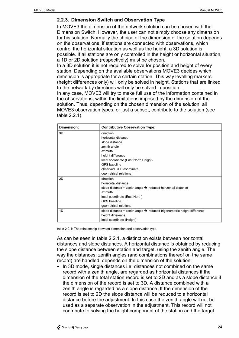
2.2.3. Dimension Switch and Observation TypeIn MOVE3 the dimension of the network solution can be chosen with theDimension Switch. However, the user can not simply choose any dimensionfor his solution. Normally the choice of the dimension of the solution dependson the observations: if stations are connected with observations, whichcontrol the horizontal situation as well as the height, a 3D solution ispossible. If all stations are only controlled in the height or horizontal situation,a 1D or 2D solution (respectively) must be chosen.In a 3D solution it is not required to solve for position and height of everystation. Depending on the available observations MOVE3 decides whichdimension is appropriate for a certain station. This way levelling markers(height differences only) will only be solved in height. Stations that are linkedto the network by directions will only be solved in position.In any case, MOVE3 will try to make full use of the information contained inthe observations, within the limitations imposed by the dimension of thesolution. Thus, depending on the chosen dimension of the solution, allMOVE3 observation types, or just a subset, contribute to the solution (seetable 2.2.1).
Dimension: Contributive Observation Type:3D direction
horizontal distanceslope distancezenith angleazimuthheight differencelocal coordinate (East North Height)GPS baselineobserved GPS coordinategeometrical relations
2D directionhorizontal distanceslope distance + zenith angle � reduced horizontal distanceazimuthlocal coordinate (East North)GPS baselinegeometrical relations
1D slope distance + zenith angle � reduced trigonometric height differenceheight differencelocal coordinate (Height)
table 2.2.1: The relationship between dimension and observation type.
As can be seen in table 2.2.1, a distinction exists between horizontaldistances and slope distances. A horizontal distance is obtained by reducingthe slope distance between station and target, using the zenith angle. Theway the distances, zenith angles (and combinations thereof on the samerecord) are handled, depends on the dimension of the solution:• In 3D mode, single distances i.e. distances not combined on the same
record with a zenith angle, are regarded as horizontal distances if thedimension of the total station record is set to 2D and as a slope distance ifthe dimension of the record is set to 3D. A distance combined with azenith angle is regarded as a slope distance. If the dimension of therecord is set to 2D the slope distance will be reduced to a horizontaldistance before the adjustment. In this case the zenith angle will not beused as a separate observation in the adjustment. This record will notcontribute to solving the height component of the station and the target.
MOVE3 Model Manual MOVE3
@ Grontmij Geogroep 25
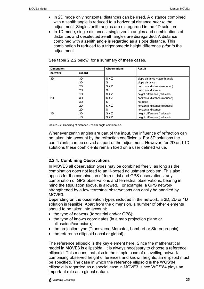
• In 2D mode only horizontal distances can be used. A distance combinedwith a zenith angle is reduced to a horizontal distance prior to theadjustment. Single zenith angles are disregarded in the 2D solution.
• In 1D mode, single distances, single zenith angles and combinations ofdistances and deselected zenith angles are disregarded. A distancecombined with a zenith angle is regarded as a slope distance. Thiscombination is reduced to a trigonometric height difference prior to theadjustment.
See table 2.2.2 below, for a summary of these cases.
Dimension Observations Resultnetwork record
3D 3D S + Z slope distance + zenith angle3D S slope distance2D S + Z horizontal distance (reduced)2D S horizontal distance1D S + Z height difference (reduced)
2D 3D S + Z horizontal distance (reduced)3D S not used2D S + Z horizontal distance (reduced)2D S horizontal distance
1D 3D1D
S + ZS + Z
height difference (reduced)height difference (reduced)
table 2.2.2: Handling of distance - zenith angle combination.
Whenever zenith angles are part of the input, the influence of refraction canbe taken into account by the refraction coefficients. For 3D solutions thecoefficients can be solved as part of the adjustment. However, for 2D and 1Dsolutions these coefficients remain fixed on a user defined value.
2.2.4. Combining ObservationsIn MOVE3 all observation types may be combined freely, as long as thecombination does not lead to an ill-posed adjustment problem. This alsoapplies for the combination of terrestrial and GPS observations; anycombination of GPS observations and terrestrial observations, bearing inmind the stipulation above, is allowed. For example, a GPS networkstrengthened by a few terrestrial observations can easily be handled byMOVE3.Depending on the observation types included in the network, a 3D, 2D or 1Dsolution is feasible. Apart from the dimension, a number of other elementsshould to be taken into account:• the type of network (terrestrial and/or GPS);• the type of known coordinates (in a map projection plane or
ellipsoidal/cartesian);• the projection type (Transverse Mercator, Lambert or Stereographic);• the reference ellipsoid (local or global).
The reference ellipsoid is the key element here. Since the mathematicalmodel in MOVE3 is ellipsoidal, it is always necessary to choose a referenceellipsoid. This means that also in the simple case of a levelling networkcomprising observed height differences and known heights, an ellipsoid mustbe specified. The case in which the reference ellipsoid is the WGS'84ellipsoid is regarded as a special case in MOVE3, since WGS'84 plays animportant role as a global datum.
MOVE3 Model Manual MOVE3
@ Grontmij Geogroep 26
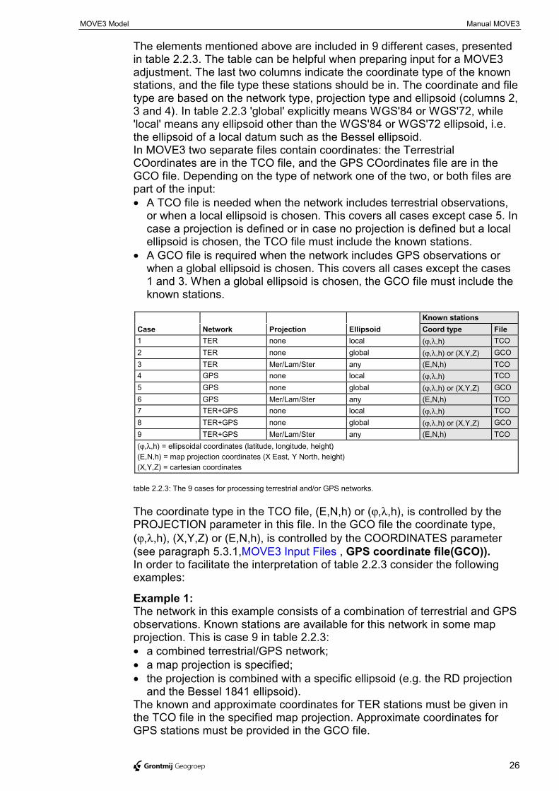
The elements mentioned above are included in 9 different cases, presentedin table 2.2.3. The table can be helpful when preparing input for a MOVE3adjustment. The last two columns indicate the coordinate type of the knownstations, and the file type these stations should be in. The coordinate and filetype are based on the network type, projection type and ellipsoid (columns 2,3 and 4). In table 2.2.3 'global' explicitly means WGS'84 or WGS'72, while'local' means any ellipsoid other than the WGS'84 or WGS'72 ellipsoid, i.e.the ellipsoid of a local datum such as the Bessel ellipsoid.In MOVE3 two separate files contain coordinates: the TerrestrialCOordinates are in the TCO file, and the GPS COordinates file are in theGCO file. Depending on the type of network one of the two, or both files arepart of the input:• A TCO file is needed when the network includes terrestrial observations,
or when a local ellipsoid is chosen. This covers all cases except case 5. Incase a projection is defined or in case no projection is defined but a localellipsoid is chosen, the TCO file must include the known stations.
• A GCO file is required when the network includes GPS observations orwhen a global ellipsoid is chosen. This covers all cases except the cases1 and 3. When a global ellipsoid is chosen, the GCO file must include theknown stations.
Known stationsCase Network Projection Ellipsoid Coord type File1 TER none local (ϕ,λ,h) TCO2 TER none global (ϕ,λ,h) or (X,Y,Z) GCO3 TER Mer/Lam/Ster any (E,N,h) TCO4 GPS none local (ϕ,λ,h) TCO5 GPS none global (ϕ,λ,h) or (X,Y,Z) GCO6 GPS Mer/Lam/Ster any (E,N,h) TCO7 TER+GPS none local (ϕ,λ,h) TCO8 TER+GPS none global (ϕ,λ,h) or (X,Y,Z) GCO9 TER+GPS Mer/Lam/Ster any (E,N,h) TCO(ϕ,λ,h) = ellipsoidal coordinates (latitude, longitude, height)(E,N,h) = map projection coordinates (X East, Y North, height)(X,Y,Z) = cartesian coordinates
table 2.2.3: The 9 cases for processing terrestrial and/or GPS networks.
The coordinate type in the TCO file, (E,N,h) or (ϕ,λ,h), is controlled by thePROJECTION parameter in this file. In the GCO file the coordinate type,(ϕ,λ,h), (X,Y,Z) or (E,N,h), is controlled by the COORDINATES parameter(see paragraph 5.3.1,MOVE3 Input Files , GPS coordinate file(GCO)).In order to facilitate the interpretation of table 2.2.3 consider the followingexamples:
Example 1:The network in this example consists of a combination of terrestrial and GPSobservations. Known stations are available for this network in some mapprojection. This is case 9 in table 2.2.3:• a combined terrestrial/GPS network;• a map projection is specified;• the projection is combined with a specific ellipsoid (e.g. the RD projection
and the Bessel 1841 ellipsoid).The known and approximate coordinates for TER stations must be given inthe TCO file in the specified map projection. Approximate coordinates forGPS stations must be provided in the GCO file.
MOVE3 Model Manual MOVE3
@ Grontmij Geogroep 27
Example 2:A simple 1D levelling network has to be adjusted. In order to link the networkto the reference ellipsoid, all stations must be given in 3D (approximate)coordinates. This is a consequence of the ellipsoidal model used in MOVE3.Hence, for a levelling network it is necessary to enter known heights andapproximate coordinates as (X East, Y North) or as (latitude, longitude).Presuming that the necessary approximate coordinates are scaled from atopographic map in some map projection case 3 in table 2.2.3 applies:• the network is terrestrial;• a map projection is specified;• the projection is combined with a specific ellipsoid (e.g. the RD projection
and the Bessel 1841 ellipsoid).The known and approximate coordinates must be given in the TCO file in thespecified map projection. A GCO file is not necessary.
Example 3:Consider the case of the free network adjustment of a GPS network. At thisstage the main concern is the correctness of the GPS observations, ratherthan the computation of the final adjusted coordinates. Therefore a mapprojection is not yet specified. The reference ellipsoid is then by definition theGPS reference ellipsoid WGS'84. This is case 5 in table 2.2.3:• a GPS network;• projection is none;• the reference ellipsoid is WGS'84.The known and approximate coordinates must be given in the GCO file. ATCO file is not necessary. Note that this example is valid for both 3D and 2D.
Although a variety of cases may occur, it is most likely in practice that theuser has known stations in some map projection at his disposal. Then, bydefinition, the known stations must be given in the TCO file. In case thenetwork includes GPS observations, approximate coordinates for the GPSstations must be given in the GCO file. Thus, the ellipsoidal model iscompletely concealed, and the user's only concern is the selection of theproper map projection and ellipsoid.
2.2.5. More information...More information about using the MOVE3 network adjustment software canbe found in the on-line help utility of the MOVE3 Windows user interface.To request Help, use one of the following methods:• From the Help menu, choose a Help command;• Press F1;• Choose the Help button available in the dialog box. This method gives you
quick access to specific information about the dialog box.
Manual MOVE3
@ Grontmij Geogroep 28
3. Geodetic Concepts
Manual MOVE3
@ Grontmij Geogroep 29
3.1. IntroductionThis part of the manual introduces the user to some of the theoreticalfundamentals of MOVE3. It is presumed that the user possesses some basicknowledge of surveying and adjustment computations. A completepresentation of all theoretical aspects is beyond the scope of this manual.The reader is referred to the literature list in paragraph 5.2, Literature List.
The mathematical model in MOVE3 is rigorously ellipsoidal. The coordinateunknowns are latitude, longitude and height. Consequently it is necessary toselect an ellipsoid as a reference system in the adjustment. In addition, inmany cases a map projection is required to relate the input Easting andNorthing to the internal ellipsoidal unknowns. Therefore, the paragraphs 3.2and 3.3 deal with reference systems and map projections. Another reasonfor discussing reference systems is the vital role of the World GeodeticSystem 1984 (WGS'84) in GPS positioning.
Paragraph 3.4 is dedicated to GPS. GPS is now an important measurementtool in many surveys. Hence a separate chapter of this manual is dedicatedto this subject. Of course this chapter will mainly focus on those aspects ofGPS which relate to MOVE3, namely relative positioning using phasemeasurements. Special attention will be paid to GPS in control networks.GPS allows for a different approach, especially when designing networks, ascompared to the classical approach with terrestrial observations. Last but notleast, the combination of GPS and terrestrial networks is discussed.
Paragraph 3.5, Detail Measurements treats the processing of detailmeasurements in the adjustment. Specific features as geometric relations,idealisation precision and offset measurements are explained.
Manual MOVE3
@ Grontmij Geogroep 30
3.2. Reference SystemsThe mathematical model in MOVE3 is rigorously ellipsoidal. This means thatMOVE3 internally uses ellipsoidal coordinates. Consequently the user has toselect an ellipsoid as reference surface in the adjustment. Therefore thischapter deals with reference systems in general, and the vital role of theWorld Geodetic System 1984 (WGS'84) in GPS positioning in particular.
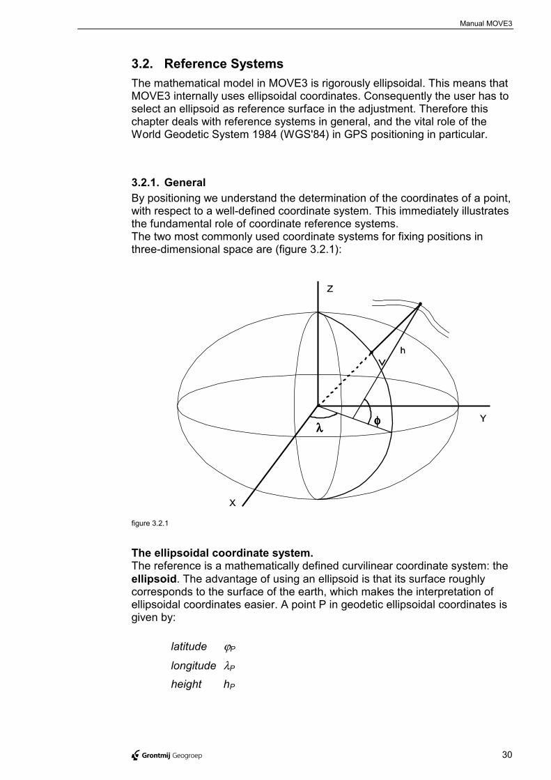
3.2.1. GeneralBy positioning we understand the determination of the coordinates of a point,with respect to a well-defined coordinate system. This immediately illustratesthe fundamental role of coordinate reference systems.The two most commonly used coordinate systems for fixing positions inthree-dimensional space are (figure 3.2.1):
φφφφλλλλ
figure 3.2.1
The ellipsoidal coordinate system.The reference is a mathematically defined curvilinear coordinate system: theellipsoid. The advantage of using an ellipsoid is that its surface roughlycorresponds to the surface of the earth, which makes the interpretation ofellipsoidal coordinates easier. A point P in geodetic ellipsoidal coordinates isgiven by:
latitude ϕP
longitude λP
height hP
Reference Systems Manual MOVE3
@ Grontmij Geogroep 31
The cartesian coordinate system.A point P in such a system is fixed by means of three distances to threeperpendicular axes X, Y and Z. The axes usually define a right-handedsystem. The XY plane is in the equatorial plane. The positive X-axis is in thedirection of the Greenwich meridian. The positive Z-axis, perpendicular to theXY plane points towards the North Pole. The coordinates of a point P aregiven as: Xp, Yp, Zp. A cartesian system is very suited for representation ofrelative positions, such as GPS baselines.
There is a direct relationship between the two coordinate systems. Hence,ellipsoidal coordinates can easily be transformed into cartesian coordinatesand vice versa.The ellipsoid itself is defined by its semi major axis a and semi minor axis b,or by its semi major axis and flattening f. There is a simple relationshipbetween the axes and the flattening:
f = (a - b) / a
The positioning of the ellipsoid requires six more parameters to eliminate thesix degrees of freedom, i.e. the six ways (three translations, three rotations)in which the ellipsoid can move relative to the earth. The task ofappropriately positioning a reference ellipsoid is known as the establishmentof a datum.In classical geodesy the reference ellipsoid is used as a horizontal datumonly. Heights are given with respect to mean sea level or, more precisely,with respect to the geoid. In this context the geoid serves as a vertical datum(see paragraph 3.2.3, Geoid and Height Definition).
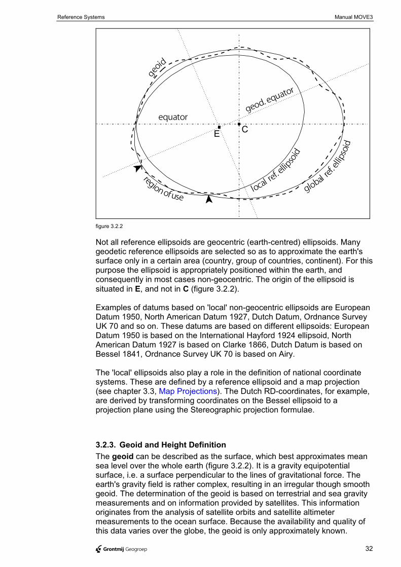
3.2.2. Global and Local SystemsA distinction can be made between global and local reference systems(figure 3.2.2). The GPS reference system WGS'84 for example, is a globalreference system. Its origin is supposed to coincide with the earth's centre ofgravity C, and its Z-axis is supposed to coincide with the earth's rotationalaxis. WGS'84 is the latest in a series of earth-centred, earth-fixed (ECEF)coordinate systems (WGS'60, WGS'66, WGS'72). Each of these systems isbased on updated information, and therefore successively more accurate.The general importance of WGS'84 is that it provides a means for relatingpositions in various local reference systems.
Reference Systems Manual MOVE3
@ Grontmij Geogroep 32
region of use
equator
local ref. ellip
soid
global re
f. ellip
soid
CE
geoid
geod. equator
figure 3.2.2
Not all reference ellipsoids are geocentric (earth-centred) ellipsoids. Manygeodetic reference ellipsoids are selected so as to approximate the earth'ssurface only in a certain area (country, group of countries, continent). For thispurpose the ellipsoid is appropriately positioned within the earth, andconsequently in most cases non-geocentric. The origin of the ellipsoid issituated in E, and not in C (figure 3.2.2).
Examples of datums based on 'local' non-geocentric ellipsoids are EuropeanDatum 1950, North American Datum 1927, Dutch Datum, Ordnance SurveyUK 70 and so on. These datums are based on different ellipsoids: EuropeanDatum 1950 is based on the International Hayford 1924 ellipsoid, NorthAmerican Datum 1927 is based on Clarke 1866, Dutch Datum is based onBessel 1841, Ordnance Survey UK 70 is based on Airy.
The 'local' ellipsoids also play a role in the definition of national coordinatesystems. These are defined by a reference ellipsoid and a map projection(see chapter 3.3, Map Projections). The Dutch RD-coordinates, for example,are derived by transforming coordinates on the Bessel ellipsoid to aprojection plane using the Stereographic projection formulae.
3.2.3. Geoid and Height DefinitionThe geoid can be described as the surface, which best approximates meansea level over the whole earth (figure 3.2.2). It is a gravity equipotentialsurface, i.e. a surface perpendicular to the lines of gravitational force. Theearth's gravity field is rather complex, resulting in an irregular though smoothgeoid. The determination of the geoid is based on terrestrial and sea gravitymeasurements and on information provided by satellites. This informationoriginates from the analysis of satellite orbits and satellite altimetermeasurements to the ocean surface. Because the availability and quality ofthis data varies over the globe, the geoid is only approximately known.
Reference Systems Manual MOVE3
@ Grontmij Geogroep 33
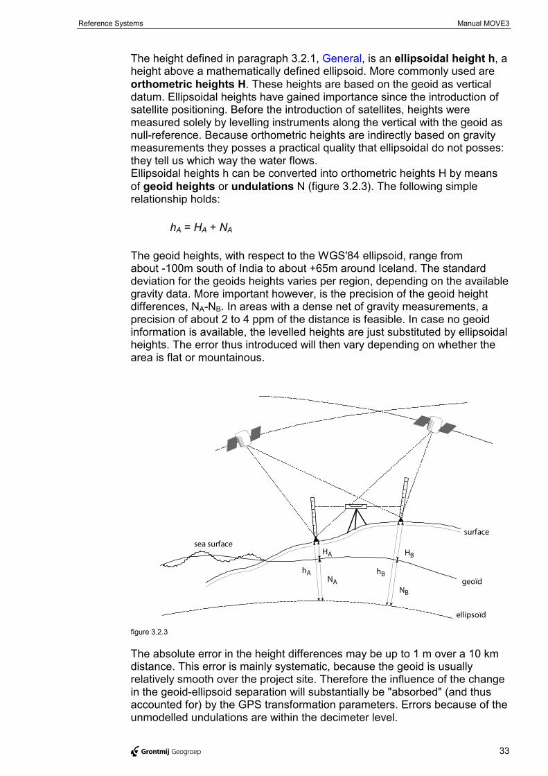
The height defined in paragraph 3.2.1, General, is an ellipsoidal height h, aheight above a mathematically defined ellipsoid. More commonly used areorthometric heights H. These heights are based on the geoid as verticaldatum. Ellipsoidal heights have gained importance since the introduction ofsatellite positioning. Before the introduction of satellites, heights weremeasured solely by levelling instruments along the vertical with the geoid asnull-reference. Because orthometric heights are indirectly based on gravitymeasurements they posses a practical quality that ellipsoidal do not posses:they tell us which way the water flows.Ellipsoidal heights h can be converted into orthometric heights H by meansof geoid heights or undulations N (figure 3.2.3). The following simplerelationship holds:
hA = HA + NA
The geoid heights, with respect to the WGS'84 ellipsoid, range fromabout -100m south of India to about +65m around Iceland. The standarddeviation for the geoids heights varies per region, depending on the availablegravity data. More important however, is the precision of the geoid heightdifferences, NA-NB. In areas with a dense net of gravity measurements, aprecision of about 2 to 4 ppm of the distance is feasible. In case no geoidinformation is available, the levelled heights are just substituted by ellipsoidalheights. The error thus introduced will then vary depending on whether thearea is flat or mountainous.
surface
geoïd
ellipsoïd
NB
HB
sea surface
NA
HA
hA hB
figure 3.2.3
The absolute error in the height differences may be up to 1 m over a 10 kmdistance. This error is mainly systematic, because the geoid is usuallyrelatively smooth over the project site. Therefore the influence of the changein the geoid-ellipsoid separation will substantially be "absorbed" (and thusaccounted for) by the GPS transformation parameters. Errors because of theunmodelled undulations are within the decimeter level.
Reference Systems Manual MOVE3
@ Grontmij Geogroep 34
The correct procedure, necessary for critical applications, is to convertorthometric heights and height differences into ellipsoidal heights and heightdifferences before the adjustment, using the available geoid heights. Afterthe adjustment the computed ellipsoidal heights are vice versa converted toorthometric heights.
3.2.4. Datum TransformationsGPS is indeed a global positioning system and is consequently based on aglobal datum. Characteristic for such a global or world datum is (seeparagraph 3.2.2, Global and Local Systems):• its origin is supposed to coincide with the earth's centre of mass;• its Z-axis is supposed to coincide with the earth's rotational axis.
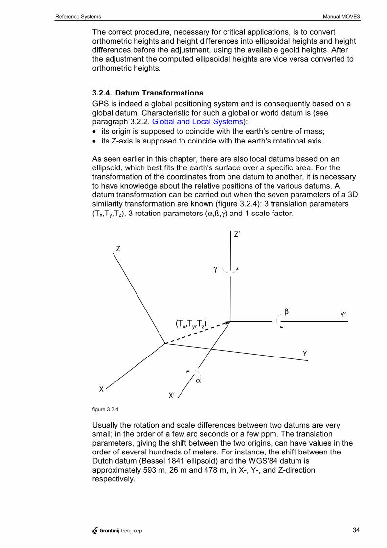
As seen earlier in this chapter, there are also local datums based on anellipsoid, which best fits the earth's surface over a specific area. For thetransformation of the coordinates from one datum to another, it is necessaryto have knowledge about the relative positions of the various datums. Adatum transformation can be carried out when the seven parameters of a 3Dsimilarity transformation are known (figure 3.2.4): 3 translation parameters(Tx,Ty,Tz), 3 rotation parameters (α,ß,γ) and 1 scale factor.
α
β
γ
(Tx,Ty,Tz)
Z’
Z
Y’
Y
X’X
figure 3.2.4
Usually the rotation and scale differences between two datums are verysmall; in the order of a few arc seconds or a few ppm. The translationparameters, giving the shift between the two origins, can have values in theorder of several hundreds of meters. For instance, the shift between theDutch datum (Bessel 1841 ellipsoid) and the WGS'84 datum isapproximately 593 m, 26 m and 478 m, in X-, Y-, and Z-directionrespectively.
Reference Systems Manual MOVE3
@ Grontmij Geogroep 35
When GPS observations are to be included in a local datum, in which e.g.the known stations are given, a transformation is necessary. For GPSbaselines, the translation between WGS'84 and the local datum need not besolved. Thus in the adjustment only 4 transformation parameters remain. InMOVE3 the 4 transformation parameters are solved as part of theadjustment. The user therefore does not have to enter these parameters. Asa consequence these parameters only have a local significance, andcannot be presumed valid for areas beyond the extent of the pertainingnetwork.Besides solving the transformation parameters it is also possible to keep thetransformation parameters fixed or weighted fixed.
! It is possible to solve for all 7-transformation parameters whenobserved GPS coordinates are included. Observed GPS coordinatesare a specific observation type in MOVE3 (see paragraph 2.2.2,Observation Types).
Manual MOVE3
@ Grontmij Geogroep 36
3.3. Map ProjectionsAfter a short general introduction, this chapter describes the most commonlyused map projections: the Transverse Mercator, the Lambert and theStereographic projection. Map projections are applied in MOVE3 to relate theentered X East and Y North coordinates to the internally used ellipsoidalcoordinates.
3.3.1. Purposes and Methods of ProjectionsIn surveying it is often more convenient to work with rectangular coordinateson a plane, than with ellipsoidal coordinates on a curved surface. Mapprojections (Fmp) are used to transform the ellipsoidal latitude and longitudeinto rectangular X East and Y North, and vice versa:
latitudelongitude
Fmp X EastY North
ϕλ���
→���
X EastY North
Fmp latitudelongitude
���
−
→���
1ϕ
λ
! The orientation of the planar coordinate system is often a source ofconfusion in map projections. In some countries, for instance inGermany, the positive X-axis points towards the north, while the positiveY-axis points toward the east. In other countries, for instance in theNetherlands, the situation is reversed. To avoid confusion, the X- and Y-coordinates are often referred to as Easting and Northing.
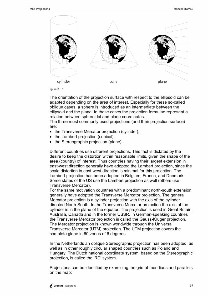
The representation of the curved ellipsoidal surface of the earth on a planewill inevitably result in a distortion of geometric elements. With respect to thisdistortion, map projections are usually subdivided in conformal, equidistantand equivalent projections. Conformal projections preserve the angle of anytwo curves on the ellipsoidal surface. Because of this property, onlyconformal projections are employed for geodetic purposes. Equidistant(equality of distances) and equivalent (equality of areas) projections aresometimes used in other disciplines, such as cartography.Another subdivision of map projections is based on the projection surface.Projections can then be subdivided into cylindrical, conical and plane,depending on whether the projection surface is a cylinder, a cone or a plane(figure 3.3.1).
Map Projections Manual MOVE3
@ Grontmij Geogroep 37
cylinder cone plane
figure 3.3.1
The orientation of the projection surface with respect to the ellipsoid can beadapted depending on the area of interest. Especially for these so-calledoblique cases, a sphere is introduced as an intermediate between theellipsoid and the plane. In these cases the projection formulae represent arelation between spheroidal and plane coordinates.The three most commonly used projections (and their projection surface)are:• the Transverse Mercator projection (cylinder);• the Lambert projection (conical);• the Stereographic projection (plane).
Different countries use different projections. This fact is dictated by thedesire to keep the distortion within reasonable limits, given the shape of thearea (country) of interest. Thus countries having their largest extension ineast-west direction generally have adopted the Lambert projection, since thescale distortion in east-west direction is minimal for this projection. TheLambert projection has been adopted in Belgium, France, and Denmark.Some states of the US use the Lambert projection as well (others useTransverse Mercator).For the same motivation countries with a predominant north-south extensiongenerally have adopted the Transverse Mercator projection. The generalMercator projection is a cylinder projection with the axis of the cylinderdirected North-South. In the Transverse Mercator projection the axis of thecylinder is in the plane of the equator. The projection is used in Great Britain,Australia, Canada and in the former USSR. In German-speaking countriesthe Transverse Mercator projection is called the Gauss-Krüger projection.The Mercator projection is known worldwide through the UniversalTransverse Mercator (UTM) projection. The UTM projection covers thecomplete globe in 60 zones of 6 degrees.
In the Netherlands an oblique Stereographic projection has been adopted, aswell as in other roughly circular shaped countries such as Poland andHungary. The Dutch national coordinate system, based on the Stereographicprojection, is called the 'RD' system.
Projections can be identified by examining the grid of meridians and parallelson the map:
Map Projections Manual MOVE3
@ Grontmij Geogroep 38
• In the Transverse Mercator projection the earth's equator and the centralmeridian, the tangent cylinder-ellipsoid, are projected as straight lines.Other meridians and parallels are projected as complex curves.
• The Lambert projection pictures parallels as unequally spaced arcs ofconcentric circles. Meridians are projected as equally spaced radii of thesame circles.
• The polar Stereographic projection pictures parallels as concentric circles,and meridians as straight lines radiating at true angles from the polarcentre of projection. The oblique alternative of this projection pictures allparallels and meridians as circles. Exceptions are the meridian oflongitude of origin, and the parallel opposite in sign to the parallel oflatitude of origin. The latter two are shown as straight lines.
Projections are defined by a number of parameters. The interpretation ofthese parameters may differ for the various projections. The parameters arereviewed in the next paragraphs.
3.3.2. The Transverse Mercator ProjectionThe Transverse Mercator projection is based on the following parameters:
Central Meridian (CM): Normally the meridian running through the centre of the area of interest,defining together with the latitude of origin the origin of the plane coordinatesystem. There is no scale distortion along the central meridian.
Longitude of Origin: See Central Meridian.
Latitude of Origin: Normally the parallel running through the centre of the area of interest,defining together with the central meridian the origin of the plane coordinatesystem.
Scale Factor: The scale factor is constant along the central meridian. The value assignedto the scale factor along this line is often slightly smaller than 1, so that theoverall scale of the map is more neatly correct.
False Easting: For some projections a False Easting is introduced to prevent negativecoordinates. A False Easting is simply a large positive value that is added tothe original Easting. In some cases the False Easting is assigned a specificvalue, making Eastings immediately distinguishable from Northings.
False Northing: For some projections a False Northing is introduced to prevent negativecoordinates. A False Northing is simply a large positive value that is addedto the original Northing. In some cases the False Northing is assigned aspecific value, making Northings immediately distinguishable from Eastings.
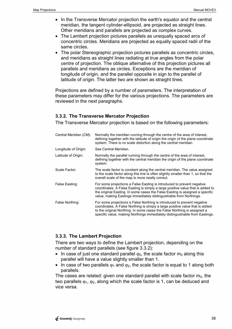
3.3.3. The Lambert ProjectionThere are two ways to define the Lambert projection, depending on thenumber of standard parallels (see figure 3.3.2):• In case of just one standard parallel ϕ0, the scale factor m0 along this
parallel will have a value slightly smaller than 1.• In case of two parallels ϕ1 and ϕ2, the scale factor is equal to 1 along both
parallels.The cases are related: given one standard parallel with scale factor m0, thetwo parallels ϕ1, ϕ2, along which the scale factor is 1, can be deduced andvice versa.
Map Projections Manual MOVE3
@ Grontmij Geogroep 39
m=1
m=1
m=1
m=1
mer
idia
n
m>1
m0
m<1
ϕ 1 ϕ 0 ϕ 2
m<1
figure 3.3.2
The Lambert projection is based on the following parameters:
Standard Parallel(s): Two standard parallels represent the intersecting circles of the cone and theellipsoid. A single standard parallel is usually not an intersecting circle, butrepresents a circle in between the two circles that intersect the cone.
Longitude of Origin: Normally the meridian running through the centre of the area of interest,defining together with the latitude of origin the origin of the plane coordinatesystem.
Latitude of Origin: Normally the parallel running through the centre of the area of interest,defining together with the longitude of origin the origin of the plane coordinatesystem.
Scale Factor: Sometimes a scale factor along the single standard parallel is introduced witha value slightly smaller than 1, so that the overall scale of the map is moreneatly correct.
False Easting: For some projections a False Easting is introduced to prevent negativecoordinates. A False Easting is simply a large positive value that is added tothe original Easting. In some cases the False Easting is assigned a specificvalue, making Eastings immediately distinguishable from Northings.
False Northing: For some projections a False Northing is introduced to prevent negativecoordinates. A False Northing is simply a large positive value that is added tothe original Northing. In some cases the False Northing is assigned a specificvalue, making Northings immediately distinguishable from Eastings.
3.3.4. The Stereographic ProjectionThe Stereographic projection is based on the following parameters:
Longitude of Origin: Longitude of the central point (the tangent point of ellipsoid and plane) of theprojection, usually in the centre of the area of interest.
Latitude of Origin: Latitude of the central point of the projection, usually in the centre of the areaof interest.
Scale Factor: The scale factor at the central point of the projection, as defined by thelatitude and longitude of origin. The value assigned to the scale factor at thispoint is often slightly smaller than 1, so that the overall scale of the map ismore neatly correct.
Map Projections Manual MOVE3
@ Grontmij Geogroep 40
False Easting: For some projections a False Easting is introduced to prevent negativecoordinates. A False Easting is simply a large positive value that is added tothe original Easting. In some cases the False Easting is assigned a specificvalue, making Eastings immediately distinguishable from Northings.
False Northing: For some projections a False Northing is introduced to prevent negativecoordinates. A False Northing is simply a large positive value that is added tothe original Northing. In some cases the False Northing is assigned a specificvalue, making Northings immediately distinguishable from Eastings.
3.3.5. The Local (Stereographic) ProjectionThe Local (Stereographic) projection is useful when the network coordinatesare given in your own local coordinate system. MOVE3 uses a stereographicprojection with the following default values for the parameters:
Longitude of Origin: 0°Latitude of Origin: 0°Scale Factor: 1.0False Easting: 0 mFalse Northing: 0 m
! The user is free to change these values.
Manual MOVE3
@ Grontmij Geogroep 41
3.4. GPSGPS is rapidly becoming the major measurement tool in many surveys.Therefore in the next few paragraphs the aspects of GPS which relate toMOVE3 are highlighted. Special attention will be paid to GPS in controlnetworks. GPS allows for a different approach, especially in designing thesenetworks, as compared to the classical approach with terrestrialobservations. In addition, the final paragraph discusses the combination ofGPS and terrestrial networks.
3.4.1. GeneralGPS can be used for various different purposes, from real time navigation tohigh precision relative positioning. In the latter case GPS has a number ofadvantages over the traditional land surveying methods:• the line of sight between station and target is no longer a requirement;• GPS observations (baselines) can span large distances;• observations have a high precision;• the measurement process is quick and efficient.The processing of GPS observations can be divided into two steps. In thefirst step the “raw” GPS observations, stored in the GPS receiver, areprocessed to get WGS’84 coordinates or WGS’84 coordinate differences(baselines). The processing is usually done with GPS post-processingsoftware supplied by the GPS receiver manufacturer. The GPS baselines arethe input for the second step, the MOVE3 adjustment. GPS is a globalsystem therefore GPS observations are expressed in the world-wideWGS’84 system (World Geodetic System 1984). To get local coordinatesfrom GPS observations a transformation is required (see paragraph 3.2.4,Datum Transformations).
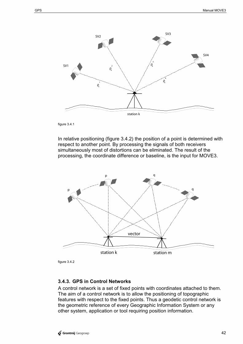
3.4.2. GPS ObservationsIn GPS positioning a distinction can be made between absolute and relativepositioning:• By absolute positioning (figure 3.4.1) we understand the determination of
the absolute coordinates of a point on land, at sea or in space with respectto a well-defined coordinate system, e.g. WGS'84. A major disadvantageof absolute positioning is the distortion of GPS signals by the controllers ofthe GPS system (Selective Availability) and distortion by atmosphericconditions. These effects influence the computed receiver's position.Therefore accurate absolute positioning is not possible with thistechnique. Accuracy can be improved by relative measurements (DGPS).
GPS Manual MOVE3
@ Grontmij Geogroep 42
station k
ρ1
k
ρ2
k
ρ3
k
ρ4
k
SV1
SV2SV3
SV4
figure 3.4.1
In relative positioning (figure 3.4.2) the position of a point is determined withrespect to another point. By processing the signals of both receiverssimultaneously most of distortions can be eliminated. The result of theprocessing, the coordinate difference or baseline, is the input for MOVE3.
station k station m
vector
p
p q
q
figure 3.4.2
3.4.3. GPS in Control NetworksA control network is a set of fixed points with coordinates attached to them.The aim of a control network is to allow the positioning of topographicfeatures with respect to the fixed points. Thus a geodetic control network isthe geometric reference of every Geographic Information System or anyother system, application or tool requiring position information.
GPS Manual MOVE3
@ Grontmij Geogroep 43
In point of fact, a GPS baseline is just one in the list of observation typesincluding directions, distances, zenith angles, azimuths and heightdifferences (see paragraph 2.2.2, Observation Types). However, GPSpossesses some features, which require a different approach when usingGPS in control networks:• The line of sight between adjacent network stations is no longer a
necessity. This, added to the fact that there is practically no limit to thedistance between receivers, provides the surveyor with an enormousamount of freedom when designing a network.
• GPS is a 3D-measurement technique. The strictly applied, though artificialdistinction between horizontal networks and height networks no longerholds.
• A characteristic of GPS is that all coordinates and coordinate differencesare given in the same unique world-wide reference system. This presentsa problem when GPS observations are linked to existing known stationsgiven in some local coordinate system. In such cases the parameters of asimilarity transformation have to be solved (see paragraph 3.2.4, DatumTransformations).
3.4.4. GPS stochastic modelAs a result of the GPS baseline processing besides the coordinatedifferences also a 3x3-variance matrix for the coordinates is computed (seeparagraph 4.2.3, Stochastic Model). This variance matrix can be used inMOVE3 for the precision of the baseline. In most cases however thecomputed standard deviations are too optimistic. This may cause rejectionsin all of the baselines. MOVE3 contains two tools to solve this problem. Thefirst is to scale the standard deviations of the baselines. A second possibilityis to use an absolute and relative standard deviation per baseline. Therelative part is usually expressed in ppm (parts per million of the baselinelength). In this case the correlation between the components of the baselineis ignored.
3.4.5. GPS and HeightsHeight differences measured with GPS are always ellipsoidal heightdifferences. To convert ellipsoidal height differences to orthometric heightdifferences a correction for the geoid needs to be applied (see paragraph3.2.3, Geoid and Height Definition). The precision of the height differences isusually rather limited, thus influencing the total precision of GPS heightdetermination.Even when the geoid is not taken into consideration, GPS cannot competewith levelling.
Manual MOVE3
@ Grontmij Geogroep 44
3.5. Detail Measurements
The target of detail measurements is to establish the mutual position ofobject in the field. Strictly spoken the detail measurements do not differ fromcontrol measurements, but a number of characteristics is specific for detailmeasurements. Detail networks usually contain a lot of observations,influencing the performance of an integral adjustment. Due to the fact thatthe objects measured can have different nature, the precision of idealisationneeds to be taken into account and some of the measurements use a prismoffset. Geometrical relations are sometimes used in detail networks besidestotal station and GPS observations. These typical aspects of detailmeasurement are described in this paragraph.
3.5.1. Geometrical relationsMOVE3 uses the term geometrical relations as a collection of observationtypes that are typically used in detail measurements. A specific feature ofgeometrical relations is that they refer to three or four points, contrary toother observation types. The geometrical relations that contribute to aMOVE3 adjustment will be described one by one:
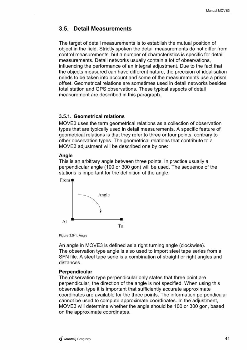
AngleThis is an arbitrary angle between three points. In practice usually aperpendicular angle (100 or 300 gon) will be used. The sequence of thestations is important for the definition of the angle:
AtTo
From
Angle
Figure 3.5-1, Angle
An angle in MOVE3 is defined as a right turning angle (clockwise).The observation type angle is also used to import steel tape series from aSFN file. A steel tape serie is a combination of straight or right angles anddistances.
PerpendicularThe observation type perpendicular only states that three point areperpendicular, the direction of the angle is not specified. When using thisobservation type it is important that sufficiently accurate approximatecoordinates are available for the three points. The information perpendicularcannot be used to compute approximate coordinates. In the adjustment,MOVE3 will determine whether the angle should be 100 or 300 gon, basedon the approximate coordinates.
Detail Measurements Manual MOVE3
@ Grontmij Geogroep 45
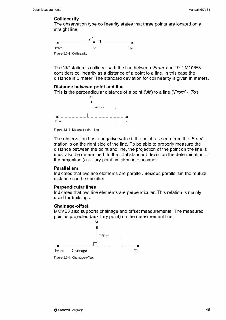
CollinearityThe observation type collinearity states that three points are located on astraight line:
At ToFromFigure 3.5-2, Collinearity
The ‘At’ station is collinear with the line between ‘From’ and ‘To’. MOVE3considers collinearity as a distance of a point to a line, in this case thedistance is 0 meter. The standard deviation for collinearity is given in meters.
Distance between point and lineThis is the perpendicular distance of a point (‘At’) to a line (‘From’ - ‘To’).
At
ToFrom
distance +
-Figure 3.5-3, Distance point - line
The observation has a negative value if the point, as seen from the ‘From’station is on the right side of the line. To be able to properly measure thedistance between the point and line, the projection of the point on the line ismust also be determined. In the total standard deviation the determination ofthe projection (auxiliary point) is taken into account.
ParallelismIndicates that two line elements are parallel. Besides parallelism the mutualdistance can be specified.
Perpendicular linesIndicates that two line elements are perpendicular. This relation is mainlyused for buildings.
Chainage-offsetMOVE3 also supports chainage and offset measurements. The measuredpoint is projected (auxiliary point) on the measurement line.
At
ToFrom Chainage
Offset +
_Figure 3.5-4, Chainage-offset
Detail Measurements Manual MOVE3
@ Grontmij Geogroep 46
3.5.2. Precision of idealisationIt is important in detail adjustments to take into account the precision ofidealisation . The precision of idealisation is the precision of identifying apoint in the field. Corners of buildings are easy to identify in the field, but it israther difficult to identify the centre or the side of a ditch. The precision ofidealisation is independent of the type of measurement, it is a feature of themeasured point (object).To specify the precision of idealisation, use can be made of the classes intable 3.5-1.
Class Classes idealisation Standarddeviationidealisation
benchmark, wall (hard topography) 0.00 - 0.02 m 0.02 m
pavement, street furniture, drain hole 0.01 - 0.03 m 0.03 m
fence 0.02 - 0.05 m 0.05 m
hedge, drain 0.05 - 0.10 m 0.10 m
ditch 0.10 - 0.20 m 0.20 m
non classified points > 0.20 m 0.32 mtable 3.5-1 : Classes for precision of idealisation
The specified precision of idealisation is used to compute the total standarddeviation of observations, similar to the centring error. The precision ofidealisation can also be used to specify a different centring error for eachindividual station.
3.5.3. Eccentric measurementIf the prism cannot be located at the detail point to be measured, an offsetmust be measured by tape. The prism can be positioned fore or after or leftor right of the detail point. The distance of the detail point to the prism ismeasured by tape. Prior to the adjustment the eccentric measures will beused to compute derived observations. To compute the total standarddeviation the standard deviation of the tape measurement and thedetermination of the correct location of the prism (perpendicular) are takeninto account.
Prism
Prism
Setup
1.00m Backw
-0.50m Left
-1.50m Forew
1.50m Right
Figure 3.5-5, Eccentric measurement

Detail Measurements Manual MOVE3
@ Grontmij Geogroep 47
For more information on detail adjustments please refer to HTW 1996 (inDutch), chapter 6, Detailmeting.

Manual MOVE3
@ Grontmij Geogroep 48
4. Quality Control
Manual MOVE3
@ Grontmij Geogroep 49
4.1. IntroductionIt is important for a surveyor, as for any other professional, to assess andcontrol the quality of his work. The reasons for this are obvious:• the work will have to meet certain requirements, so it is essential to be
able to assess whether the requirements are met;• when for some structural (bad design) or incidental reason (observation
error) the requirements are not met, tools must be available to improve thesituation.
Knowing about the costly consequences of ill-designed networks orundetected errors, especially when these deficiencies are discovered in anadvanced stage of the survey, it is clear that quality control will save bothtime and money.Quality control has gained importance in survey work due to the instrumentaldevelopments in recent years. Modern total stations and GPS receivers arecapable of producing a bulk of survey data, thus demanding efficient tools forassessing their sufficiency and accuracy.
Besides instrumental developments, also developments in survey softwarehave opened the way for an increase in the application of quality control. Notlong ago the quality assessment of survey networks by means of reliabilityparameters and statistical testing was reserved for specialists able to operatecomplex computer systems. Nowadays by the introduction of easy to operatePC based software packages, such as MOVE3, quality control can reachprofessionals on all sorts of different levels.
In this part of the manual quality control for geodetic networks is introducedby means of a review of (the parameters of) precision and reliability,according to the 'Delft Method':• The control of the propagation of random errors, present in the
observations, into the coordinates is measured in terms of precision.• The identification of gross errors and/or biases in the observations and the
control over the sensitivity of the data to these errors and biases ismeasured in terms of reliability.
The descriptions in this chapter are presented at a conceptual level, intendedto give the reader a basic understanding of the process. More informationcan be found in the literature listed in Appendix B.
4.1.1. Adjustment, Precision, Reliability and TestingFrom observations carried out in the field, the surveyor will have to computean end result: the coordinates. When redundant observations are available,as it should be, a strategy has to be chosen so as to get a unique andoptimal solution. In geodesy, this strategy usually is the least squaresadjustment. It is based on the following criterion: the sum of squares of theobservational residuals must be minimised. After carrying out a least squaresadjustment we know that we have the best possible solution based on theavailable observations.

Introduction Manual MOVE3
@ Grontmij Geogroep 50
Having determined a solution, it is important for the surveyor to be able toassess the quality of this solution. It is therefore necessary to somehowquantify the quality. By doing so, it can be verified whether the networkmeets the requirements. For example, a surveyor working, as a contractorwill know before delivery whether or not and to what extent the quality of thenetwork meets the client's demands. This works two ways:• a network of poor quality will not be accepted by the client, this will
obviously cause problems;• a network with a far better quality than asked for by the client, is often
undesirable from a cost-efficiency point of view.
The quality of a network, whether already measured or only existing as adesign, can be assessed in terms of precision and reliability. Bothprecision and reliability can be quantified by parameters, which will bediscussed in the following chapters.
By designing a network keeping in mind the demands on precision andreliability, it is possible to control the quality. However, designing a 'perfect'network is not enough. Practice has learned that, mainly due to humanfailures, about 1 in every 100 observations is erroneous. This means that thequality control will have to include some sort of statistical testing, in order toclear the result of possible outliers. The effectiveness of the testing willdepend on the reliability of the network. The more reliable a network is thehigher the probability that outliers will be detected by the testing.
The explanation above should clarify the relationship between the leastsquares adjustment, the precision and reliability concept, and the statisticaltesting. To summarise, one could say that:• the least squares adjustment will produce the best possible result, given
the available data;• the statistical testing checks the result in order to make it 'error-free';• the precision and reliability parameters quantify the quality of the result.
4.1.2. Quality Control in Network PlanningAs explained in the preceding paragraph, the quality of a network can beassessed in terms of precision and reliability. This valuation may take placebefore the start of the actual measurements in the field, namely during theplanning or design of the network. Usually the study of topographic maps ofthe area and reconnaissance in the field precedes the initial design. Theoutcome of the (initial) network design depends on the purpose of thenetwork and on related demands on precision and reliability. Furthermore thelocation of the known stations and the characteristics of the area (e.g.mountainous or flat) can affect the design.A number of general rules of thumb apply for network design:• Aim for a balanced distribution of known stations over the network.
Moreover, the integration of known stations should be acceptable from aprecision and reliability point of view, e.g. an intersection by at least three,preferably four directions.
• Try to include loops in the network, keeping in mind that the lesser thenumber of stations in a loop, the better the reliability. In 2D networks thereliability of loops can be improved by measuring directions and distancesto temporarily monumented auxiliary stations.
• Strive for network sides of approximately equal length.
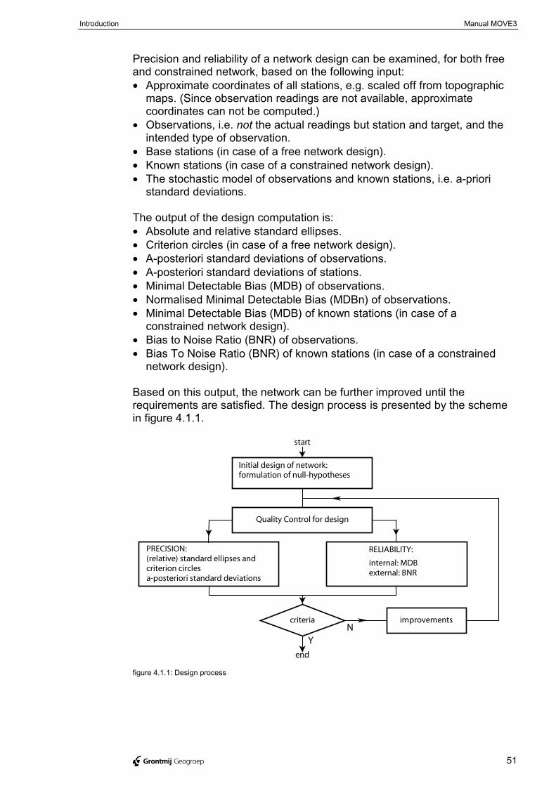
Introduction Manual MOVE3
@ Grontmij Geogroep 51
Precision and reliability of a network design can be examined, for both freeand constrained network, based on the following input:• Approximate coordinates of all stations, e.g. scaled off from topographic
maps. (Since observation readings are not available, approximatecoordinates can not be computed.)
• Observations, i.e. not the actual readings but station and target, and theintended type of observation.
• Base stations (in case of a free network design).• Known stations (in case of a constrained network design).• The stochastic model of observations and known stations, i.e. a-priori
standard deviations.
The output of the design computation is:• Absolute and relative standard ellipses.• Criterion circles (in case of a free network design).• A-posteriori standard deviations of observations.• A-posteriori standard deviations of stations.• Minimal Detectable Bias (MDB) of observations.• Normalised Minimal Detectable Bias (MDBn) of observations.• Minimal Detectable Bias (MDB) of known stations (in case of a
constrained network design).• Bias to Noise Ratio (BNR) of observations.• Bias To Noise Ratio (BNR) of known stations (in case of a constrained
network design).
Based on this output, the network can be further improved until therequirements are satisfied. The design process is presented by the schemein figure 4.1.1.
start
Initial design of network:formulation of null-hypotheses
Quality Control for design
PRECISION:(relative) standard ellipses andcriterion circlesa-posteriori standard deviations
RELIABILITY:
internal: MDBexternal: BNR
criteria
end
improvementsN
Y
figure 4.1.1: Design process
Manual MOVE3
@ Grontmij Geogroep 52
4.2. Least Squares AdjustmentIn this chapter the basic ideas of least squares adjustment are introduced,together with the concepts of mathematical and stochastic models.Furthermore, important notions used in MOVE3 such as approximate values,nuisance parameters, constraints and adjustment in phases, are reviewed.
4.2.1. GeneralIt is common practice for a surveyor to carry out extra measurements whenestablishing a geodetic network. This will enable compensation for a possibleloss of observations and, more important, the quality of the network can beimproved. As a consequence of the extra measurements there is no longer aunique solution which satisfies the conditions in the network exactly (e.g. theangles of a triangle should add up to 200 gon). Therefore a method isneeded to correct the observations in order to make them meet theconditions. The amount by which each observation has to be corrected iscalled the observation residual. The least squares adjustment method willmake the observations fit into the model by minimising the sum of squares ofthe observation residuals. The residuals are referred to as least squarescorrections.
Any least squares adjustment model consists of two equally importantcomponents: the mathematical model and the stochastic model. Themathematical model is a set of relations between the observations and theunknowns. The stochastic model describes the expected error distribution ofthe observations.
4.2.2. Mathematical ModelUsually in a survey the observables themselves are not the quantities whichwe are aiming for. Instead, we use the observations to determine unknownparameters, e.g. the coordinates of stations in a network. The observationsare expressed as a function of the parameters in the so-called functional ormathematical model.
In some cases the model representing the relations between the observablesand the unknown parameters is very simple. The relation, for instance, in a1-dimensional levelling problem between the observed height differencesand the unknown heights is simply linear:
∆hij = hj - hi
More complicated is the case for a GPS network where the unknowns arecoordinates (X, Y, Z) to be determined in a reference system different fromthat of the observed baselines ∆X:
∆Xij = function (α, β, γ, µ, Xi, Yi, Zi, Xj, Yj, Zj)with
α, β, γ, µ as transformation parameters.
Least Squares Adjustment Manual MOVE3
@ Grontmij Geogroep 53
As the least squares approach requires linear equations, the model abovemust be linearised. Usually this means that a number of iterations areneeded to reach a solution. Moreover, approximate values for thecoordinate unknowns in the adjustment are required. Bad approximatevalues can lead to an increasing number of iterations or, in the worst case, tono convergence at all.
Since coordinates are our main concern, other unknowns in themathematical model are not always useful for us. Unknowns such as thetransformation parameters mentioned above, are called additional ornuisance parameters. Typical nuisance parameters are transformationparameters, scale factors, azimuth offsets, orientation unknowns andrefraction coefficients. Some of these parameters can be kept fixed at acertain value, in which case they are not corrected in the adjustment.Whether or not to fix parameters is a question that can not easily beanswered. We must always be careful to avoid overconstraining as well asoverparameterisation. The introduction of refraction coefficients for example,could result in the absorption of systematic effects, which are not caused byrefraction. However, ignoring the refraction, when in fact it does have aninfluence on the measurements, will cause an equally unfavourable effect.The success of what could be referred to as 'tuning' of the model will dependlargely on the user's expertise.
Scale factors are especially important in 'tuning' the model. In MOVE3 up to10 scale factors are allowed per network, but in most cases one scale factoris sufficient. The aim of introducing a free scale factor in the adjustment is toovercome a possible bias in the internal scale of the measurementequipment and, in more general terms, to prevent the overconstraining of thenetwork in a free network adjustment. A free scale factor will 'shrink' or 'blowup' the network in order to make it fit onto the known stations in constrainedadjustments. As a result, in some situations a free scale factor may obstructthe statistical testing of known stations. An outlier in the coordinates of aknown station could remain undetected when, due to the 'shrink' or 'blow up'effect, the network can still be forced to fit the known stations without anyrejections. The outlier in question is absorbed by the scale factor, which willconsequently have a value distinctly different from 1.0. It is thereforerecommended to examine the value of the scale factor after the adjustmentand, in case of doubt, to rerun the adjustment with a fixed scale.
An adjustment will fail when the mathematical model, as represented by thedesign matrix and normal matrix (see paragraph 4.2.5, Formulae), issingular. Singularity is caused by:• an ill-posed problem;• an improperly formulated model.
The problem may be ill-posed because we expect too much from theobservations, or because too few observations were included. An example ofan ill-posed problem is the determination of the 2D coordinates of anunknown station by a single horizontal direction from another station. Amodel is improperly formulated, when too many parameters are included. Ingeneral an improperly formulated model does not correctly represent theexisting physical reality.
Least Squares Adjustment Manual MOVE3
@ Grontmij Geogroep 54
For computerised solutions to least squares problems the ill-conditioning ofthe normal matrix N could result in singularity. Singularity is the limiting caseof ill-conditioning. An ill-conditioned matrix can become 'singular' as a resultof the internal accuracy limits of the computer hardware. An example of anill-conditioned problem is the intersection of a station by two or more nearlyparallel directions.
Apart from the problems mentioned above, an adjustment cannot be solvedunless the location, orientation and scale of the network are established, i.e.a 'datum' must be defined. This is done by imposing constraints on thesolution. The minimum number of constraints depends on the dimension ofthe network:• In case of a 3D network there are 3 translations, 3 rotations and 1 scale
factor. The singularity is then eliminated by fixing at least 7 coordinates of3 stations (X East1, Y North1, h1, X East2, Y North2, h2, h3).
• In case of a 2D network there are 2 translations, 1 rotation and 1 scalefactor. The singularity is then phased out by fixing at least 2 base stations(X East1, Y North1, X East2, Y North2).
• In case of a 1D network the location of the network is determined bykeeping one height fixed.
4.2.3. Stochastic ModelA geodetic observable, such as a direction, distance or height difference, is arandom or stochastic variable. A stochastic variable cannot be described bya single and exact value because there is an amount of uncertainty involvedin the measurement process. For example, repeatedly measuring thedistance between two stations will result in a range of different values. Thisvariation is accounted for by a probability distribution. This means that inaddition to the mathematical model, it is necessary to formulate a secondmodel which describes the stochastic deviations of the observations; thestochastic model.
For geodetic observables a normal probability distribution is assumed (figure4.2.1). This distribution is based on the mean µµµµ and the standard deviationσσσσ.
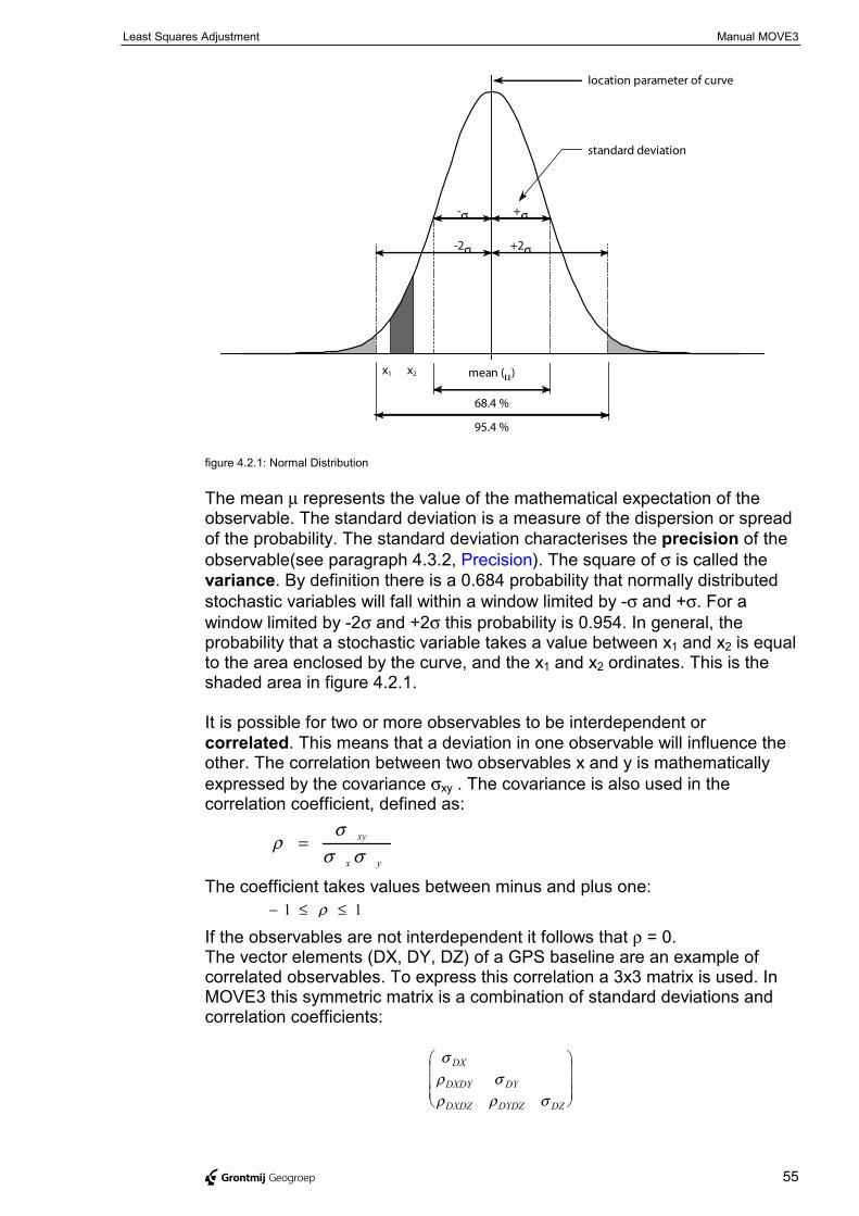
Least Squares Adjustment Manual MOVE3
@ Grontmij Geogroep 55
location parameter of curve
standard deviation
mean (µ)
68.4 %
95.4 %
x1 x2
-2σ +2σ
-σ +σ
figure 4.2.1: Normal Distribution
The mean µ represents the value of the mathematical expectation of theobservable. The standard deviation is a measure of the dispersion or spreadof the probability. The standard deviation characterises the precision of theobservable(see paragraph 4.3.2, Precision). The square of σ is called thevariance. By definition there is a 0.684 probability that normally distributedstochastic variables will fall within a window limited by -σ and +σ. For awindow limited by -2σ and +2σ this probability is 0.954. In general, theprobability that a stochastic variable takes a value between x1 and x2 is equalto the area enclosed by the curve, and the x1 and x2 ordinates. This is theshaded area in figure 4.2.1.
It is possible for two or more observables to be interdependent orcorrelated. This means that a deviation in one observable will influence theother. The correlation between two observables x and y is mathematicallyexpressed by the covariance σxy . The covariance is also used in thecorrelation coefficient, defined as:
yx
xy
σσσ
ρ =
The coefficient takes values between minus and plus one:11 ≤≤− ρ
If the observables are not interdependent it follows that ρ = 0.The vector elements (DX, DY, DZ) of a GPS baseline are an example ofcorrelated observables. To express this correlation a 3x3 matrix is used. InMOVE3 this symmetric matrix is a combination of standard deviations andcorrelation coefficients:
σρ σρ ρ σ
DX
DXDY DY
DXDZ DYDZ DZ
�
�
���
�
�
���
Least Squares Adjustment Manual MOVE3
@ Grontmij Geogroep 56
For practical reasons, and because their influence in the adjustment islimited, correlations are sometimes disregarded.
In essence the stochastic model consists of a choice for the probabilitydistribution of the observables. Practically this means that for eachobservable a standard deviation σ is chosen. The value for σ is based onknowledge about the measurement process (conditions in the field, type ofinstrument) and experience. The standard deviation of most observables issupposed to consist of an absolute part, and a relative part. In the relativepart the dependence on the distance between station and target, whichcharacterises the precision of most observables, is accounted for. The thusdefined standard deviations are entered in the variance-covariance matrix Qy(see paragraph 4.2.5, Formulae). The precision of the unknowns in theadjustment depends on the precision of the observables given in Qy, and onthe propagation of this precision through the mathematical model.
4.2.4. Free and Constrained AdjustmentsThe adjustment of a network is usually subdivided into two separate steps orphases:• free network adjustment;• constrained adjustment.This approach is intended to separate the testing of observations and knownstations.
A free network can be defined as a network of which the geometrical layoutis determined by the observations only. The position, scale and orientation ofthe network are fixed by a minimum number of constraints, through the basestations. Thus, the base stations impose no extra constraints on theadjustment solution. In a free network adjustment the emphasis is laid on thequality control of the observations, rather than on the computation ofcoordinates. Selecting other stations to fix the position, scale and orientationwill change the coordinates, but not the statistical testing as implemented inMOVE3.
Having eliminated possible outliers in the observations in the free networkadjustment, the network can be connected to the known stations. This doesimpose extra constraints on the solution. Now the emphasis is on theanalysis of the known stations and on the computation of the finalcoordinates. There are three types of constrained adjustments:• In a pseudo least squares constrained adjustment the coordinates of the
known stations are kept at their original value, i.e. they do not receive aleast squares correction. Also the standard deviations of the knownstations do not change in the adjustment.
• In a weighted constrained adjustment however, the known stations doreceive a correction. The known stations are considered as observations,with their respective standard deviations.
• In an absolute constrained adjustment the coordinates of the knownstations are kept at their original value, i.e. they do not receive a leastsquares correction. The standard deviations of the known stations will bekept 0 during the adjustment. The known stations are considered asobservations, with standard deviations 0.
Least Squares Adjustment Manual MOVE3
@ Grontmij Geogroep 57
The choice of the constrained adjustment type does not influence the testingof the known stations. For testing the known stations in all cases thespecified standard deviations will be used.
4.2.5. FormulaeThe (linearised) mathematical model is:
y = Ax +e + awith
y = (m) vector of observations;e = (m) vector of corrections;A = (m x n) design matrix;x = (n) vector of unknowns;a = (m) vector of constants.
The stochastic model is:
Q Q Py = = −σσ
22
11
withQy= (m x m) variance-covariance matrix;
σ² = a-priori variance-of-unit-weight;Q = (m x m) weight coefficient matrix;P = (m x m) weight matrix.
The least squares criterion is:
etPe = minimum
The solution is:
� ( ) ( )x A PA A P y at t= −−1
se P em n
t2 =
−
with(At P A) = N = (n x n) normal matrix;s² = a-posteriori variance-of-unit-weight.
The variance-covariance matrix of the unknowns:
Q Nx� = −σ 2 1
! The a-priori σσσσ² is used, not the a-posteriori s²

Least Squares Adjustment Manual MOVE3
@ Grontmij Geogroep 58
In case of a linearised mathematical model, the solution for the vector ofunknowns x is available after a series of iterative updates ∆ �x of theapproximate values x0:
� �x x x= +0 ∆
After each iteration, the new solution is compared with the previous one. Ifthe difference between the two solutions satisfies the iteration criterion, theiteration process is ended and the last solution is regarded as final.
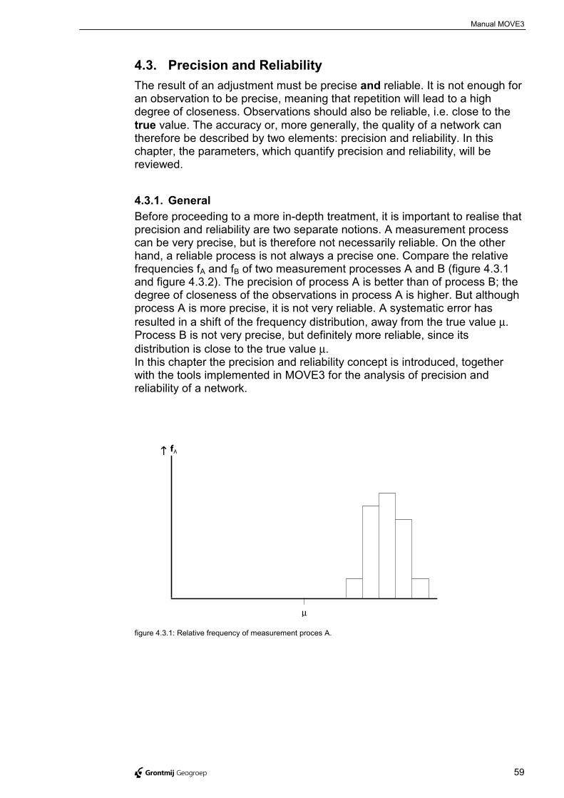
Manual MOVE3
@ Grontmij Geogroep 59
4.3. Precision and ReliabilityThe result of an adjustment must be precise and reliable. It is not enough foran observation to be precise, meaning that repetition will lead to a highdegree of closeness. Observations should also be reliable, i.e. close to thetrue value. The accuracy or, more generally, the quality of a network cantherefore be described by two elements: precision and reliability. In thischapter, the parameters, which quantify precision and reliability, will bereviewed.
4.3.1. GeneralBefore proceeding to a more in-depth treatment, it is important to realise thatprecision and reliability are two separate notions. A measurement processcan be very precise, but is therefore not necessarily reliable. On the otherhand, a reliable process is not always a precise one. Compare the relativefrequencies fA and fB of two measurement processes A and B (figure 4.3.1and figure 4.3.2). The precision of process A is better than of process B; thedegree of closeness of the observations in process A is higher. But althoughprocess A is more precise, it is not very reliable. A systematic error hasresulted in a shift of the frequency distribution, away from the true value µ.Process B is not very precise, but definitely more reliable, since itsdistribution is close to the true value µ.In this chapter the precision and reliability concept is introduced, togetherwith the tools implemented in MOVE3 for the analysis of precision andreliability of a network.
µ
↑↑↑↑ fA
figure 4.3.1: Relative frequency of measurement proces A.
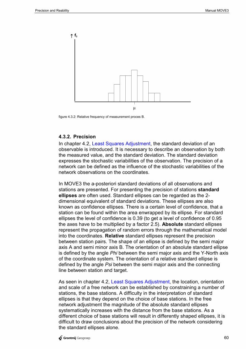
Precision and Reability Manual MOVE3
@ Grontmij Geogroep 60
µ
↑↑↑↑ fB
figure 4.3.2: Relative frequency of measurement proces B.
4.3.2. PrecisionIn chapter 4.2, Least Squares Adjustment, the standard deviation of anobservable is introduced. It is necessary to describe an observation by boththe measured value, and the standard deviation. The standard deviationexpresses the stochastic variabilities of the observation. The precision of anetwork can be defined as the influence of the stochastic variabilities of thenetwork observations on the coordinates.
In MOVE3 the a-posteriori standard deviations of all observations andstations are presented. For presenting the precision of stations standardellipses are often used. Standard ellipses can be regarded as the 2-dimensional equivalent of standard deviations. These ellipses are alsoknown as confidence ellipses. There is a certain level of confidence, that astation can be found within the area enwrapped by its ellipse. For standardellipses the level of confidence is 0.39 (to get a level of confidence of 0.95the axes have to be multiplied by a factor 2.5). Absolute standard ellipsesrepresent the propagation of random errors through the mathematical modelinto the coordinates. Relative standard ellipses represent the precisionbetween station pairs. The shape of an ellipse is defined by the semi majoraxis A and semi minor axis B. The orientation of an absolute standard ellipseis defined by the angle Phi between the semi major axis and the Y-North axisof the coordinate system. The orientation of a relative standard ellipse isdefined by the angle Psi between the semi major axis and the connectingline between station and target.
As seen in chapter 4.2, Least Squares Adjustment, the location, orientationand scale of a free network can be established by constraining a number ofstations, the base stations. A difficulty in the interpretation of standardellipses is that they depend on the choice of base stations. In the freenetwork adjustment the magnitude of the absolute standard ellipsessystematically increases with the distance from the base stations. As adifferent choice of base stations will result in differently shaped ellipses, it isdifficult to draw conclusions about the precision of the network consideringthe standard ellipses alone.
Precision and Reability Manual MOVE3
@ Grontmij Geogroep 61
Therefore in the free network adjustment so-called criterion circles areconstructed. Criterion circles determine a theoretical model, representing ahomogeneous precision of the network, computed with a similar choice ofbase stations. It is obvious that the ratio of the semi major axis of thestandard ellipse A and the radius of the criterion circle R, A/R, is of moreimportance than the individual values. This ratio, however, still depends to acertain extend on the chosen base stations. Strictly speaking, this alsoapplies for the ratio A/R belonging to relative standard ellipses. In mostcases however, the latter quantity behaves practically independent of thebase stations.
The criterion model, expressed by the criterion circles, is regulated by theparameters C0 and C1. The C0 parameter controls the absolute part of theprecision. The C1 parameter, the relative part, is a coefficient controlling theinfluence of the mutual distance on the relative precision between twostations. Often used empirically established values are: C0 = 0 cm²,C1 = 1 cm²/km.
4.3.3. ReliabilityThe reliability of a network can be described in terms of the sensitivity to thedetection of outliers. Reliability can be subdivided into internal and externalreliability:• Internal reliability is expressed by the Minimal Detectable Bias (MDB).
The MDB presents the size of the smallest possible observation error, stilldetectable by the statistical test (datasnooping) with a probability equal tothe power γ of the test. A large MDB indicates a weakly checkedobservation or coordinate. Thus, the larger the MDB the poorer thereliability. If an observation is not checked at all, no MDB can becomputed and the observation is marked as a 'free observation'. Tocompare the MDB values of different observation types the normalisedMinimal Detectable Bias (MDBn) can be used. By relating the minimaldetectable bias to the deviation of the observation the unit can beeliminated. For uncorrelated observations the normalised minimaldetectable bias is equal to the minimal detectable bias divided by thestandard deviation of the observation.
• Internal reliability can also be expressed in terms of the RedundancyNumber. The (local) Redundancy number presents the contribution of anobservation to the total redundancy. The local redundancy number lies inthe closed interval 0≤ri≤1 (in the MOVE3 output file it is presented in apercentage 0-100%). The correction multiplied by the redundancynumber presents the size of the observation error. A large redundancynumber indicates a strongly checked observation. Thus, the smaller theredundancy number the poorer the reliability. The redundancy numberequals zero if the observation is not checked at all ('free observation'). Thesum of the local redundancy numbers equals the total redundancy.
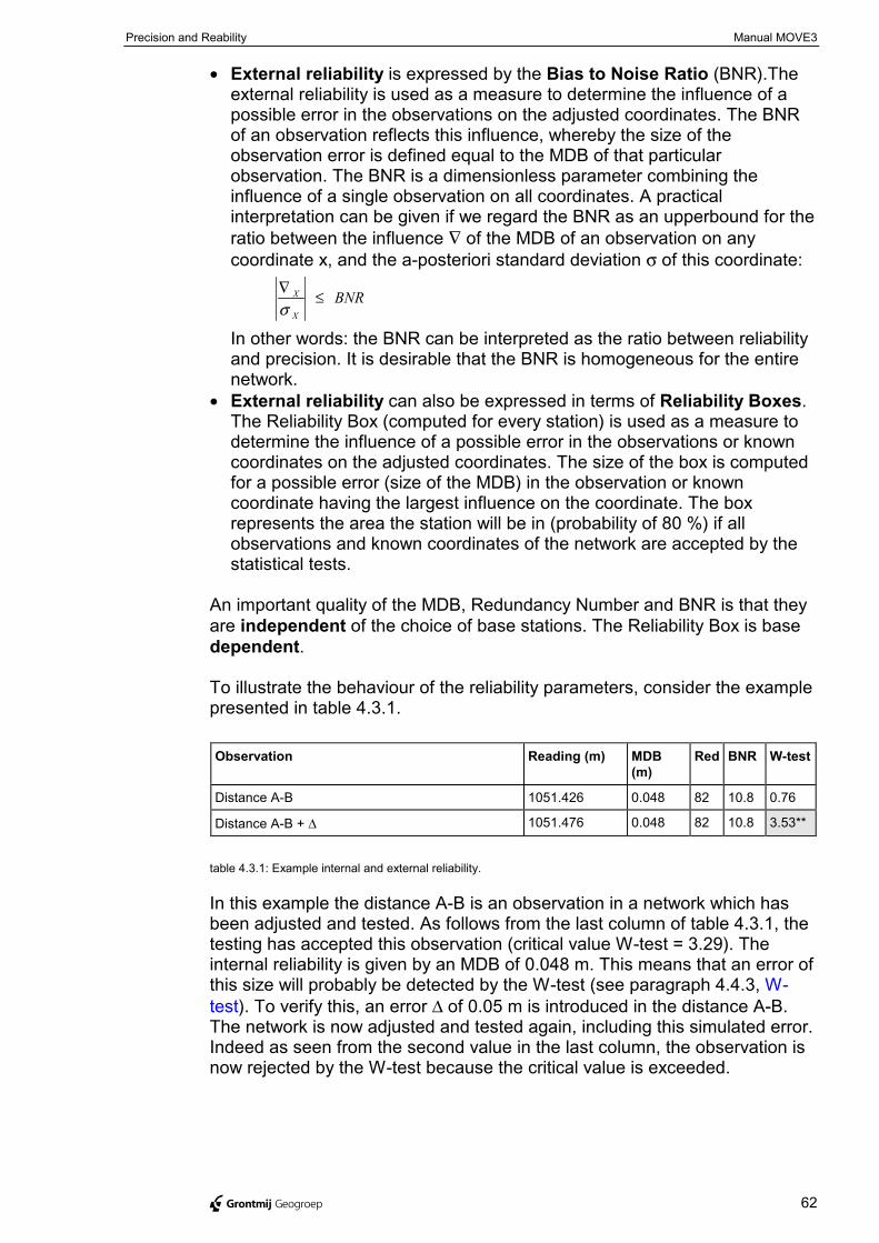
Precision and Reability Manual MOVE3
@ Grontmij Geogroep 62
• External reliability is expressed by the Bias to Noise Ratio (BNR).Theexternal reliability is used as a measure to determine the influence of apossible error in the observations on the adjusted coordinates. The BNRof an observation reflects this influence, whereby the size of theobservation error is defined equal to the MDB of that particularobservation. The BNR is a dimensionless parameter combining theinfluence of a single observation on all coordinates. A practicalinterpretation can be given if we regard the BNR as an upperbound for theratio between the influence ∇ of the MDB of an observation on anycoordinate x, and the a-posteriori standard deviation σ of this coordinate:
BNRX
X ≤∇σ
In other words: the BNR can be interpreted as the ratio between reliabilityand precision. It is desirable that the BNR is homogeneous for the entirenetwork.
• External reliability can also be expressed in terms of Reliability Boxes.The Reliability Box (computed for every station) is used as a measure todetermine the influence of a possible error in the observations or knowncoordinates on the adjusted coordinates. The size of the box is computedfor a possible error (size of the MDB) in the observation or knowncoordinate having the largest influence on the coordinate. The boxrepresents the area the station will be in (probability of 80 %) if allobservations and known coordinates of the network are accepted by thestatistical tests.
An important quality of the MDB, Redundancy Number and BNR is that theyare independent of the choice of base stations. The Reliability Box is basedependent.
To illustrate the behaviour of the reliability parameters, consider the examplepresented in table 4.3.1.
Observation Reading (m) MDB(m)
Red BNR W-test
Distance A-B 1051.426 0.048 82 10.8 0.76
Distance A-B + ∆ 1051.476 0.048 82 10.8 3.53**
table 4.3.1: Example internal and external reliability.
In this example the distance A-B is an observation in a network which hasbeen adjusted and tested. As follows from the last column of table 4.3.1, thetesting has accepted this observation (critical value W-test = 3.29). Theinternal reliability is given by an MDB of 0.048 m. This means that an error ofthis size will probably be detected by the W-test (see paragraph 4.4.3, W-test). To verify this, an error ∆ of 0.05 m is introduced in the distance A-B.The network is now adjusted and tested again, including this simulated error.Indeed as seen from the second value in the last column, the observation isnow rejected by the W-test because the critical value is exceeded.

Precision and Reability Manual MOVE3
@ Grontmij Geogroep 63
The external reliability is given by a BNR of 10.8. This means that theinfluence of the MDB of 0.048 m on any coordinate in the network is smallerthan 10.8 times the a-posteriori standard deviation of the coordinate. Forgeneral-purpose networks it is desirable to have a homogeneous externalreliability. The network in the example is considered as homogeneous, whenthe BNR values of all observations are on the same level. Alternatively thenetwork is inhomogeneous when the BNR of e.g. distance A-B stronglyexceeds the BNR of other observations in the network. In that case thenetwork is unstable or inhomogeneous, i.e. the reliability depends mainly onthe correctness of one single observation.
Manual MOVE3
@ Grontmij Geogroep 64
4.4. Statistical TestingThe aim of statistical testing is to check whether the mathematical andstochastic models (see paragraph 4.2, Least Squares Adjustment) are acorrect representation of 'reality'. Furthermore, it is important to detectpossible outliers (blunders) in the observations, which could ruin theachievable accuracy. This makes statistical testing essential for the processof quality control. The statistical testing presented here is carried out togetherwith the least squares adjustment. It is based on the analysis of leastsquares residuals. The detection of blunders can also be carried out prior tothe adjustment by e.g. a check on loop misclosures or on erroneous stationnumbering. These checks are regarded as part of the pre-processing andare not further discussed here.
Three types of statistical tests are implemented in MOVE3: the F-test, W-testand T-test. In this chapter the testing procedures are explained, preceded bya general description of hypothesis testing. In the final paragraphs attentionis paid to the interpretation of the testing results and estimated errors.
4.4.1. GeneralThe mathematical and stochastic models are based on a set of assumptions.This set is called a statistical hypothesis. Different assumptions will result indifferent hypotheses. Statistical testing is used to verify the hypotheses. Aspecial set of assumptions is referred to as the null-hypothesis H0. Thishypothesis implies that:• there are no gross errors (blunders) present in the observations;• the mathematical model gives a correct description of the relations
between the observations and the unknown parameters;• the chosen stochastic model for the observations appropriately describes
the stochastic properties of the observations.
It is clear that there are two possible outcomes for the testing of ahypothesis: acceptance or rejection. A specific cut-off point or critical valuedecides over acceptance and rejection. The critical values establish awindow of acceptance. The further beyond this window, the less certain theset of assumptions is satisfied. Critical values are determined by the choiceof a level of significance α. The probability that the critical value isexceeded, although the set of assumptions is valid, is equal to α. In otherwords, α is the probability of an incorrect rejection. Alternatively thecomplementary level of confidence 1-α, is a measure of the confidence onecan have in the decision.
In the testing of the null-hypothesis H0 there are two unfavourable situationsthat might occur:• Rejection of H0 while in fact it is true. The probability of this situation
occurring is equal to the significance level α. This situation is called aType I error (table 4.4.1).
• Acceptance of H0 while in fact it is false. The probability of this situationoccurring is 1-γ, with γ the power of the test. This situation is called aType II error (table 4.4.1).
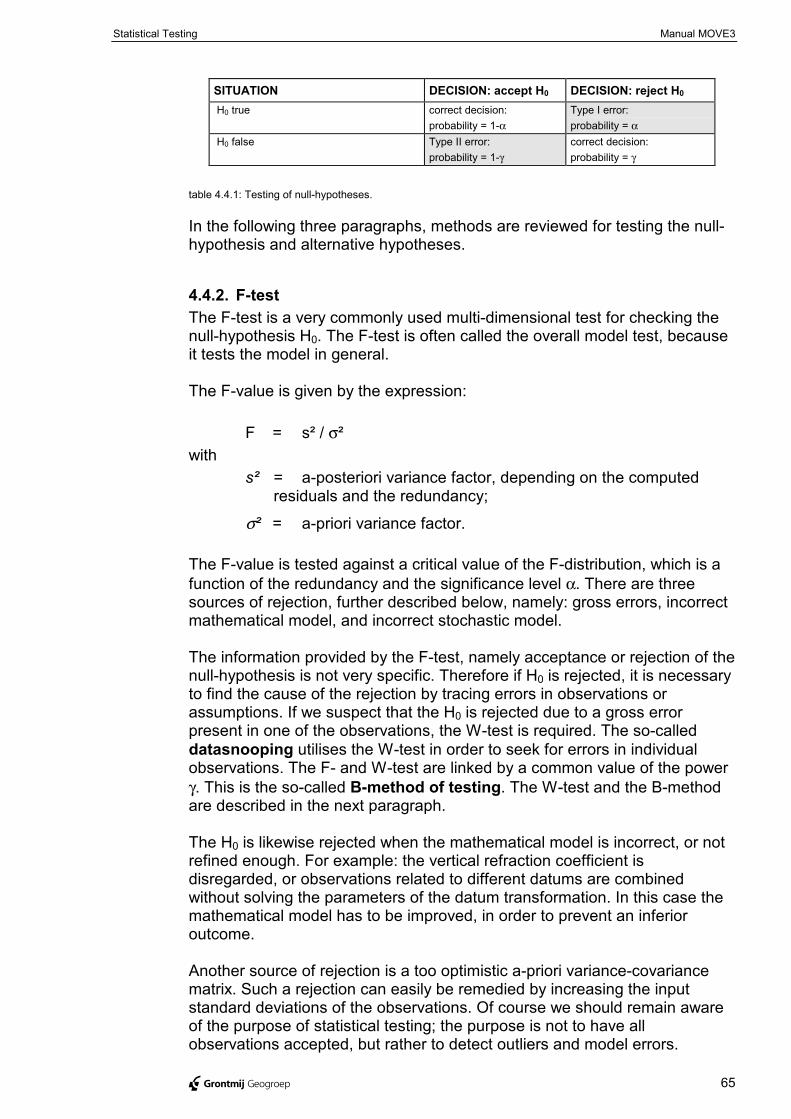
Statistical Testing Manual MOVE3
@ Grontmij Geogroep 65
SITUATION DECISION: accept H0 DECISION: reject H0
H0 true correct decision:probability = 1-α
Type I error:probability = α
H0 false Type II error:probability = 1-γ
correct decision:probability = γ
table 4.4.1: Testing of null-hypotheses.
In the following three paragraphs, methods are reviewed for testing the null-hypothesis and alternative hypotheses.
4.4.2. F-testThe F-test is a very commonly used multi-dimensional test for checking thenull-hypothesis H0. The F-test is often called the overall model test, becauseit tests the model in general.
The F-value is given by the expression:
F = s² / σ²with
s² = a-posteriori variance factor, depending on the computedresiduals and the redundancy;
σ² = a-priori variance factor.
The F-value is tested against a critical value of the F-distribution, which is afunction of the redundancy and the significance level α. There are threesources of rejection, further described below, namely: gross errors, incorrectmathematical model, and incorrect stochastic model.
The information provided by the F-test, namely acceptance or rejection of thenull-hypothesis is not very specific. Therefore if H0 is rejected, it is necessaryto find the cause of the rejection by tracing errors in observations orassumptions. If we suspect that the H0 is rejected due to a gross errorpresent in one of the observations, the W-test is required. The so-calleddatasnooping utilises the W-test in order to seek for errors in individualobservations. The F- and W-test are linked by a common value of the powerγ. This is the so-called B-method of testing. The W-test and the B-methodare described in the next paragraph.
The H0 is likewise rejected when the mathematical model is incorrect, or notrefined enough. For example: the vertical refraction coefficient isdisregarded, or observations related to different datums are combinedwithout solving the parameters of the datum transformation. In this case themathematical model has to be improved, in order to prevent an inferioroutcome.
Another source of rejection is a too optimistic a-priori variance-covariancematrix. Such a rejection can easily be remedied by increasing the inputstandard deviations of the observations. Of course we should remain awareof the purpose of statistical testing; the purpose is not to have allobservations accepted, but rather to detect outliers and model errors.
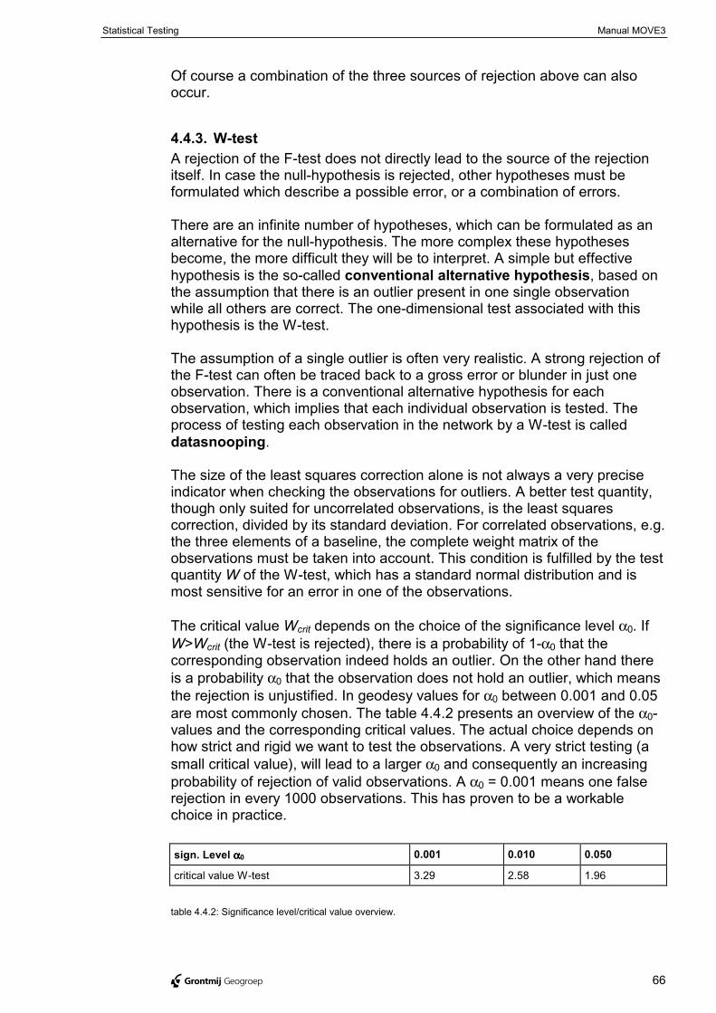
Statistical Testing Manual MOVE3
@ Grontmij Geogroep 66
Of course a combination of the three sources of rejection above can alsooccur.
4.4.3. W-testA rejection of the F-test does not directly lead to the source of the rejectionitself. In case the null-hypothesis is rejected, other hypotheses must beformulated which describe a possible error, or a combination of errors.
There are an infinite number of hypotheses, which can be formulated as analternative for the null-hypothesis. The more complex these hypothesesbecome, the more difficult they will be to interpret. A simple but effectivehypothesis is the so-called conventional alternative hypothesis, based onthe assumption that there is an outlier present in one single observationwhile all others are correct. The one-dimensional test associated with thishypothesis is the W-test.
The assumption of a single outlier is often very realistic. A strong rejection ofthe F-test can often be traced back to a gross error or blunder in just oneobservation. There is a conventional alternative hypothesis for eachobservation, which implies that each individual observation is tested. Theprocess of testing each observation in the network by a W-test is calleddatasnooping.
The size of the least squares correction alone is not always a very preciseindicator when checking the observations for outliers. A better test quantity,though only suited for uncorrelated observations, is the least squarescorrection, divided by its standard deviation. For correlated observations, e.g.the three elements of a baseline, the complete weight matrix of theobservations must be taken into account. This condition is fulfilled by the testquantity W of the W-test, which has a standard normal distribution and ismost sensitive for an error in one of the observations.
The critical value Wcrit depends on the choice of the significance level α0. IfW>Wcrit (the W-test is rejected), there is a probability of 1-α0 that thecorresponding observation indeed holds an outlier. On the other hand thereis a probability α0 that the observation does not hold an outlier, which meansthe rejection is unjustified. In geodesy values for α0 between 0.001 and 0.05are most commonly chosen. The table 4.4.2 presents an overview of the α0-values and the corresponding critical values. The actual choice depends onhow strict and rigid we want to test the observations. A very strict testing (asmall critical value), will lead to a larger α0 and consequently an increasingprobability of rejection of valid observations. A α0 = 0.001 means one falserejection in every 1000 observations. This has proven to be a workablechoice in practice.
sign. Level αααα0 0.001 0.010 0.050
critical value W-test 3.29 2.58 1.96
table 4.4.2: Significance level/critical value overview.
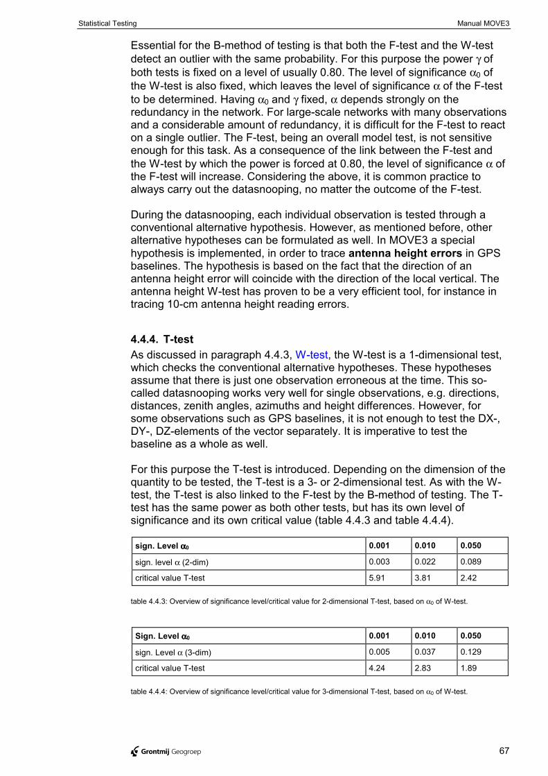
Statistical Testing Manual MOVE3
@ Grontmij Geogroep 67
Essential for the B-method of testing is that both the F-test and the W-testdetect an outlier with the same probability. For this purpose the power γ ofboth tests is fixed on a level of usually 0.80. The level of significance α0 ofthe W-test is also fixed, which leaves the level of significance α of the F-testto be determined. Having α0 and γ fixed, α depends strongly on theredundancy in the network. For large-scale networks with many observationsand a considerable amount of redundancy, it is difficult for the F-test to reacton a single outlier. The F-test, being an overall model test, is not sensitiveenough for this task. As a consequence of the link between the F-test andthe W-test by which the power is forced at 0.80, the level of significance α ofthe F-test will increase. Considering the above, it is common practice toalways carry out the datasnooping, no matter the outcome of the F-test.
During the datasnooping, each individual observation is tested through aconventional alternative hypothesis. However, as mentioned before, otheralternative hypotheses can be formulated as well. In MOVE3 a specialhypothesis is implemented, in order to trace antenna height errors in GPSbaselines. The hypothesis is based on the fact that the direction of anantenna height error will coincide with the direction of the local vertical. Theantenna height W-test has proven to be a very efficient tool, for instance intracing 10-cm antenna height reading errors.
4.4.4. T-testAs discussed in paragraph 4.4.3, W-test, the W-test is a 1-dimensional test,which checks the conventional alternative hypotheses. These hypothesesassume that there is just one observation erroneous at the time. This so-called datasnooping works very well for single observations, e.g. directions,distances, zenith angles, azimuths and height differences. However, forsome observations such as GPS baselines, it is not enough to test the DX-,DY-, DZ-elements of the vector separately. It is imperative to test thebaseline as a whole as well.
For this purpose the T-test is introduced. Depending on the dimension of thequantity to be tested, the T-test is a 3- or 2-dimensional test. As with the W-test, the T-test is also linked to the F-test by the B-method of testing. The T-test has the same power as both other tests, but has its own level ofsignificance and its own critical value (table 4.4.3 and table 4.4.4).
sign. Level αααα0 0.001 0.010 0.050
sign. level α (2-dim) 0.003 0.022 0.089
critical value T-test 5.91 3.81 2.42
table 4.4.3: Overview of significance level/critical value for 2-dimensional T-test, based on α0 of W-test.
Sign. Level αααα0 0.001 0.010 0.050
sign. Level α (3-dim) 0.005 0.037 0.129
critical value T-test 4.24 2.83 1.89
table 4.4.4: Overview of significance level/critical value for 3-dimensional T-test, based on α0 of W-test.
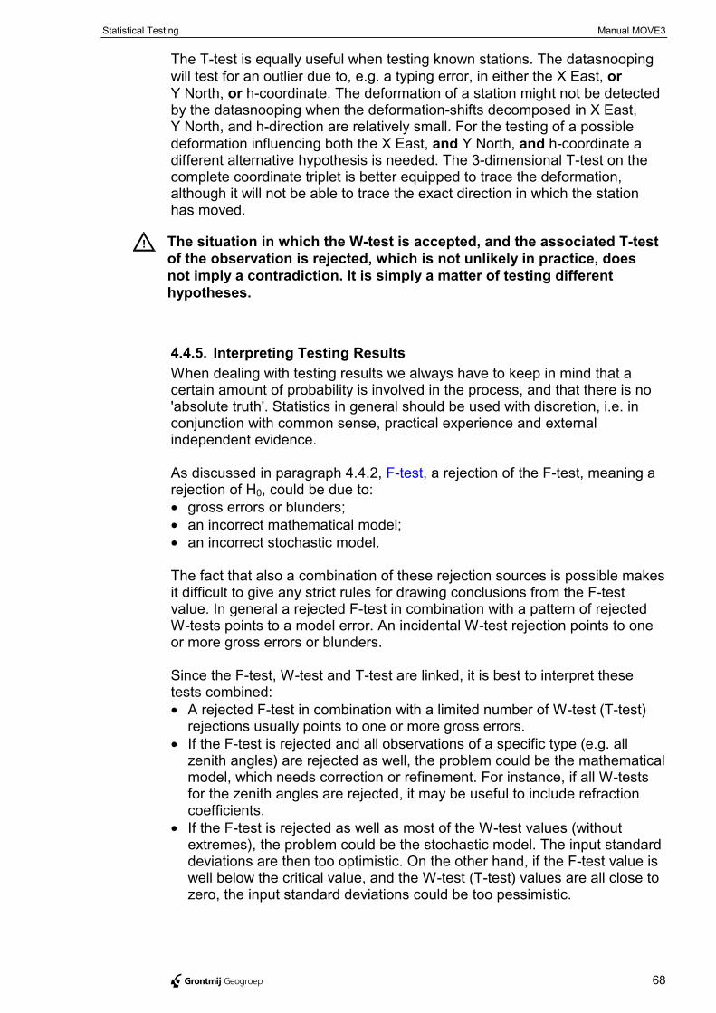
Statistical Testing Manual MOVE3
@ Grontmij Geogroep 68
The T-test is equally useful when testing known stations. The datasnoopingwill test for an outlier due to, e.g. a typing error, in either the X East, orY North, or h-coordinate. The deformation of a station might not be detectedby the datasnooping when the deformation-shifts decomposed in X East,Y North, and h-direction are relatively small. For the testing of a possibledeformation influencing both the X East, and Y North, and h-coordinate adifferent alternative hypothesis is needed. The 3-dimensional T-test on thecomplete coordinate triplet is better equipped to trace the deformation,although it will not be able to trace the exact direction in which the stationhas moved.
! The situation in which the W-test is accepted, and the associated T-testof the observation is rejected, which is not unlikely in practice, doesnot imply a contradiction. It is simply a matter of testing differenthypotheses.
4.4.5. Interpreting Testing ResultsWhen dealing with testing results we always have to keep in mind that acertain amount of probability is involved in the process, and that there is no'absolute truth'. Statistics in general should be used with discretion, i.e. inconjunction with common sense, practical experience and externalindependent evidence.
As discussed in paragraph 4.4.2, F-test, a rejection of the F-test, meaning arejection of H0, could be due to:• gross errors or blunders;• an incorrect mathematical model;• an incorrect stochastic model.
The fact that also a combination of these rejection sources is possible makesit difficult to give any strict rules for drawing conclusions from the F-testvalue. In general a rejected F-test in combination with a pattern of rejectedW-tests points to a model error. An incidental W-test rejection points to oneor more gross errors or blunders.
Since the F-test, W-test and T-test are linked, it is best to interpret thesetests combined:• A rejected F-test in combination with a limited number of W-test (T-test)
rejections usually points to one or more gross errors.• If the F-test is rejected and all observations of a specific type (e.g. all
zenith angles) are rejected as well, the problem could be the mathematicalmodel, which needs correction or refinement. For instance, if all W-testsfor the zenith angles are rejected, it may be useful to include refractioncoefficients.
• If the F-test is rejected as well as most of the W-test values (withoutextremes), the problem could be the stochastic model. The input standarddeviations are then too optimistic. On the other hand, if the F-test value iswell below the critical value, and the W-test (T-test) values are all close tozero, the input standard deviations could be too pessimistic.
Statistical Testing Manual MOVE3
@ Grontmij Geogroep 69
Suppose that the datasnooping on the observations in a network hasresulted in a (limited) number of rejections. It is assumed that the rejectionsare not caused by mathematical model errors, and that obvious errors suchas typing mistakes have been fixed. This leaves a number of options:• Remove the corresponding observation.
This is a valid but rather abrupt way of handling rejections. Rememberthat the removal of observations decreases the redundancy, and thereforeinfluences precision and reliability.
• Remeasure the corresponding observation.Remeasuring observations is an obvious but often expensive way toeliminate rejections, especially when the fieldwork is already completed. Itis therefore recommended to process the data on the site.
• Increase the standard deviation of the corresponding observations.Increasing the standard deviation of an observation will always work,meaning that it will always result in lowering the F-, W-, T-test values.However, one should keep in mind that the goal is not to get all testsaccepted, but rather to detect blunders or model errors.
• Ignore the rejections.This option is obviously very risky and is only applicable in case the W-testvalues just exceed the critical value. It is useful to look at the estimate ofthe error involved with the rejection, and to see whether it is acceptable ornot. We also have to remember that, depending on the level ofsignificance, there is always a probability of rejecting a valid observation.
It must be stressed that an observation must never be edited in order tomake it better fit in with the other observations of the network, unless there isclear evidence of the source of the errors, e.g. a typing error.
4.4.6. Estimated ErrorsThe size of the error responsible for the rejection of an observation or knowncoordinate is estimated by MOVE3. This so-called estimated error is a usefultool, but should be handled with care:• Only the estimated error associated with the largest W-test or T-test
should be considered.• As far as the W-test is concerned, the estimated error is based on the
conventional alternative hypothesis that just one observation or knowncoordinate contains an error. Consequently if more errors are present inthe network the result of the estimation could be meaningless, unlesserrors have been made (geographically) far apart.
• As far as the T-test is concerned, the estimated error is based on thehypothesis that just one GPS baseline or known station contains an error.Consequently if more errors are present in the network the result of theestimation could be meaningless, unless errors have been made(geographically) far apart.
• Known coordinates are tested by the W-test and T-test in a constrainednetwork adjustment. The test results and estimated errors are onlymeaningful when observational errors have been filtered out in theforegoing free network adjustment and testing.

Manual MOVE3
@ Grontmij Geogroep 70
5. Lists
Manual MOVE3
@ Grontmij Geogroep 71
5.1. List of Map Projections and Constants
Local (proposed values):Projection type: StereographicLongitude of Origin: 0°Latitude of Origin: 0°Point Scale Factor: 1.0False Easting: 0 mFalse Northing: 0 mEllipsoid: Bessel 1841
Universal Transverse Mercator (UTM):Projection type: Transverse MercatorCentral Meridian: Depending on the zone starting at 177° W (183° E)
and increasing with 6° eastward to 177° E. The zonenumbering in this case starts at 1 and increases to 60.
Latitude of Origin: 0° (the equator)Scale Factor: 0.9996False Easting: 500000.0 mFalse Northing: 0.0 m on the northern hemisphere
10000000.0 m on the southern hemisphereEllipsoid: International (Hayford)
Austria:Projection type: Gauss-KrügerCentral Meridian: 10° 20' 0.0" E (28° east of Ferro)
13° 20' 0.0" E (31° east of Ferro)16° 20' 0.0" E (34° east of Ferro)(Ferro is 17° 40' 0.0" west of Greenwich)
Latitude of Origin: 0° (the equator)Scale Factor: 1.0False Easting: 0 mFalse Northing: 0 mEllipsoid: Bessel 1841
Belgium:Projection type: Lambert 72Longitude of Origin: 04° 21' 24.983" ELatitude of Origin: 50° 47' 57.704" NStandard Parallel 1: 49° 50' 00.000" NStandard Parallel 2: 51° 10' 00.000" NFalse Easting: 150000.0 mFalse Northing: 5400000.0 mEllipsoid: International (Hayford)
France:Projection type: LambertLongitude of Origin: 02° 20' 13.94952" E (0 Grad Paris)Latitude of Origin: standard parallelStandard Parallel: 49° 30' 00.0" E (55 Grad) Zone Nord
46° 48' 00.0" E (52 Grad) Zone Centre44° 06' 00.0" E (49 Grad) Zone Sud42° 09' 54.0" E (46.85 Grad) Corse
Map Projections and Constants Manual MOVE3
@ Grontmij Geogroep 72
Scale Factor: 0.9998773411 Zone Nord0.9998774203 Zone Centre0.9998774993 Zone Sud0.9999447095 Corse
False Easting: 600000.0 mFalse Northing: 200000.0 mEllipsoid: Clarke 1880
Germany:Projection type: Gauss-KrügerCentral Meridian: 3° E for zone number 1
6° E for zone number 2 9° E for zone number 312° E for zone number 415° E for zone number 5
Latitude of Origin: 0° (the equator)Scale Factor: 1.0False Easting: 1500000.0 m for zone number 1
2500000.0 m for zone number 23500000.0 m for zone number 34500000.0 m for zone number 45500000.0 m for zone number 5
False Northing: 0 mEllipsoid: Bessel 1841
Great Britain:Projection type: Transverse MercatorCentral Meridian: 358° ELatitude of Origin: 49° NScale Factor: 0.9996013False Easting: 400000.0 mFalse Northing: 100000.0 mEllipsoid: Airy
Maryland (as an example for the US):Projection type: LambertLongitude of Origin: 283° 00' 0.0" ELatitude of Origin: 37° 40' 0.0" NStandard Parallel 1: 38° 18' 0.0" NStandard Parallel 2: 39° 27' 0.0" NFalse Easting: 400000.0 mFalse Northing: 0 mEllipsoid: Clarke 1866
The Netherlands:Projection type: Stereographic (RD)Longitude of Origin: 05° 23' 15.500" ELatitude of Origin: 52° 9' 22.178" NPoint Scale Factor: 0.9999079False Easting: 155000.0 mFalse Northing: 463000.0 mEllipsoid: Bessel 1841
Manual MOVE3
@ Grontmij Geogroep 73
5.2. Literature ListBaarda, W.: 'A Testing Procedure for Use in Geodetic Networks',Netherlands Geodetic Commission, Publications on Geodesy, New Series,Vol. 2, No. 4, Delft (1968).
Baarda, W.: 'S-transformations and Criterion Matrices', NetherlandsGeodetic Commission, Publications on Geodesy, New Series, Vol. 5, No. 1,Delft (1973).
Bakker, G., J.C. de Munck, G.L. Strang van Hees: 'Course onRadiopositioning', Department of Geodesy, Delft University of Technology(1985).
Brouwer, F.J.J., D.T. van Daalen, J.T. Gravensteijn, H.M. de Heus, J.J.Kok, P.J.G. Teunissen: 'The Delft approach for the design and computationof geodetic networks', in Forty Years of Thought, Geodetic Computer Centre,Delft (1982).
Heck, B.: 'Rechenverfahren und Auswertemodelle der Landesvermessung',Herbert Wichmann Verlag (1987).
Polman, J., M.A. Salzmann (editors): 'Handleiding voor de TechnischeWerkzaamheden van het Kadaster', Kadaster Apeldoorn (1996).
Leick, A.: 'Satellite Surveying', John Wiley & Sons (1990).
Vanicek, P., E.J. Krakiwsky: 'Geodesy: the concepts', North Holland(1986).
Wells, D.: 'Guide to GPS Positioning', Canadian GPS Associates (1986).
Manual MOVE3
@ Grontmij Geogroep 74
5.3. MOVE3 File StructuresIn this Appendix the structures of the MOVE3 input and output files arereviewed. The user can either create the input files himself using an ASCIItext editor, or let MOVE3 create the files using the integrated intelligenteditors. A project is defined as a group of files containing all data necessaryfor the processing of a network.
5.3.1. MOVE3 Input FilesAll MOVE3 input files are standard ASCII-files. They may be created andmodified using any ASCII text editor. However, it is safer and moreconvenient to use the intelligent built-in editors of the Windows userinterface. Files, which have the file name in common, are part of the sameproject. A project is defined, as a group of files comprising all data needed toprocess a network. Files in a project share the same file name, but havedifferent extensions:project.prj: contains project dependent parameters, such as geometry,
adjustment and testing parameters and print switches;project.tco: contains terrestrial coordinates, i.e. the coordinates of the
terrestrial network in a map projection or in ellipsoidalcoordinates;
project.gco: contains GPS coordinates, either cartesian, or ellipsoidal, orin a map projection;
project.geo: contains the geoid heights of the stations;project.obs: contains all observations.
In previous versions of MOVE3 the observations were stored in two files. A.tob for the terrestrial observations and a .gob file for the GPS observations.As from MOVE3 version 3.0 all observations will be stored in oneobservation file .obs.
! MOVE3 version 3.0 can read projects containing .tob- en .gob-files.MOVE3 version 3.0 projects cannot be used in older MOVE3 versions.
File types are identified by the file extensions ('prj', 'tco', 'gco', 'geo', 'obs'and also 'tob' and 'gob'). Other file extensions are not recognised by MOVE3.The input files are subdivided into a number of blocks. The blocks areseparated by a block separator: a record beginning with the $-symbol. This isalso necessary in case the block is empty. The user is free to add commentto the record after the $-symbol. The first four records of all input files arereserved for the file header comprising two blocks:• the first block contains information on the MOVE3 version and the file
type;• the second block contains the network name (maximum 30 characters).For instance:
MOVE3 V3.0.0 PRJ file$Kamerik$
MOVE3 File Structures Manual MOVE3
@ Grontmij Geogroep 75
This is the file header from the project file of Kamerik, created by MOVE3version 3.0.0. Based on the network name, the name of this project file coulde.g. be 'kamerik.prj'. Other files in the project would then be called:'kamerik.tco', 'kamerik.obs' and so on.In addition to the presence of a file header, the following additionalconventions apply with respect to the contents of MOVE3 input files:• Fields in a record are not bound to a specific position, provided they are
separated by at least two spaces. The order of fields within a record isfixed. The maximum record length is 255 characters.
• There are 16 positions available for station names. Any ASCII symbol maybe included in the station name. However, the station name may notinclude two successive spaces since spaces are regarded as fieldseparators.
• MOVE3 will not supply default values for standard deviations, which aredefined as 0.0 in the input files.
• Files must end with a block separator ($-record).
On the MOVE3 installation CD input files of the 'Kamerik' demonstrationproject are available.
Project file (PRJ)All parameters of the Options menu are gathered in the project or PRJ file.The standard file header is followed by seven parameter blocks:• Block 1 (Included File types) holds information on coordinate and
observation file types included in the project.• Block 1 (Included File types) holds information on coordinate and
observation file types included in the project.• Block 2 (Geometry Parameters) holds information on the dimension of the
solution, the map projection and the reference ellipsoid.• Block 3 (Adjustment Parameters) holds parameters with information on
the adjustment, e.g. phase, maximum number of iterations and break-offcriterion of the iteration process.
• Block 4 (Precision and Testing Parameters) holds the parameters forprecision and statistical testing.
• Block 5 (Default Standard Deviations) holds the default absolute andrelative standard deviations for observations and known stations.
• Block 6 (Additional Parameters) holds information on additionalunknowns: scale factors, vertical refraction coefficients, azimuth offsetsand GPS transformation parameters.
• Block 7 (Print Output Switches) holds information on which parts of theinput, adjustment, precision and testing results are to be appended to theOUT file.
In the following tables a complete description is included of the parameters,their default values and ranges.• The following conventions apply:• 'float' represents floating point numbers;• 'char' represents characters;• 'int' represents integers;• 'dms' represents degrees minutes seconds (separated by one space);• curly brackets '{}' are used to indicate a range of values;
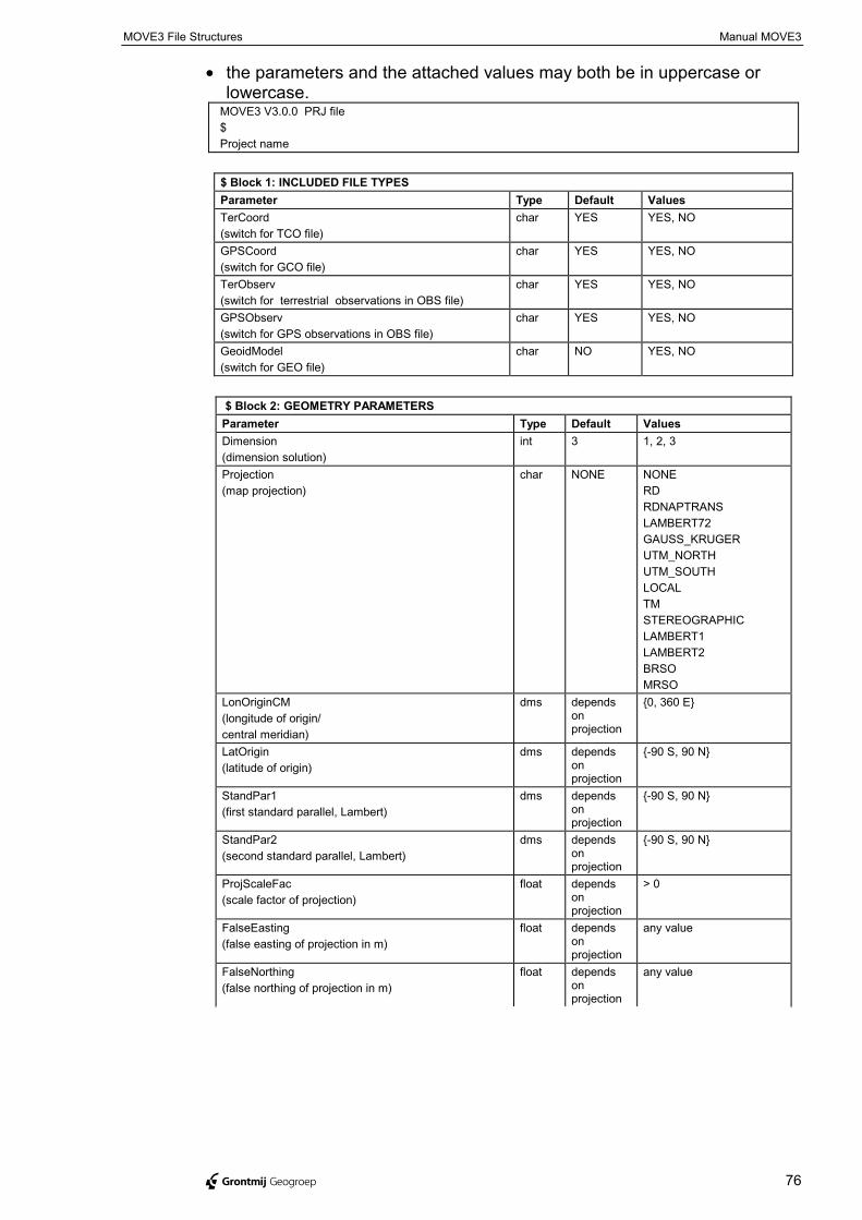
MOVE3 File Structures Manual MOVE3
@ Grontmij Geogroep 76
• the parameters and the attached values may both be in uppercase orlowercase.
MOVE3 V3.0.0 PRJ file $ Project name
$ Block 1: INCLUDED FILE TYPESParameter Type Default ValuesTerCoord(switch for TCO file)
char YES YES, NO
GPSCoord(switch for GCO file)
char YES YES, NO
TerObserv(switch for terrestrial observations in OBS file)
char YES YES, NO
GPSObserv(switch for GPS observations in OBS file)
char YES YES, NO
GeoidModel(switch for GEO file)
char NO YES, NO
$ Block 2: GEOMETRY PARAMETERSParameter Type Default ValuesDimension(dimension solution)
int 3 1, 2, 3
Projection(map projection)
char NONE NONERDRDNAPTRANSLAMBERT72GAUSS_KRUGERUTM_NORTHUTM_SOUTHLOCALTMSTEREOGRAPHICLAMBERT1LAMBERT2BRSOMRSO
LonOriginCM(longitude of origin/central meridian)
dms dependsonprojection
{0, 360 E}
LatOrigin(latitude of origin)
dms dependsonprojection
{-90 S, 90 N}
StandPar1(first standard parallel, Lambert)
dms dependsonprojection
{-90 S, 90 N}
StandPar2(second standard parallel, Lambert)
dms dependsonprojection
{-90 S, 90 N}
ProjScaleFac(scale factor of projection)
float dependsonprojection
> 0
FalseEasting(false easting of projection in m)
float dependsonprojection
any value
FalseNorthing(false northing of projection in m)
float dependsonprojection
any value

MOVE3 File Structures Manual MOVE3
@ Grontmij Geogroep 77
$ Block 2: GEOMETRY PARAMETERSParameter Type Default ValuesEllipsoid(reference ellipsoid)
char to bespecified
USERAIRYMODIFIED_AIRYAUSTRALIAN_NATIONALBESSEL_1841MODIFIED_BESSELCLARKE_1866CLARKE_1880EVERESTMODIFIED_EVERESTFISHER_1960MODIFIED_FISHER_1960FISHER_1968GRS_1967GRS_1980HELMERT_1906HOUGHINTERNATIONALKRASSOVSKY_1940SOUTH_AMERICAN_1969WGS72WGS84TIMBALAI_EVEREST
SemiMajAx(semi major axis reference ellipsoid in m)
float to bespecified
> 0
InvFlatt(inverse flattening reference ellipsoid)
float to bespecified
> 0
TransProj char NONE NONERDNAPTRANS
GPSCoordType(type of GPS coordinates)
char XYZ XYZ, ELL, ENH
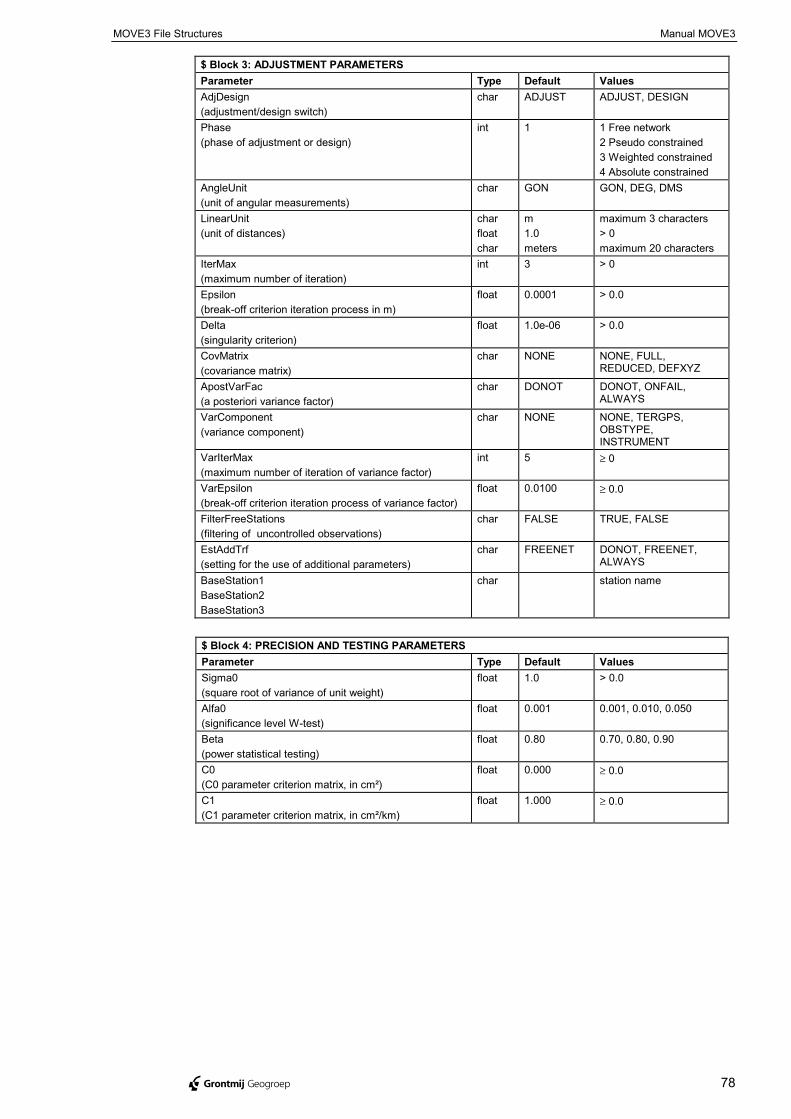
MOVE3 File Structures Manual MOVE3
@ Grontmij Geogroep 78
$ Block 3: ADJUSTMENT PARAMETERSParameter Type Default ValuesAdjDesign(adjustment/design switch)
char ADJUST ADJUST, DESIGN
Phase(phase of adjustment or design)
int 1 1 Free network2 Pseudo constrained3 Weighted constrained4 Absolute constrained
AngleUnit(unit of angular measurements)
char GON GON, DEG, DMS
LinearUnit(unit of distances)
charfloatchar
m1.0meters
maximum 3 characters> 0maximum 20 characters
IterMax(maximum number of iteration)
int 3 > 0
Epsilon(break-off criterion iteration process in m)
float 0.0001 > 0.0
Delta(singularity criterion)
float 1.0e-06 > 0.0
CovMatrix(covariance matrix)
char NONE NONE, FULL,REDUCED, DEFXYZ
ApostVarFac(a posteriori variance factor)
char DONOT DONOT, ONFAIL,ALWAYS
VarComponent(variance component)
char NONE NONE, TERGPS,OBSTYPE,INSTRUMENT
VarIterMax(maximum number of iteration of variance factor)
int 5 ≥ 0
VarEpsilon(break-off criterion iteration process of variance factor)
float 0.0100 ≥ 0.0
FilterFreeStations(filtering of uncontrolled observations)
char FALSE TRUE, FALSE
EstAddTrf(setting for the use of additional parameters)
char FREENET DONOT, FREENET,ALWAYS
BaseStation1BaseStation2BaseStation3
char station name
$ Block 4: PRECISION AND TESTING PARAMETERSParameter Type Default ValuesSigma0(square root of variance of unit weight)
float 1.0 > 0.0
Alfa0(significance level W-test)
float 0.001 0.001, 0.010, 0.050
Beta(power statistical testing)
float 0.80 0.70, 0.80, 0.90
C0(C0 parameter criterion matrix, in cm²)
float 0.000 ≥ 0.0
C1(C1 parameter criterion matrix, in cm²/km)
float 1.000 ≥ 0.0
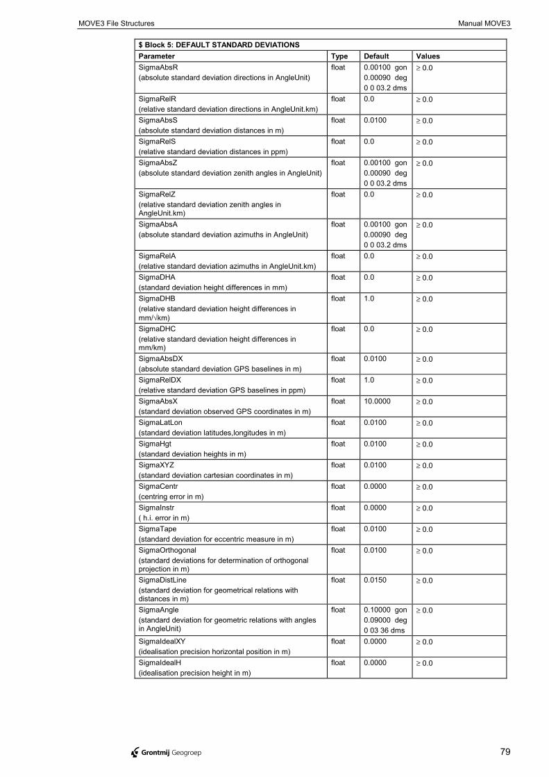
MOVE3 File Structures Manual MOVE3
@ Grontmij Geogroep 79
$ Block 5: DEFAULT STANDARD DEVIATIONSParameter Type Default ValuesSigmaAbsR(absolute standard deviation directions in AngleUnit)
float 0.00100 gon0.00090 deg0 0 03.2 dms
≥ 0.0
SigmaRelR(relative standard deviation directions in AngleUnit.km)
float 0.0 ≥ 0.0
SigmaAbsS(absolute standard deviation distances in m)
float 0.0100 ≥ 0.0
SigmaRelS(relative standard deviation distances in ppm)
float 0.0 ≥ 0.0
SigmaAbsZ(absolute standard deviation zenith angles in AngleUnit)
float 0.00100 gon0.00090 deg0 0 03.2 dms
≥ 0.0
SigmaRelZ(relative standard deviation zenith angles inAngleUnit.km)
float 0.0 ≥ 0.0
SigmaAbsA(absolute standard deviation azimuths in AngleUnit)
float 0.00100 gon0.00090 deg0 0 03.2 dms
≥ 0.0
SigmaRelA(relative standard deviation azimuths in AngleUnit.km)
float 0.0 ≥ 0.0
SigmaDHA(standard deviation height differences in mm)
float 0.0 ≥ 0.0
SigmaDHB(relative standard deviation height differences inmm/√km)
float 1.0 ≥ 0.0
SigmaDHC(relative standard deviation height differences inmm/km)
float 0.0 ≥ 0.0
SigmaAbsDX(absolute standard deviation GPS baselines in m)
float 0.0100 ≥ 0.0
SigmaRelDX(relative standard deviation GPS baselines in ppm)
float 1.0 ≥ 0.0
SigmaAbsX(standard deviation observed GPS coordinates in m)
float 10.0000 ≥ 0.0
SigmaLatLon(standard deviation latitudes,longitudes in m)
float 0.0100 ≥ 0.0
SigmaHgt(standard deviation heights in m)
float 0.0100 ≥ 0.0
SigmaXYZ(standard deviation cartesian coordinates in m)
float 0.0100 ≥ 0.0
SigmaCentr(centring error in m)
float 0.0000 ≥ 0.0
SigmaInstr( h.i. error in m)
float 0.0000 ≥ 0.0
SigmaTape(standard deviation for eccentric measure in m)
float 0.0100 ≥ 0.0
SigmaOrthogonal(standard deviations for determination of orthogonalprojection in m)
float 0.0100 ≥ 0.0
SigmaDistLine(standard deviation for geometrical relations withdistances in m)
float 0.0150 ≥ 0.0
SigmaAngle(standard deviation for geometric relations with anglesin AngleUnit)
float 0.10000 gon0.09000 deg0 03 36 dms
≥ 0.0
SigmaIdealXY(idealisation precision horizontal position in m)
float 0.0000 ≥ 0.0
SigmaIdealH(idealisation precision height in m)
float 0.0000 ≥ 0.0
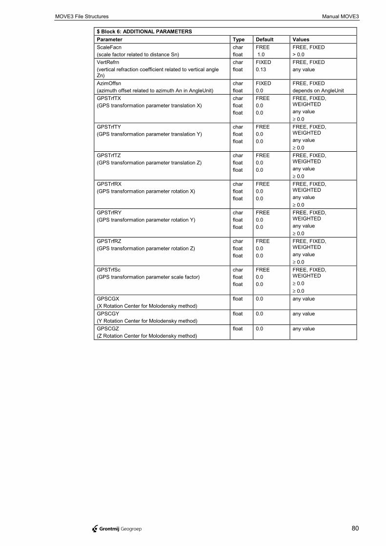
MOVE3 File Structures Manual MOVE3
@ Grontmij Geogroep 80
$ Block 6: ADDITIONAL PARAMETERSParameter Type Default ValuesScaleFacn(scale factor related to distance Sn)
charfloat
FREE 1.0
FREE, FIXED> 0.0
VertRefrn(vertical refraction coefficient related to vertical angleZn)
charfloat
FIXED0.13
FREE, FIXEDany value
AzimOffsn(azimuth offset related to azimuth An in AngleUnit)
charfloat
FIXED0.0
FREE, FIXEDdepends on AngleUnit
GPSTrfTX(GPS transformation parameter translation X)
charfloatfloat
FREE0.00.0
FREE, FIXED,WEIGHTEDany value≥ 0.0
GPSTrfTY(GPS transformation parameter translation Y)
charfloatfloat
FREE0.00.0
FREE, FIXED,WEIGHTEDany value≥ 0.0
GPSTrfTZ(GPS transformation parameter translation Z)
charfloatfloat
FREE0.00.0
FREE, FIXED,WEIGHTEDany value≥ 0.0
GPSTrfRX(GPS transformation parameter rotation X)
charfloatfloat
FREE0.00.0
FREE, FIXED,WEIGHTEDany value≥ 0.0
GPSTrfRY(GPS transformation parameter rotation Y)
charfloatfloat
FREE0.00.0
FREE, FIXED,WEIGHTEDany value≥ 0.0
GPSTrfRZ(GPS transformation parameter rotation Z)
charfloatfloat
FREE0.00.0
FREE, FIXED,WEIGHTEDany value≥ 0.0
GPSTrfSc(GPS transformation parameter scale factor)
charfloatfloat
FREE0.00.0
FREE, FIXED,WEIGHTED≥ 0.0≥ 0.0
GPSCGX(X Rotation Center for Molodensky method)
float 0.0 any value
GPSCGY(Y Rotation Center for Molodensky method)
float 0.0 any value
GPSCGZ(Z Rotation Center for Molodensky method)
float 0.0 any value
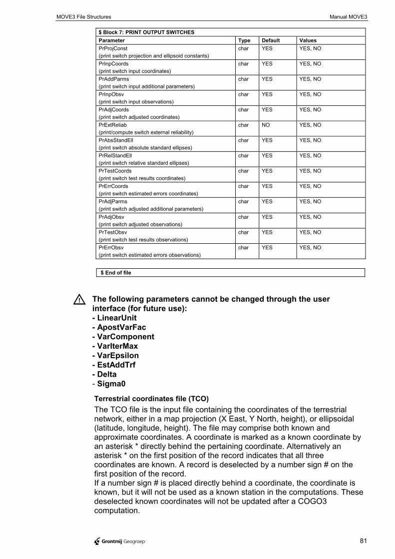
MOVE3 File Structures Manual MOVE3
@ Grontmij Geogroep 81
$ Block 7: PRINT OUTPUT SWITCHESParameter Type Default ValuesPrProjConst(print switch projection and ellipsoid constants)
char YES YES, NO
PrInpCoords(print switch input coordinates)
char YES YES, NO
PrAddParms(print switch input additional parameters)
char YES YES, NO
PrInpObsv(print switch input observations)
char YES YES, NO
PrAdjCoords(print switch adjusted coordinates)
char YES YES, NO
PrExtReliab(print/compute switch external reliability)
char NO YES, NO
PrAbsStandEll(print switch absolute standard ellipses)
char YES YES, NO
PrRelStandEll(print switch relative standard ellipses)
char YES YES, NO
PrTestCoords(print switch test results coordinates)
char YES YES, NO
PrErrCoords(print switch estimated errors coordinates)
char YES YES, NO
PrAdjParms(print switch adjusted additional parameters)
char YES YES, NO
PrAdjObsv(print switch adjusted observations)
char YES YES, NO
PrTestObsv(print switch test results observations)
char YES YES, NO
PrErrObsv(print switch estimated errors observations)
char YES YES, NO
$ End of file
! The following parameters cannot be changed through the userinterface (for future use):- LinearUnit- ApostVarFac- VarComponent- VarIterMax- VarEpsilon- EstAddTrf- Delta- Sigma0
Terrestrial coordinates file (TCO)The TCO file is the input file containing the coordinates of the terrestrialnetwork, either in a map projection (X East, Y North, height), or ellipsoidal(latitude, longitude, height). The file may comprise both known andapproximate coordinates. A coordinate is marked as a known coordinate byan asterisk * directly behind the pertaining coordinate. Alternatively anasterisk * on the first position of the record indicates that all threecoordinates are known. A record is deselected by a number sign # on thefirst position of the record.If a number sign # is placed directly behind a coordinate, the coordinate isknown, but it will not be used as a known station in the computations. Thesedeselected known coordinates will not be updated after a COGO3computation.
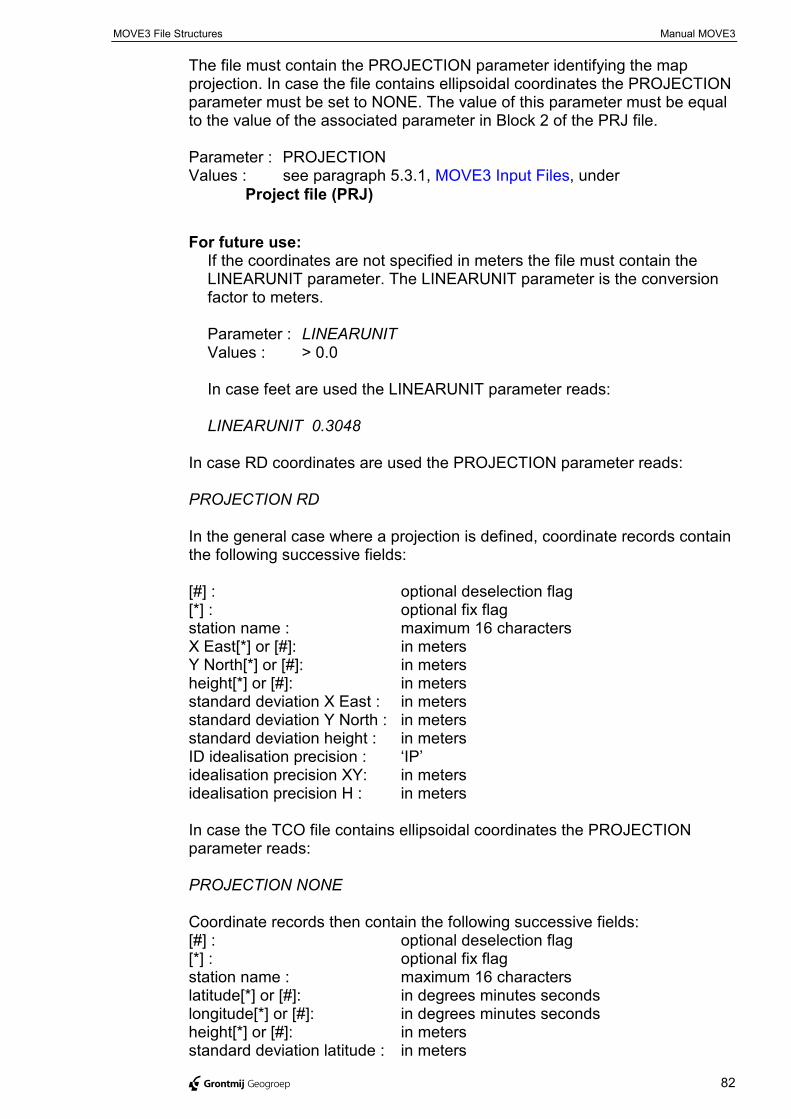
MOVE3 File Structures Manual MOVE3
@ Grontmij Geogroep 82
The file must contain the PROJECTION parameter identifying the mapprojection. In case the file contains ellipsoidal coordinates the PROJECTIONparameter must be set to NONE. The value of this parameter must be equalto the value of the associated parameter in Block 2 of the PRJ file.
Parameter : PROJECTIONValues : see paragraph 5.3.1, MOVE3 Input Files, under
Project file (PRJ)
For future use:If the coordinates are not specified in meters the file must contain theLINEARUNIT parameter. The LINEARUNIT parameter is the conversionfactor to meters.
Parameter : LINEARUNITValues : > 0.0
In case feet are used the LINEARUNIT parameter reads:
LINEARUNIT 0.3048
In case RD coordinates are used the PROJECTION parameter reads:
PROJECTION RD
In the general case where a projection is defined, coordinate records containthe following successive fields:
[#] : optional deselection flag[*] : optional fix flagstation name : maximum 16 charactersX East[*] or [#]: in metersY North[*] or [#]: in metersheight[*] or [#]: in metersstandard deviation X East : in metersstandard deviation Y North : in metersstandard deviation height : in metersID idealisation precision : ‘IP’idealisation precision XY: in metersidealisation precision H : in meters
In case the TCO file contains ellipsoidal coordinates the PROJECTIONparameter reads:
PROJECTION NONE
Coordinate records then contain the following successive fields:[#] : optional deselection flag[*] : optional fix flagstation name : maximum 16 characterslatitude[*] or [#]: in degrees minutes secondslongitude[*] or [#]: in degrees minutes secondsheight[*] or [#]: in metersstandard deviation latitude : in meters
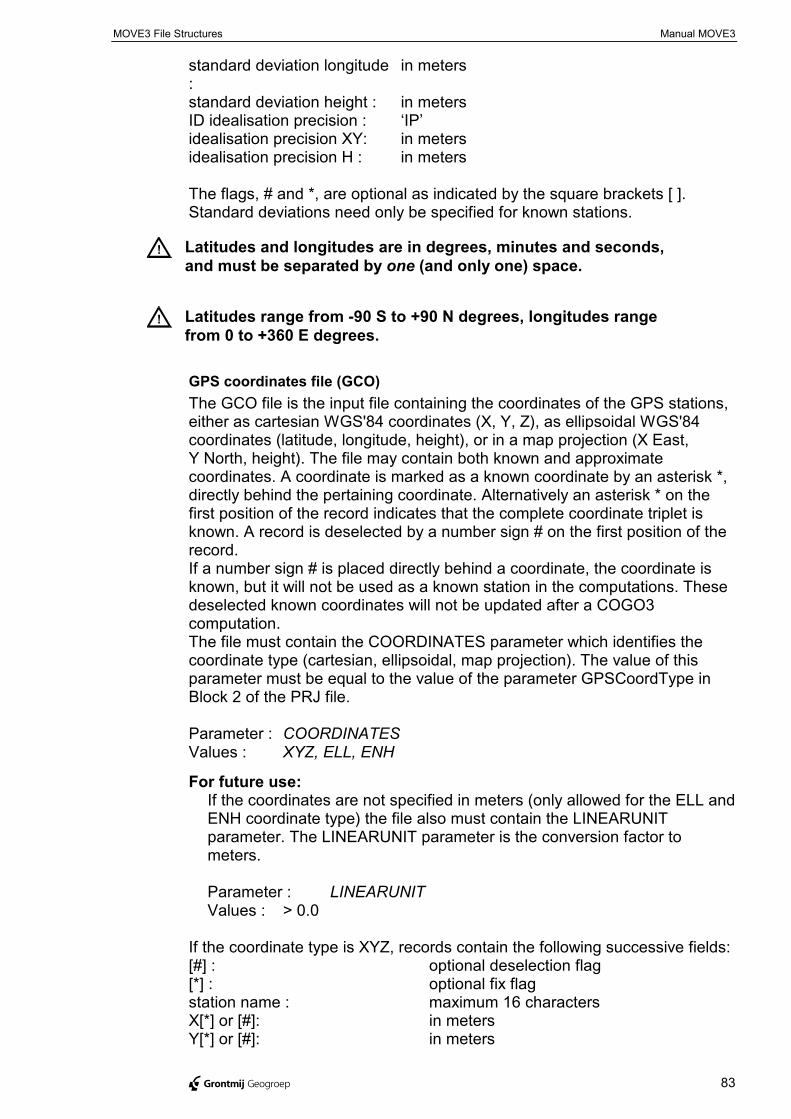
MOVE3 File Structures Manual MOVE3
@ Grontmij Geogroep 83
standard deviation longitude:
in meters
standard deviation height : in metersID idealisation precision : ‘IP’idealisation precision XY: in metersidealisation precision H : in meters
The flags, # and *, are optional as indicated by the square brackets [ ].Standard deviations need only be specified for known stations.
! Latitudes and longitudes are in degrees, minutes and seconds,and must be separated by one (and only one) space.
! Latitudes range from -90 S to +90 N degrees, longitudes rangefrom 0 to +360 E degrees.
GPS coordinates file (GCO)The GCO file is the input file containing the coordinates of the GPS stations,either as cartesian WGS'84 coordinates (X, Y, Z), as ellipsoidal WGS'84coordinates (latitude, longitude, height), or in a map projection (X East,Y North, height). The file may contain both known and approximatecoordinates. A coordinate is marked as a known coordinate by an asterisk *,directly behind the pertaining coordinate. Alternatively an asterisk * on thefirst position of the record indicates that the complete coordinate triplet isknown. A record is deselected by a number sign # on the first position of therecord.If a number sign # is placed directly behind a coordinate, the coordinate isknown, but it will not be used as a known station in the computations. Thesedeselected known coordinates will not be updated after a COGO3computation.The file must contain the COORDINATES parameter which identifies thecoordinate type (cartesian, ellipsoidal, map projection). The value of thisparameter must be equal to the value of the parameter GPSCoordType inBlock 2 of the PRJ file.
Parameter : COORDINATESValues : XYZ, ELL, ENH
For future use:If the coordinates are not specified in meters (only allowed for the ELL andENH coordinate type) the file also must contain the LINEARUNITparameter. The LINEARUNIT parameter is the conversion factor tometers.
Parameter : LINEARUNITValues : > 0.0
If the coordinate type is XYZ, records contain the following successive fields:[#] : optional deselection flag[*] : optional fix flagstation name : maximum 16 charactersX[*] or [#]: in metersY[*] or [#]: in meters
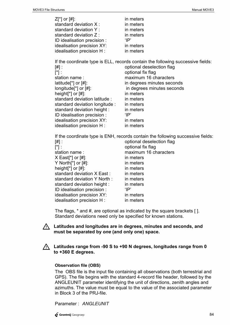
MOVE3 File Structures Manual MOVE3
@ Grontmij Geogroep 84
Z[*] or [#]: in metersstandard deviation X : in metersstandard deviation Y : in metersstandard deviation Z : in metersID idealisation precision : ‘IP’idealisation precision XY: in metersidealisation precision H : in meters
If the coordinate type is ELL, records contain the following successive fields:[#] : optional deselection flag[*] : optional fix flagstation name : maximum 16 characterslatitude[*] or [#]: in degrees minutes secondslongitude[*] or [#]: in degrees minutes secondsheight[*] or [#]: in metersstandard deviation latitude : in metersstandard deviation longitude : in metersstandard deviation height : in metersID idealisation precision : ‘IP’idealisation precision XY: in metersidealisation precision H : in meters
If the coordinate type is ENH, records contain the following successive fields:[#] : optional deselection flag[*] : optional fix flagstation name : maximum 16 charactersX East[*] or [#]: in metersY North[*] or [#]: in metersheight[*] or [#]: in metersstandard deviation X East : in metersstandard deviation Y North : in metersstandard deviation height : in metersID idealisation precision : ‘IP’idealisation precision XY: in metersidealisation precision H : in meters
The flags, * and #, are optional as indicated by the square brackets [ ].Standard deviations need only be specified for known stations.
! Latitudes and longitudes are in degrees, minutes and seconds, andmust be separated by one (and only one) space.
! Latitudes range from -90 S to +90 N degrees, longitudes range from 0to +360 E degrees.
Observation file (OBS)The OBS file is the input file containing all observations (both terrestrial andGPS). The file begins with the standard 4-record file header, followed by theANGLEUNIT parameter identifying the unit of directions, zenith angles andazimuths. The value must be equal to the value of the associated parameterin Block 3 of the PRJ-file.
Parameter : ANGLEUNIT
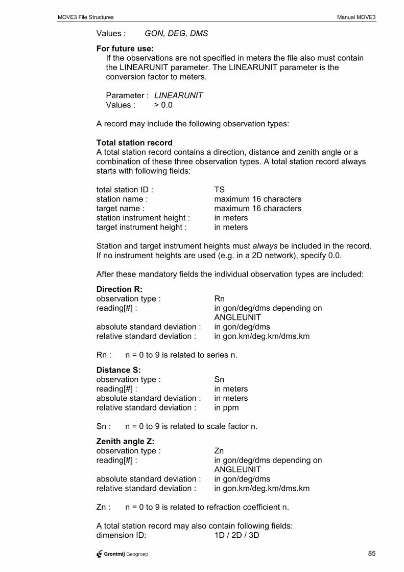
MOVE3 File Structures Manual MOVE3
@ Grontmij Geogroep 85
Values : GON, DEG, DMS
For future use:If the observations are not specified in meters the file also must containthe LINEARUNIT parameter. The LINEARUNIT parameter is theconversion factor to meters.
Parameter : LINEARUNITValues : > 0.0
A record may include the following observation types:
Total station recordA total station record contains a direction, distance and zenith angle or acombination of these three observation types. A total station record alwaysstarts with following fields:
total station ID : TSstation name : maximum 16 characterstarget name : maximum 16 charactersstation instrument height : in meterstarget instrument height : in meters
Station and target instrument heights must always be included in the record.If no instrument heights are used (e.g. in a 2D network), specify 0.0.
After these mandatory fields the individual observation types are included:
Direction R:observation type : Rnreading[#] : in gon/deg/dms depending on
ANGLEUNITabsolute standard deviation : in gon/deg/dmsrelative standard deviation : in gon.km/deg.km/dms.km
Rn : n = 0 to 9 is related to series n.
Distance S:observation type : Snreading[#] : in metersabsolute standard deviation : in metersrelative standard deviation : in ppm
Sn : n = 0 to 9 is related to scale factor n.
Zenith angle Z:observation type : Znreading[#] : in gon/deg/dms depending on
ANGLEUNITabsolute standard deviation : in gon/deg/dmsrelative standard deviation : in gon.km/deg.km/dms.km
Zn : n = 0 to 9 is related to refraction coefficient n.
A total station record may also contain following fields:dimension ID: 1D / 2D / 3D
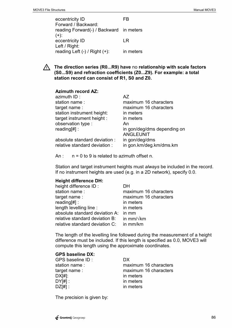
MOVE3 File Structures Manual MOVE3
@ Grontmij Geogroep 86
eccentricity IDForward / Backward:
FB
reading Forward(-) / Backward(+):
in meters
eccentricity IDLeft / Right:
LR
reading Left (-) / Right (+): in meters
! The direction series (R0...R9) have no relationship with scale factors(S0...S9) and refraction coefficients (Z0...Z9). For example: a totalstation record can consist of R1, S0 and Z0.
Azimuth record AZ:azimuth ID : AZstation name : maximum 16 characterstarget name : maximum 16 charactersstation instrument height: in meterstarget instrument height : in metersobservation type : Anreading[#] : in gon/deg/dms depending on
ANGLEUNITabsolute standard deviation : in gon/deg/dmsrelative standard deviation : in gon.km/deg.km/dms.km
An : n = 0 to 9 is related to azimuth offset n.
Station and target instrument heights must always be included in the record.If no instrument heights are used (e.g. in a 2D network), specify 0.0.
Height difference DH:height difference ID : DHstation name : maximum 16 characterstarget name : maximum 16 charactersreading[#] : in meterslength levelling line : in metersabsolute standard deviation A: in mmrelative standard deviation B: in mm/√kmrelative standard deviation C: in mm/km
The length of the levelling line followed during the measurement of a heightdifference must be included. If this length is specified as 0.0, MOVE3 willcompute this length using the approximate coordinates.
GPS baseline DX:GPS baseline ID : DXstation name : maximum 16 characterstarget name : maximum 16 charactersDX[#]: in metersDY[#] : in metersDZ[#] : in meters
The precision is given by:
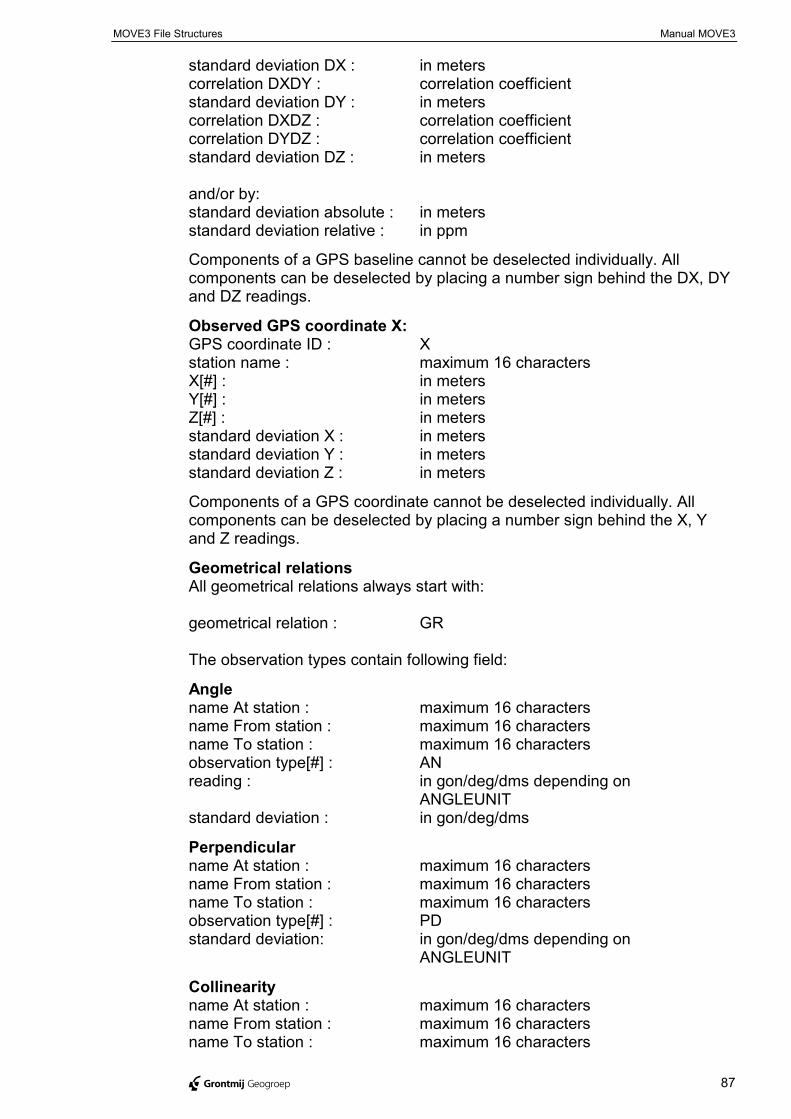
MOVE3 File Structures Manual MOVE3
@ Grontmij Geogroep 87
standard deviation DX : in meterscorrelation DXDY : correlation coefficientstandard deviation DY : in meterscorrelation DXDZ : correlation coefficientcorrelation DYDZ : correlation coefficientstandard deviation DZ : in meters
and/or by:standard deviation absolute : in metersstandard deviation relative : in ppm
Components of a GPS baseline cannot be deselected individually. Allcomponents can be deselected by placing a number sign behind the DX, DYand DZ readings.
Observed GPS coordinate X:GPS coordinate ID : Xstation name : maximum 16 charactersX[#] : in metersY[#] : in metersZ[#] : in metersstandard deviation X : in metersstandard deviation Y : in metersstandard deviation Z : in meters
Components of a GPS coordinate cannot be deselected individually. Allcomponents can be deselected by placing a number sign behind the X, Yand Z readings.
Geometrical relationsAll geometrical relations always start with:
geometrical relation : GR
The observation types contain following field:
Anglename At station : maximum 16 charactersname From station : maximum 16 charactersname To station : maximum 16 charactersobservation type[#] : ANreading : in gon/deg/dms depending on
ANGLEUNITstandard deviation : in gon/deg/dms
Perpendicularname At station : maximum 16 charactersname From station : maximum 16 charactersname To station : maximum 16 charactersobservation type[#] : PDstandard deviation: in gon/deg/dms depending on
ANGLEUNIT
Collinearityname At station : maximum 16 charactersname From station : maximum 16 charactersname To station : maximum 16 characters
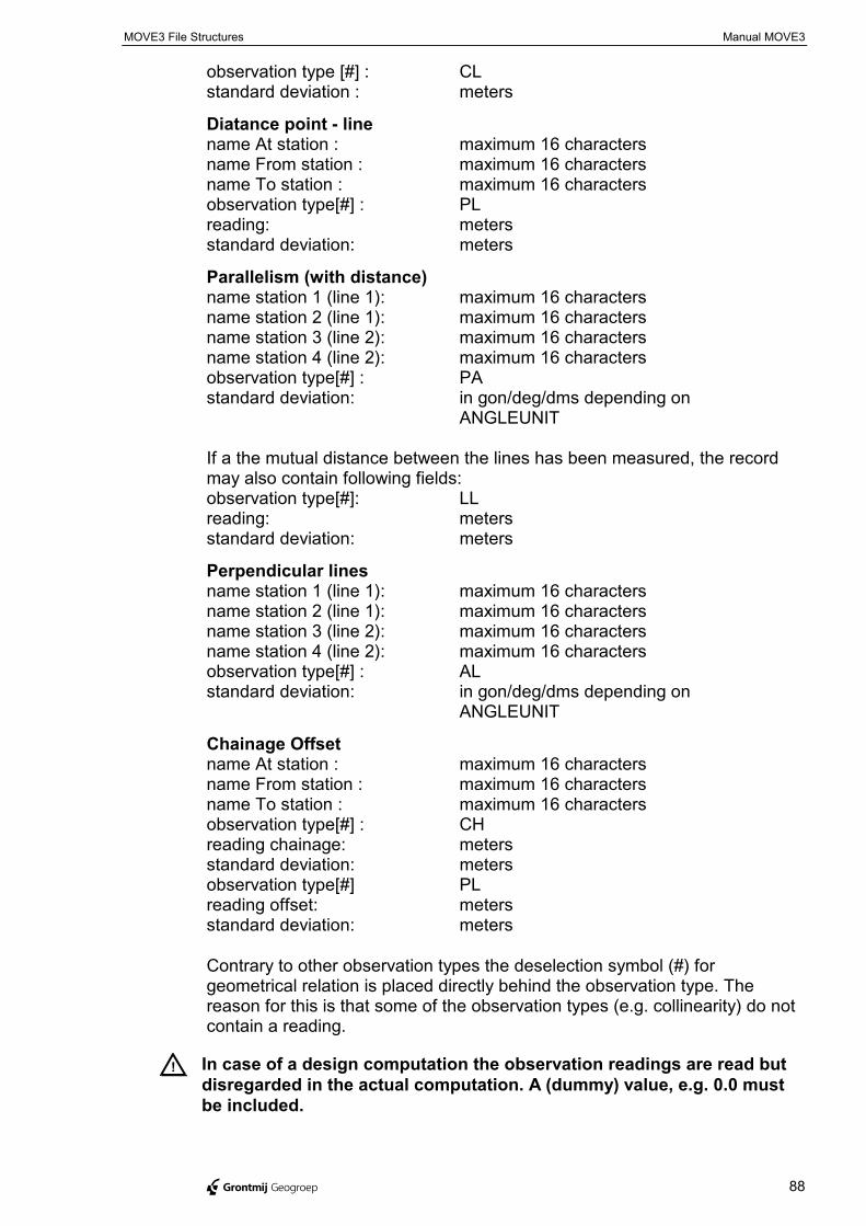
MOVE3 File Structures Manual MOVE3
@ Grontmij Geogroep 88
observation type [#] : CLstandard deviation : meters
Diatance point - linename At station : maximum 16 charactersname From station : maximum 16 charactersname To station : maximum 16 charactersobservation type[#] : PLreading: metersstandard deviation: meters
Parallelism (with distance)name station 1 (line 1): maximum 16 charactersname station 2 (line 1): maximum 16 charactersname station 3 (line 2): maximum 16 charactersname station 4 (line 2): maximum 16 charactersobservation type[#] : PAstandard deviation: in gon/deg/dms depending on
ANGLEUNIT
If a the mutual distance between the lines has been measured, the recordmay also contain following fields:observation type[#]: LLreading: metersstandard deviation: meters
Perpendicular linesname station 1 (line 1): maximum 16 charactersname station 2 (line 1): maximum 16 charactersname station 3 (line 2): maximum 16 charactersname station 4 (line 2): maximum 16 charactersobservation type[#] : ALstandard deviation: in gon/deg/dms depending on
ANGLEUNIT
Chainage Offsetname At station : maximum 16 charactersname From station : maximum 16 charactersname To station : maximum 16 charactersobservation type[#] : CHreading chainage: metersstandard deviation: metersobservation type[#] PLreading offset: metersstandard deviation: meters
Contrary to other observation types the deselection symbol (#) forgeometrical relation is placed directly behind the observation type. Thereason for this is that some of the observation types (e.g. collinearity) do notcontain a reading.
! In case of a design computation the observation readings are read butdisregarded in the actual computation. A (dummy) value, e.g. 0.0 mustbe included.
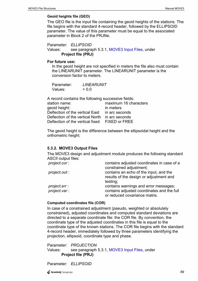
MOVE3 File Structures Manual MOVE3
@ Grontmij Geogroep 89
Geoid heights file (GEO)The GEO file is the input file containing the geoid heights of the stations. Thefile begins with the standard 4-record header, followed by the ELLIPSOIDparameter. The value of this parameter must be equal to the associatedparameter in Block 2 of the PRJfile.
Parameter: ELLIPSOIDValues: see paragraph 5.3.1, MOVE3 Input Files, under
Project file (PRJ)
For future use:In the geoid height are not specified in meters the file also must containthe LINEARUNIT parameter. The LINEARUNIT parameter is theconversion factor to meters.
Parameter: LINEARUNITValues: > 0.0
A record contains the following successive fields:station name: maximum 16 charactersgeoid height: in metersDeflection of the vertical East in arc secondsDeflection of the vertical North in arc secondsDeflection of the vertical fixed FIXED or FREE
The geoid height is the difference between the ellipsoidal height and theorthometric height.
5.3.2. MOVE3 Output FilesThe MOVE3 design and adjustment module produces the following standardASCII output files:project.cor : contains adjusted coordinates in case of a
constrained adjustment;project.out : contains an echo of the input, and the
results of the design or adjustment andtesting;
project.err : contains warnings and error messages;project.var : contains adjusted coordinates and the full
or reduced covariance matrix.
Computed coordinates file (COR)In case of a constrained adjustment (pseudo, weighted or absolutelyconstrained), adjusted coordinates and computed standard deviations aredirected to a separate coordinate file: the COR file. By convention, thecoordinate type of the adjusted coordinates in this file is equal to thecoordinate type of the known stations. The COR file begins with the standard4-record header, immediately followed by three parameters identifying theprojection, ellipsoid, coordinate type and phase.
Parameter: PROJECTIONValues: see paragraph 5.3.1, MOVE3 Input Files, under
Project file (PRJ)
Parameter: ELLIPSOID
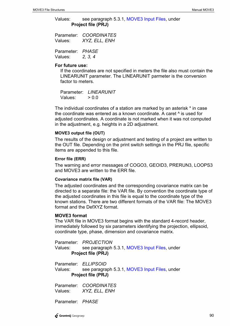
MOVE3 File Structures Manual MOVE3
@ Grontmij Geogroep 90
Values: see paragraph 5.3.1, MOVE3 Input Files, underProject file (PRJ)
Parameter: COORDINATESValues: XYZ, ELL, ENH
Parameter: PHASEValues: 2, 3, 4
For future use:If the coordinates are not specified in meters the file also must contain theLINEARUNIT parameter. The LINEARUNIT parmeter is the conversionfactor to meters.
Parameter: LINEARUNITValues: > 0.0
The individual coordinates of a station are marked by an asterisk * in casethe coordinate was entered as a known coordinate. A caret ^ is used foradjusted coordinates. A coordinate is not marked when it was not computedin the adjustment, e.g. heights in a 2D adjustment.
MOVE3 output file (OUT)The results of the design or adjustment and testing of a project are written tothe OUT file. Depending on the print switch settings in the PRJ file, specificitems are appended to this file.
Error file (ERR)The warning and error messages of COGO3, GEOID3, PRERUN3, LOOPS3and MOVE3 are written to the ERR file.
Covariance matrix file (VAR)The adjusted coordinates and the corresponding covariance matrix can bedirected to a separate file: the VAR file. By convention the coordinate type ofthe adjusted coordinates in this file is equal to the coordinate type of theknown stations. There are two different formats of the VAR file: The MOVE3format and the DefXYZ format.
MOVE3 formatThe VAR file in MOVE3 format begins with the standard 4-record header,immediately followed by six parameters identifying the projection, ellipsoid,coordinate type, phase, dimension and covariance matrix.
Parameter: PROJECTIONValues: see paragraph 5.3.1, MOVE3 Input Files, under
Project file (PRJ)
Parameter: ELLIPSOIDValues: see paragraph 5.3.1, MOVE3 Input Files, under
Project file (PRJ)
Parameter: COORDINATESValues: XYZ, ELL, ENH
Parameter: PHASE

MOVE3 File Structures Manual MOVE3
@ Grontmij Geogroep 91
Values: 2, 3, 4
Parameter: DIMENSIONValues: 1, 2, 3
Parameter: COVMATRIXValues: NONE, FULL, REDUCED
For future use:If the coordinates are not specified in meters the file also must contain theLINEARUNIT parameter. The LINEARUNIT parameter is the conversionfactor to meters.
Parameter: LINEARUNITValues: > 0.0
DefXYZ (MD) formatThe VAR file in DefXYZ format begins with one headerline containing thePRJ file name, date, number of stations, dimension and phase.
Manual MOVE3
@ Grontmij Geogroep 92
5.4. GlossaryAzimuth: The angle between the North direction and the direction to a
target.Base stations: The base stations are the stations to which the network is
connected in a free network adjustment. By fixing the minimum numberof coordinates (i.e. without extra constraints) only location, orientationand scale of the network is defined.
Baseline: A three-dimensional vector in WGS'84 between two stations.Bias to Noise Ratio (BNR): The BNR gives the influence of a possible
outlier (size MDB) in an observation on all coordinates. The BNR isregarded as the ratio between reliability and precision.
Cartesian coordinate system: An orthonormal coordinate system, with thesame scale on all axes, with coordinates taken as segments on the axesdenoted by, in case of a three dimensional system, (X,Y,Z).
Collinearity: The geometrical relation that three points are located on astraight line.
Constrained adjustment: In a constrained adjustment the network isconnected to all known stations. MOVE3 discriminates between threetypes of constrained adjustments. In a pseudo constrained adjustmentthe known coordinates do not get corrections, and the standarddeviations of the known stations do not change. In a weightedconstrained adjustment the known coordinates are considered asnormal observations and they will get corrections in the adjustment. In anabsolutely constrained adjustment the known coordinates do not getcorrections and the standard deviations of the known stations will be 0after the adjustment.
Correlation: There is correlation between two quantities when thesequantities are statistically dependent, i.e. the quantities influence eachother. Correlation is expressed by ρ, the correlation coefficient.
Criterion circle: The criterion circles determine a theoretical modelrepresenting a homogeneous precision, with respect to the basestations. Criterion circles are used when judging the standard ellipses(which depend on the choice of the base stations) in a free networkadjustment.
Critical value: The predetermined value, which decides over acceptance orrejection of a hypothesis, associated with a statistical test.
Datasnooping: Statistical testing method in which every observation istested separately by the W-test.
Datum: A mathematical model, the ellipsoid, designed to best fit the earth'ssurface as a whole or over a certain region. It is defined by giving theellipsoidal parameters (semi major axis, flattening) and the parameters tofix the position of the ellipsoid.
Degree of freedom: see redundancy.
Glossary Manual MOVE3
@ Grontmij Geogroep 93
Design: When designing a network the configuration, consisting of knownand unknown stations and the observations between them, isestablished before realization in the field. The quality of the networkdesign can be rated in terms of precision and reliability.
Distance: The length of the vector between two stations. The slope distancerepresents the directly measured distance from instrument to reflector,while the horizontal distance represents the distance after reduction.
Eccentricity (e): One of the parameters defining the geometry of anellipsoid:
e² = f (2 - f) = (a² - b²)/a²with
f = flattening;a = semi major axis;b = semi minor axis.
(See also flattening f.)Ellipsoid: A mathematical figure formed by revolving an ellipse about its
semi minor axis b. An ellipsoid is usually defined by its semi major axis aand by its flattening, f = (a - b)/a.
Ellipsoid height (h): The vertical distance to a mark above the ellipsoid.
Expectation value (µµµµ): The expectation value of a stochastic variable is theweighted mean value over all possible outcomes of the measurementprocess.
External Reliability: The maximum influence of an error of the size of theMDB on the final coordinate.
F-test: Overall model test, which is used to check the null-hypothesis.Flattening (f): One of the parameters defining the geometry of an ellipsoid:
f = (a - b)/awith
a = semi major axis;b = semi minor axis.
Free network adjustment: Adjustment in which the location, orientation andscale of the network are defined by imposing a minimum number ofconstraints (i.e. by fixing only the base stations). A free networkadjustment is used to test the observations before connecting thenetwork to all known stations.
Geometrical relations: Collection of observation types: angle, perpendicular(3 points or 2 lines), collinearity, distance between point and line,parallelism and chanaige and offset.
Geoid: The gravity equipotential surface, which best approximates the meansea level over the whole earth. The geoid serves as vertical datum fororthometric heights.
Geoid height (N): The difference between ellipsoidal height and orthometricheight: N = h - H.
Glossary Manual MOVE3
@ Grontmij Geogroep 94
GPS: Global Positioning System, a satellite-based system for determiningthree-dimensional relative and absolute positions.
Hypothesis: Set of assumptions on the behaviour of stochastic variables. Aspecial hypothesis is the null-hypothesis H0 that implies the correctnessof the stochastic and mathematical model and the absence of grosserrors in the observations. Statistical testing is used to verify hypotheses.
Known station: A known station is a station of which coordinates are givenwith a certain precision prior to the adjustment. A network is connectedto the known stations in a constrained adjustment.
Least squares adjustment: A method for obtaining unknowns fromredundant observations based on the least squares criterion. Theunknowns are related to the observations by the mathematical model.The least squares criterion says that the sum of squares of thecorrections to the observations must be minimal. The least squarescorrections are also known as residuals.
Map projection: Set of mathematical formulae, which transfers ellipsoidalcoordinates (latitude and longitude) into plane coordinates (X East, YNorth), and vice versa. The transformation results in distortion ofgeometric elements, distance and angle. The most commonly used mapprojections in geodesy are Transverse Mercator, Lambert andStereographic projection.
Mathematical model: A model, which expresses the relationship betweenthe observations and the unknowns in an adjustment.
Minimal Detectable Bias (MDB): The smallest outlier in an observation or aknown coordinate, which can be detected by the W-test with a certainprobability. This probability is equal to the power of the statistical testing.
Minimal Detectable Bias, normalised (MDBn): Describes the internalreliability of the network. For uncorrelated observations equal to the MDBdivided by the standard deviation of the observation.
Observation: An observation is the realisation of a stochastic variable.Orientation: The orientation is the reference direction of the theodolite. For
each station where directions are observed, an orientation unknown issolved in the adjustment. Each extra measurement series results in anextra orientation unknown.
Orthometric height (H): The vertical distance to a mark above the geoid.Vertical here means: along the direction of the local force of gravity.
Phase adjustment: An adjustment can be subdivided into phases; a freenetwork adjustment and a constrained adjustment. The latter can besubdivided in a pseudo constrained adjustment, weighted constrainedadjustment or an absolutely constrained adjustment.
Positioning: The determination of the coordinates of a station with respectto a well-defined coordinate system. By relative positioning coordinatedifferences are determined rather than absolute coordinates.
Precision: Precision represents the stochastic deviations in observationsand coordinates. Precision is quantified by standard deviations andstandard ellipses.
Glossary Manual MOVE3
@ Grontmij Geogroep 95
Probability: Probability is related to the frequency of occurrence of a specificoutcome of the measurement process. Each outcome has an associatedprobability. The probability distribution describes the probabilities asrelated to the possible outcomes of a stochastic variable.
Pseudo least squares adjustment: Adjustment to connect the network toall known stations without corrections to the known coordinates.
Redundancy: The redundancy, also called the degree of freedom, in anadjustment is equal to the number of observations minus the number ofunknowns.
Redundancy number: The (local) redundancy number presents thecontribution of an observation to the total redundancy. The sum of thelocal redundancy numbers equals the degree of freedom.
Refraction coefficient: The influence of the refraction causes a curvature oflight beams in vertical direction. This curvature can be modelled by arefraction coefficient k. Under normal circumstances:
k ≈ 0.13The coefficient has a positive value if the beam is convex (curvaturetowards the earth), and a negative value if the beam is concave(curvature away from the earth).
Reliability: Reliability is the sensitivity of a network configuration to thedetection of outliers. Reliability is quantified by Minimal DetectableBiases, Bias to Noise Ratios and External Reliability.
Singularity: Singularity occurs when one or more unknowns cannot besolved in the adjustment.
Standard deviation (σσσσ): The standard deviation is the standardised measureof precision.
Standard ellipse: The precision of stations in a network is expressed byabsolute standard ellipses. Relative standard ellipses represent theprecision of coordinate differences between two stations. Standardellipses are the 2D equivalent of standard deviations.
Stochastic model: Model, which describes the stochastic deviations of theobservations and known coordinates in an adjustment.
Stochastic variable: A stochastic variable is a variable, which exhibitsrandom or stochastic variabilities. Such a variable can not be describedby a single and exact value, but is usually described by an expectationvalue and a standard deviation.
Terrestrial Observations: Terrestrial observations are observationsobtained without involvement of satellites, e.g. directions, distances,zenith angles, azimuths, and height differences.
T-test: Statistical test used to trace an error in an observation or coordinatepair or triplet. Depending on whether a pair or triplet is tested, the test istwo- or three-dimensional.
Variance (σσσσ²): The variance is the square of the standard deviation.Variance Component Analysis: The Variance Component Analysis
provides a separate estimation of the a-posteriori variances for differentobservation types and for different groups of observations of the sametype.

Glossary Manual MOVE3
@ Grontmij Geogroep 96
W-test (datasnooping): One-dimensional statistical test used to traceerroneous observations by testing so-called conventional alternativehypotheses. A conventional alternative hypothesis assumes an outlier inone single observation while the other observations are correct.
WGS'84: World Geodetic System 1984; the global reference system for GPSobservations since January 1987. In some cases its predecessor,WGS'72, is still utilised.
Zenith angle: The vertical angle between the direction to the zenith of theobserver and the direction to a target. The zenith is the direction oppositeto the local direction of the force of gravity.

Index Manual MOVE3
@ Grontmij Geogroep 97
IndexAdjustment 51; 55
absolutely constrained 60constrained 59free network 59pseudo constrained 59weighted constrained 59
Antenna height error 70Azimuths 23; 24Base station 59B-method of testing 68; 70BNR 65Capacity 7Central Meridian 40Constraint 57Conventional alternative hypothesis69Coordinate
approximate 56known 27
Coordinate typecartesian 27; 33ellipsoidal 27; 32projection 27relation with file type 27relation with network type 27
Correction, least squares 55Correlation 58Covariance 58Criterion circle 64Critical value 67Datasnooping 68; 69Datum 33Datum transformation 36Delft Method 51Design 52Dimension switch 25Direction 22Distance 23
horizontal 25slope 25
Ellipsoid 32Estimated error 72False Easting 40; 41; 42False Northing 40; 41; 42File
COR 95ERR 95GCO 27; 88GEO 94OBS 90OUT 95PRJ 80TCO 27; 86VAR 96
Flattening 33Free observation 64
F-test 68Geoid 35Geoid height 35Geoid model 20Geometrical relation 24; 46
angle 24; 46chainage offset 24; 47collinearity 24; 47distance point - line 24; 47parallelism 24; 47perpendicular 24; 46perpendicular lines 24; 47
GPS 43GPS baseline 24GPS coordinate 24Hardware lock 9Height
ellipsoidal 35orthometric 35
Height difference 23trigonometric 26
Hypothesis 67Installation 9Iteration 56Latitude of Origin 40; 41Level of significance 67Longitude of Origin 40; 41Map projection 38MDB 64Mean 57Model
mathematical 20; 55stochastic 57
Nuisance parameter 56Null-hypothesis 67Observation type 22
combining 21; 26relation with dimension 25
Power 67Precision 52; 58; 63Precision of idealisation 48Projection 38
Lambert 40Local (Stereographic) 42Stereographic 40; 41Transverse Mercator 40
Quality 52Redundancy Number 65Reference system
global 33local 33
Reliability 52; 64external 65internal 64
Reliability box 65

Index Manual MOVE3
@ Grontmij Geogroep 98
Requirementshardware 9software 9system 7
Residual 55Scale Factor (projection) 40; 41Semi major axis 33Semi minor axis 33Singularity 57Standard deviation 57; 63Standard ellips 63
absolute 63relative 63
Standard Parallel 41Testing 52Total station record 23T-test 70Variance 58Variance-covariance matrix 59WGS'84 33W-test 69Zenith angle 23