manual of weighing applications - analytical … · manual of weighing applications part 2 ... the...

Manual of Weighing Applications

Part 2

Counting

www.balances.com is your scource from Sartorius at discount prices.

Preface

In many everyday areas of operation, the scale or the weight is only a means to an end: the quan-tity that is actually of interest is first calculated from the weight or the mass. Therefore, this weig-hing applications handbook covers the most important applications in individual parts, each ofwhich is dedicated to a particular topic.

Counting with the help of scales is the subject of Part 2 of the handbook, which was recently com-pleted. The most important question that arises from the counting application undoubtedly con-cerns the attainable degree of accuracy – or, conversely, the quantity of the unavoidable countingerror.

Four tables in the chapter entitled “Selecting the “Right” Counting Scale” (beginning on p. 20)provide a quick overview of the counting error that can be reached (or falls short of being re-ached) under certain conditions.

The error can be precisely calculated for each individual case using a simple spreadsheet in theEXCEL file “ACCURACY.XLS,” which is included with this handbook.

The fundamentals for determining piece counts based on weights are explained in the handbook.In addition, it illustrates which quantities determine the counting error and how. Some statisticalfundamentals, which provide a better understanding of the counting procedure and of error calcu-lation, are presented at the beginning of the counting applications handbook.

The goal of this handbook is to provide sartorius employees and interested clients with a compre-hensive compilation of information related to the most important weighing applications – for useboth as a training guide in a particular subject area and as a reference. In addition, it will supp-lement or update the user’s knowledge of the subject.

Experiences from cooperation with users in laboratories and industry should give the weighingapplications handbook an “interactive” feeling and enable its continued development through userinput – in the form of short application reports, among other things. With time, these reports willsupplement the handbook and make new and interesting applications available to everyone.

Marketing, Weighing InstrumentsOctober 1999


Meaning of SymbolsMeaning of Symbols

IndicesIndicesrefref related to the reference

number or referenceweight

xx quantity sought

(1)(1) related to 1(representative) part

ii general notation forconsecutive numbering ofindividual values

1, 2, …1, 2, … consecutive numbering ofindividual measuredvalues or parts

SymbolSymbol QuantityQuantityWW weight

Wpronounced:

W bar

mean value of the weights

xx any measured value

xpronounced:

x bar

mean value

∆∆xx scatter of the individualvalues

∆x scatter of the mean value

nn number of measurementsor individual parts

ss standard deviation

ss22 variance

sx

coefficient of variation,relative standarddeviation

tt statistical factor,STUDENT factor

PP confidence interval


2 BK - Oct. 99

Contents:

Counting – a Brief Overview...................................................................................................3

General Fundamentals ............................................................................................................4

Examples for Use of “Counting Scales”...........................................................................................4

Determining the Piece Count Based on the Weight ...........................................................................4

Fundamentals of Statistics.............................................................................................................5Mean Value ...........................................................................................................................5The Meaning of Standard Deviation and Confidence Interval ..........................................................6

Calculating the Counting Error ..............................................................................................11

Piece Count Error .....................................................................................................................11

Comparison of Various Influence Quantities on Counting Accuracy....................................................11

Determining the Counting Accuracy .............................................................................................14

Reference Sample Updating for Optimization........................................................................16

Selecting the “Right” Counting Scale.....................................................................................18

Determining the Suitable Readability of a Scale..............................................................................18

Removal of Reference Samples .............................................................................................24

Appendix..............................................................................................................................26

t Factor or Student Factor for Calculating the Ranges of Dispersion (Scatter).........................................27

Graphs Determining the Counting Accuracy ..................................................................................28

Calculating the Counting Accuracy – Examples of Printouts from the EXCEL File .....................................42

Questions about Counting.....................................................................................................45

Answers to the Questions......................................................................................................46

Register ................................................................................................................................48


3 BK - Oct. 99

Counting – a Brief Overview

Information that is actually of interest to the user is often first calculated from values that were mea-sured using scales. Counting is a weighing application that is used in all areas that depend onquick and reliable determination of the number of individual pieces in a large quantity of equalparts.

The principle behind counting is very simple: the mean value of the individual average pieceweight is calculated based on the weight of a small number of individual parts (the reference piececount). The weight of a large quantity of the same individual parts (the total weight) then onlyneeds to be measured and divided by this mean value to determine the piece count of the weighedquantity. Today, software installed on scales automatically converts the weight into a piece count.The user only needs to perform two weighing operations and enter the number of referencesamples into the scale’s program.

The most important question that arises when counting by weighing relates to the reliability ofthe piece count result: “ Are there really 1,000 screws on the scale as shown in the display, orcould it be only 998, or maybe even 1,005?“

It isn’t necessary to recount 1,000 (or ???) parts to obtain the answer; the error of the counting re-sult can be calculated.

The counting error is influenced by numerous quantities, and the relationships are complex.• The total error is influenced to the greatest extent by the uniformity of the weights of the indivi-

dual parts. This means that the smaller the ever-present (minimal) weight differences are frompiece to piece, the “more accurate” is the resulting total piece count calculated by the scale.This statistical variance of the average piece weight is described mathematically by the stan-dard deviation of the individual parts. The differences in the weights of the individual partsnormally result from manufacture and cannot be readily influenced. The attainable degree ofaccuracy is basically limited by the variance of the individual average piece weights – inde-pendent of the “counting scale” used.

• Of course, the total error of the counting result is influenced by the type of scale selected – theresolution of the scale used to determine the reference weight is of crucial significance here.Comparatively, the resolution of the scale is of lesser importance when determining the totalweight or the total piece count. The resolution of the scale – or the smallest display digit -– mustalways be selected in suitable proportion to the individual piece weight.

• The counting error can be minimized by using larger reference piece counts; for this purpose,Sartorius scales feature a so-called reference optimization function. By gradually increasingthe reference piece count in defined increments, this feature optimizes the basis of calculationused to determine the piece count so that it closely approximates the actual conditions of theweight variance of the individual parts.

Determining large piece counts using scales is a quick and easy counting method. Selecting asuitable scale and using an appropriate piece count leads to optimum results – on the basis ofthe limits set by the variances of the weights of the individual parts.


4 BK - Oct. 99

General Fundamentals

Examples for Use of “Counting Scales”

Counting is the most frequently used weighing application today. It is used extensively in the mostdiverse areas, such as:• incoming inspection• manufacturing• warehousing• packing, and• shipping.

Counting also finds usage in all industrial branches, such as:• precision engineering• the electronics and electrotechnical industries• the plastics industry• paper manufacturing• button manufacturing• in print shops and in book and magazine publishing houses• … .

Determining the Piece Count Based on the Weight

The basic principle behind counting using a scale or by weighing is very simple: if the parts to becounted all have the same weight, the number of individual parts , can be determined by dividingthe combined weight of all parts by the weight of an individual part:

piece countweight of all parts

weight of an individual part=

or n WWx

x

(1)

= . ( 1)

In the process, the average weight of an individual part is first determined by weighing a small,hand-counted number of individual parts – the so-called reference sample quantity:

WWn(1)

ref

ref

= . ( 2)

The equation used for counting with the scale – depending on the weight of the parts to be coun-ted Wx (also referred to as the total weight), the weight of the reference samples Wref and thenumber of reference samples nref – is as follows:

n WnWx x

ref

ref

= ⋅ ( 3)

In reality, the mass of an individual part varies from piece to piece. Therefore, the determinationof the piece count is subject to a statistical error. This means that once a certain number of parts is


5 BK - Oct. 99

reached, the range of error for counting by weighing becomes so large that the accuracy of thepiece count down to one part can no longer be ensured. If the calculated piece count deviates byexactly ± 0.5 from a whole number (e.g., 100.5), it is uncertain whether the piece count is actual-ly 100 or 101.

The more the individual weights of the parts to be counted vary from their mean value, the larger isthe error that can occur while determining the piece count.

The following sections will briefly illustrate the fundamentals of statistics – as far as they arenecessary for understanding counting accuracy. Examples will be given and figures will be presen-ted for calculating the counting error under various conditions.

Finally, systematic errors that can occur while determining the piece count based on the weights ofthe parts will be explained. These errors are often greater than statistical or random errors but canlargely be avoided by adhering to standard operating procedures (see p. 24, Sampling while de-termining the reference weight), while, in general, statistical errors always occur.

Fundamentals of Statistics

In statistics, inferences as to the population are made on the basis of information gathered fromsmall, random samples with the help of applicable mathematical models. The most important quan-tities for characterizing, for example, the uniformity of the weight (mass) of “identical” parts are themean value and the standard deviation.

Mean Value

The mean value W (read as “W bar”) of a larger number of “equal” parts is calculated from thesum of the individual weights W1 through Wn, divided by the number n of individual weights.Generally speaking, the mean value x of a series of weight measurements is expressed as fol-lows:

x 1n

xii 1

n

= ⋅=∑ . ( 4)

or, applied to the example below where six (n = 6) individual weighing operations W1 throughW6 were performed:

W W W W W W W6

1 2 3 4 5 6=+ + + + +

( 5)

Two different series of weight measurements with “the same” mean value should be considered:


6 BK - Oct. 99

WeightWeight Weighing SWeighing Se-e-ries 1ries 1

Weighing SWeighing Se-e-ries 2ries 2

1 6 g 9.999 g2 8 g 9.998 g3 14 g 10.002 g4 12 g 10.000 g5 15 g 10.001 g6 5 g 10.000 g

In the example above, the mean value of both weighing series is:



Number of individual measure-ments n

6 6

Sum of the individual results 60 g 60.000 g

Mean value W 10 g 10.000 g

By itself, the mean value derived from a series of individual weight measurements provides no in-formation about the accuracy, reproducibility, scatter, or reliability of the measurements or of theparts being weighed. The greater the number of individual weight measurements n is, the betterthe mean value of these few weights describes the “true value” of all underlying weights.

When applied to the task of counting, this means that the mean value calculated while determiningthe average piece weight of a large number of individual parts – a large reference piece count – is“more accurate.” In other words, the total distribution is described more precisely and, therefore,the counting result becomes more exact.

The Meaning of Standard Deviation and Confidence Interval

The standard deviation is the quantity that provides the most important information for statisticalevaluation of a series of weight measurements. The scatter of the individual values is calculatedfrom the standard deviation with the help of statistical factors, e.g., for a specified confidence in-terval of 99 %.

The standard deviation is calculated according to this general formula1 :

( )s 1n 1

x xii 1

n 2

=−

⋅ −=∑ . ( 6)

or – applied to the example where n = 6

s(W W) (W W) (W W) +(W W) +(W W) +(W W)

6 -11

22

23

24

25

26

2

=− + − + − − − −

( 7)

1 Function for calculating the standard deviation according to equation (6) in EXCEL: STABW(...)


7 BK - Oct. 99

The relative standard deviation, i.e., the standard deviation related to the mean value s

W of the

series of weight measurements, is often indicated in percent.

In some cases, references are made to the variance, which is indicated by the value s2. However,this value has no other meaning than the standard deviation s itself.

(Sometimes, for example in OIML2 R 76, an approximation of the standard deviation is also givenfor a series consisting of 6 individual weight measurements: the difference between the maximum

value and the minimum value is divided by 3: s x x3

max min=−

, when n = 6.)



Standard deviation s 4.24 g 0.00141 g

Relative standard dev. s

W in %

42 % 0.014 %

Approximation of the standard de-viation in %

33 % 0.013 %

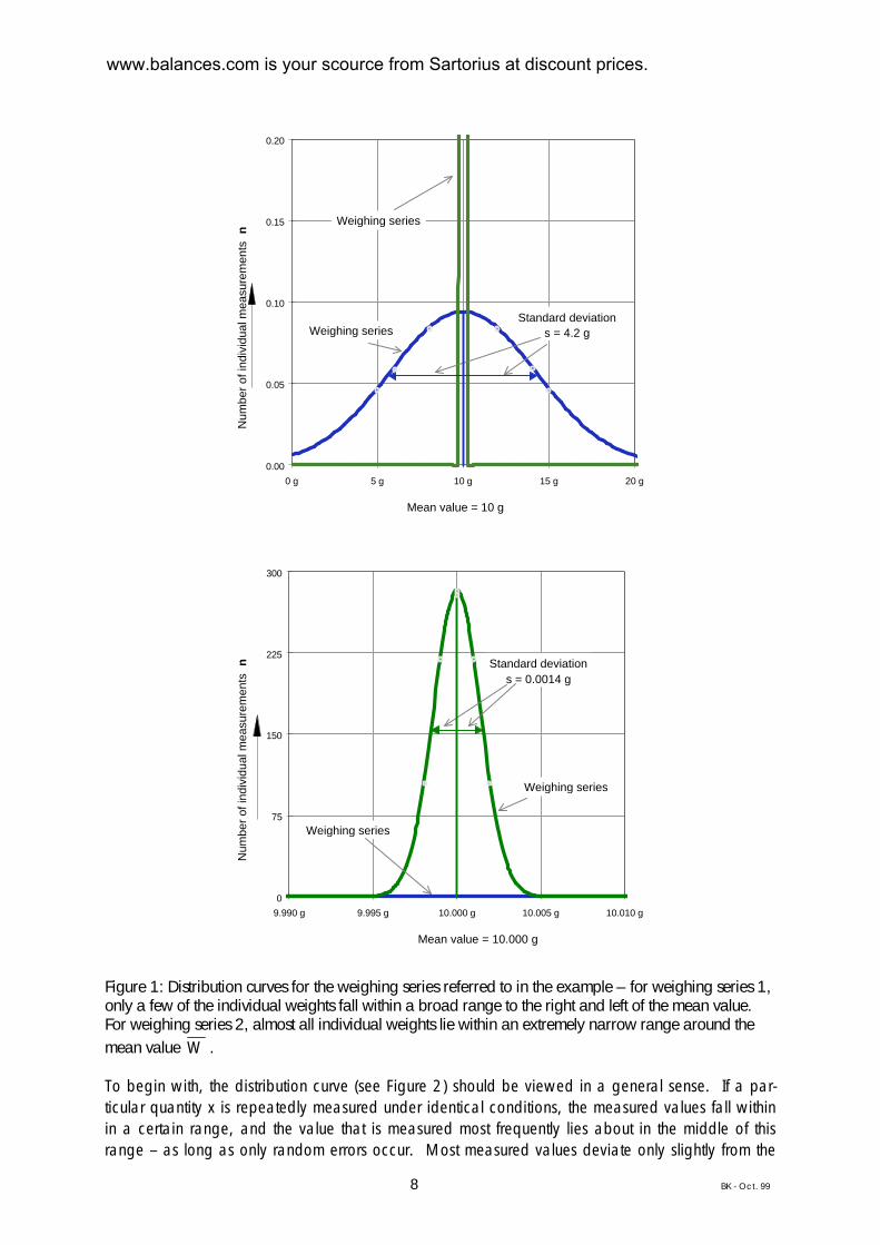
The following figure shows both of the weighing series referred to in the example. These twoweighing series are so different – despite their “shared” mean value of 10 g or 10.000 g – thatthey cannot be presented in one graph. The six individual weights are marked on the curve bycircles. From these few individual weights, an infinitely large number of values is inferred, whichare presented in a bell curve.

2 Organisation Internationale de Métrologie Légale


8 BK - Oct. 99

Figure 1: Distribution curves for the weighing series referred to in the example – for weighing series 1,only a few of the individual weights fall within a broad range to the right and left of the mean value.For weighing series 2, almost all individual weights lie within an extremely narrow range around themean value W .

To begin with, the distribution curve (see Figure 2) should be viewed in a general sense. If a par-ticular quantity x is repeatedly measured under identical conditions, the measured values fall withinin a certain range, and the value that is measured most frequently lies about in the middle of thisrange – as long as only random errors occur. Most measured values deviate only slightly from the

0.00

0.05

0.10

0.15

0.20

0 g 5 g 10 g 15 g 20 g

Num

ber

of in

divi

dual

mea

sure

men

ts

n

Mean value = 10 g

Standard deviations = 4.2 g

Weighing series

Weighing series

0

75

150

225

300

9.990 g 9.995 g 10.000 g 10.005 g 10.010 g

Num

ber

of in

divi

dual

mea

sure

men

ts

n

Mean value = 10.000 g

Standard deviations = 0.0014 g

Weighing series

Weighing series


9 BK - Oct. 99

value most frequently measured, and large deviations from the middle of the range are rare. If thefrequency n, with which the individual measured values occur, is plotted against the measured va-lue x, a distribution curve results. If the number of measurements is very large, this distribution curveturns into a bell curve – the Gaussian distribution curve .

The maximum value of this curve, the value most frequently measured, is the most probable valueand corresponds to the mathematical mean value x . The mean value derived from a few individu-al values is not identical to the true value, although it approximates the true value as the number ofmeasurements n increases.

The standard deviation times 2 (2⋅s) is equal to the width of the bell curve at its points of inflection.Within this range of x s± , 68.3 % of the individual values are found. In other words, the indivi-dual values lie within the range of x s± with a confidence interval of P = 68.3 %.

Within the range of the standard deviation times two or times three around the mean value ( x 2s±or x 3s± ), 95.4 % or 99.73 % of all values of the distribution are found.

Figure 2: Gaussian Distribution

A confidence interval of, for example, P = 95 % means that the respective information is true in 95out of 100 cases, or that 95 of 100 repeat measurements lie within the indicated range – or thatthe probability of the particular information being false is 5 %.

Both weighing series presented above, which each consist of 6 individual weight measurementswith a mean value of 10 g or 10.000 g, can now be evaluated, e.g., with a confidence intervalof 95 %:

The scatter of the individual values ∆x is calculated by multiplying the standard deviation by a fac-tor: namely, the t factor or student factor (this factor can be found in statistical tables; see also p.27 of the appendix). The factor t depends on the required or desired confidence interval P and thenumber n of measured values. All individual values of the distribution, which is based on the ob-

0

0.002

0.004

0.006

0.008

0.01

0.012

0.014

0.000 50.000 100.000 150.000 200.000Mean value

Num

ber

of in

divi

dual

mea

sure

men

ts

68,3 %

95,4 %

99,7 %


10 BK - Oct. 99

served series of weight measurements, lie within the boundaries of x + x∆ and x - x∆ with the se-lected confidence interval.

The scatter ∆x is calculated as follows:

∆x t s= ⋅ ( 8)

When n = 6 and P = 95 %, t = 2.57. The scatter can thus be calculated for both examples.

Weighing Series 1Weighing Series 1 Weighing Series 2Weighing Series 2

x + s 14.2 g 10.001 g

x - s 5.8 g 9,999 gScatter ∆x = t ⋅ s 2.57⋅⋅ 4.243 g

= 10,9 g2.57⋅⋅0.00141 g

= 0.00363 g

x + x∆ 10 g + 10.9 g= 20.9 g

10.000 g + 0.004 g= 10.004 g

x - x∆ 10 g - 10.9 g(= - 0.9 g)

10.000 g - 0.004 g= 9.996 g

If one interprets the results, it follows that:• With a confidence interval of 68.3 % (strictly speaking, related to infinitely many measured va-

lues), the individual weights of weighing series 1 lie in the range of 5.8 g to 14.2 g; those ofweighing series 2 are in the range of 10.001 g to 9.999 g.

• With a confidence interval of 95 % when n = 6 weights, the scatter calculates to 10.9 g or10.004 g for weighing series 1 or 2.

• The individual weights of weighing series 1, therefore, fall between 0 and 20.9†g with a con-fidence interval of 95 % and a mean value of 10 g.

• The individual weights of weighing series 2 fall between 9.996 g and 10.004 g, with a con-fidence interval of 95% and a mean value of 10.000 g. 5 % of the individual weights lie out-side of this range of 9.996 g to 10.004 g.


11 BK - Oct. 99

Calculating the Counting Error

Piece Count Error

The most important question that arises when counting by weighing undoubtedly concerns the at-tainable degree of accuracy – or the quantity of the unavoidable counting error.

Taking into account the error of the scale or scales and the variance of the weights of the indivi-dual parts, application of the general rules of error calculation yields the expression for the stan-dard deviation of the piece count shown in equation (9):

This seemingly obscure expression includes all random errors (no systematic errors, see p. 24) thatinfluence the accuracy of the counting result. All together, there are six different quantities:• the number of parts to be counted nx

• the reference piece count nref

• the average individual weight of a part W(1)

• the variance of the weight of the individual parts sWref

• the variance of the weight of the reference sample quantity sW(1)

• the variance of the weight of the total piece count sW

On condition that the reference piece count nref was determined error-free, resulting errors canbasically be attributed to two different influences:• the influence of the weighing instrument, i.e., the scale and• the influence of the statistical variance of the weight of the individual parts.

Of course, both of these fundamental causes of error apply to the determination of the referenceweight Wref as well as to the determination of the total weight Wx.

Once the transition is made to the standard deviation of the reference weight or that of the totalweight, the equation for calculating the standard deviation sx of the parts to be counted nx ultimate-ly results:

s nn

sW

sW

nn

ns

Wxx2

ref2

W

(1)

2

W

(1)

2

x2

refx

W

(1)

2

ref x (1)= ⋅

+

+ +

⋅

Reference weight error

Total weight error

Individual piecevariance

123 123 123( 9)

Comparison of Various Influence Quantities on Counting Accuracy

Different quantities influence the end result to varying degrees:

( ) ( ) ( )s nn

1 nn

nx2 x

2

ref2

Variance of thereference weight

Variance of thetotal weight

x2

refx

Individual piecevariance= ⋅ + ⋅ + +

⋅


12 BK - Oct. 99

If one considers the three different partial errors which, as a sum, yield the standard deviation ofthe total piece count, it appears that• the variance of the total weight is multiplied by the factor 1

• the variance of the reference weight is multiplied by the factor nx

2

nref2

and

• the variance of the individual average piece weight is multiplied by the factor nx

2

nrefxn+

.

The table below includes some counting examples for various values of nx and nref. Like the graphwhich follows (Figure 3), these examples show that the influence of the individual piece variancecan easily exceed that of the reference weight variance by several decimal powers.

Varianceof the to-tal weight multi-plied by

Variance of the re-ference weightmultiplied by

Individual piecevariance multipliedby

nx nref nx²/nref² (nx²/nref)+nx

100 10 1 100 1.100

100 50 1 4 30011.000 10 1 10.000 101.000

1.000 50 1 400 21.0001.000 100 1 100 11.000

10.000 10 1 1.000.000 10.010.00010.000 50 1 40.000 2.010.00010.000 100 1 10.000 1.010.000

… equals sx2 when the three components are

totalizedTable 1: Order of magnitude for factors with which the particular variance must be multiplied beforethe three components comprising the total variance of the counting result are summed.

The factor nx

2

nrefxn+

is always greater than

nx2

nref2

, and

nx2

nref2

is always greater than 1; this fol-

lows from the numbers in Table 1 but also results based on the following consideration:

If the reference piece count nref becomes very large compared to the piece count nx (or eventually

= nx), the factor nx2

nref2 approaches 1. Normally, nx >> nref and, therefore,

nx2

nref2 1>> .

Because n > nref2

ref , it follows that 1

nref2

1nref

< and, consequently, nx

2

nref2

<

nx2

nrefxn+

. It can, there-

fore, be shown that the variance of the weight of the individual parts has the greatest influence onthe accuracy of the counting result.

In order to provide an at-a-glance overview of the influence exerted by these various sources of er-ror on the total result, the following graph is prepared. It shows the reference piece count on the xaxis. The y axis indicates by which factor the influence of the variance of the individual parts andof the reference weight is larger than that of the variance of the total weight. These values are plot-ted as a function of the reference piece count. The graph (Figure 3) is valid for quantities of 1,000parts.


13 BK - Oct. 99

The curves show that the counting accuracy is determined to the greatest extent by the variance ofthe individual weights around their mean value. This influence is greater than that of the referenceweight variance and the variance of the total weight by several decimal powers. For a piececount of 1,000, the influence of the individual piece variance on the variance of the counting re-sult is approximately 10,000 times greater than that of the variance of the total weight and still100 times greater than the influence of the reference weight variance.

Figure 3: Relation of the influence on the total counting error when 1,000 parts are to be counted –the numbers on the y axis indicate by which factor the variance of the total weight, the referenceweight and the individual average piece weight is calculated to determine the total error.

Verhältnis des Einflusses von Referenzwaage, Mengenwaage und Einzelteilstreuung

1

10

100

1.000

10.000

100.000

1.000.000

0 100 200 300 400 500Referenzstückzahl

Einzelteilstreuung

Streuung des Referenzgewichts

Streuung des Mengengewichts


14 BK - Oct. 99

Determining the Counting Accuracy

The standard deviation sx of the piece count nx can be calculated according to the relationshipshown in equation (9). By multiplying the result by the t factor, one can then determine with thedesired confidence interval the maximum deviation ∆x from the target piece count for the countingtask.

∆

∆

x t nn

sW

sW

nn

ns

W

x t s

x2

ref2

W

(1)

2

W

(1)

2

x2

refx

W

(1)

2

x

ref x (1)= ⋅ ⋅

+

+ +

⋅

= ⋅( 10)

If the relative error should be indicated in %, ∆x must be related to the total piece count nx:

∆x (in %) t sn

100x

x

=⋅

⋅

The counting accuracy for certain representative conditions has been calculated and presented ingraphs, see appendix, Figure 9 through 20.

The result is always plotted on the y axis. It corresponds to the standard deviation sx related to thetarget piece count nx. Curves are shown for a confidence interval of 99% (dotted line) and99.9 % (solid line), respectively.

The following were depicted in two different ways (i.e., used as independent quantities and plottedon the x axis of the graphs):• the standard deviation of the individual weights related to the mean value of the individual

average piece weight s

WW(1)

(1).

• the reference piece count nref (from 0 to 500 on the upper curve, from 0 to 100 on the lowercurve, respectively)

Quantities assumed to be constant for the respective curve and the corresponding numerical valuesare indicated in the graphs. The curves are calculated for nx = 10 000; with smaller piece countsnx , the curves move upward on the graph, i.e., the counting error becomes larger (see Figure 7and Figure 8).

The graphs represent values of W(1) = 1 digit3, W(1) = 10 digits and W(1) = 100 digits. The aver-age weight of the individual parts as it relates to the readability of the scale determines whichgraph should be used to determine the counting error.

For the standard deviations sWref and sWx

according to equation 9 (p. 11) or equation 10, 1 digit

(or 10 digits or 100 digits) is calculated with the value. In other words, it is assumed that the reso-lution of the scale used is the same for determining both the reference and the weight of the totalnumber of parts (see Figures 9 and 15, 10 and 16, 13 and 19).

3 For instruments with a digital display, this is the smallest digital step.


15 BK - Oct. 99

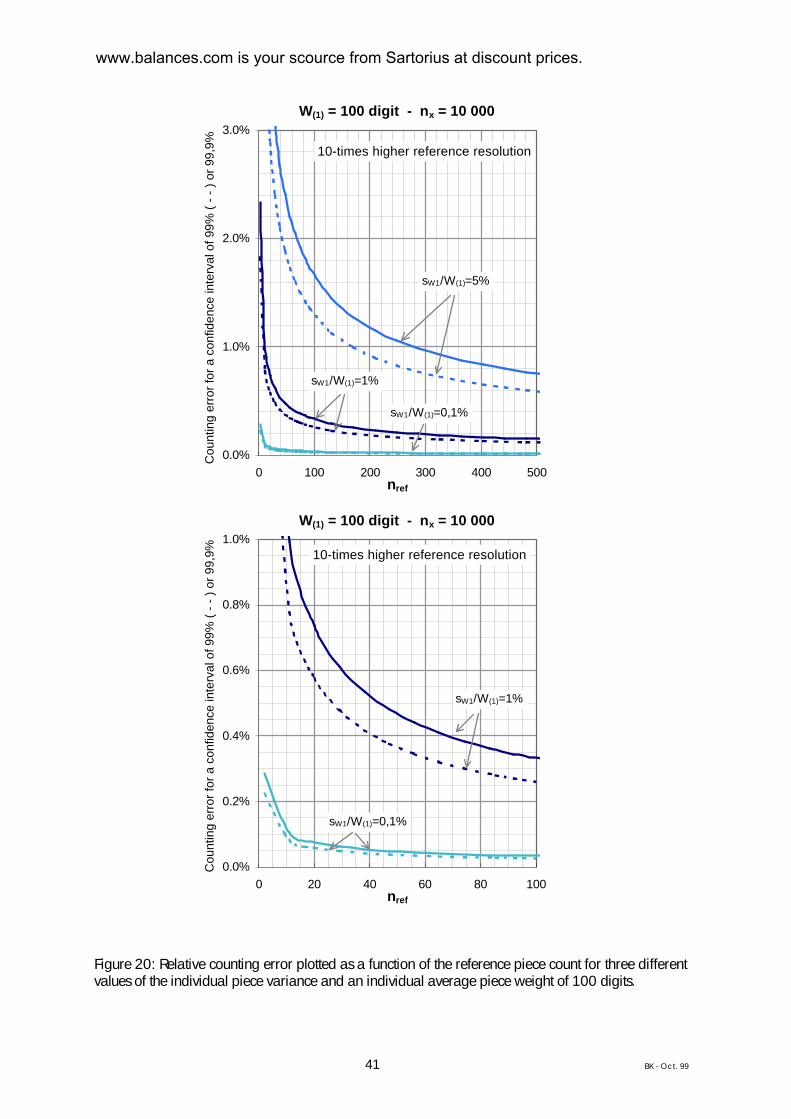
For the graphs (Figures 11, 14, 17, and 20), a scale with an internal resolution 10 times higherthan the display resolution was used to determine the reference weight, i.e., sWref

is calculated with

0.1 digit. The standard deviation of the total weight sWx continues to be calculated with 1 digit.

The same holds true for the next graphs (12 and 18): here, a scale with an internal resolution 100times higher than the display resolution was used to determine the reference weight 4. In otherwords, sWref

is calculated with 0.01 digit to determine the counting accuracy, and sWx is calcula-

ted with 1 digit.

The graphs provide a good orientation guide for many counting applications. To enable the coun-ting accuracy to be calculated for each individual case, the EXCEL file “ACCURACY” is includedwith this handbook. After 10 individual average piece weights, the readability of the scale, andthe target piece count and reference piece count are entered in the spreadsheet, the relative coun-ting error is calculated with a confidence interval of 95%, 99% and 99.9%. In addition, the ma-ximum deviation from the target piece count is indicated, and a determination is made as to whe-ther or not counting that is accurate down to the last component is possible under the selectedconditions. Examples of printouts are included in the appendix (p. 43).

If the absolute error when counting may not be larger than 1 piece, the condition

∆x = t s 0,5 x⋅ <

must be fulfilled.

4 The same is true if a separate reference scale with a readability of 1/100 of the bulk weigher is used.


16 BK - Oct. 99

Reference Sample Updating for Optimization

As explained in the previous chapter on calculating the counting error, one can generally improvethe counting accuracy with larger reference piece counts.

Because it is very tedious to count a large number of mostly small, individual parts by hand, and,above all, because a (systematic) counting error, which would distort the entire counting result, caneasily result, all Sartorius scales equipped with counting application software feature a referencesample updating option.

Starting out with a small reference piece count, this feature gradually increases it until the desiredreference piece count has been reached. Certain conditions must be observed in the process toensure that the counting error when determining the reference piece count is always less than 1piece ( < ± 0.5).

n 2 n 2 n1ref 2ref 1ref+ ≤ ≤ ⋅ ( 11)

For example, in the first step, the reference weight W1ref is determined based on n1ref = 10 hand-counted, individual parts. After adding 2 to 20 additional, individual parts, the piece count n2ref iscalculated based on the weight W2ref according to the relationship (3) on page 4:

n WnW2ref 2ref

1ref

1ref

= ⋅ . ( 12)

Software for Sartorius scales allows reference sample updating for optimization• if the current piece count is less than double the original piece count (n2ref ≤ 2 ⋅ n1ref),• if the deviation from the next whole number of n2ref is < ± 0.3,• and as long as the piece count nref is < 100.

If these conditions are met, the value nW

1ref

1ref

for calculating the target piece count or for the next

step in reference optimization is substituted by nW

2ref

2ref

. The resulting equation is:

n WnW

or n WnW

3ref 3ref2ref

2refx x

2ref

2ref

= ⋅ = ⋅ . ( 13)

The following example, with the help of the accompanying graph, will illustrate and provide abetter understanding of reference optimization. With the exception of the piece count nx, thegraph corresponds to Figure 16 on page 37. (Figures 15 through 20 can be used accordingly).• the counting error should not exceed 0.5 %,

• fluctuations in the weights of the parts being counted amount to sW

W1

(1)

= 1 % when the stan-

dard deviation of sW1 = 0.012 g• one digit on the scale corresponds to 0.1 g• the average individual piece weight is W(1) = 1.2 g, corresponding to ∼ 10 digits

Since the predefined counting error tolerance may not exceed 0.5 %, a reference piece count of atleast 80 results from the curve (with a confidence interval of 99.9 %).


17 BK - Oct. 99

In the first step of reference sample updating, a reference piece count of 10 is selected. The coun-ting error for this piece count is ∼ 3 %, i.e., 0.3 part for every 10 parts. This ensures accuratecounting down to the last component, and the number of reference samples can, therefore, be rai-sed by 10.

For a reference piece count of 20, the counting error is ∼ 1.5 %, under the given conditions, i.e.,0.3 part for every 20 parts. Accurate counting down to the last component is again ensured.

If the piece count is raised to 40 in the next step, the counting error is still ∼ 0.9 %, i.e., a maxi-mum of 0.36 part for every 40 parts. The counting error remains less than 1 piece or < ± 0.5,and the next time the piece count is doubled, a reference piece count of 80 will already be re-ached. At this point, the actual counting task can begin with the desired degree of counting accu-racy.

Figure 4: Illustration of reference sample updating

W(1) = 10 digits - nx = 1 000

0.0%

0.5%

1.0%

1.5%

2.0%

2.5%

3.0%

3.5%

0 10 20 30 40 50 60 70 80 90 100nref

Cou

ntin

g er

ror

for

a co

nfid

ence

inte

rval

of 9

9 %

( -

- )

or

99.9

%

sW1/W(1)=1,0%


18 BK - Oct. 99

Selecting the “Right” Counting Scale

When selecting a counting scale, the general rules apply. Above all, the following should be ta-ken into consideration:• the expected maximum load or the total weight which will be placed on the scale

(If necessary, the total weight can be divided into smaller amounts, which can then be addedtogether in the totalizing memory of the scale.)

• the readability, which is determined by the desired accuracy of the counting result. This, inturn, depends on− the absolute quantity of the reference weight,− the accuracy with which the (average) individual piece weight can be read on the display, and− the accuracy with which the reference weight can be read on the display

In general, the following applies: For determining the reference, a higher internal resolution of theweighing range – or the use of a reference scale with a higher resolution than that of the bulkweigher – greatly improves the counting accuracy and, in addition, reduces the required referencepiece count.

The four tables that follow should simplify the selection of a suitable scale. All values are calculatedfor a confidence interval of 99.9 %.

Determining the Suitable Readability of a Scale

First of all, a decision must be made about the degree of accuracy with which the parts are to becounted – this determines which table (counting error < 1 %, < 0.5 %, < 0.1 % or < 0.05 %) isapplicable.

The next parameter that must be known is the relative standard deviation (s/W(1)) of the parts tobe counted – the tables include examples for four different values (5 %, 1 %, 0.5 % and 0.1).

The individual average piece weights are indicated in digits, i.e., an immediate reference is ma-de regarding the readability of the scale. Refer to the lines in the table marked with ¡ (10-timeshigher internal resolution) or ¡¡ (100-times higher internal resolution) when using a reference sca-le or a scale with a higher internal resolution to determine the reference.

A readability of 100 digits related to the average individual piece weight with 100-times higherinternal resolution rather than only 10-times higher resolution no longer presents an appreciableadvantage for determining the reference.

The last column in the tables shows the reference piece count at which the corresponding countingerrors are reached or fall short of being reached. If the calculated reference piece count is > 500,the counting error entered will be considered “impossible” to attain. The smallest entry for the refe-rence piece count is 10, even if the error is clearly smaller than 1 % and reference piece countssmaller than 10 are being calculated (e.g., at the bottom of Table 1, where the standard deviationof the individual parts is 0.1 %).


19 BK - Oct. 99

Example:

The desired counting error is ≤ 0.5 % – therefore, Table 3 should be selected.

The average weight of the individual parts is 1.3 g. This weight was calculated based on theweights of 10 parts as described in the section entitled “Fundamentals of Statistics” on page 5.(For information on sampling, see also chapter „Removal of Reference Samples“, page 24.)

The standard deviation of the individual average piece weight is 0.0125 g. Therefore, the relati-

ve standard deviation is: s

W0,0125g

1,3g0,0096 0,96% 1%

(1)

= = = ≈

Thus in Table 3, the second section from the top is applicable: with a scale readability of 1 g(individual average piece weight =1.3 g ≈ 1 digit), a counting error < 0.5 % could not be at-tained with the parts in the example. For readabilities of 0.1 g or 0.01 g (individual averagepiece weight =1.3 g ≈ 10 digits or ≈ 100 digits), the desired counting error is attainable undervarious conditions listed below – with the reference piece counts indicated in column three:• When the readability of the scale is 1 g, and the resolution is 10-times (or 100-times) higher,

with at least 92 (or 45) reference samples the required counting error can be attained.• A reference sample piece count of at least 92 is required when the readability of the scale is

0.1 g and the reference resolution = total weight resolution. A reference sample piece count ofat least 45 is necessary for a scale with a 10-times higher internal resolution. However, a refe-rence sample piece count of 44 is sufficient for a 100-times higher resolution to reduce the se-lected counting error to below 0.5 %.

• When the readability of the scale is 0.01 g, and the reference sample resolution = actualpiece count resolution or 10-times to 100-times higher resolution, reference piece counts of atleast 44 or 45 can be used to attain the counting error of 0.5 %. With the parts in the examplescales with higher resolution no longer present an advantage for determining a “better“ countingresult.

In all cases, nref is so high that the automatic reference optimization function should be used.With this feature, the required reference piece count is achieved quickly – in three or four steps. Italso largely rules out a systematic counting error that could occur while counting the referencesamples by hand. Such an error would render the entire counting result unusable.


20 BK - Oct. 99

Table 2: Selection of a suitable scale when the maximum accepted counting error is 1 % for various re-lative standard deviations of the individual parts.(10,000 parts were used as a basis for calculation; i.e., for low piece counts such as 100 parts,the error can be up to ∼ 0.5 % larger than indicated above. See also Figures 7 and 8.)

A counting error of ± 1 % corresponds to counting that is accurate down to the last componentwhen the total number of parts counted is 50. When 1,000 parts are counted, the result can de-viate from the target by up to ± 10 parts.

Counting error < 1 % at a confidence interval of 99,9%

Relative Minimumstandard deviation Individual weight reference

of the parts to be counted W(1) piece counts/W(1) in digits nref

1 5001 ¡ 2851 ¡¡ 280

10 2835% 10 ¡ 280

10 ¡¡ 280100 280100 ¡ 280100 ¡¡ 280

1 3361 ¡ 391 ¡¡ 12

10 401% 10 ¡ 12

10 ¡¡ 11100 12100 ¡ 11100 ¡¡ 11

1 3321 ¡ 351 ¡¡ 10

10 350.5% 10 ¡ 10

10 ¡¡ 10100 10100 ¡ 10100 ¡¡ 10

1 3301 ¡ 331 ¡¡ 10

10 330.1% 10 ¡ 10

10 ¡¡ 10100 10100 ¡ 10100 ¡¡ 10

¡: 10-times higher internal resolution

¡¡: 100-times higher internal resolution


21 BK - Oct. 99

Counting error < 0,5 % at a confidence interval of 99,9%


of the parts to be counted W(1) piece counts/W(1) in digits nref

independent5% of the scale not possible

selected

1 not possible1 ¡ 921 ¡¡ 45

10 921% 10 ¡ 45

10 ¡¡ 44100 45100 ¡ 44100 ¡¡ 44


10 720.5% 10 ¡ 14

10 ¡¡ 11100 14100 ¡ 11100 ¡¡ 11


10 670.1% 10 ¡ 10

10 ¡¡ 10100 10100 ¡ 10100 ¡¡ 10



Table 3: Selection of a suitable scale when the maximum accepted counting error is 0,5 % for variousrelative standard deviations of the individual parts.(10,000 parts were used as a basis for calculation; i.e., for low piece counts such as 100 parts,the error can be up to ∼ 0.5 % larger than indicated above. See also Figures 7 and 8.)

A counting error of ± 0.5 % corresponds to counting that is accurate down to the last componentwhen the total number of parts counted is 100. When 1,000 parts are counted, the result candeviate from the target by up to ± 5 parts.


22 BK - Oct. 99

Table 4: Selection of a suitable scale when the maximum accepted counting error is 0.1 % for variousrelative standard deviations of the individual parts.(10,000 parts were used as a basis for calculation; i.e., for low piece counts such as 100 parts,the error can be up to ∼ 0.5 % larger than indicated above. See also Figures 7 and 8.)

A counting error of ± 0.1 % corresponds to counting that is accurate down to the last componentwhen the total number of parts counted is 500. When 1,000 parts are counted, the result candeviate from the target by up to ± 1 part.



of the parts to be counted W(1) piece count

s/W(1) in digits nref


selected


selected

1 not possible1 ¡ not possible1 ¡¡ 320

10 not possible10 ¡ 283

0.5% 10 ¡¡ 279100 283100 ¡ 279100 ¡¡ 279

1 not possible1 ¡ 3551 ¡¡ 42

10 33610 ¡ 39

0.1% 10 ¡¡ 12100 39100 ¡ 12100 ¡¡ 11




23 BK - Oct. 99

Table 5: Selection of a suitable scale when the maximum accepted counting error is 0.05 % for va-rious relative standard deviations of the individual parts.(10,000 parts were used as a basis for calculation; i.e., for low piece counts such as 100 parts,the error can be up to ∼ 0.5 % larger than indicated above. See also Figures 7 and 8.)

A counting error of ± 0,05 % corresponds to counting that is accurate down to the last componentwhen the total number of parts counted is 1,000.



of the parts to be counted W(1) piece count

s/W(1) in digits nref


selected


selected

independent0.5% of the scale not possible

selected

1 not possible1 ¡ not possible

0.1% 1 ¡¡ 13510 not possible10 ¡ 9210 ¡¡ 45

100 92100 ¡ 45100 ¡¡ 44




24 BK - Oct. 99

Removal of Reference Samples

When counting by weighing, a factor is calculated based on the number of reference samples andthe reference weight. With the help of this factor, the piece count can be inferred from the totalweight (see equation 3).

The reference samples represent only a small fraction of the total number of parts to be counted. Itis basically assumed that the qualities of this small number of parts correspond to those of the totalnumber of parts (that they paint a “representative picture of the population”). Only then can stati-stical formulas that are based on a Gaussian distribution curve be used. A corresponding standardoperating procedure for sampling is of crucial significance for the usability of the counting result.

Random or statistical errors that can occur when determining the piece count are covered extensive-ly in chapter “Calculating the Counting Error ” page 11. The sampling error as a systematic error,however, can easily become much larger than the statistical error. This means that the referencesamples must be carefully selected and counted by hand accordingly.

Theoretically, each individual part from the total quantity must have the same probability of beingincluded in the reference sample.

In practice this means that, for example, several individual parts are removed from a large contai-ner at 10 different locations (e.g., from the top, the bottom, the front, ...). These parts are then mi-xed together well. Next, this group of parts is divided in half, in fourths, and then in eighths. Final-ly, one part for the reference sample is taken in succession from each of these small groups. Alter-natively, one can take small samples at regular intervals while the small parts are being manufactu-red, mix these samples together, divide them into groups, and finally remove parts from each smallgroup for the determination of the reference weight.

Difficulties can arise if, for example, small parts are being produced by two machines and the partsmanufactured by machine 1 have a slightly different mean value than those produced by machine2. These conditions are demonstrated in Figures 5 and 6.

In this case, one can either• count parts only from machine 1 or machine 2, which assumes a smaller individual piece varia-

tion and, accordingly, a greater accuracy of the counting result,• or mix the parts from machine 1 and machine 2 at a defined proportion for sampling both whi-

le determining the reference weight and while counting. However, one must expect a largerindividual piece variation and, accordingly, a larger counting error.

The graph shows (see Figure 5) that the total distribution becomes increasingly broader as the di-stance between the mean values of the individual distributions increases. In the process, the stan-dard deviation or the variance also continues to increase. How one actually works under suchconditions depends mainly on the acceptable counting error. If the mean values of the individualdistributions are too far apart, the cumulative distribution (see Figure 6) no longer results in aGaussian distribution curve, and the basis for using the statistical calculations applied here no lon-ger exists. This means that under such conditions, parts manufactured by different machines maynot be counted together.


25 BK - Oct. 99

n

x ( +2)1

x1 x2

Figure 5: Frequency distribution of the parts manufactured by machine 1 with the mean value x1 and

those produced by machine 2 with the mean value x2 ; frequency distribution for the combination of

parts from machines 1 and 2 with the mean value x (1 2)+

n

x1 x2

Figure 6: Frequency distribution of the parts manufactured by machine 1 with the mean value x1 and

those produced by machine 2 with the mean value x2 ; a “bell curve” no longer results when the parts

from machines 1 and 2 are added together, i.e., the parts no longer meet the fundamental requirementfor the applicability of the statistical calculations.


26 BK - Oct. 99

Appendix


27 BK - Oct. 99

t Factor or Student Factor for Calculating the Ranges of Dispersion (Scatter)

To calculate the scatter ∆x t s= ⋅ with a particular confidence interval, the t factors are required.

t factor

Confidence interval 95 % 99 % 99,9 %n = 6 2,57 4,03 6,86n = 10 2,26 3,25 4,781n = 20 2,09 2,86 3,883n = 50 2,009 2,678 3,469n= 100 1,984 2,626 3,390n = ∞ 1,960 2,576 3,291


28 BK - Oct. 99

Graphs Determining the Counting Accuracy

Comments on the following graphs see page 14.

W(1) = 10 digits, 10-times higher reference resolution nx = 100 to nx = 10000

0.00%

1.00%

2.00%

3.00%

4.00%

5.00%

0.0% 1.0% 2.0% 3.0% 4.0% 5.0%sW(1)/W(1)

100

500

1000

10000

100

500

1000

10000

Cou

ntin

g er

ror

for

a co

nfid

ence

inte

rval

of 9

9.9

%

nref=100

nref=10

Figure 7: Relative counting error plotted as a function of the relative standard deviation of the individu-al parts for various target piece counts nx.

The graph shows that the smaller the total number of parts to be counted is, the larger the relativecounting error becomes. For example, for a relative standard deviation of 3.0% and a referencepiece count of 10, the counting error equals• 3.1 % for 10,000 parts• 3.2 % for 1,000 parts• and 3.3 % for 100 parts.

For a relative standard deviation of 3 % and a reference piece count of 100, the counting errorcorresponds to• 1.0 % for 10,000 parts• 1.1 % for 1,000 parts• and 1.4 % for 100 parts.


29 BK - Oct. 99

W(1) = 10 digits, 10-times higher reference resolution nx = 100 to nx = 10000

0.00%

1.00%

2.00%

3.00%

4.00%

5.00%

0 10 20 30 40 50 60 70 80 90 100nref

100

1000

10000

100

1000

10000

100

1000

10000

sW1/W(1) = 1,0 %sW1/W(1) = 0,1 %

sW1/W(1) = 5,0 %

Cou

ntin

g er

ror

for

a co

nfid

ence

inte

rval

of 9

9,9%

Figure 8: Relative counting error plotted as a function of the reference piece count for various targetpiece counts nx

The graph shows that the smaller the total number of parts to be counted is, the larger the relativecounting error becomes. For example, for a reference piece count of 80 and a relative standarddeviation of 1.0%, the counting error equals• 0.37 % for 10,000 parts (corresponds to ± 37 parts)• 0.38 % for 1,000 parts (corresponds to ± 4 parts)• and 0.59 % for 100 parts (corresponds to ± 1 part).

For a reference piece count of 80 and a relative standard deviation of 0.1 %, the counting error isequal to• 0.10 % for 10,000 parts (corresponds to ± 10 parts)• 0.10 % for 1,000 parts (corresponds to ± 1 part)• and 0.34 % for 100 parts, which corresponds to ± 0.3 part and means that counting that is accurate

down to the last component is possible under these conditions.


30 BK - Oct. 99

W(1) = 1 digit - nx = 10 000

0.0%

2.0%

4.0%

6.0%

8.0%

10.0%

0% 1% 2% 3% 4% 5% 6% 7% 8%sW(1)/W(1)

Cou

ntin

g er

ror

for

a co

nfid

ence

inte

rval

of 9

9% (

- -

) o

r 99

,9%

nref=50

nref=500

nref=100

Figure 9: Relative counting error plotted as a function of the individual piece variance for various refe-rence piece counts and an individual average piece weight of 1 digitreference resolution = total piece count resolution.

When the relative standard deviation of the individual parts s

WW

(1)

(1) is known in %, the attainable

counting error can be read off the y axis for reference piece counts of 50, 100 or 500.


31 BK - Oct. 99

W(1) = 10 digits - nx = 10 000

0.0%

2.0%

4.0%

6.0%

8.0%

10.0%

0% 1% 2% 3% 4% 5% 6% 7% 8%sW(1)/W(1)

nref=50

nref=500

nref=100

nref=10

Cou

ntin

g er

ror

for

a co

nfid

ence

inte

rval

of 9

9% (

- -

) o

r 99

,9%

Figure 10: Relative counting error plotted as a function of the individual piece variance for various re-ference piece counts and an individual average piece weight of 10 digitsreference resolution = total piece count resolution.


WW

(1)


counting error can be read off the y axis for reference piece counts of 10, 50, 100 or 500.


32 BK - Oct. 99

W(1) = 10 digits - nx = 10 000

0.0%

2.0%

4.0%

6.0%

8.0%

10.0%

0% 1% 2% 3% 4% 5% 6% 7% 8%sW(1)/W(1)

nref=50

nref=500

nref=100

nref=10

10-times higher reference resolution

Cou

ntin

g er

ror

for

a co

nfid

ence

inte

rval

of 9

9% (

- -

) o

r 99

,9%

Figure 11: Relative counting error plotted as a function of the individual piece variance for various re-ference piece counts and an individual average piece weight of 10 digitsreference resolution = 10 ⋅⋅ total piece count resolution.


WW

(1)



The advantage of higher reference resolution is especially noticeable when the values of the indivi-dual piece variance are low. When the individual piece variance is great, the counting accuracyis limited by this “disproportion of the parts.”


33 BK - Oct. 99

W(1) = 10 digits - nx = 10 000

0.0%

2.0%

4.0%

6.0%

8.0%

10.0%

0% 1% 2% 3% 4% 5% 6% 7% 8%sW(1)/W(1)

nref=50

nref=500

nref=100

nref=10

Cou

ntin

g er

ror

for

a co

nfid

ence

inte

rval

of 9

9% (

- -

) o

r 99

,9%

100-times higher reference solution



WW

(1)



The advantage of higher reference resolution is especially noticeable when the values of the indivi-dual piece variance are low (see the previous graph). When the individual piece variance isgreat, the counting accuracy is limited by the weight variance of the individual parts.


34 BK - Oct. 99

W(1) = 100 digits - nx = 10 000

0.0%

2.0%

4.0%

6.0%

8.0%

10.0%

0% 1% 2% 3% 4% 5% 6% 7% 8%sW(1)/W(1)

nref=50

nref=500

nref=100

nref=10

Cou

ntin

g er

ror

for

a co

nfid

ence

inte

rval

of 9

9% (

- -

) o

r 99

,9%

Figure 13: Relative counting error plotted as a function of the individual piece variance for various re-ference piece counts and an individual average piece weight of 100 digitsreference resolution = total piece count resolution.


WW

(1)


counting error can be read off the y axis for reference piece counts of 10, 50, 100 or 500. Theresults are equal to those that also would be obtained using a scale with a readability correspon-ding to 10 digits of the individual average piece weight at 10 times higher reference resolution.


35 BK - Oct. 99

W(1) = 100 digits - nx = 10 000

0.0%

2.0%

4.0%

6.0%

8.0%

10.0%

0% 1% 2% 3% 4% 5% 6% 7% 8%sW(1)/W(1)

nref=50

nref=500

nref=100

nref=10

Cou

ntin

g er

ror

for

a co

nfid

ence

inte

rval

of 9

9% (

- -

) o

r 99

,9%




WW

(1)



The advantage of higher reference resolution is especially noticeable when the values of the indivi-dual piece variance are low (see the previous graph). When the individual piece variance isgreat, the counting accuracy is limited by the variance of the average weight of the individualparts.


36 BK - Oct. 99

Figure 15: Relative counting error plotted as a function of the reference piece count for three differentvalues of the individual piece variance and an individual average piece weight of 1 digit.

W(1) = 1 digit – nx = 10 000

0.0%

1.0%

2.0%

3.0%

0 100 200 300 400 500nref

sW1/W(1)=1%

sW1/W(1)=0,1%

sW1/W(1)=5%

Cou

ntin

g er

ror

for

a co

nfid

ence

inte

rval

of 9

9% (

- -

) o

r 99

,9%

W(1) = 1 digit – nx = 10 000

0.0%

2.0%

4.0%

6.0%

8.0%

10.0%

0 20 40 60 80 100nref

sW1/W(1)=5%

sW1/W(1)=1%

sW1/W(1)=0,1%

Cou

ntin

g er

ror

for

a co

nfid

ence

inte

rval

of 9

9% (

- -

) o

r 99

,9%

sW1/W(1)=1%

sW1/W(1)=0,1%

sW1/W(1)=5%


37 BK - Oct. 99

Figure 16: Relative counting error plotted as a function of the reference piece count for three differentvalues of the individual piece variance and an individual average piece weight of 10 digits.

W(1) = 10 digits - nx = 10 000

0.0%

1.0%

2.0%

3.0%

0 100 200 300 400 500nref

sW1/W(1)=5%

sW1/W(1)=1%

sW1/W(1)=0,1%

Cou

ntin

g er

ror

for

a co

nfid

ence

inte

rval

of 9

9% (

- -

) o

r 99

,9%

W(1) = 10 digits - nx = 10 000

0.0%

1.0%

2.0%

3.0%

4.0%

5.0%

0 20 40 60 80 100nref

sW1/W(1)=5%

sW1/W(1)=1%

sW1/W(1)=0,1%

Cou

ntin

g er

ror

for

a co

nfid

ence

inte

rval

of 9

9% (

- -

) o

r 99

,9%


38 BK - Oct. 99


W(1) = 10 digits - nx = 10 000

0.0%

1.0%

2.0%

3.0%

0 100 200 300 400 500nref

sW1/W(1)=5%

sW1/W(1)=1%

sW1/W(1)=0,1%

Cou

ntin

g er

ror

for

a co

nfid

ence

inte

rval

of 9

9% (

- -

) o

r 99

,9%


W(1) = 10 digits - nx = 10 000

0.0%

0.5%

1.0%

1.5%

2.0%

0 20 40 60 80 100nref

sW1/W(1)=5%

sW1/W(1)=1%

sW1/W(1)=0,1%

Cou

ntin

g er

ror

for

a co

nfid

ence

inte

rval

of 9

9% (

- -

) o

r 99

,9%



39 BK - Oct. 99


W(1) = 10 digits - nx = 10 000

0.0%

1.0%

2.0%

3.0%

0 100 200 300 400 500nref

sW1/W(1)=5%

sW1/W(1)=1%

sW1/W(1)=0,1%

Cou

ntin

g er

ror

for

a co

nfid

ence

inte

rval

of 9

9% (

- -

) o

r 99

,9%


W(1) = 10 digits - nx = 10 000

0.0%

0.2%

0.4%

0.6%

0.8%

1.0%

0 20 40 60 80 100nref

sW1/W(1)=1%

sW1/W(1)=0,1%


Cou

ntin

g er

ror

for

a co

nfid

ence

inte

rval

of 9

9% (

- -

) o

r 99

,9%


40 BK - Oct. 99


W(1) = 100 digits – nx = 10 000

0.0%

1.0%

2.0%

3.0%

0 100 200 300 400 500nref

sW1/W(1)=5%

sW1/W(1)=1%

sW1/W(1)=0,1%

Cou

ntin

g er

ror

for

a co

nfid

ence

inte

rval

of 9

9% (

- -

) o

r 99

,9%

W(1) = 100 digits - nx = 10 000

0.0%

0.5%

1.0%

1.5%

0 20 40 60 80 100nref

sW1/W(1)=1%

sW1/W(1)=0,1%

sW1/W(1)=5%

Cou

ntin

g er

ror

for

a co

nfid

ence

inte

rval

of 9

9% (

- -

) o

r 99

,9%


41 BK - Oct. 99


W(1) = 100 digit - nx = 10 000

0.0%

1.0%

2.0%

3.0%

0 100 200 300 400 500nref

sW1/W(1)=5%

sW1/W(1)=1%

sW1/W(1)=0,1%


Cou

ntin

g er

ror

for

a co

nfid

ence

inte

rval

of 9

9% (

- -

) o

r 99

,9%

W(1) = 100 digit - nx = 10 000

0.0%

0.2%

0.4%

0.6%

0.8%

1.0%

0 20 40 60 80 100nref

sW1/W(1)=1%

sW1/W(1)=0,1%


Cou

ntin

g er

ror

for

a co

nfid

ence

inte

rval

of 9

9% (

- -

) o

r 99

,9%


42 BK - Oct. 99

Calculating the Counting Accuracy – Examples of Printouts from the EXCEL File

With the help of the EXCEL file entitled “ACCURACY.XLS,” the counting error can easily be calculatedfor every counting task. The individual weights of at least 6, preferably 10, carefully selected, re-presentative individual parts are determined and entered in the fields highlighted in green.

The mean value and the standard deviation are calculated and shown in the yellow fields as essen-tial results. (Additionally, the minimum and maximum weights and the standard deviation areshown in the gray fields.)

Entries must be made in the remaining green fields. The following information is required:• the (approximate) number of individual parts to be counted,• the reference piece count,• the readability of the scale• the readability of the scale used to determine the reference or the reference scale.

The formulas discussed in the first two chapters are used for calculation.

The standard deviation of the counting result is then indicated as an absolute value and as a per-centage in the result field.

In addition, the maximum deviation from the target piece count and the relative counting error areindicated for the statistical probabilities of 95 %, 99 % and 99.9 %.

Examples of printouts for various counting conditions appear on the following pages.


43 BK - Oct. 99


The counting accuracy is mainly influenced by the variance of the weight of the individual parts.

Therefore, the weights of 10 different individual parts must first be determined.

The smallest piece weight should amount to at least 10 digits of the scale display - 100 digitswhen a higher degree of accuracy is required.

Part Indiv. Weight g Statistical Evaluation

1 2.0020 g Largest individual value 2.0020 g2 2.0000 g3 2.0000 g Smallest individual value 1.9980 g4 2.0010 g5 2.0000 g Maximum deviation 0.0040 g6 2.0000 g (largest value minus smallest value)

7 1.9980 g Avg. weight of individual parts 2.0001 g8 1.9990 g9 2.0000 g Standard deviation 0.0011 g

10 2.0010 g Relative standard deviation 0.06 %

Information Necessary for Calculating the Counting Accuracy

Number of parts to be counted (target piece count) 1002

Reference piece count 10

1 digit of the scale used 0.1 g

1 digit of the (reference) scale used or of the internal resolution 0.01 g

Total weight 2004 g

Result of the Counting Accuracy

Standard deviation of the piece count 0.533

Relative standard deviation 0.05 %

Statistical Probability

95% 99% 99.9%

Maximum deviation from target piece count ± 1 1 2Relative counting error ± 0.10% 0.14% 0.18%Counting accurate to last component possible no no noFulfills the condition of the FPVO yes yes yes


44 BK - Oct. 99


The counting accuracy is mainly influenced by the variance of the weight of the individual parts.

Therefore, the weights of 10 different individual parts must first be determined.

The smallest piece weight should amount to at least 10 digits of the scale display - 100 digitswhen a higher degree of accuracy is required.

Part Indiv. Weight mg Statistical Evaluation

1 23.1000 mg Largest individual value 23.3000 mg2 23.2000 mg3 23.3000 mg Smallest individual value 23.0000 mg4 23.2000 mg5 23.1000 mg Maximum deviation 0.3000 mg6 23.2000 mg (largest value minus smallest value)

7 23.1000 mg Avg. weight of individual parts 23.1600 mg8 23.2000 mg9 23.0000 mg Standard deviation 0.0843 mg

10 23.2000 mg Relative standard deviation 0.36 %

Information Necessary for Calculating the Counting Accuracy

Number of parts to be counted (target piece count) 300

Reference piece count 10

1 digit of the scale used 0.1 mg

1 digit of the (reference) scale used or of the internal resolution 0.01 mg

Total weight 6948 mg

Result of the Counting Accuracy

Standard deviation of the piece count 0.351

Relative standard deviation 0.12 %

Statistical Probability

95% 99% 99.9%

Maximum deviation from target piece count ± 1 1 1Relative counting error ± 0.23% 0.30% 0.39%Counting accurate to last component possible no no noFulfills the condition of the FPVO yes yes yes


45 BK - Oct. 99

Questions about Counting

1. On which fundamental equation is “counting by weighing” based?

2. Which quantities influence the counting accuracy, and which quantity has the greatest influ-

ence?

3. How does the reference piece count influence the accuracy of the counting result?

4. What is the advantage of reference optimization? Within what range should the increase in

the piece count lie?

5. What is meant by “representative sampling,” and why is sampling while selecting the refe-

rence samples of such great significance?

6. Can you determine the standard deviation for the following series of individual weights?

11.10 g / 10.98 g / 10.96 g / 10.99 g / 11.02 g / 11.06 g / 11.02 g / 11.00 g / 11.03 g /

10.92 g

7. If you calculated the standard deviation “by hand,” you already know the mean value of the

weights above. In case you simply used the applicable EXCEL function, please use the

function at this time to calculate the mean value. How great is the relative standard devia-

tion?

8. Which scale would you recommend to someone who would like to count the parts in the

example in question 6 accurately down to the last component in groups of 800?


Answers to the Questions

1. n WnWx x

ref

ref

= ⋅

2. The variance of the average individual piece weight has the greatest influence on the coun-

ting accuracy.

Other influence quantities: reference piece count, total piece count, variance of the refe-

rence weight, variance of the total weight

3. In general, the larger the reference piece count is, the greater becomes the degree of coun-

ting accuracy.

4. For large reference piece counts, it is not necessary to count all individual parts by hand,

rather only the first 10 or 15 parts, for example. This reduces the probability of a counting

error occurring during determination of the reference piece count.

During reference optimization, the reference piece count should be increased by at least 2

parts. A maximum of twice the original reference piece count may be used.

5. For a description of sampling, see p. 24.

Based on the properties (here the weight) of a few parts, an inference is drawn regarding

the properties of a large number of parts – with the help of statistical methods. If the refe-

rence samples do not represent the population of all parts, the basic requirement for the

applicability of the statistical calculations is missing.

6. The value is calculated according to the general formula (equation 6, Fundamentals of Sta-

tistics)

( )s 1n 1

x xii 1

n 2

=−

⋅ −=∑ = ± 0,051g

In EXCEL, this corresponds to the STDEV(...) function, not the STDEVP(…) function.

7. The mean value x is 11.01 g. (corresponds to the EXCEL function AVERAGE(…).)

The relative standard deviation is sx

0,0046 0,46%= = .

8. Table 5 on p. 23 shows that it is impossible to count 1,000 parts accurately down to the last

component when the relative standard deviation of the individual parts is 0.5 %. Table 4

on p. 22, shows that an error of ± 0.1 % or ± 1 related to 1,000 parts is attainable (e.g.,

with a scale readability of 1 g and 100-times higher internal resolution or a scale readabili-

ty of 0.1 g and 10-times higher internal resolution and a reference piece count of 279 (use

the reference optimization function).

If you use the Excel file entitled “ACCURACY.XLS,” you will see that under the given conditions,

it is possible to count the parts accurately down to the last component with a reference

piece count of 290 and a confidence interval of 95 %. Counting with a confidence interval


47 BK - Oct. 99

of 99 % or even 99.9 %, however, is not possible. This means that the quantity weighed is

really 800 parts in 95 out of 100 counting operations. In 5 out of 100 cases, the actual

piece count on the scale can be 801 or 799 when the display shows 800.


48 BK - Oct. 99

Register

AAccuracy • 5, 11Approximation Of The Standard Deviation • 7Average Weight • 4

CConfidence Interval • 9Counting Accuracy • 13, 14Counting Accurate Down To The Last Component

• 15Counting Error • 11, 16, 24Counting Scale • 2, 3, 18Cumulative Distribution • 24

DDistribution Curve • 8

EError • 5

GGaussian Distribution Curve • 9, 24

MMaximum Load • 18Mean Value • 5, 6

PPiece Count • 4, 24Population • 24

Probability • 24

RRandom Errors • 5Readability • 18Reference Piece Count • 4, 16, 24Reference Sample Quantity • 4, 11, 16Reference Sample Updating For Optimization •

16Reference Weight • 16, 24Relative Standard Deviation • 7Resolution • 18

SSampling • 24Sampling Error • 24Scatter Of The Individual Values • 10Standard Deviation • 6, 9, 24Statistical Error • 5, 24Statistical Probability • 9Systematic Error • 5, 24

TTotal Weight • 24True Value • 6

VVariance • 7, 24

WWeight • 4


manual of weighing applications - analytical … · manual of weighing applications part 2 ... the...

Documents