manual / user guide / handbook - reentry.esoc.esa.int · handbook esa re-entry ... after...

ESA UNCLASSIFIED - For Official Use

Prepared by Space Debris Office

Reference GEN-REN-MAN-00232-OPS-GR

Issue/Revision 0.0

Date of Issue 3/5/2018

Status Issued

esoc European Space Operations Centre

Robert-Bosch-Strasse 5 D-64293 Darmstadt

Germany T +49 (0)6151 900

F +49 (0)6151 90495 www.esa.int

MANUAL / USER GUIDE / HANDBOOK

ESA Re-entry Prediction Front-end User Guide


/17


Issue Date 3/5/2018 Ref GEN-REN-MAN-00232-OPS-GR

Table of contents:

1 INTRODUCTION ...................................................................................... 3 2 CONTENT PAGES ..................................................................................... 3 2.1 General page ..................................................................................................................... 3 2.2 Re-entry Predictions page ................................................................................................ 4 2.3 Detail page ........................................................................................................................ 6 3 RESTRICTED ACCESS PAGES .................................................................. 6 4 BASICS OF PREDICTING RE-ENTRY EVENTS .......................................... 6 5 REFERENCES ......................................................................................... 17


/17



1 INTRODUCTION

This document provides a general introduction to the European Space Agency’s Re-entry Predictions Front-end hosted at https://reentry.esoc.esa.int . The front-end services as an interface for the general public as well as expert users to obtain predictions on where and when artificial space objects will re-enter the Earth atmosphere. As a rule of thumb, the re-entry prediction data is updated daily. The front-end is separated in two parts: A general area covering background information on re-entries and the user login functionality, and an area dedicated to upcoming re-entry predictions. Furthermore, this document will cover the specifics in individual re-entry events. The hosted content is subject to the physics involved with re-entry predictions and can contain errors. We welcome feedback and it can be provided to an admin via the Ask Admin functionality or via e-mail to [email protected].

2 CONTENT PAGES

2.1 General page

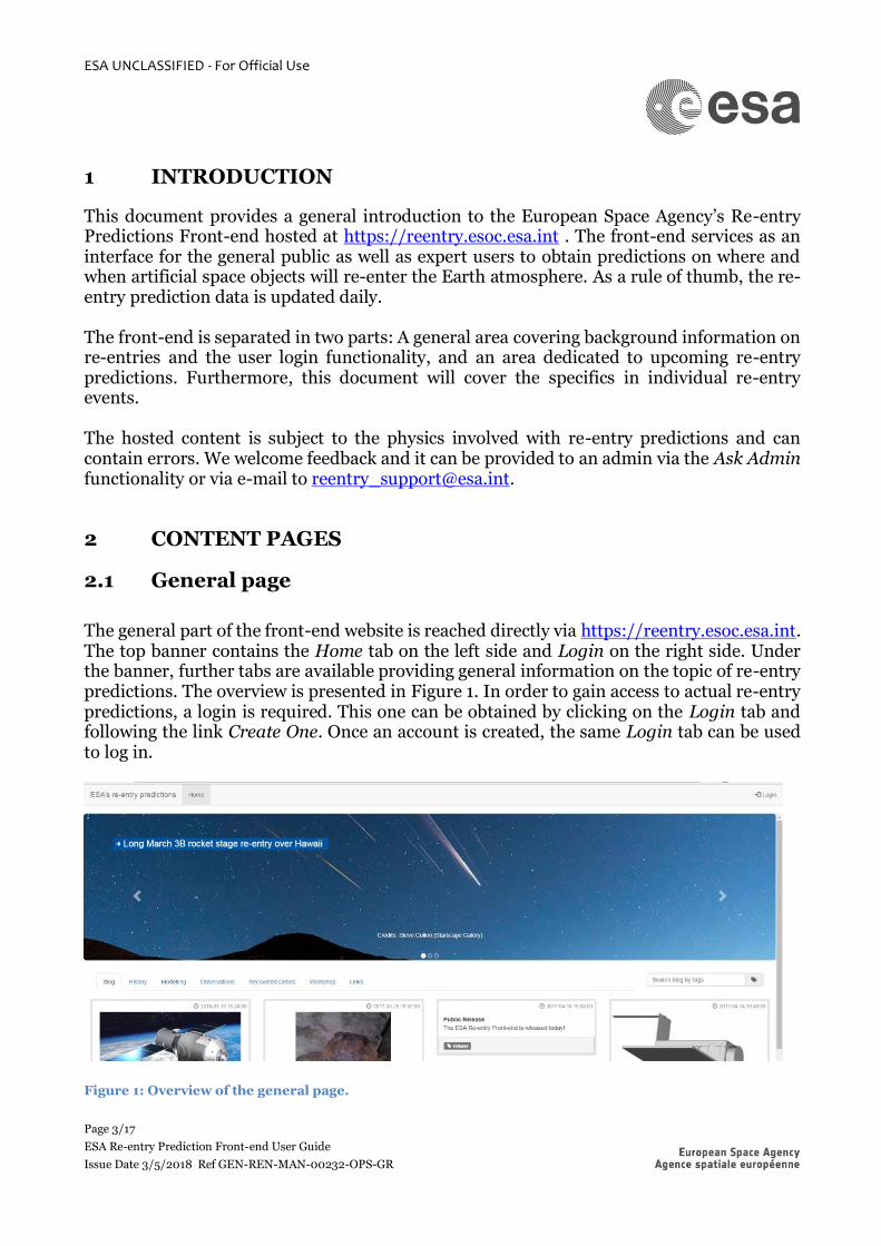
The general part of the front-end website is reached directly via https://reentry.esoc.esa.int. The top banner contains the Home tab on the left side and Login on the right side. Under the banner, further tabs are available providing general information on the topic of re-entry predictions. The overview is presented in Figure 1. In order to gain access to actual re-entry predictions, a login is required. This one can be obtained by clicking on the Login tab and following the link Create One. Once an account is created, the same Login tab can be used to log in.

Figure 1: Overview of the general page.

https://reentry.esoc.esa.int/

mailto:[email protected]

https://reentry.esoc.esa.int/


/17



2.2 Re-entry Predictions page

After successfully logging in as described in 2.1, a second tab called Re-entries will appear to right of the Home tab as shown in Figure 2. The Home tab will bring the user back to the general page, without logging out, whereas the Re-entries tab will bring you to a view on the upcoming re-entries. The page will allow the user to view the re-entries which took place during the past 60 days as well as the ones predicted to happen during the next 60 days. The data of single prediction, the most recent one, is shown here. Three ways of visualising the data, so called modes, are available: Table listing, Gantt chart, and World view. To switch between those, three buttons are available below the Login tab and show in Figure 3. In order to filter the data available in the three visualisation modes, a control panel is available on the left side of the pages. It allows to filter for Followed events, Cospar ID, SATNO, Name, predicted Re-entry Date, Mass range expressed in kilogram, object Class, current orbital Inclination expressed in degree, current orbital Perigee height expressed in kilometres, current orbital Apogee height expressed in kilometres, prediction Tool, and Country of origin. In the visualisation modes, information is provided on the predicted Re-entry Date rounded to the nearest day and prediction Uncertainty taken as ±20% of the remaining orbital lifetime, next to the filter values described below.

Figure 2: Overview of the general page after logging in.


/17



The filter list values are all reflected in the three visualisation modes. All hosted information is derived from the European Space agency’s DISCOS database. This database, which contains a more exhaustive list on object properties, can be access via https://discosweb.esoc.esa.int . An introduction to the object Class definition is available at https://discosweb.esoc.esa.int/web/guest/statistics . The COSPAR ID is understood as the object designator under the United Nations outer space treaty, the SATNO corresponds to the US catalogue number, and the prediction Tool category can be grouped based on propagation theory as follows: Analytic (FliP, ORBP), Semi-analytic (FOCUS2, FOC50), and Semi-analytic with numeric refinements (RAPID). An object with Mass 0.0 indicates that the information is not available from DISCOS. For objects in eccentric orbits, the uncertainty may be higher than the reported 20% of the remaining lifetime. Objects included in this list do not necessarily pose a significant on ground risk. General comments on the content of the data in the three visualisation modes can be send to an admin via the Ask Admin chat box below the filter control panel. In the Table listing visualisation mode, an Event button as highlighted in Figure 4 will bring the user into an event window where the history of the predictions is stored and retrievable. This page is described in 2.3.

Figure 3: Switch between re-entry visualisation modes.

Figure 4: Event button from the Table listing visualisation mode.

https://discosweb.esoc.esa.int/

https://discosweb.esoc.esa.int/web/guest/statistics


/17



2.3 Detail page

After entering on the detail page, as described in 2.2 , a new tab called Detail will be added next to the Re-entries tab on the top of the page. This tab contains the history of the past re-entry predictions for a single object. On the left side of the page, three different panel are available to control the visible information. The first panel, identified with the COSPAR ID and extendible with the small triangle, recaps the general event information. It also gives the opportunity to follow the event with the Star button. The middle panel contains access to the available history: A plot contained the re-entry prediction epoch with the associated uncertainty as function of the prediction epoch, also called creation epoch; a plot showing the apogee and perigee height information as function of the prediction epoch, also called creation epoch; and the tabulated prediction history used to create the aforementioned plots. Occasionally, object specific information can be distributed via this panel as well. Below the middle panel with the prediction histories, comments on the content of the data on this detailed page can be send to an admin via the Ask Admin chat box.

3 RESTRICTED ACCESS PAGES

Users or entities representing the interest of communities with a special focus on re-entries, e.g. civil protection agencies, can requires access to detailed re-entry predictions for objects of high interest. Request for such functionality would need to be addressed via e-mail to [email protected] and include a justification.

4 BASICS OF PREDICTING RE-ENTRY EVENTS

Re-entry predictions in general come down to the capacity of long- (years), mid- (a few weeks), and short-term (less than a day) orbit propagations and the ability to forecast the accompanying input parameters to the environment models. The first major perturbation factor for the orbit propagation is the non-spherical Earth, which as an enacted force that can be expressed by the harmonic expansion of a gravity potential field

𝑈 = −𝜇

𝑟(1 + ∑

𝐽�̃�𝑃𝑛0(sin 𝜃)

(𝑟𝑅

)𝑛

𝑁𝑧

𝑛=2

+ ∑ ∑𝑃𝑛

𝑚(sin 𝜃)(𝐶𝑛�̃� cos 𝑚𝜑 + 𝑆𝑛

�̃� sin 𝑚𝜑)

(𝑟𝑅

)𝑛

𝑛

𝑚=1

𝑁𝑡

𝑛=2

)

where 𝜇 is the standard gravitational parameter of the Earth, 𝑟, 𝜃, and 𝜑 are the geodetic coordinated of an object in the field, 𝑃𝑛

𝑚 are the Legendre polynomials and associated

Legendre functions, 𝑅 is the average Earth radius, and 𝐽�̃�, 𝐶𝑛�̃�, and 𝑆𝑛

�̃� are the normalised coefficients for the field expansion. The order of the gravity potential, i.e. n, has been empirically derived up to 2190 (GECO model, combining GOCE data and EGM2008), but for re-entry predictions models with orders below a 100 are generally sufficient, depending

mailto:[email protected]


/17



on the orbits under consideration. The same type of harmonic expansions can be made for the gravity potential fields of the Sun and Moon, which can have a strong impact on the re-entry predictions for orbits with a high eccentricity. However here an order of 1 is already sufficient for the vast majority of cases. This potential field can directly be used in the so-called Lagrange Perturbation Equations applied to Keplerian elements to derive the main effect from them. The first order effects are secular drifts over time in the line of ascending nodes Ω and line of apsides ω:

𝑑Ω

𝑑𝑡≈ −

3

2√

𝜇

𝑎3𝐽2 (

𝑎𝑒

𝑎)

2 1

(1 − 𝑒2)2cos 𝑖

𝑑ω

𝑑𝑡≈

4

3√

𝜇

𝑎3𝐽2 (

𝑎𝑒

𝑎)

2 1

(1 − 𝑒2)2(5 cos2 𝑖 − 1)

and periodic changes in the other components. Close to the re-entry, this can be used to derive the secular drift in geographic longitude of the ascending node

Δ𝑆Ω ≈ −21.8° − 0.6° cos 𝑖 . In general, the strength of the combination of the Lagrange Perturbation Equations and the potential expansion lies in the derivation of analytic and semi-analytic approximations for the motion of an object in the gravity field. In case of the perturbation by Sun and Moon, this requires approximating their orbits as well with analytical formulations. The strength of the individual perturbations is shown in Figure 5. A second major perturbation from the re-entry predictions point of view is due to the motion of the satellite through and atmosphere. This perturbation depends on the local atmospheric density 𝜌, the aerodynamic velocity with respect to the atmosphere (accounting for the Earth rotation and winds), the ratio of the projected cross-section 𝐴 in direction of the aerodynamic velocity to the mass 𝑚, and the aerodynamic coefficients of the spacecraft. For most orbital applications, including re-entry predictions, the aerodynamic coefficients are reduced to a drag and lift term, 𝑐𝐷 and 𝑐𝐿, which capture the resistance (drag) and generated lift of an object in a fluid. The later one is usually assumed to be 0, apart for analysis or re-entry vehicles in the lower layers of the atmosphere. To study the first order effects of this perturbation the Gauss Perturbation Equations, a reformulation of the general Lagrange perturbation equations, can be used. This results in secular drifts in semi-major axis 𝑎 and eccentricity 𝑒 over time:

𝑑𝑎

𝑑𝑡≈ −𝐵𝜌𝑝𝑒𝑎2

𝑛

2𝜋exp(−𝑧) (𝐼0(𝑧) + 2𝑒𝐼1(𝑧) +

4

3𝑒2(𝐼0(𝑧) + 𝐼2(𝑧)))

𝑑𝑒

𝑑𝑡≈ −𝐵𝜌𝑝𝑒𝑎(1 − 𝑒2)

𝑛

2𝜋exp(−𝑧) (𝐼1(𝑧) +

1

2𝑒(𝐼0(𝑧) + 𝐼2(𝑧)) +

1

8𝑒2(3𝐼1(𝑧) + 𝐼3(𝑧)))

𝐵 = 𝑐𝐷

𝐴

𝑚

𝑧 =𝑎𝑒

𝐻𝜌𝑝𝑒


/17



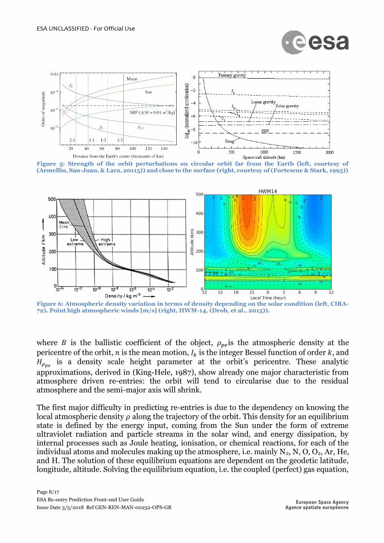
Figure 5: Strength of the orbit perturbations on circular orbit far from the Earth (left, courtesy of (Armellin, San-Juan, & Lara, 20115)) and close to the surface (right, courtesy of (Fortescue & Stark, 1995))

Figure 6: Atmospheric density variation in terms of density depending on the solar condition (left, CIRA-72). Point high atmospheric winds [m/s] (right, HWM-14, (Drob, et al., 2015)).

where 𝐵 is the ballistic coefficient of the object, 𝜌𝑝𝑒is the atmospheric density at the

pericentre of the orbit, 𝑛 is the mean motion, 𝐼𝑘 is the integer Bessel function of order 𝑘, and 𝐻𝜌𝑝𝑒

is a density scale height parameter at the orbit’s pericentre. These analytic

approximations, derived in (King-Hele, 1987), show already one major characteristic from atmosphere driven re-entries: the orbit will tend to circularise due to the residual atmosphere and the semi-major axis will shrink. The first major difficulty in predicting re-entries is due to the dependency on knowing the local atmospheric density 𝜌 along the trajectory of the orbit. This density for an equilibrium state is defined by the energy input, coming from the Sun under the form of extreme ultraviolet radiation and particle streams in the solar wind, and energy dissipation, by internal processes such as Joule heating, ionisation, or chemical reactions, for each of the individual atoms and molecules making up the atmosphere, i.e. mainly N2, N, O, O2, Ar, He, and H. The solution of these equilibrium equations are dependent on the geodetic latitude, longitude, altitude. Solving the equilibrium equation, i.e. the coupled (perfect) gas equation,


/17



hydrostatic equation under the gravity field, and the diffusive thermal equilibrium equation, is one issue, but accurately modelling the input for the Sun is another one. In reality, only proxies can be used to mimic the energy input. Often used proxies for this are the solar radio flux at 10.7 cm (2800 MHz), indicator of disturbances in the Earth's magnetic field as captured in the planetary K-index, or simply the Sun spot number which underlies both. These proxies are selected for our ability to measure them on Earth, not necessarily because they correlated best to the atmospheric physics. Moreover, they are notoriously difficult to forecast reliably for more than a few days. An overview of these influences are given in Figure 6 till Figure 8.

Figure 7: Five solar cycles of daily geomagnetic and solar activity observations.

Figure 8: One solar cycle of averaged geomagnetic and solar activity observations and one cycle forecast.


/17



Given the complexity of these dynamics, a multitude of atmosphere models have been developed. An excellent overview is presented in (Vallado & Finkleman, 2008), and the consequences on a real case are demonstrated in Figure 9. ESA’s GOCE (Gravity field & steady-state Ocean Circulation Explorer) was launched on 17th March 2009, from Plesetsk (Russia), on a Rokot (SL-19), into an initial Sun synchronous orbit with perigee altitude of 272 km, apogee at 290 km, and inclination of 96.71 degree. After more than 4 years of successful operations, the drag-compensation ion propulsion reached fuel depletion as expected. The altitude of GOCE resulted in a remaining orbital lifetime until re-entry into the atmosphere of less than a month. During this re-entry, the satellite continued registering acceleration, allowing us to reconstruct the atmospheric environment around the satellite and we can use it to compare to the current state of the art prediction models: NRLMSIS-00, JB2008, DTM-2013 (all three semi-empirical), and WACOMM-X (a physics-based model). This indicated a significant difference between all four models as compared among themselves and to the observations. Next to difficulties in forecasting 𝜌, also the ballistic coefficient 𝑐𝐷 𝐴 𝑚⁄ is not trivial to use in practical predictions. In Figure 10 the project cross-section, 𝐴, for a non-convex example satellite is given while parametrically varying the view angle, i.e. under the assumption of different attitude motions. This can lead to huge variations in this value. Similarly, the mass

Figure 9: Atmosphere model comparison on the trajectory of the GOCE re-entry, in relation to the atmospheric densities derived from the satellite itself (Courtesy of Eelco Doornbos TUDelft / ESA).


/17



Figure 10: Projected cross-section estimation over different viewing angles for ESA's ERS-2 satellite (top) and A*Cd variations for ESA’s GOCE satellite depending on the atmospheric drag at loss of control (bottom) (ESA, ESA-DRAMA).

𝑚 is difficult to estimate in practice, e.g. due to uncertainties on the propellant on-board a spacecraft. The drag coefficient 𝑐𝐷 depends on the shape, material, the speed-ratio, the temperature, and the flow regime, e.g. Figure 11. The flow field can be capture by three main numbers:

• The Mach number, which is the ration of the local flow velocity to the speed of sound of the medium. This captures the ratio of kinetic energy to internal energy of the flow. Hypersonic velocities are generally considered to have Mach number 5 or above, but are shape and material dependent.

• The Reynolds number, which is the ratio of the product of the local density with local flow velocity with the object’s reference length to the dynamic viscosity term of the medium. This captures the ratio of pressure forces to viscous forces. Low Reynolds number flow as called laminar, leading to smooth motion of the medium. High Reynolds number are called turbulent, characterised by instabilities in the flow.

4

6

8

10

12

14

16

0 10 20 30 40 50 60

Are

a*C

d p

er

revo

lutio

n

propagation time [h]

drag 106.0 mN, alt 168.0 km










/17



• The Knudsen number, which is the ratio of the mean free path length to the characteristic length of the object. This captures the interaction of the particles of the flow with the object. Flows with Knudsen numbers above 10 are generally considered as within the free molecular regime, Knudsen numbers below 0.01 as the continuum flow regime, with the transition or rarefied regime in between.

As the ballistic coefficient is difficult to derive for any given object and moreover variable, e.g. it can be done in the frame of precise orbit determination for navigation or scientific satellites, alternatively it is often estimated as part of space surveillance processes. The ballistic coefficient is often a by-product from orbit determination procedure to fit the observed orbit decay during the data gathering period. Without directly using observations but when ephemerides are available instead, the ballistic coefficient can be estimated by using a time series of semi-major axis values:

1. The initial estimate for 𝐵 is obtained by back-propagating the final state of the window to match the first state;

2. And iterate on 𝐵 to minimise the residuals for all the intermediate values of the semi-major axis in the time series.

Figure 11: Drag coefficients estimated based on the object shape and orbit altitude based Sentman's model (top, (Moe & Moe, 2005)). Drag coefficient evolution for a sphere in function of the flow field as defined by the Knudsen number (bottom).


/17



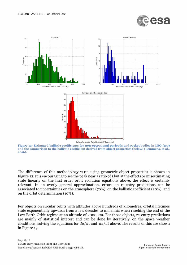
Figure 12: Estimated ballistic coefficients for non-operational payloads and rocket bodies in LEO (top) and the comparison to the ballistic coefficient derived from object properties (below) (Lemmens, et al., 2016).

The difference of this methodology w.r.t. using geometric object properties is shown in Figure 12. It is encouraging to see the peak near a ratio of 1 but at the effects or misestimating scale linearly on the first order orbit evolution equations above, the effect is certainly relevant. In an overly general approximation, errors on re-entry predictions can be associated to uncertainties on the atmosphere (70%), on the ballistic coefficient (20%), and on the orbit determination (10%). For objects on circular orbits with altitudes above hundreds of kilometres, orbital lifetimes scale exponentially upwards from a few decades to millennia when reaching the end of the Low Earth Orbit regime at an altitude of 2000 km. For those objects, re-entry predictions are mainly of statistical interest and can be done by iteratively, on the space weather conditions, solving the equations for 𝑑𝑎 𝑑𝑡⁄ and 𝑑𝑒 𝑑𝑡⁄ above. The results of this are shown in Figure 13.


/17



Figure 13: Long term orbital lifetimes versus perigee height for non-maneuvering object on circular LEOs (Lemmens, et al., 2016).

Figure 14: Relative prediction error sample for object between 2014 and 2016 when using single averaged theory alone (left) or using full numerical propagation when the orbit is below 200km altitude (right) (Lemmens, et al., 2016).

To automatically monitor and forecast the orbit evolution of a re-entering object over periods of several years to a few weeks of remaining lifetime, i.e. less than a few solar cycles, computationally efficient yet sufficiently accurate methods must be applied. For this purpose, ESA uses a propagator called Fast Orbit Computation Utility Software (FOCUS) (Klinkrad, 2006). The propagator integrates the combined time rates of change of singly averaged perturbation equations, taking into account a non-spherical Earth gravity potential, a dynamic Earth atmosphere, lunisolar gravity perturbations, and solar radiation pressure in combination with an oblate, cylindrical Earth shadow. The single averaging refers to averaging the osculating orbital elements over a fast variable, in this case the mean anomaly. Coping with complex atmospheric density and wind models while aiming for computational speed is done by numerical Gauss quadrature of the mean rates of change of the singly averaged elements, and afterwards numerical integration of the combined equations. Near re-entry, i.e. during the last few weeks, the approximations made by using single average values and the numerical quadrature lose their accuracy. In general, a hand-over to a full numerical integrator (with associated time penalty) is done when the perigee altitude of the orbit reaches 200km.


/17



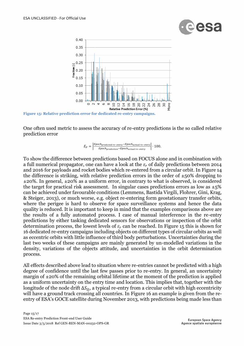
Figure 15: Relative prediction error for dedicated re-entry campaigns.

One often used metric to assess the accuracy of re-entry predictions is the so called relative prediction error

𝐸𝑃 = |𝐸𝑝𝑜𝑐ℎ𝑝𝑟𝑒𝑑𝑖𝑐𝑡𝑒𝑑 𝑟𝑒−𝑒𝑛𝑡𝑟𝑦−𝐸𝑝𝑜𝑐ℎ𝑎𝑐𝑡𝑢𝑎𝑙 𝑟𝑒−𝑒𝑛𝑡𝑟𝑦

𝐸𝑝𝑜𝑐ℎ𝑝𝑟𝑒𝑑𝑖𝑐𝑡𝑖𝑜𝑛−𝐸𝑝𝑜𝑐ℎ𝑎𝑐𝑡𝑢𝑎𝑙 𝑟𝑒−𝑒𝑛𝑡𝑟𝑦| ∙ 100.

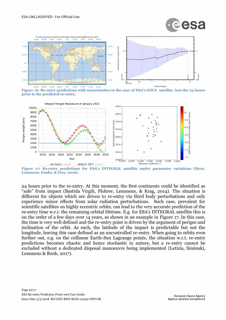
To show the difference between predictions based on FOCUS alone and in combination with a full numerical propagator, one can have a look at the 𝐸𝑃 of daily predictions between 2014 and 2016 for payloads and rocket bodies which re-entered from a circular orbit. In Figure 14 the difference is striking, with relative prediction errors in the order of ±50% dropping to ±20%. In general, ±20% as a uniform error, in contrary to what is observed, is considered the target for practical risk assessment. In singular cases predictions errors as low as ±5% can be achieved under favourable conditions (Lemmens, Bastida Virgili, Flohrer, Gini, Krag, & Steiger, 2013), or much worse, e.g. object re-entering form geostationary transfer orbits, where the perigee is hard to observe for space surveillance systems and hence the data quality is reduced. It is important to keep in mind that the examples comparisons above are the results of a fully automated process. I case of manual interference in the re-entry predictions by either tasking dedicated sensors for observations or inspection of the orbit determination process, the lowest levels of 𝐸𝑃 can be reached. In Figure 15 this is shown for 16 dedicated re-entry campaigns including objects on different types of circular orbits as well as eccentric orbits with little influence of third body perturbations. Uncertainties during the last two weeks of these campaigns are mainly generated by un-modelled variations in the density, variations of the objects attitude, and uncertainties in the orbit determination process. All effects described above lead to situation where re-entries cannot be predicted with a high degree of confidence until the last few passes prior to re-entry. In general, an uncertainty margin of ±20% of the remaining orbital lifetime at the moment of the prediction is applied as a uniform uncertainty on the entry time and location. This implies that, together with the longitude of the node drift Δ𝑆Ω, a typical re-entry from a circular orbit with high eccentricity will have a ground track crossing all countries. In Figure 16 an example is given from the re-entry of ESA’s GOCE satellite during November 2013, with predictions being made less than


/17



Figure 16: Re-entry predictions with uncertainties in the case of ESA's GOCE satellite, less the 24 hours prior to the predicted re-entry.

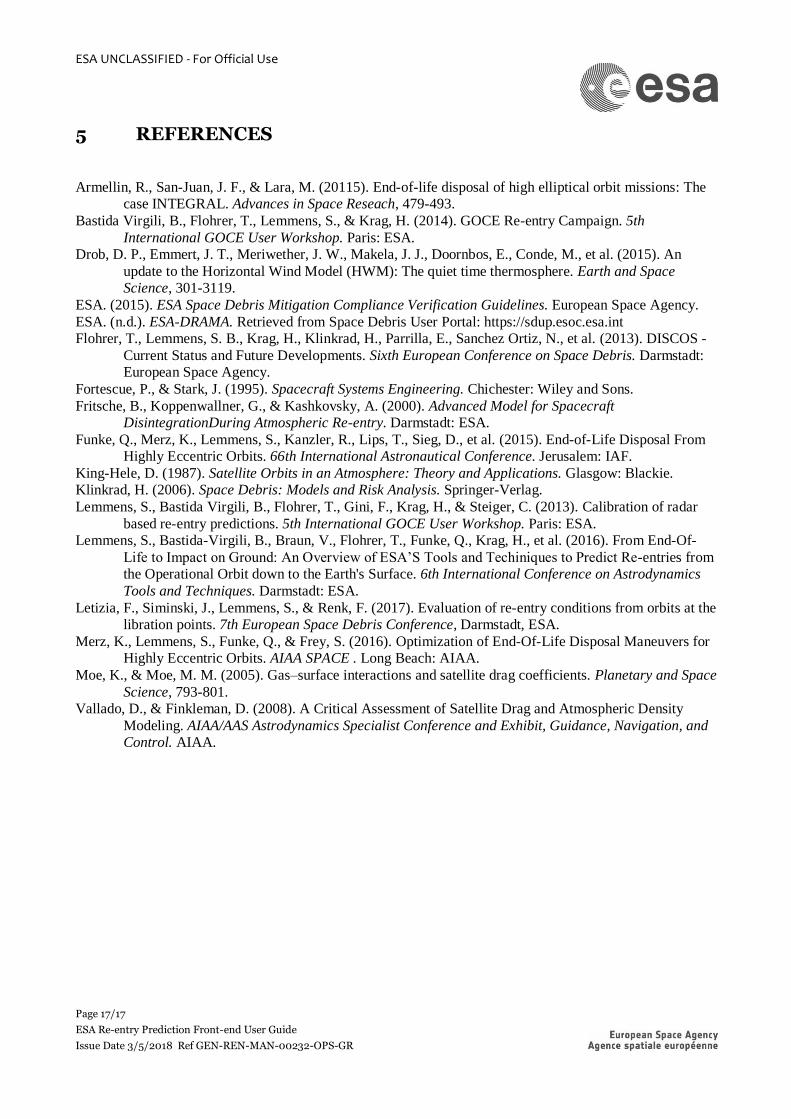
Figure 17: Re-entry predictions for ESA's INTEGRAL satellite under parameter variations (Merz, Lemmens, Funke, & Frey, 2016).

24 hours prior to the re-entry. At this moment, the first continents could be identified as “safe” from impact (Bastida Virgili, Flohrer, Lemmens, & Krag, 2014). The situation is different for objects which are driven to re-entry via third body perturbations and only experience minor effects from solar radiation perturbations. Such case, prevalent for scientific satellites on highly eccentric orbits, can lead to the very accurate prediction of the re-entry time w.r.t. the remaining orbital lifetime. E.g. for ESA’s INTEGRAL satellite this is on the order of a few days over 14 years, as shown in an example in Figure 17. In this case, the time is very well defined and the re-entry point is driven by the argument of perigee and inclination of the orbit. As such, the latitude of the impact is predictable but not the longitude, leaving this case defined as an uncontrolled re-entry. When going to orbits even further out, e.g. on the collinear Earth-Sun Lagrange points, the situation w.r.t. re-entry predictions becomes chaotic and hence stochastic in nature, but a re-entry cannot be excluded without a dedicated disposal manoeuvre being implemented (Letizia, Siminski, Lemmens & Renk, 2017).


/17



5 REFERENCES

Armellin, R., San-Juan, J. F., & Lara, M. (20115). End-of-life disposal of high elliptical orbit missions: The

case INTEGRAL. Advances in Space Reseach, 479-493.

Bastida Virgili, B., Flohrer, T., Lemmens, S., & Krag, H. (2014). GOCE Re-entry Campaign. 5th

International GOCE User Workshop. Paris: ESA.

Drob, D. P., Emmert, J. T., Meriwether, J. W., Makela, J. J., Doornbos, E., Conde, M., et al. (2015). An

update to the Horizontal Wind Model (HWM): The quiet time thermosphere. Earth and Space

Science, 301-3119.

ESA. (2015). ESA Space Debris Mitigation Compliance Verification Guidelines. European Space Agency.

ESA. (n.d.). ESA-DRAMA. Retrieved from Space Debris User Portal: https://sdup.esoc.esa.int

Flohrer, T., Lemmens, S. B., Krag, H., Klinkrad, H., Parrilla, E., Sanchez Ortiz, N., et al. (2013). DISCOS -

Current Status and Future Developments. Sixth European Conference on Space Debris. Darmstadt:

European Space Agency.

Fortescue, P., & Stark, J. (1995). Spacecraft Systems Engineering. Chichester: Wiley and Sons.

Fritsche, B., Koppenwallner, G., & Kashkovsky, A. (2000). Advanced Model for Spacecraft DisintegrationDuring Atmospheric Re-entry. Darmstadt: ESA.

Funke, Q., Merz, K., Lemmens, S., Kanzler, R., Lips, T., Sieg, D., et al. (2015). End-of-Life Disposal From

Highly Eccentric Orbits. 66th International Astronautical Conference. Jerusalem: IAF.

King-Hele, D. (1987). Satellite Orbits in an Atmosphere: Theory and Applications. Glasgow: Blackie.

Klinkrad, H. (2006). Space Debris: Models and Risk Analysis. Springer-Verlag.

Lemmens, S., Bastida Virgili, B., Flohrer, T., Gini, F., Krag, H., & Steiger, C. (2013). Calibration of radar

based re-entry predictions. 5th International GOCE User Workshop. Paris: ESA.

Lemmens, S., Bastida-Virgili, B., Braun, V., Flohrer, T., Funke, Q., Krag, H., et al. (2016). From End-Of-

Life to Impact on Ground: An Overview of ESA’S Tools and Techiniques to Predict Re-entries from

the Operational Orbit down to the Earth's Surface. 6th International Conference on Astrodynamics

Tools and Techniques. Darmstadt: ESA.

Letizia, F., Siminski, J., Lemmens, S., & Renk, F. (2017). Evaluation of re-entry conditions from orbits at the

libration points. 7th European Space Debris Conference, Darmstadt, ESA.

Merz, K., Lemmens, S., Funke, Q., & Frey, S. (2016). Optimization of End-Of-Life Disposal Maneuvers for

Highly Eccentric Orbits. AIAA SPACE . Long Beach: AIAA.

Moe, K., & Moe, M. M. (2005). Gas–surface interactions and satellite drag coefficients. Planetary and Space

Science, 793-801.

Vallado, D., & Finkleman, D. (2008). A Critical Assessment of Satellite Drag and Atmospheric Density

Modeling. AIAA/AAS Astrodynamics Specialist Conference and Exhibit, Guidance, Navigation, and

Control. AIAA.

manual / user guide / handbook - reentry.esoc.esa.int · handbook esa re-entry ... after...

Documents