manufacturing growth and local multipliers in china

Manufacturing Growth and Local Multipliers in China

Ting Wang and Areendam Chanda∗

First Draft: January 2017This Draft: June, 2017

Abstract

We study the impact of employment growth in manufacturing on job creation in thenon-tradable sector for prefecture-level cities in China. Using the 2000 and 2010 Cen-suses of Population, we apply the shift-share approach to isolate the exogenous changeof employment growth in manufacturing. For every hundred new manufacturing jobs,we find that 34 additional jobs are created in the non-tradable sector. We also showthat the effect is heterogeneous along a number of dimensions. More specifically, onenew job in high-technology manufacturing creates more jobs in the non-tradable sectorwhile low-technology manufacturing employment growth has no significant multipliereffect. Among the non-tradable industries, the multiplier is the largest for wholesale,retail, and catering. Finally, the effect is also geographically heterogeneous, with themultiplier being greater for inland regions.

JEL-Classification: O14; O18; R11; N95Keywords: Structural transformation; Local labor markets; Regional spillovers; China

∗Wang: Department of Economics, Louisiana State University, Baton Rouge, LA 70803, USA. Emailaddress: [email protected]. Chanda: Department of Economics, Louisiana State University, Baton Rouge,LA 70803, USA. Email address: [email protected]. We thank Ozkan Eren, Fang Yang, Bulent Unel,Seunghwa Rho, Naci Mocan, Dachao Ruan, Han Yu, Kui-Wai Li, Hao Guo, Phanindra Goyari, Scott Rozelle,Binzhen Wu, Di Mo, participants at the 2015 SEA Conference in New Orleans, and seminar participants atREAP-FSI (Stanford) and LSU for their comments. We are responsible for all errors.

1

1 Introduction

China’s structural transformation accompanied by its remarkable manufacturing based growth

is well known. This extraordinary growth is also reflected in China’s dominance in the global

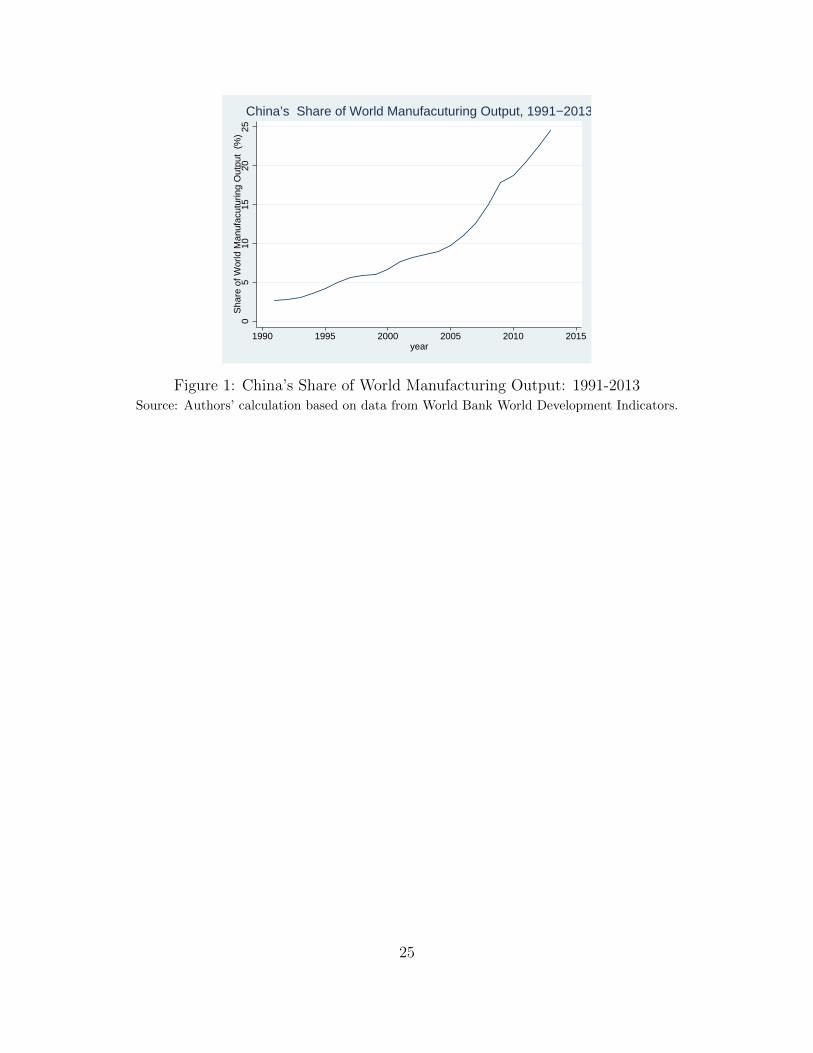
sphere. As shown in Figure 1, in 1991, China’s share of value-added in global manufacturing

was only 2.7%. It started to rise in the early 1990s, but increased radically since 2000, aided

by China’s accession to the WTO in 2002. By 2013, China’s share of world manufacturing

output reached 24.5%. During the first decade of the twenty first century manufacturing

employment increased from 44 million to 84 million.1

In this paper, we investigate the extent to which such rapid manufacturing growth in

China led to regional employment effects in the non-tradable sector. The importance of

manufacturing in the context of place based policies, and employment creation in particular,

has been extensively investigated in the literature.2 In addition to the direct absorption of

labor, the manufacturing sector can create jobs in other sectors through various channels.

First, services like finance, transportation, and information technology contribute to the

production process as intermediate inputs in the manufacturing sector. These productive

linkages lead to new jobs in these sectors when manufacturing grows. Second, increased

labor demand in manufacturing raises wages as long as labor supply is not perfectly elastic.

Higher wages, therefore, increase spending on local services like haircuts, restaurants, health

care, etc. This income-induced demand for local services also begets new jobs in the service

sector. The extraordinary growth of manufacturing in China during the first decade of the

twenty first century provides a natural setting to investigate the extent of these multiplier

effects.

In order to estimate these effects, we rely on a reduced form specification introduced

by Moretti (2010). He investigates the impact of employment in the tradable sector on

the non-tradable sector in the U.S. during 1980-2000.3 Ordinary least squares estimation

leads to inconsistent estimates if other factors affect employment in both manufacturing and

non-tradable sectors. To deal with endogeneity, Moretti employs an instrumental variable

constructed based on the shift-share approach (McGuire and Bartik, 1992) to isolate sources

of exogenous variation in manufacturing employment growth. The instrumental variable is

1Data are derived from China Industrial Economy Statistical Yearbooks. It covers state-owned andnon-state owned firms with annual sales above 5 million RMB.

2For a review of place based policies, see Kline and Moretti (2014) and for the role of manufacturing inemployment creation see Bivens (2003); Moretti (2010); Park and Chan (1989); Valadkhani (2005).

3Moretti (2010) defines manufacturing as the tradable sector. In this paper, we will use manufacturingand tradable interchangeably.

2

the manufacturing employment growth that would have occurred had employment grown at

the national growth rate. It captures the manufacturing employment growth caused only

by national shocks, purging local endogenous factors that affect employment. We apply the

analysis to China, taking into account its demographic and institutional characteristics.

More specifically, we use the 2000 and 2010 Censuses of Population to examine how

many jobs in the non-tradable sector (utility, construction, and services) are created when

one job is created in manufacturing for prefecture-level cities in China. Our choices of

data and research period are dictated largely by consideration of data quality. Population

censuses are preferred because they provide complete employment data in China. Using

employment data from other sources like City Statistical Yearbooks underestimates the size

of employment by omitting many self-employed workers (Li and Gibson, 2015). We focus on

the period from 2000 to 2010 because the population census in China began using the same

standard to aggregate data since 2000. 4

Our IV estimate suggests that for every ten jobs created in manufacturing, 3.4 additional

jobs are created in the non-tradable sector. Moreover, about 12.6% of employment growth

in the non-tradable sector can be attributed to employment growth in manufacturing.5 The

average multiplier effect remains robust after considering the potential effects of development

in neighboring areas, access to the world market, and physical geographical characteristics.

We conduct a falsification test to show the effect is not driven by some long-run common

causal factors that affect employment in both sectors. We also reconstruct the manufacturing

sector by excluding tobacco, and petroleum processing and coking. These two industries are

dominated by state-owned enterprises (SOEs), with shares of output exceeding 50% in 2010.

We find that SOEs in manufacturing do not drive our results.

We further investigate heterogeneous effects of the multiplier along different dimensions.

First, by looking at the effect of high- and low- technology manufacturing employment

growth, we find that high-technology employment creates jobs in the non-tradable sector,

while low-technology ones do not generate additional jobs. Second, examining the multiplier

for each non-tradable industry shows that the multiplier effect is the largest in wholesale,

4The aggregate employment data at the city level in 1990 Census of Population included all workers whostayed in the city for more than one year at the time of the census. In 2000 and 2010 Censuses of Population,employment data were collected from 10% of households, and the aggregate employment data at city levelincluded workers who stayed in the city for more than six months at the time of the census. Employmentdata from Population Census 1990 are not comparable to that from 2000 and 2010 Censuses of Population.

5One concern is whether utility, construction and services can be treated as non-tradable. Due to datalimitations, we cannot further classify their tradability. Instead, in a later part of the paper, we examine themultipliers for different non-tradable industries to show the heterogeneity of the multipliers.

3

retail and catering. Third, we study the multiplier effect across regions. During the earlier

reform period, the central government designed preferential policies to develop industrial

clusters at coastal cities, mainly relying on location advantages (Zheng et al., 2014). However,

industrial agglomeration in coastal cities began to decline since the mid-2000s. The decline

is due to rising land and labor cost in coastal cities (Li et al., 2012), and favorable investment

policies provided by inland governments (Zheng et al., 2014). Indeed, our result suggests a

smaller multiplier effect in coastal cities.

1.1 Related Literature

Our paper makes a contribution to two important strands of research - that of estimating

employment multipliers across time and space, and secondly, the literature on local economic

growth in China. With regards to the first, in addition to the United States, this approach

has been applied to estimate the employment multiplier effects in England (Faggio and

Overman, 2014), Italy (de Blasio and Menon, 2011), Sweden(Moretti and Thulin, 2013),

and OECD countries (van Dijk, 2014). To place our results in context, Moretti (2010) finds

that one new job in the manufacturing sector in the U.S. created 1.6 additional jobs in the

non-tradable sector during 1980-2000. van Dijk (2017), making finer classifications on the

extent of tradability of services, shows that this is an upper bound. Compared to the US,

studies have generally found the multiplier to be much lower in European countries. Moretti

and Thulin (2013) find the multiplier is 0.48 in Sweden during 1995-2007 while Faggio and

Overman (2014) show that the effect is negative for UK indicating that manufacturing growth

crowds out private services for the period 1999-2007. In similar vein, de Blasio and Menon

(2011) find that the multiplier is zero in Italy during 1991-2007. The authors attribute

the small or negative effects to limited labor mobility compared to the US which in turn

can be attributed to other frictions such as restrictions on housing supply or labor market

regulations. All of these countries are, of course, developed economies. Our estimates for

China are lower than that of the US but higher than that of the Europe. As in Europe, a host

of restrictions might be one reason why the multiplier is lower. China regulates non-tradable

sectors like utility, transportation, and finance. Also, the local government’s regulation of

land supply restricts construction, thereby restricting labor demand. Finally, even though

labor supply in China is certainly more elastic, the Hukou system prevents it from reaching

its full potential.

Another set of reasons could arise from the fact that China is a middle income country,

and hence at a different stage of development. First, Chinese manufacturing may not

4

outsource service oriented support activities to the same extent as firms in industrialized

nations. Thus while job creation in manufacturing might be larger, the linkage effect might

be lower. Second, lower wages usually means that a smaller fraction of income is dedicated

to consumption of services. Both of these factors may lower the magnitude of the multiplier.

However, being a labor intensive economy, it is also possible that the multiplier could be

larger since non-tradables will be more labor intensive. While, we are unable to disentangle

these various effects, it is not surprising that the effects are larger than Europe but lower

than the US.

Our paper also contributes to the literature on local growth in China. More specifically,

there is now a large body of research examining the effect of exports and FDI growth in

Chinese provinces and cities. Examples of the latter that are closely tied to our research

is the impact of of SEZ’s on local growth by Wang (2013) and Alder et al. (2016). Both

of these papers show that the introduction of SEZ’s have led to higher exports, foreign

direct investments, and per capita incomes. While we do not explicitly focus on SEZ’s,

our paper complements this line of research by capturing the local employment effects of

manufacturing growth. There is also a large literature that studies the labor markets and

local economic growth in China, particularly in connection with the Hukou system (e.g.

Bosker et al. (2012)). Most closely related to our research is a recent paper by Imbert et al.

(2016) which assesses the impact of labor migration from rural areas on wages in skilled and

unskilled industries at the firm level. Using rainfall and international crop price shocks to

isolate exogenous sources of migration from rural areas, they show that it depresses urban

wages, particularly of the less educated and also increases firm profits. By emphasizing a

demand driven effect on employment in urban areas, our research complements their focus

on supply driven factors.

In Section 2 we provide a brief description of the dataset. Section 3 describes the empirical

strategy. In Section 4, we report our main results. Section 5 concludes.

2 Data

The main variable of interest is the employment change in different industries at the local

level from 2000 to 2010. In this section, we briefly provide some background regarding the

definitions and construction of administrative regions and industrial classification system.

5

2.1 An Overview of Administrative Regions in China

China’s administrative divisions comprise of five levels. At the broadest level, the country

is divided into 27 provinces and four province-level municipalities.6 Second is the prefecture

level. It includes prefecture-level cities (dijishi), prefectures (diqu), leagues (meng) and

autonomous prefectures (zizhizhou).7 Third is the county level, including districts (qu),

county-level cities (xianjishi), and counties (xian). Fourth is the township (zhen) level. Fifth

is the village (cun) level.

The unit of analysis in this paper is a prefecture-level city. A prefecture-level city consists

of districts (qu), counties (xian), and county-level cities (xianjishi). The districts within a

prefecture-level city form an urban core area (shixiaqu), which is usually more industrialized

than the rest, and is the nearest Chinese analog to a standard city like a U.S. metropolitan

area ((Alder et al., 2016), (Baum-Snow et al., 2013)). The government of a prefecture-level

city is responsible for the economic development within its administrative region, leading

the administrative affairs of the urban core area, and governance of counties and county-

level cities. We focus on prefecture-level cities for two main reasons. First, manufacturing

activities could take place either in the urban core area or outside the urban core area.

The urban core area benefits firms through its better infrastructure and market access,

the agglomeration advantages from technological externalities (Duranton, 2007) and labor

market pooling (Breinlich, Ottaviano, and Temple, Breinlich et al.). The remaining areas,

instead, benefit firms via lower labor and land costs. Baum-Snow et al. (2013) find that

radial railroads have decentralized industrial activities in China. Investigating the whole

prefecture-level city, therefore, provides an average multiplier at the local level. Second,

both one- and two-digit employment data are available for prefecture-level cities, which

allows us to examine narrower industries.

Due to administrative reforms between 2000 and 2010, the prefecture-level cities reported

in the censuses of 2000 and 2010 are not identical. In Appendix A.1 we discuss details about

the adjustments made to construct comparable prefecture-level cities. The final sample

includes 277 prefecture-level cities, covering 91.6% of total population at the prefecture

level.

It is important to reiterate that the unit of analysis in this paper is based on administra-

6 A provincial-level municipality is a “city” with “provincial” power. The four province-level municipalitiesare Beijing, Tianjin, Shanghai and Chongqing.

7 A prefecture-level city is administered by a province. Prefectures used to be the most common divisionat the prefecture level, but have gradually converted to prefecture-level cities since 1983. Leagues andautonomous prefectures have more ethnic minorities.

6

tive divisions. China’s National Bureau of Statistics defines urban areas in the 2010 census

as areas located in or contiguous to the area where the local government is located (Chen

and Song, 2014). Although the definition is a bit different from that used in the 2000 census,

the difference is negligible (Chen and Song, 2014). As a result, a prefecture-level city may

include both urban (chengzhen) and rural (xiangcun) areas. For simplicity, we will refer to

the prefecture-level city as a city.

2.2 Data on Employment

As in Moretti (2010), the tradable sector is defined as manufacturing while the non-tradable

sector includes utilities, construction, and services. The aggregate employment in both trad-

able and non-tradable sectors are comparable across two censuses. However, employment in

sub-industries in the two censuses ares not perfectly comparable due to the different industry

classification systems. Take transportation as an example. Employment in transportation

reported in the 2010 Census included workers in public transportation like taxies and public

buses. However, employment of public transportation was included in social services in the

2000 Census. In order to compare employment changes for sub-industries, adjustments are

needed to construct comparable industries. We discuss the details in appendix A.2 and Table

A.1 lists the comparable industries from the two years. Further, we construct comparable

1-digit industries in the non-tradable sector. Appendix Table A.2 illustrates the classification

in the non-tradable sector.

3 Empirical Strategy and Results

Our primary focus is to investigate the causal relationship of employment growth in the

tradable sector on the non-tradable sector. Following Faggio and Overman (2014), total

employment growth in a city c between year t− τ and t can be written as

Ec,t − Ec,t−τEc,t−τ

=ENTc,t − ENT

c,t−τ

Ec,t−τ+ETc,t − ET

c,t−τ

Ec,t−τ+Eoc,t − Eo

c,t−τ

Ec,t−τ. (1)

Ec,t is the total employment in city c at time t. It includes employment in the non-tradable

sector (utilities, construction, and services) ENTc,t , employment in the tradable sector (manu-

facturing) ETc,t, and employment in other sectors (agriculture, mining, and governments jobs)

Eoc,t. (ENT

c,t −ENTc,t−τ )/(Ec,t−τ ) is the contribution of non-tradable sector to total employment

7

growth. (ETc,t − ET

c,t−τ )/(Ec,t−τ ) is the contribution of tradable sector to total employment

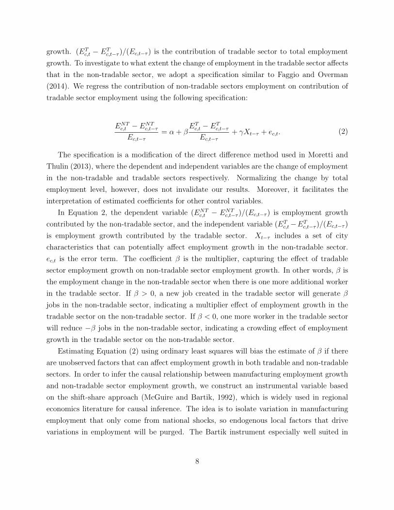
growth. To investigate to what extent the change of employment in the tradable sector affects

that in the non-tradable sector, we adopt a specification similar to Faggio and Overman

(2014). We regress the contribution of non-tradable sectors employment on contribution of

tradable sector employment using the following specification:

ENTc,t − ENT

c,t−τ

Ec,t−τ= α + β

ETc,t − ET

c,t−τ

Ec,t−τ+ γXt−τ + ec,t. (2)

The specification is a modification of the direct difference method used in Moretti and

Thulin (2013), where the dependent and independent variables are the change of employment

in the non-tradable and tradable sectors respectively. Normalizing the change by total

employment level, however, does not invalidate our results. Moreover, it facilitates the

interpretation of estimated coefficients for other control variables.

In Equation 2, the dependent variable (ENTc,t − ENT

c,t−τ )/(Ec,t−τ ) is employment growth

contributed by the non-tradable sector, and the independent variable (ETc,t−ET

c,t−τ )/(Ec,t−τ )

is employment growth contributed by the tradable sector. Xt−τ includes a set of city

characteristics that can potentially affect employment growth in the non-tradable sector.

ec,t is the error term. The coefficient β is the multiplier, capturing the effect of tradable

sector employment growth on non-tradable sector employment growth. In other words, β is

the employment change in the non-tradable sector when there is one more additional worker

in the tradable sector. If β > 0, a new job created in the tradable sector will generate β

jobs in the non-tradable sector, indicating a multiplier effect of employment growth in the

tradable sector on the non-tradable sector. If β < 0, one more worker in the tradable sector

will reduce −β jobs in the non-tradable sector, indicating a crowding effect of employment

growth in the tradable sector on the non-tradable sector.

Estimating Equation (2) using ordinary least squares will bias the estimate of β if there

are unobserved factors that can affect employment growth in both tradable and non-tradable

sectors. In order to infer the causal relationship between manufacturing employment growth

and non-tradable sector employment growth, we construct an instrumental variable based

on the shift-share approach (McGuire and Bartik, 1992), which is widely used in regional

economics literature for causal inference. The idea is to isolate variation in manufacturing

employment that only come from national shocks, so endogenous local factors that drive

variations in employment will be purged. The Bartik instrument especially well suited in

8

the context of China since the local economy in China is more likely to be affected by national

policies. More specifically, we use the national employment growth rate in manufacturing

and the initial share of manufacturing employment in the city to capture the exogenous

employment growth contributed by the manufacturing sector. The instrument is calculated

as:

ETc,t−τ

Ec,t−τ×ET

−c,t − ET−c,t−τ

ET−c,t−τ

, (3)

where (ET−c,t − ET

−c,t−τ )/(E−c,t−τ ) is the national growth rate of manufacturing employment

excluding city c. Although the national employment growth rate constructed for each city

is different, the main source of variance in the instruments is driven by the initial share of

manufacturing employment (Baum-Snow and Ferreira, 2014).

The validity of the instrument is subject to the critique that the initial share may correlate

with other factors which in turn affect non-tradable sector employment. To alleviate this

concern, we use a rich set of control variables capturing the starting period demographic and

labor composition that may affect employment at the city level. We control for the share

of urban hukou population in 2000. Hukou is the household registration system in China

that classifies people to agricultural (rural) and non-agricultural (urban) hukou.8 It has been

increasingly documented in the literature as a source of labor mobility restriction, undersized

cities, and unexploited gains from agglomeration (Au and Henderson, 2006; Bosker et al.,

2012). The share of urban population increased from 18% to 50% from 1978 to 2010, while

the share of urban hukou population increased from 16% to 34%. Controlling for the urban

hukou population share captures the original residence of the city’s labor force. The second

control variable is share of the population with college education above age 6 in 2000. It

captures human capital at the starting period, a common control variable in the urban and

regional growth literature (Glaeser et al., 2015)

We further include a region dummy variable indicating whether the city lies in coastal

provinces. Policies to develop industrial clusters targeted coastal areas at the beginning of

the reform period. As a result, the initial share of manufacturing employment is likely to

8Hukou was used to restrict rural-urban migration before 1978. Nowadays a person is free to move, butthe type of hukou determines the level of welfare to which is he entitled, including education, health care,and pension (Song, 2014). In addition, rural hukou can only be converted to urban hukou after meetingrequirements imposed by local governments such as holding a college degree, purchasing a local house, etc.(Chan and Buckingham, 2008).

9

be related to the region where the city is located. A city is assigned a region dummy taking

a value of 1 if it is in the coastal provinces of Hebei, Liaoning, Jiangsu, Zhejiang, Fujian,

Shandong, and Guangdong. We also use a dummy variable identifying whether a city is the

capital city of the province. Capital cities are usually more developed compared to others,

which may affect employment growth differently (Chanda and Ruan, 2017). To account

for the concern that employment growth may be correlated to city size, we control for the

log value of initial employment. In addition, the initial unemployment rate is also used to

capture labor surplus.9

Initial sectoral composition may affect subsequent employment growth. A city with an

initially higher share of non-tradable employment may experience slower growth in that

sector. A city with a larger government employment may demand more non-tradable goods,

inducing the growth of non-tradable employment. We add both the share of non-tradable

employment and share of government employment to control the potential effect of the initial

sectoral composition.

We perform robustness checks via several strategies. First, to consider spatial effects

we use additional controls such as a dummy taking a value of 1 if the city has a border

with one of the province-level municipalities, log average night light density from 1995 to

1999 in neighboring cities, and proximity to the nearest port city to capture the effects of

neighboring regions and access to world markets.10 Second, we add geographical controls

including temperature, rainfall, and altitude to show our results hold.11 Third, we conduct a

falsification test to show the result is not driven by some long-run common factors. Fourth,

to address the concern that the result may be driven by employment growth in SOEs, we

exclude tobacco, petroleum processing and coking from the manufacturing sector output

share of SOEs in both industries were above 50% in 2010.12

In the second part of the paper, we examine heterogeneous effects along a number of di-

mensions. First, we examine the multiplier effect of high- and low-technology manufacturing

industries. The details regarding the classification are introduced in Section 4. Following

9 Feng et al. (2015) document that official statistics understate Chinese unemployment rate. It is less ofa concern in this paper. Official unemployment rates only account for unemployed people with local hukou,but unemployment rates calculated from population census covers all people with and without local hukou.

10 Two cities are neighbors if they share a common border. Night lights data are from the NationalGeophysical Data Center. The distance to the nearest port city is the great circular distance calculated bygeodist in Stata.

11 Geographical data such as rainfall, temperature, and altitude are from Global Climate Data.12 We add the initial output share of SOE industries as a control variable, and the results remain robust.

10

Moretti (2010), we estimate a model,

ENTc,t − ENT

c,t−τ

Ec,t−τ= α + β1

ETHc,t − ETH

c,t−τ

Ec,t−τ+ β2

ETLc,t − ETL

c,t−τ

Ec,t−τ+ γXt−τ + ec,t, (4)

where ETHc,t and ETL

c,t are the employment in the high- and low-technology manufacturing

industries respectively. We use instruments constructed specific to each group to estimate

consistent β1 and β2. Second, we investigate the multiplier effect for each non-tradable

industry. Third, we investigate whether the multiplier effect varies with region. We interact

the tradable sector employment growth contribution with indicators of whether the city lies

in a coastal province.

3.1 Baseline Results

In Table 1 we present the descriptive statistics for 277 prefecture-level cities. From 2000

to 2010, the contributions of manufacturing and non-tradable sector to total employment

growth were 4.98% and 13.15% respectively. From 2000 to 2010, total employment grew by

6.58%. During this period, agricultural employment declined, with a negative contribution

(-11.9%) to employment growth. Of the 277 cities, 35% are located in coastal provinces, 9%

are capital cities, and 6.13% have a border with one of the four provincial municipalities.

We calculate the proximity to the nearest port city as the reciprocal of one plus distance in

thousands of kilometers.13 A value of 1 indicates the city has one of the biggest ports.

In Table 2, we present ordinary least squares estimates regressing the contribution of

non-tradable sector employment on the contribution of manufacturing employment. In

column (1), we control for initial demographic characteristics (initial shares of urban hukou

population and population with college education), region dummy, capital city dummy, log

value of initial employment, and unemployment rate. The point estimate implies that each

additional job in manufacturing creates 0.499 additional jobs in the non-tradable sector.

The coefficient of urban hukou population share is significantly negative, suggesting cities

with a greater share of urban hukou population experienced smaller increase in non-tradable

sector employment. This might seem counter-intuitive at first. If a city has greater urban

hukou population share, by definition it will have smaller share of rural labor and fewer rural

migrants.14 Combes et al. (2015) find that rural migrants complement rather than crowd

13We use the 10 biggest port cities in China - Shanghai, Shenzhen, Qingdao, Zhoushan, Xiamen, Yingkou,Guangzhou, Ningbo, Dalian, and Lianyungang.

14 Rural migrants are defined as people who stay in urban areas while holding a rural hukou.

11

out local urban hukou workers, mainly working in labor-intensive industries. Rural migrants

usually take jobs urban hukou workers don’t want to take (Meng, 2012; Zhao, 2000). As a

result, a city with a lower share of rural labor may experience slower employment growth

because less labor is available to work in low-end non-tradable industries. Alternatively the

negative sign may simply reflect higher costs of living.

The estimate for share of population with college education is significant and positive,

suggesting cities with initially higher human capital stock were associated with higher

contribution of the non-tradable sector to total employment growth. Although a city with a

greater share of urban hukou population has a higher proportion of college educated people,

the two variables measure different characteristics. The former captures the original residence

of the local population, while the latter captures human capital. Given the low level of college

attainment rates, most people with an urban hukou did not have a college education. Finally,

the coefficient of the region dummy is significantly negative, implying cities in coastal areas

are associated with smaller contribution of the non-tradable sector to total employment

growth.

In column (2), we add initial share of non-tradable employment as an additional control to

ensure that our main result is not picking up a structural convergence effect. The multiplier

estimate decreases only slightly. The estimate of initial non-tradable employment share is

significantly positive, suggesting that cities with more people working in the non-tradable

sector experience greater contribution of the non-tradable sector to total employment growth.

In column (3), we consider the effect of initial government employment on employment

growth in the non-tradable sector. The coefficient is significantly positive, indicating cities

with a greater share of government employment experience greater contribution of the non-

tradable sector to total employment growth. One explanation is that workers in government

are usually more educated and earn more than non-government workers, so more government

jobs will lead to increased demand in local non-tradable goods and services. Going forward,

we will use column (3) as our baseline model.

3.2 Instrumental Variable Estimation

Table 3 presents the IV estimates for the same three specifications as Table 2. The instru-

mental variable is constructed based on Equation 3. The first stage estimates are reported

in Appendix Table C.1. Column (0) displays a univariate regression of employment growth

on the instrument while the remaining columns correspond to the second stage regressions

in Table 3. The coefficient of the instrument is positive and significant at 1 percentage level

12

in each specification, suggesting local manufacturing employment growth closely correlates

to national manufacturing employment growth. The Kleibergen-Paap rk Wald F statistic

from weak identification test is reported in the last row. For each of the specifications, the

null of weak instrument is easily rejected. Column (3) in Table 3 is the baseline result. The

coefficient of manufacturing employment contribution is 0.339, suggesting that for every ten

jobs created in manufacturing, about 3.4 additional jobs are generated in the non-tradable

sector. In addition, the result indicates that about 12.6% of employment growth in the

non-tradable sector can be attributed to employment growth in manufacturing.15 For the

average multiplier estimated in this section, the IV estimate is about 1.3 jobs lower. Thus,

while different it is not dramatically different from that of the OLS specification. However,

when investigating the heterogeneous effects in the next section, we will see that there are

significant differences between OLS and IV estimates. Finally, the share of urban hukou

population, college population share, coastal dummy, and the initial share of employees in

government all retain their significance.

3.3 Robustness Tests

3.3.1 Spatial and Geographical Characteristics

Employment growth in a city may not only be affected by characteristics like demographic

composition, city size, and labor market conditions, but also influenced by other factors like

development in its neighboring areas, access to world markets, and physical geographical

advantages. We investigate these factors in Table 4. We first use controls including a

dummy variable identifying whether a city has a border with one of the four provincial

municipalities - Beijing, Shanghai, Chongqing and Tianjin, log level of night light density

in neighboring cities, and inverse distance to the nearest port city. The first two variables

intend to control for the effect of neighboring regions, while the last variable captures access

to world markets. We further control for geographic variables including rainfall, temperature

and altitude. The total number of observations drop to 276 since the city of Zhoushan does

not have neighboring cities and hence no nighttime light data.

Columns (1) and (2) in Table 4 are OLS estimates, and corresponding IV estimates are

in columns (3) and (4). Appendix Table C.2 shows the first stage estimates. The estimated

coefficients of the instrument variable are significant at 1 percent. The F statistic indicates

the null of weak identification continues to be rejected. In column (1) of Appendix Table C.2,

1512.6% is calculated by 4.89*0.339/13.15, where 4.89 is the mean of manufacturing contribution to totalemployment growth, and 13.15 is the mean of non-tradable sector contribution to total employment growth.

13

being located near a port city increases employment growth in manufacturing. However, the

effect disappears when further controlling for geographical characteristics. The estimated

coefficient of altitude is negative and significant at 1 percent level, showing that cities with

lower altitudes experience greater contribution by manufacturing to employment growth.

Sharing a border with one of the four provincial municipalities does not affect manufacturing

employment growth.

In columns (3) and (4) of Table 4, our estimates suggest that one additional job in

manufacturing increases non-tradable employment by between 0.38 to 0.39. The coefficients

of urban hukou population share, share of population with college education share, region

dummy, and government share dummy remain significant and have the same signs as the

baseline model. One exception is the unemployment rate, which becomes significant at

the 10 percent level after controlling for geographical characteristics, suggesting that cities

with a higher unemployment rate have greater employment growth in the non-tradable

sector. Adjacency to one of the four provincial municipalities increases contribution by

the non-tradable sector to employment growth - the estimate is significant at 10 percent.

The estimates of development in neighboring cities, proximity to the nearest port city, and

other geographical characteristics, are insignificant.

One might be concerned that province-specific features can affect employment in both

tradable and non-tradable sectors for cities within its jurisdiction. In Appendix Table C.3,

we address this concern by controlling for province fixed effects (instead of the coastal

region dummy). Columns (1) to (3) are fixed effects estimates, and columns (4) to (6) are

corresponding IV estimates. The observations in IV regressions drop by 1 because Xining

city, the only prefecture-level city in Qinghai province, is dropped. The F-statistics in the

first stage suggest the instrument is strong. The multiplier effect is 0.36 and significant at 5

percent.

The evidence above suggests that our results are robust after considering potential effects

from neighboring areas, access to the world market, physical geographical characteristics,

and province fixed effects. To mitigate problems related to endogeneity we have restricted

ourselves to geography variables and initial conditions. We also conducted additional regres-

sions which included contemporaneous changes in variables correlated with economic growth.

These included growth in fixed asset investment, FDI, government expenditures, and also

growth in wages. They are listed in Appendix Table C.4. Our estimates are robust though

all of these variables except FDI are significant.16

16We also controlled for log initial GDP per capita to further rule out any effects of convergence. The

14

3.3.2 Falsification Test

During the period that we study, both tradable and non-tradable sectors experienced a

secular rise. Despite including a large set of control variables, one concern for the analysis

is that some other unknown long-run common causal factors, such as trade or population

growth, may drive the increase in employment in both sectors. To verify that our result

captures the causal effect of manufacturing employment growth on employment in the non-

tradable sector, we conduct a falsification test by regressing past employment growth in

the non-tradable sector on future employment growth in manufacturing. We report our

results in Table 5. The variable of interest is contribution of manufacturing to employment

growth from 2010 to 2013. Column (1) reports OLS estimates for the baseline model. The

coefficient of future manufacturing employment growth contribution is insignificant. The

IV estimates of the baseline model are presented in column (4) of Table 5. However, the

instrument is weak; the F statistics from first stage is 3.5. Although the IV estimates are

not informative, the OLS estimates suggest little correlation between future manufacturing

employment growth and past employment growth in the non-tradable sector. This finding

can alleviate the concern that some long-run factors driving employment in both sectors

might overestimate the multiplier effect.17

3.3.3 Role of State Owned Enterprises (SOEs)

The growth of the Chinese economy has been accompanied by a dramatic transformation

of SOEs. In the late 1990s, a policy named “Grasp the Large, Let go of the Small” was

adopted for reforms in SOEs. Small SOEs were closed or privatized, large SOEs in strategic

sectors (such as infrastructure construction, oil, and utilities) were merged and formed large

conglomerates controlled either by central or local governments (Li et al., 2015; Hsieh and

Song, 2015). The large SOEs earn more profits because of their monopoly power and remain

dominant in the market. In 2010, output share of SOEs in both tobacco and petroleum

processing and coking exceeded 50%. One may be concerned that the multiplier effect might

be driven by employment growth in SOEs since their employees earn higher wages than

non-SOE employees, creating higher demand for non-tradable goods and services.

We investigate this concern in Table 6. We reconstruct the manufacturing sector by

inclusion of initial GDP per capita actually increased the magnitude of the multiplier to 0.45 though oncewe replaced GDP per capita by nighttime lights per capita, the estimate returned close to its earlier value.These results are available upon request.

17 We also conducted a falsification test using the contribution of other sectors to total employment growthas the dependent variable and found that there is no multiplier effect.

15

excluding tobacco and petroleum processing and coking. The OLS and IV estimates for the

baseline model are in columns (1) and (4) respectively. The F statistics in the first stage

demonstrate the strength of the instrument. The multiplier effect is 0.346, with a standard

error of 0.137. Other controls like share of urban hukou population, college population share,

region dummy, and government employment share also have an effect similar to the baseline

model in Table 3. When we add further controls for effects of neighboring areas, access to

world markets, and geographical characteristics, the results remain robust.

4 Heterogeneous Effects

In this section, we study several heterogeneous effects of the multiplier. We first investigate

the multiplier effect of high and low-technology manufacturing employment growth. We

then look at the multiplier effect on different industries in the non-tradable sector. Lastly,

we analyze whether the multiplier effect is different across regions.

4.1 Multipliers by High- and Low-Technology Manufacturing Em-

ployment Growth

Moretti (2010) and Moretti and Thulin (2013) find the multiplier effect is heterogeneous in

terms of types of new jobs created in manufacturing. New jobs in high-technology manu-

facturing generate more jobs in the non-tradable sector than do low-technology jobs. We

estimate equation 4 to allow the effect of adding a job in high-technology manufacturing in-

dustries to be different from adding a job in low-technology ones. Based on High-Technology

Industry (Manufacturing) Classifications (2013) of the China Statistical Yearbook, we de-

fine high-technology manufacturing industries as manufacturing of medicines; machinery

industry; transport equipment; manufacture of communication equipment, computers and

other; manufacture of measuring instruments and machinery for cultural activity and office

work.18 Since it is not clear exactly how the government defines high-tech and low-tech

manufacturing, in Appendix Table C.9, we list the percentage of employment with high

school education and above for 2-digit manufacturing industries.19 The first thing that one

can observe from the table is that some of the industries which the government defines as

18 High-Technology Industry (Manufacturing Industry) Classification (2013) is available in 2013 ChinaStatistics Yearbook on High-Technology Industry. It provides 4-digit high-technology industries. Due todata limitations, we define high-technology industries based on 2-digit industries.

19 We mainly use high school education level to define high- and low-technology manufacturing, but usingcollege education, as one can see, gives similar classifications.

16

low tech: petroleum related industries, tobacco, and manufacture of chemicals - have some

of the highest education attainment rates. However, as we noted in section 3.3.3, the first

two were dominated by state owned enterprises even in 2010. Since state owned enterprises

might offer better compensation packages, they are likely to attract more educated workers.

At the other end of the spectrum we see more consistency. Industries that are plausibly low

tech based on educational attainment are also low skilled as per the government definition.

We present our results in Table 7. Columns (1) to (3) are OLS estimates, showing

that adding a job in high-technology manufacturing generates more jobs in the non-tradable

sector. The specification in equation 4 has two endogenous variables: employment growth

contributed by high- and low- technology manufacturing respectively. We construct group-

specific instruments to infer causal analysis, and report results in columns (4) to (6). To

save space, we only report the first stage in appendix Table C.5 for IV regressions in columns

(4) and (6) of Table 7. In columns (1) and (2) of appendix Table C.5, the two endogenous

variables are regressed on two group-specific instruments and other baseline controls re-

spectively. Employment growth in high-technology manufacturing is positively correlated

to the high-technology group instrument, while the low-technology group instrument is

insignificant. Employment growth in low-technology manufacturing is negatively correlated

to the high-technology group instrument, and is positively correlated to the low-technology

group instrument. The results indicate that high-technology manufacturing employment

may crowd out low-technology manufacturing employment. The first stage F-statistics are

reported in the last row, rejecting the null of weak instruments. Columns (3) and (4) give

similar results when adding more controls. The estimated coefficients from IV regressions

in column (4) of Table 7 suggests that adding a job in high-technology manufacturing

increases 0.53 jobs in the non-tradable sector, but each new job created in low-technology

manufacturing does not have significant multiplier effects. The results hold when using

additional controls in columns (5) and (6).

Next, we use different cutoffs for which industries are classified as high tech and which

ones we define for low tech. We first define manufacturing industries as high-technology if the

share of workers with high school education exceeded 45% in 2010. We further use 40% and

35% as cutoff. 20 We present the results for baseline model in Table 8. Columns (1) to (3)

20 When using 50% as the cutoff, high-technology manufacturing include tobacco; petroleum processingand coking; manufacture of medicines. Not surprisingly, the instruments are weak in first stage, and theF statistics of it is 1.06. If we choose 30% as a cutoff, rubber products will instead be classified as high-technology. It does not alter our results. Since the average percentage of workers with high school educationand above in manufacturing is 30%, we do not use cutoffs below 30%.

17

are the OLS estimates when using 45%, 40%, and 35% as cutoff respectively. Columns (4) to

(6) display the IV estimates. In column (4), the magnitude of multiplier for high-technology

manufacturing industries is higher than that for low-technology manufacturing industries,

but both multiplier effects are insignificant. This may be because the first stage is not strong.

The F statistics from the weak identification test is 6.6, and weak instruments increase

standard errors of estimates. Another potential explanation is that the 45% cutoff may be

too strong to define the high tech manufacturing industries. Columns (5) and (6) present

IV estimates for 40% and 35% cutoff respectively. Both show a significant multiplier effect

for high-technology manufacturing, but not so for low-technology manufacturing. Under the

40% cutoff, one new job created in high-technology manufacturing creates 0.575 additional

jobs in the non-tradable sector.

Since we have used high school attainment as our cut off, it is important to check whether

these effects actually reflect heterogeneity because of the nature of the industry or simply,

the initial human capital of the local area. While all our regressions control for college

attainment rates, one might plausibly argue, that for a developing country like China, it is

the initial high school completion rates that are more important. In Appendix Tables C.6 and

C.7, we add the initial share of high school population in the city as an additional control.

However, controlling for the initial share of high school population does not significantly

affect the results. If anything, it slightly increases the effect of the contribution of high-tech

manufacturing. Further, it also raises the effect of initial college attainment rates.

We should conclude this section by noting that the estimated coefficient for high-technology

manufacturing in China (about 0.62), however, is below the multipliers estimated in the US

(2.5) but also that of Sweden (1.1) as reported in Moretti and Thulin (2013). One possible

explanation is that workers in the high-technology manufacturing industries in China have

an average lower level of education compared to workers in the US or Sweden and thus

high-tech is not as high tech. Second, Engel’s law suggests that the share of expenditures

on services will increase as incomes increase. Thus the multiplier effect might also be larger

as China’s per capita income increases.

4.2 Multipliers for Different Groups of Industries

The baseline result indicates that one additional job in the manufacturing sector creates

0.34 additional jobs in the non-tradable sector. The non-tradable sector is defined to include

utilities, construction, and all service sectors. In order to have a better understanding

of manufacturing employment growth effect on the non-tradable employment growth, we

18

estimate the multiplier effect for each non-tradable industry. Since the sectoral classification

system in the censuses of 2000 and 2010 are different, we construct 11 comparable non-

tradable industries as listed in Appendix Table A.2.

We present the results in Table 9. Each row is a separate regression and the dependent

variable is the employment growth contributed by each non-tradable industry. All controls

in the baseline model are included. OLS estimates suggest a significant multiplier effect

for every non-tradable industry except utilities. The multiplier is the largest for wholesale,

retail and catering. The IV estimate of the multiplier in wholesale, retail, and catering is

also the largest- the coefficient of it is 0.192, with a standard deviation 0.059. The estimate

shows that when one additional job created in the manufacturing sector, about 57% (0.192

divided by 0.339) of the new jobs go to wholesale, retail, and catering. There is no multiplier

effect for utilities. The utility industry, including electric power, steam and hot water, gas

production and supply, and tap water production and supply is still highly regulated by

the government.21 In addition, the utility industry is more capital-intensive. These two

factors are possible causes for the insignificant multiplier. As for construction, land use

in China is strictly controlled by the government. Employment growth therefore may not

be significantly driven by market forces. The fact that wholesale and retail trade have

the highest value is not surprising since by 2010 it accounted for more than a third of the

non-tradable sector’s employment and had doubled its share in overall employment during

this ten year period. At the same time, other sectors that also saw their share increase such

as residential services was not impacted by manufacturing employment growth. Finally,

while the education, culture and entertainment sector did not increase its overall share in

employment, it clearly benefitted in areas with high manufacturing employment growth.22

Thus we see considerable heterogeneity here as well.

Heterogeneity by industry raises an important question relevant to policy- did the jobs

that were created in the non-tradable sector benefit local residents or migrants? To be able to

answer this, we need to have information on the occupational composition of migrants versus

those of the local population at the prefecture level. While the raw data was not available to

us, Imbert et al. (2016) provides summary statistics drawing on the 2005 mini-census.23 They

note that 80% of the migrants had education levels of lower secondary or less, while for local

21According to the 2011 industry statistical yearbook, the SOEs share of output was 92% in electric powerand steam and hot water, 44.14% in gas production and supply, and 68.71% in tap water production andsupply in 2010.

22According to our data sources, the share of education, culture and entertainment, fell a little from 2.48to 2.25 percentage points of total employment.

23See Table A3 of their paper.

19

urban hukou holders, this number was 41%. Second, they also note that 51% of the migrant

workers were employed in manufacturing while 15% were employed in retail and wholesale

trade, and 10% in construction. For local urban workers the corresponding numbers were

20%, 14% and 3% respectively. Local urban workers however are also employed in education

(10%), public administration (13%), transportation (8%). If we now reexamine Table 9,

we can see that with the exception of wholesale and retail trade, all the industries with

significant multiplier values are not the ones that employ migrant labor. In other words, the

spillover effect seems to translate into jobs for local residents rather than migrants.

While this is mostly deductive, as a second check we also ran regressions looking at

the effect of predicted high tech manufacturing employment growth on observed low tech

manufacturing employment growth. The results are summarized in Table 10. As we can see

the IV estimates indicate both an economically and statistically insignificant on low tech

manufacturing. Thus while, undoubtedly China’s manufacturing miracle has been tied to

the growth in low-tech manufacturing with it being a major magnet for migrant workers,

the spillover effects that we see here are more likely benefiting local residents.24

4.3 Multipliers by Region

The estimated coefficient of the region dummy in the baseline model shows that cities

located in coastal provinces have, on average, less employment growth in the non-tradable

sector. Whether the multiplier is heterogeneous across regions requires further investigation.

Consider coastal and inland cities: the average wage in coastal cities is higher, which can

generate more spending on local service goods, increasing the multiplier effect. However, the

higher living cost in coastal areas could offset the labor supply, reducing the multiplier effect.

We therefore interact the variable of interest and region dummy to examine the coefficient of

the interaction term. If the estimate is significantly negative, the multiplier effect is smaller

in coastal cities.

There are two endogenous variables in the regressions, so at least two instruments are

needed. We follow Wooldridge (2010) to construct an instrument for the interaction term.25

We present the results in Table 11. Columns (1) to (3) are OLS estimates, and columns

24Another possibility, is that the jobs created in the service sectors drew away local residents from unskilledmanufacturing and these vacated jobs were filled by migrant workers. A zero coefficient would be consistentwith such a story.

25 Wooldridge (2010, p.145-146) suggests following steps to construct instrument for the interaction term.First, obtain the fitted value by regressing the endogenous variable on all the other control variables. Second,construct the instrument for the interaction term by interacting the fitted value with the dummy variable.Third, take the fitted value and the newly constructed IV for interaction term as instruments.

20

(4) to (6) are IV estimates. To save space, we report the first stage in Table C.8 for IV

regressions in columns (4) and (6) of Table 11. The F-statistic in the first stage indicates

that weak indentification is rejected.

Column (4) of Table 11 present the IV regression including baseline controls. The

coefficient of manufacturing employment contribution 0.842 measures the multiplier effect for

non-coastal cities, suggesting that one additional manufacturing job in inland cities generates

0.842 new jobs in the non-tradable sector. The estimate for interaction term is -0.5, with

significance at 10 percent. The significant negative estimate for the interaction term indicates

a smaller multiplier effect in coastal cities. When adding more controls in columns (5) and

(6), the results still show a smaller multiplier effect in coastal regions.

5 Discussion and Conclusion

In this paper, we examined the impact of employment growth in manufacturing on employ-

ment in the non-tradable sector during 2000-2010 at prefecture-level cities in China. While,

the average multiplier of 0.34, we also found substantial heterogeneity along skill intensity of

manufactures, specific service industries, and geography. The multiplier is robust to a large

variety of initial conditions, geographic controls and other characteristics. Our estimates

also indicate that most of the jobs created in the non-tradable sector were likely to benefit

local populations rather than migrants.

A question that arises is whether our estimates have implications for the future and what

do they imply for other countries. The answer to both these questions are complicated.

While it’s manufacturing growth is currently slower than in the past, China’s experience

in the past decade has itself been unprecedented. Making assessments about the future

requires one to also predict high skilled vs low skilled, as well as inland vs coastal growth.

Nevertheless, we can make a few general observations. First, our estimates imply that 1

additional job in high-skilled manufacturing created 0.6 additional jobs in non-tradables

while low skilled manufacturing jobs did not have a multiplier effect. Based on this it would

be tempting to conclude that regions should focus on high-skilled job creation. However, the

fact remains that, in our sample of cities, employment in low skilled manufacturing increased

almost 2.5 times faster than employment in high skilled manufacturing. Therefore, even if we

add the multiplier effects of the latter, as far as job creation goes low skilled manufacturing

employment was far more effective. In the future, however, as education attainment rates

increase, China is likely to move towards more high-skilled manufacturing. Ceteris paribus,

21

our point estimate indicates that every one job lost in low skilled manufacturing could

be compensated by 0.6 new jobs in high-skilled industries. Furthermore, if the estimates

from US and Sweden are any guidance, the multiplier itself is likely to increase as per

capita incomes rise in China. Taken together these could imply that loss of low skilled

manufacturing jobs does not mean switching on the panic button. Before concluding,

however, we should make one other caveat - growth in one city can be offset by regional

declines elsewhere in a country. China may not have been subject to this constraint due to

the export orientated nature of its growth process so far. But as it gets closer to its long run

equilibrium, it might begin to bind. In other words, it is important not to confound national

and regional policies.

References

Alder, S., L. Shao, and F. Zilibotti (2016). Economic reforms and industrial policy in a panelof chinese cities. Journal of Economic Growth. (forthcoming).

Au, C.-C. and J. V. Henderson (2006). Are chinese cities too small? The Review of EconomicStudies 73 (3), 549–576.

Baum-Snow, N., L. Brandt, J. V. Henderson, M. A. Turner, and Q. Zhang (2013). Roads,railroads and decentralization of chinese cities. Technical report. Working Paper.

Baum-Snow, N. and F. Ferreira (2014). Causal inference in urban and regional economics.Technical report, National Bureau of Economic Research.

Bivens, J. (2003). Updated employment multipliers for the us economy (2003). WorkingPaper.

Bosker, M., S. Brakman, H. Garretsen, and M. Schramm (2012). Relaxing hukou: Increasedlabor mobility and china’s economic geography. Journal of Urban Economics 72 (2), 252–266.

Breinlich, H., G. I. Ottaviano, and J. R. Temple. Regional growth and regional decline. InP. Aghion and S. Durlauf (Eds.), Handbook of Economic Growth,.

Chan, K. W. and W. Buckingham (2008). Is china abolishing the hukou system? The ChinaQuarterly 195, 582–606.

Chanda, A. and D. Ruan (2017). Early urbanization and the persistence in worldwideregional disparities. Working Paper.

Chen, Q. and Z. Song (2014). Accounting for china’s urbanization. China EconomicReview 30, 485–494.

22

Combes, P.-P., S. Demurger, and S. Li (2015). Migration externalities in chinese cities.European Economic Review 76, 152–167.

de Blasio, G. and C. Menon (2011). Local effects of manufacturing employment growth initaly. Giornale degli Economisti e Annali di Economia, 101–112.

Duranton, G. (2007). Urban evolutions: The fast, the slow, and the still. The AmericanEconomic Review , 197–221.

Faggio, G. and H. Overman (2014). The effect of public sector employment on local labourmarkets. Journal of Urban Economics 79, 91–107.

Feng, S., Y. Hu, and R. Moffitt (2015). Unemployment and labor force participation inchina: Long run trends and short run dynamics. Working Paper.

Glaeser, E. L., S. P. Kerr, and W. R. Kerr (2015). Entrepreneurship and urban growth:An empirical assessment with gistorical mines. Review of Economics and Statistics 97 (2),498–520.

Holz, C. A. (2013). Chinese statistics: Classification systems and data sources. EurasianGeography and Economics 54 (5-6), 532–571.

Hsieh, C.-T. and Z. M. Song (2015). Grasp the large, let go of the small: the transformationof the state sector in china. Brookings Papers in Economic Activity .

Imbert, C., M. Seror, Y. Zhang, and Y. Zylberberg (2016). Internal migration and firmgrowth: Evidence from china. Manuscript.

Kline, P. and E. Moretti (2014, August). People, places, and public policy: Somesimple welfare economics of local economic development programs. Annual Review ofEconomics 6, 629–662.

Li, C. and J. Gibson (2015). City scale and productivity in china. Economics Letters 131,86–90.

Li, H., L. Li, B. Wu, and Y. Xiong (2012). The end of cheap chinese labor. The Journal ofEconomic Perspectives 26 (4), 57–74.

Li, X., X. Liu, and Y. Wang (2015). A model of china’s state capitalism.

McGuire, T. J. and T. J. Bartik (1992). Who benefits from state and local economicdevelopment policies?

Meng, X. (2012). Labor market outcomes and reforms in china. The Journal of EconomicPerspectives 26 (4), 75–101.

Moretti, E. (2010). Local multipliers. The American Economic Review 100 (2), 373–377.

23

Moretti, E. and P. Thulin (2013). Local multipliers and human capital in the united statesand sweden. Industrial and Corporate Change 22 (1), 339–362.

Park, S.-H. and K. S. Chan (1989). A cross-country input-output analysis of intersectoralrelationships between manufacturing and services and their employment implications.World Development 17 (2), 199–212.

Song, Y. (2014). What should economists know about the current chinese hukou system?China Economic Review 29, 200–212.

Valadkhani, A. (2005). Cross-country aanalysis of high employment-generating industries.Applied Economics Letters 12 (14), 865–869.

van Dijk, J. J. (2014). Local multipliers in oecd regions. Working Paper.

van Dijk, J. J. (2017). Local employment multipliers in u.s. cities. Journal of EconomicGeography 17, 465487.

Wang, J. (2013). The economic impact of special economic zones: Evidence from chinesemunicipalities. Journal of Development Economics 101, 133–147.

Wooldridge, J. M. (2010). Econometric Analysis of Cross Section and Panel data.

Zhao, Y. (2000). Rural-to-urban labor migration in china: the past and the present. RuralLabor Flows in China, 15–33.

Zheng, S., C. Sun, Y. Qi, and M. E. Kahn (2014). The evolving geography of china’s industrialproduction: Implications for pollution dynamics and urban quality of life. Journal ofEconomic Surveys 28 (4), 709–724.

24

05

1015

2025

Sha

re o

f Wor

ld M

anuf

acut

urin

g O

utpu

t (%

)

1990 1995 2000 2005 2010 2015year

China’s Share of World Manufacuturing Output, 1991−2013

Figure 1: China’s Share of World Manufacturing Output: 1991-2013Source: Authors’ calculation based on data from World Bank World Development Indicators.

25

Table 1: Summary Statistics

Variable Mean Standard deviation Min MaxNon-tradable sec. contri. to total employ. growth (%) 13.15 7.81 1.54 51.83Manu. contri. to total employ. growth (%) 4.89 7.8 -6.85 43.99Share of urban hukou pop.(%), 2000 26.67 14.99 7.42 83.17Share of college pop. (%), 2000 3.56 2.49 .74 16.61Coastal Province .35 .48 0 1Province Capital .09 .29 0 1Log employment,2000 12.05 .69 9 13.34Unemployment rate(%), 2000 4.02 2.9 .62 21.47Share of non-tradable employ. (%), 2000 20.5 9.69 5.6 62.5Share of gov. employ. (%), 2000 2.52 1.1 .89 12.53Nearby provincial municipality 6.13 24.0 0 1Log night light density 1995-1999 in nbr. areas .52 1.44 -5.33 2.98Proximity to nearest port city .69 .17 .27 1Rainfall (meter) .98 .47 .08 2.05Temperature (Celsius) 13.34 5.48 -2.29 23.38Altitude (100 meters) 5.18 6.02 .01 30.98

Note: The unit of observation is a prefecture-level city. There are in total 277 cities. Manufacturingcontribution to total employment growth: change in manufacturing employment 2000-2010 normalized bytotal 2000 local employment. Non-tradable sector contribution to total employment growth: change innon-tradable sector employment 2000-2010 normalized by total 2000 local employment. Region: a dummyvariable that equals to 1 if the prefecture-level city is in the coastal provinces of Hebei, Liaoning, Jiangsu,Zhejiang, Fujian, Shandong, and Guangdong. Capital: a dummy variable that equals to 1 if the prefecture-level city is the capital of the province. Nearby provincial municipality: a dummy variable that equals to1 if the prefecture-level city has a common border with one of provincial municipalities including Beijing,Shanghai, Tianjin, and Chongqing. Log night light density 1995-1999 in nbr. areas: average night lightdensity in neighboring regions; night light data are from National Geographical Data Center. Proximity tonearest port city: reciprocal of one plus distance to the nearest port city in thousands of kilometers. Rainfall,temperature, and altitude are from Global Climate Data.

26

Table 2: Impact of Manufacturing on Employment Growth in the Non-tradable SectorOLS Estimates

Dependent Variable:Non-tradable Sector’s Contribution toTotal Employment Growth, 2000-2010

(1) (2) (3)Manufacturing contri. (2000-2010) 0.499*** 0.445*** 0.470***

(0.052) (0.065) (0.064)Share of urban hukou pop., 2000 -0.258*** -0.293*** -0.314***

(0.070) (0.071) (0.072)Share of college pop., 2000 2.255*** 1.964*** 2.038***

(0.426) (0.425) (0.429)Coastal Province -0.019*** -0.023*** -0.026***

(0.007) (0.007) (0.007)Province Capital 0.053** 0.049* 0.044

(0.027) (0.027) (0.027)Log(employment), 2000 -0.022*** -0.016** -0.014**

(0.007) (0.007) (0.007)Unemp. rate, 2000 0.504* 0.442 0.424

(0.260) (0.290) (0.286)Share of non-tradable employ., 2000 0.168* 0.133

(0.098) (0.094)Share of gov. employ., 2000 1.008***

(0.344)Constant 0.340*** 0.266*** 0.220**

(0.087) (0.087) (0.085)N 277 277 277Adjusted R Square 0.55 0.55 0.56

Note: The unit of observation is a prefecture-level city. Robust standard errors reported in parentheses.Descriptions of variables are in Table 1.p < 0.1, ** p < 0.05, *** p < 0.01.

27

Table 3: Impact of Manufacturing on Employment Growth in the Non-tradable SectorIV Estimates


(1) (2) (3)Manufacturing contri. (2000-2010) 0.451*** 0.287** 0.339**

(0.078) (0.132) (0.136)Share of urban hk pop., 2000 -0.263*** -0.334*** -0.344***

(0.070) (0.078) (0.075)Share of college pop., 2000 2.279*** 1.799*** 1.894***

(0.440) (0.445) (0.444)Coastal Province -0.016** -0.019** -0.022***

(0.008) (0.008) (0.008)Province Capital 0.051* 0.043 0.039

(0.027) (0.031) (0.030)Log(employment), 2000 -0.022*** -0.011 -0.010

(0.007) (0.008) (0.007)Unemp. rate, 2000 0.498* 0.380 0.377

(0.259) (0.320) (0.312)Share of non-tradable employ., 2000 0.296** 0.242*

(0.143) (0.145)Share of gov. employ., 2000 0.849**

(0.336)Constant 0.339*** 0.208** 0.180**

(0.086) (0.096) (0.091)N 277 277 277First Stage F-statistic 43.77 23.88 21.84

Note: The unit of observation is a prefecture-level city. Robust standard errors reported in parentheses.Descriptions of variables are in Table 1. The instrumental variable is equal to the 2000 share of manufacturingemployment for a given city multiplied by the 2000-2010 growth rate in national manufacturing employment(exclude own city). Corresponding first-stage estimates are reported in Appendix Table C.1.* p < 0.1 ** p < 0.05, *** p < 0.01.

28

Table 4: Impact of Manufacturing on Employment Growth in the Non-tradable SectorRobustness to Spatial and Geographical Characteristics

Dependent Variable:Non-tradable Sector’s Contribution toTotal Employment Growth, 2000-2010OLS IV

(1) (2) (3) (4)Manufacturing contri. (2000-2010) 0.481*** 0.524*** 0.383*** 0.390***

(0.066) (0.072) (0.142) (0.151)Share of urban hukou pop., 2000 -0.316*** -0.326*** -0.334*** -0.331***

(0.072) (0.082) (0.073) (0.082)Share of college pop., 2000 2.180*** 2.058*** 2.056*** 1.897***

(0.428) (0.431) (0.436) (0.457)Coastal Province -0.023*** -0.029*** -0.023*** -0.029***

(0.009) (0.010) (0.009) (0.010)Province Capital 0.038 0.040 0.036 0.037

(0.027) (0.026) (0.028) (0.028)Log(employment), 2000 -0.012* -0.010 -0.010 -0.007

(0.007) (0.008) (0.007) (0.008)Unemp. rate, 2000 0.480* 0.648** 0.420 0.561*

(0.277) (0.268) (0.309) (0.298)Share of non-tradable employ., 2000 0.097 0.117 0.178 0.206

(0.098) (0.106) (0.152) (0.142)Share of gov. employ., 2000 1.100*** 0.988*** 0.976*** 0.904***

(0.371) (0.334) (0.369) (0.303)Nearby provincial municipality 0.023* 0.020 0.024** 0.022*

(0.012) (0.012) (0.012) (0.012)Ln(light density) 1995-99 in nbr. areas -0.007* -0.008 -0.007* -0.008

(0.004) (0.006) (0.004) (0.006)Proximity to port city 0.018 0.053 0.031 0.062

(0.038) (0.046) (0.039) (0.046)Rainfall (meter) -0.030* -0.027

(0.017) (0.017)Temperature (celsius) 0.001 0.002

(0.001) (0.001)Altitude(meter) 0.001 0.001

(0.001) (0.001)Constant 0.186** 0.145 0.158* 0.097

(0.088) (0.110) (0.093) (0.120)N 276 276 276 276First Stage F-statistic 19.60 18.99Note: The unit of observation is a prefecture-level city. Robust standard errors reported in parentheses. Theinstrumental variable is equal to the 2000 share of manufacturing employment for a given city multipliedby the 2000-2010 growth rate in national manufacturing employment (exclude own city). Correspondingfirst-stage estimates for columns (3) and (4) are reported in Appendix Table C.2. Descriptions of variablesare in Table 1.* p < 0.1, ** p < 0.05, *** p < 0.01.

29

Table 5: Impact of Future Manufacturing on Past Employment Growth in theNon-tradable SectorFalsification Tests

Dependent Variable:Non-tradable Sector’s Contribution to Total

Employment Growth, 2000-2010OLS IV

(1) (2) (3) (4) (5) (6)Manufacturing contri. (2010-2013) -0.000 0.000 -0.001 0.032 0.034 0.032

(0.005) (0.005) (0.005) (0.031) (0.032) (0.031)Share of urban hukou pop., 2000 -0.415*** -0.394*** -0.339*** -0.416*** -0.403*** -0.369***

(0.101) (0.096) (0.105) (0.099) (0.095) (0.103)Share of college pop., 2000 1.487*** 1.525*** 1.400*** 1.606*** 1.699*** 1.566***

(0.563) (0.551) (0.539) (0.559) (0.548) (0.536)Coastal Province -0.012 -0.025** -0.027** -0.014* -0.023** -0.024**

(0.009) (0.010) (0.011) (0.008) (0.010) (0.011)Province Capital 0.029 0.032 0.029 0.030 0.029 0.028

(0.035) (0.034) (0.034) (0.034) (0.033) (0.032)Log(employment), 2000 -0.001 -0.003 0.001 -0.005 -0.005 -0.002

(0.007) (0.008) (0.008) (0.007) (0.007) (0.008)Unemp. rate, 2000 0.209 0.123 0.265 0.259 0.217 0.367

(0.414) (0.383) (0.394) (0.412) (0.390) (0.401)Share of non-tradable employ., 2000 0.530*** 0.503*** 0.471*** 0.478*** 0.445*** 0.434***

(0.086) (0.091) (0.108) (0.091) (0.096) (0.109)Share of gov. employ., 2000 0.445 0.501 0.661** 0.639** 0.737** 0.859***

(0.362) (0.377) (0.307) (0.323) (0.332) (0.292)Nearby provincial municipality 0.028* 0.029* 0.031** 0.031**

(0.016) (0.015) (0.015) (0.015)Ln(light density) 95-99 in nbr. areas -0.006 -0.006 -0.009* -0.010

(0.005) (0.007) (0.005) (0.006)Proximity to port city 0.085* 0.088 0.078* 0.081

(0.044) (0.055) (0.042) (0.052)Rainfall (meter) -0.017 -0.021

(0.019) (0.018)Temperature (celsius) 0.003** 0.003**

(0.001) (0.001)Altitude(meter) 0.001 0.000

(0.001) (0.001)Constant 0.076 0.047 -0.044 0.113 0.071 0.002

(0.092) (0.093) (0.119) (0.090) (0.090) (0.115)N 276 275 275 276 275 275First Stage F-statistic 3.50 3.27 3.32

Note: The unit of observation is a prefecture-level city. Robust standard errors reported in parentheses.Descriptions of variables are in Table 1.* p < 0.1, ** p < 0.05, *** p < 0.01.

30

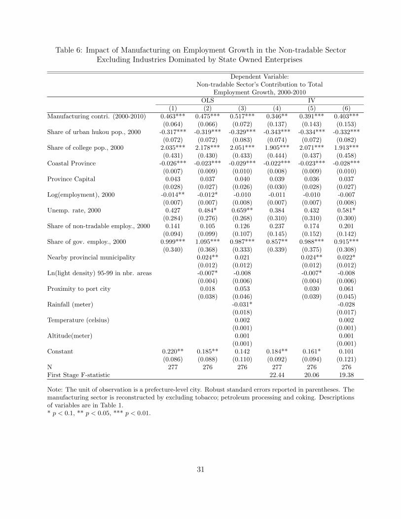
Table 6: Impact of Manufacturing on Employment Growth in the Non-tradable SectorExcluding Industries Dominated by State Owned Enterprises



(1) (2) (3) (4) (5) (6)Manufacturing contri. (2000-2010) 0.463*** 0.475*** 0.517*** 0.346** 0.391*** 0.403***



(0.431) (0.430) (0.433) (0.444) (0.437) (0.458)Coastal Province -0.026*** -0.023*** -0.029*** -0.022*** -0.023*** -0.028***


(0.028) (0.027) (0.026) (0.030) (0.028) (0.027)Log(employment), 2000 -0.014** -0.012* -0.010 -0.011 -0.010 -0.007

(0.007) (0.007) (0.008) (0.007) (0.007) (0.008)Unemp. rate, 2000 0.427 0.484* 0.659** 0.384 0.432 0.581*

(0.284) (0.276) (0.268) (0.310) (0.310) (0.300)Share of non-tradable employ., 2000 0.141 0.105 0.126 0.237 0.174 0.201

(0.094) (0.099) (0.107) (0.145) (0.152) (0.142)Share of gov. employ., 2000 0.999*** 1.095*** 0.987*** 0.857** 0.988*** 0.915***

(0.340) (0.368) (0.333) (0.339) (0.375) (0.308)Nearby provincial municipality 0.024** 0.021 0.024** 0.022*

(0.012) (0.012) (0.012) (0.012)Ln(light density) 95-99 in nbr. areas -0.007* -0.008 -0.007* -0.008

(0.004) (0.006) (0.004) (0.006)Proximity to port city 0.018 0.053 0.030 0.061

(0.038) (0.046) (0.039) (0.045)Rainfall (meter) -0.031* -0.028


(0.001) (0.001)Altitude(meter) 0.001 0.001

(0.001) (0.001)Constant 0.220** 0.185** 0.142 0.184** 0.161* 0.101


Note: The unit of observation is a prefecture-level city. Robust standard errors reported in parentheses. Themanufacturing sector is reconstructed by excluding tobacco; petroleum processing and coking. Descriptionsof variables are in Table 1.* p < 0.1, ** p < 0.05, *** p < 0.01.

31

Table 7: Impact of High- and Low-Technology Manufacturing on Employment Growth inthe Non-tradable Sector

Dependent Variable:Non-tradable Sector’s Contribution to Total Employment Growth, 2000-2010

OLS IV(1) (2) (3) (4) (5) (6)

High tech manu. contri. (2000-2010) 0.596*** 0.606*** 0.641*** 0.526** 0.572** 0.621**(0.137) (0.148) (0.158) (0.239) (0.244) (0.265)

Low tech manu. contri. (2000-2010) 0.438*** 0.466*** 0.492*** -0.016 -0.029 -0.061(0.078) (0.083) (0.088) (0.135) (0.157) (0.164)

Share of urban hukou pop., 2000 -0.318*** -0.335*** -0.345*** -0.372*** -0.379*** -0.359***(0.073) (0.076) (0.084) (0.087) (0.085) (0.093)

Share of college pop., 2000 2.015*** 2.182*** 2.041*** 1.373** 1.387** 1.174**(0.458) (0.452) (0.449) (0.541) (0.549) (0.572)

Coastal Province -0.026*** -0.022** -0.027** -0.018* -0.025** -0.026**(0.009) (0.010) (0.011) (0.010) (0.011) (0.013)

Province Capital 0.052* 0.042 0.044 0.057 0.056 0.057(0.031) (0.030) (0.028) (0.037) (0.035) (0.035)

Log(employment), 2000 -0.015** -0.011 -0.009 -0.009 -0.009 -0.005(0.007) (0.008) (0.008) (0.008) (0.008) (0.009)

Unemp. rate, 2000 0.411 0.525* 0.696** 0.344 0.358 0.494(0.302) (0.301) (0.298) (0.326) (0.328) (0.333)

Share of non-tradable employ., 2000 0.092 0.064 0.091 0.396** 0.403** 0.407**(0.105) (0.109) (0.111) (0.157) (0.170) (0.159)

Share of gov. employ., 2000 1.497** 1.709** 1.632** 0.376 0.478 0.825(0.742) (0.773) (0.760) (0.910) (1.004) (0.905)

Nearby provincial municipality 0.025* 0.021 0.027* 0.025*(0.013) (0.013) (0.014) (0.014)

Ln(light density) 95-99 in nbr. areas -0.009** -0.011* -0.009* -0.012*(0.005) (0.006) (0.005) (0.007)

Proximity to port city 0.015 0.042 0.063 0.068(0.038) (0.046) (0.046) (0.053)

Rainfall (meter) -0.031* -0.026(0.018) (0.018)

Temperature (celsius) 0.002 0.003**(0.001) (0.001)

Altitude(meter) 0.001 0.000(0.001) (0.001)

Constant 0.229** 0.173* 0.132 0.180* 0.137 0.063(0.093) (0.099) (0.122) (0.099) (0.104) (0.133)

N 260 259 259 260 259 259First Stage F-statistic 25.37 22.25 18.46

Note: The unit of observation is a prefecture-level city. Robust standard errors reported in parentheses. Thehigh- and low-technology manufacturing industries are classified based on NBS High-Technology Industry(Manufacturing Industry) Classifications (2013). Details of the classification are in Appendix Table C.9.Instruments are group specific. Corresponding first-stage estimates for columns (4) and (6) are reported inAppendix Table C.5. Descriptions of variables are in Table 1.* p < 0.1, ** p < 0.05, *** p < 0.01.

32

Table 8: Impact of High- and Low-Tech Manu. on Employment Growth in theNon-tradable Sector, Alternative Definition of High- and Low-Tech Manu. Industries


OLS IV(1) (2) (3) (4) (5) (6)

High tech manu.contri. 0.625*** 0.823(45% cutoff) (0.170) (0.609)Low tech manu. contri. 0.463*** 0.181(45% cutoff) (0.074) (0.182)High tech manu. contri. 0.652*** 0.575**(40% cutoff) (0.121) (0.270)Low tech manu. contri. 0.396*** -0.087(40% cutoff) (0.082) (0.136)High tech manu. contri. 0.558*** 0.395**(35% cutoff) (0.111) (0.197)Low tech manu. contri. 0.422*** -0.167(35% cutoff) (0.089) (0.190)N 260 260 260 260 260 260First Stage F-statistic 6.64 26.31 21.15

Note: The unit of observation is a prefecture-level city. Robust standard errors reported in parentheses. Allbaseline controls are included. The high- and low-technology manufacturing industries are classified basedon education level. Details of the classification are in Appendix Table C.9.* p < 0.1, ** p < 0.05, *** p < 0.01.

33

Table 9: Impact of Manufacturing on Employment Growth in Specific Non-TradableIndustries

Non-tradable Industry OLS IVUtility 0.003 0.007

(0.004) (0.010)

Construction 0.101*** -0.071(0.022) (0.063)

Transport, post and telecom services; 0.035** 0.046adminstration of water, (0.014) (0.030)environment, and public facilities

Whole sale,retail, catering 0.209*** 0.192***(0.024) (0.059)

Finance 0.009*** 0.022***(0.003) (0.007)

Real estate 0.019** 0.022***(0.004) ( 0.006)

Health care,sports and welfare 0.011*** 0.014***(0.002) (0.004)

Education, culture and entertainment 0.023*** 0.039***(0.004) (0.008)

Scientific research, polytechnic services, 0.010*** 0.018**and geological prospecting (0.002) (0.007)

Resident and other services 0.023*** 0.001(0.008) (0.014)

Others 0.045*** 0.068***(0.007) (0.015)

Note: The unit of observation is a prefecture-level city. Robust standard errors reported in parentheses.Each row is a separate regression and the dependent variable is the employment growth contributed by eachnon-tradable industry. Each regression includes the baseline controls.* p < 0.1, ** p < 0.05, *** p < 0.01.

34

Table 10: Impact of High(Low) Tech Manufacturing on Employment Growth in Low(High) Tech Manufacturing,

Dependent Variable:High (Low) Tech Manu’s Contribution to

Total Employment Growth, 2000-2010OLS IV

(1) (2) (3) (4)High-Tech Low Tech High-Tech Low-Tech

Low tech manu. contri. 0.141** 0.832**(0.071) (0.413)

High tech manu. contri. 0.400** 0.068(0.183) (0.279)

Share of urban hk pop.,2000 -0.091* -0.061 -0.020 -0.096(0.051) (0.052) (0.068) (0.062)

Share of college pop.,2000 0.429 -1.538*** 1.429 -1.463***(0.315) (0.384) (0.889) (0.347)

Region (coastal=1) 0.006* 0.014** -0.006 0.016**(0.004) (0.007) (0.008) (0.007)

Capital -0.050*** 0.037** -0.063** 0.021(0.018) (0.017) (0.027) (0.017)

Log(Employment),2000 0.009** 0.007 0.002 0.010(0.004) (0.006) (0.006) (0.006)

Unemp. rate,2000 -0.049 -0.111 0.046 -0.134(0.141) (0.136) (0.159) (0.148)

Share of non-tradable employ.,2000 0.220*** 0.500*** -0.211 0.602***(0.074) (0.099) (0.281) (0.129)

Share of gov. employ.,2000 -0.490 -2.015*** 1.129 -2.287***(0.337) (0.534) (0.883) (0.535)

Constant -0.121** -0.035 -0.060 -0.079(0.052) (0.075) (0.065) (0.079)

N 260 260 260 260First Stage F-statistic 5.72 21.23

Note: The unit of observation is a prefecture-level city. Robust standard errors reported in parentheses.Descriptions of variables are in Table 1. * p < 0.1, ** p < 0.05, *** p < 0.01.

35

Table 11: Impact of Manufacturing on Employment Growth in the Non-tradable SectorCoastal vs Inland Effects



(1) (2) (3) (4) (5) (6)Manufacturing contri. 0.557*** 0.551*** 0.667*** 0.842*** 0.913*** 0.886***

(0.087) (0.093) (0.109) (0.287) (0.310) (0.277)Manu. employ. contri. x Coastal -0.137 -0.110 -0.207* -0.500** -0.520** -0.489**Province (0.112) (0.117) (0.125) (0.232) (0.238) (0.200)Share of urban hukou pop., 2000 -0.308*** -0.312*** -0.311*** -0.278*** -0.280*** -0.288***


(0.458) (0.456) (0.468) (0.449) (0.448) (0.479)Coastal Province -0.020** -0.018* -0.022** -0.007 -0.000 -0.013


(0.028) (0.028) (0.026) (0.030) (0.029) (0.027)Log(employment), 2000 -0.013* -0.011 -0.008 -0.012 -0.012 -0.007

(0.007) (0.007) (0.008) (0.007) (0.008) (0.008)Unemp. rate , 2000 0.386 0.454 0.612** 0.303 0.420 0.580**


(0.097) (0.102) (0.106) (0.150) (0.160) (0.139)Share of gov. employ., 2000 0.979*** 1.068*** 0.894*** 0.971** 1.078** 0.783***

(0.338) (0.367) (0.308) (0.388) (0.442) (0.294)Nearby provincial municipality 0.023** 0.020* 0.023** 0.020*

(0.012) (0.012) (0.010) (0.012)Ln(light density) 95-99 in nbr. areas -0.006 -0.005 -0.002 -0.001

(0.004) (0.006) (0.004) (0.006)Proximity to port city 0.012 0.052 -0.024 0.049

(0.039) (0.045) (0.045) (0.043)Rainfall (meter) -0.031* -0.034*

(0.017) (0.017)Temperature 0.001 0.001

(0.001) (0.001)Altitude(meter) 0.001 0.002*

(0.001) (0.001)Constant 0.205** 0.181** 0.115 0.180* 0.190* 0.084


Note: The unit of observation is a prefecture-level city. Robust standard errors reported in parentheses.A prefecture-level city is assigned a region dummy taking a value of 1 if it is in the coastal provinces ofHebei, Liaoning, Jiangsu, Zhejiang, Fujian, Shandong, and Guangdong. Corresponding first-stage estimatesfor columns (4) and (6) are reported in Appendix Table C.8. Descriptions of variables are in Table 1.* p < 0.05, ** p < 0.01, *** p < 0.001.

36

A Harmonizing Regions and Industries

A.1 Harmonizing Administrative Regions across Censuses

Due to administrative reforms between 2000 and 2010, the prefecture-level cities reported in the censuses of2000 and 2010 are not identical. In order to have a larger sample, we use prefecture-level cities in 2010 asa benchmark, track each prefecture-level city to its corresponding areas in 2000, and study the employmentgrowth during this period. 26 Here we illustrate four main types of administrative changes and methodsemployed to adjust the unit of analysis. First, a city in the census of 2010 that was a county or a county-levelcity in the census of 2000. For example, Zhongwei city was a prefecture-level city in Ningxia province in 2010,but it was a county administrated under Wuzhong city in 2000. The census of 2000 reports the employmentdata for Wuzhong city, which includes Zhongwei county. The census of 2010 reports the employment forWuzhong and Zhongwei cities. We combine Wuzhong city and Zhongwei city in 2010 to compare to Wuzhongcity in 2000. Secondly, a city in 2010 was expanded from a prefecture-level city and its surrounding prefecturein 2000. For example, Nanning city in Guangxi province in 2010 consists of the Nanning city and part ofNanning diqu in 2000. The rest part of Nanning diqu in 2000 becomes Chongzuo city in 2010. We combineNanning city and Nanning diqu in 2000 to compare to the combination of Nanning City and ChongzuoCity in 2010. Thirdly, a city in the census of 2010 was a prefecture in 2000. For example, Baoshan cityin Yunnan province in 2010 was Baoshan prefecture in 2000. This type of change usually doesn’t occur inexpanding or declining areas, so they are comparable. Fourth, a city in the census of 2010 administeredmore or fewer counties. This change is mainly because some counties were administered by different upperprefecture-level cities in the two censuses. In fact, most types of changes between 2000 and 2010 are of thethird variety, which is not a concern to compare the data between the two censuses. We adjust the unitof analysis for the first two types. We exclude cities in Hainan province because the government restrictsmanufacturing industries to protect the local environment for tourism development. We also drop Tibet dueto data limitations. The final sample includes 277 prefecture-level cities.

A.2 Harmonizing Industrial Classification Systems

In China, GB/T4754 is the industries classification system. The first formal classification was issued in1984, called GB/T4754-1984 (Holz, 2013). The classification standards were later revised in 1994, 2000,and 2011, and the labels are GB/T47540-1994 (GB94), GB/T4754-2002 (GB02), and GB/T4754-2011(GB11) respectively. The 2000 Population Census used GB/T4754-1994, and the 2010 Population Censusused GB/T4754-2002. Following Holz (2013), and documentation of GB94 and GB02, we first constructcomparable 2-digit industries in manufacturing. Table A.1 illustrates the classification used in the paper.We reclassified the crafts and art production to other in the census of 2010 because this term was includedin the “other” category in the census of 2000.

Table A.1: Comparable 2-digit Manufacturing Industries

Census 2000 Census 2010

1 13. food processing 12. processing of food from agric. products14. food manufacturing 13. manufacture of foods

2 15.manufacture of beverages 14. manufacture of beverages3 16.manufacture of tobacco 15. manufacture of tobacco4 17.textile industry 16. manufacture of textiles

26Different administrative reforms at the prefecture level began in 1983, including converting a prefectureto a prefecture-level city, promoting a county-level city to a prefecture-level city, expanding the currentprefecture-level city by absorbing nearby counties or prefectures.

37

5 18. garments and other fiber products 17. manufacture of textiles, apparel, footwearand caps

6 19. leathers, furs, down and related products 18. manufacture of leather, fur, feather andrelated products

7 20. Timber processing, bamboo, canes, palm, fiber 19. Timber processing, bamboo, canes, palm,and straw products fiber and straw products

8 21.furniture manufacturing 20. furniture manufacturing9 22. papermaking and paper products 21. manufacture of paper and paper prod.10 23. printing industry 22. printing and recorded media11 24. cultural, education and sports good 23. cultural, education and sports good12 25. petroleum processing and coking 24. processing of petroleum, coking, nuclear fuel13 26. raw chemical materials and chemical products 25.manufacture of chemical raw materials and

chemical products14 27. medical and pharmaceutical products 26. manufacture of medicines15 28. chemical fiber 27. manufacture of chemical fiber16 29.rubber products 28. rubber products17 20. plastic products 29. plastic products18 31. nonmetal mineral products 30. nonmetal mineral products19 32. smelting and pressing of ferrous metals 31. smelting and pressing of ferrous metals20 33. smelting and pressing of nonferrous metals 32. smelting and pressing of nonferrous metals21 34. metal products 33. metal products22 35. ordinary machinery 34. manufacture of general purpose machinery

36. special purpose equipment 35. manufacture of special purpose machinery38. weapons and ammunition manufacturing

23 37. transport equipment 36. transport equipment24 39. electric equipment and machinery 37. electric equipment and machinery25 40. electronic and telecommunications equipment 38. manufacture of communication equipment,

computers and other26 41. instruments, meters, cultural and 39. manufacture of measuring instruments and

office equipment machinery for cultural activity and office work27 42. other manufacturing 40. manufacturing of artwork and

other manufacturing41. recycling and disposal of waste

Note: The No. listed in the first column indicate a category constructed by the author. The No. listedin the second and third columns are from population census 2000 and 2010 by each province, representingtwo-digit industry. The english titles are from Holz (2013).

38

Table A.2: Comparable 1-digit Non-tradable Sector

industry Census 2000 Census 20101 IV.utilities IV.utilities2 V. construction V. construction3 VII. transport, storage, post and VI.transport, storage, and postal services

telecommunication servicesVI50.water management XIV. adminstration of water, environment,

and public facilitiesXI71. Public Services

4 VIII. wholesale and retail trades, VIII. wholesale and retail tradesand catering services

IX. accommodation and cateringless IX63. accommodation

5 IX. finance and insurance X. finance6 X. real estate XI. real estate7 XII. health care, sports, and social welfare XVII. health care, social insurance/welfare

XVIII88. sports8 XIII. education, culture and arts, radio, film, XVI. education

and televisionXVIII. culture, sports and entertainmentless XVIII89.entertainmentless XVIII88.sports

9 XIV. scientific research and polytechnic services XIII. scientific research, polytechnic services,VI46.geological prospecting and geological prospecting

10 XI72. residence Services XV. resident and other services11 XI.social service VII. information transfer, computer services,

less XI71. public services and softwareless XI72. residence services XII. leasing and commercial services

IX63. accommodationXVIII89.entertainment

Note: The No. listed in the first column indicate a category constructed by the author. The roman numberlisted in the second and third columns are from population census 2000 and 2010, which represents 1-digitindustry. The numeric number listed in the second and third columns represents 2-digit industry. Theenglish titles are from Holz (2013).

39

B Data sources

Table B.1: Variables, Descriptions, and Sources

Variable Description and Sources

Variables in regression:

Non-tradable sec. contri. tototal employ. growth (%)

Change in non-tradable employment 2000-2010 normalized by total 2000 localemployment. Source : Tabulation on the Population Census of the People’s Republic ofChina by County (2000, 2010).

Manu. contri. to total employ.growth (%)

Change in manufacturing employment 2000-2010 normalized by total 2000 localemployment. Source : Tabulation on the Population Census of the People’s Republic ofChina by County (2000, 2010).

Manu. contri. to total employ.growth (%)

Change in manufacturing employment 2010-2013 normalized by total 2000 localemployment. Source : China City Statistical Yearbook (2011, 2014).

High (low) tech manu. contri.to total employ. growth (%)

Change in high (low) manufacturing employment 2000-2010 normalized by total 2000local employment. Source: Tabulation on the Population Census, published by province(2000, 2010).

Share of urban hukoupop.(%), 2000

Population with urban hukou divided by local population. Source : Tabulation on thePopulation Census of the People’s Republic of China by County (2000).

Share of college pop. (%),2000

Population with college education and above divided by age 6+ population. Source:Tabulation on the Population Census of the People’s Republic of China by County(2000).

Coastal Province A dummy variable equals one if the prefecture-level city is in the coastal provinces ofHebei, Liaoning, Jiangsu, Zhejiang, Fujian, Shandong, and Guangdong.

Province Capital A dummy variable which equals one if the prefecture-level city is the capital of theprovince.

Log employment,2000 Log value of local employment in 2000. Source : Tabulation on the Population Censusof the People’s Republic of China by County (2000).

Unemployment rate(%), 2000 Unemployment rate in 2000. Source : Tabulation on the Population Census, publishedby province (2000).

Share of non-tradable employ.(%), 2000

Non-tradable employment divided by local employment. Source : Tabulation on thePopulation Census of the People’s Republic of China by County (2000).

Share of gov. employ. (%),2000

Government employment divided by local employment. Source : Tabulation on thePopulation Census of the People’s Republic of China by County (2000).

Nearby provincialmunicipality

A dummy variable that equals to 1 if the prefecture-level city has a common border withone of provincial municipalities including Beijing, Shanghai, Tianjin, and Chongqing.

Log night light density1995-1999 in nbr. areas

Log value of average light density in neighboring areas from 1995-1999. Neighboringcities are identified in ArcGIS. Source: National Geographical Data Center;Center forInternational Earth Science Information Network.

Proximity to nearest port city Reciprocal of one plus distance to the nearest port city in thousands of kilometers.Distance to the nearest port city are calculated in ArcGIS.

Rainfall (meters) Average precipitation from 1950-2000. Source: Global Climate Data.Temperature (Celsius) Average temperature from 1950-2000. Source: Global Climate Data.Altitude (100 meters) Average altitude in each city. Source: Global Climate Data.

Variables not in regressionEmployment Share by Sector Source: China Population and Employment Statistics Yearbook (2011).China’s Share WorldManufacturing Output

Manufacturing output in China divided by World manufacturing output. Source:World Bank World Development Indicators.

Manufacturing Growth inChina

Annual growth of firms and employment from 2000-2010. Source: Industrial EconomyStatistical Yearbook (2001-2011).

SOE output by industry SOE output divided by total output by industry (2000, 2010). Source:China RegionalStatistical Yearbook (2001, 2011).

Education by industry Source: National Population Census (2010).

40

C Appendix Tables

Table C.1: First Stage Regressions For Table 3,Impact of Manufacturing on Employment Growth in the Non-tradable Sector

Dependent Variable:Manufacturing’s Contribution to

Total Employment Growth, 2000-2010(0) (1) (2) (3)

instrument in baseline model 0.937*** 1.118*** 0.916*** 0.891***(0.112) (0.169) (0.188) (0.191)

Share of urban hk pop.,2000 -0.133 -0.187** -0.176**(0.082) (0.083) (0.081)

Share of college pop.,2000 -0.640 -1.051** -1.072**(0.539) (0.492) (0.483)

Region (coastal=1) 0.012 0.007 0.008(0.009) (0.008) (0.008)

Capital 0.008 -0.003 -0.001(0.025) (0.025) (0.024)

Log(employment),2000 0.001 0.012* 0.011(0.006) (0.007) (0.007)

Unemp. rate,2000 -0.109 -0.218 -0.211(0.215) (0.189) (0.190)

Share of non-tradable employ.,2000 0.325*** 0.345***(0.105) (0.110)

Share of gov. employ.,2000 -0.448(0.506)

Constant -0.004 0.035 -0.116 -0.098(0.006) (0.078) (0.083) (0.086)

N 277 277 277 277Rsquare 0.37 0.55 0.57 0.58First stage statistics 43.77 23.88 21.84

Note: The unit of observation is a prefecture-level city. Robust standard errors reported in parentheses. Theinstrumental variable is equal to the 2000 share of manufacturing employment for a given city multipliedby the 2000-2010 growth rate in national manufacturing employment (exclude own city). Descriptions ofvariables are in Table 1.* p < 0.1, ** p < 0.05, *** p < 0.01.

41

Table C.2: First Stage Regressions for Table 4Robustness to Spatial and Geographical Characteristics

Dependent Variable:Manufacturing’s Contribution to

Total Employment Growth, 2000-2010(1) (2)

Instrument 0.851*** 0.831***(0.192) (0.191)

Share of urban hukou pop.,2000 -0.151* -0.095(0.078) (0.081)

Share of college pop.,2000 -1.122** -1.065**(0.472) (0.447)

Coastal Province -0.009 0.003(0.010) (0.009)

Province Capital 0.004 0.001(0.023) (0.024)

Log(employment),2000 0.008 0.007(0.007) (0.007)

Unemp. rate,2000 -0.369** -0.346*(0.187) (0.203)

Share of non-tradable employ.,2000 0.357*** 0.284***(0.113) (0.105)

Share of gov. employ.,2000 -0.444 0.090(0.538) (0.267)

Nearby provincial municipality 0.012 0.014(0.017) (0.017)

Ln(light density) 1995-99 in nbr. areas -0.005 -0.010**(0.004) (0.004)

Proximity to port city 0.106*** 0.028(0.034) (0.033)

Rainfall (meter) 0.004(0.013)

Temperature (celsius) 0.003***(0.001)

Altitude(meter) -0.002***(0.001)

Constant -0.134 -0.113(0.089) (0.098)

N 276 276First Stage F-statistic 19.60 18.99

Note: The unit of observation is a prefecture-level city. Robust standard errors reported in parentheses. Theinstrumental variable is equal to the 2000 share of manufacturing employment for a given city multipliedby the 2000-2010 growth rate in national manufacturing employment (exclude own city). Descriptions ofvariables are in Table 1.* p < 0.1, ** p < 0.05, *** p < 0.01.

42

Table C.3: Impact of Manufacturing on Employment Growth in the Non-tradable Sector,Province Fixed Effects Estimates



(1) (2) (3) (4) (5) (6)Manufacturing contri. (2000-2010) 0.480*** 0.487*** 0.476*** 0.363*** 0.366** 0.361**




(0.031) (0.033) (0.031) (0.027) (0.027) (0.027)Log(employment), 2000 -0.017** -0.018** -0.017** -0.014* -0.016** -0.015**

(0.007) (0.007) (0.007) (0.008) (0.008) (0.007)Unemp. rate, 2000 0.946*** 0.954*** 0.984*** 0.922*** 0.925*** 0.974***


(0.093) (0.110) (0.113) (0.122) (0.133) (0.137)Share of gov. employ., 2000 1.051** 0.972** 0.991** 1.008*** 0.949*** 0.980***

(0.418) (0.382) (0.412) (0.363) (0.342) (0.363)Nearby provincial municipality 0.013* 0.016* 0.016 0.019

(0.007) (0.008) (0.015) (0.015)Ln(light density)95-99 in nbr. areas -0.008 -0.008 -0.005 -0.007

(0.006) (0.007) (0.007) (0.007)Proximity to port city 0.088 0.101 0.100* 0.114**

(0.070) (0.063) (0.058) (0.055)Rainfall (meter) -0.003 -0.007


(0.006) (0.004)Altitude(meter) 0.002 0.002

(0.004) (0.003)Constant 0.253*** 0.212** 0.130

(0.087) (0.091) (0.136)N 277 276 276 276 275 275First Stage F-statistic 14.67 11.15 13.46

Note: The unit of observation is a prefecture-level city. Robust standard errors reported in parentheses. Allestimates include province fixed effects. Descriptions of variables are in Table 1. * p < 0.1, ** p < 0.05, ***p < 0.01.

43

Table C.4: Impact of Manufacturing on Employment Growth in the Non-tradable SectorRobustness to Contemporaneous Variables

Panel A: OLS EstimatesDependent Variable:

Non-tradable Sector’s Contribution toTotal Employment Growth, 2000-2010

(1) (2) (3) (4)Manufacuturing contri. (2000-2010) 0.458*** 0.460*** 0.472*** 0.515***

(0.065) (0.061) (0.066) (0.066)Growth of Fixed Asset Investment (2000-2010) 0.165***

(0.056)Growth of FDI (2000-2010) 0.011

(0.026)Growth of Gov. Expenditure (2000-2010) 0.166**

(0.072)Growth of Wages (2000-2010) 0.539***

(0.174)N 256 243 256 255Rsquare 0.60 0.61 0.60 0.60

Panel B: IV EstimatesDependent Variable:

Non-tradable Sector’s Contribution toTotal Employment Growth, 2000-2010

(1) (2) (3) (4)Manufacuturing contri. (2000-2010) 0.350*** 0.262** 0.397*** 0.382***

(0.133) (0.119) (0.126) (0.144)Growth of Fixed Asset Investment (2000-2010) 0.180***

(0.056)Growth of FDI (2000-2010) 0.005

(0.026)Growth of Gov. Expenditure (2000-2010) 0.169**

(0.070)Growth of Wages (2000-2010) 0.443**

(0.206)N 256 243 256 255First stage statistics 22.58 19.34 24.14 20.83

Note: Each regression includes following control variables from baseline regression: Share of urbanhk pop.,2000; Share of college pop.,2000; Region (coastal=1), Capital, Log(employment),2000; Unemp.rate,2000; Share of non-tradable employ.,2000; and Share of gov. employ.,2000.* p < 0.1, ** p < 0.05, *** p < 0.01.

44

Table C.5: First Stage Regressions for Table 7High- and Low-technology Manufacturing Industries Analysis

Model 1 Model 2High skill Low skill High skill Low skill

manu. contri. manu. contri. manu. contri. manu. contri.Instrument (high-tech. manu.) 0.718*** -1.048*** 0.663*** -1.013***

(0.169) (0.239) (0.160) (0.227)Instrument (low-tech. manu.) 0.025 0.912*** 0.048 0.827***

(0.097) (0.124) (0.081) (0.118)Share of urban hukou pop., 2000 -0.065 -0.078 -0.022 -0.028

(0.041) (0.055) (0.041) (0.059)Share of college pop., 2000 -0.201 -0.644* -0.139 -0.699**

(0.219) (0.347) (0.181) (0.321)Coastal Province 0.002 0.006 -0.007 0.001

(0.003) (0.007) (0.004) (0.008)Province Capital -0.022* 0.007 -0.019* 0.008

(0.011) (0.016) (0.010) (0.016)Log(employment), 2000 0.006* 0.007 0.004 0.005

(0.003) (0.005) (0.003) (0.006)Unemp. rate, 2000 -0.069 -0.171 -0.105 -0.374**

(0.114) (0.142) (0.106) (0.168)Share of non-tradable employ.,2000 0.187*** 0.256*** 0.120** 0.232***

(0.068) (0.092) (0.048) (0.076)Share of gov. employ., 2000 -0.292 -1.055** -0.200 -0.253

(0.279) (0.467) (0.293) (0.532)Nearby provincial municipality 0.012 0.003

(0.011) (0.008)Ln(light density) 1995-99 in nbr. areas 0.002 -0.006

(0.002) (0.004)Proximity to port city 0.022 0.026

(0.014) (0.029)Rainfall (meter) 0.001 0.011

(0.005) (0.010)Temperature (celsius) 0.001 0.002*

(0.000) (0.001)Altitude(meter) -0.000 -0.001**

(0.000) (0.001)Constant -0.070 -0.047 -0.075 -0.075

(0.046) (0.069) (0.050) (0.083)N 260 260 259 259First Stage F-statistic 25.37 18.46Note: The unit of observation is a prefecture-level city. Robust standard errors reported in parentheses.Descriptions of variables are in Table 1.* p < 0.1, ** p < 0.05, *** p < 0.01.

45

Table C.6: Impact of High- and Low-Technology Manufacturing on Employment GrowthRobustness to Share of Pop. in High School

Dependent Variable:Non-tradable Sector’s Contribution to Total Employment Growth, 2000-2010

OLS IV(1) (2) (3) (4) (5) (6)

High tech manu. contri. 0.663*** 0.668*** 0.707*** 0.675*** 0.703*** 0.785***(0.147) (0.160) (0.173) (0.211) (0.223) (0.244)

Low tech manu. contri. 0.440*** 0.461*** 0.486*** 0.018 0.000 -0.026(0.075) (0.082) (0.087) (0.132) (0.154) (0.161)

Share of urban hk pop.,2000 -0.252*** -0.278*** -0.285*** -0.302*** -0.318*** -0.298***(0.078) (0.079) (0.085) (0.086) (0.084) (0.089)

Share of college pop.,2000 2.432*** 2.495*** 2.364*** 1.759*** 1.721*** 1.533**(0.506) (0.499) (0.490) (0.572) (0.584) (0.610)

Share of high school pop.,2000 -0.451** -0.369** -0.390** -0.388** -0.346* -0.387**(0.181) (0.178) (0.181) (0.186) (0.186) (0.194)

Coastal Province -0.026*** -0.022** -0.027** -0.019* -0.024** -0.025**(0.009) (0.010) (0.011) (0.010) (0.011) (0.012)

Province Capital 0.041 0.034 0.036 0.051 0.050 0.052(0.032) (0.031) (0.030) (0.036) (0.035) (0.034)

Log(employment),2000 -0.014* -0.010 -0.008 -0.010 -0.008 -0.005(0.007) (0.008) (0.009) (0.008) (0.008) (0.009)

Unemp. rate,2000 0.264 0.383 0.554* 0.227 0.247 0.388(0.321) (0.315) (0.311) (0.330) (0.332) (0.335)

Share of non-tradable employ.,2000 0.094 0.069 0.097 0.349** 0.365** 0.371**(0.106) (0.111) (0.113) (0.149) (0.163) (0.150)

Share of gov. employ.,2000 1.793** 1.953** 1.895** 0.783 0.866 1.222(0.737) (0.780) (0.770) (0.893) (0.998) (0.919)

Nearby provincial municipality 0.019 0.015 0.021 0.018(0.013) (0.013) (0.013) (0.013)

Ln(light density) 1995-99 in nbr. areas -0.009** -0.011* -0.009* -0.013*(0.005) (0.006) (0.005) (0.007)

Proximate to port city 0.017 0.045 0.059 0.065(0.037) (0.045) (0.045) (0.051)

Rainfall (meter) -0.032* -0.030(0.018) (0.018)

Temperature (celsius) 0.002 0.003**(0.001) (0.001)

Altitude(meter) 0.001 0.000(0.001) (0.001)

N 260 259 259 260 259 259First Stage Statistics 21.11 19.88 15.37

Note: The unit of observation is a prefecture-level city. Robust standard errors reported in parentheses. Thehigh- and low-technology manufacturing industries are classified based on NBS High-Technology Industry(Manufacturing Industry) Classifications (2013). Details of the classification are in Appendix Table C.9.Instruments are group specific.* p < 0.1, ** p < 0.05, *** p < 0.01.

46

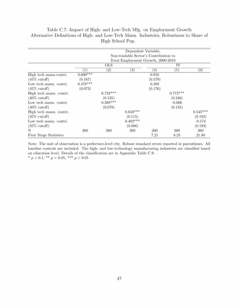
Table C.7: Impact of High- and Low-Tech Mfg. on Employment GrowthAlternative Definitions of High- and Low-Tech Manu. Industries, Robustness to Share of

High School Pop.


OLS IV(1) (2) (3) (4) (5) (6)

High tech manu.contri. 0.690*** 0.916(45% cutoff) (0.167) (0.579)Low tech manu. contri. 0.476*** 0.288(45% cutoff) (0.073) (0.176)High tech manu. contri. 0.733*** 0.772***(40% cutoff) (0.135) (0.246)Low tech manu. contri. 0.389*** -0.066(40% cutoff) (0.078) (0.135)High tech manu. contri. 0.633*** 0.545***(35% cutoff) (0.115) (0.182)Low tech manu. contri. 0.402*** -0.174(35% cutoff) (0.086) (0.193)N 260 260 260 260 260 260First Stage Statistics 7.21 8.25 21.88

Note: The unit of observation is a prefecture-level city. Robust standard errors reported in parentheses. Allbaseline controls are included. The high- and low-technology manufacturing industries are classified basedon education level. Details of the classification are in Appendix Table C.9.* p < 0.1, ** p < 0.05, *** p < 0.01.

47

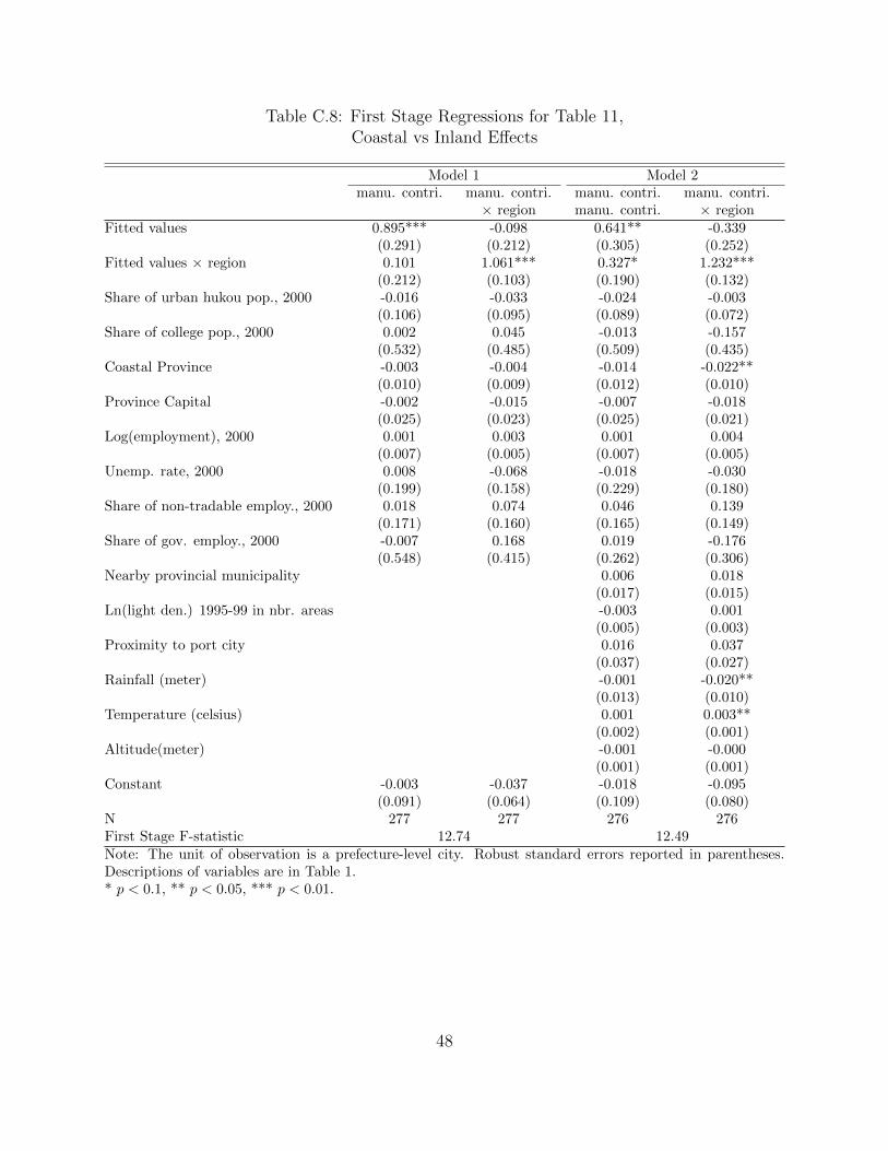
Table C.8: First Stage Regressions for Table 11,Coastal vs Inland Effects

Model 1 Model 2manu. contri. manu. contri. manu. contri. manu. contri.

× region manu. contri. × regionFitted values 0.895*** -0.098 0.641** -0.339

(0.291) (0.212) (0.305) (0.252)Fitted values × region 0.101 1.061*** 0.327* 1.232***

(0.212) (0.103) (0.190) (0.132)Share of urban hukou pop., 2000 -0.016 -0.033 -0.024 -0.003

(0.106) (0.095) (0.089) (0.072)Share of college pop., 2000 0.002 0.045 -0.013 -0.157

(0.532) (0.485) (0.509) (0.435)Coastal Province -0.003 -0.004 -0.014 -0.022**

(0.010) (0.009) (0.012) (0.010)Province Capital -0.002 -0.015 -0.007 -0.018

(0.025) (0.023) (0.025) (0.021)Log(employment), 2000 0.001 0.003 0.001 0.004

(0.007) (0.005) (0.007) (0.005)Unemp. rate, 2000 0.008 -0.068 -0.018 -0.030

(0.199) (0.158) (0.229) (0.180)Share of non-tradable employ., 2000 0.018 0.074 0.046 0.139

(0.171) (0.160) (0.165) (0.149)Share of gov. employ., 2000 -0.007 0.168 0.019 -0.176

(0.548) (0.415) (0.262) (0.306)Nearby provincial municipality 0.006 0.018

(0.017) (0.015)Ln(light den.) 1995-99 in nbr. areas -0.003 0.001

(0.005) (0.003)Proximity to port city 0.016 0.037

(0.037) (0.027)Rainfall (meter) -0.001 -0.020**

(0.013) (0.010)Temperature (celsius) 0.001 0.003**

(0.002) (0.001)Altitude(meter) -0.001 -0.000

(0.001) (0.001)Constant -0.003 -0.037 -0.018 -0.095

(0.091) (0.064) (0.109) (0.080)N 277 277 276 276First Stage F-statistic 12.74 12.49Note: The unit of observation is a prefecture-level city. Robust standard errors reported in parentheses.Descriptions of variables are in Table 1.* p < 0.1, ** p < 0.05, *** p < 0.01.

48

Table C.9: Classification of High- and Low- Technology Manufacturing Industries

Cat. Industries % Employ. % Employ. High-Technology Manu.above above NBS above high schoolhigh school college 45% 40% 35%

14 26. manufacture of medicines 64 33.5 H H H H12 24. processing of petroleum, coking 63 30.4 L H H H

nuclear fuel3 15. manufacture of tobacco 61.2 29.9 L H H H22 34. general purpose machinery 36.4 12.5 H H H H

35. special purpose machinery 46.6 18.7 H H H H13 25.manufacture of chemical raw 45.9 18.4 L H H H

materials and chemical products23 36. transport equipment 45.6 18.3 H H H H25 38. manufacture of communication 44.6 16.2 H H H

equipment, computers and other19 31. smelting and pressing of 44.2 16.7 L L H H

ferrous metals20 32. smelting and pressing of 42.3 15.7 L L H H

nonferrous metals26 39. manufacture of measuring 41.5 17.0 H L H H

instruments and machinery forcultural activity and office work

2 14. manufacture of beverages 40.5 14.7 L L H H10 22. printing and recorded media 39.5 12.3 L L L H24 37. electric equipment and machinery 39.2 14.5 L L L H15 27. manufacture of chemical fiber 38.9 12.6 L L L H16 28. rubber products 30.8 9.2 L L L L21 33. metal products 26.1 7.1 L L L L9 21. manufacture of paper and 29.1 8.0 L L L L

paper prod.1 12. processing of food from 22.5 6.0 L L L L

agri. products13. manufacture of foods 29.4 9.7 L L L L

17 29. plastic products 24.2 6.2 L L L L18 30. nonmetal mineral products 23.1 6.1 L L L L11 23. cultural, education and sports 21.1 6.1 L L L L4 16. manufacture of textiles 19.8 4.0 L L L L8 20. furniture manufacturing 17.6 4.0 L L L L5 17. manufacture of textiles 15.6 3.1 L L L L

17. apparel, footwear and caps6 18. manufacture of leather 14.6 2.6 L L L L

18. fur, feather, etc.7 19. Timber processing, bamboo, 14.2 2.6 L L L L

canes, palm, fiber and straw products27 40. manufacture of artwork 18.5 4.7 L L L L

and other manufacturing41. recycling and disposal of waste 12.6 2.6 L L L L

Note: NBS classification is based on High-Technology Industry Classifications (2013). Education data arefrom National Population Census 2010. H (L) denotes high (low)-technology manufacturing industry.

49

manufacturing growth and local multipliers in china

Documents