map design: an on-the-road evaluation of the time to read ...driving/publications/umtri-98-4.pdf ·...
TRANSCRIPT
Technical Report UMTRI-98-4 June, 1998
Map Design: An On-the-Road Evaluation ofthe Time to Read Electronic Navigation Displays
Christopher Nowakowski and Paul Green
umtriHUMAN FACTORS
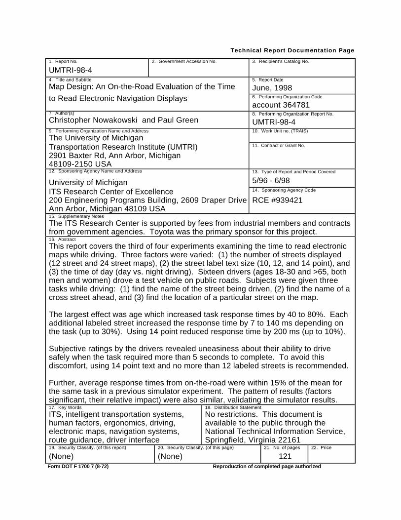
Technical Report Documentation Page
1. Report No.
UMTRI-98-42. Government Accession No. 3. Recipient’s Catalog No.
4. Title and Subtitle
Map Design: An On-the-Road Evaluation of the Time5. Report Date
June, 1998to Read Electronic Navigation Displays 6. Performing Organization Code
account 3647817. Author(s)
Christopher Nowakowski and Paul Green8. Performing Organization Report No.
UMTRI-98-49. Performing Organization Name and Address
The University of Michigan10. Work Unit no. (TRAIS)
Transportation Research Institute (UMTRI)2901 Baxter Rd, Ann Arbor, Michigan48109-2150 USA
11. Contract or Grant No.
12. Sponsoring Agency Name and Address
University of Michigan
13. Type of Report and Period Covered
5/96 - 6/98ITS Research Center of Excellence200 Engineering Programs Building, 2609 Draper DriveAnn Arbor, Michigan 48109 USA
14. Sponsoring Agency Code
RCE #939421
15. Supplementary Notes
The ITS Research Center is supported by fees from industrial members and contractsfrom government agencies. Toyota was the primary sponsor for this project.16. Abstract
This report covers the third of four experiments examining the time to read electronicmaps while driving. Three factors were varied: (1) the number of streets displayed(12 street and 24 street maps), (2) the street label text size (10, 12, and 14 point), and(3) the time of day (day vs. night driving). Sixteen drivers (ages 18-30 and >65, bothmen and women) drove a test vehicle on public roads. Subjects were given threetasks while driving: (1) find the name of the street being driven, (2) find the name of across street ahead, and (3) find the location of a particular street on the map.
The largest effect was age which increased task response times by 40 to 80%. Eachadditional labeled street increased the response time by 7 to 140 ms depending onthe task (up to 30%). Using 14 point reduced response time by 200 ms (up to 10%).
Subjective ratings by the drivers revealed uneasiness about their ability to drivesafely when the task required more than 5 seconds to complete. To avoid thisdiscomfort, using 14 point text and no more than 12 labeled streets is recommended.
Further, average response times from on-the-road were within 15% of the mean forthe same task in a previous simulator experiment. The pattern of results (factorssignificant, their relative impact) were also similar, validating the simulator results.17. Key Words
ITS, intelligent transportation systems,human factors, ergonomics, driving,electronic maps, navigation systems,route guidance, driver interface
18. Distribution Statement
No restrictions. This document isavailable to the public through theNational Technical Information Service,Springfield, Virginia 22161
19. Security Classify. (of this report)
(None)20. Security Classify. (of this page)
(None)21. No. of pages
12122. Price
Form DOT F 1700 7 (8-72) Reproduction of completed page authorized

ii
iii
UMTRI Technical Report 98-4
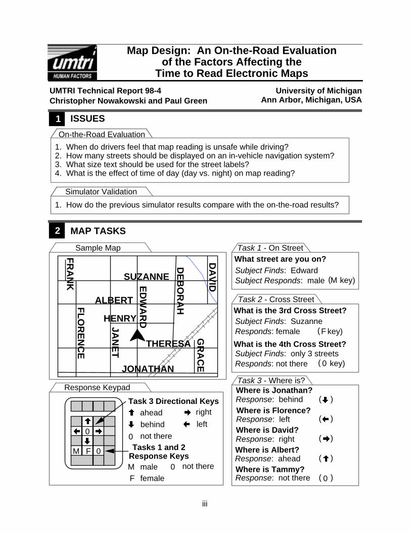
ISSUES1
MAP TASKS2
University of Michigan
Map Design: An On-the-Road Evaluationof the Factors Affecting the
Time to Read Electronic Maps
Christopher Nowakowski and Paul Green Ann Arbor, Michigan, USA
1. When do drivers feel that map reading is unsafe while driving?2. How many streets should be displayed on an in-vehicle navigation system?3. What size text should be used for the street labels?4. What is the effect of time of day (day vs. night) on map reading?
On-the-Road Evaluation
1. How do the previous simulator results compare with the on-the-road results?
Simulator Validation
GR
AC
E
JONATHAN
FR
AN
K SUZANNE
DE
BO
RA
HFL
OR
EN
CE
HENRY
ED
WA
RD
THERESA
ALBERTJA
NE
T
DA
VID
Sample Map
Response Keypad
Tasks 1 and 2Response Keys
malefemale
M F 0
0
Task 3 Directional Keys
left
right
behind
ahead
0 not there
Task 1 - On StreetWhat street are you on?Subject Finds: EdwardSubject Responds: male M( key)
What is the 3rd Cross Street?Subject Finds: SuzanneResponds: female
What is the 4th Cross Street?Subject Finds: only 3 streetsResponds: not there
Task 2 - Cross Street
( key)F
( key)0
Task 3 - Where is?
( )Where is Jonathan?Response: behindWhere is Florence?Response: leftWhere is David?Response: rightWhere is Albert?Response: aheadWhere is Tammy?Response: not there
( )
( )
( )
( )
0MF
0 not there
iv
METHOD3
ON-THE-ROAD EVALUATION RESULTS4
Main Test Conditons
10 POINT
12 POINT
14 POINT
Text Size 12 Streets 24 Streets
√ √√ √√ √
Age 18 - 30 Age >65
Men Women
2 2
2 2
1 2
Day Night
DayNight
Men Women
2 2
2 2
Subjects
Task 2 - Cross StreetTask 1 - On Street
Task 3 - Where is? Error Rates
Issue 1 - When is map reading unsafe?
1. Age Effect
0
5
10
15
20
1 2 3
24Streets
12 Streets
Err
or R
ate
(%)
Task
2. Number of Streets Effect
05
10152025
Err
or R
ate
(%)
1 2 3Task
Mature
Young
05
10152025
0 3 6Response Time (s)
21 4 5 7 8020406080100
Fre
quen
cy (
%)
Cum
ulat
ive
(%)
x = 1.8 sF
requ
ency
(%
)
Cum
ulat
ive
(%)
0
5
10
15
20
0 10025
50
75
100
Response Time (s)155
x = 3.4 s
0
5
10
15
0 10 200
25
50
75
100
155Response Time (s)
Fre
quen
cy (
%)
Cum
ulat
ive
(%)
x = 5.2 s
Very Safe
Very Unsafe
0 2 4 6 8Response Time (s)
31 75 9
54
3
21
Sometimes Unsafe
Safe
Unsafe
Session
Expressway Driving Scenario
ResponseKeypad
Map
Response Time Regression Equations (ms)
Issue 2 - How many streets to display?
Recommendation:
Display ≤12 Streets
Issue 3 - What text size to use?
(s)
1.51.61.71.81.92.0
10 12 14Point Size
24 st.
12 st.
Task 1 Point Size Effect Task 2 Point Size Effect
Recommendations:
1. When possible, Use 14 point.
2. Do not use <12 point
Issue 4 - Day/Night Effects
1.61.71.81.92.02.1
(s)
Session1 2
Task 1 - Night learning is more difficult
2
4
6
8
10
12 24Streets displayed
Mature
Young
(s)
Task 3 Streets Effect
0
50
100
150
(ms)
1 2 3Task
Response time increaseper each displayed street
Session
4.0
4.5
5.0
5.5
6.0
(s)
1 2NightDay
Task 3 - Night increases response time
Recommendation:
Issues of color,luminance, and contrastfor night-use mapsneed to be addressedin further reasearch.
Task 2 - Cross Street
+ 8.08*(P-12)*(SL)+ 40.83*(S-12)*[MINIMUM(1,X-2)]
Task 1 - On Street
Task 3 - Where is?
2.5
3.0
3.5
4.0
4.5
(s)
10 12 14Point Size
24 st.
12 st.
v
RT = 6710 + 325*(A) + 6.67*(S) + 33.75*(P)2 - 832.50*(P)
+ 9.58*(C)
RT = 1210 + 575*(A) + 370*(X) + 40.83*(S)
RT = [1630 + 1235*(A) + 380*(T) + 136*(S) + 27*(A)*(SL)
+ 475*(L)]*(SR)
vi
5 5
SIMULATOR VALIDATION RESULTS5
Age 18 - 30 Age 65<
Men
4 45 5
Women Men Women
4 4
Subjects
Simulator
Experiment
On-the-Road
Response Time Comparison
Differences in Experimental Findings
1000
1500
2000
2500
(ms)
10 12 14Point Size
On-the-Road
Simulator
Point Size
4000
5000
6000
7000
(ms)
10 12 14
Simulator
On-the-Road
Task 1 - Point Size Effects Task 3 - Point Size EffectsConclusions:The optimal point size was also dependent upon the display resolution and location (character visual angle).
Regression Equations Terms
A = Age -1 if young+1 if mature{
S = Number of streets (S ≥ 1)
P = Point size (10 ≤ P ≤14)X = Target cross street (X ≥ 1)
T = Time of day -1 for day+1 for night{
C = Clutter0 if ≤ 12 point(P-12)(S-12.52) if > 12 pt.{
SL = Street level-1*(24-S) if S ≤ 12+1*(S-12) if S > 12
{
L = Target location -1 if ahead 0 if not there+1 if behind, left or right
{
SR = Search result 1 if found1.70 if not found{
0255075
100
05
101520
05
1015
0 1 2 3 4 5Response Time (s)
Simulator
On-the-Road
Fre
quen
cy (
%)
Cum
ulat
ive
(%)
0255075
Task 1 - On Street
x = 1.64 s
x = 1.79 s
246
0255075
100
0246
Fre
quen
cy (
%)
0 5 10 15 20Response Time (s)
0255075
Cum
ulat
ive
(%)Simulator
On-the-Road
Task 3 - Where is?
x = 5.96 s
x = 5.20 s
Task 1 Task 3
6
24
24
48
Trials per Subject

vii
PREFACE
This research was funded by the University of Michigan Intelligent TransportationSystems (ITS) Research Center for Excellence, formerly the IVHS Research Center forExcellence. The program is a consortium of companies and government agencies,working with the University, whose goal is to advance ITS research andimplementation.
The current sponsors are:
• Ann Arbor Transit Authority• Automobile Association of America (AAA)• Chrysler Corporation• Federal Highway Administration (FHWA)• Ford Motor Company• General Motors Corporation• Hewlett Packard• Michigan Department of Transportation• Nissan Motors• NOVA Laboratories• Orbital Sciences• Road Commission of Oakland County• Ryder Trucks• Siemens Automotive• Toyota Motor Corporation
We would like to thank the lead corporate sponsor for this project, Toyota MotorCorporation, for their support. Originally Cale Hodder, and now Jim Bauer (both fromToyota), have served as project technical monitors.
Electronic maps are commonplace in automotive navigation systems in Japan, andsoon will be common in the U.S. and Europe. To make such maps safe and easy touse while driving, it is important to know how engineering, individual, and task factorsaffect reading time, and how reading time can be minimized. The more time driversspend looking in the vehicle, the less time they spend looking at the road, increasingthe opportunity for crashes. Given the almost complete absence of literature on thetime to read maps prior to this project, two specific issues were addressed.
Issue 1: How long does it take to read an electronic local map as a function of labelsize and orientation, the number of streets shown, the percentage of streetslabeled, display location, and the driver's task?
Issue 2: When do drivers desire area maps instead of turn (intersection) displays?
These issues were examined in 5 reports summarized on the next page:
viii
Green, P. (1998). Reading Electronic Area Maps: An Annotated Bibliography ,(Technical Report UMTRI-98-38).
This report contains a collection of abstracts generated by the author.Primary articles concerned performance differences in reading streetnames due to font, how people follow directions using street maps, etc.There were no articles in the literature that methodically considered howfactors related to street map design affect task completion time.Secondary articles considered color coding, symbols for touristinformation, etc.
Authors to be determined (1998). Preliminary Examinations of the Time to ReadElectronic Maps: The Effects of Text and Graphic Characteristics , (Technical ReportUMTRI-98-36).
This report summarizes the initial series of simulator experimentsconcerning reading electronic maps. Included were efforts to identifyrepresentative maps and street names for testing and a pilot experimentconcerning the subjective legibility of various map typefaces. In the mainexperiment, the time to read the electronic maps was found as a functionof text size, the number of streets, text orientation, and grid-likeness.
Brooks, A. and Green, P. (1998). Map Design: A Simulator Evaluation of the FactorsAffecting the Time to Read Electronic Navigation Displays , (Technical ReportUMTRI-98-7).
This report describes a simulator experiment that was an extension of thefirst main experiment. This extension examined situations when onlysome of the street names were labeled, small text sizes, and the effect ofmap location in the vehicle.
Nowakowski, C. and Green, P. (1998). Map Design: An On-the-Road Evaluation of theTime to Read Electronic Navigation Displays , (Technical Report UMTRI-98-4).
This report summarizes an on-the-road study that was run in parallel withthe previous report and examined similar factors. The same text sizesand number of streets were used, but all the streets were labeled and theeffect of day and night was studied. These results were used to bridgethe laboratory results to real, on-the-road situations.
Brooks, A., Nowakowski, C., and Green, P. (1998). Turn-by-Turn Displays versusElectronic Maps: An On-the-Road Comparison of Driver Glance Behavior , (TechnicalReport UMTRI-98-37).
This report describes an on-the-road study that examined when and howoften drivers look at turn-by-turn and electronic map displays in routeguidance. Factors examined included road type (residential, freeway,etc.) and the distance to the next turn/decision point.
ix
TABLE OF CONTENTS
INTRODUCTION ........................................................................................1Overview..............................................................................................................................1Issues....................................................................................................................................2
TEST PLAN ...............................................................................................5Test Participants..............................................................................................................5Test Activities and Their Sequence .......................................................................5Map Construction ............................................................................................................7Task Descriptions ...........................................................................................................7
Practice 1: Keypad Practice (Male and Female) .....................................7Task 1: What Street Are You On? ....................................................................8Task 2: What Is the nth Cross Street? ..........................................................9Practice 2: Keypad Practice (Arrow Keys)................................................10Task 3: Where Is the Target Street?............................................................11
Test Vehicle .....................................................................................................................11Test Route.........................................................................................................................14
RESULTS................................................................................................17Data Reduction...............................................................................................................17
Task 1: What Street Are You On? ........................................................................18Errors ...........................................................................................................................18Response Time........................................................................................................18
Subject Effects (Age and Gender)....................................................................19Context Effects (Road, Time of Day, and Map Template).............................20Map Design Effects (Number of Streets and Point Size)..............................20
Task 1 Response Time Prediction Model ...................................................21Driving Performance.............................................................................................22
Task 2: What Is the nth Cross Street? ...............................................................22Errors ...........................................................................................................................22
Subject Effects (Age and Gender)....................................................................22Context Effects......................................................................................................24Map Design Effects..............................................................................................24
Response Time........................................................................................................25Subject Effects (Age and Gender)....................................................................26Context Effects (Road, Session, and Time of Day)........................................26Map Design Effects (Condition and Point Size).............................................27
Task 2 Response Time Prediction Model ...................................................28Driving Performance.............................................................................................29
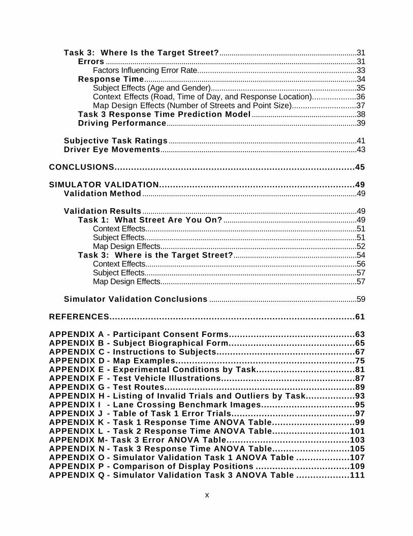
x
Task 3: Where Is the Target Street?...................................................................31Errors ...........................................................................................................................31
Factors Influencing Error Rate...........................................................................33Response Time........................................................................................................34
Subject Effects (Age and Gender)....................................................................35Context Effects (Road, Time of Day, and Response Location)....................36Map Design Effects (Number of Streets and Point Size).............................37
Task 3 Response Time Prediction Model ...................................................38Driving Performance.............................................................................................39
Subjective Task Ratings ............................................................................................41Driver Eye Movements................................................................................................43
CONCLUSIONS.......................................................................................45
SIMULATOR VALIDATION.......................................................................49Validation Method .........................................................................................................49
Validation Results .........................................................................................................49Task 1: What Street Are You On? .................................................................49
Context Effects......................................................................................................51Subject Effects......................................................................................................51Map Design Effects..............................................................................................52
Task 3: Where is the Target Street?............................................................54Context Effects......................................................................................................56Subject Effects......................................................................................................57Map Design Effects..............................................................................................57
Simulator Validation Conclusions ........................................................................59
REFERENCES.........................................................................................61
APPENDIX A - Participant Consent Forms..............................................63APPENDIX B - Subject Biographical Form..............................................65APPENDIX C - Instructions to Subjects...................................................67APPENDIX D - Map Examples.................................................................75APPENDIX E - Experimental Conditions by Task....................................81APPENDIX F - Test Vehicle Illustrations.................................................87APPENDIX G - Test Routes......................................................................89APPENDIX H - Listing of Invalid Trials and Outliers by Task..................93APPENDIX I - Lane Crossing Benchmark Images..................................95APPENDIX J - Table of Task 1 Error Trials.............................................97APPENDIX K - Task 1 Response Time ANOVA Table..............................99APPENDIX L - Task 2 Response Time ANOVA Table............................101APPENDIX M- Task 3 Error ANOVA Table............................................103APPENDIX N - Task 3 Response Time ANOVA Table............................105APPENDIX O - Simulator Validation Task 1 ANOVA Table ...................107APPENDIX P - Comparison of Display Positions ..................................109APPENDIX Q - Simulator Validation Task 3 ANOVA Table ...................111
Introduction
1
INTRODUCTION
Overview
Recently there has been an influx of in-vehicle navigation systems into the UnitedStates, both as standard equipment (on the Acura RL and several Lexus vehicles) andas aftermarket products such as the Rockwell (now Magellan) PathMaster, the Alpinevoice navigation system, and the Philips (now VDO) Carin system. A major concern isthat the in-vehicle maps provided by navigation systems may be difficult to read,distracting drivers from attending to the road ahead. Such distractions could provideincreased opportunities for crashes (Green, 1997) as is suspected for cellular phones(Goodman, Bents, Tijerina, Wierwille, Lerner, and Benel, 1997).
In recognition of this safety concern, Paul Green is developing a Society of AutomotiveEngineers (SAE) standard, a precursor to an International Standards Organization(ISO) standard, on what drivers should be permitted to do with a navigation systemwhile a vehicle is in motion. Of considerable value in developing such a standardwould be baseline data on how long it takes to read a map as a function of its contentand the task to be completed. Accordingly, this project is a timely coincidence.
There have been numerous studies concerning matters relating to human factors andthe design of navigation displays. (See Green, 1992 for a review.) Almost all of theprior research has considered issues relating to the modality to be used for navigationinformation and attentional demands of particular implementations (Dingus, McGehee,Hulse, Jahns, Manakkal, Mollenhauer, and Fleischman, 1995; Green, Hoekstra, andWilliams, 1993; Green, Williams, Hoekstra, George, and Wen, 1993), not the impact ofspecific map characteristics such as is addressed by this series of experiments.Therefore, this project breaks new ground.
The first report of this project was an annotated bibliography of the research onreading electronic area maps (Green, 1998). The report verified the a priori notion thatrelevant literature was limited. The vast majority of studies concern how colors shouldbe assigned to areas on a map (states or provinces) so no two adjacent areas havethe same color.
Several significant pilot studies were conducted as part of the first experiment. Thosestudies identified typical content of electronic maps (number of streets, street namelength, etc. for the United States) and developed a task set representative of whatdrivers do. The first major laboratory experiment, conducted in a driving simulator,examined the time to read electronic maps as a function of numerous map displayfactors (Green, 1998). A total of 20 drivers (10 under 30 years of age and 10 over 65years of age) operated a driving simulator while performing one of three tasks: (1)identifying the street being driven, (2) identifying a particular cross street, or (3)locating a particular street on a map. These same three representative tasks havebeen used consistently in this project. Further, they are interesting experimentally asthey vary in complexity and completion time.
Introduction
2
Variables examined in the first experiment included: (1) the number of streets shown(6 through 36), (2) label point size (12 and 18 point), (3) the street configuration (gridverses nongrid), and (4) the street label orientation (horizontal, vertical, and verticalstacked).
The results were that the response times increased as the number of streets shownincreased. For the label size, the reading time for 18 point text was significantly slower(by 11 percent) than for 12 point, especially with a large number of streets on the map.Large point sizes combined with many visible streets created a cluttered map whichdramatically increased the drivers’ response times. Additionally, drivers were able toread the maps faster when the maps were based on a grid layout, rather than a lessstructured, more random arrangement. The regularity of the grid facilitated search.Finally, the best label orientations were horizontal for horizontal streets and vertical forvertical streets, even though horizontal text is normally easier to read. In this case, thevertical text facilitated the association of each label with a particular line representing astreet.
Following the initial laboratory experiment, a second laboratory experiment wasconducted in parallel with this on-the-road study to reexamine some of the mapdisplay factors (Brooks and Green, 1998). Using the same three tasks as the firstexperiment, the variables examined in the second experiment included: (1) thenumber of streets (12 through 36), (2) label point size (10, 12, and 14 point), (3)percentage of streets labeled (33, 66, 100 percent), (4) display location (high or low onthe center console).
The results of the second laboratory experiment showed that labeled streets increasedthe response times more than the unlabeled streets for most of the tasks, and amaximum of 12 labeled streets should be used on the map to optimize searchperformance. The experiment also found that the use of 10 point text increased theresponse times for all tasks, especially for older drivers. In general 14 point text waspreferred, although clutter effects were seen when using that point size on mapscontaining more than 16 labeled streets. The effect of display location was only testedusing the first task, identify the street being driven. The higher location producedslightly faster response times (by 10 percent).
Issues
All of the initial work was conducted in a driving simulator to provide consistent testconditions and reduce cost. However, once the relationships of the key factors wereestablished, it was necessary to determine the necessary adjustment of the laboratorydata to predict on-the-road performance. Consequently, some of the test conditionsfrom the previous simulator study (plus some additional conditions of interest) wereexplored on the road.
Introduction
3
There were four key issues:
1. When do drivers feel that map reading is unsafe while driving?
Maps should not be so complex that they require an excessively long time to read. Themajor concern is that if drivers are not looking at the road, the risk of a crash increases.Prior to this research, there was a minimum of data on what drivers thought to beexcessive. (See Hada, 1994 as an example.) One way to determine when driversbegan to feel uncomfortable was to ask them to rate the tasks on a scale with regard tointerference with driving and perceived safety.
2. What size text and how many streets should be displayed?
The first experiment tested only 12- and 18-point text sizes for street names, both ofwhich are larger than the text used in some U.S. navigation systems. Unresolved wasthe impact of smaller font sizes on map reading times. Since the first experimentshowed a large street’s effect and an interaction between streets and text size, thenumber of streets displayed was also included as a factor in the on-the-roadexperiment.
3. How does the ambient lighting (time of day) affect map reading?
Altering the ambient light changes both the display contrast and its overall luminancelevel. The lighting levels in the UMTRI simulator approximated dusk. Although someadjustments can be made, limits of the scene projector output make simulating a widerange of conditions, especially daylight, difficult. (This is true of all driving simulators ofwhich the authors are aware.) Accordingly, on-road driving was used to examine theeffects of ambient lighting. Readers should remember that changes in sceneluminance and interior illumination occur together, and furthermore, day-nightdifferences were accompanied by changes in traffic volume.
4. How do the simulator results compare with the on-the-road results?
Experiments were conducted, for the most part, in the driving simulator because theconditions could be well controlled, especially traffic, leading to more stable results.Further, Michigan winters made collecting on-the-road data impossible. Rain in thespring and fall can likewise be problematic leading to schedule delays. Since the datawas collected to predict on-the-road performance, differences between the twocontexts were examined experimentally by replicating a subset of the test conditionsfrom the driving-simulator experiment in the on-the-road experiment.
As an aside, the fourth experiment, which is in the planning stages as this report isbeing written, will consider when drivers want maps and when turn displays should beprovided. The rationale is that for reasons of space and cost, only a single displaymay be available. The ideal situation would be for the navigation computer to "know"at any given moment which display format a driver might desire, and automaticallypresent it, rather that forcing a driver to press a key each time a different format displayshould appear.

4
Test Plan
5
TEST PLAN
Test Participants
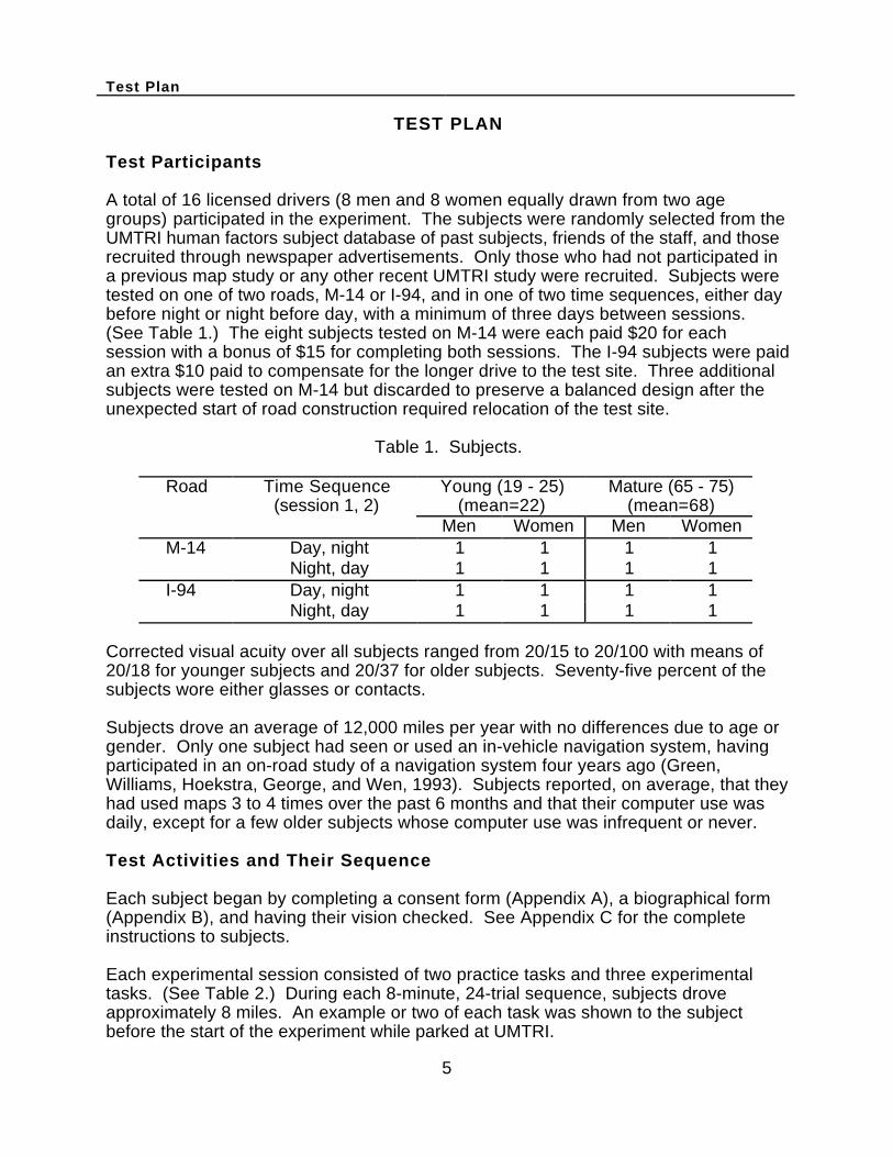
A total of 16 licensed drivers (8 men and 8 women equally drawn from two agegroups) participated in the experiment. The subjects were randomly selected from theUMTRI human factors subject database of past subjects, friends of the staff, and thoserecruited through newspaper advertisements. Only those who had not participated ina previous map study or any other recent UMTRI study were recruited. Subjects weretested on one of two roads, M-14 or I-94, and in one of two time sequences, either daybefore night or night before day, with a minimum of three days between sessions.(See Table 1.) The eight subjects tested on M-14 were each paid $20 for eachsession with a bonus of $15 for completing both sessions. The I-94 subjects were paidan extra $10 paid to compensate for the longer drive to the test site. Three additionalsubjects were tested on M-14 but discarded to preserve a balanced design after theunexpected start of road construction required relocation of the test site.
Table 1. Subjects.
Road Time Sequence(session 1, 2)
Young (19 - 25)(mean=22)
Mature (65 - 75)(mean=68)
Men Women Men WomenM-14 Day, night 1 1 1 1
Night, day 1 1 1 1I-94 Day, night 1 1 1 1
Night, day 1 1 1 1
Corrected visual acuity over all subjects ranged from 20/15 to 20/100 with means of20/18 for younger subjects and 20/37 for older subjects. Seventy-five percent of thesubjects wore either glasses or contacts.
Subjects drove an average of 12,000 miles per year with no differences due to age orgender. Only one subject had seen or used an in-vehicle navigation system, havingparticipated in an on-road study of a navigation system four years ago (Green,Williams, Hoekstra, George, and Wen, 1993). Subjects reported, on average, that theyhad used maps 3 to 4 times over the past 6 months and that their computer use wasdaily, except for a few older subjects whose computer use was infrequent or never.
Test Activities and Their Sequence
Each subject began by completing a consent form (Appendix A), a biographical form(Appendix B), and having their vision checked. See Appendix C for the completeinstructions to subjects.
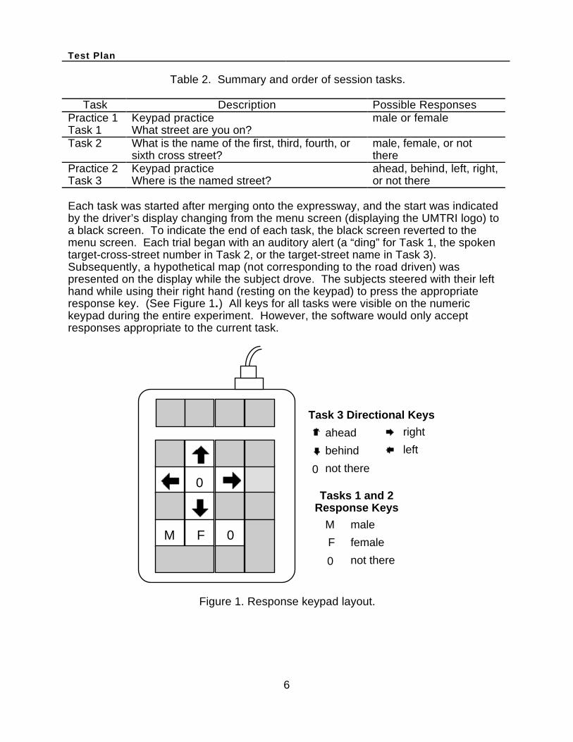
Each experimental session consisted of two practice tasks and three experimentaltasks. (See Table 2.) During each 8-minute, 24-trial sequence, subjects droveapproximately 8 miles. An example or two of each task was shown to the subjectbefore the start of the experiment while parked at UMTRI.
Test Plan
6
Table 2. Summary and order of session tasks.
Task Description Possible ResponsesPractice 1 Keypad practice male or femaleTask 1 What street are you on?Task 2 What is the name of the first, third, fourth, or
sixth cross street?male, female, or notthere
Practice 2 Keypad practice ahead, behind, left, right,Task 3 Where is the named street? or not there
Each task was started after merging onto the expressway, and the start was indicatedby the driver’s display changing from the menu screen (displaying the UMTRI logo) toa black screen. To indicate the end of each task, the black screen reverted to themenu screen. Each trial began with an auditory alert (a “ding” for Task 1, the spokentarget-cross-street number in Task 2, or the target-street name in Task 3).Subsequently, a hypothetical map (not corresponding to the road driven) waspresented on the display while the subject drove. The subjects steered with their lefthand while using their right hand (resting on the keypad) to press the appropriateresponse key. (See Figure 1.) All keys for all tasks were visible on the numerickeypad during the entire experiment. However, the software would only acceptresponses appropriate to the current task.
M F 0
0
behind
ahead
left
right
not there
male
female
not there
Task 3 Directional Keys
Tasks 1 and 2Response Keys
0
M
F
0
Figure 1. Response keypad layout.
Test Plan
7
Response times (measured to 1/60 of a second) and errors were recorded. If thesubject answered correctly, the computer played a “beep.” If the subject answeredincorrectly or failed to answer within 25 seconds, the computer played a “buzz.” Thewhole process repeated after an intertrial interval (ITI) randomly chosen between 10and 12 seconds (in half-second increments). The intertrial interval was intended toallow sufficient time for drivers to recover from a trial and refocus their attention todriving. During the ITI the experimenter was able to pause the experiment, leading toa few trials (12 percent) with irregular ITI’s ranging from 3 to 57 seconds. Theexperimenter paused the experiment whenever something occurred that wouldinterfere with the subject's response such as subject questions, removing their handfrom the keypad, or disruptive traffic (police car, tow truck, road obstruction, mergingvehicle, and passing a slow-moving vehicle).
Map Construction
The maps were based on 4 street-templates. Maps contained either 12 or 24 streets.The 12-street maps were made by deleting 12 of the 24 streets on a 24-street map,thus resembling a “zoomed out” version of the 24-street map. Street labels wereprinted in 10-, 12-, or 14-point Helvetica. Street labels were oriented horizontally forhorizontal streets and vertically for vertical streets as per the results of a previousexperiment. Based on prior work to develop representative maps for the UnitedStates, all maps were based on a grid design containing one railroad and one river.All street names were common, unambiguously male or female names (according to a"baby book," Evans, 1994) ranging from 5 to 9 characters (lengths typical of US streetnames). Appendix D contains a sample of the maps used in this experiment and adiscussion of the response time differences found between map templates. Topartially counterbalance for order effects, each task contained a set of 24 trials (24unique maps) shown in a fixed random sequence with each subject starting at 1 of 5different points.
Task Descriptions
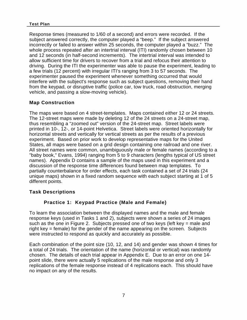
Practice 1: Keypad Practice (Male and Female)
To learn the association between the displayed names and the male and femaleresponse keys (used in Tasks 1 and 2), subjects were shown a series of 24 imagessuch as the one in Figure 2. Subjects pressed one of two keys (left key = male andright key = female) for the gender of the name appearing on the screen. Subjectswere instructed to respond as quickly and accurately as possible.
Each combination of the point size (10, 12, and 14) and gender was shown 4 times fora total of 24 trials. The orientation of the name (horizontal or vertical) was randomlychosen. The details of each trial appear in Appendix E. Due to an error on one 14-point slide, there were actually 5 replications of the male response and only 3replications of the female response instead of 4 replications each. This should haveno impact on any of the results.
Test Plan
8
DO
UG
LA
S
Figure 2. Practice 1. Example: The subject reads“DOUGLAS” and responds by pressing the “male” key.
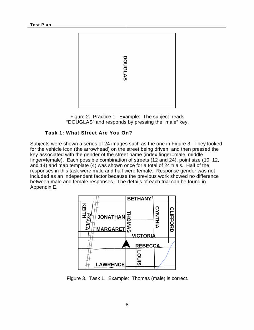
Task 1: What Street Are You On?
Subjects were shown a series of 24 images such as the one in Figure 3. They lookedfor the vehicle icon (the arrowhead) on the street being driven, and then pressed thekey associated with the gender of the street name (index finger=male, middlefinger=female). Each possible combination of streets (12 and 24), point size (10, 12,and 14) and map template (4) was shown once for a total of 24 trials. Half of theresponses in this task were male and half were female. Response gender was notincluded as an independent factor because the previous work showed no differencebetween male and female responses. The details of each trial can be found inAppendix E.
TH
OM
AS
BETHANY
JONATHAN
PA
UL
A
CL
IFF
OR
D
VICTORIA
KE
ITH
LAWRENCE
CY
NT
HIA
LO
UIS
REBECCA
MARGARET
Figure 3. Task 1. Example: Thomas (male) is correct.
Test Plan
9
Task 2: What Is the nth Cross Street?
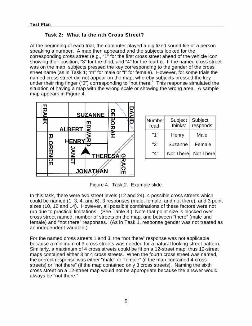
At the beginning of each trial, the computer played a digitized sound file of a personspeaking a number. A map then appeared and the subjects looked for thecorresponding cross street (e.g., “1” for the first cross street ahead of the vehicle iconshowing their position, “3” for the third, and “4” for the fourth). If the named cross streetwas on the map, subjects pressed the key corresponding to the gender of the crossstreet name (as in Task 1; “m” for male or “f” for female). However, for some trials thenamed cross street did not appear on the map, whereby subjects pressed the keyunder their ring finger (“0”) corresponding to “not there.” This response simulated thesituation of having a map with the wrong scale or showing the wrong area. A samplemap appears in Figure 4.
GR
AC
EJONATHAN
FR
AN
K SUZANNE
DE
BO
RA
HFL
OR
EN
CE
HENRY
ED
WA
RD
THERESA
ALBERT
JAN
ET
DA
VID Number
readSubject thinks:
Subjectresponds:
"1" Henry Male
"3" Suzanne Female
"4" Not There Not There
Figure 4. Task 2. Example slide.
In this task, there were two street levels (12 and 24), 4 possible cross streets whichcould be named (1, 3, 4, and 6), 3 responses (male, female, and not there), and 3 pointsizes (10, 12 and 14). However, all possible combinations of these factors were notrun due to practical limitations. (See Table 3.) Note that point size is blocked overcross street named, number of streets on the map, and between “there” (male andfemale) and “not there” responses. (As in Task 1, response gender was not treated asan independent variable.)
For the named cross streets 1 and 3, the “not there” response was not applicablebecause a minimum of 3 cross streets was needed for a natural looking street pattern.Similarly, a maximum of 4 cross streets could be fit on a 12-street map; thus 12-streetmaps contained either 3 or 4 cross streets. When the fourth cross street was named,the correct response was either “male” or “female” (if the map contained 4 crossstreets) or “not there” (if the map contained only 3 cross streets). Naming the sixthcross street on a 12-street map would not be appropriate because the answer wouldalways be “not there.”
Test Plan
10
Table 3. Number of Task 2 trials per combination of cross street named, number of streets, and correct response.
12-Street Maps 24-Street Maps Cross Street Correct Response Correct Response
Named Male Female
NotThere
Male Female
Not There
1 0 3 N/A 1 2 N/A3 2 1 N/A 3 0 N/A4 1 2 3 N/A N/A N/A6 N/A N/A N/A 2 1 3
In order to look natural, the 24-street maps contained either 5 or 6 cross streets. Whenthe sixth cross street was named, the correct response was either “male” or “female” (ifthe map contained 6 cross streets) or “not there” (if the map contained only 5 crossstreets). The fourth cross street was not tested on a 24-street map due to the limitedamount of driving time during the task. Details of the experimental conditions can befound in Appendix E.
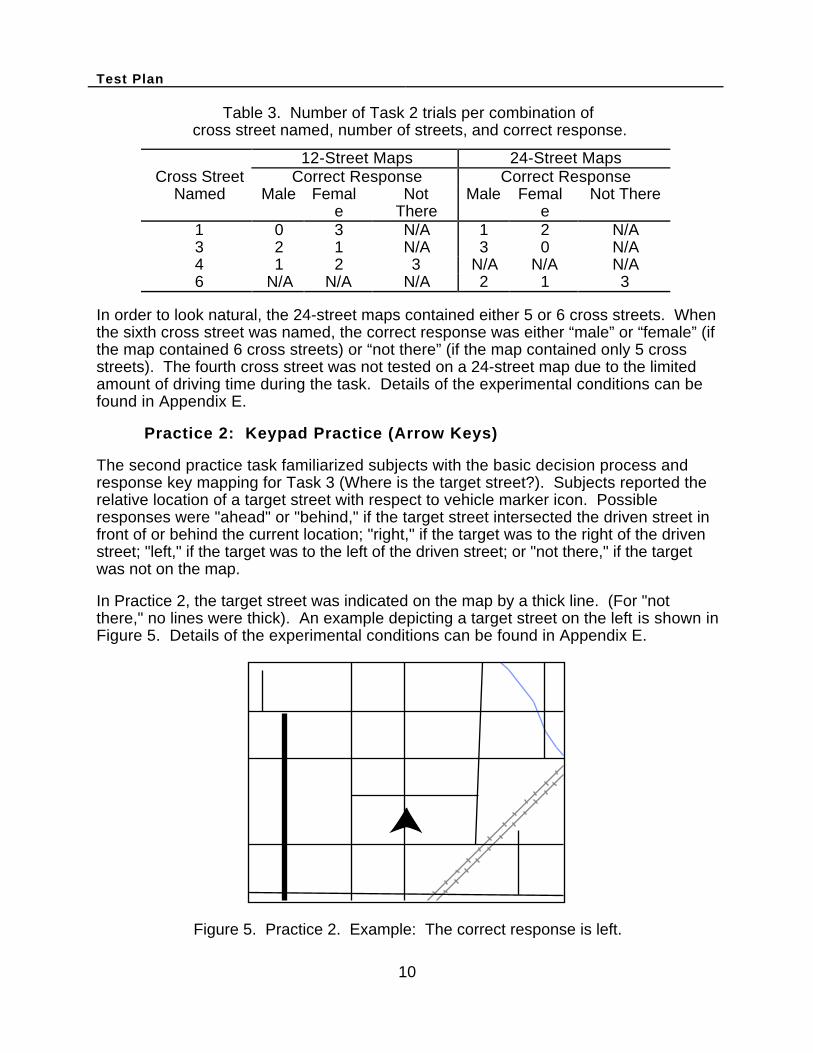
Practice 2: Keypad Practice (Arrow Keys)
The second practice task familiarized subjects with the basic decision process andresponse key mapping for Task 3 (Where is the target street?). Subjects reported therelative location of a target street with respect to vehicle marker icon. Possibleresponses were "ahead" or "behind," if the target street intersected the driven street infront of or behind the current location; "right," if the target was to the right of the drivenstreet; "left," if the target was to the left of the driven street; or "not there," if the targetwas not on the map.
In Practice 2, the target street was indicated on the map by a thick line. (For "notthere," no lines were thick). An example depicting a target street on the left is shown inFigure 5. Details of the experimental conditions can be found in Appendix E.
Figure 5. Practice 2. Example: The correct response is left.
Test Plan
11
Task 3: Where Is the Target Street?
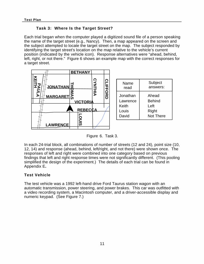
Each trial began when the computer played a digitized sound file of a person speakingthe name of the target street (e.g., Nancy). Then, a map appeared on the screen andthe subject attempted to locate the target street on the map. The subject responded byidentifying the target street's location on the map relative to the vehicle’s currentposition (indicated by the vehicle icon). Response alternatives were “ahead, behind,left, right, or not there.” Figure 6 shows an example map with the correct responses fora target street.
TH
OM
AS
BETHANY
JONATHAN
PA
UL
A
CL
IFF
OR
DVICTORIA
KE
ITH
LAWRENCE
CY
NT
HIA
LO
UIS
REBECCA
MARGARET
Name read
Subjectanswers:
Jonathan
Louis
LawrenceKeith
David
AheadBehindLeftRightNot There
Figure 6. Task 3.
In each 24-trial block, all combinations of number of streets (12 and 24), point size (10,12, 14) and response (ahead, behind, left/right, and not there) were shown once. Theresponses of left and right were combined into one category based on previousfindings that left and right response times were not significantly different. (This poolingsimplified the design of the experiment.) The details of each trial can be found inAppendix E.
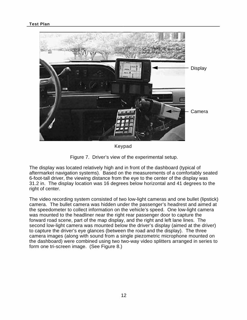
Test Vehicle
The test vehicle was a 1992 left-hand drive Ford Taurus station wagon with anautomatic transmission, power steering, and power brakes. This car was outfitted witha video recording system, a Macintosh computer, and a driver-accessible display andnumeric keypad. (See Figure 7.)
Test Plan
12
Keypad
Camera
Display
Figure 7. Driver’s view of the experimental setup.
The display was located relatively high and in front of the dashboard (typical ofaftermarket navigation systems). Based on the measurements of a comfortably seated6-foot-tall driver, the viewing distance from the eye to the center of the display was31.2 in. The display location was 16 degrees below horizontal and 41 degrees to theright of center.
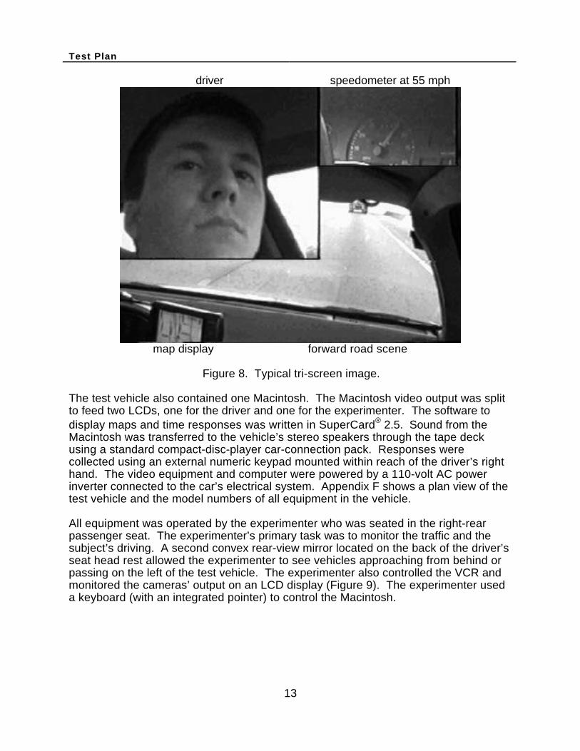
The video recording system consisted of two low-light cameras and one bullet (lipstick)camera. The bullet camera was hidden under the passenger’s headrest and aimed atthe speedometer to collect information on the vehicle’s speed. One low-light camerawas mounted to the headliner near the right rear passenger door to capture theforward road scene, part of the map display, and the right and left lane lines. Thesecond low-light camera was mounted below the driver’s display (aimed at the driver)to capture the driver’s eye glances (between the road and the display). The threecamera images (along with sound from a single piezometric microphone mounted onthe dashboard) were combined using two two-way video splitters arranged in series toform one tri-screen image. (See Figure 8.)
Test Plan
13
driver speedometer at 55 mph
map display forward road scene
Figure 8. Typical tri-screen image.
The test vehicle also contained one Macintosh. The Macintosh video output was splitto feed two LCDs, one for the driver and one for the experimenter. The software todisplay maps and time responses was written in SuperCard® 2.5. Sound from theMacintosh was transferred to the vehicle’s stereo speakers through the tape deckusing a standard compact-disc-player car-connection pack. Responses werecollected using an external numeric keypad mounted within reach of the driver’s righthand. The video equipment and computer were powered by a 110-volt AC powerinverter connected to the car’s electrical system. Appendix F shows a plan view of thetest vehicle and the model numbers of all equipment in the vehicle.
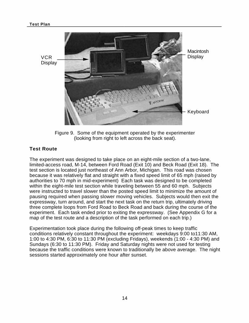
All equipment was operated by the experimenter who was seated in the right-rearpassenger seat. The experimenter’s primary task was to monitor the traffic and thesubject’s driving. A second convex rear-view mirror located on the back of the driver’sseat head rest allowed the experimenter to see vehicles approaching from behind orpassing on the left of the test vehicle. The experimenter also controlled the VCR andmonitored the cameras’ output on an LCD display (Figure 9). The experimenter useda keyboard (with an integrated pointer) to control the Macintosh.
Test Plan
14
MacintoshDisplayVCR
Display
Keyboard
Figure 9. Some of the equipment operated by the experimenter(looking from right to left across the back seat).
Test Route
The experiment was designed to take place on an eight-mile section of a two-lane,limited-access road, M-14, between Ford Road (Exit 10) and Beck Road (Exit 18). Thetest section is located just northeast of Ann Arbor, Michigan. This road was chosenbecause it was relatively flat and straight with a fixed speed limit of 65 mph (raised byauthorities to 70 mph in mid-experiment) Each task was designed to be completedwithin the eight-mile test section while traveling between 55 and 60 mph. Subjectswere instructed to travel slower than the posted speed limit to minimize the amount ofpausing required when passing slower moving vehicles. Subjects would then exit theexpressway, turn around, and start the next task on the return trip, ultimately drivingthree complete loops from Ford Road to Beck Road and back during the course of theexperiment. Each task ended prior to exiting the expressway. (See Appendix G for amap of the test route and a description of the task performed on each trip.)
Experimentation took place during the following off-peak times to keep trafficconditions relatively constant throughout the experiment: weekdays 9:00 to11:30 AM,1:00 to 4:30 PM, 6:30 to 11:30 PM (excluding Fridays), weekends (1:00 - 4:30 PM) andSundays (6:30 to 11:30 PM). Friday and Saturday nights were not used for testingbecause the traffic conditions were known to traditionally be above average. The nightsessions started approximately one hour after sunset.
Test Plan
15
The experiment also took place only in good weather (no rain, snow, ice, or fog).Sessions that were canceled due to bad weather were rescheduled. Severalsessions did encounter unexpected light drizzle or rain for part of a task, at which timethe subject had the option of continuing. If the rain became hard enough to requireconstant use of the windshield wipers, the experiment was paused for several minutesto wait out the rain.
Unknown in advance, the Michigan Department of Transportation announced plans toclose the M-14 segment for repairs while testing was in progress. Sinceapproximately half of the testing had been completed, the experimental design wasaltered to allow for testing on a second road similar to M-14. A second test routesegment on I-94 between Baker Road (Exit 167) and US 52 (Exit 159) was selected.The I-94 segment was actually less curvy than the M-14 route, but it contained moregrade changes (hills). While this should not affect the response time in the map-reading task, more lane crossings were expected on M-14, and greater speeddeviations were expected on I-94. The same procedure of running one task per eight-mile trip was used on the I-94 segment. (See Appendix G for a map of the test routeand a description of the task performed on each trip.)
The I-94 route was also chosen because of its similarity in traffic volume to M-14.Traffic on I-94 (annual average daily traffic 49,460 vehicles) was only slightly heavierthan the traffic on M-14 (annual average daily traffic 47,003 vehicles). However, the I-94 traffic contained more trucks (approximately 35 percent of the traffic volume versus17 percent of the M-14 traffic). For both routes, the day sessions experiencedapproximately twice the hourly volume of traffic as night sessions.

16

Results Data Reduction
17
RESULTS
Data Reduction
Four performance measures were independently analyzed in this experiment:(1) response time, (2) response errors, (3) lane excursions, and (4) unintentionalinstances of speed decrease. Response time and response errors were recorded bythe software written to display the maps. Lane excursions and speed decreases wereobtained from a slow speed playback of the session videotapes using a frame-accurate VCR. Additionally while watching the session videotapes for lane excursionsand speed decreases, the analyst recorded the number of glances between theroadway and the display while a map was being shown for each trial.
Response time was defined as the time (measured in ticks or sixtieths of a second)between a map’s appearance and when the subject pressed a key on the keypad.Any response faster than 150 ms was automatically disregarded as accidentalkeystrokes, and the subject was allowed to continue the trial and respond a secondtime. Based on the quickest response times seen in previous experiments, responsesbetween 150 ms and 400 ms were flagged as being possibly too fast, but the trial wascounted as completed. Only one response in this category occurred during theexperiment and the subject immediately confirmed that the keystroke wasunintentional.
The analyst also noted response times which were possibly suspect because thesubject (1) was not ready for the trial to begin (e.g., asked a question during the trial ormoved his or her hand from the keypad); (2) was distracted by traffic; or (3) could nothear or understand the number (Task 2) or name (Task 3) of the target street as it wasread. Suspect response times were replaced with a mean if the specific response timewas an outlier. (An outlier was defined as any trial response time which exceeded thesubject’s task mean response time plus 4 times the standard deviation.)
There were initially no suspect trials in Task 1, but further analysis revealed 2 outliersin excess of 10 seconds which were replaced by the subject’s average response timefor similar point size and street level across the 4 map templates. (Note: Each taskcontained 768 trials.) In Task 2, there were six suspect trials, 3 of which wereconsidered outliers and replaced with the subject’s average response time acrosspoint size for a similar number of streets and cross street named. In Task 3, there wereno outliers and none of the five suspect trials were replaced. A list of trials removed iscontained in Appendix H.
A response error was defined as whether or not the subject answered the trialcorrectly. Where possible, the experimenter noted the any obvious explanations foreach error or any subject comments. (Sometimes the subjects would explain thereason for the error immediately following the trial such as saying, “I hit the wrong key,”or, “I really meant to a press....”)
There were two driving performance measures: lane excursions and unintendedspeed decreases. Lane excursions occurred when drivers paid excessive attention tothe map display (diverting attention from steering) and allowed the vehicle to crosseither the left- or right-lane marker. Because the experimenter was constantly

Results Data Reduction
18
monitoring the traffic and the subject’s driving, there was minimal risk when laneexcursions occurred. To assist in judging when lane excursions occurred, the forward-looking camera was positioned to capture both edge lane lines for the lane driven.The videotaped image was then compared to two reference images showing thevehicle at the threshold of crossing the lane marker. (See Appendix I.)
Unintended speed decreases were characterized by a constant speed decreaseduring the trial while the subject attended to the map followed by a rapid accelerationafter the trial when the subject realized that their speed had dropped. In the videoanalysis, the speedometer camera was used to judge the speed drop during the trials(only decreases greater than 3 mph could be accurately detected using this method).Some speed losses were due to nonexperimental factors evident in the video (such astraffic slowing ahead) and were not counted as an unintended speed decrease.
Task 1: What Street Are You On?
Errors
The overall task error rate was 1.8 percent (14 out of 768 trials). The few errors appearrandom and are described in Appendix J. Several subjects reported confusionbetween the name Michelle and Michael, but neither name was missed more thanwould be expected due to random errors.
Response Time
The response times for Task 1 ranged from 933 to 7000 ms with a mean of 1790 ms(standard deviation = 690 ms). Figure 10 shows the distribution and the cumulativedistribution of response times measured during this task. Ninety-five percent of theresponse times were under approximately 3 seconds.
0
5
10
15
20
Fre
quen
cy (
Per
cent
age)
0 1 2 3 4 5 6 7 8Response Time (s)
Cum
ulat
ive
(Per
cent
age)
10
20
30
40
50
60
70
80
90
100
Figure 10. Task 1: Distribution of response times.
Results Task 1
19
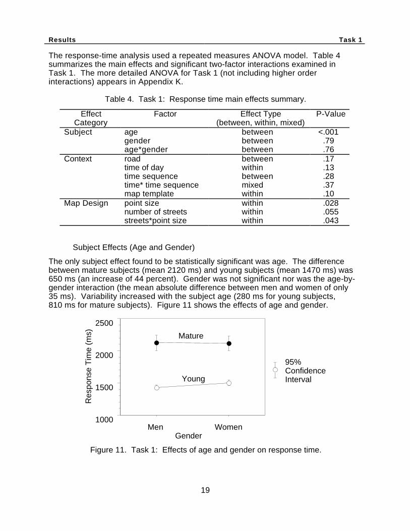
The response-time analysis used a repeated measures ANOVA model. Table 4summarizes the main effects and significant two-factor interactions examined inTask 1. The more detailed ANOVA for Task 1 (not including higher orderinteractions) appears in Appendix K.
Table 4. Task 1: Response time main effects summary.
EffectCategory
Factor Effect Type(between, within, mixed)
P-Value
Subject age between <.001gender between .79age*gender between .76
Context road between .17time of day within .13time sequence between .28time* time sequence mixed .37map template within .10
Map Design point size within .028number of streets within .055streets*point size within .043
Subject Effects (Age and Gender)
The only subject effect found to be statistically significant was age. The differencebetween mature subjects (mean 2120 ms) and young subjects (mean 1470 ms) was650 ms (an increase of 44 percent). Gender was not significant nor was the age-by-gender interaction (the mean absolute difference between men and women of only35 ms). Variability increased with the subject age (280 ms for young subjects,810 ms for mature subjects). Figure 11 shows the effects of age and gender.
1000
1500
2000
2500
Res
pons
e T
ime
(ms)
Men WomenGender
Mature
Young
95%ConfidenceInterval
Figure 11. Task 1: Effects of age and gender on response time.
Results Task 1
20
Context Effects (Road, Time of Day, and Map Template)
The effects of map template (a maximum difference between any two templates of 125ms) and road (a 95 ms difference) were not found to be significant; however, a moredetailed discussion of each effect can be found in Appendix D and G, respectively.
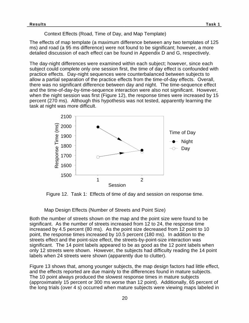
The day-night differences were examined within each subject; however, since eachsubject could complete only one session first, the time of day effect is confounded withpractice effects. Day-night sequences were counterbalanced between subjects toallow a partial separation of the practice effects from the time-of-day effects. Overall,there was no significant difference between day and night. The time-sequence effectand the time-of-day-by-time-sequence interaction were also not significant. However,when the night session was first (Figure 12), the response times were increased by 15percent (270 ms). Although this hypothesis was not tested, apparently learning thetask at night was more difficult.
Night
1500
1600
1700
1800
1900
2000
2100
Res
pons
e T
ime
(ms)
1 2Session
Day
Time of Day
Figure 12. Task 1: Effects of time of day and session on response time.
Map Design Effects (Number of Streets and Point Size)
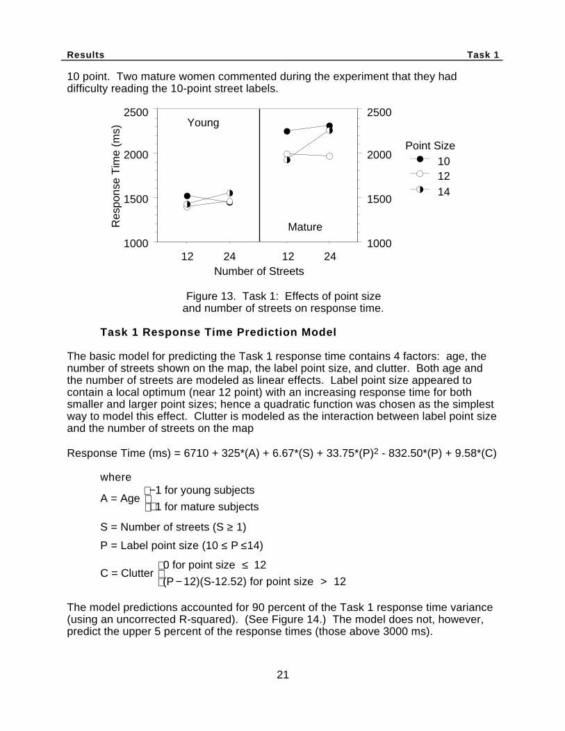
Both the number of streets shown on the map and the point size were found to besignificant. As the number of streets increased from 12 to 24, the response timeincreased by 4.5 percent (80 ms). As the point size decreased from 12 point to 10point, the response times increased by 10.5 percent (180 ms). In addition to thestreets effect and the point-size effect, the streets-by-point-size interaction wassignificant. The 14 point labels appeared to be as good as the 12 point labels whenonly 12 streets were shown. However, the subjects had difficulty reading the 14 pointlabels when 24 streets were shown (apparently due to clutter).
Figure 13 shows that, among younger subjects, the map design factors had little effect,and the effects reported are due mainly to the differences found in mature subjects.The 10 point always produced the slowest response times in mature subjects(approximately 15 percent or 300 ms worse than 12 point). Additionally, 65 percent ofthe long trials (over 4 s) occurred when mature subjects were viewing maps labeled in
Results Task 1
21
10 point. Two mature women commented during the experiment that they haddifficulty reading the 10-point street labels.
1000
1500
2000
2500R
espo
nse
Tim
e (m
s)
12 24 12 24
Young
Mature
141210
Point Size
Number of Streets
1000
1500
2000
2500
Figure 13. Task 1: Effects of point sizeand number of streets on response time.
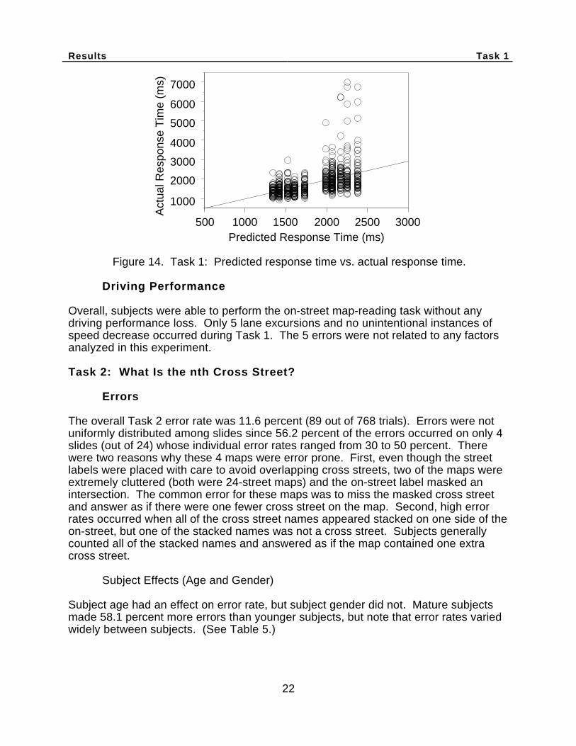
Task 1 Response Time Prediction Model
The basic model for predicting the Task 1 response time contains 4 factors: age, thenumber of streets shown on the map, the label point size, and clutter. Both age andthe number of streets are modeled as linear effects. Label point size appeared tocontain a local optimum (near 12 point) with an increasing response time for bothsmaller and larger point sizes; hence a quadratic function was chosen as the simplestway to model this effect. Clutter is modeled as the interaction between label point sizeand the number of streets on the map
Response Time (ms) = 6710 + 325*(A) + 6.67*(S) + 33.75*(P)2 - 832.50*(P) + 9.58*(C)
where
A = Age −1 for young subjects
+1 for mature subjects
S = Number of streets (S ≥ 1)
P = Label point size (10 ≤ P ≤14)
C = Clutter 0 for point size ≤ 12
(P − 12)(S-12.52) for point size > 12
The model predictions accounted for 90 percent of the Task 1 response time variance(using an uncorrected R-squared). (See Figure 14.) The model does not, however,predict the upper 5 percent of the response times (those above 3000 ms).
Results Task 1
22
500 1000 1500 2000 2500 3000
Act
ual R
espo
nse
Tim
e (m
s)
Predicted Response Time (ms)
1000
2000
3000
4000
5000
6000
7000
Figure 14. Task 1: Predicted response time vs. actual response time.
Driving Performance
Overall, subjects were able to perform the on-street map-reading task without anydriving performance loss. Only 5 lane excursions and no unintentional instances ofspeed decrease occurred during Task 1. The 5 errors were not related to any factorsanalyzed in this experiment.
Task 2: What Is the nth Cross Street?
Errors
The overall Task 2 error rate was 11.6 percent (89 out of 768 trials). Errors were notuniformly distributed among slides since 56.2 percent of the errors occurred on only 4slides (out of 24) whose individual error rates ranged from 30 to 50 percent. Therewere two reasons why these 4 maps were error prone. First, even though the streetlabels were placed with care to avoid overlapping cross streets, two of the maps wereextremely cluttered (both were 24-street maps) and the on-street label masked anintersection. The common error for these maps was to miss the masked cross streetand answer as if there were one fewer cross street on the map. Second, high errorrates occurred when all of the cross street names appeared stacked on one side of theon-street, but one of the stacked names was not a cross street. Subjects generallycounted all of the stacked names and answered as if the map contained one extracross street.
Subject Effects (Age and Gender)
Subject age had an effect on error rate, but subject gender did not. Mature subjectsmade 58.1 percent more errors than younger subjects, but note that error rates variedwidely between subjects. (See Table 5.)

Results Task 2
23
Table 5. Task 2: Number of errors per subject.
Age Gender Subject ResponseTime (ms)
Number ofErrors
Male 1 2080 42 2730 43 3100 2
Young 4 3110 4Female 1 3390 2
2 2350 23 2730 64 2850 5
Male 1 3890 82 4120 93 3460 6
Mature 4 4230 10Female 1 4010 9
2 3130 53 2950 44 4720 9
There is a statistically significant correlation (p < .001) between the subjects’response times and error rates (r = .79). To determine if all subjects were performingat a similar trade-off between speed and accuracy (i.e., some subjects were notsacrificing accuracy for fast response times), a speed-accuracy operatingcharacteristic curve was computed for the pool of test subjects. (See Figure 15.)Subject performance could generally be classified as either good (fast response timesand high accuracy) or poor (slow response times and low accuracy) with more of themature subjects falling into the later category.
Mature
Young
Age
.5
.6
.7
.8
.91
1.11.21.31.41.5
2 3 4 5Response Time (s)
logP(correct)
P(error)[ ]SpeedStress
AccuracyStress
Good
Poor
Accuracy
Figure 15. Task 2: Speed-accuracy operating characteristics across subjects.
Results Task 2
24
Context Effects
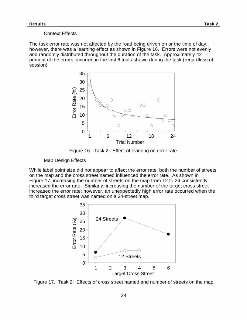
The task error rate was not affected by the road being driven on or the time of day,however, there was a learning effect as shown in Figure 16. Errors were not evenlyand randomly distributed throughout the duration of the task. Approximately 42percent of the errors occurred in the first 6 trials shown during the task (regardless ofsession).
0
5
10
15
20
25
30
35E
rror
Rat
e (%
)
Trial Number1 6 12 18 24
Figure 16. Task 2: Effect of learning on error rate.
Map Design Effects
While label point size did not appear to affect the error rate, both the number of streetson the map and the cross street named influenced the error rate. As shown inFigure 17, increasing the number of streets on the map from 12 to 24 consistentlyincreased the error rate. Similarly, increasing the number of the target cross streetincreased the error rate; however, an unexpectedly high error rate occurred when thethird target cross street was named on a 24-street map.
Err
or R
ate
(%)
1 2 3 4 5 6Target Cross Street
24 Streets
12 Streets0
5
10
15
20
25
30
35
Figure 17. Task 2: Effects of cross street named and number of streets on the map.
Results Task 2
25
Response Time
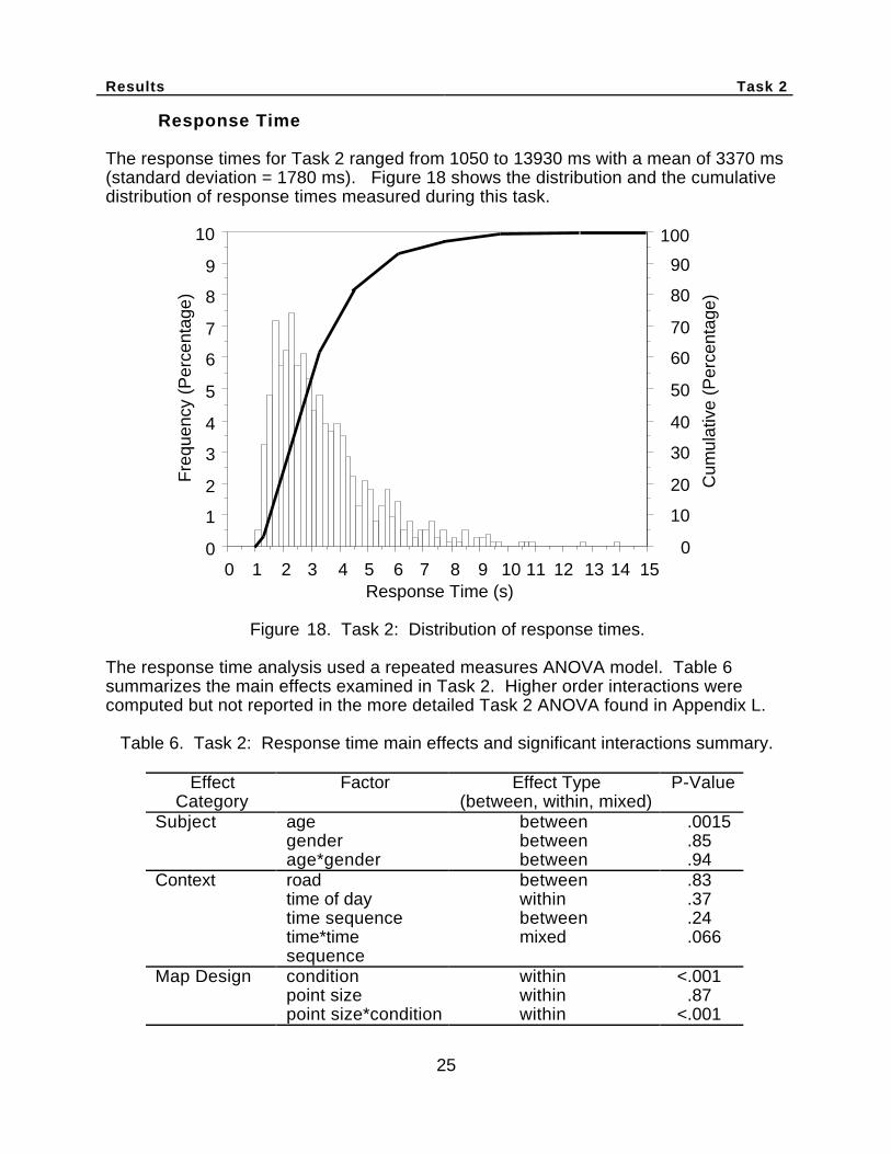
The response times for Task 2 ranged from 1050 to 13930 ms with a mean of 3370 ms(standard deviation = 1780 ms). Figure 18 shows the distribution and the cumulativedistribution of response times measured during this task.
Fre
quen
cy (
Per
cent
age)
0 2 4 6 8 10 12 14Response Time (s)
1 3 5 7 9 11 13 150
10
20
30
40
50
60
70
80
90
100
Cum
ulat
ive
(Per
cent
age)
0
1
2
3
4
5
6
7
8
9
10
Figure 18. Task 2: Distribution of response times.
The response time analysis used a repeated measures ANOVA model. Table 6summarizes the main effects examined in Task 2. Higher order interactions werecomputed but not reported in the more detailed Task 2 ANOVA found in Appendix L.
Table 6. Task 2: Response time main effects and significant interactions summary.
EffectCategory
Factor Effect Type(between, within, mixed)
P-Value
Subject age between .0015gender between .85age*gender between .94
Context road between .83time of day within .37time sequence between .24time*timesequence
mixed .066
Map Design condition within <.001point size within .87point size*condition within <.001
Results Task 2
26
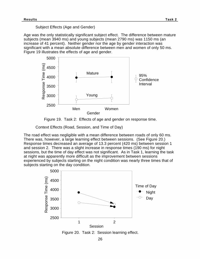
Subject Effects (Age and Gender)
Age was the only statistically significant subject effect. The difference between maturesubjects (mean 3940 ms) and young subjects (mean 2790 ms) was 1150 ms (anincrease of 41 percent). Neither gender nor the age by gender interaction wassignificant with a mean absolute difference between men and women of only 50 ms.Figure 19 illustrates the effects of age and gender.
2500
3000
3500
4000
4500
5000
Res
pons
e T
ime
(ms)
Men WomenGender
Mature
Young
95%ConfidenceInterval
Figure 19. Task 2: Effects of age and gender on response time.
Context Effects (Road, Session, and Time of Day)
The road effect was negligible with a mean difference between roads of only 60 ms.There was, however, a large learning effect between sessions. (See Figure 20.)Response times decreased an average of 13.3 percent (420 ms) between session 1and session 2. There was a slight increase in response times (190 ms) for nightsessions, but the time of day effect was not significant. As in Task 1, learning the taskat night was apparently more difficult as the improvement between sessionsexperienced by subjects starting on the night condition was nearly three times that ofsubjects starting on the day condition.
Res
pons
e T
ime
(ms)
1 2Session
Time of Day
2500
3000
3500
4000
4500
5000
Night
Day
Figure 20. Task 2: Session learning effect.
Results Task 2
27
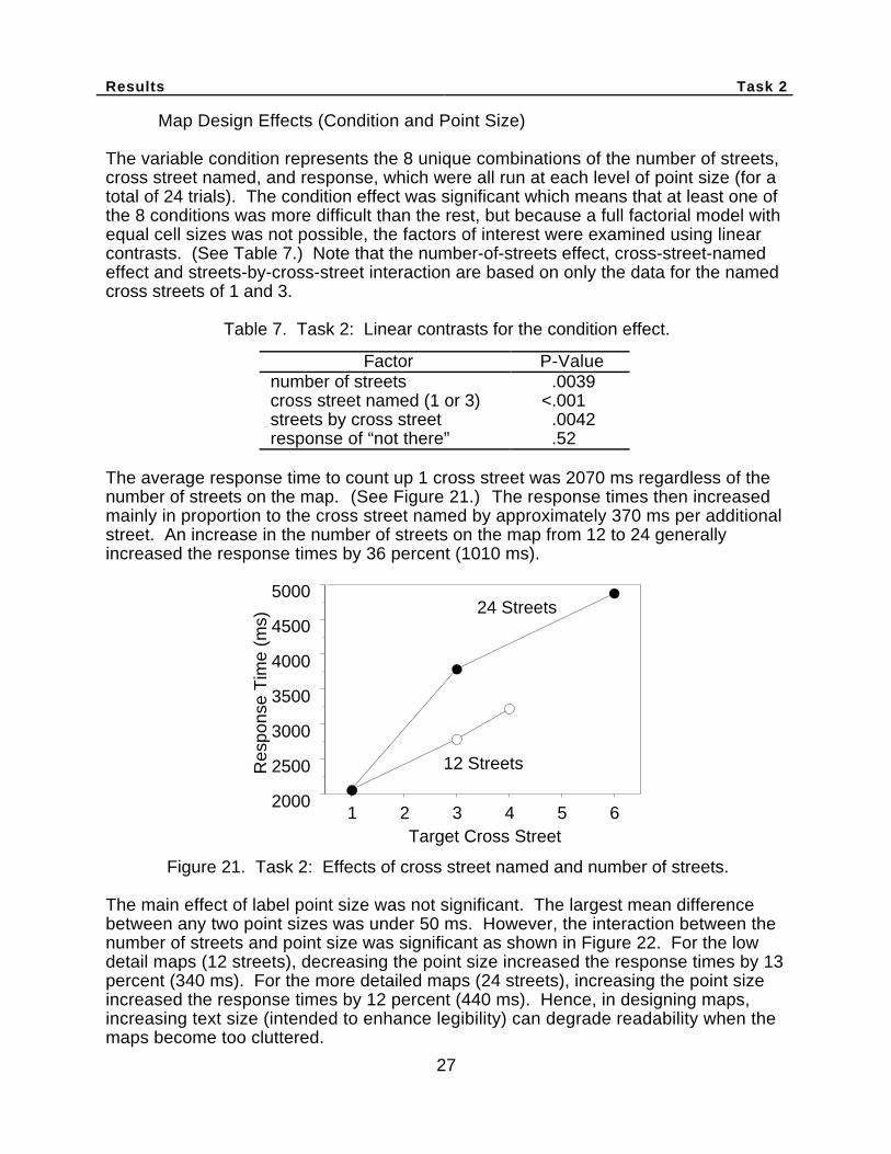
Map Design Effects (Condition and Point Size)
The variable condition represents the 8 unique combinations of the number of streets,cross street named, and response, which were all run at each level of point size (for atotal of 24 trials). The condition effect was significant which means that at least one ofthe 8 conditions was more difficult than the rest, but because a full factorial model withequal cell sizes was not possible, the factors of interest were examined using linearcontrasts. (See Table 7.) Note that the number-of-streets effect, cross-street-namedeffect and streets-by-cross-street interaction are based on only the data for the namedcross streets of 1 and 3.
Table 7. Task 2: Linear contrasts for the condition effect.
Factor P-Valuenumber of streets .0039cross street named (1 or 3) <.001streets by cross street .0042response of “not there” .52
The average response time to count up 1 cross street was 2070 ms regardless of thenumber of streets on the map. (See Figure 21.) The response times then increasedmainly in proportion to the cross street named by approximately 370 ms per additionalstreet. An increase in the number of streets on the map from 12 to 24 generallyincreased the response times by 36 percent (1010 ms).
1 2 3 4 5 62000
2500
3000
3500
4000
4500
5000
Res
pons
e T
ime
(ms)
Target Cross Street
24 Streets
12 Streets
Figure 21. Task 2: Effects of cross street named and number of streets.
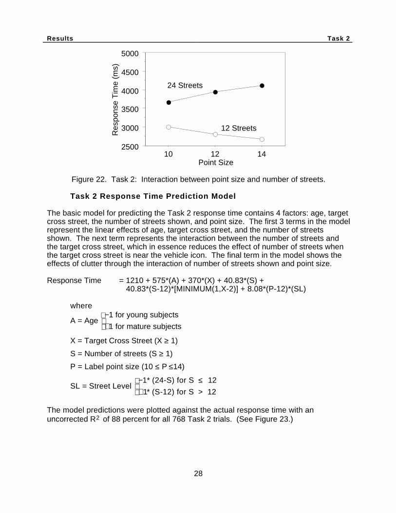
The main effect of label point size was not significant. The largest mean differencebetween any two point sizes was under 50 ms. However, the interaction between thenumber of streets and point size was significant as shown in Figure 22. For the lowdetail maps (12 streets), decreasing the point size increased the response times by 13percent (340 ms). For the more detailed maps (24 streets), increasing the point sizeincreased the response times by 12 percent (440 ms). Hence, in designing maps,increasing text size (intended to enhance legibility) can degrade readability when themaps become too cluttered.
Results Task 2
28
2500
3000
3500
4000
4500
5000
Res
pons
e T
ime
(ms)
10 12 14Point Size
24 Streets
12 Streets
Figure 22. Task 2: Interaction between point size and number of streets.
Task 2 Response Time Prediction Model
The basic model for predicting the Task 2 response time contains 4 factors: age, targetcross street, the number of streets shown, and point size. The first 3 terms in the modelrepresent the linear effects of age, target cross street, and the number of streetsshown. The next term represents the interaction between the number of streets andthe target cross street, which in essence reduces the effect of number of streets whenthe target cross street is near the vehicle icon. The final term in the model shows theeffects of clutter through the interaction of number of streets shown and point size.
Response Time = 1210 + 575*(A) + 370*(X) + 40.83*(S) +40.83*(S-12)*[MINIMUM(1,X-2)] + 8.08*(P-12)*(SL)
where
A = Age −1 for young subjects
+1 for mature subjects
X = Target Cross Street (X ≥ 1)
S = Number of streets (S ≥ 1)
P = Label point size (10 ≤ P ≤14)
SL = Street Level −1∗ (24-S) for S ≤ 12
+1∗ (S-12) for S > 12
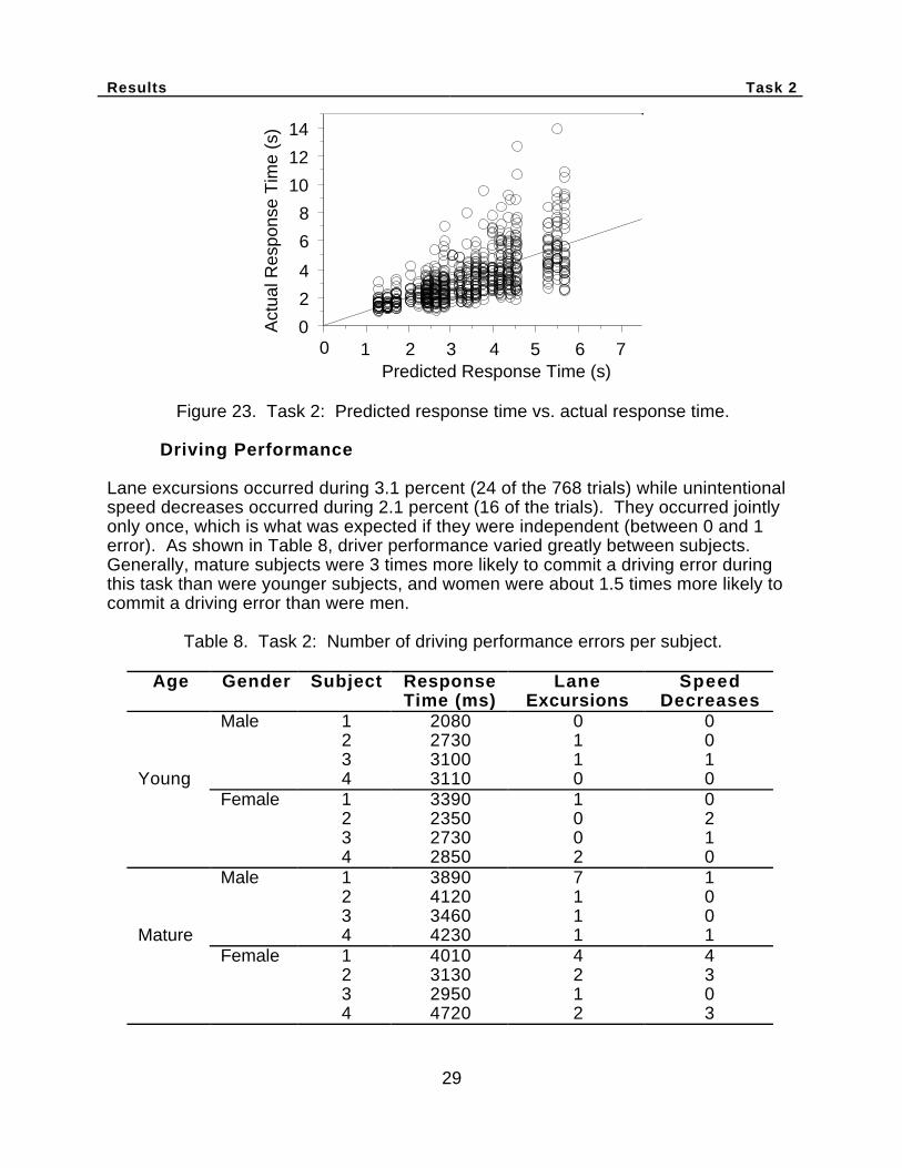
The model predictions were plotted against the actual response time with anuncorrected R2 of 88 percent for all 768 Task 2 trials. (See Figure 23.)
Results Task 2
29
0
2
4
6
8
10
12
14
Act
ual R
espo
nse
Tim
e (s
)
0 2 4 6Predicted Response Time (s)
3 5 71
Figure 23. Task 2: Predicted response time vs. actual response time.
Driving Performance
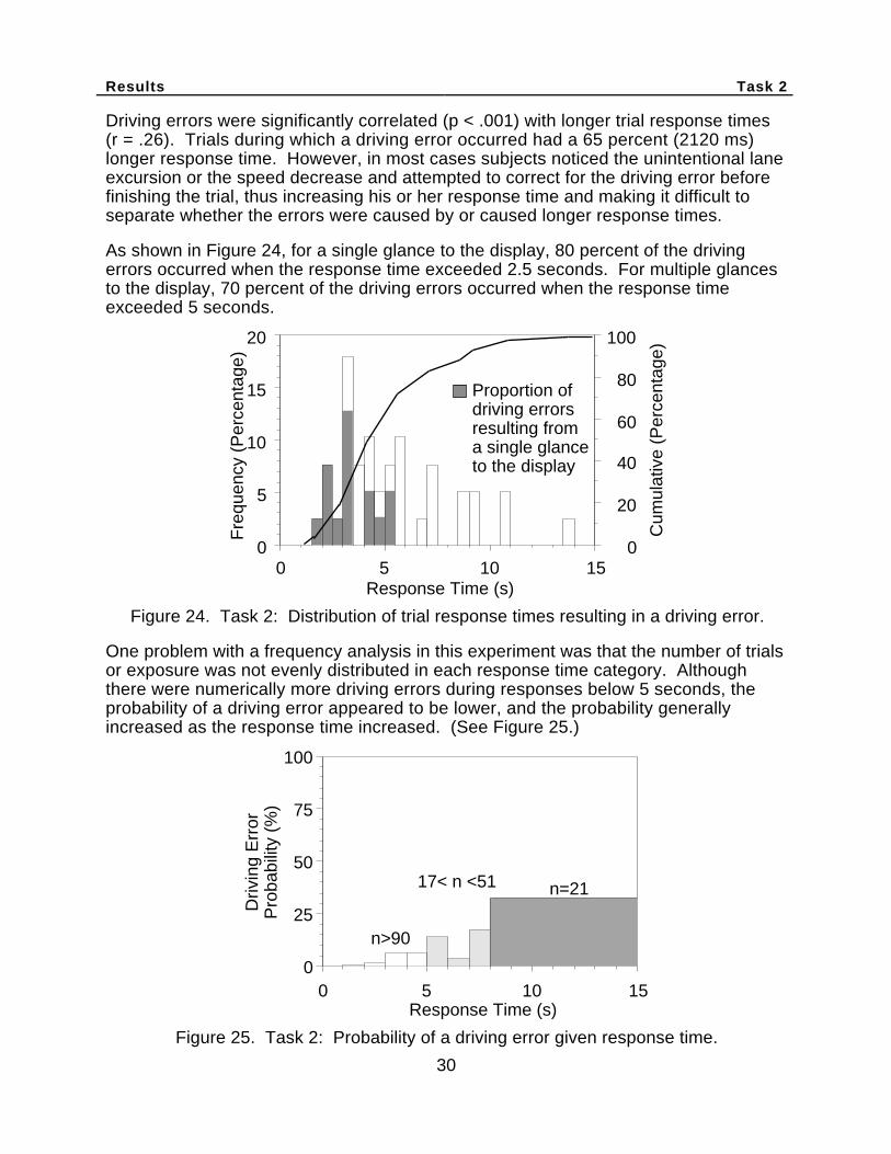
Lane excursions occurred during 3.1 percent (24 of the 768 trials) while unintentionalspeed decreases occurred during 2.1 percent (16 of the trials). They occurred jointlyonly once, which is what was expected if they were independent (between 0 and 1error). As shown in Table 8, driver performance varied greatly between subjects.Generally, mature subjects were 3 times more likely to commit a driving error duringthis task than were younger subjects, and women were about 1.5 times more likely tocommit a driving error than were men.
Table 8. Task 2: Number of driving performance errors per subject.
Age Gender Subject ResponseTime (ms)
LaneExcursions
SpeedDecreases
Male 1 2080 0 02 2730 1 03 3100 1 1
Young 4 3110 0 0Female 1 3390 1 0
2 2350 0 23 2730 0 14 2850 2 0
Male 1 3890 7 12 4120 1 03 3460 1 0
Mature 4 4230 1 1Female 1 4010 4 4
2 3130 2 33 2950 1 04 4720 2 3
Results Task 2
30
Driving errors were significantly correlated (p < .001) with longer trial response times(r = .26). Trials during which a driving error occurred had a 65 percent (2120 ms)longer response time. However, in most cases subjects noticed the unintentional laneexcursion or the speed decrease and attempted to correct for the driving error beforefinishing the trial, thus increasing his or her response time and making it difficult toseparate whether the errors were caused by or caused longer response times.
As shown in Figure 24, for a single glance to the display, 80 percent of the drivingerrors occurred when the response time exceeded 2.5 seconds. For multiple glancesto the display, 70 percent of the driving errors occurred when the response timeexceeded 5 seconds.
0
5
10
15
20
Fre
quen
cy (
Per
cent
age)
0
20
40
60
80
100
0 5 10 15Response Time (s)
Cum
ulat
ive
(Per
cent
age)
Proportion ofdriving errorsresulting froma single glanceto the display
Figure 24. Task 2: Distribution of trial response times resulting in a driving error.
One problem with a frequency analysis in this experiment was that the number of trialsor exposure was not evenly distributed in each response time category. Althoughthere were numerically more driving errors during responses below 5 seconds, theprobability of a driving error appeared to be lower, and the probability generallyincreased as the response time increased. (See Figure 25.)
Response Time (s)
0
25
50
75
100
Driv
ing
Err
orP
roba
bilit
y (%
)
n=2117< n <51
n>90
0 5 10 15
Figure 25. Task 2: Probability of a driving error given response time.
Results Task 2
31
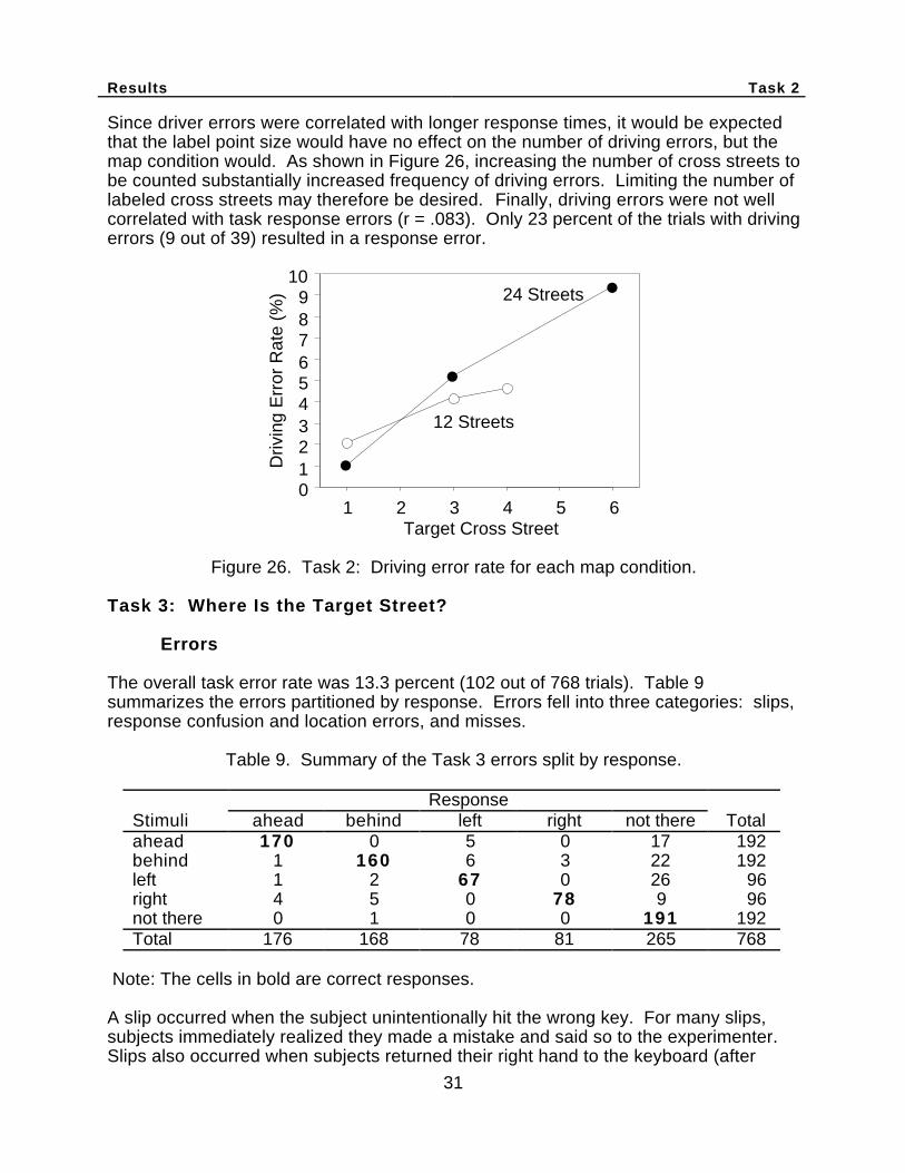
Since driver errors were correlated with longer response times, it would be expectedthat the label point size would have no effect on the number of driving errors, but themap condition would. As shown in Figure 26, increasing the number of cross streets tobe counted substantially increased frequency of driving errors. Limiting the number oflabeled cross streets may therefore be desired. Finally, driving errors were not wellcorrelated with task response errors (r = .083). Only 23 percent of the trials with drivingerrors (9 out of 39) resulted in a response error.
Driv
ing
Err
or R
ate
(%)
1 2 3 4 5 6Target Cross Street
24 Streets
12 Streets
0123456789
10
Figure 26. Task 2: Driving error rate for each map condition.
Task 3: Where Is the Target Street?
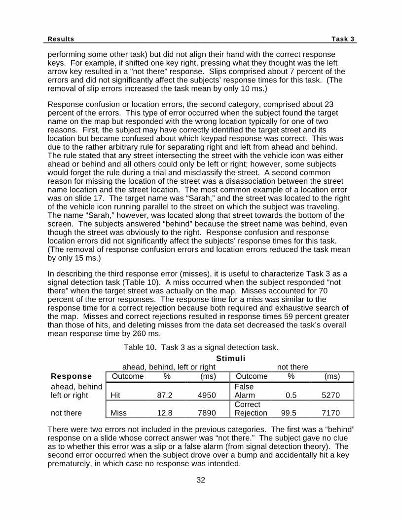
Errors
The overall task error rate was 13.3 percent (102 out of 768 trials). Table 9summarizes the errors partitioned by response. Errors fell into three categories: slips,response confusion and location errors, and misses.
Table 9. Summary of the Task 3 errors split by response.
ResponseStimuli ahead behind left right not there Totalahead 170 0 5 0 17 192behind 1 160 6 3 22 192left 1 2 67 0 26 96right 4 5 0 78 9 96not there 0 1 0 0 191 192Total 176 168 78 81 265 768
Note: The cells in bold are correct responses.
A slip occurred when the subject unintentionally hit the wrong key. For many slips,subjects immediately realized they made a mistake and said so to the experimenter.Slips also occurred when subjects returned their right hand to the keyboard (after
Results Task 3
32
performing some other task) but did not align their hand with the correct responsekeys. For example, if shifted one key right, pressing what they thought was the leftarrow key resulted in a "not there" response. Slips comprised about 7 percent of theerrors and did not significantly affect the subjects’ response times for this task. (Theremoval of slip errors increased the task mean by only 10 ms.)
Response confusion or location errors, the second category, comprised about 23percent of the errors. This type of error occurred when the subject found the targetname on the map but responded with the wrong location typically for one of tworeasons. First, the subject may have correctly identified the target street and itslocation but became confused about which keypad response was correct. This wasdue to the rather arbitrary rule for separating right and left from ahead and behind.The rule stated that any street intersecting the street with the vehicle icon was eitherahead or behind and all others could only be left or right; however, some subjectswould forget the rule during a trial and misclassify the street. A second commonreason for missing the location of the street was a disassociation between the streetname location and the street location. The most common example of a location errorwas on slide 17. The target name was “Sarah,” and the street was located to the rightof the vehicle icon running parallel to the street on which the subject was traveling.The name “Sarah,” however, was located along that street towards the bottom of thescreen. The subjects answered “behind” because the street name was behind, eventhough the street was obviously to the right. Response confusion and responselocation errors did not significantly affect the subjects’ response times for this task.(The removal of response confusion errors and location errors reduced the task meanby only 15 ms.)
In describing the third response error (misses), it is useful to characterize Task 3 as asignal detection task (Table 10). A miss occurred when the subject responded “notthere” when the target street was actually on the map. Misses accounted for 70percent of the error responses. The response time for a miss was similar to theresponse time for a correct rejection because both required and exhaustive search ofthe map. Misses and correct rejections resulted in response times 59 percent greaterthan those of hits, and deleting misses from the data set decreased the task’s overallmean response time by 260 ms.
Table 10. Task 3 as a signal detection task.Stimuli
ahead, behind, left or right not thereResponse Outcome % (ms) Outcome % (ms)ahead, behindleft or right Hit 87.2 4950
FalseAlarm 0.5 5270
not there Miss 12.8 7890CorrectRejection 99.5 7170
There were two errors not included in the previous categories. The first was a “behind”response on a slide whose correct answer was “not there.” The subject gave no clueas to whether this error was a slip or a false alarm (from signal detection theory). Thesecond error occurred when the subject drove over a bump and accidentally hit a keyprematurely, in which case no response was intended.
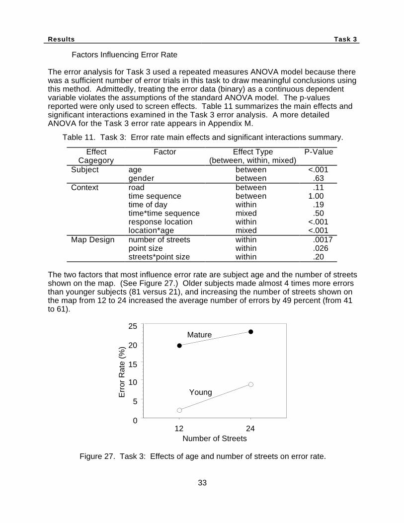
Results Task 3
33
Factors Influencing Error Rate
The error analysis for Task 3 used a repeated measures ANOVA model because therewas a sufficient number of error trials in this task to draw meaningful conclusions usingthis method. Admittedly, treating the error data (binary) as a continuous dependentvariable violates the assumptions of the standard ANOVA model. The p-valuesreported were only used to screen effects. Table 11 summarizes the main effects andsignificant interactions examined in the Task 3 error analysis. A more detailedANOVA for the Task 3 error rate appears in Appendix M.
Table 11. Task 3: Error rate main effects and significant interactions summary.
EffectCagegory
Factor Effect Type(between, within, mixed)
P-Value
Subject age between <.001gender between .63
Context road between .11time sequence between 1.00time of day within .19time*time sequence mixed .50response location within <.001location*age mixed <.001
Map Design number of streets within .0017point size within .026streets*point size within .20
The two factors that most influence error rate are subject age and the number of streetsshown on the map. (See Figure 27.) Older subjects made almost 4 times more errorsthan younger subjects (81 versus 21), and increasing the number of streets shown onthe map from 12 to 24 increased the average number of errors by 49 percent (from 41to 61).
Mature
Err
or R
ate
(%)
12 24Number of Streets
Young
0
5
10
15
20
25
Figure 27. Task 3: Effects of age and number of streets on error rate.
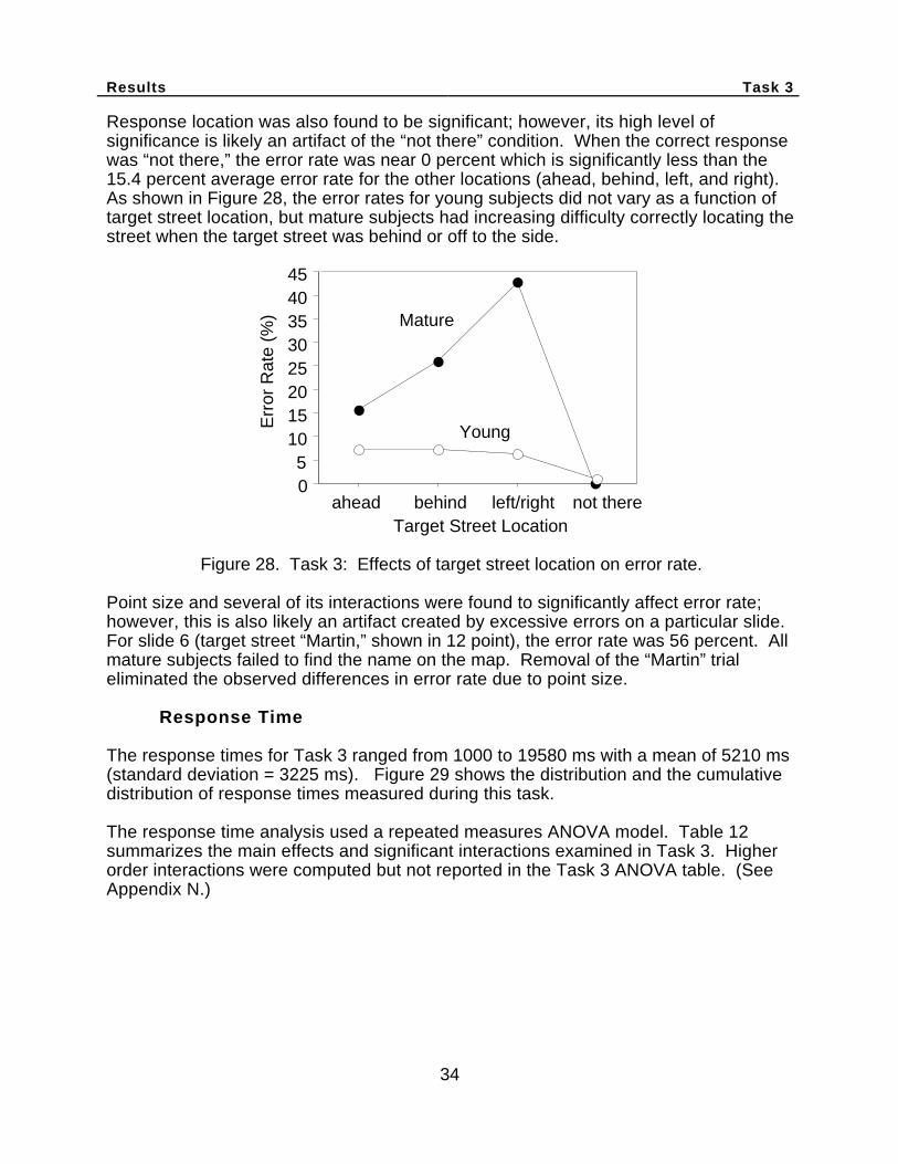
Results Task 3
34
Response location was also found to be significant; however, its high level ofsignificance is likely an artifact of the “not there” condition. When the correct responsewas “not there,” the error rate was near 0 percent which is significantly less than the15.4 percent average error rate for the other locations (ahead, behind, left, and right).As shown in Figure 28, the error rates for young subjects did not vary as a function oftarget street location, but mature subjects had increasing difficulty correctly locating thestreet when the target street was behind or off to the side.
05
1015202530354045
Err
or R
ate
(%)
ahead behind left/right not thereTarget Street Location
Mature
Young
Figure 28. Task 3: Effects of target street location on error rate.
Point size and several of its interactions were found to significantly affect error rate;however, this is also likely an artifact created by excessive errors on a particular slide.For slide 6 (target street “Martin,” shown in 12 point), the error rate was 56 percent. Allmature subjects failed to find the name on the map. Removal of the “Martin” trialeliminated the observed differences in error rate due to point size.
Response Time
The response times for Task 3 ranged from 1000 to 19580 ms with a mean of 5210 ms(standard deviation = 3225 ms). Figure 29 shows the distribution and the cumulativedistribution of response times measured during this task.
The response time analysis used a repeated measures ANOVA model. Table 12summarizes the main effects and significant interactions examined in Task 3. Higherorder interactions were computed but not reported in the Task 3 ANOVA table. (SeeAppendix N.)

Results Task 3
35
0
1
2
3
4
5
6
Fre
quen
cy (
Per
cent
age)
0 5 10 15 20Response Time (s)
10
20
30
40
50
60
70
80
90
100
Cum
ulat
ive
(Per
cent
age)
Figure 29. Task 3: Distribution of response times.
Table 12. Task 3: Response time main effects and significant interactions summary.
EffectCategory
Factor Effect Type(between, within,
mixed)
P-Value
Subject age between .0018gender between .78age*gender between .31
Context road between .063time sequence between .60time of day within .068time*timesequence
mixed .72
response location within <.001Map Design number of streets within <.001
streets*age mixed .035streets*location within .0033point size within .16
Subject Effects (Age and Gender)
Age was the only statistically significant subject effect. The difference between maturesubjects (mean 6710 ms) and young subjects (mean 3710 ms) was 3000 ms (anincrease of 81 percent). Gender was not significant and neither was an age-by-gender interaction with a mean absolute difference between men and women of only120 ms. Variability increased with the subject age (2030 ms for young subjects, 3490ms for mature subjects). Figure 30 shows the effects of age and gender.
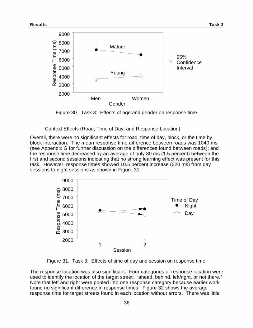
Results Task 3
36
Mature
2000
3000
4000
5000
6000
7000
8000
9000
Res
pons
e T
ime
(ms)
Men WomenGender
Young
95%ConfidenceInterval
Figure 30. Task 3: Effects of age and gender on response time.
Context Effects (Road, Time of Day, and Response Location)
Overall, there were no significant effects for road, time of day, block, or the time byblock interaction. The mean response time difference between roads was 1040 ms(see Appendix G for further discussion on the differences found between roads); andthe response time decreased by an average of only 80 ms (1.5 percent) between thefirst and second sessions indicating that no strong learning effect was present for thistask. However, response times showed 10.5 percent increase (520 ms) from daysessions to night sessions as shown in Figure 31.
Night
2000
3000
4000
5000
6000
7000
8000
9000
Res
pons
e T
ime
(ms)
1 2Session
Day
Time of Day
Figure 31. Task 3: Effects of time of day and session on response time.
The response location was also significant. Four categories of response location wereused to identify the location of the target street: “ahead, behind, left/right, or not there.”Note that left and right were pooled into one response category because earlier workfound no significant difference in response times. Figure 32 shows the averageresponse time for target streets found in each location without errors. There was little
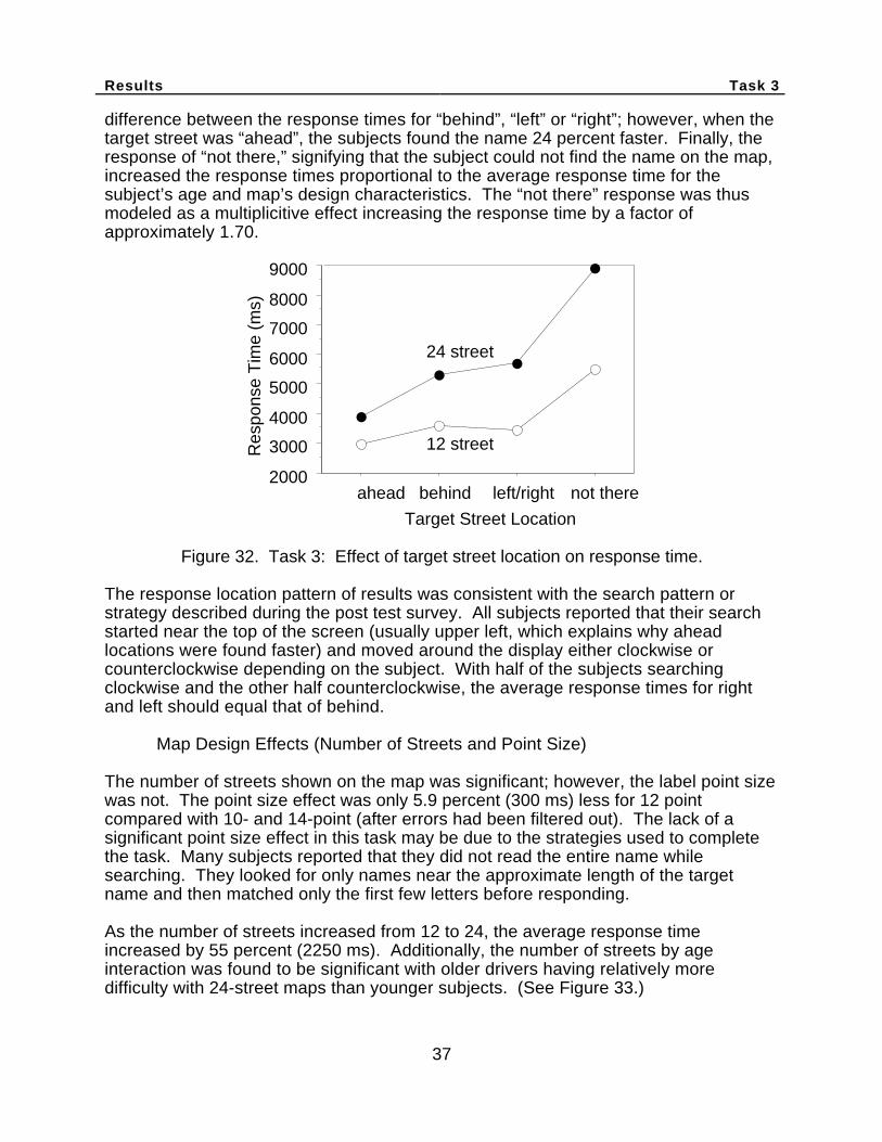
Results Task 3
37
difference between the response times for “behind”, “left” or “right”; however, when thetarget street was “ahead”, the subjects found the name 24 percent faster. Finally, theresponse of “not there,” signifying that the subject could not find the name on the map,increased the response times proportional to the average response time for thesubject’s age and map’s design characteristics. The “not there” response was thusmodeled as a multiplicitive effect increasing the response time by a factor ofapproximately 1.70.
2000
3000
4000
5000
6000
7000
8000
9000R
espo
nse
Tim
e (m
s)
ahead left/right not there
Target Street Location
behind
12 street
24 street
Figure 32. Task 3: Effect of target street location on response time.
The response location pattern of results was consistent with the search pattern orstrategy described during the post test survey. All subjects reported that their searchstarted near the top of the screen (usually upper left, which explains why aheadlocations were found faster) and moved around the display either clockwise orcounterclockwise depending on the subject. With half of the subjects searchingclockwise and the other half counterclockwise, the average response times for rightand left should equal that of behind.
Map Design Effects (Number of Streets and Point Size)
The number of streets shown on the map was significant; however, the label point sizewas not. The point size effect was only 5.9 percent (300 ms) less for 12 pointcompared with 10- and 14-point (after errors had been filtered out). The lack of asignificant point size effect in this task may be due to the strategies used to completethe task. Many subjects reported that they did not read the entire name whilesearching. They looked for only names near the approximate length of the targetname and then matched only the first few letters before responding.
As the number of streets increased from 12 to 24, the average response timeincreased by 55 percent (2250 ms). Additionally, the number of streets by ageinteraction was found to be significant with older drivers having relatively moredifficulty with 24-street maps than younger subjects. (See Figure 33.)
Results Task 3
38
2000
3000
4000
5000
6000
7000
8000
9000
12 24Number of Streets
Res
pons
e T
ime
(ms) Mature
Young
Figure 33. Task 3: Effects of age and number of streets on response time.
Task 3 Response Time Prediction Model
The basic model for predicting the Task 3 response time contains 5 factors: age, timeof day, the number of streets shown, the target location, and the search result. The first3 terms in the model represent the linear effects of age, time of day, and the number ofstreets shown. The next term represents the interaction between the number of streetsshown and the subject’s age. The final 2 terms in the model show the effects of thetarget street location and the search result.
Response Time = [1630 + 1235*(A) + 380*(T) + 136*(S) + 27*(A)*(SL) + 475*(L)]*(SR)
where
A = Age −1 for young subjects
+1 for mature subjects
T = Time of day −1 for day
+1 for night
S = Number of streets (S ≥ 1)
SL = Street Level −1∗ (24-S) for S ≤ 12
+1∗ (S-12) for S > 12
L = Target Location −1 for ahead 0 for not there+1 for behind, left or right
SR = Search Result 1 if target is found
1.70 if target is not found
The model predictions were plotted against the actual response time in Figure 34 withan uncorrected R2 of 87 percent for all 768 Task 3 trials.
Results Task 3
39
0
5
10
15
20
25
Act
ual R
espo
nse
Tim
e (s
)
0 5 10Predicted Response Time (s)
1 2 3 4 6 7 8 9 11 12
Figure 34. Task 3: Predicted response time vs. actual response time.
Driving Performance
Lane excursions occurred during 5 percent (41) of the trials while unintentional speeddecreases occurred during 6 percent (46) of the trials. They occurred together on onlysix trials (versus only two if they were truly independent), suggesting little or nodependency. As in Task 2, driving performance varied greatly between subjects.(See Table 13.) Generally, mature subjects committed twice as many driving errors inthis task as younger subjects, and women committed 1.5 times as many driving errorsas did men.
Table 13. Task 3: Number of driving performance errors per subject.
Age Gender Subject ResponseTime (ms)
LaneExcursions
SpeedDecreases
Male 1 3420 0 02 3390 0 03 4270 0 2
Young 4 3060 0 0Female 1 5130 3 2
2 3500 3 13 3780 0 24 3140 1 0
Male 1 7310 3 92 7320 0 93 5450 0 2
Mature 4 7950 9 10Female 1 8470 8 14
2 7320 1 43 4800 6 04 5090 6 0
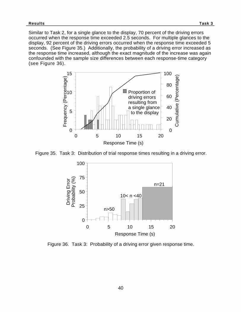
Results Task 3
40
Similar to Task 2, for a single glance to the display, 70 percent of the driving errorsoccurred when the response time exceeded 2.5 seconds. For multiple glances to thedisplay, 92 percent of the driving errors occurred when the response time exceeded 5seconds. (See Figure 35.) Additionally, the probability of a driving error increased asthe response time increased, although the exact magnitude of the increase was againconfounded with the sample size differences between each response-time category(see Figure 36).
0
5
10
15
Fre
quen
cy (
Per
cent
age)
0 5 10 15 20
Response Time (s)
0
20
40
60
80
100
Cum
ulat
ive
(Per
cent
age)
Proportion ofdriving errorsresulting froma single glance to the display
Figure 35. Task 3: Distribution of trial response times resulting in a driving error.
0 5 10 15 20
Response Time (s)
0
25
50
75
100
Driv
ing
Err
orP
roba
bilit
y (%
)
n=21
10< n <40
n>50
Figure 36. Task 3: Probability of a driving error given response time.
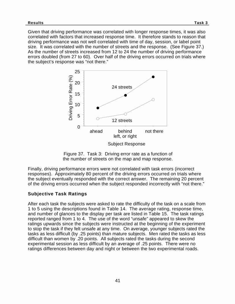
Results Task 3
41
Given that driving performance was correlated with longer response times, it was alsocorrelated with factors that increased response time. It therefore stands to reason thatdriving performance was not well correlated with time of day, session, or label pointsize. It was correlated with the number of streets and the response. (See Figure 37.)As the number of streets increased from 12 to 24 the number of driving performanceerrors doubled (from 27 to 60). Over half of the driving errors occurred on trials wherethe subject’s response was “not there.”
0
5
10
15
20
25D
rivin
g E
rror
Rat
e (%
)
ahead behindleft, or right
not there
Subject Response
12 streets
24 streets
Figure 37. Task 3: Driving error rate as a function ofthe number of streets on the map and map response.
Finally, driving performance errors were not correlated with task errors (incorrectresponses). Approximately 80 percent of the driving errors occurred on trials wherethe subject eventually responded with the correct answer. The remaining 20 percentof the driving errors occurred when the subject responded incorrectly with “not there.”
Subjective Task Ratings
After each task the subjects were asked to rate the difficulty of the task on a scale from1 to 5 using the descriptions found in Table 14. The average rating, response time,and number of glances to the display per task are listed in Table 15. The task ratingsreported ranged from 1 to 4. The use of the word “unsafe” appeared to skew theratings upwards since the subjects were instructed at the beginning of the experimentto stop the task if they felt unsafe at any time. On average, younger subjects rated thetasks as less difficult (by .25 points) than mature subjects. Men rated the tasks as lessdifficult than women by .20 points. All subjects rated the tasks during the secondexperimental session as less difficult by an average of .25 points. There were noratings differences between day and night or between the two experimental roads.
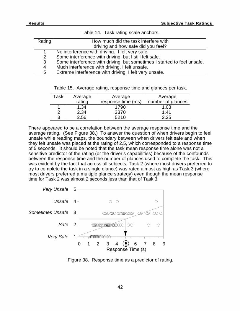
Results Subjective Task Ratings
42
Table 14. Task rating scale anchors.
Rating How much did the task interfere withdriving and how safe did you feel?
1 No interference with driving. I felt very safe.2 Some interference with driving, but I still felt safe.3 Some interference with driving, but sometimes I started to feel unsafe.4 Much interference with driving, I felt unsafe.5 Extreme interference with driving, I felt very unsafe.
Table 15. Average rating, response time and glances per task.
Task Averagerating
Averageresponse time (ms)
Averagenumber of glances
1 1.34 1790 1.032 2.34 3370 1.413 2.56 5210 2.25
There appeared to be a correlation between the average response time and theaverage rating. (See Figure 38.) To answer the question of when drivers begin to feelunsafe while reading maps, the boundary between when drivers felt safe and whenthey felt unsafe was placed at the rating of 2.5, which corresponded to a response timeof 5 seconds. It should be noted that the task mean response time alone was not asensitive predictor of the rating (or the driver’s capabilities) because of the confoundsbetween the response time and the number of glances used to complete the task. Thiswas evident by the fact that across all subjects, Task 2 (where most drivers preferred totry to complete the task in a single glance) was rated almost as high as Task 3 (wheremost drivers preferred a multiple glance strategy) even though the mean responsetime for Task 2 was almost 2 seconds less than that of Task 3.
0 2 4 6 8Response Time (s)31 75 9
Very Safe 1
Very Unsafe 5
Safe 2
Sometimes Unsafe 3
Unsafe 4
Figure 38. Response time as a predictor of rating.
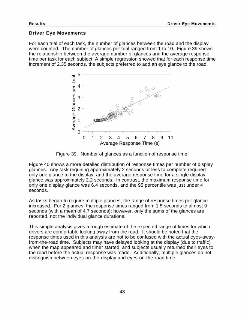
Results Driver Eye Movements
43
Driver Eye Movements
For each trial of each task, the number of glances between the road and the displaywere counted. The number of glances per trial ranged from 1 to 10. Figure 39 showsthe relationship between the average number of glances and the average responsetime per task for each subject. A simple regression showed that for each response timeincrement of 2.35 seconds, the subjects preferred to add an eye glance to the road.
0
1
2
3
4
5A
vera
ge G
lanc
es p
er T
rial
0 2 4 6 8 10Average Response Time (s)
31 75 9
Figure 39. Number of glances as a function of response time.
Figure 40 shows a more detailed distribution of response times per number of displayglances. Any task requiring approximately 2 seconds or less to complete requiredonly one glance to the display, and the average response time for a single displayglance was approximately 2.2 seconds. In contrast, the maximum response time foronly one display glance was 6.4 seconds, and the 95 percentile was just under 4seconds.
As tasks began to require multiple glances, the range of response times per glanceincreased. For 2 glances, the response times ranged from 1.5 seconds to almost 9seconds (with a mean of 4.7 seconds); however, only the sums of the glances arereported, not the individual glance durations.
This simple analysis gives a rough estimate of the expected range of times for whichdrivers are comfortable looking away from the road. It should be noted that theresponse times used in this analysis are not to be confused with the actual eyes-away-from-the-road time. Subjects may have delayed looking at the display (due to traffic)when the map appeared and timer started, and subjects usually returned their eyes tothe road before the actual response was made. Additionally, multiple glances do notdistinguish between eyes-on-the-display and eyes-on-the-road time.
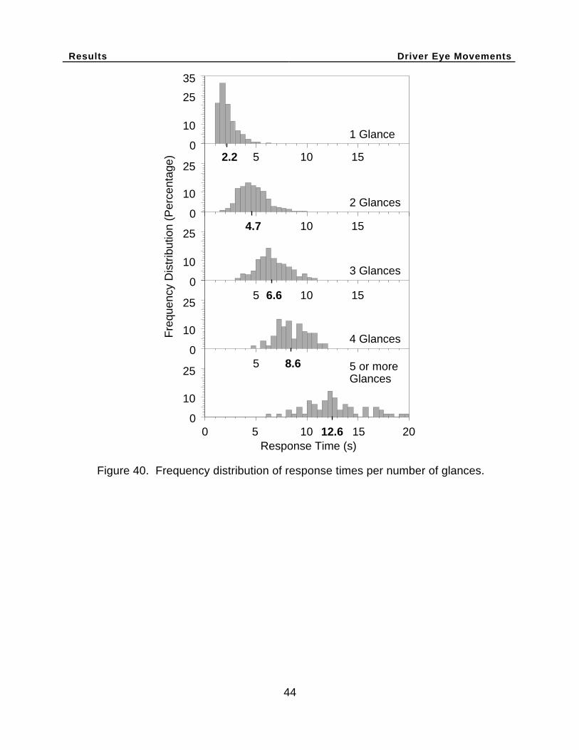
Results Driver Eye Movements
44
0
10
25
35
0
10
25
0
10
2510 15
5 10 15
0
10
25
0
10
25
0 5 10 15 20Response Time (s)
1 Glance
2 Glances
3 Glances
4 Glances
5 or moreGlances
Fre
quen
cy D
istr
ibut
ion
(Per
cent
age)
5 10 15
5
2.2
4.7
6.6
8.6
12.6
Figure 40. Frequency distribution of response times per number of glances.
Conclusions
45
CONCLUSIONS
How long does it take on average to read an electronic map?
Three tasks ranging in difficulty were examined in this experiment. Task 1 (What streetare you on?) was relatively easy. The response times for this task ranged from 1 to 2.5seconds and in most cases required only a single glance to the display. Task 2 (Whatis the nth cross street?) required a more difficult structured search of the map.Response times for this task increased as the number of the target cross streetincreased. The average response times ranged from 1.6 to 5.2 seconds requiring 1.5glances (on average) to the display. Task 3 (Where is the target street?) required aneven more difficult unstructured search of the map. The response time increased inproportion to the number of items to be searched with typical response times rangingfrom 2 to 8.4 seconds and requiring, on average, 2.25 glances to the display.
When do the drivers feel that map reading is unsafe while driving?
During expressway driving, the natural tendency of drivers was to limit their visualinteraction with the system to under 3 seconds per glance. According to the data ondriving errors for a single glance to the display, the number of lane excursions andlosses of speed would be reduced by 80 percent if the task required no more than 2seconds of visual attention to complete (not including transition times).
Although the driver preference data collected was biased by the anchors in the ratingscale, the driver preferences should also be considered. Since the rating scaleanchored the drivers’ impressions of “safe” at 2 and “unsafe” at 3, a rating of 2.5 couldbe considered a design threshold not to be exceeded. A rating of 2.5 in thisexperiment corresponded to an average response time of about 5 seconds,suggesting that drivers become uncomfortable when their interactions with the systemrequire more than two glances (since drivers limited each glance to under 3 seconds).The driving-error data also supports this conclusion since 86 percent of the multiple-glance driving errors occurred when the response time was greater than 5 seconds.
Given the drivers’ tendencies and preferences as described above, two map designcriteria can be recommended that would reduce the overall number of driving errors by85 percent. Tasks requiring the driver’s visual attention while the vehicle is in motionshould be designed such that they can be completed using, first, display glances of nomore than 2 seconds and, second, no more than a total of 2 display glances.
How did age and gender affect the map reading time?
The only subject effect consistently significant across all tasks was the driver’s age.The response time differences between younger and mature drivers increased as thetask difficulty increased. For a relatively easy task such as Task 1, the reading timeswere 40 percent greater for older subjects, and for a more difficult search task, Task 3,the response times for older subjects were up to 80 percent longer. The age effectalso increased within the task as the within task difficulty increased. Additionally,mature subjects were more sensitive to many of the variables tested (point size in Task1 and target street location in Task 3) than were younger subjects.
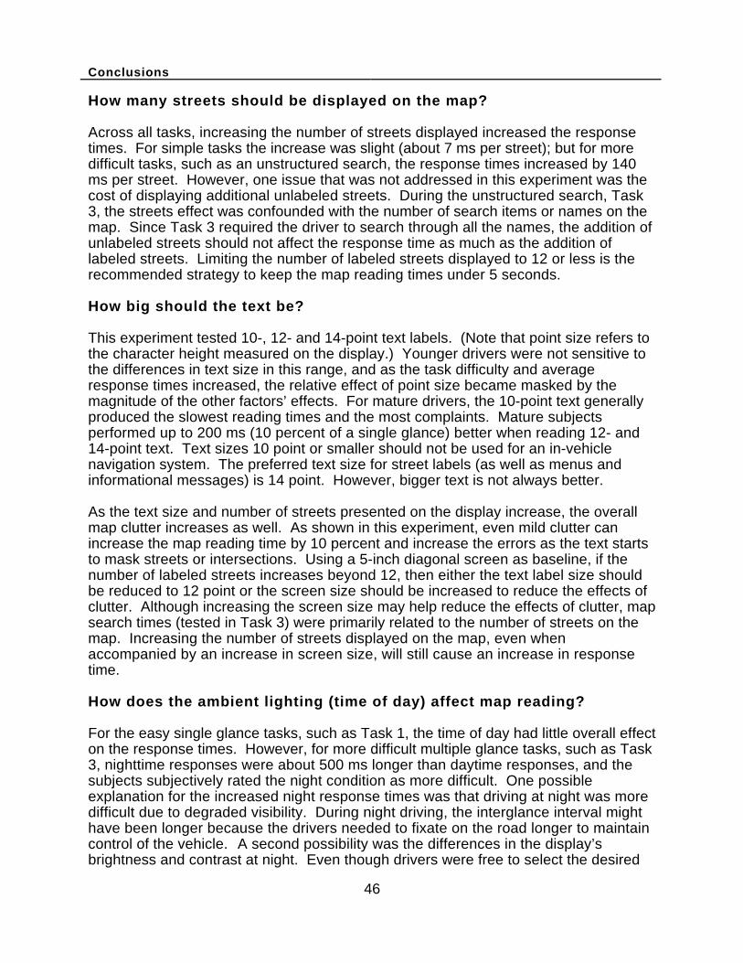
Conclusions
46
How many streets should be displayed on the map?
Across all tasks, increasing the number of streets displayed increased the responsetimes. For simple tasks the increase was slight (about 7 ms per street); but for moredifficult tasks, such as an unstructured search, the response times increased by 140ms per street. However, one issue that was not addressed in this experiment was thecost of displaying additional unlabeled streets. During the unstructured search, Task3, the streets effect was confounded with the number of search items or names on themap. Since Task 3 required the driver to search through all the names, the addition ofunlabeled streets should not affect the response time as much as the addition oflabeled streets. Limiting the number of labeled streets displayed to 12 or less is therecommended strategy to keep the map reading times under 5 seconds.
How big should the text be?
This experiment tested 10-, 12- and 14-point text labels. (Note that point size refers tothe character height measured on the display.) Younger drivers were not sensitive tothe differences in text size in this range, and as the task difficulty and averageresponse times increased, the relative effect of point size became masked by themagnitude of the other factors’ effects. For mature drivers, the 10-point text generallyproduced the slowest reading times and the most complaints. Mature subjectsperformed up to 200 ms (10 percent of a single glance) better when reading 12- and14-point text. Text sizes 10 point or smaller should not be used for an in-vehiclenavigation system. The preferred text size for street labels (as well as menus andinformational messages) is 14 point. However, bigger text is not always better.
As the text size and number of streets presented on the display increase, the overallmap clutter increases as well. As shown in this experiment, even mild clutter canincrease the map reading time by 10 percent and increase the errors as the text startsto mask streets or intersections. Using a 5-inch diagonal screen as baseline, if thenumber of labeled streets increases beyond 12, then either the text label size shouldbe reduced to 12 point or the screen size should be increased to reduce the effects ofclutter. Although increasing the screen size may help reduce the effects of clutter, mapsearch times (tested in Task 3) were primarily related to the number of streets on themap. Increasing the number of streets displayed on the map, even whenaccompanied by an increase in screen size, will still cause an increase in responsetime.
How does the ambient lighting (time of day) affect map reading?
For the easy single glance tasks, such as Task 1, the time of day had little overall effecton the response times. However, for more difficult multiple glance tasks, such as Task3, nighttime responses were about 500 ms longer than daytime responses, and thesubjects subjectively rated the night condition as more difficult. One possibleexplanation for the increased night response times was that driving at night was moredifficult due to degraded visibility. During night driving, the interglance interval mighthave been longer because the drivers needed to fixate on the road longer to maintaincontrol of the vehicle. A second possibility was the differences in the display’sbrightness and contrast at night. Even though drivers were free to select the desired

Conclusions
47
brightness and contrast for the in-vehicle display at night, drivers may not haveselected an optimal setting.
Two interesting lessons were learned from the night sessions. First, although time ofday had little effect on the response times for simple tasks, learning the tasksappeared more difficult at night. In all tasks, the learning effect between experimentalsessions was amplified for those driving the night session first. Second, the issues ofcolor selection and brightness are important at night. The pilot tests used black text ona white background to maximize contrast, but all drivers agreed that this combinationwas far too bright and distracting for night driving. For the actual experiment, the whitebackground was replaced with a grey (decreasing the brightness but reducing thecontrast); however, user preferences on this issue varied greatly with some requestingmore luminance and some requesting much less. Clearly, the issues of color,luminance, and contrast preferences need to be addressed in further research.
How can response time be predicted given the map design?
The response-time regression equations for the three tasks are summarized inTable 16. These equations can be used to predict the driver’s response time giventhe task and the map-design characteristics.
Table 16. Summary of response time prediction equations.
ResponseTime (ms)
Predictive Equation
Task 1 = 6710 + 325*(A) + 6.67*(S) + 33.75*(P)2 - 832.50*(P) + 9.58*(C)
Task 2 = 1210 + 575*(A) + 370*(X) + 40.83*(S) + 8.08*(P-12)*(SL) +40.83*(S-12)*[MINIMUM(1,X-2)]
Task 3 = [1630 + 1235*(A) + 380*(T) + 136*(S) + 27*(A)*(SL) + 475*(L)]*(SR)
Factor Definitions
A = Age −1 for young subjects
+1 for mature subjects
T = Time of day −1 for day
+1 for night
S = Number of streets (S ≥ 1) P = Label point size (10 ≤ P ≤14)
X = Target Cross Street (X ≥ 1) L = Target
Location −1 for ahead 0 for not there+1 for behind, left or right
SL = StreetLevel
−1∗ (24-S) for S ≤ 12
+1∗ (S-12) for S > 12
SR = SearchResult
1 if target is found
1.70 if target is not found
C = Clutter 0 for point size ≤ 12
(P − 12)(S-12.52) for point size > 12

48
Simulator Validation Method
49
SIMULATOR VALIDATION
Validation Method
A second goal of this experiment was to validate the use of a driving simulator to studysecondary response-time tasks. To allow for a comparison between the simulator andthe on-the-road experiment, the two experiments contained a common subset of map-design conditions. Both the simulated and the real roads used were relatively easy todrive with no sharp curves and low traffic volumes, but no effort was made to exactlymatch their difficulty. The comparison looked at two tasks, Task 1 and Task 3. Task 1represents a relatively easy task with response times ranging from 1 to 3 seconds andin most cases requiring only a single glance from the road to the display. Task 3, incontrast, represents a more difficult task with response times ranging from 1 to 20seconds and in most cases requiring multiple glances between the road and thedisplay. Due to the complexity of analysis and the low sample size (few trials hadoverlapping conditions between experiments), Task 2 was not validated. Thesimulator experiment used 20 subjects equally blocked for age and gender, while theon-the-road experiment used only 16 subjects (again equally blocked for age andgender). Each subject only participated in one experiment.
In Task 1, the overlap between the two experiments yielded 12 unique simulator trialsper subject. These trials were compacted to 6 trials per subject by averaging overresponse to form a full factorial using 2 levels of streets (12 and 24) and three levels ofpoint size (10, 12, and 14). The on-the-road experiment used 48 trials per subject,which were collapsed to 6 trials per subject by averaging over time of day and maptemplate. None of the factors averaged over were statistically significant in theexperiment’s original analyses. It should also be noted that the simulator data wascollected in 1 block of 72 trials (from which the 12 overlapping trials were taken),whereas the on-the-road data was collected from 2 blocks (separated by several days)of 24 trials. No significant learning effects were reported for this task in eitherexperiment.
Task 3 contained 24 overlapping trial conditions per subject. For the simulator, the 24trials came from the full factorial of 2 levels of streets (12 and 24), three levels of pointsize (10, 12, and 14), and 4 responses (ahead, behind, left/right, and not there). Theon-the-road experiment used 48 trials per subject which was collapsed to 24 trials persubject by averaging over time of day. Although there was a slight time-of-day effectfor Task 3 in this experiment, the ambient lighting levels in the simulator mimic those ofdusk, which is neither day nor night as tested in the on-the-road experiment. It shouldalso be noted that the simulator data was collected in 1 block of 108 trials whereas theon-the-road data was again collected from 2 blocks of 24 trials. As in Task 1, nosignificant learning effects were reported for Task 3 in either experiment.
Validation Results
Task 1: What Street Are You On?
The error rate was 2.1 percent in the simulator experiment and 1.8 percent in the on-the-road experiment showing essentially no difference between experiments. The
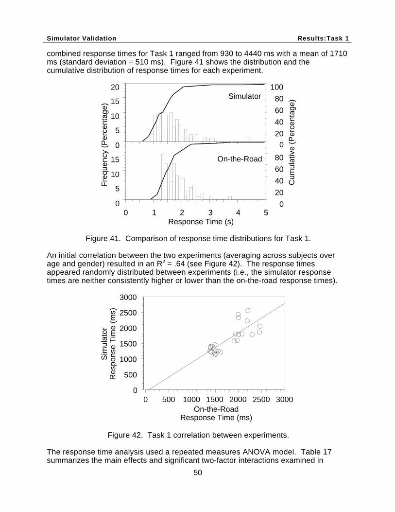
Simulator Validation Results:Task 1
50
combined response times for Task 1 ranged from 930 to 4440 ms with a mean of 1710ms (standard deviation = 510 ms). Figure 41 shows the distribution and thecumulative distribution of response times for each experiment.
020
40
60
80
100
0
20
40
60
80
0
5
10
15
20
0
5
10
15
0 1 2 3 4 5Response Time (s)
Simulator
On-the-Road
Fre
quen
cy (
Per
cent
age)
Cum
ulat
ive
(Per
cent
age)
Figure 41. Comparison of response time distributions for Task 1.
An initial correlation between the two experiments (averaging across subjects overage and gender) resulted in an R2 = .64 (see Figure 42). The response timesappeared randomly distributed between experiments (i.e., the simulator responsetimes are neither consistently higher or lower than the on-the-road response times).
0
500
1000
1500
2000
2500
3000
Sim
ulat
orR
espo
nse
Tim
e (m
s)
0 500 1000 1500 2000 2500 3000On-the-Road
Response Time (ms)
Figure 42. Task 1 correlation between experiments.
The response time analysis used a repeated measures ANOVA model. Table 17summarizes the main effects and significant two-factor interactions examined in
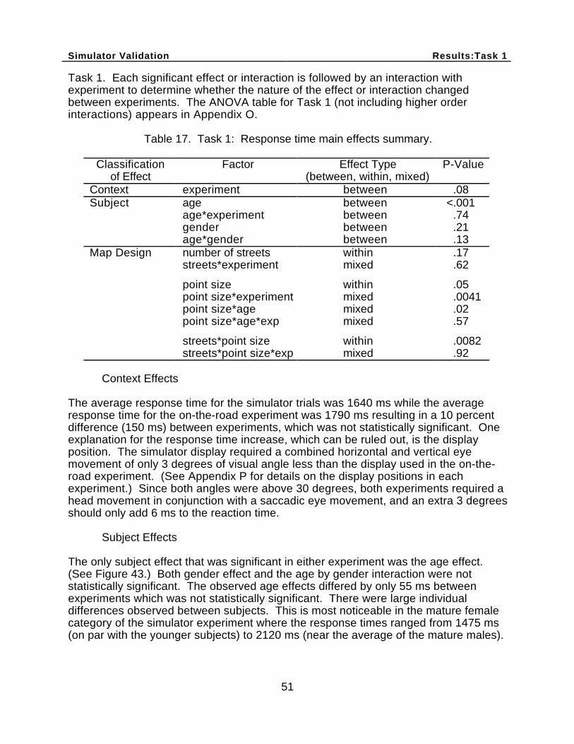
Simulator Validation Results:Task 1
51
Task 1. Each significant effect or interaction is followed by an interaction withexperiment to determine whether the nature of the effect or interaction changedbetween experiments. The ANOVA table for Task 1 (not including higher orderinteractions) appears in Appendix O.
Table 17. Task 1: Response time main effects summary.
Classificationof Effect
Factor Effect Type(between, within, mixed)
P-Value
Context experiment between .08Subject age between <.001
age*experiment between .74gender between .21age*gender between .13
Map Design number of streets within .17streets*experiment mixed .62
point size within .05point size*experiment mixed .0041point size*age mixed .02point size*age*exp mixed .57
streets*point size within .0082streets*point size*exp mixed .92
Context Effects
The average response time for the simulator trials was 1640 ms while the averageresponse time for the on-the-road experiment was 1790 ms resulting in a 10 percentdifference (150 ms) between experiments, which was not statistically significant. Oneexplanation for the response time increase, which can be ruled out, is the displayposition. The simulator display required a combined horizontal and vertical eyemovement of only 3 degrees of visual angle less than the display used in the on-the-road experiment. (See Appendix P for details on the display positions in eachexperiment.) Since both angles were above 30 degrees, both experiments required ahead movement in conjunction with a saccadic eye movement, and an extra 3 degreesshould only add 6 ms to the reaction time.
Subject Effects
The only subject effect that was significant in either experiment was the age effect.(See Figure 43.) Both gender effect and the age by gender interaction were notstatistically significant. The observed age effects differed by only 55 ms betweenexperiments which was not statistically significant. There were large individualdifferences observed between subjects. This is most noticeable in the mature femalecategory of the simulator experiment where the response times ranged from 1475 ms(on par with the younger subjects) to 2120 ms (near the average of the mature males).
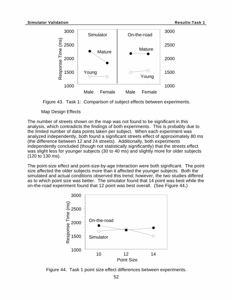
Simulator Validation Results:Task 1
52
1000
1500
2000
2500
3000
Res
pons
e T
ime
(ms)
Male Male FemaleFemale1000
1500
2000
2500
3000Simulator On-the-road
Mature
Young
Mature
Young
Figure 43. Task 1: Comparison of subject effects between experiments.
Map Design Effects
The number of streets shown on the map was not found to be significant in thisanalysis, which contradicts the findings of both experiments. This is probably due tothe limited number of data points taken per subject. When each experiment wasanalyzed independently, both found a significant streets effect of approximately 80 ms(the difference between 12 and 24 streets). Additionally, both experimentsindependently concluded (though not statistically significantly) that the streets effectwas slight less for younger subjects (30 to 40 ms) and slightly more for older subjects(120 to 130 ms).
The point-size effect and point-size-by-age interaction were both significant. The pointsize affected the older subjects more than it affected the younger subjects. Both thesimulated and actual conditions observed this trend; however, the two studies differedas to which point size was better. The simulator found that 14 point was best while theon-the-road experiment found that 12 point was best overall. (See Figure 44.)
1000
1500
2000
2500
3000
Res
pons
e T
ime
(ms)
10 12 14Point Size
On-the-road
Simulator
Figure 44. Task 1 point size effect differences between experiments.
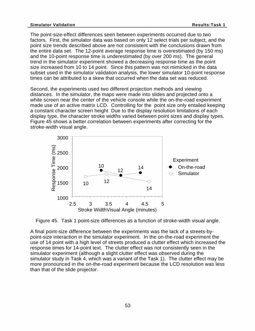
Simulator Validation Results:Task 1
53
The point-size-effect differences seen between experiments occurred due to twofactors. First, the simulator data was based on only 12 select trials per subject, and thepoint size trends described above are not consistent with the conclusions drawn fromthe entire data set. The 12-point average response time is overestimated (by 150 ms)and the 10-point response time is underestimated (by over 200 ms). The generaltrend in the simulator experiment showed a decreasing response time as the pointsize increased from 10 to 14 point. Since this pattern was not mimicked in the datasubset used in the simulator validation analysis, the lower simulator 10-point responsetimes can be attributed to a skew that occurred when the data set was reduced.
Second, the experiments used two different projection methods and viewingdistances. In the simulator, the maps were made into slides and projected onto awhite screen near the center of the vehicle console while the on-the-road experimentmade use of an active matrix LCD. Controlling for the point size only entailed keepinga constant character screen height Due to the display resolution limitations of eachdisplay type, the character stroke widths varied between point sizes and display types.Figure 45 shows a better correlation between experiments after correcting for thestroke-width visual angle.
2.5 3 3.5 4 4.5 51000
1500
2000
2500
3000
Res
pons
e T
ime
(ms)
Stroke WidthVisual Angle (minutes)
10 1214
1012
14SimulatorOn-the-road
Experiment
Figure 45. Task 1 point-size differences as a function of stroke-width visual angle.
A final point-size difference between the experiments was the lack of a streets-by-point-size interaction in the simulator experiment. In the on-the-road experiment theuse of 14 point with a high level of streets produced a clutter effect which increased theresponse times for 14-point text. The clutter effect was not consistently seen in thesimulator experiment (although a slight clutter effect was observed during thesimulator study in Task 4, which was a variant of the Task 1). The clutter effect may bemore pronounced in the on-the-road experiment because the LCD resolution was lessthan that of the slide projector.
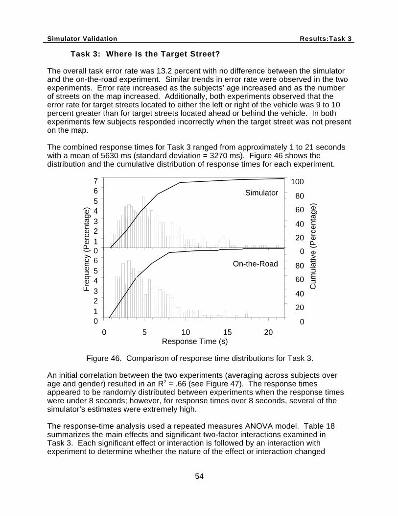
Simulator Validation Results:Task 3
54
Task 3: Where Is the Target Street?
The overall task error rate was 13.2 percent with no difference between the simulatorand the on-the-road experiment. Similar trends in error rate were observed in the twoexperiments. Error rate increased as the subjects’ age increased and as the numberof streets on the map increased. Additionally, both experiments observed that theerror rate for target streets located to either the left or right of the vehicle was 9 to 10percent greater than for target streets located ahead or behind the vehicle. In bothexperiments few subjects responded incorrectly when the target street was not presenton the map.
The combined response times for Task 3 ranged from approximately 1 to 21 secondswith a mean of 5630 ms (standard deviation = 3270 ms). Figure 46 shows thedistribution and the cumulative distribution of response times for each experiment.
01234567
0
20
40
60
80
100
0123456
Fre
quen
cy (
Per
cent
age)
0 5 10 15 20Response Time (s)
0
20
40
60
80
Cum
ulat
ive
(Per
cent
age)
Simulator
On-the-Road
Figure 46. Comparison of response time distributions for Task 3.
An initial correlation between the two experiments (averaging across subjects overage and gender) resulted in an R2 = .66 (see Figure 47). The response timesappeared to be randomly distributed between experiments when the response timeswere under 8 seconds; however, for response times over 8 seconds, several of thesimulator’s estimates were extremely high.
The response-time analysis used a repeated measures ANOVA model. Table 18summarizes the main effects and significant two-factor interactions examined inTask 3. Each significant effect or interaction is followed by an interaction withexperiment to determine whether the nature of the effect or interaction changed
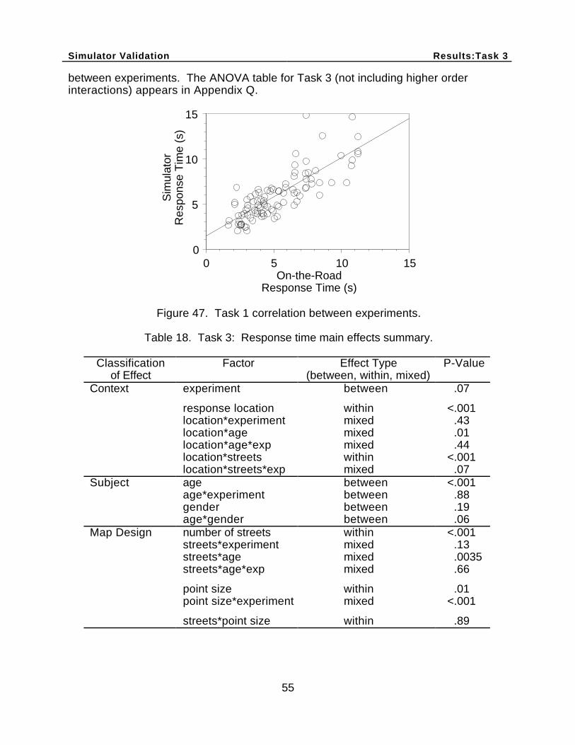
Simulator Validation Results:Task 3
55
between experiments. The ANOVA table for Task 3 (not including higher orderinteractions) appears in Appendix Q.
0
5
10
15
Sim
ulat
orR
espo
nse
Tim
e (s
)
0 5 10 15On-the-Road
Response Time (s)
Figure 47. Task 1 correlation between experiments.
Table 18. Task 3: Response time main effects summary.
Classificationof Effect
Factor Effect Type(between, within, mixed)
P-Value
Context experiment between .07
response location within <.001location*experiment mixed .43location*age mixed .01location*age*exp mixed .44location*streets within <.001location*streets*exp mixed .07
Subject age between <.001age*experiment between .88gender between .19age*gender between .06
Map Design number of streets within <.001streets*experiment mixed .13streets*age mixed .0035streets*age*exp mixed .66
point size within .01point size*experiment mixed <.001
streets*point size within .89
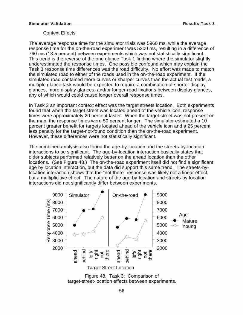
Simulator Validation Results:Task 3
56
Context Effects
The average response time for the simulator trials was 5960 ms, while the averageresponse time for the on-the-road experiment was 5200 ms, resulting in a difference of760 ms (13.5 percent) between experiments which was not statistically significant.This trend is the reverse of the one glance Task 1 finding where the simulator slightlyunderestimated the response times. One possible confound which may explain theTask 3 response time differences was the road difficulty. No effort was made to matchthe simulated road to either of the roads used in the on-the-road experiment. If thesimulated road contained more curves or sharper curves than the actual test roads, amultiple glance task would be expected to require a combination of shorter displayglances, more display glances, and/or longer road fixations between display glances,any of which would could cause longer overall response times.
In Task 3 an important context effect was the target streets location. Both experimentsfound that when the target street was located ahead of the vehicle icon, responsetimes were approximately 20 percent faster. When the target street was not present onthe map, the response times were 50 percent longer. The simulator estimated a 10percent greater benefit for targets located ahead of the vehicle icon and a 25 percentless penalty for the target-not-found condition than the on-the-road experiment.However, these differences were not statistically significant.
The combined analysis also found the age-by-location and the streets-by-locationinteractions to be significant. The age-by-location interaction basically states thatolder subjects performed relatively better on the ahead location than the otherlocations. (See Figure 48.) The on-the-road experiment itself did not find a significantage by location interaction, but the data did support this same trend. The streets-by-location interaction shows that the “not there” response was likely not a linear effect,but a multiplicitive effect. The nature of the age-by-location and streets-by-locationinteractions did not significantly differ between experiments.
Simulator
2000
3000
4000
5000
6000
7000
8000
9000
Res
pons
e T
ime
(ms)
Target Street Location
not
ther
e
ahea
d
behi
nd
left/
right
not
ther
e
ahea
d
behi
nd
left/
right
MatureYoung
Age
On-the-road
2000
3000
4000
5000
6000
7000
8000
9000
Figure 48. Task 3: Comparison oftarget-street-location effects between experiments.

Simulator Validation Results:Task 3
57
Subject Effects
The only subject effect that was significant in either experiment was the age effect.(See Figure 49.) Both gender and the age by gender interaction were not statisticallysignificant. The observed age effects differed by only 130 ms between experiments,which was not statistically significant.
3000
4000
5000
6000
7000
8000
9000R
espo
nse
Tim
e (m
s)
Male MaleFemale Female
Simulator On-the-road
Young
Mature
Young
Mature
3000
4000
5000
6000
7000
8000
9000
Figure 49. Task 3: Comparison of subject effects between experiments.
Map Design Effects
Both experiments found a significant streets effect. The response times increasedapproximately 210 ms per additional street shown on the map. The simulatorexperiment estimated the slope as slightly higher at 230 ms per each additional street,and the on-the-road experiment estimated the slope as slightly lower at 190 ms pereach additional street. This difference was not statistically significant. In addition tothe streets effect, both experiments observed a similar significant streets-by-ageinteraction. The older subjects had relatively more difficulty with 24-street maps thandid younger subjects. (See Figure 50.)
Mature
3000
4000
5000
6000
7000
8000
9000
Res
pons
e T
ime
(ms)
12 24 12 24
Young
3000
4000
5000
6000
7000
8000
9000
Number of Streets
Simulator On-the-road
Age
Figure 50. Task 3: Comparison of the by age interaction between experiments.
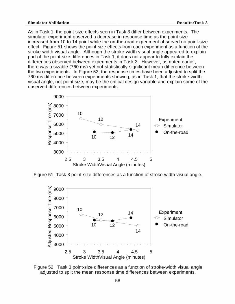
Simulator Validation Results:Task 3
58
As in Task 1, the point-size effects seen in Task 3 differ between experiments. Thesimulator experiment observed a decrease in response time as the point sizeincreased from 10 to 14 point while the on-the-road experiment observed no point-sizeeffect. Figure 51 shows the point-size effects from each experiment as a function of thestroke-width visual angle. Although the stroke-width visual angle appeared to explainpart of the point-size differences in Task 1, it does not appear to fully explain thedifferences observed between experiments in Task 3. However, as noted earlier,there was a sizable (760 ms) yet not-statistically-significant mean difference betweenthe two experiments. In Figure 52, the response times have been adjusted to split the760 ms difference between experiments showing, as in Task 1, that the stroke-widthvisual angle, not point size, may be the critical design variable and explain some of theobserved differences between experiments.
3000
4000
5000
6000
7000
8000
9000
Res
pons
e T
ime
(ms)
2.5 3 3.5 4 4.5 5Stroke WidthVisual Angle (minutes)
10 12
14
1012
14
SimulatorOn-the-road
Experiment
Figure 51. Task 3 point-size differences as a function of stroke-width visual angle.
3000
4000
5000
6000
7000
8000
9000
Adj
uste
d R
espo
nse
Tim
e (m
s)
2.5 3 3.5 4 4.5 5Stroke WidthVisual Angle (minutes)
10 12
1410
12
14
SimulatorOn-the-road
Experiment
Figure 52. Task 3 point-size differences as a function of stroke-width visual angleadjusted to split the mean response time differences between experiments.
Simulator Validation Conclusions
59
Simulator Validation Conclusions
A second accomplishment of this experiment was validating the use of a drivingsimulator to study secondary response-time tasks. The error rates for each task did notdiffer between experiments. For both easy and difficult tasks, the response timesobtained in the simulator showed an initial correlation (r = 0.54) to the response timesobtained on the road. The response times in the two experiments deviated by only 10to 13 percent relative to the mean task response time. For an easy task, one lastingapproximately 1.8 seconds and requiring only a single glance to the display, thesimulator underestimated the response times. For a more difficult task, one lastingover 5 seconds and requiring multiple glances to the display, the simulatoroverestimated the response times.
Since the error between the simulator predictions and the on-the-road response timeswas proportional to the task difficulty (task mean response time), the error may becaused by one of several factors not explored in these experiments. The most likelycause stems from the fact that in comparing the simulator and the on-the-road studies,no attempt was made to match the roads used. The simulator used a virtual road withmore frequent curves and sharper curves than presented in the real world. A moredifficult virtual road could cause the simulator to overestimate the response time in amultiple glance task as the driver is forced to allocate more resources to driving byeither lengthening the interglance interval or adopting a strategy of using an increasednumber of shorter glances.
In validating the driving-simulator predictions, simply verifying the mean responsetimes does not guarantee that the simulator predictions will hold. The two methodsshould agree as to which factors are important and to the relative size and trend ofeach factor. The simulator accurately predicted the age effect within 3 percent of thetask mean, and it predicted the important interactions with age. Likewise, thesimulator’s prediction of the streets effect matched the same effect observed in the on-the-road experiment.
The only effect that differed between experiments was the point-size effect. The point-size effects were relatively small and near the threshold of detectability whencompared with the variability in the experiment. The physical appearance of the text indifferent point sizes was also near the threshold of detectability for some subjects.Although subjects were tested for far visual acuity, the actual maps were presented ata distance of approximately 40 inches, which is somewhere between far and nearacuity. Additionally, only the overall character height was controlled for betweenexperiments. Limitations of the display resolutions changed the character-stroke-widthheights between experiments, and the differing vehicle interiors altered the mountinglocations slightly. These factors accounted for some of the differences found betweenthe simulator and on-the-road experiments and suggest that when dealing with smalleffects or near threshold stimuli, the accuracy of the physical locations and hardwaredisplay capabilities of the simulated system are important considerations to achieve anaccurate prediction.

60
61
REFERENCES
Brooks, A. and Green, P. (1998). Map Design: A Simulator Evaluation of the Time toRead Electronic Navigation Displays (Technical Report UMTRI-98-7), AnnArbor, MI: The University of Michigan Transportation Research Institute.
DeLorme Mapping (1993). Street Atlas USA , version 2.0, Freeport, ME: DelormeMapping.
Dingus, T., McGehee, D., Hulse, M., Jahns, S., Manakkal, N., Mollenhauer, M., andFleischman, R. (1995). TravTek Evaluation Task C3 - Camera Car Study (Technical Report FHWA-RD-94-076), McLean, VA: U. S. Department ofTransportation, Federal Highway Administration.
Evans, C.K. (1994). Unusual and Popular Baby Names , Lincolnwood, IL: PublicationsInternational.
Goodman, M., Bents, F.D., Tijerina, L., Wierwille, W., Lerner, N., and Benel, D. (1997).An Investigation of the Safety Implications of Wireless Communications inVehicles (Technical Report DOT HS 808 635), Washington, D.C.: U.S.Department of Transportation, National Highway Traffic Safety Administration.
Green, P. (1992). American Human Factors Research On In-Vehicle NavigationSystems (Technical Report UMTRI-92-47), Ann Arbor, MI: The University ofMichigan Transportation Research Institute.
Green, P., Williams, M., Hoekstra, E., George, K., and Wen, C. (1993). Initial On-the- Road Tests of Driver Information System Interfaces: Examination of Navigation,Traffic Information, IVSAWS, and Vehicle Monitoring (Technical report UMTRI-93-32), Ann Arbor, MI: The University of Michigan Transportation ResearchInstitute.
Green, P., Hoekstra, E., and Williams, M. (1993). On-The-Road Tests of DriverInterfaces: Examination of a Navigation System and a Car Phone (TechnicalReport UMTRI-93-35), Ann Arbor, MI: The University of Michigan TransportationResearch Institute.
Green, P. (1997). Potential Safety Impacts of Automotive Navigation Systems Paper presented at the Automotive Land Navigation Conference, June 18,1997, Detroit, Michigan.
Green, P. (1998). Reading Electronic Area Maps: An Annotated Bibliography (Technical Report UMTRI-98-38), Ann Arbor, MI: The University of Michigan Transportation Research Institute.
Hada, H. (1994). Drivers' Visual Attention to In-Vehicle Displays: Effects of DisplayLocation and Road Types (Technical Report UMTRI-94-9), Ann Arbor, MI: TheUniversity of Michigan Transportation Research Institute.

62
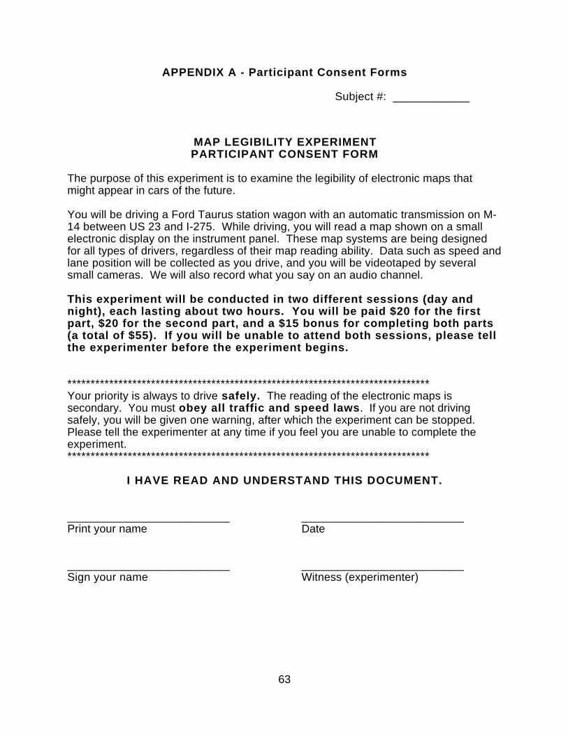
63
APPENDIX A - Participant Consent Forms
Subject #: ____________
MAP LEGIBILITY EXPERIMENTPARTICIPANT CONSENT FORM
The purpose of this experiment is to examine the legibility of electronic maps thatmight appear in cars of the future.
You will be driving a Ford Taurus station wagon with an automatic transmission on M-14 between US 23 and I-275. While driving, you will read a map shown on a smallelectronic display on the instrument panel. These map systems are being designedfor all types of drivers, regardless of their map reading ability. Data such as speed andlane position will be collected as you drive, and you will be videotaped by severalsmall cameras. We will also record what you say on an audio channel.
This experiment will be conducted in two different sessions (day andnight), each lasting about two hours. You will be paid $20 for the firstpart, $20 for the second part, and a $15 bonus for completing both parts(a total of $55). If you will be unable to attend both sessions, please tellthe experimenter before the experiment begins.
******************************************************************************Your priority is always to drive safely. The reading of the electronic maps issecondary. You must obey all traffic and speed laws. If you are not drivingsafely, you will be given one warning, after which the experiment can be stopped.Please tell the experimenter at any time if you feel you are unable to complete theexperiment.******************************************************************************
I HAVE READ AND UNDERSTAND THIS DOCUMENT.
_________________________ _________________________Print your name Date
_________________________ _________________________Sign your name Witness (experimenter)
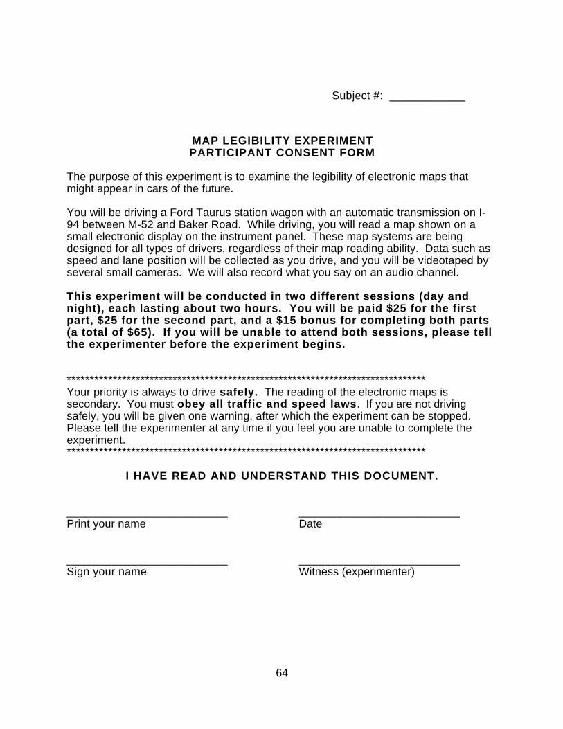
64
Subject #: ____________
MAP LEGIBILITY EXPERIMENTPARTICIPANT CONSENT FORM
The purpose of this experiment is to examine the legibility of electronic maps thatmight appear in cars of the future.
You will be driving a Ford Taurus station wagon with an automatic transmission on I-94 between M-52 and Baker Road. While driving, you will read a map shown on asmall electronic display on the instrument panel. These map systems are beingdesigned for all types of drivers, regardless of their map reading ability. Data such asspeed and lane position will be collected as you drive, and you will be videotaped byseveral small cameras. We will also record what you say on an audio channel.
This experiment will be conducted in two different sessions (day andnight), each lasting about two hours. You will be paid $25 for the firstpart, $25 for the second part, and a $15 bonus for completing both parts(a total of $65). If you will be unable to attend both sessions, please tellthe experimenter before the experiment begins.
******************************************************************************Your priority is always to drive safely. The reading of the electronic maps issecondary. You must obey all traffic and speed laws. If you are not drivingsafely, you will be given one warning, after which the experiment can be stopped.Please tell the experimenter at any time if you feel you are unable to complete theexperiment.******************************************************************************
I HAVE READ AND UNDERSTAND THIS DOCUMENT.
_________________________ _________________________Print your name Date
_________________________ _________________________Sign your name Witness (experimenter)
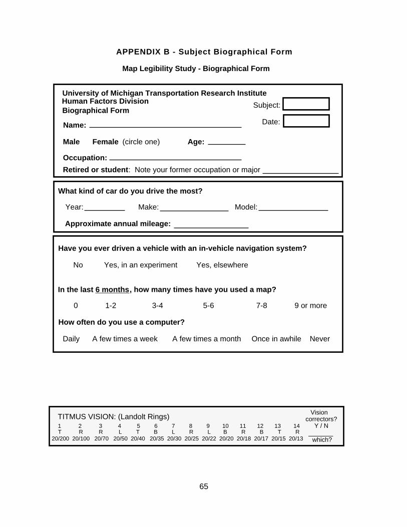
65
APPENDIX B - Subject Biographical Form
Name:
Male Female (circle one) Age:
Occupation:
What kind of car do you drive the most?
Year: Make: Model:
Approximate annual mileage:
Have you ever driven a vehicle with an in-vehicle navigation system? No Yes, in an experiment Yes, elsewhere
In the last 6 months, how many times have you used a map?
0 1-2 3-4 5-6 7-8 9 or more
How often do you use a computer? Daily A few times a week A few times a month Once in awhile Never
Retired or student: Note your former occupation or major
Date:
Subject:
University of Michigan Transportation Research InstituteHuman Factors Division Biographical Form
1 2 3 4 5 6 7 8 9 10 11 12 13 14 T R R L T B L R L B R B T R 20/200 20/100 20/70 20/50 20/40 20/35 20/30 20/25 20/22 20/20 20/18 20/17 20/15 20/13
TITMUS VISION: (Landolt Rings) Vision correctors? Y / N _______ which?
Map Legibility Study - Biographical Form

66
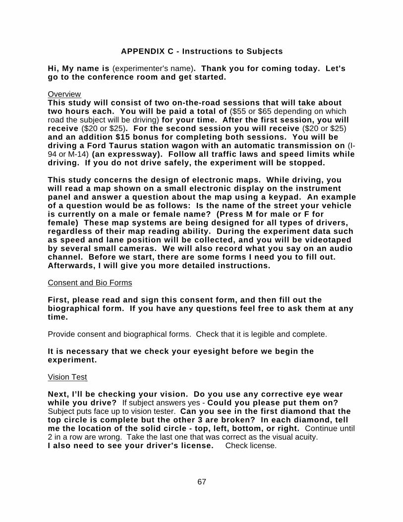
67
APPENDIX C - Instructions to Subjects
Hi, My name is (experimenter's name). Thank you for coming today. Let'sgo to the conference room and get started.
OverviewThis study will consist of two on-the-road sessions that will take abouttwo hours each. You will be paid a total of ($55 or $65 depending on whichroad the subject will be driving) for your time. After the first session, you willreceive ($20 or $25). For the second session you will receive ($20 or $25)and an addition $15 bonus for completing both sessions. You will bedriving a Ford Taurus station wagon with an automatic transmission on (I-94 or M-14) (an expressway). Follow all traffic laws and speed limits whiledriving. If you do not drive safely, the experiment will be stopped.
This study concerns the design of electronic maps. While driving, youwill read a map shown on a small electronic display on the instrumentpanel and answer a question about the map using a keypad. An exampleof a question would be as follows: Is the name of the street your vehicleis currently on a male or female name? (Press M for male or F forfemale) These map systems are being designed for all types of drivers,regardless of their map reading ability. During the experiment data suchas speed and lane position will be collected, and you will be videotapedby several small cameras. We will also record what you say on an audiochannel. Before we start, there are some forms I need you to fill out.Afterwards, I will give you more detailed instructions.
Consent and Bio Forms
First, please read and sign this consent form, and then fill out thebiographical form. If you have any questions feel free to ask them at anytime.
Provide consent and biographical forms. Check that it is legible and complete.
It is necessary that we check your eyesight before we begin theexperiment.
Vision Test
Next, I’ll be checking your vision. Do you use any corrective eye wearwhile you drive? If subject answers yes - Could you please put them on?Subject puts face up to vision tester. Can you see in the first diamond that thetop circle is complete but the other 3 are broken? In each diamond, tellme the location of the solid circle - top, left, bottom, or right. Continue until2 in a row are wrong. Take the last one that was correct as the visual acuity.I also need to see your driver's license. Check license.
68
At the test vehicle
Let me reiterate a few important points from the consent form. First of all,driving safely is your main priority. If you feel unsafe or unable to makeany turn, please don't. Second, if you are uncomfortable or wish to stopat any time, please let me know right away. You are expected to obey allspeed limits and driving laws. The speed limit on M-14 is 65 mphthrough the section we will be driving, but we ask that you maintain 55mph during the experiment.
Please fasten your seat belt, adjust the seat, mirrors, steering wheelheight, as you feel necessary.
•adjust the car seat, steering wheel height, and side- and rear-view mirrors.•Fasten seat belt.•Point out climate controls, and radio volume knob.•Adjust eye fixation camera once subject is comfortable.•Remind about following speed limit.•After Vehicle is started, turn on computer and adjust rear monitor.•Start up ToyotaMap by double clicking on the icon.
Overview while Still At UMTRI (sit up front at this point and make sure camera’s focused)
This is a study to determine how different features affect the ease ofreading a map. Some of these factors of interest are the street name fontsize and the number of streets on the map.
For the first stretch you will just practice driving with your left hand onthe wheel and your right hand on the keypad while familiarizing yourselfwith the route. Subsequent trips will add either practice tasks orexperimental tasks using the keypad to answer questions about thedisplayed map. Each task will have a specific question associated withthe entire task. Each task consists of 24 trials.
As an example of what to expect, for your first practice session, you’ll beshown one name on the display screen to your right and then answer thequestion of whether that name is male or female.
Point out Display and Keypad.Adjust Keypad and arm rests so that the driver is comfortable.Show Task one Fingering and how to steady hand.
For Example:Play Demo of Practice 1 (Command Key 1)Adjust Radio Volume
69
As you noticed a "ding" will sound each time before the name appears tonotify you of a change in the map. The name will either be a male orfemale name. Your task is to determine whether the name is male orfemale and to respond by pressing the appropriate button on the keypadto your right. Quickly press and release the left key (marked "M") if thename you see is male, such as John. If the name is female, such asJane, press the key marked "F."
Subject responds correctly.
A correct answer is responded to with a "simple beep". An incorrectanswer will be responded to with a "buzzer" tone. If you answerincorrectly, do not try to respond again; just move on to the next slide.
Replay Demo of Practice 1 (Command Key 1)Subject responds incorrectly.
I will briefly demonstrate each of the remaining tasks for you now, butyou need not memorize the specifics. I will go over each task again justprior to its start. The first task, Task 1, will be to decide the gender of thestreet on which your vehicle icon is traveling.
Play Demo of Task 1 (Command Key 2)
Again, a "ding" will sound and a map will appear. Locate your vehicleicon. Locate the street name. Decide whether that name is male orfemale. Respond with M or F on the keypad.
Note: At night, show the subject where the display brightness/contrast dial is andhave the subject adjust it at this point to his or her liking.
The next task, Task 2, will have the same responses, "M" and "F" as taskone, but will also add the next key "Not there." You will be given the"number" of a cross street to locate on the map. The map will appearafter the number is read (There is no "ding" this time).
Play Demo of Task 2 (Command Key 3)
Locate your vehicle icon and the street you are on. Count up thespecified number of cross streets. Note that a cross street is defined asintersecting the street you are on or more simply, any street that you canturn onto. When you find the specified cross street locate its name andrespond with answers for this task are M (male), F (female), or 0 (notthere).
Play Demo of Task 2 (Command Keys 4)
In the next two sets you will need to change your fingering position.

70
Show new fingering and how to steady hand.
You will be responding Ahead (middle finger), Behind (middle finger), Left(index finger), Right (ring finger), or Not There (middle finger).
Play Demo of Practice 2 (Command Key 5)
In this practice set a "ding" will sound and a map will appear. Find thebolded street on the map. Determine its position relative to your vehicleicon and respond. Note that Ahead and Behind only apply to crossstreets, streets that intersects the street your on which your vehicle iconis traveling.
Play Demo of Practice 2 (Command Keys 6 and 7)
The final task uses the same response keys only this time you will hearthe name of a street instead of a "ding."
Play Demo of Task 3 (Command Key 8)
The map will appear after the name is read. Search the map and locatethat street name. Decide and respond with that street's relative locationto your vehicle icon with either "Ahead, Behind, Right, Left, or NotThere."
Play Demo of Task 3 (Command Keys 9 and 0)
After Each task I will ask you to rate the difficulty of the task and how youfelt during the task on a scale from 1 to 5 with one being...1. No Interference with Driving, Very Safe.2. Some Interference, but Safe.3. Some Interference, Sometimes Unsafe.4. Much Interference, Unsafe.5. Extreme Interference, Very Unsafe.
Remember, I will go over each task in detail before just prior to startingthe task, but for now do you have any questions in general about theexperiment? If not, we can drive out to M-14 and begin.
Give subject directions to M-14.Fill in subject data sheet for the file header.
On Road Section 1
•Turn on VCR after passing (Exit 10 for M-14 or Baker Road for I-94)
OK, at this point I'm going to begin recording. I'd like you place yourright hand on the keypad and drive with your left hand only (unless ofcourse it's an emergency). Just relax and just drive normally. We will be

71
getting off the expressway at Beck Road which is about 10 miles ahead.Maintain 55 mph for this stretch of road.
•Exit the expressway at (Beck Road or US 52)•Give good directions on getting back on the expressway in the correct direction.
On the Scale from 1 to 5, how would you rate this task?
•Clarrify rating scale if needed. Record response in ToyotaMap comment section.
On Road Section 2
On the next stretch of road, I'm going to start the first practice task. Asyou will remember from the demonstration, in this task you will hear a"ding" and a name will appear in the center of the display to your right.Read the name and decide its gender. Your response will be either M formale or F for female.
Try not to look down at the keypad to respond, and remember, if youanswer incorrectly do not worry or try to answer again. Just note it andmove on. Also try not to look at the screen until you hear the "ding." Usethe time between maps to concentrate on driving and on checking yourmirrors.
REMEMBER, your primary task is to maintain control of the vehicle anddrive safely at all times. Reading the display and responding areSECONDARY tasks.
Once you have merged with traffic and are maintaining a constant speedbetween 55 and 65 mph, position your hand comfortably on the keypadand I will begin the task.
Any Questions?
•Begin Practice Task 1
Note: Use the Pause/Resume Feature (Command P/R) to pause the task during ablack screen whenever traffic is merging from an on-ramp or whenever cars are pulledover on the right shoulder or any other distractions (Cops, Tow Trucks, Sudden BrakeLights Ahead, etc.). Make a note on scratch paper of the trial you paused and thereason for the pause. Then enter this information into the computer at the end of thetask if possible.
•End Practice Task 1
On the Scale from 1 to 5, how would you rate this task?

72
On Road Section 3
The next task will be very similar to the last practice. You will hear a"ding" and a map will appear on the screen. Locate your vehicle icon (ablack arrow). Find the name of the street it is on. Decided whether thatname is male or female and respond accordingly.
Any Questions?
When you have merged with traffic and reached a steady speed between55 and 65 mph we will begin the task.
•Begin Task 1•End Task 1
On the Scale from 1 to 5, how would you rate this task?
On Road Section 4
In the next task, you will be given the "number" of a cross street and thena map will appear. Locate your vehicle icon. Find the designated crossstreet. Decide whether that street name is Male, Female or whether thatstreet is not on the map. You will have the same responses as the lasttask only adding the "Not There" response. If you need the number of thecross street repeated, just ask.
This task is a little bit more challenging than the last two, make sure youfocus on driving safely at all times.
Any Questions?
•Begin Task 2•End Task 2
Note: To Replay the Voice Sample press (Command V).On the Scale from 1 to 5, how would you rate this task?
On Road Section 5
In this next task I would like you to change your finger position from the"Male/Female" keys to the "Arrow Keys." You will probably want to pickup the keypad and move it down closer to you for more comfort. Goahead and adjust that at your convenience.
In this practice task, you will hear a "ding" and a map will appear.Search the map for a bolded street. Determine that street's positionrelative to your vehicle icon. Respond with "Ahead, Behind, Left, Right,or Not There." Try to learn the keypad and responses so that you do notneed to look down at it in order to respond.

73
Any Questions?
•Begin Practice Task 2•End Practice Task 2
On the Scale from 1 to 5, how would you rate this task?
On Road Section 6
The next task will be very similar to the last task only this time you will begiven the name of a street. After the name is spoken, a map will appearon the screen. Search the map for the named street and decide thatstreet's location relative to your vehicle icon. Respond with eitherAhead, Behind, Left, Right or "Not There." You should not need to lookdown at the keypad in order to respond.
Be aware that this task may be challenging and you may have a tendencyto ignore your driving responsibilities as you become engulfed in thetask. Remember that your PRIMARY responsibility is to drive safely andthat should take precedence over responding to the maps.
Any Questions?
•Begin Task 3•End Task 3
Note: To Replay the Voice Sample press (Command V)
On the Scale from 1 to 5, how would you rate this task?
At this point we are finished with the experiment. You will probably wantto accelerate up to the posted speed limit and move over to the left laneso that you can take the (US 23 South or M-14 East Exit) and head back toUMTRI.
Save Data FileCopy Data File to a Floppy DiskShut down the computer and turn off the power inverter.
At UMTRI
If you could come up to the office with me so I can fill out the paymentform and get you your money for today.
Fill out forms.
Thank you for participating today, I will see you sometime next week forthe second session.

74
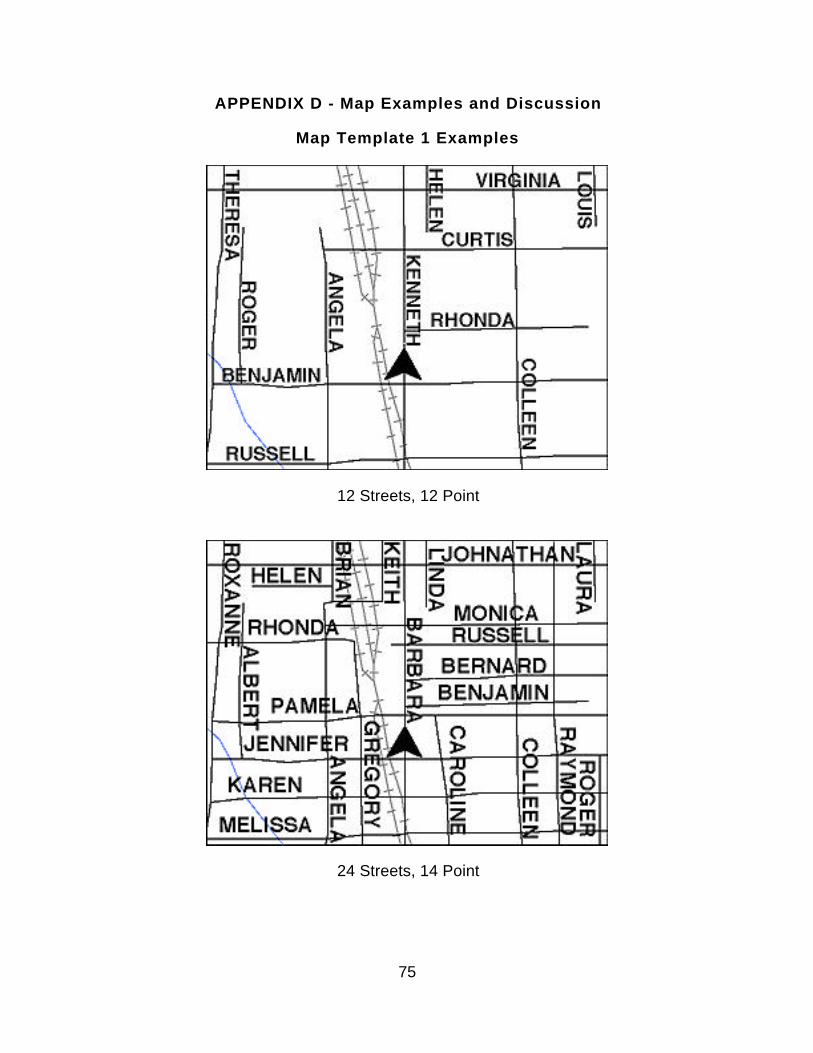
75
APPENDIX D - Map Examples and Discussion
Map Template 1 Examples
12 Streets, 12 Point
24 Streets, 14 Point
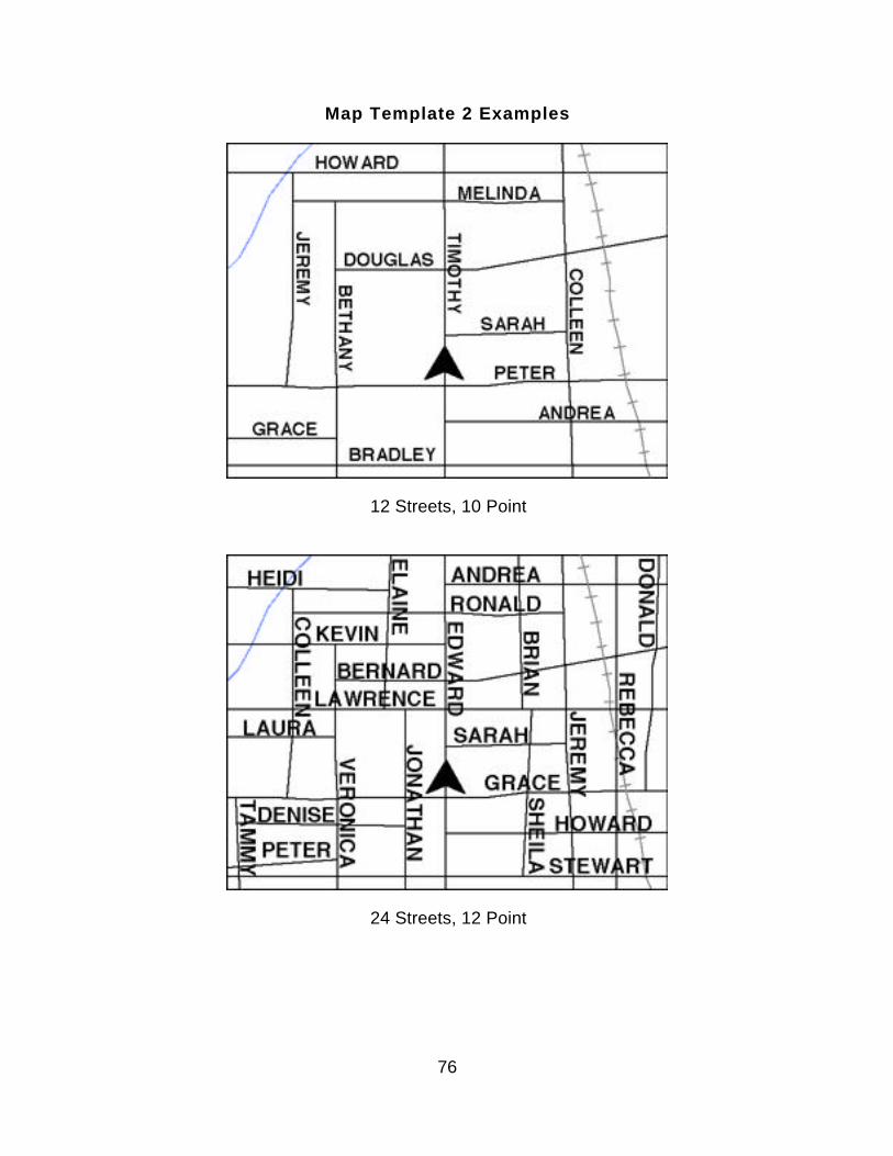
76
Map Template 2 Examples
12 Streets, 10 Point
24 Streets, 12 Point
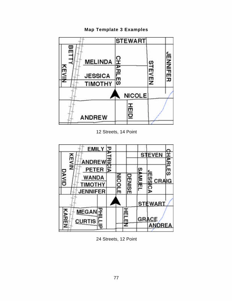
77
Map Template 3 Examples
12 Streets, 14 Point
24 Streets, 12 Point
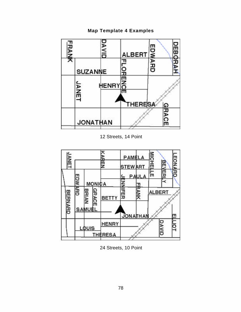
78
Map Template 4 Examples
12 Streets, 14 Point
24 Streets, 10 Point
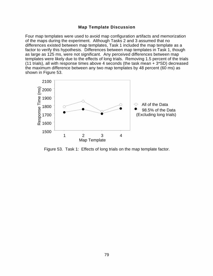
79
Map Template Discussion
Four map templates were used to avoid map configuration artifacts and memorizationof the maps during the experiment. Although Tasks 2 and 3 assumed that nodifferences existed between map templates, Task 1 included the map template as afactor to verify this hypothesis. Differences between map templates in Task 1, thoughas large as 125 ms, were not significant. Any perceived differences between maptemplates were likely due to the effects of long trials. Removing 1.5 percent of the trials(11 trials), all with response times above 4 seconds (the task mean + 3*SD) decreasedthe maximum difference between any two map templates by 48 percent (60 ms) asshown in Figure 53.
1500
1600
1700
1800
1900
2000
2100
Res
pons
e T
ime
(ms)
1 2 3 4Map Template
98.5% of the Data(Excluding long trials)
All of the Data
Figure 53. Task 1: Effects of long trials on the map template factor.

80

81
APPENDIX E - Experimental Conditions by Task
Practice 1 Experimental Conditions
Slide # Response Point Name Start1 Male 10 Bruce Start 12 Female 12 Gloria3 Male 14 Elliot4 Male 10 Benjamin5 Male 12 Samuel6 Female 10 Melinda Start 27 Female 14 Charlotte8 Female 10 Marie9 Male 12 Albert10 Female 10 Heidi11 Female 14 Victoria Start 312 Male 10 Dennis13 Female 12 Judith14 Male 14 Walter15 Female 14 Donna16 Female 12 Angela Start 417 Male 10 Brian18 Male 14 Curtis19 Female 12 Laura20 Male 14 Phillip21 Female 10 Emily Start 522 Male 12 Clifford23 Male 14 Russell24 Female 12 Rhonda
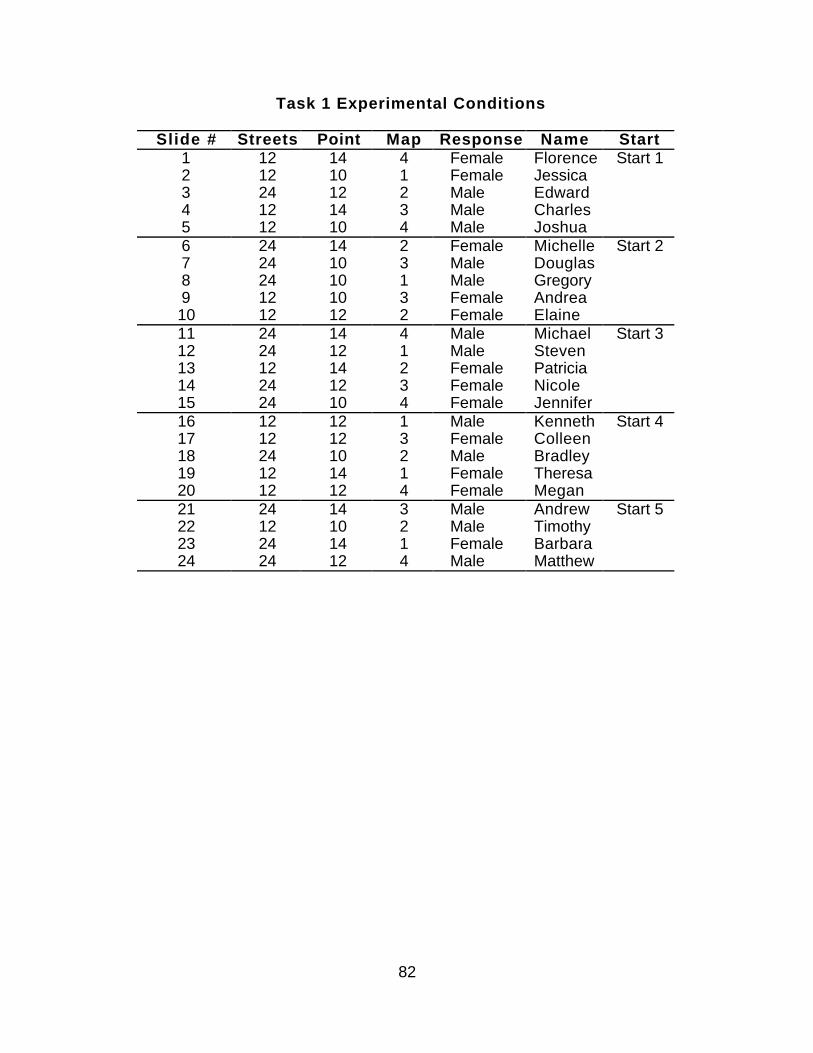
82
Task 1 Experimental Conditions
Slide # Streets Point Map Response Name Start1 12 14 4 Female Florence Start 12 12 10 1 Female Jessica3 24 12 2 Male Edward4 12 14 3 Male Charles5 12 10 4 Male Joshua6 24 14 2 Female Michelle Start 27 24 10 3 Male Douglas8 24 10 1 Male Gregory9 12 10 3 Female Andrea10 12 12 2 Female Elaine11 24 14 4 Male Michael Start 312 24 12 1 Male Steven13 12 14 2 Female Patricia14 24 12 3 Female Nicole15 24 10 4 Female Jennifer16 12 12 1 Male Kenneth Start 417 12 12 3 Female Colleen18 24 10 2 Male Bradley19 12 14 1 Female Theresa20 12 12 4 Female Megan21 24 14 3 Male Andrew Start 522 12 10 2 Male Timothy23 24 14 1 Female Barbara24 24 12 4 Male Matthew
83
Task 2 Experimental Conditions
Slide # Streets Point Map Response X-Street Name Start1 24 14 2 Male 6 Nathan Start 12 12 10 1 Not There 4 Not There3 12 14 3 Male 4 Joseph4 24 12 3 Not There 6 Not There5 12 10 2 Female 1 Denise6 12 10 3 Female 4 Bethany Start 27 24 14 1 Male 3 Jonathan8 24 14 4 Not There 6 Not There9 12 12 2 Female 4 Margaret10 24 12 4 Female 1 Paula11 12 12 4 Male 3 James Start 312 24 14 3 Female 1 Monica13 12 14 1 Female 1 Melissa14 24 12 2 Male 3 Joshua15 12 12 1 Not There 4 Not There16 24 10 3 Male 3 Richard Start 417 12 10 4 Female 3 Pamela18 24 10 4 Not There 6 Not There19 24 12 1 Male 6 Robert20 12 12 3 Female 1 Grace21 24 10 1 Female 6 Caroline Start 522 12 14 2 Male 3 Jeremy23 24 10 2 Male 1 Marvin24 12 14 4 Not There 4 Not There
84
Practice 2 Experimental Conditions
Slide # Streets Map Response Start1 12 3 Ahead Start 12 24 1 Left3 24 4 Not There4 12 2 Behind5 24 2 Not There6 24 4 Left Start 27 12 3 Ahead8 24 3 Not There9 12 1 Behind
10 24 1 Ahead11 24 4 Right Start 312 24 2 Behind13 12 2 Not There14 12 1 Right15 12 4 Behind16 12 3 Ahead Start 417 12 2 Not There18 12 4 Right19 24 3 Ahead20 12 4 Not There21 24 2 Behind Start 522 12 1 Not There23 24 3 Ahead24 24 1 Behind
85
Task 3 Experimental Conditions
Slide # Streets Point Map Response Name Start1 12 12 3 Right Jessica Start 12 12 10 4 Behind Robert3 24 14 3 Ahead Timothy4 24 12 1 Not There Donna5 24 12 4 Ahead Jonathan6 24 12 3 Left Martin Start 27 12 14 3 Not There Bradley8 12 14 4 Right Angela9 24 10 2 Behind Tammy
10 12 12 2 Not There Michelle11 12 10 2 Ahead Douglas Start 312 24 14 2 Behind Denise13 24 14 1 Not There Craig14 12 10 1 Left Monica15 24 12 2 Behind Stewart16 12 12 4 Ahead James Start 417 24 10 1 Right Sarah18 12 10 3 Not There Karen19 12 12 1 Behind Curtis20 24 10 4 Ahead Thomas21 12 14 2 Behind Melinda Start 522 24 14 4 Left Nicole23 24 10 3 Not There Colleen24 12 14 1 Ahead Jeffery

86
1992 Ford Taurus Station Wagon
Mac Driver's Display - MitsubishiDU-9450M 5" Active Matrix LCD
Panasonic AG-5700 Super VHS VCR
700 Watt Power InverterPowerStar Model UPG 700
Kensington Numeric Keypad
Low Light Subject Camera Panasonic WV - BP310
Speedometer Camera Panasonic GP-KS5162H
Low Light Scene Camera Panasonic WV - BP310
Mac Display - MitsubishiDU-5650 5.5" Active Matrix LCD
VCR/PC Display - MitsubishiDU-5650 5.5" Active Matrix LCD
Piezometric MicrophoneCrown PZM-30 RB
Adesso Tru-Form MacKeyboard & Pointer
Macintosh Sound OutSony CPA-9 CD to Tape Car Connecting Pack
Microphone Phantom PowerCrown PH-1 18V Battery Supply
PC VGA ConverterPresentor TV-View
Radio Shack AC to 12 V DCPower Inverter
Panasonic GP-KS162Camera Controller Box
80486 DX PC (not used)16 MB RAM DOS 6.22
(2) 2-way Video SplittersVicon Model V270SP
Mac RGB ConverterPresentor TV-View
Macintosh PowerPC Model 7100/80 AVSystem 7.5.5 16 MB RAM2X CDROM & 2 Video Cards
APPENDIX F - Test Vehicle Illustrations
87

88
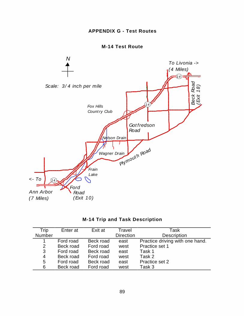
89
APPENDIX G - Test Routes
M-14 Test Route
Frain Lake
Nelson Drain
Wagner Drain
Fox Hills Country Club
Bec
k Road
(Exi
t 1
8)
Ford Road (Exit 10)
<- To
Ann Arbor(7 Miles)
Plymouth Road
14
14
14
Gotfredson Road
NTo Livonia ->(4 Miles)
Scale: 3/4 inch per mile
M-14 Trip and Task Description
TripNumber
Enter at Exit at TravelDirection
TaskDescription
1 Ford road Beck road east Practice driving with one hand.2 Beck road Ford road west Practice set 13 Ford road Beck road east Task 14 Beck road Ford road west Task 25 Ford road Beck road east Practice set 26 Beck road Ford road west Task 3
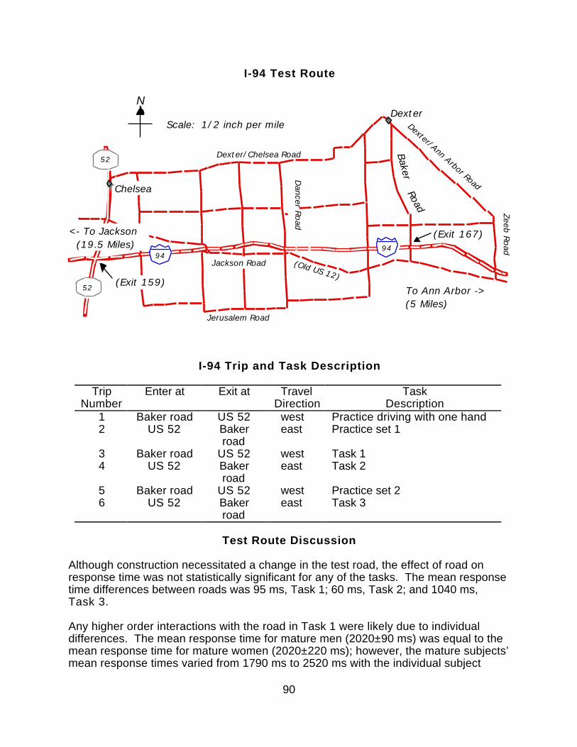
90
I-94 Test Route
Chelsea
Dexter
5252525252
5252525252
Zeeb R
oad
To Ann Arbor ->(5 Miles)
Dexter/Ann Arbor Road
Jerusalem Road
Dexter/Chelsea Road
Dancer R
oad
Jackson Road (Old US 12)
N
Baker
Road
(Exit 167)
(Exit 159)
9494
<- To Jackson (19.5 Miles)
Scale: 1/2 inch per mile
I-94 Trip and Task Description
TripNumber
Enter at Exit at TravelDirection
TaskDescription
1 Baker road US 52 west Practice driving with one hand2 US 52 Baker
roadeast Practice set 1
3 Baker road US 52 west Task 14 US 52 Baker
roadeast Task 2
5 Baker road US 52 west Practice set 26 US 52 Baker
roadeast Task 3
Test Route Discussion
Although construction necessitated a change in the test road, the effect of road onresponse time was not statistically significant for any of the tasks. The mean responsetime differences between roads was 95 ms, Task 1; 60 ms, Task 2; and 1040 ms,Task 3.
Any higher order interactions with the road in Task 1 were likely due to individualdifferences. The mean response time for mature men (2020±90 ms) was equal to themean response time for mature women (2020±220 ms); however, the mature subjects’mean response times varied from 1790 ms to 2520 ms with the individual subject

91
means being distributed at either the upper or lower end of the spectrum. Figure 54shows that in Task 1 the two faster women both drove on one road (I-94) rather thanbeing distributed across roads as in the mature male category.
95%ConfidenceInterval
1000
1500
2000
2500
3000R
espo
nse
Tim
e (m
s)
Men Women Men WomenYoung Mature
I-94M-14
Figure 54. Task 1: Subjects’ mean response times.
As in Task 1, any road effects seen in Task 3 probably reflect individual subjectdifferences. Figure 55 shows that the overall difference between roads (1040 ms) islargely due to the individual differences between the mature women who drove eachroad. Excluding the mature women from the analysis, the difference between M-14and I-94 drops by 61 percent to only 400 ms.
2000
3000
4000
5000
6000
7000
8000
9000
10000
Res
pons
e T
ime
(ms)
I-94M-14
Men Women Men WomenYoung Mature
2
2
95%ConfidenceInterval
Figure 55. Task 3: Subjects’ mean response times.

92
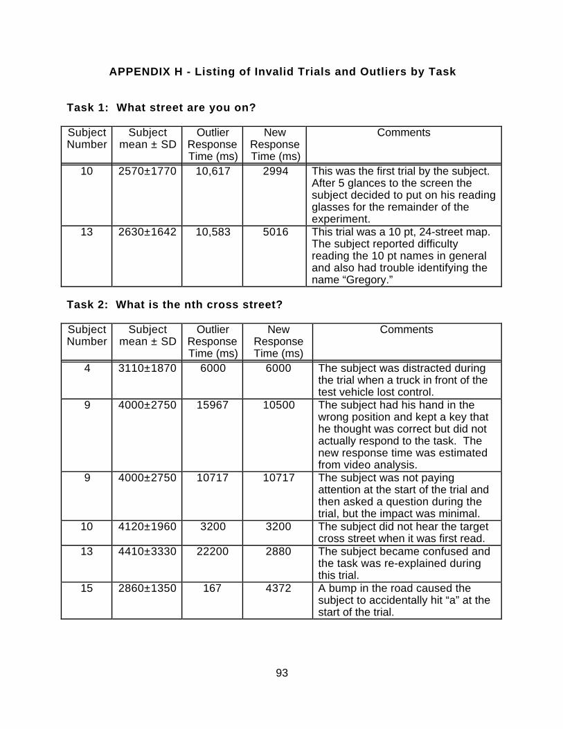
93
APPENDIX H - Listing of Invalid Trials and Outliers by Task
Task 1: What street are you on?
SubjectNumber
Subjectmean ± SD
OutlierResponseTime (ms)
NewResponseTime (ms)
Comments
10 2570±1770 10,617 2994 This was the first trial by the subject.After 5 glances to the screen thesubject decided to put on his readingglasses for the remainder of theexperiment.
13 2630±1642 10,583 5016 This trial was a 10 pt, 24-street map.The subject reported difficultyreading the 10 pt names in generaland also had trouble identifying thename “Gregory.”
Task 2: What is the nth cross street?
SubjectNumber
Subjectmean ± SD
OutlierResponseTime (ms)
NewResponseTime (ms)
Comments
4 3110±1870 6000 6000 The subject was distracted duringthe trial when a truck in front of thetest vehicle lost control.
9 4000±2750 15967 10500 The subject had his hand in thewrong position and kept a key thathe thought was correct but did notactually respond to the task. Thenew response time was estimatedfrom video analysis.
9 4000±2750 10717 10717 The subject was not payingattention at the start of the trial andthen asked a question during thetrial, but the impact was minimal.
10 4120±1960 3200 3200 The subject did not hear the targetcross street when it was first read.
13 4410±3330 22200 2880 The subject became confused andthe task was re-explained duringthis trial.
15 2860±1350 167 4372 A bump in the road caused thesubject to accidentally hit “a” at thestart of the trial.
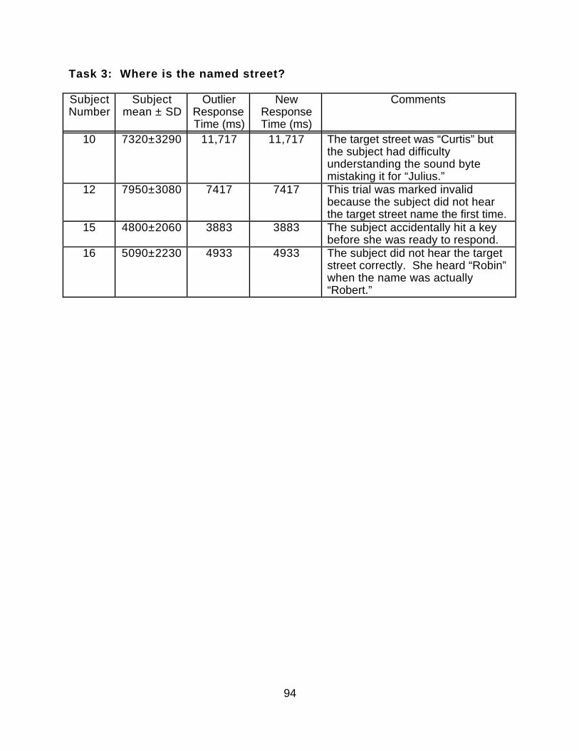
94
Task 3: Where is the named street?
SubjectNumber
Subjectmean ± SD
OutlierResponseTime (ms)
NewResponseTime (ms)
Comments
10 7320±3290 11,717 11,717 The target street was “Curtis” butthe subject had difficultyunderstanding the sound bytemistaking it for “Julius.”
12 7950±3080 7417 7417 This trial was marked invalidbecause the subject did not hearthe target street name the first time.
15 4800±2060 3883 3883 The subject accidentally hit a keybefore she was ready to respond.
16 5090±2230 4933 4933 The subject did not hear the targetstreet correctly. She heard “Robin”when the name was actually“Robert.”
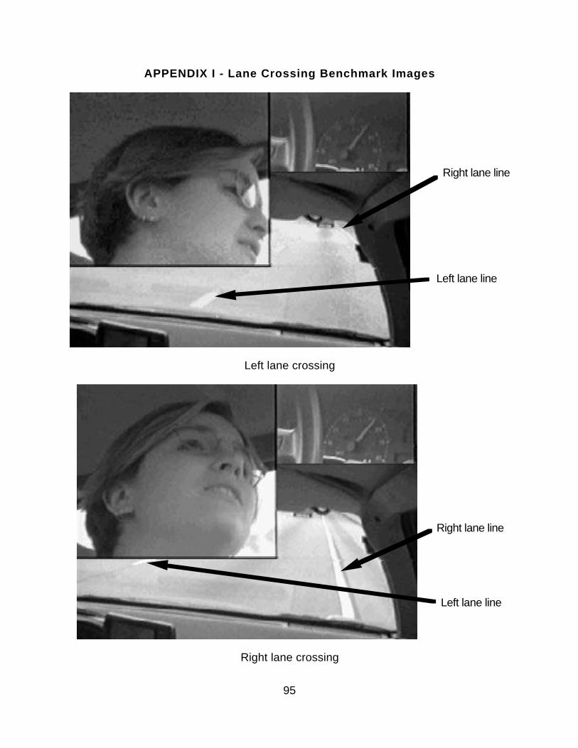
95
APPENDIX I - Lane Crossing Benchmark Images
Right lane line
Left lane line
Left lane crossing
Left lane line
Right lane line
Right lane crossing

96
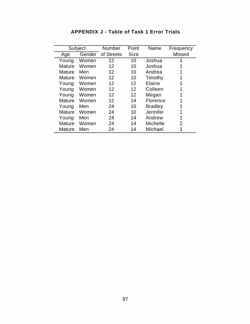
97
APPENDIX J - Table of Task 1 Error Trials
Subject Number Point Name FrequencyAge Gender of Streets Size Missed
Young Women 12 10 Joshua 1Mature Women 12 10 Joshua 1Mature Men 12 10 Andrea 1Mature Women 12 10 Timothy 1Young Women 12 12 Elaine 1Young Women 12 12 Colleen 1Young Women 12 12 Megan 1Mature Women 12 14 Florence 1Young Men 24 10 Bradley 1Mature Women 24 10 Jennifer 1Young Men 24 14 Andrew 1Mature Women 24 14 Michelle 2Mature Men 24 14 Michael 1

98
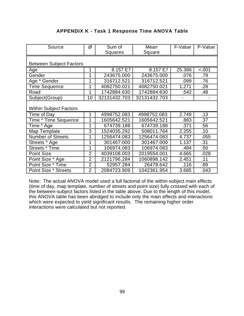
99
APPENDIX K - Task 1 Response Time ANOVA Table
Source df Sum ofSquares
MeanSquare
F-Value P-Value
Between Subject FactorsAge 1 8.157 E7 8.157 E7 25.386 <.001Gender 1 243675.000 243675.000 .076 .79Age * Gender 1 316712.521 316712.521 .099 .76Time Sequence 1 4082750.021 4082750.021 1.271 .28Road 1 1742884.630 1742884.630 .542 .48Subject(Group) 10 32131432.703 32131432.703 - -
Within Subject FactorsTime of Day 1 4998752.083 4998752.083 2.749 .13Time * Time Sequence 1 1605642.521 1605642.521 .883 .37Time * Age 1 674739.188 674739.188 .371 .56Map Template 3 1524035.292 508011.764 2.255 .10Number of Streets 1 1256474.083 1256474.083 4.737 .055Streets * Age 1 301467.000 301467.000 1.137 .31Streets * Time 1 106974.083 106974.083 .484 .50Point Size 2 4039108.003 2019554.001 4.665 .028Point Size * Age 2 2121796.284 1060898.142 2.451 .11Point Size * Time 2 52957.284 26478.642 .116 .89Point Size * Streets 2 2084723.909 1042361.954 3.685 .043
Note: The actual ANOVA model used a full factorial of the within-subject main effects(time of day, map template, number of streets and point size) fully crossed with each ofthe between-subject factors listed in the table above. Due to the length of this model,this ANOVA table has been abridged to include only the main effects and interactionswhich were expected to yield significant results. The remaining higher orderinteractions were calculated but not reported.

100
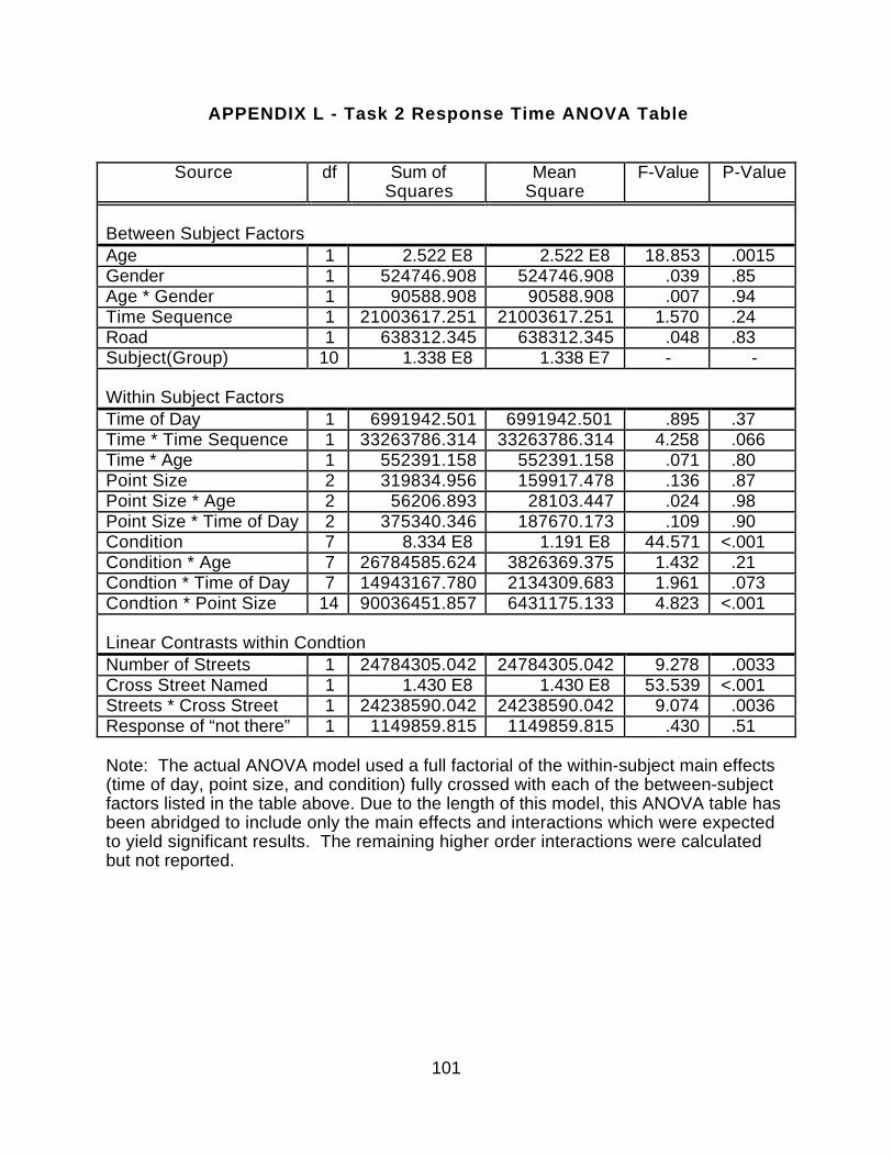
101
APPENDIX L - Task 2 Response Time ANOVA Table
Source df Sum ofSquares
MeanSquare
F-Value P-Value
Between Subject FactorsAge 1 2.522 E8 2.522 E8 18.853 .0015Gender 1 524746.908 524746.908 .039 .85Age * Gender 1 90588.908 90588.908 .007 .94Time Sequence 1 21003617.251 21003617.251 1.570 .24Road 1 638312.345 638312.345 .048 .83Subject(Group) 10 1.338 E8 1.338 E7 - -
Within Subject FactorsTime of Day 1 6991942.501 6991942.501 .895 .37Time * Time Sequence 1 33263786.314 33263786.314 4.258 .066Time * Age 1 552391.158 552391.158 .071 .80Point Size 2 319834.956 159917.478 .136 .87Point Size * Age 2 56206.893 28103.447 .024 .98Point Size * Time of Day 2 375340.346 187670.173 .109 .90Condition 7 8.334 E8 1.191 E8 44.571 <.001Condition * Age 7 26784585.624 3826369.375 1.432 .21Condtion * Time of Day 7 14943167.780 2134309.683 1.961 .073Condtion * Point Size 14 90036451.857 6431175.133 4.823 <.001
Linear Contrasts within CondtionNumber of Streets 1 24784305.042 24784305.042 9.278 .0033Cross Street Named 1 1.430 E8 1.430 E8 53.539 <.001Streets * Cross Street 1 24238590.042 24238590.042 9.074 .0036Response of “not there” 1 1149859.815 1149859.815 .430 .51
Note: The actual ANOVA model used a full factorial of the within-subject main effects(time of day, point size, and condition) fully crossed with each of the between-subjectfactors listed in the table above. Due to the length of this model, this ANOVA table hasbeen abridged to include only the main effects and interactions which were expectedto yield significant results. The remaining higher order interactions were calculatedbut not reported.

102
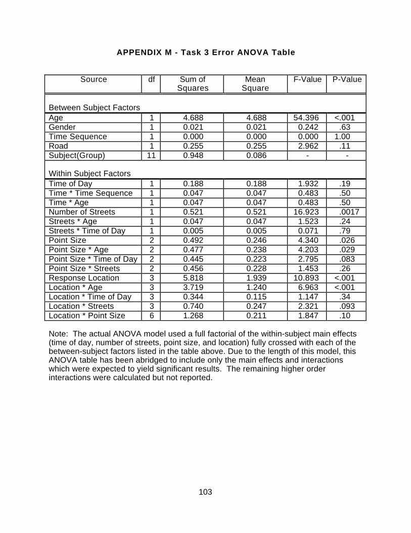
103
APPENDIX M - Task 3 Error ANOVA Table
Source df Sum ofSquares
MeanSquare
F-Value P-Value
Between Subject FactorsAge 1 4.688 4.688 54.396 <.001Gender 1 0.021 0.021 0.242 .63Time Sequence 1 0.000 0.000 0.000 1.00Road 1 0.255 0.255 2.962 .11Subject(Group) 11 0.948 0.086 - -
Within Subject FactorsTime of Day 1 0.188 0.188 1.932 .19Time * Time Sequence 1 0.047 0.047 0.483 .50Time * Age 1 0.047 0.047 0.483 .50Number of Streets 1 0.521 0.521 16.923 .0017Streets * Age 1 0.047 0.047 1.523 .24Streets * Time of Day 1 0.005 0.005 0.071 .79Point Size 2 0.492 0.246 4.340 .026Point Size * Age 2 0.477 0.238 4.203 .029Point Size * Time of Day 2 0.445 0.223 2.795 .083Point Size * Streets 2 0.456 0.228 1.453 .26Response Location 3 5.818 1.939 10.893 <.001Location * Age 3 3.719 1.240 6.963 <.001Location * Time of Day 3 0.344 0.115 1.147 .34Location * Streets 3 0.740 0.247 2.321 .093Location * Point Size 6 1.268 0.211 1.847 .10
Note: The actual ANOVA model used a full factorial of the within-subject main effects(time of day, number of streets, point size, and location) fully crossed with each of thebetween-subject factors listed in the table above. Due to the length of this model, thisANOVA table has been abridged to include only the main effects and interactionswhich were expected to yield significant results. The remaining higher orderinteractions were calculated but not reported.

104
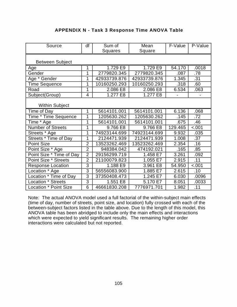
105
APPENDIX N - Task 3 Response Time ANOVA Table
Source df Sum ofSquares
MeanSquare
F-Value P-Value
Between SubjectAge 1 1.729 E9 1.729 E9 54.170 .0018Gender 1 2779820.345 2779820.345 .087 .78Age * Gender 1 42933739.876 42933739.876 1.345 .31Time Sequence 1 10160250.293 10160250.293 .318 .60Road 1 2.086 E8 2.086 E8 6.534 .063Subject(Group) 4 1.277 E8 1.277 E8 - -
Within SubjectTime of Day 1 5614101.001 5614101.001 6.136 .068Time * Time Sequence 1 1205630.262 1205630.262 .145 .72Time * Age 1 5614101.001 5614101.001 .675 .46Number of Streets 1 9.766 E8 9.766 E8 129.465 <.001Streets * Age 1 74923144.699 74923144.699 9.932 .035Streets * Time of Day 1 2124471.939 2124471.939 1.008 .37Point Size 2 13523262.469 13523262.469 2.354 .16Point Size * Age 2 948384.042 474192.021 .165 .85Point Size * Time of Day 2 29156299.719 1.458 E7 3.261 .092Point Size * Streets 2 21100079.823 1.055 E7 2.915 .11Response Location 3 1.188 E9 3.961 E8 54.950 <.001Location * Age 3 56556083.900 1.885 E7 2.615 .10Location * Time of Day 3 37350408.473 1.245 E7 6.030 .0096Location * Streets 3 1.551 E8 5.170 E7 8.051 .0033Location * Point Size 6 46661830.208 7776971.701 1.982 .11
Note: The actual ANOVA model used a full factorial of the within-subject main effects(time of day, number of streets, point size, and location) fully crossed with each of thebetween-subject factors listed in the table above. Due to the length of this model, thisANOVA table has been abridged to include only the main effects and interactionswhich were expected to yield significant results. The remaining higher orderinteractions were calculated but not reported.

106
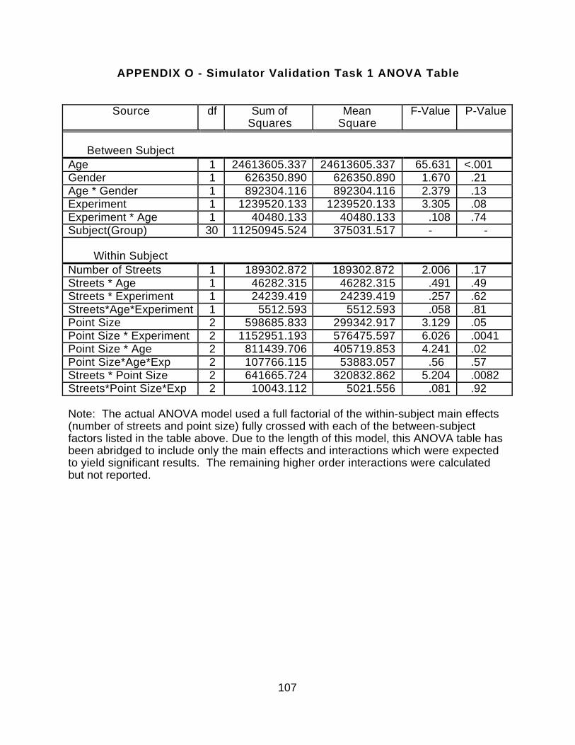
107
APPENDIX O - Simulator Validation Task 1 ANOVA Table
Source df Sum ofSquares
MeanSquare
F-Value P-Value
Between SubjectAge 1 24613605.337 24613605.337 65.631 <.001Gender 1 626350.890 626350.890 1.670 .21Age * Gender 1 892304.116 892304.116 2.379 .13Experiment 1 1239520.133 1239520.133 3.305 .08Experiment * Age 1 40480.133 40480.133 .108 .74Subject(Group) 30 11250945.524 375031.517 - -
Within SubjectNumber of Streets 1 189302.872 189302.872 2.006 .17Streets * Age 1 46282.315 46282.315 .491 .49Streets * Experiment 1 24239.419 24239.419 .257 .62Streets*Age*Experiment 1 5512.593 5512.593 .058 .81Point Size 2 598685.833 299342.917 3.129 .05Point Size * Experiment 2 1152951.193 576475.597 6.026 .0041Point Size * Age 2 811439.706 405719.853 4.241 .02Point Size*Age*Exp 2 107766.115 53883.057 .56 .57Streets * Point Size 2 641665.724 320832.862 5.204 .0082Streets*Point Size*Exp 2 10043.112 5021.556 .081 .92
Note: The actual ANOVA model used a full factorial of the within-subject main effects(number of streets and point size) fully crossed with each of the between-subjectfactors listed in the table above. Due to the length of this model, this ANOVA table hasbeen abridged to include only the main effects and interactions which were expectedto yield significant results. The remaining higher order interactions were calculatedbut not reported.

108

109
APPENDIX P - Comparison of Display Positions
4"
15"
Simulator
1985 Chrysler Laser
1"
20"
On-the-Road
1992 Ford Taurus Wagon
Note: All measurements were taken from the steering wheel adjusted in mid-position.

110
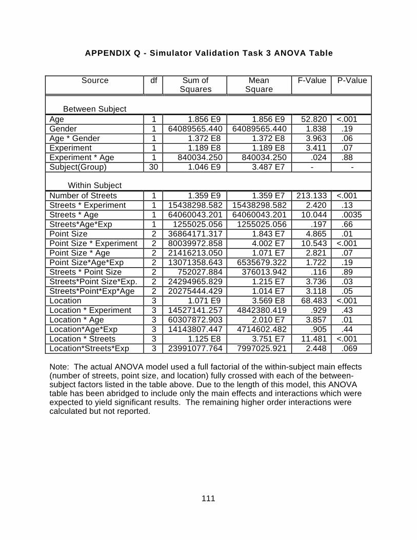
111
APPENDIX Q - Simulator Validation Task 3 ANOVA Table
Source df Sum ofSquares
MeanSquare
F-Value P-Value
Between SubjectAge 1 1.856 E9 1.856 E9 52.820 <.001Gender 1 64089565.440 64089565.440 1.838 .19Age * Gender 1 1.372 E8 1.372 E8 3.963 .06Experiment 1 1.189 E8 1.189 E8 3.411 .07Experiment * Age 1 840034.250 840034.250 .024 .88Subject(Group) 30 1.046 E9 3.487 E7 - -
Within SubjectNumber of Streets 1 1.359 E9 1.359 E7 213.133 <.001Streets * Experiment 1 15438298.582 15438298.582 2.420 .13Streets * Age 1 64060043.201 64060043.201 10.044 .0035Streets*Age*Exp 1 1255025.056 1255025.056 .197 .66Point Size 2 36864171.317 1.843 E7 4.865 .01Point Size * Experiment 2 80039972.858 4.002 E7 10.543 <.001Point Size * Age 2 21416213.050 1.071 E7 2.821 .07Point Size*Age*Exp 2 13071358.643 6535679.322 1.722 .19Streets * Point Size 2 752027.884 376013.942 .116 .89Streets*Point Size*Exp. 2 24294965.829 1.215 E7 3.736 .03Streets*Point*Exp*Age 2 20275444.429 1.014 E7 3.118 .05Location 3 1.071 E9 3.569 E8 68.483 <.001Location * Experiment 3 14527141.257 4842380.419 .929 .43Location * Age 3 60307872.903 2.010 E7 3.857 .01Location*Age*Exp 3 14143807.447 4714602.482 .905 .44Location * Streets 3 1.125 E8 3.751 E7 11.481 <.001Location*Streets*Exp 3 23991077.764 7997025.921 2.448 .069
Note: The actual ANOVA model used a full factorial of the within-subject main effects(number of streets, point size, and location) fully crossed with each of the between-subject factors listed in the table above. Due to the length of this model, this ANOVAtable has been abridged to include only the main effects and interactions which wereexpected to yield significant results. The remaining higher order interactions werecalculated but not reported.