Map-ReducePractice

Lecture 03.02

By Marina BarskyWinter 2016, University of Toronto

Big-data processing

• Scalability of algorithms

• Inherently parallelizable tasks

• Distributed file system

• Map-reduce computation

• Practice

Practice

Example 1: what does it do

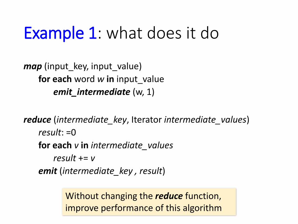
map (input_key, input_value)

for each word w in input_value

emit_intermediate (w, 1)

reduce (intermediate_key, Iterator intermediate_values)

result: =0

for each v in intermediate_values

result += v

emit (intermediate_key , result)

Without changing the reduce function, improve performance of this algorithm

Refinement: Combiners

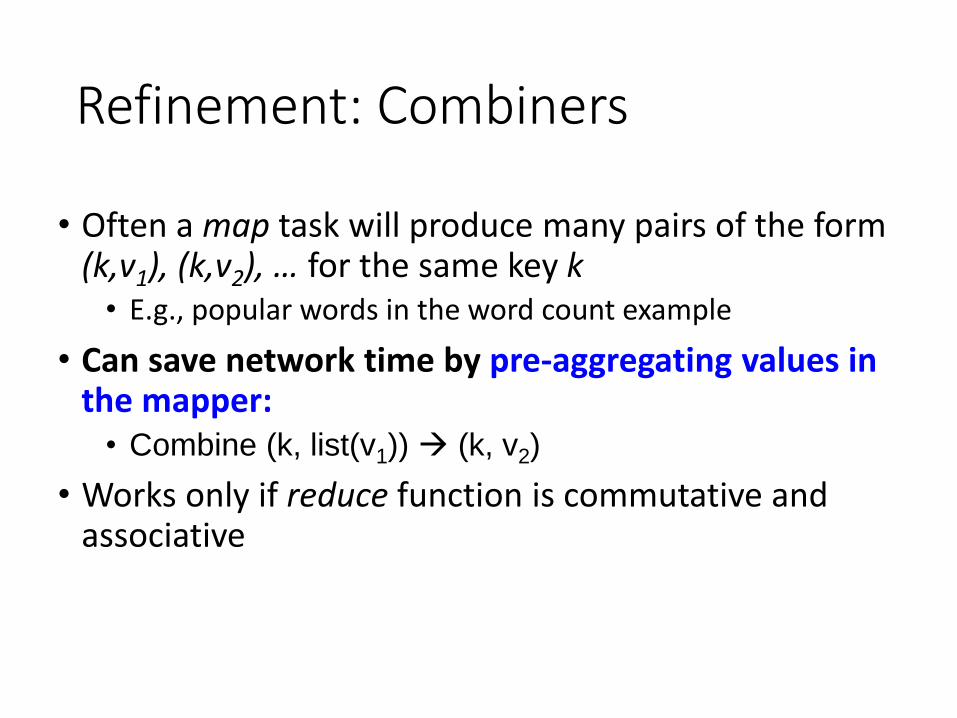
• Often a map task will produce many pairs of the form (k,v1), (k,v2), … for the same key k• E.g., popular words in the word count example

• Can save network time by pre-aggregating values in the mapper:• Combine (k, list(v1)) (k, v2)

• Works only if reduce function is commutative and associative

Refinement: Combiners

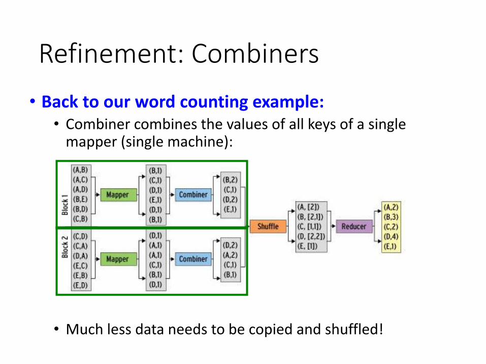
• Back to our word counting example:• Combiner combines the values of all keys of a single

mapper (single machine):

• Much less data needs to be copied and shuffled!

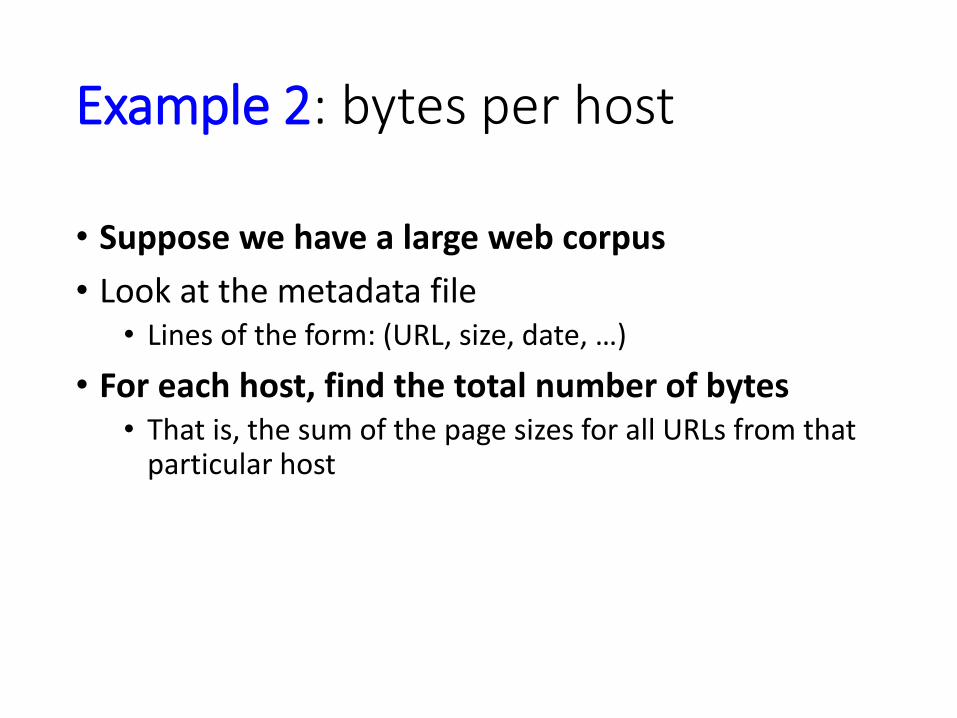
Example 2: bytes per host

• Suppose we have a large web corpus

• Look at the metadata file• Lines of the form: (URL, size, date, …)

• For each host, find the total number of bytes• That is, the sum of the page sizes for all URLs from that

particular host

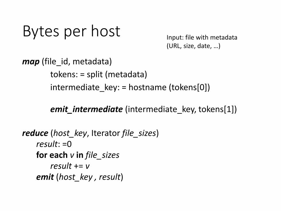
Bytes per host

map (file_id, metadata)

tokens: = split (metadata)

intermediate_key: = hostname (tokens[0])

emit_intermediate (intermediate_key, tokens[1])

reduce (host_key, Iterator file_sizes)result: =0for each v in file_sizes

result += vemit (host_key , result)

Input: file with metadata(URL, size, date, …)

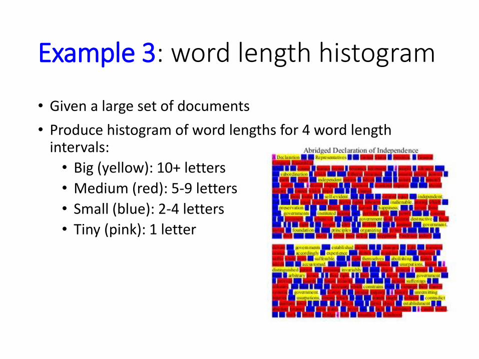
Example 3: word length histogram

• Given a large set of documents

• Produce histogram of word lengths for 4 word length intervals:

• Big (yellow): 10+ letters

• Medium (red): 5-9 letters

• Small (blue): 2-4 letters

• Tiny (pink): 1 letter

Word length histogram: input and output • Input: a set of documents

• Output:

• (big, 62)

• (medium, 124)

• (small, 76)

• (tiny, 12)

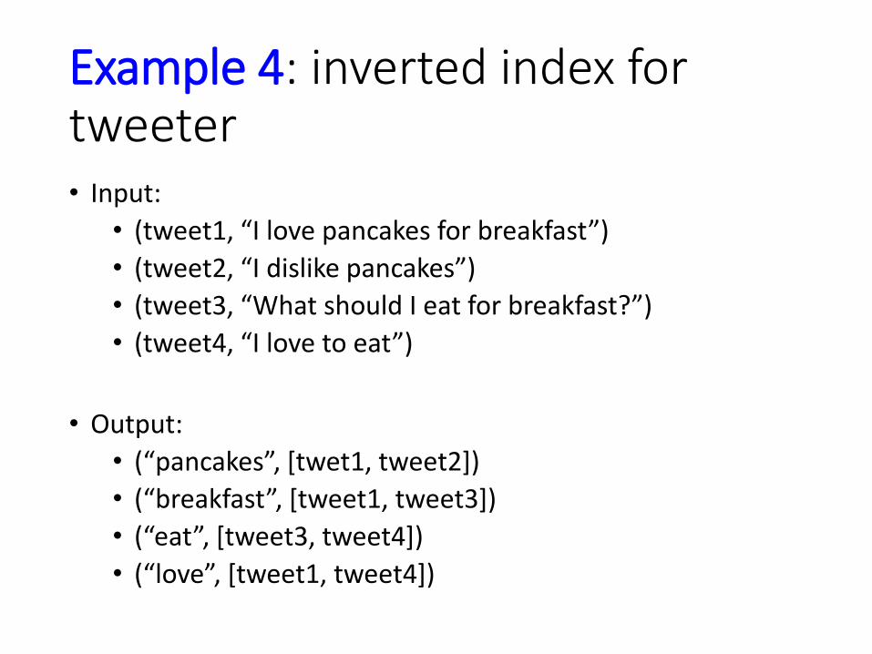
Example 4: inverted index for tweeter• Input:

• (tweet1, “I love pancakes for breakfast”)

• (tweet2, “I dislike pancakes”)

• (tweet3, “What should I eat for breakfast?”)

• (tweet4, “I love to eat”)

• Output:

• (“pancakes”, [twet1, tweet2])

• (“breakfast”, [tweet1, tweet3])

• (“eat”, [tweet3, tweet4])

• (“love”, [tweet1, tweet4])

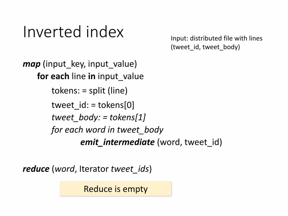
Inverted index

map (input_key, input_value)

for each line in input_value

tokens: = split (line)

tweet_id: = tokens[0]

tweet_body: = tokens[1]

for each word in tweet_body

emit_intermediate (word, tweet_id)

reduce (word, Iterator tweet_ids)

Input: distributed file with lines(tweet_id, tweet_body)

Reduce is empty

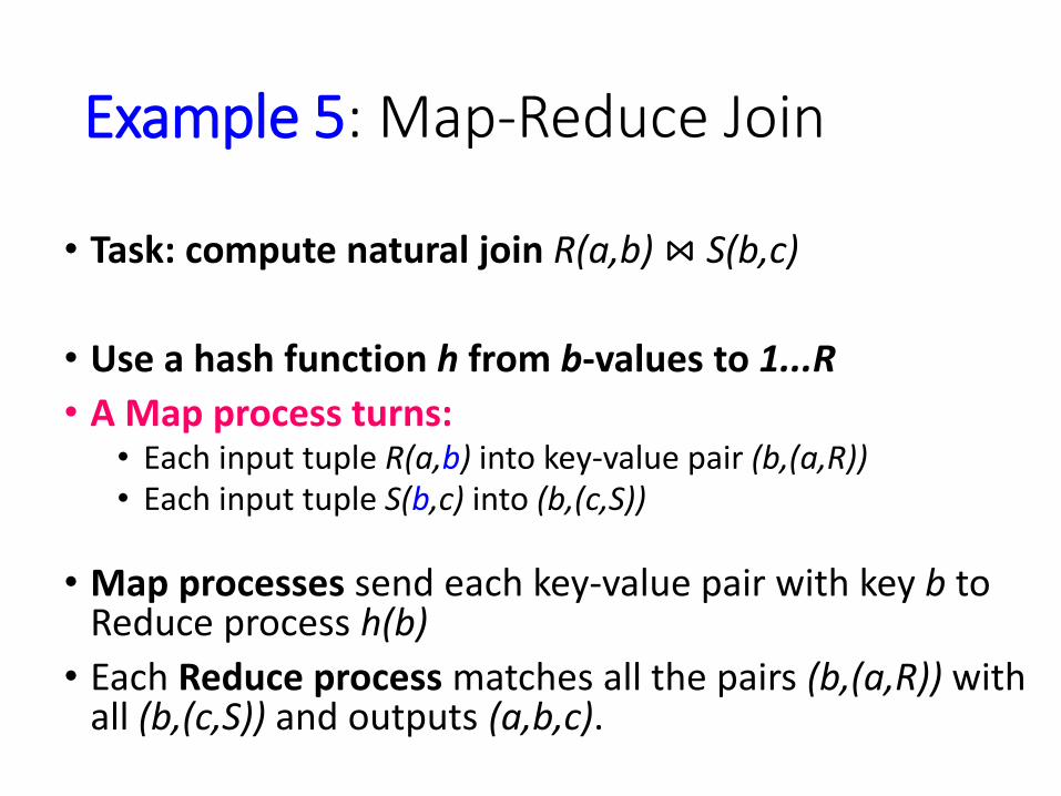
Example 5: Map-Reduce Join

• Task: compute natural join R(a,b) ⋈ S(b,c)

• Use a hash function h from b-values to 1...R

• A Map process turns:• Each input tuple R(a,b) into key-value pair (b,(a,R))• Each input tuple S(b,c) into (b,(c,S))

• Map processes send each key-value pair with key b to Reduce process h(b)

• Each Reduce process matches all the pairs (b,(a,R)) with all (b,(c,S)) and outputs (a,b,c).

Join: step-by-step

SIN Department

111111 Accounting

111111 Sales

333333 Marketing

Name SIN

Mary 111111

John 333333

Employee AssignedDepartment

Name SIN Department

Mary 111111 Accounting

Mary 111111 Sales

John 333333 Marketing

Employee ⋈AssignedDepartment

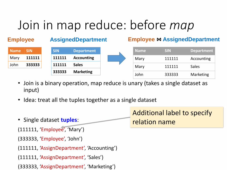
Join in map reduce: before map

• Join is a binary operation, map reduce is unary (takes a single dataset as input)

• Idea: treat all the tuples together as a single dataset

• Single dataset tuples:

(111111, ‘Employee’, ‘Mary’)

(333333, ‘Employee’, ‘John’)

(111111, ‘AssignDepartment’, ‘Accounting’)

(111111, ‘AssignDepartment’, ‘Sales’)

(333333, ‘AssignDepartment’, ‘Marketing’)

SIN Department

111111 Accounting

111111 Sales

333333 Marketing

Name SIN

Mary 111111

John 333333

Employee AssignedDepartment

Name SIN Department

Mary 111111 Accounting

Mary 111111 Sales

John 333333 Marketing

Employee ⋈AssignedDepartment

Additional label to specify relation name

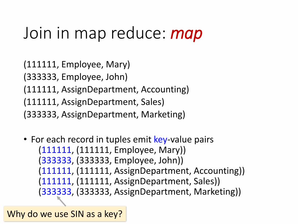
Join in map reduce: map

(111111, Employee, Mary)

(333333, Employee, John)

(111111, AssignDepartment, Accounting)

(111111, AssignDepartment, Sales)

(333333, AssignDepartment, Marketing)

• For each record in tuples emit key-value pairs(111111, (111111, Employee, Mary))(333333, (333333, Employee, John))(111111, (111111, AssignDepartment, Accounting))(111111, (111111, AssignDepartment, Sales))(333333, (333333, AssignDepartment, Marketing))

Why do we use SIN as a key?

Join in map reduce: magic shuffle phase

• Everything with the same key is lumped together on a single reducer

(111111, [(111111, Employee, Mary), (111111, AssignDepartment, Accounting), (111111, AssignDepartment, Sales)] )

(333333, [(333333, Employee, John), (333333, AssignDepartment, Marketing)]

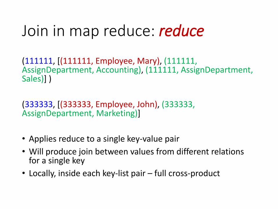
Join in map reduce: reduce

(111111, [(111111, Employee, Mary), (111111, AssignDepartment, Accounting), (111111, AssignDepartment, Sales)] )

(333333, [(333333, Employee, John), (333333, AssignDepartment, Marketing)]

• Applies reduce to a single key-value pair

• Will produce join between values from different relations for a single key

• Locally, inside each key-list pair – full cross-product

Join in map reducemap (relation_name, (join_attr_name, relation))

for each tuple t in relation

emit_intermediate (t[join_attr_name], (relation_name, t))

reduce (join_attr_val, Iterator tuples_to_join)

emp_tuples: = []

dept_tuples: = []

for each v in tuples_to_join

if (v [0] = “Employee”)

emp_tuples += v[1]

else

dept_tuples += v[1]

for each e in emp_tuples

for each d in dept_tuples

emit (join_attr_val , (e,d))

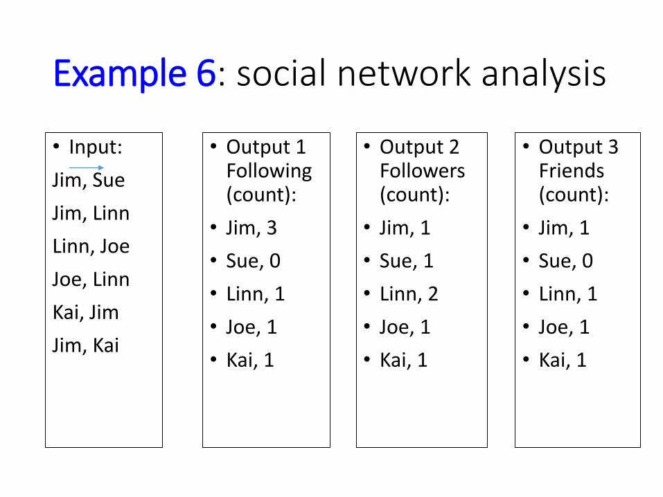
Example 6: social network analysis

• Input:

Jim, Sue

Jim, Linn

Linn, Joe

Joe, Linn

Kai, Jim

Jim, Kai

• Output 1 Following (count):

• Jim, 3

• Sue, 0

• Linn, 1

• Joe, 1

• Kai, 1

• Output 2 Followers (count):

• Jim, 1

• Sue, 1

• Linn, 2

• Joe, 1

• Kai, 1

• Output 3 Friends (count):

• Jim, 1

• Sue, 0

• Linn, 1

• Joe, 1

• Kai, 1

Followers: list of followers for each usermap (file_name, edges)

for each edge in edges

emit_intermediate (edge[1], edge[0])

reduce (user_id, Iterator followers)

Example 7: Max integer

• Design MapReduce algorithm to take a very large file of integers and produce as output:

the largest integer.

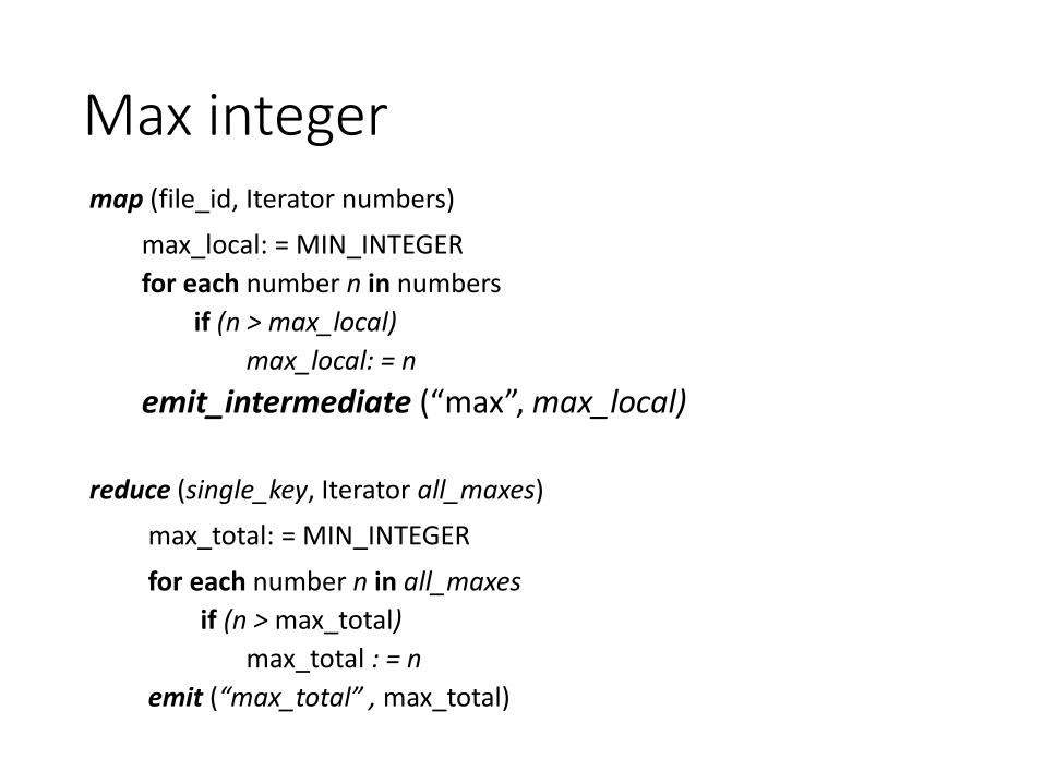
Max integermap (file_id, Iterator numbers)

max_local: = MIN_INTEGER

for each number n in numbers

if (n > max_local)

max_local: = n

emit_intermediate (“max”, max_local)

reduce (single_key, Iterator all_maxes)

max_total: = MIN_INTEGER

for each number n in all_maxes

if (n > max_total)

max_total : = n

emit (“max_total” , max_total)

Example 8: Duplicate elimination

• Design MapReduce algorithm to take a very large file of integers and produce as output:

the same set of integers, but with each integer appearing only once.

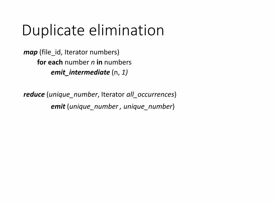
Duplicate eliminationmap (file_id, Iterator numbers)

for each number n in numbers

emit_intermediate (n, 1)

reduce (unique_number, Iterator all_occurrences)

emit (unique_number , unique_number)

Example 9: Union, intersection, differenceSet Union:

• The Map Function: Turns each input tuple t into a key-value pair (t, t).

• The Reduce Function: Associated with each key t there will be either one or two values. Produce output (t, t) in either case.

Example 9: Union, intersection, differenceIntersection:

• To compute the intersection, we can use the same Map function.

• However, the Reduce function must produce a tuple only if both relations have the tuple. If the key t has a list of two values [t, t] associated with it, then the Reduce task for t should produce (t, t). However, if the value-list associated with key t is just [t], then one of R and S is missing t, so we don’t want to produce a tuple for the intersection.

• The Map Function: Turn each tuple t into a key-value pair (t, t).

• The Reduce Function: If key t has value list [t, t], then produce (t, t). Otherwise, produce nothing.

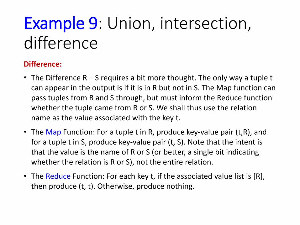
Example 9: Union, intersection, differenceDifference:

• The Difference R − S requires a bit more thought. The only way a tuple t can appear in the output is if it is in R but not in S. The Map function can pass tuples from R and S through, but must inform the Reduce function whether the tuple came from R or S. We shall thus use the relation name as the value associated with the key t.

• The Map Function: For a tuple t in R, produce key-value pair (t,R), and for a tuple t in S, produce key-value pair (t, S). Note that the intent is that the value is the name of R or S (or better, a single bit indicating whether the relation is R or S), not the entire relation.

• The Reduce Function: For each key t, if the associated value list is [R], then produce (t, t). Otherwise, produce nothing.

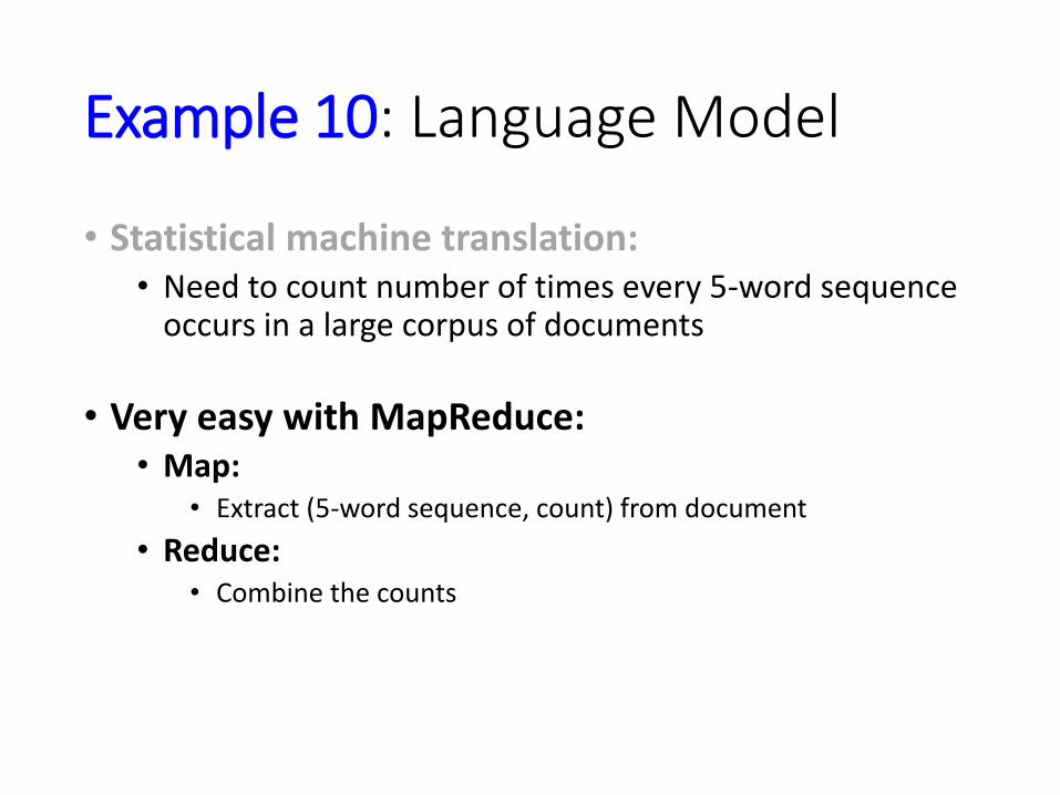
Example 10: Language Model

• Statistical machine translation:• Need to count number of times every 5-word sequence

occurs in a large corpus of documents

• Very easy with MapReduce:• Map:

• Extract (5-word sequence, count) from document

• Reduce: • Combine the counts

Example 11: matrix-vector multiplication

• Originally, map-reduce was designed for fast computation of web page ranks using PageRank algorithm

How to rank web pages

It seems that:

• a problem is the self-referential nature of this definition;

• if we follow this line of reasoning, we might find that the importance of a web page depends on itself!

Definition: A webpage is important if many important pages link to it.

Modeling the web

• What can we speculate about the relative importance of pages in each of these graphs, solely from the structure of the links (which is anyways the only information at hand)?

B

C

D

B

C

D

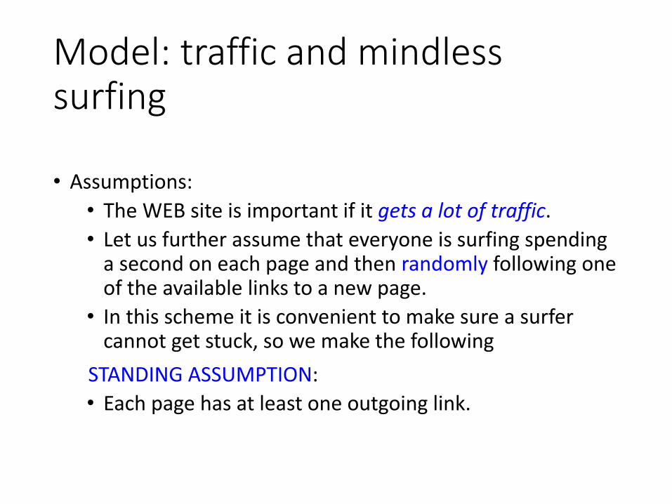
Model: traffic and mindless surfing

• Assumptions:

• The WEB site is important if it gets a lot of traffic.

• Let us further assume that everyone is surfing spending a second on each page and then randomly following one of the available links to a new page.

• In this scheme it is convenient to make sure a surfer cannot get stuck, so we make the following

STANDING ASSUMPTION:

• Each page has at least one outgoing link.

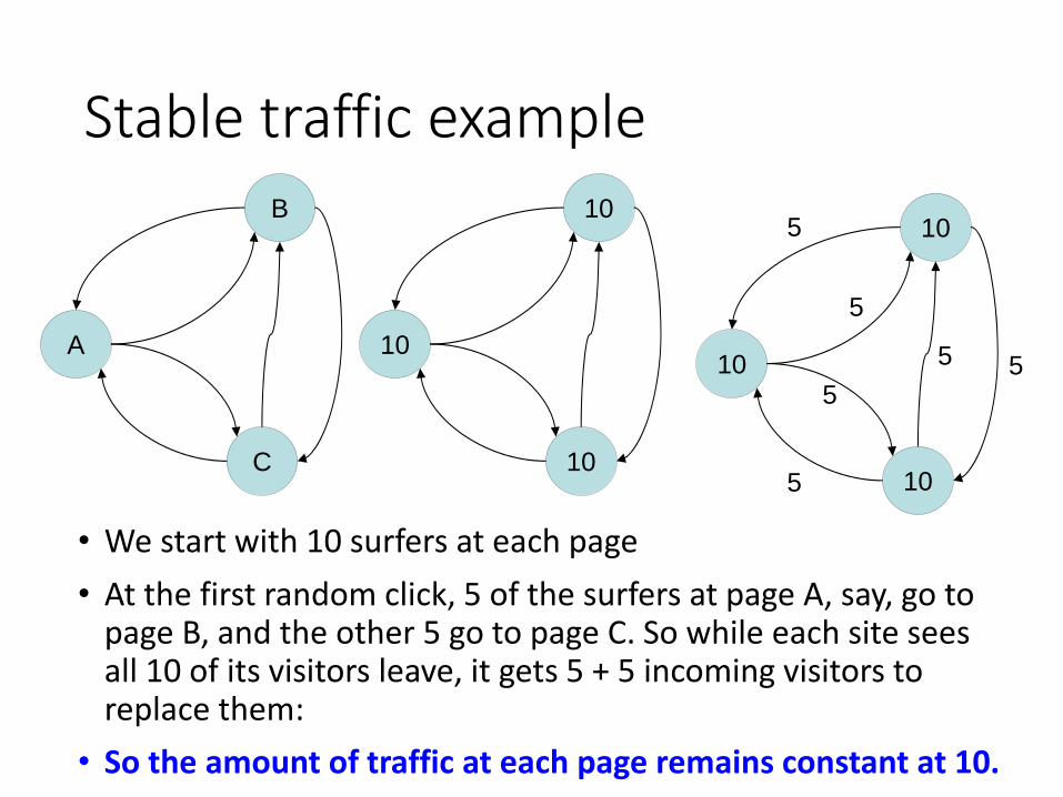
Stable traffic example

• We start with 10 surfers at each page

• At the first random click, 5 of the surfers at page A, say, go to page B, and the other 5 go to page C. So while each site sees all 10 of its visitors leave, it gets 5 + 5 incoming visitors to replace them:

• So the amount of traffic at each page remains constant at 10.

B

A

C

10

10

10

10

10

10

5

5

5

5

5 5

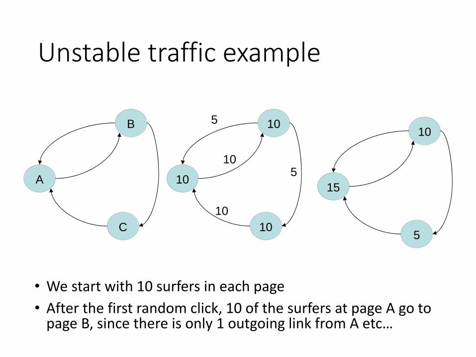
Unstable traffic example

• We start with 10 surfers in each page

• After the first random click, 10 of the surfers at page A go to page B, since there is only 1 outgoing link from A etc…

B

A

C

10

10

10

10

15

5

5

5

10

10

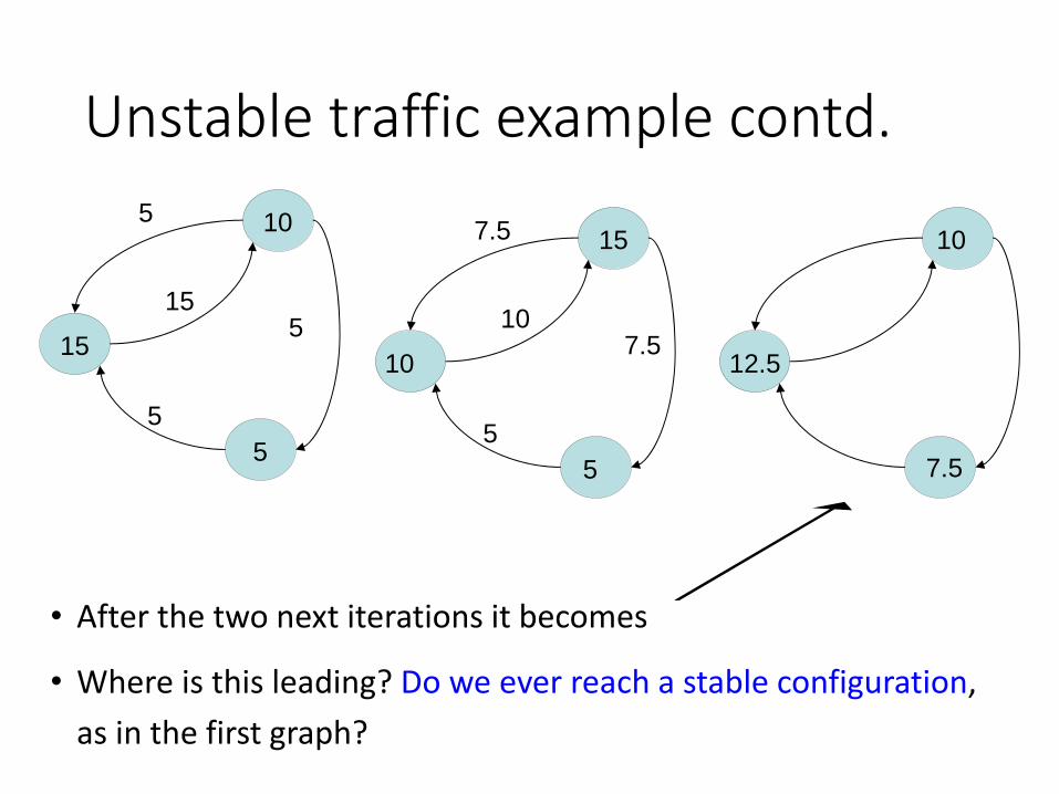
Unstable traffic example contd.

• After the two next iterations it becomes

• Where is this leading? Do we ever reach a stable configuration,

as in the first graph?

10

15

5

5

5

5

15

15

10

5

7.5

7.5

5

10

10

12.5

7.5

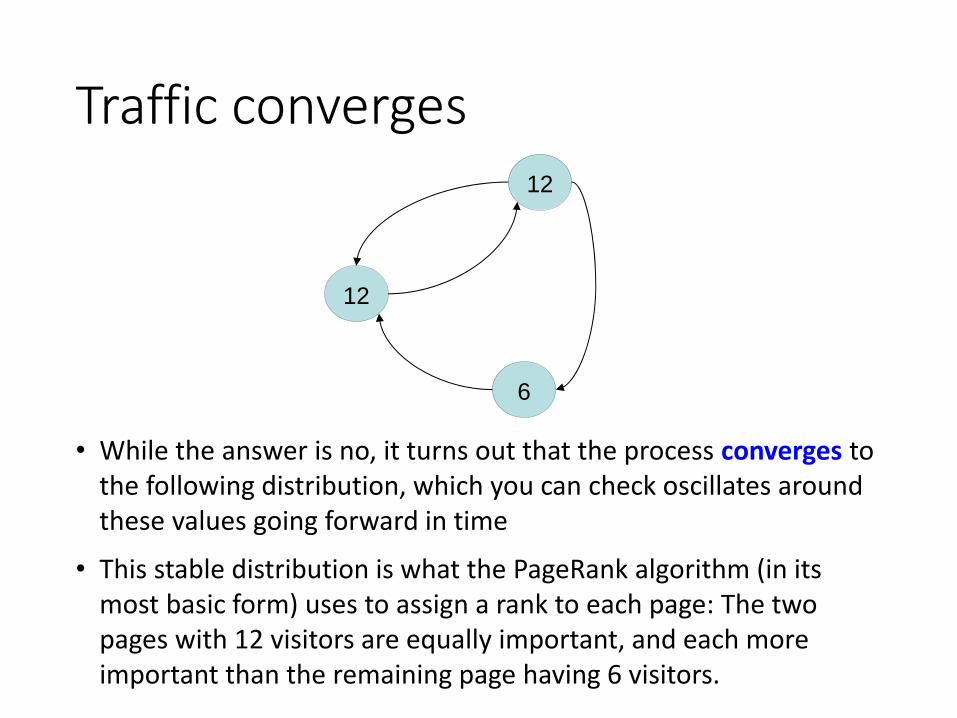
Traffic converges

• While the answer is no, it turns out that the process converges to the following distribution, which you can check oscillates around these values going forward in time

• This stable distribution is what the PageRank algorithm (in its most basic form) uses to assign a rank to each page: The two pages with 12 visitors are equally important, and each more important than the remaining page having 6 visitors.

12

12

6

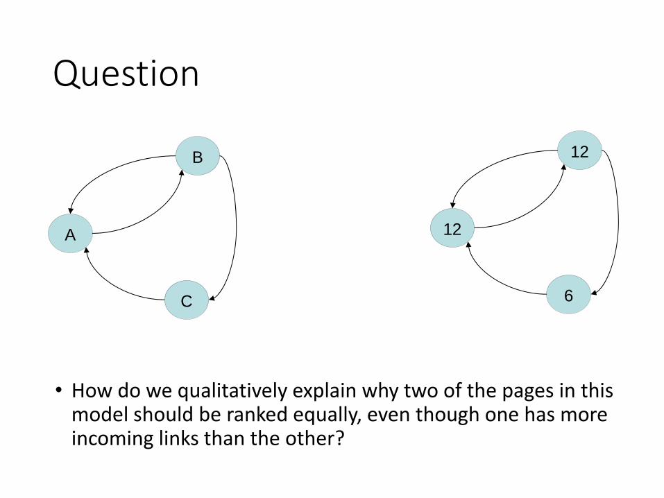
Question

• How do we qualitatively explain why two of the pages in this model should be ranked equally, even though one has more incoming links than the other?

12

12

6

B

A

C

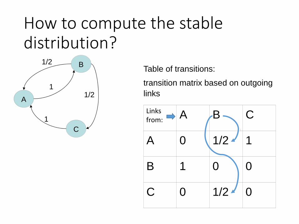
How to compute the stable distribution?

B

A

C

1/2

1/2

1

1

A B C

A 0 1/2 1

B 1 0 0

C 0 1/2 0

Table of transitions:

transition matrix based on outgoing

links

Links from:

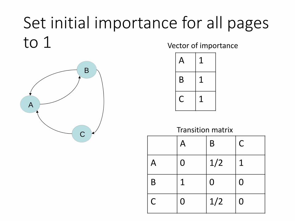
Set initial importance for all pages to 1

A B C

A 0 1/2 1

B 1 0 0

C 0 1/2 0

B

A

CTransition matrix

Vector of importance

A 1

B 1

C 1

Iteration 1

A B C

A 0 1/2 1

B 1 0 0

C 0 1/2 0

Transition matrix

Current Vector of importance

A 1

B 1

C 1

A 1*1/2 + 1*1 =1.5

B 1*1 = 1

C 1*1/2 = 1/2

New Vector of importance

From B From C

Find new importance based on number of incoming visitors and their rank

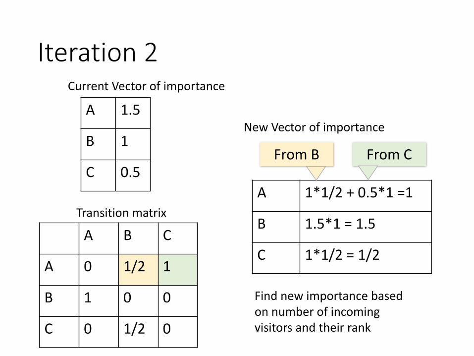
Iteration 2

A B C

A 0 1/2 1

B 1 0 0

C 0 1/2 0

Transition matrix

Current Vector of importance

A 1.5

B 1

C 0.5

A 1*1/2 + 0.5*1 =1

B 1.5*1 = 1.5

C 1*1/2 = 1/2

New Vector of importance

From B From C

Find new importance based on number of incoming visitors and their rank

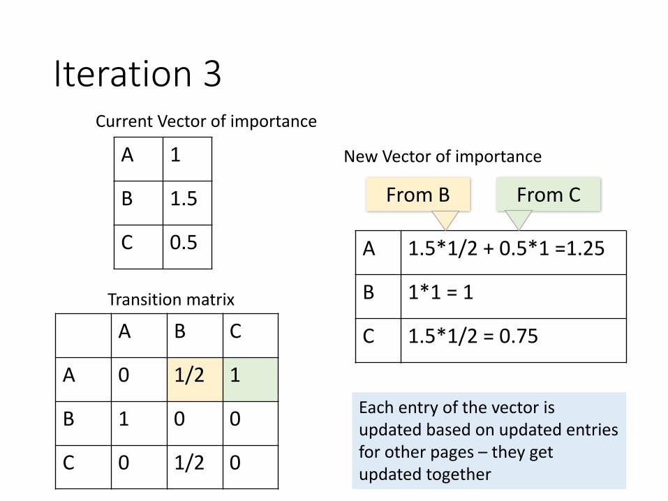
Iteration 3

A B C

A 0 1/2 1

B 1 0 0

C 0 1/2 0

Transition matrix

Current Vector of importance

A 1

B 1.5

C 0.5 A 1.5*1/2 + 0.5*1 =1.25

B 1*1 = 1

C 1.5*1/2 = 0.75

New Vector of importance

From B From C

Each entry of the vector is updated based on updated entries for other pages – they get updated together

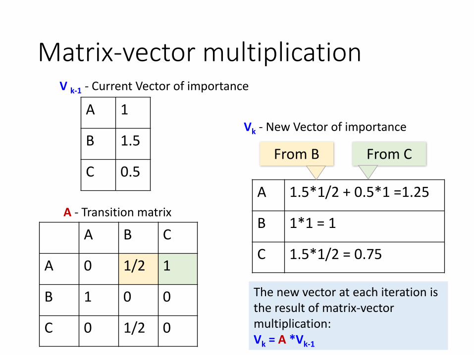
Matrix-vector multiplication

A B C

A 0 1/2 1

B 1 0 0

C 0 1/2 0

A - Transition matrix

V k-1 - Current Vector of importance

A 1

B 1.5

C 0.5

A 1.5*1/2 + 0.5*1 =1.25

B 1*1 = 1

C 1.5*1/2 = 0.75

Vk - New Vector of importance

From B From C

The new vector at each iteration is the result of matrix-vector multiplication:Vk = A *Vk-1

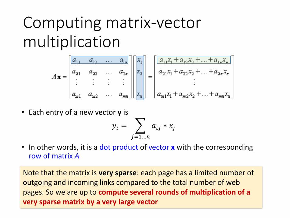
Computing matrix-vector multiplication

• Each entry of a new vector y is

𝑦𝑖 =

𝑗=1…𝑛

𝑎𝑖𝑗 ∗ 𝑥𝑗

• In other words, it is a dot product of vector x with the corresponding row of matrix A

Note that the matrix is very sparse: each page has a limited number of outgoing and incoming links compared to the total number of web pages. So we are up to compute several rounds of multiplication of a very sparse matrix by a very large vector

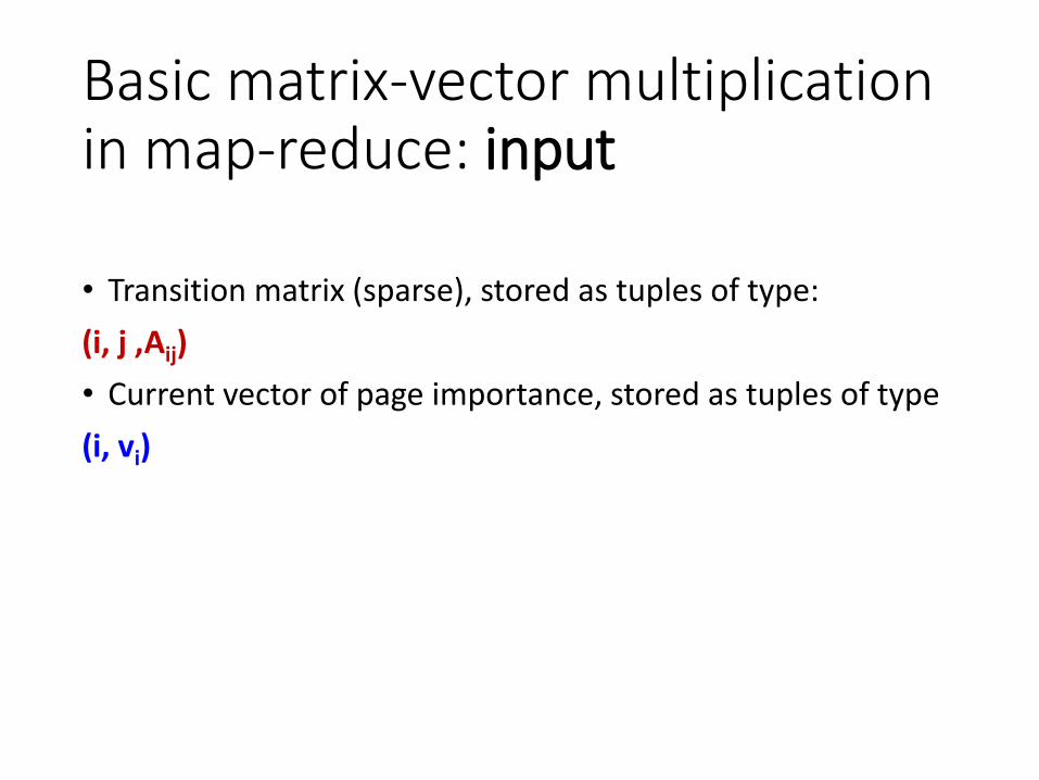
Basic matrix-vector multiplication in map-reduce: input

• Transition matrix (sparse), stored as tuples of type:

(i, j ,Aij)

• Current vector of page importance, stored as tuples of type

(i, vi)

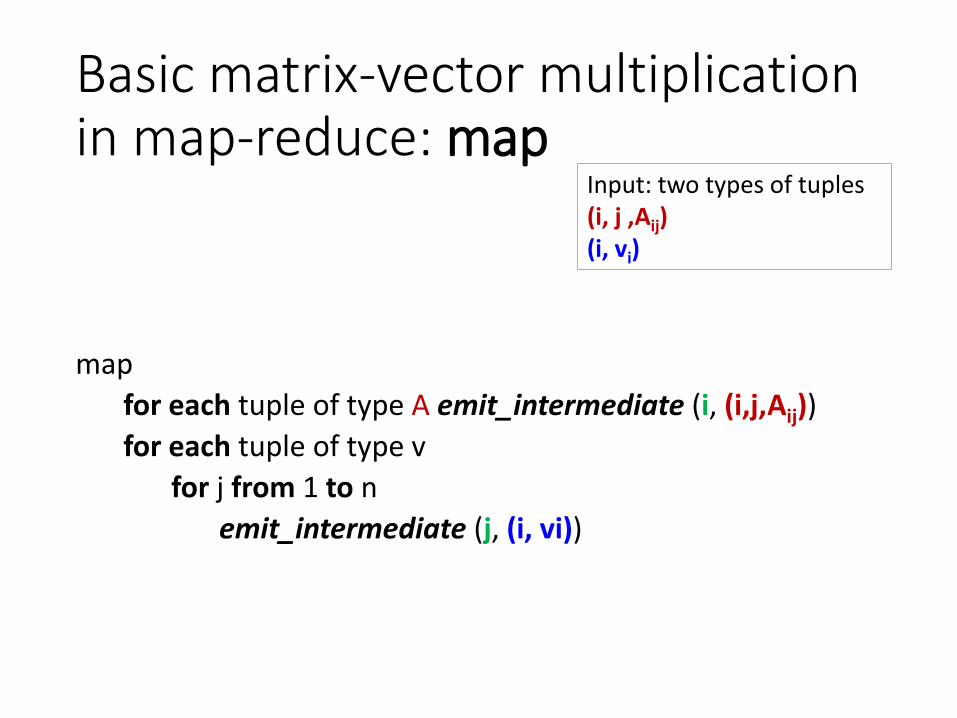
Basic matrix-vector multiplication in map-reduce: map

map

for each tuple of type A emit_intermediate (i, (i,j,Aij))

for each tuple of type v

for j from 1 to n

emit_intermediate (j, (i, vi))

Input: two types of tuples(i, j ,Aij)(i, vi)

Step-by-step example: input

• Tuples of type A:

(1,2,1/2)

(1,3,1)

(2,1,1)

(3,2,1/2)

• Tuples of type v:

(1,1)

(2,1)

(3,1)

A B C

A 0 1/2 1

B 1 0 0

C 0 1/2 0

A 1

B 1

C 1

Step-by-step example: output of map • Output of type A:

(1, (1,2,1/2))

(1, (1,3,1))

(2, (2,1,1))

(3, (3,2,1/2))

• Output of type v:

(1, (1,1))

(2, (1,1))

(3, (1,1))

(1, (2,1))

(2, (2,1))

(3, (2,1))

(1, (3,1))

(2, (3,1))

(3, (3,1))

• Tuples of type A:

(1,2,1/2)

(1,3,1)

(2,1,1)

(3,2,1/2)

• Tuples of type v:

(1,1)

(2,1)

(3,1)

row col val

row val

Step-by-step example: after shuffle

• At each reducer:

• (1, [(1,2,1/2), (1,3,1), (1,1), (2,1), (3,1)])

• (2, [(2,1,1), (1,1), (2,1), (3,1)])

• (3, [(3,2,1/2), (1,1), (2,1), (3,1)])

• Output of type A:

(1, (1,2,1/2))

(1, (1,3,1))

(2, (2,1,1))

(3, (3,2,1/2))

• Output of type v:

(1, (1,1))

(2, (1,1))

(3, (1,1))

(1, (2,1))

(2, (2,1))

(3, (2,1))

(1, (3,1))

(2, (3,1))

(3, (3,1))

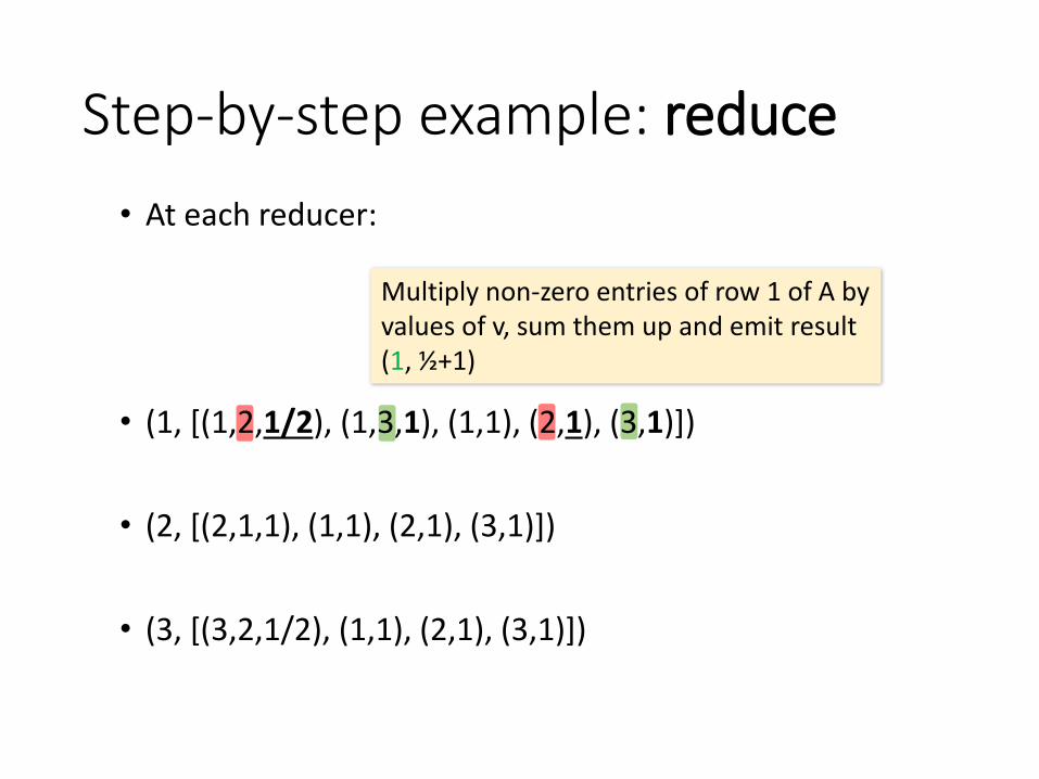
Step-by-step example: reduce

• At each reducer:

• (1, [(1,2,1/2), (1,3,1), (1,1), (2,1), (3,1)])

• (2, [(2,1,1), (1,1), (2,1), (3,1)])

• (3, [(3,2,1/2), (1,1), (2,1), (3,1)])

Multiply non-zero entries of row 1 of A by values of v, sum them up and emit result (1, ½+1)

Basic matrix-vector multiplication in map-reduce: reduce

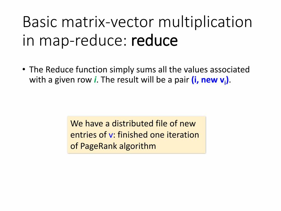
• The Reduce function simply sums all the values associated with a given row i. The result will be a pair (i, new vi).

We have a distributed file of new entries of v: finished one iteration of PageRank algorithm

Basic matrix-vector multiplication: limitations

• It seems that the vector of current ranks (which can be very large) is required by all reducers. This may lead to a very costly network traffic

• To overcome this, we can partition vector v and matrix A, and process each partition on a separate reducer, but we may require more iterations of map-reduce

Partitioned Matrix-Vector multiplication: main idea

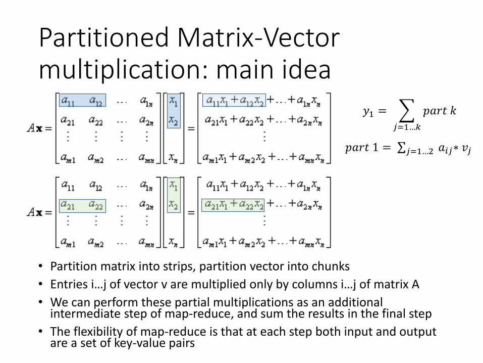
• Partition matrix into strips, partition vector into chunks

• Entries i…j of vector v are multiplied only by columns i…j of matrix A

• We can perform these partial multiplications as an additional intermediate step of map-reduce, and sum the results in the final step

• The flexibility of map-reduce is that at each step both input and output are a set of key-value pairs

𝑝𝑎𝑟𝑡 1 = σ𝑗=1…2 𝑎𝑖𝑗∗ 𝑣𝑗

𝑦1 =

𝑗=1…𝑘

𝑝𝑎𝑟𝑡 𝑘

Cost Measures for Algorithms

In MapReduce we quantify the cost of an algorithm using

1. Communication cost = total I/O of all processes

2. Elapsed communication cost = max of I/O along any path

3. (Elapsed) computation cost analogous, but count only max running time of a single process

Note that here the big-O notation is not the most useful

(adding more machines is always an option)

Example: Cost Measures

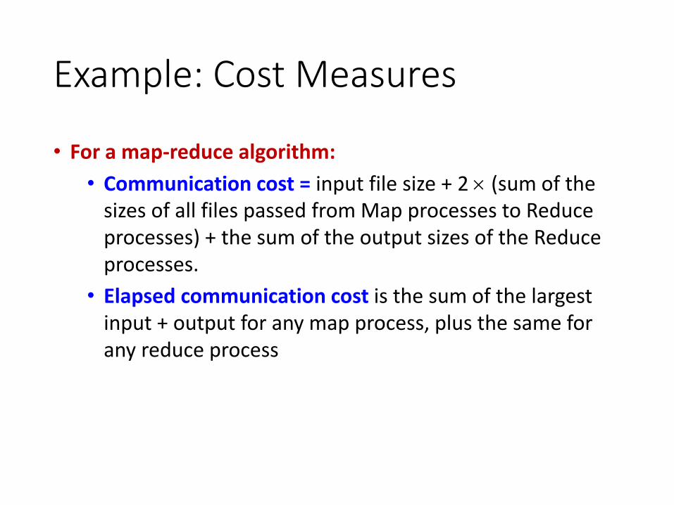
• For a map-reduce algorithm:

• Communication cost = input file size + 2 (sum of the sizes of all files passed from Map processes to Reduce processes) + the sum of the output sizes of the Reduce processes.

• Elapsed communication cost is the sum of the largest input + output for any map process, plus the same for any reduce process

What Cost Measures Mean

• Either the I/O (communication) or processing (computation) cost dominates

• Ignore one or the other

• Total cost tells what you pay in rent from your friendly neighborhood cloud

• Elapsed cost is wall-clock time using parallelism

Implementations

• Google

• Not available outside Google

• Hadoop

• An open-source implementation in Java

• Uses HDFS for stable storage

• Download: http://lucene.apache.org/hadoop/

• Aster Data

• Cluster-optimized SQL Database that also implements MapReduce

Cloud Computing

• Ability to rent computing by the hour

• Additional services e.g., persistent storage

• Amazon’s “Elastic Compute Cloud” (EC2)

• Aster Data and Hadoop can both be run on EC2

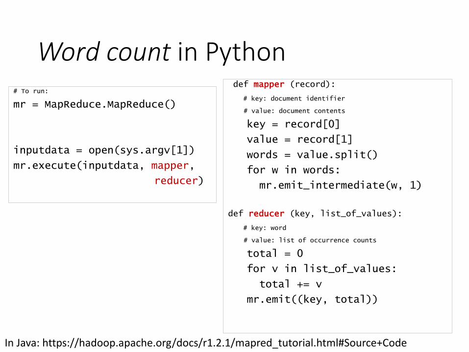
Word count in Pythondef mapper (record):

# key: document identifier

# value: document contents

key = record[0]

value = record[1]

words = value.split()

for w in words:

mr.emit_intermediate(w, 1)

def reducer (key, list_of_values):

# key: word

# value: list of occurrence counts

total = 0

for v in list_of_values:

total += v

mr.emit((key, total))

# To run:

mr = MapReduce.MapReduce()

inputdata = open(sys.argv[1])

mr.execute(inputdata, mapper,

reducer)

In Java: https://hadoop.apache.org/docs/r1.2.1/mapred_tutorial.html#Source+Code

Summary

• Learned how to scale out processing of large inputs

• Map-reduce framework allows to implement only 2

functions and the system takes care of distributing

computations across multiple machines

• Memory footprint is small. Need to care about the size of

intermediate outputs – sending them across network may

dominate the cost

• We can perform relational operations in map reduce, if the

relations are too big to be processed on a single machine

Scalability of parallel architectures

D. J. DeWitt, J. Gray, "Parallel Database Systems: the Future of High Performance Database Systems", ACM Communications, vol. 35(6), 85-98, June 1992.

…

Logical multi-processor database designs

interconnect

…

interconnect

interconnect

Shared nothing Shared disk

…

=disk =memory =processor

Shared memory

Scalability of parallel architectures

…

Logical multi-processor database designs

interconnect

…

interconnect

interconnect

Shared nothing Shared disk

…

=disk =memory =processor

Shared memory

Only shared nothing architecture truly scales, others reach the bottleneck of accessing the same data by multiple processors

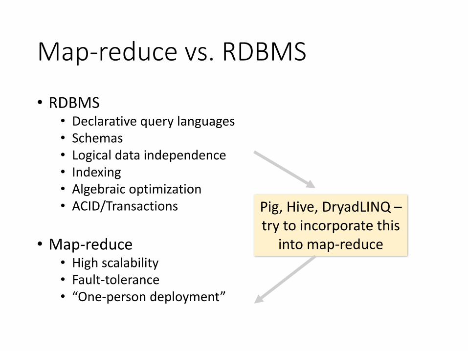
Map-reduce vs. RDBMS

• RDBMS• Declarative query languages• Schemas• Logical data independence• Indexing• Algebraic optimization• ACID/Transactions

• Map-reduce• High scalability• Fault-tolerance• “One-person deployment”

Pig, Hive, DryadLINQ –try to incorporate this

into map-reduce

Reading

• Jeffrey Dean and Sanjay Ghemawat: MapReduce: Simplified Data Processing on Large Clusters

• http://labs.google.com/papers/mapreduce.html

• Sanjay Ghemawat, Howard Gobioff, and Shun-Tak Leung: The Google File System

• http://labs.google.com/papers/gfs.html

Resources

• Hadoop Wiki

• Introduction

• http://wiki.apache.org/lucene-hadoop/

• Getting Started

• http://wiki.apache.org/lucene-hadoop/GettingStartedWithHadoop

• Map/Reduce Overview

• http://wiki.apache.org/lucene-hadoop/HadoopMapReduce

• http://wiki.apache.org/lucene-hadoop/HadoopMapRedClasses

• Eclipse Environment

• http://wiki.apache.org/lucene-hadoop/EclipseEnvironment

• Javadoc

• http://lucene.apache.org/hadoop/docs/api/