mapping and modelling landscape-based soil fertility ...mapping and modelling landscape-based soil...
TRANSCRIPT
Mapping and Modelling Landscape-based Soil Fertility Change in Relation to Human Induction
Case study: GISHWATI Watershed of the Rwandan highlands
Adrie Mukashema February, 2007
Mapping and Modelling Landscape-based Soil Fertility Change in relation to Human Induction
by
Adrie Mukashema Thesis submitted to the International Institute for Geo-information Science and Earth Observation in partial fulfilment of the requirements for the degree of Master of Science in Geo-information Science and Earth Observation, Specialisation: Soil Information System for Land Management. Thesis Assessment Board Prof. Dr. Ir. E.M.A. Smaling (Chairman), Professor, Sustainable Agriculture, ITC Prof. Dr. Ir. A. Veldkamp (External examiner), Professor, Scientific Director, Wageningen University Dr. D. Rossiter (First Supervisor), ESA Department, ITC Dr. Ir. C.A.J. M. de Bie (Second Supervisor), NRS Department, ITC
INTERNATIONAL INSTITUTE FOR GEO-INFORMATION SCIENCE AND EARTH OBSERVATION ENSCHEDE, THE NETHERLANDS

Disclaimer This document describes work undertaken as part of a programme of study at the International Institute for Geo-information Science and Earth Observation. All views and opinions expressed therein remain the sole responsibility of the author, and do not necessarily represent those of the institute.

Dedicated to my husband Fredrick And
My son Jackson and my daughter Lillian
i
Abstract
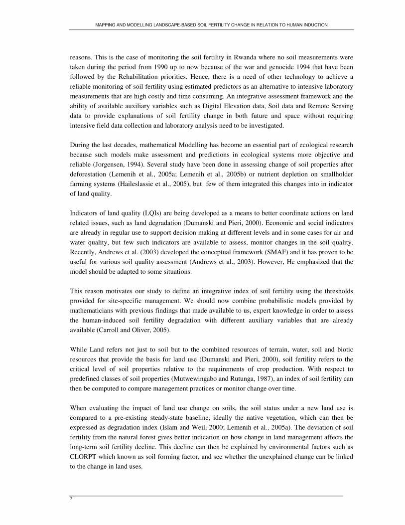
Changes in land use and land cover are central to the study of global environmental change. Among these changes is soil fertility degradation, which has become a major problem for agricultural management in Rwanda. Man as a soil-forming factor has been a difficult issue for pedology in general; explaining changes in soil fertility is but one example. The main agent causing change in processes controlling soil fertility is generally considered to be human activity. However, the nature and causes of soil fertility change in the complex lithology of Rwandan highlands is currently poorly known. In order to design and implement the national policy 2020 for conservation and restoration of soil fertility, policy makers need a clear and quantitative view of the spatio-temporal pattern of nutrient removal and redistribution, as well as the causes of decline. Existing detailed soil maps and lab analyses are more than 20 years old and poorly reflect the situation since the civil conflict of the 1990’s, which resulted in major land use changes. This study attempts a quantitative assessment of human-induced soil fertility change in the Gishwati watershed. To supplement the 1980’s soil map, a supplementary soil sampling, followed by lab analysis was carried out. Factor analysis was used to select most-significant fertility indicators (MSFI). These were used to develop a soil fertility index (SFI) and deterioration index (DI) which was interpolated over the study area for both dates. The soil fertility model was developed and validated using independent validation set. Kriging prediction was then applied to the data using auxiliary variables such soil mapping units and soil predictive components (SPC) generated from improved DEM and derived hydrological indices. The result of PCA showed that pH, OC, Al, P, K, Ca, and Mg are the most dynamic chemical properties in Rwanda (refer as MSFI), and those can be used to monitor the change in soil fertility over time. One-way ANOVA revealed that all MSFI are highly affected by LUCC with regards to soil type and topography. By computing the deviation of SFI from natural forest to other land uses, SFI captured the individual MSFI information, and revealed the change of soil fertility over 25 years. The soil fertility deterioration index (DI), which reflects the changes in soil fertility from natural forest conversion to different land uses with respect to soil type, revealed that soil quality in the study area has been significantly reduced in agricultural lands (-31%), pine plantations (-24%) and pasture land (-16%). However, DI showed that volcanic soils are slowly degraded compared acidic soils. With regular cultivation, Eutrandepts and Andaquepts lost only 7% over more than 11 years. Of the geostatistical analysis including SMUs and SPCs predictors, SFI was the best choice for representing spatial structure of soil fertility change in relation to LUCC. Prediction accuracy ranged from 91% to 93% in the entire Gishwati watershed. Therefore SFI maps differences enabled us to detect early degradation caused by different change in land uses done in different time which could not be easily seen using individual MSFI.
ii
Acknowledgements
I would like to express my sincere gratitude to the Government of Netherlands through the Netherlands Programme for the Institutional Strengthening of Post-secondary Education and Training Capacity (NPT) for granting me this opportunity to study for a Master of Science degree. I am grateful to my employer, the National University of Rwanda for providing me this opportunity to pursue higher studies. I want to express my gratefulness to my supervisors Dr D. Rossiter and Dr Ir C.A.J. M. de Bie for their excellent guidance. Without their direct assistance this thesis would not have been possible. Also, I would like to express my special thanks to Mr. Bart Krol for the encouragements throughout my study period and especially during the field work. His regular advisor made my studies successful. Thanks to Dr. M.J.C. Weir, Program Director of NRM for being our father throughout the studies. I would like to appreciate Ir. D. Ntawumenya, employer in the Ministry of Agriculture, for providing the soil and topographical data required for this study. I would like to extend my gratitude to Mr. J. Farifteh who always had time for me and had the advice ready. It was always a pleasure to discuss with him a draft of content of this thesis. I enjoyed the way he raised questions that always allowed me to dig more into the scientific content of my research. I would like to express my appreciation to ITC staff members, especially Dr. B.H.P. Maathuis for his fruitful advice. To Mr.G.Reinink, Mr. J.H.M.Hendrikse, Ir. W. Koolhoven, and Ir.V. Retsios for being helpful to me during the data analysis. I am also grateful to Rwanda Institute of Agriculture Research (ISAR), especially Mr. E. Gashabuka, researcher and head of ISAR-Gishwati station for providing logistic during field data collection. Thanks to Mr F. Mbarubukeye, technician at ISAR-Gishwati for enormous assistance in soil sample collection. My thanks extend to Mr. A. Ntawumenya and D. Shiragaga, technicians in PASI laboratory for their assistance during the laboratory analysis period. Their commitment and sacrifice of their time allowed me to complete this thesis on time. Thanks to fellow Rwandese students especially .P. Bizimana, F. Uwimana, V. Munyaburanga, C.M. Rulinda for our joint efforts that made Enschede a pleasant place to live during our studies at ITC. I would like to give special thanks to the NRM 2005 in particular S. Mungungu, R. Nyaribi, C. G. Mandara, Z. Newa, Matilda, A. Sedogo and Julie who provided their assistance in modules, and additionally, gave a pleasant touch to the difficult moments, making the situation bearable and enjoyable. This study would not have been possible without constant and valuable support from my family, particularly my lovely husband who day by day was behind my shoulders encouraging me and feeding my hopes to get successful results. Thanks to my son Jackson and my daughter Lillian, for their constant stimulation and for showing me the sense of our life. To my family members and friends who have been constantly interested in my progress with the studies. May God bless you all.

iii
Table of contents
1. Introduction ......................................................................................................................................1
1.1. Background .............................................................................................................................1 1.2. Research problem ...................................................................................................................2 1.3. Research objectives ................................................................................................................3 1.4. Research questions..................................................................................................................3 1.5. Hypotheses..............................................................................................................................3 1.6. Research approach ..................................................................................................................4
2. Concepts ...........................................................................................................................................6 2.1. Soil fertility degradation in relation to LUCC........................................................................6 2.2. Integrated approach for soil quality assesment and monitoring .............................................6 2.3. Prediction of soil fertility change using CLORPT model ......................................................8
3. Material and Methods ....................................................................................................................10 3.1. Gishwati study area in the context of Rwandan environment .............................................10
3.1.1. Climate, geology and geomorphology..............................................................................10 3.1.2. Soils and fertility ..............................................................................................................11 3.1.3. Historical land Use and Land cover change.....................................................................11
3.2. Research Methods.................................................................................................................13 3.2.1. Methodological flowchart ................................................................................................13 3.2.2. Spatial and temporal boundaries of the study ..................................................................14 3.2.3. Data types .........................................................................................................................14 3.2.4. Soil fertility change analysis ............................................................................................19 3.2.5. Soil fertility change interpretation....................................................................................20
4. Results ............................................................................................................................................25 4.1. Characterisation of soil fertility indicators and predictors ...................................................25
4.1.1. Land Use and Cover change (LUCC) over the 25 years and soil surveys .......................25 4.1.2. Variation of soils and soil samples locations ...................................................................27 4.1.3. Landscape complexity of Gishwati catchment area .........................................................27
4.2. Selection of the Minimum Soil Fertility Indicators .............................................................28 4.3. Change in soil fertility over 25 years....................................................................................30 4.4. Spatial variation of MSFI 2006 in relation to Ancillary Variables .....................................31
4.4.1. Variation of MSFI in relation to soil types ......................................................................32 4.4.2. Variation of MSFI in relation to Land Use change ..........................................................34 4.4.3. Variation of MSFI in relation to Landscape.....................................................................36
4.5. Relationships among soil fertility indicators ........................................................................38 4.6. Integration of Soil fertility indicators (MSFI) into index of soil quality (SFI) ....................38 4.7. Deterioration of soil fertility due to land use change ...........................................................40 4.8. Geostatistical analysis of soil fertility change ......................................................................41
4.8.1. Modelling the spatial structure of Soil fertility across Gishwati study area ....................41 4.8.2. Comparison of models in prediction of soil fertility ........................................................45 4.8.3. Models quality assessment ...............................................................................................46 4.8.4. Detection of the spatio-temporal soil fertility degradation ..............................................48

iv
5. Discussions.................................................................................................................................... 49 5.1. Determination of the Minimum Soil fertility Indicators (MSFI)......................................... 49 5.2. Trends of change in soil fertility indicators (MSFI) in relation to LUCC........................... 49 5.3. Performance of SFI model vs to MSFI models.................................................................... 50 5.4. Degradation of soil fertility in Gishwati highlands ............................................................. 51
6. Conclusions and recommendations ............................................................................................... 52 6.1. Conclusions.......................................................................................................................... 52 6.2. Recommendations................................................................................................................ 53
References ............................................................................................................................................. 54 Appendices ............................................................................................................................................ 58
v
List of figures
Figure 1-1: Conceptual diagram of soil fertility degradation (DI) in relation to land use system...........2 Figure 1-2: Decision tree for mapping and modelling soil fertility degradation using CLORPT approach ...................................................................................................................................................5 Figure 3-1: Map showing Gishwati study area before 1995 ..................................................................10 Figure 3-2: Methodological flowchart soil fertility change analysis and mapping. ..............................13 Figure 3-3: Soil series map of Gishwati study area ...............................................................................15 Figure 3-4: NDVI map of Gishwati study area using Aster, February 2005 .........................................17 Figure 3-5: Conceptual model of soil fertility index (SFI) development after Andrews et al. (Karlen et al., 2003).................................................................................................................................................21 Figure 4-1: Maps showing Land Covers of Gishwati in 1986 and 2006 ...............................................26 Figure 4-2: Change detection map showing the change in land cover over 25 years ............................26 Figure 4-3: Great group soils map of Gishwati study area and sample locations..................................27 Figure 4-4: Improved digital elevation map (DEM) of Gishwati catchment area .................................28 Figure 4-5: Boxplots of each soil fertility indicator by 25 years and the probability of significant difference using one-way ANOVA........................................................................................................31 Figure 4-6: Post plots of the minimum soil fertility indicators (MSFI) using 200 soil samples measured in the Gishwati study area......................................................................................................32 Figure 4-7: Boxplots showing MSFI variation in different type of soils ...............................................33 Figure 4-8: Box plots showing MSFI variation in different type of change in land use........................35 Figure 4-9: Soil fertility indicators for different landscape positions....................................................37 Figure 4-10: Contribution of original MSFI values in soil fertility index (SFI)....................................39 Figure 4-11: (a) variation of SFI in different soil types, (b) type of change in land use and (c) landscape positions ................................................................................................................................39 Figure 4-12: Deterioration index for different types of land use change...............................................40 Figure 4-13: (a) Post plot of SFI and (b) SFI histogram using 200 sample points of 2006 ...................41 Figure 4-14: Variogram models of indicators (MSFI) and resulted soil fertility model (SFI) ..............43 Figure 4-15: First four soil predictive components from terrain parameters.........................................44 Figure 4-16: Gaussian model of SFI residuals .......................................................................................45 Figure 4-17: Gaussian model of SFI residuals after stratifying SPCs by SMUs ...................................45 Figure 4-18: Predicted soil fertility map (a) by OK, (b) by RK using SPCs , and (c) by RK using SMUs as strata of SPCs..........................................................................................................................46 Figure 4-19: Comparison of models performance at interpolation set (a: OK, b: RK with SPCs, and c: RK with SPCs stratified by SMUs)........................................................................................................47 Figure 4-20: Comparison of model performance at validation set (a: OK, b: RK with SPC, and c: RK with SMUs) ............................................................................................................................................47 Figure 4-21: Predicted error map (a) by OK, (b) by RK using SPC, (c) by RK using SMUs as strata of SPCs .......................................................................................................................................................48 Figure 4-22: Soil fertility index (SFI) maps for both years (1981 and 2006) and soil fertility deterioration (DI) map resulted on differences ......................................................................................48
vi
List of tables
Table 3-1: Unit conversion coefficients and mean exoatmospheric irradiance of ASTER bands........ 17 Table 3-2: Data type and key variables considered for soil fertility change analysis........................... 18 Table 4-1: Great group soils of Gishwati and series that are represented............................................. 27 Table 4-2: Statistics’ values of terrain parameters included in soil-landscape modeling..................... 28 Table 4-3: Matrix of nonparametric correlations of 14 soil fertility indicators (SFI) in the topsoil from Rwanda (Spearman correlation: r). ....................................................................................................... 29 Table 4-4: Loadings of the first four components (PC) from PCA of 16 SFIs in topsoil of Rwanda... 30 Table 4-5: Multiple comparison of MSFI means by soil type and separations using Duncan test ....... 34 Table 4-6: Multiple comparison of MSFI means by type of change in land use and separations using Duncan test ............................................................................................................................................ 36 Table 4-7: Multiple comparison of MSFI means by landscape and separations using Duncan test..... 37 Table 4-8: Spearman correlations among MSFI using 200 soil observations points............................ 38 Table 4-9: Multiple comparisons of SFI Means by soil type, land use change and landscape............. 40 Table 4-10: Mean separation of DI by Duncan test .............................................................................. 40 Table 4-11: Factor analysis matrix of landscape predictors.................................................................. 43
vii
List of appendices
Appendix 1: Field-Data Collection Form for Soil Fertility Mapping and Modelling ...........................58 Appendix 2: Soil series of Gishwati ......................................................................................................59 Appendix 3: Descriptive Statistics of 15 soil properties of topsoil of Rwanda.....................................60 Appendix 4: Summary statistics of revisited soil profiles of CPR 1981 (MSFI 1981, N=17) ..............60 Appendix 5: Summary statistics of MSFI 2006 on the revisited MSFI 1981 (N=17) ...........................60 Appendix 6: Summary Statistics of MSFI 2006 ....................................................................................61 Appendix 7: One-way ANOVA showing the significant change of MSFIs over 25 years....................61 Appendix 8: One-way ANOVA of MSFI by Soil types.........................................................................61 Appendix 9: One-way ANOVA of MSFI by type of change in land use...............................................61 Appendix 10: One-way ANOVA of MSFIs by Landscape position......................................................61 Appendix 11: Thresholds for interpretation of the pH results (after Mutwewingabo et al., 1987) .......62 Appendix 12: Thresholds for interpretation of Soil nutrients availability (P, K, Ca, and Mg) .............62 Appendix 13: Thresholds for interpretation of the results of org. carbon and Aluminum acidity ........62 Appendix 14: Spatial correlation of SFI observation points..................................................................63 Appendix 15: Linear relationship between soil types and soil fertility index (SFI) (R2=0.15) .............63

viii
List of abbreviations
ANOVA Analysis of variance ASTER Advanced Space-borne Thermal Emission and Reflection Radiometer BADC Belgium Administration for Development Cooperation CPR Carte Pedologique du Rwanda DBF Database file DI Deterioration Index DEM Digital elevation map DN Digital Number DTM Digital Terrain Model FA Factor Analysis ILWIS Integrated Land and Water Information System software GLASOD Global Assessment Degradation GLM Generalised Linear Model KED Kriging with External Drift LP Landscape position LUCC Land Use and Land Cover Change MDS Minimum Data Set MPE Mean Prediction Error MSFI Minimum Soil Fertility Indicators MLC Maximum Likelihood Classifier MINITERRE Ministere of Land, Environment, Forestry, Water and Mines NUR National University of Rwanda NDVI Normalized Difference Vegetation Index NMSE Normalized Mean Square Error OK Ordinary Kriging PCA Principal Component Analysis PCFN Nyungwe Forest Conservation Project RK Regression Kriging RMSPE Root Mean Square Prediction Error SCM Spearman Correlation Matrix SFI Soil Fertility Index SFID Soil Fertility Index Development SHP Shape file SMU Soil Mapping Unit SPC Soil Predictive Component SPI Stream Power Index STI Sediment Transport Index TM Thematic Mapper TWI Topographic Wetness Index WCS Wildlife Conservation Society WLS Weighted Least Square
MAPPING AND MODELLING LANDSCAPE-BASED SOIL FERTILITY CHANGE IN RELATION TO HUMAN INDUCTION
1
1. Introduction
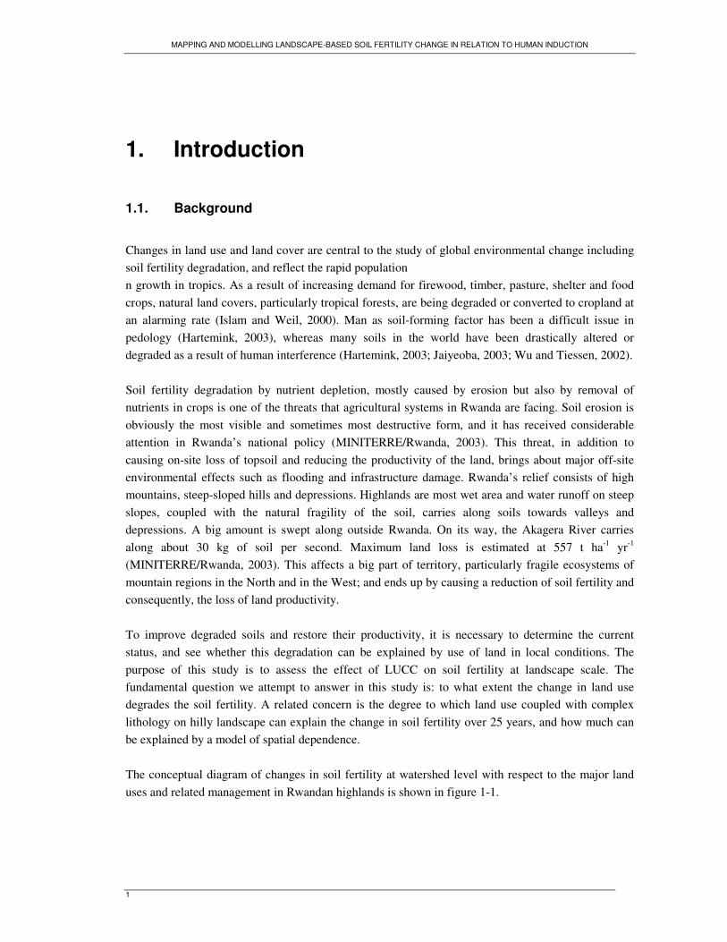
1.1. Background
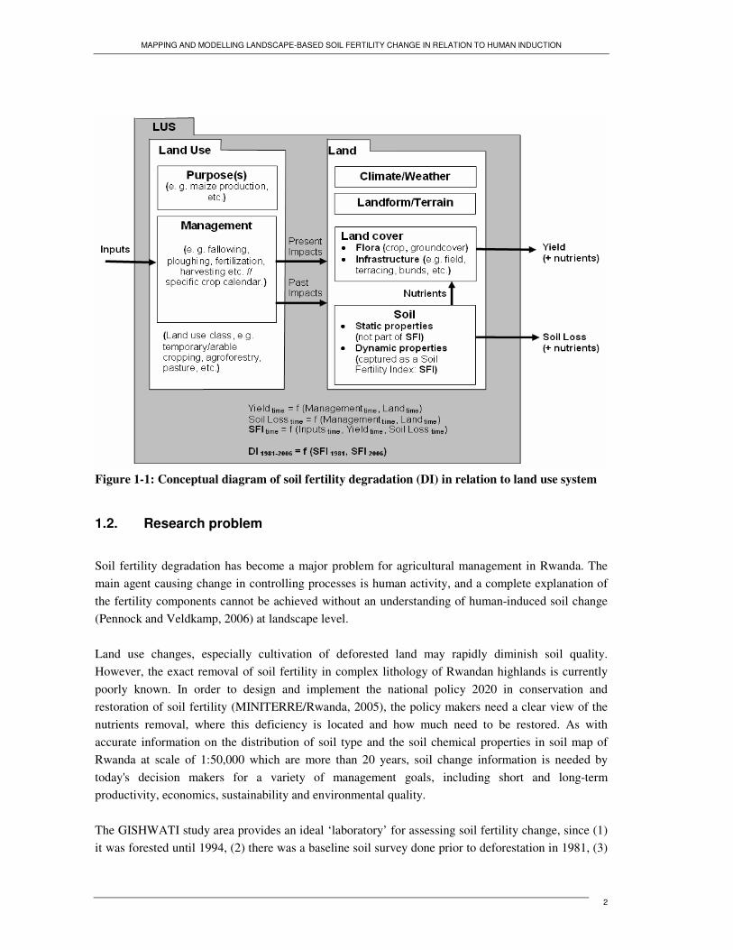
Changes in land use and land cover are central to the study of global environmental change including soil fertility degradation, and reflect the rapid population n growth in tropics. As a result of increasing demand for firewood, timber, pasture, shelter and food crops, natural land covers, particularly tropical forests, are being degraded or converted to cropland at an alarming rate (Islam and Weil, 2000). Man as soil-forming factor has been a difficult issue in pedology (Hartemink, 2003), whereas many soils in the world have been drastically altered or degraded as a result of human interference (Hartemink, 2003; Jaiyeoba, 2003; Wu and Tiessen, 2002). Soil fertility degradation by nutrient depletion, mostly caused by erosion but also by removal of nutrients in crops is one of the threats that agricultural systems in Rwanda are facing. Soil erosion is obviously the most visible and sometimes most destructive form, and it has received considerable attention in Rwanda’s national policy (MINITERRE/Rwanda, 2003). This threat, in addition to causing on-site loss of topsoil and reducing the productivity of the land, brings about major off-site environmental effects such as flooding and infrastructure damage. Rwanda’s relief consists of high mountains, steep-sloped hills and depressions. Highlands are most wet area and water runoff on steep slopes, coupled with the natural fragility of the soil, carries along soils towards valleys and depressions. A big amount is swept along outside Rwanda. On its way, the Akagera River carries along about 30 kg of soil per second. Maximum land loss is estimated at 557 t ha-1 yr-1 (MINITERRE/Rwanda, 2003). This affects a big part of territory, particularly fragile ecosystems of mountain regions in the North and in the West; and ends up by causing a reduction of soil fertility and consequently, the loss of land productivity. To improve degraded soils and restore their productivity, it is necessary to determine the current status, and see whether this degradation can be explained by use of land in local conditions. The purpose of this study is to assess the effect of LUCC on soil fertility at landscape scale. The fundamental question we attempt to answer in this study is: to what extent the change in land use degrades the soil fertility. A related concern is the degree to which land use coupled with complex lithology on hilly landscape can explain the change in soil fertility over 25 years, and how much can be explained by a model of spatial dependence. The conceptual diagram of changes in soil fertility at watershed level with respect to the major land uses and related management in Rwandan highlands is shown in figure 1-1.
MAPPING AND MODELLING LANDSCAPE-BASED SOIL FERTILITY CHANGE IN RELATION TO HUMAN INDUCTION
2
Figure 1-1: Conceptual diagram of soil fertility degradation (DI) in relation to land use system
1.2. Research problem
Soil fertility degradation has become a major problem for agricultural management in Rwanda. The main agent causing change in controlling processes is human activity, and a complete explanation of the fertility components cannot be achieved without an understanding of human-induced soil change (Pennock and Veldkamp, 2006) at landscape level. Land use changes, especially cultivation of deforested land may rapidly diminish soil quality. However, the exact removal of soil fertility in complex lithology of Rwandan highlands is currently poorly known. In order to design and implement the national policy 2020 in conservation and restoration of soil fertility (MINITERRE/Rwanda, 2005), the policy makers need a clear view of the nutrients removal, where this deficiency is located and how much need to be restored. As with accurate information on the distribution of soil type and the soil chemical properties in soil map of Rwanda at scale of 1:50,000 which are more than 20 years, soil change information is needed by today's decision makers for a variety of management goals, including short and long-term productivity, economics, sustainability and environmental quality. The GISHWATI study area provides an ideal ‘laboratory’ for assessing soil fertility change, since (1) it was forested until 1994, (2) there was a baseline soil survey done prior to deforestation in 1981, (3)

MAPPING AND MODELLING LANDSCAPE-BASED SOIL FERTILITY CHANGE IN RELATION TO HUMAN INDUCTION
3
the area has been deforested since 1995, and due to Agricultural and Settlement activities, it has faced dramatic erosion and changes in soil management, in particular intensive cropping.
1.3. Research objectives
The present study aimed to investigate and map the evolution of soil fertility in Rwandan highland as a result of land use change and related management. The main objective of this research was to quantify the response of soil fertility to human activity in Rwandan highlands at watershed level. The related concerns were to map the spatial distribution of soil fertility using auxiliary variables that were available and to model the temporal evolution of soil fertility within a watershed. To accomplish this, a minimum data set (MDS) for soil fertility changes were developed; and used to determine soil fertility index (SFI) that were used to predict the spatial distribution of changes across different soil types and present land uses of entire Gishwati catchment area.
1.4. Research questions
1) What is the Minimum Data Set (MDS) of soil chemical attributes that can be used to assess
the landscape-based soil fertility change? 2) Is there a significant change in soil fertility over the last 25 years? If so, what is it, and where
are the changes most pronounced? 3) How can the individual indicators of soil fertility be modeled into and integrative measure of
soil fertility and fertility degradation? 4) To what extent land use change contributes to soil fertility change at watershed level? 5) How successfully can the spatial pattern of soil fertility be predicted in complex lithology of
Rwandan highlands?
1.5. Hypotheses
1) Soil Nutrients are the most dynamic soil fertility indicators. Those can be used for soil
fertility change mapping and modelling. 2) The soil fertility indicators have changed significantly over the last 25 years, especially in
areas invaded since 1980. 3) Soil fertility indicators are modeled into Soil Fertility Index (SFI) and Fertility Deterioration
Index (DI) using thresholds values of soil properties classes of Rwanda. 4) There is significant difference in soil fertility within the same soil forming environment.
These differences are highly explained by the type of change in land use. 5) The spatial change in soil fertility is fairly mapped using Kriging methods that include soil
forming factors in the model of spatial dependence than using only the target variable.
MAPPING AND MODELLING LANDSCAPE-BASED SOIL FERTILITY CHANGE IN RELATION TO HUMAN INDUCTION
4
1.6. Research approach
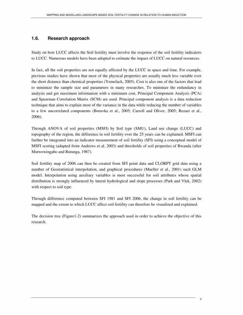
Study on how LUCC affects the Soil fertility must involve the response of the soil fertility indicators to LUCC. Numerous models have been adopted to estimate the impact of LUCC on natural resources. In fact, all the soil properties are not equally affected by the LUCC in space and time. For example, previous studies have shown that most of the physical properties are usually much less variable over the short distance than chemical properties (Yemefack, 2005). Cost is also one of the factors that lead to minimize the sample size and parameters in many researches. To minimize the redundancy in analysis and get maximum information with a minimum cost, Principal Component Analysis (PCA) and Spearman Correlation Matrix (SCM) are used. Principal component analysis is a data reduction technique that aims to explain most of the variance in the data while reducing the number of variables to a few uncorrelated components (Boruvka et al., 2005; Carroll and Oliver, 2005; Rezaei et al., 2006). Through ANOVA of soil properties (MSFI) by Soil type (SMU), Land use change (LUCC) and topography of the region, the difference in soil fertility over the 25 years can be explained. MSFI can further be integrated into an indicator measurement of soil fertility (SFI) using a conceptual model of MSFI scoring (adapted from Andrews et al. 2003) and thresholds of soil properties of Rwanda (after Mutwewingabo and Rutunga, 1987). Soil fertility map of 2006 can then be created from SFI point data and CLORPT grid data using a number of Geostatistical interpolation, and graphical procedures (Mueller et al., 2001) such GLM model. Interpolation using auxiliary variables is most successful for soil attributes whose spatial distribution is strongly influenced by lateral hydrological and slope processes (Park and Vlek, 2002) with respect to soil type. Through difference computed between SFI 1981 and SFI 2006, the change in soil fertility can be mapped and the extent to which LUCC affect soil fertility can therefore be visualized and explained. The decision tree (Figure1-2) summarizes the approach used in order to achieve the objective of this research.
MAPPING AND MODELLING LANDSCAPE-BASED SOIL FERTILITY CHANGE IN RELATION TO HUMAN INDUCTION
5
Figure 1-2: Decision tree for mapping and modelling soil fertility degradation using CLORPT approach
Soil properties of the topsoil of Rwanda in 1981
1. What are the most dynamic?
Dynamic properties MSFI
Static properties
MSFI 2006
2a. Is there a significant difference?
SFI 2006 (Point map)
3. How can MSFI be integrated into an index of soil fertility?
MSFI 1981
If yes
SFI 1981 (Polygon map)
4. To what extent LUCC contribute to SFI change (DI)?
5a. Do CLORPT factors explain SFI variation?
If yes
5b. How successful is to map SFI 2006 using available CLORPT
Predicted SFI map & Error of prediction
2b. How much and where the changes are most pronounced?
DI map
PCA & SCM
One-way ANOVA
GLM
RK
One-way ANOVA
SFID model
MAPPING AND MODELLING LANDSCAPE-BASED SOIL FERTILITY CHANGE IN RELATION TO HUMAN INDUCTION
6
2. Concepts
2.1. Soil fertility degradation in relation to LUCC
Land use and land cover change (LUCC) plays an important role in soil fertility dynamics when compared with natural factors, and can have impact upon soil quality especially under tropical climate conditions. Soil fertility defined as ‘the quality of a soil that enables it to provide nutrients in adequate amounts and proper balance for the specified plants or crops’ has been the cause for much debate and the high fertility theory of tropical soils was dispelled when the forest was cut, crops planted and it was discovered that yield levels were disappointingly low or rapidly declining (Hartemink, 2003). But, this effect of LUCC focuses on short term changes such as deforestation. Other less dramatic decadal scale land use changes turn out to have less effect on soil properties, especially when the results are corrected for landscape variability (Breuer et al., 2006). An assessment of soil properties upon conversion of natural forests for different purposes is of utmost importance to detect early changes in soil quality. This has been basically proved significant in a tropical forest ecosystem of Bangladesh (Islam and Weil, 2000). Yet, Global change research has stimulated research on the fate of soil organic carbon in relation to soil management and land use change (Pennock and Veldkamp, 2006). However, previous studies have generally not considered landscape relations. These changes might behave differently with regard to lithology variability within the same landscape. Three different data types are used to assess soil changes caused by agriculture production systems: expert Knowledge, nutrient balances and monitoring of soil chemical properties over time (Type I) or at different sites (Type II). Changes can be assessed by measuring and comparing present values against values at the commencement of the monitoring period (Arshad and Martin, 2002), with historical data when available, with soil attributes under reference ecosystems (Wang and Gong, 1998), or using values measured at different time intervals. This is so called chronosequential sampling or Type (I) data. Type I data show changes in soil chemical property under a particular type of land use change over time whereas with type II data, soil under adjacent different land use systems are sampled at the same time and compared (Hartemink, 2003). Therefore, in this study we focus on both types due to the lower number of type I samples. Moreover, Type II data allows spatial and temporal change while Type I data allows only temporal change analysis.
2.2. Integrated approach for soil quality assesment and monitoring
Identification of soil nutrient deficiencies is usually carried out through the analysis of the soil. Nonetheless, this process can be expensive and time consuming, depending on the extent of the area to be evaluated. In other hand, the time series measurements are not always available due to different
MAPPING AND MODELLING LANDSCAPE-BASED SOIL FERTILITY CHANGE IN RELATION TO HUMAN INDUCTION
7
reasons. This is the case of monitoring the soil fertility in Rwanda where no soil measurements were taken during the period from 1990 up to now because of the war and genocide 1994 that have been followed by the Rehabilitation priorities. Hence, there is a need of other technology to achieve a reliable monitoring of soil fertility using estimated predictors as an alternative to intensive laboratory measurements that are high costly and time consuming. An integrative assessment framework and the ability of available auxiliary variables such as Digital Elevation data, Soil data and Remote Sensing data to provide explanations of soil fertility change in both future and space without requiring intensive field data collection and laboratory analysis need to be investigated. During the last decades, mathematical Modelling has become an essential part of ecological research because such models make assessment and predictions in ecological systems more objective and reliable (Jorgensen, 1994). Several study have been done in assessing change of soil properties after deforestation (Lemenih et al., 2005a; Lemenih et al., 2005b) or nutrient depletion on smallholder farming systems (Haileslassie et al., 2005), but few of them integrated this changes into in indicator of land quality. Indicators of land quality (LQIs) are being developed as a means to better coordinate actions on land related issues, such as land degradation (Dumanski and Pieri, 2000). Economic and social indicators are already in regular use to support decision making at different levels and in some cases for air and water quality, but few such indicators are available to assess, monitor changes in the soil quality. Recently, Andrews et al. (2003) developed the conceptual framework (SMAF) and it has proven to be useful for various soil quality assessment (Andrews et al., 2003). However, He emphasized that the model should be adapted to some situations. This reason motivates our study to define an integrative index of soil fertility using the thresholds provided for site-specific management. We should now combine probabilistic models provided by mathematicians with previous findings that made available to us, expert knowledge in order to assess the human-induced soil fertility degradation with different auxiliary variables that are already available (Carroll and Oliver, 2005). While Land refers not just to soil but to the combined resources of terrain, water, soil and biotic resources that provide the basis for land use (Dumanski and Pieri, 2000), soil fertility refers to the critical level of soil properties relative to the requirements of crop production. With respect to predefined classes of soil properties (Mutwewingabo and Rutunga, 1987), an index of soil fertility can then be computed to compare management practices or monitor change over time. When evaluating the impact of land use change on soils, the soil status under a new land use is compared to a pre-existing steady-state baseline, ideally the native vegetation, which can then be expressed as degradation index (Islam and Weil, 2000; Lemenih et al., 2005a). The deviation of soil fertility from the natural forest gives better indication on how change in land management affects the long-term soil fertility decline. This decline can then be explained by environmental factors such as CLORPT which known as soil forming factor, and see whether the unexplained change can be linked to the change in land uses.
MAPPING AND MODELLING LANDSCAPE-BASED SOIL FERTILITY CHANGE IN RELATION TO HUMAN INDUCTION
8
2.3. Prediction of soil fertility change using CLORPT model
Global Assessment of Soil Degradation (GLASOD, 1990) has shown that the soil chemical degradation is believed to be important in many parts of the tropics. The loss of nutrient (i.e. soil fertility decline) is severe in Africa (Hartemink, 2003) including a large part of Rwanda. The method of Geographic information System (GIS) for soil nutrients mapping using different types of interpolation is well proposed and is being used in soil science (Amini et al., 2005; Bishop and McBratney, 2001; Iqbal et al., 2005; Lark and Ferguson, 2004; Li et al., 2004; Liu et al., 2006; McBratney et al., 2003; Mueller and Pierce, 2003; Mueller et al., 2004a; Mueller et al., 2004b; Srivastava and Saxena, 2004). In this chapter, we discuss the various methods that have been used to map the soil properties which are used to monitor the soil fertility change. We also review the soil-environment relationship that has been widely used in soil mapping and modelling. Jenny's equation (1941) is known as the first model of soil development,
),,,,( tprocfS = , (1)
Where S represents a soil attribute (e.g. fertility) or soil class, c (sometimes cl) climate, o organisms including human activity, r relief, p parent material and t time. Most of the soil models are built based on this famous equation. Numerous researchers have taken the quantitative path and have tried to formalize this equation largely through studies of cases where one factor varies and the rest are held constant. Since the 1960s, there has been an emphasis on what might be called geographic or purely spatial approaches in soil mapping. Soil attribute can be predicted from spatial position largely by interpolating between soil observation locations where soil is considered at some location (x,y) to depend on the geographic coordinates x,y and on the soil at neighbouring locations (x + u, y + v), i.e.,
),(),,((),( vyuxsyxfyxS ++= . (2) These purely spatial approaches are almost entirely based on Geostatistics and its precursor trend-surface analysis. Geostatistics provides descriptive tools such as semi-variogram to characterize the spatial pattern of continuous and categorical soil attributes (Amini et al., 2005; Lark and Ferguson, 2004). This technique has been widely applied by soil scientists particularly, various forms of kriging. However, it was recognised early in the development of soil Geostatistics that soil could be better predicted if denser sets of secondary variables correlated with the primary variable were available (McBratney et al., 2003). This technique is called co-kriging, regression kriging, or kriging with external drift:
),)(,,,,{),,((),( yxtproclvyuxsfyxS ++= . (3)
In the early co-kriging studies (e.g. in 1983), these secondary variables were other soil variables, indicating that other soil variables are themselves useful predictors of soil. Later in 1994, with the advent of GIS and improved technology, Odeh et al.(1994) found that co-kriging can be performed with detailed auxiliary data sets of environmental variables derived from digital elevation models and
MAPPING AND MODELLING LANDSCAPE-BASED SOIL FERTILITY CHANGE IN RELATION TO HUMAN INDUCTION
9
satellite images (McBratney et al., 2003). In the middle of the 1990s some researchers recognized the similarities between co-Kriging and regression Kriging. In the last approach ‘CLORPT’ is used to predict the soil property of interest from environmental variables and kriging is used on the residuals. In many cases, kriging combined with regression has proven to be superior to the plain Geostatistical techniques yielding more detailed results and higher accuracy of prediction (Hengl et al., 2004b). Moreover, in several other studies (Bishop and McBratney, 2001; Simbahan et al., 2006), combination of kriging and correlation with auxiliary data outperformed ordinary kriging, co-kriging and plain regression. Kriging with external drift (KED) is an example of Kriging combined with regression which only allows a linear relationship between the variable of interest and the environmental variables (the external drifts). Although, quantitative relationships have generally been most easily found between soil and topography but the results of many studies illustrate that this empirical relationships between soil properties and terrain attributes are somewhat unique to each soil property and each soil-forming environment. Especially over large areas, predictive capabilities are limited because the relationships between soil properties and landscape attributes are nonlinear or unknown (Lagacherie and Voltz, 2000). In this view, the drift and residuals can also be fitted separately and then summed afterwards (Hengl et al., 2004b). This technique was originally suggested by Odeh et al. (1994, 1995), who named it ‘‘Regression Kriging’’ (RK), whereas Goovaerts uses the term ‘‘Kriging after detrending’’(Goovaerts, 1999). RK can be more easily combined with stratification, General Additive Modelling (GAM) and regression trees (McBratney et al., 2000). Recently, Multivariate RK with elevation, apparent EC, reflectance, and soil series performed best in terms of increasing map accuracy. For example, in multivariate RK methods relative improvements in map accuracy over OK ranged from 19% to 38% at the three sites in Nebraska and there was little loss of accuracy when sampling intensity was reduced by half (Simbahan et al., 2006). Therefore, in this study, we focuses on regression kriging (RK) instead of kriging with external drift (KED), not because, RK implies the regression combined with kriging, but it as well allows the nonlinear relationship between the target variable and continuous and categorical predictor. Numerous ancillary variables with potential for soil fertility mapping are available, particularly at landscape scale. Examples include digitized soil surveys (soil mapping units), digital elevation model (DEM) and derived terrain indices. DEM is useful to derive Slope gradient and aspect, the specific Catchment, and the hydrological terrain parameters that are used in Soil loss (Shrestha et al., 2004) as well as soil attributes prediction for a relatively large area (Ziadat, 2005). A methodological approach is also developed (Hengl et al., 2004b). The challenge is to apply them to the local environment, and produce an explicit soil fertility map with regard to covering the variation in primary and secondary variables in feature and geographical space in situation where the sampling intensity is limited.
MAPPING AND MODELLING LANDSCAPE-BASED SOIL FERTILITY CHANGE IN RELATION TO HUMAN INDUCTION
10
3. Material and Methods
3.1. Gishwati study area in the context of Rwandan environment
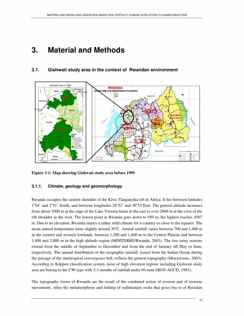
Figure 3-1: Map showing Gishwati study area before 1995
3.1.1. Climate, geology and geomorphology
Rwanda occupies the eastern shoulder of the Kivu–Tanganyika rift in Africa. It lies between latitudes 1o04’ and 2o51’ South, and between longitudes 28o53’ and 30o53’East. The general altitude increases from about 1000 m at the edge of the Lake Victoria basin in the east to over 2600 m at the crest of the rift shoulder in the west. The lowest point in Rwanda goes down to 950 m, the highest reaches 4507 m. Due to its elevation, Rwanda enjoys a rather mild climate for a country so close to the equator. The mean annual temperature turns slightly around 20oC. Annual rainfall varies between 700 and 1,400 m in the eastern and western lowlands, between 1,200 and 1,400 m in the Central Plateau and between 1,400 and 2,000 m in the high altitude region (MINITERRE/Rwanda, 2003). The two rainy seasons extend from the middle of September to December and from the end of January till May or June, respectively. The annual distribution of the orographic rainfall, issued from the Indian Ocean during the passage of the intertropical convergence belt, reflects the general topography (Moeyersons, 2003). According to Köppen classification system, most of high elevation regions including Gishwati study area are belong to the CW-type with 2-3 months of rainfall under 60 mm(ABOS-AGCD, 1983). The topography forms of Rwanda are the result of the combined action of erosion and of tectonic movements. After the metamorphosis and folding of sedimentary rocks that gives rise to of Rusizian
Kanama
Gasiza
Gaseke
Mutura
KayoveRutsiro
Cyanzarwe
Buhoma
Nyagisagara
Gishwati Natural Reserve
MilitaryDomain
Gishwati Area in 1988
1 0 1 2 Kilometers
Study zone boundaryNatural reserveThe plantationPasture landWoodlandDistrict BoudarySecondary roadRoad unpavedRoad paved
N
To Gisenyi
To Ruhengeri
To Kibuye
MAPPING AND MODELLING LANDSCAPE-BASED SOIL FERTILITY CHANGE IN RELATION TO HUMAN INDUCTION
11
and Burundian, the northern part of the country, including the Gishwati study area is underlain by Precambrian rusizian rocks composed of a wide range of shales locally pierced by granitic batholiths. These granites give way to more rounded hills and valleys than the shales and result a “landscape of thousand hills” with steep slope that characterized the “Congo-Nile watershed divide” in West (Moeyersons, 2003). The investigated area is within the Congo-Nile watershed divide in Western province of Rwanda (Figure 3). This area was chosen because of its representative of complex lithology and landscape diversity due to elevation differences from valley floor to mountain summits, and related land use changes having influence on soil erosion which is considered typical for the highland of Rwanda. It extends from easting of 29o21’40” to 29o28’50” longitude and southing of 1o36’52” to 1o52’17” latitude.
3.1.2. Soils and fertility
Soils of Rwanda present a high variability in physical and chemical properties. As reported by different researchers, most soils are fine textured, but the soil depth is strongly variable as well as weathering intensity and chemical soil fertility (Mukashema, 2003; Mutwewingabo, 1984; Neel et al., 1976; Ntaneza, 1988; Zaag, 1981; Zaag et al., 1982). Consequently, most of the Soil Taxonomy (Soil Survey Staff, 1983) orders are found in Rwanda (Verdoodt and Van Ranst, 2006), except Spodosols (ABOS-AGCD, 1983). In high elevation region where Gishwati watershed is located, Entisols occupy the river valleys; these are mostly Aquents. Histosols are very common in the poorly drained swamps. They are not typical for Gishwati but they occur elsewhere in Rwanda where the drainage is low. In the zones covered by volcanic material and, elsewhere on steep slopes, the Inceptisols are an extensive soil unit. Many soils developed in the colluviums accumulated at the foot of the hill slopes belong to this order too. Most well-drained soils of this region are belonging to Ultisols. In spite of the steep slopes, soils are generally deep and rich in organic matter. Some of the soils show a structure which could make them considered as Oxisols but generally their exchange capacity exceeds the value which is necessary for Oxisols (ABOS-AGCD, 1983). Speaking about soil fertility, we must stress that besides the classic pedogenetic factors, human activity did largely influence to the soil fertility status. This human influence, together with relief, explain why there is a wide range in crop yields over small distance, even in soils developed in the same parent material.
3.1.3. Historical land Use and Land cover change
The change in land use in Rwanda especially in Gishwati study area is result of the changes in population, which doubled nationally between 1978 and 2002. Over 90 percent of the population relies on subsistence agriculture to meet its needs, with a concomitant need for land, which puts great pressure on the country’s remaining natural ecosystems, whether forested, savannas, or wetland (Plumptre et al., 2001).

MAPPING AND MODELLING LANDSCAPE-BASED SOIL FERTILITY CHANGE IN RELATION TO HUMAN INDUCTION
12
Since 1980s, Gishwati forest reserve had been heavily affected by human activities prior to the Rwandan civil war. It constituted approximately 280 square kilometres in the mid-1970s and contained populations of chimpanzees (Pan Troglodytes) and golden monkeys (Cercopithecus mitis kandti), although the forest was fairly degraded by many years of cattle herding within the forest. The World Bank supported an integrated forestry and livestock project that converted 100 square kilometres to pasture and another 100 square kilometres to pine plantations in the early 1980s. A 30 square kilometres area was designated as a military zone in the north of the forest, leaving only 50 square kilometres of natural forest. During and following the war in 1994, the northern part of Gishwati was used for camps of displaced persons, which grew rapidly. People settled and farmed within the reserve, thus creating further pressures on land and deforestation. In early 2000, the Nyungwe forest conservation project (PCFN), supported by the Wildlife Conservation Society (WCS), organized a survey of Gishwati natural forest to assess the current status and to determine whether it would be useful to encourage conservation efforts. There was little of the original forest remaining in Gishwati. Only a few stands of trees of less than one hectare in size within cropland were observed (Plumptre et al., 2001).
MAPPING AND MODELLING LANDSCAPE-BASED SOIL FERTILITY CHANGE IN RELATION TO HUMAN INDUCTION
13
3.2. Research Methods
3.2.1. Methodological flowchart
����
�������
� ���
�� ��������
����������
� ���������������
� �� ��������
�� ���������
�� �������! �"
�����
�� #����
$ �%��&����
�����
���&�'&��
$ ����&�� �
�&$� ��&�&�(����
����
� ����&'����
$ ���$�� �
��&)�&�&�(���
��&��&��&�&�(�����*�
�'�� �'����
&�%�&�&(���
+,���
+��
�����-../
���%&�&
+&�%�&�0/�*1����2
����-../1�-..2�
�� '����$�&�%��&%� '����$�
$&��)�&�� �
3�45�$&�$��&�� �
*��5�
����
*��5�
-..2
�3�4� #�*��5�
)(��'�
�����#�$&���
%�##����$�
�*,� ��*�1��+���1�
��51��51�65
�&$� ��&�&�(���
3�4� #�*��5�)(��*,�1�
+,���&�%�+�
&�%�� ���� $�����
�����#�$&���
%�##����$��
� ������%�$�� ��
$ '� ������
������
5�����&�� �� #�
*��5����� ���5
*��5�
����
�����
��5�����
�����
��5�-..2
�����
�5��&�&�(���
��5�-..2�
5����� �&�� �����
�� ����'&��
��5�-..2
&��%&�� �����
�� ����'&��
�5���5�������
�����&�%��*,�
��+*�
��&��&��
&�� $ ����&�� ��
&�&�(���
���%��
����'&���
��&��&��
&�� $ ����&�� �� #�
�������� ��
����%�&��
5����� �&
������%�
&�����7�
���&�����%�$�� ��'&��� &��&���
&$$��&$(� #����%�$�� �
���%�$��%���5
,������7
��&���#��%��
*0/�
���2
����� ���%�
��&���#�$&�� ���*+��
� &��&�������$�&���������5
� ���#�������(�%���&%&�� ��'&�
��5�
3�45�'&��
��/.1...�
��&���#��%�
����
-..2
+&�%�����
$�&�����+,����
'&�
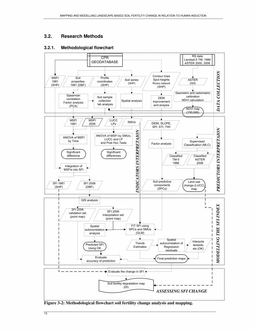
Figure 3-2: Methodological flowchart soil fertility change analysis and mapping.
DA
TA C
OLL
EC
TIO
N
IND
ICA
TOR
S IN
TER
PRE
TAIO
N
PR
ED
ICTO
RS
INTE
RPR
ETA
ION
MO
DE
LLIN
G T
HE
SF
I IN
DE
X
ASSESSING SFI CHANGE
MAPPING AND MODELLING LANDSCAPE-BASED SOIL FERTILITY CHANGE IN RELATION TO HUMAN INDUCTION
14
3.2.2. Spatial and temporal boundaries of the study
To assess soil fertility decline, it is necessary to define the spatial and temporal boundaries of the system under study. The loss of fertility by erosion at catchment scale is measured spatially using the black box approach. This approach considers the depth, the width and length as important boundaries of the box. The same approach is used to explain the transfer of nutrients from one area or spatial scale to another by subsurface flow (Hartemink, 2003). This approach was applied to this study. Gishwati catchment represents a catena of about 280 km2 with flows of nutrients from upper slope to valley by erosion or subsurface flow process. The depth of the box was about 30 cm as the most vulnerable layer to erosion and most important for crop growth. The study focused firstly on different land uses for the entire area and for the temporal study, the profiles of 1981 project were also revisited.
3.2.3. Data types
3.2.3.1. Soil fertility indicators
To assess the change in soil fertility at a given site, Type I data were used. This method is also called chronosequential sampling or Type (I) data. Type I data show changes in soil chemical property under a particular type of land use change over time. Usually the original level is taken as the reference level to investigate the trend in such changes. Example, Type I data have been used for quantifying soil contamination by comparing soil samples collected before the intensive industrialization period with recent samples taken from the same location (Hartemink, 2003). The same approach was used to quantify the change in soil fertility of the study area. We used the chemical properties already measured from 1981 through the semi-detailed soil survey done during the project named “Carte pedologique du Rwanda” (CPR), and compared to newly collected and analysed soil samples of 2006. Because there were only 17 points of Type I which was not even distributed in different land uses, the land use change effect on soil fertility was assessed using Type II data. In this approach, soil fertility status under adjacent different land use systems were sampled and compared. This is so called biosequential sampling (Hartemink, 2003) or synchronic sampling (Yemefack, 2005). The main underlying assumption is that the soils on the cultivated land, pasture, planted forest and reference land use (in this case natural forest) are the same soil type (refer to great group units), but that the differences in soil fertility can be attributed to the difference to the differences in land use. Revisiting the site is the key for Type I data, while knowing the historical land use is much more important for Type II. Both types were involved in assessing the spatio-temporal change of soil fertility across Gishwati catchment area. Type II was useful for spatial distribution of the change whereas Type I was important for temporal change analysis.
MAPPING AND MODELLING LANDSCAPE-BASED SOIL FERTILITY CHANGE IN RELATION TO HUMAN INDUCTION
15
3.2.3.2. Site specific explanatory variables
Site-specific information on historical land use change and related management and landscape position were recoded during soil sample collection (Appendix 8-1). GPS 12 XL was used to record the geographical position of each sample site.
3.2.3.3. Soil fertility predictors
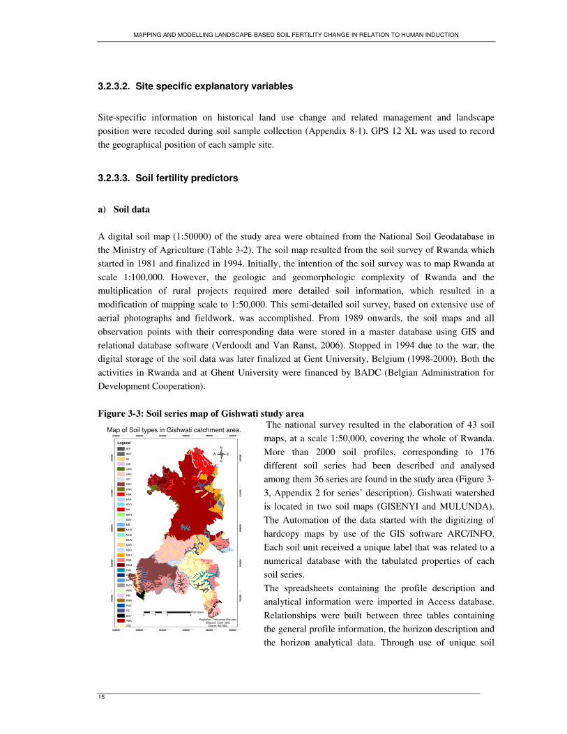
a) Soil data A digital soil map (1:50000) of the study area were obtained from the National Soil Geodatabase in the Ministry of Agriculture (Table 3-2). The soil map resulted from the soil survey of Rwanda which started in 1981 and finalized in 1994. Initially, the intention of the soil survey was to map Rwanda at scale 1:100,000. However, the geologic and geomorphologic complexity of Rwanda and the multiplication of rural projects required more detailed soil information, which resulted in a modification of mapping scale to 1:50,000. This semi-detailed soil survey, based on extensive use of aerial photographs and fieldwork, was accomplished. From 1989 onwards, the soil maps and all observation points with their corresponding data were stored in a master database using GIS and relational database software (Verdoodt and Van Ranst, 2006). Stopped in 1994 due to the war, the digital storage of the soil data was later finalized at Gent University, Belgium (1998-2000). Both the activities in Rwanda and at Ghent University were financed by BADC (Belgian Administration for Development Cooperation). Figure 3-3: Soil series map of Gishwati study area
The national survey resulted in the elaboration of 43 soil maps, at a scale 1:50,000, covering the whole of Rwanda. More than 2000 soil profiles, corresponding to 176 different soil series had been described and analysed among them 36 series are found in the study area (Figure 3-3, Appendix 2 for series’ description). Gishwati watershed is located in two soil maps (GISENYI and MULUNDA). The Automation of the data started with the digitizing of hardcopy maps by use of the GIS software ARC/INFO. Each soil unit received a unique label that was related to a numerical database with the tabulated properties of each soil series. The spreadsheets containing the profile description and analytical information were imported in Access database. Relationships were built between three tables containing the general profile information, the horizon description and the horizon analytical data. Through use of unique soil
424000.000000
424000.000000
428000.000000
428000.000000
432000.000000
432000.000000
436000.000000
436000.000000
440000.000000
440000.000000
444000.000000
444000.000000
7960
00.0
0000
0
7960
00.0
0000
0
8020
00.0
0000
0
8020
00.0
0000
0
8080
00.0
0000
0
8080
00.0
0000
0
8140
00.0
0000
0
8140
00.0
0000
0
8200
00.0
0000
0
8200
00.0
0000
0
LegendBRI
BWI
GI
GIR
GKB
GKK
GO
GSV
HNK
HSA
KAR
KRO
MA
MAH
MAY
MB
MHR
MUE
MUK
NAR
NBO
NBU
RAB
RAM
RAV
RH
RK
RKO
RKR
RM
RNB
RUE
RZ
SOV
TMA
TRE
0 4 82Kilometers
�
Map of Soil types in Gishwati catchment area.
Projection: Transverse MercatorEllipsoid: Clark 1880
Datum: Arc1960
MAPPING AND MODELLING LANDSCAPE-BASED SOIL FERTILITY CHANGE IN RELATION TO HUMAN INDUCTION
16
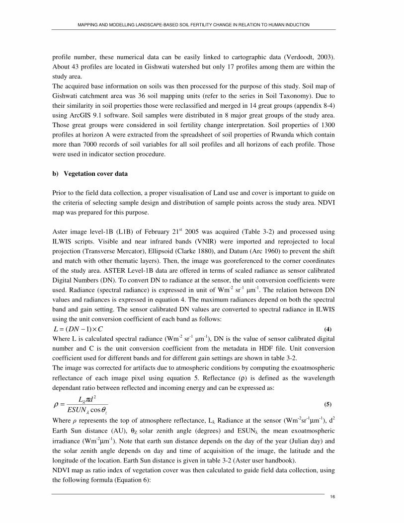
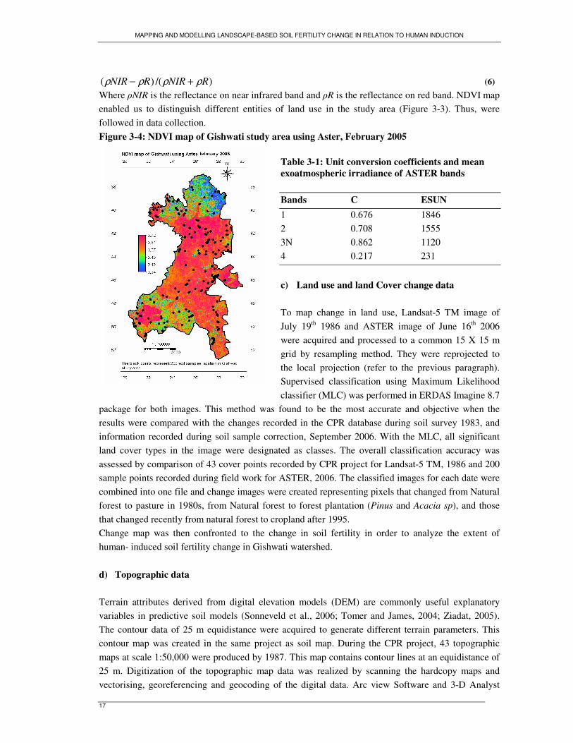
profile number, these numerical data can be easily linked to cartographic data (Verdoodt, 2003). About 43 profiles are located in Gishwati watershed but only 17 profiles among them are within the study area. The acquired base information on soils was then processed for the purpose of this study. Soil map of Gishwati catchment area was 36 soil mapping units (refer to the series in Soil Taxonomy). Due to their similarity in soil properties those were reclassified and merged in 14 great groups (appendix 8-4) using ArcGIS 9.1 software. Soil samples were distributed in 8 major great groups of the study area. Those great groups were considered in soil fertility change interpretation. Soil properties of 1300 profiles at horizon A were extracted from the spreadsheet of soil properties of Rwanda which contain more than 7000 records of soil variables for all soil profiles and all horizons of each profile. Those were used in indicator section procedure. b) Vegetation cover data Prior to the field data collection, a proper visualisation of Land use and cover is important to guide on the criteria of selecting sample design and distribution of sample points across the study area. NDVI map was prepared for this purpose. Aster image level-1B (L1B) of February 21st 2005 was acquired (Table 3-2) and processed using ILWIS scripts. Visible and near infrared bands (VNIR) were imported and reprojected to local projection (Transverse Mercator), Ellipsoid (Clarke 1880), and Datum (Arc 1960) to prevent the shift and match with other thematic layers). Then, the image was georeferenced to the corner coordinates of the study area. ASTER Level-1B data are offered in terms of scaled radiance as sensor calibrated Digital Numbers (DN). To convert DN to radiance at the sensor, the unit conversion coefficients were used. Radiance (spectral radiance) is expressed in unit of Wm-2 sr-1 �m-1. The relation between DN values and radiances is expressed in equation 4. The maximum radiances depend on both the spectral band and gain setting. The sensor calibrated DN values are converted to spectral radiance in ILWIS using the unit conversion coefficient of each band as follows:
CDNL ×−= )1( (4) Where L is calculated spectral radiance (Wm-2 sr-1 �m-1), DN is the value of sensor calibrated digital number and C is the unit conversion coefficient from the metadata in HDF file. Unit conversion coefficient used for different bands and for different gain settings are shown in table 3-2. The image was corrected for artifacts due to atmospheric conditions by computing the exoatmospheric reflectance of each image pixel using equation 5. Reflectance (ρ) is defined as the wavelength dependant ratio between reflected and incoming energy and can be expressed as:
zESUNdL
θπρλ
λ
cos
2
= (5)
Where � represents the top of atmosphere reflectance, Lλ Radiance at the sensor (Wm-2sr-1µm-1), d2 Earth Sun distance (AU), θZ solar zenith angle (degrees) and ESUNλ the mean exoatmospheric irradiance (Wm-2µm-1). Note that earth sun distance depends on the day of the year (Julian day) and the solar zenith angle depends on day and time of acquisition of the image, the latitude and the longitude of the location. Earth Sun distance is given in table 3-2 (Aster user handbook). NDVI map as ratio index of vegetation cover was then calculated to guide field data collection, using the following formula (Equation 6):
MAPPING AND MODELLING LANDSCAPE-BASED SOIL FERTILITY CHANGE IN RELATION TO HUMAN INDUCTION
17
)/()( RNIRRNIR ρρρρ +− (6) Where �NIR is the reflectance on near infrared band and �R is the reflectance on red band. NDVI map enabled us to distinguish different entities of land use in the study area (Figure 3-3). Thus, were followed in data collection. Figure 3-4: NDVI map of Gishwati study area using Aster, February 2005
Table 3-1: Unit conversion coefficients and mean exoatmospheric irradiance of ASTER bands
Bands C ESUN 1 0.676 1846 2 0.708 1555 3N 0.862 1120 4 0.217 231
c) Land use and land Cover change data To map change in land use, Landsat-5 TM image of July 19th 1986 and ASTER image of June 16th 2006 were acquired and processed to a common 15 X 15 m grid by resampling method. They were reprojected to the local projection (refer to the previous paragraph). Supervised classification using Maximum Likelihood classifier (MLC) was performed in ERDAS Imagine 8.7
package for both images. This method was found to be the most accurate and objective when the results were compared with the changes recorded in the CPR database during soil survey 1983, and information recorded during soil sample correction, September 2006. With the MLC, all significant land cover types in the image were designated as classes. The overall classification accuracy was assessed by comparison of 43 cover points recorded by CPR project for Landsat-5 TM, 1986 and 200 sample points recorded during field work for ASTER, 2006. The classified images for each date were combined into one file and change images were created representing pixels that changed from Natural forest to pasture in 1980s, from Natural forest to forest plantation (Pinus and Acacia sp), and those that changed recently from natural forest to cropland after 1995. Change map was then confronted to the change in soil fertility in order to analyze the extent of human- induced soil fertility change in Gishwati watershed. d) Topographic data Terrain attributes derived from digital elevation models (DEM) are commonly useful explanatory variables in predictive soil models (Sonneveld et al., 2006; Tomer and James, 2004; Ziadat, 2005). The contour data of 25 m equidistance were acquired to generate different terrain parameters. This contour map was created in the same project as soil map. During the CPR project, 43 topographic maps at scale 1:50,000 were produced by 1987. This map contains contour lines at an equidistance of 25 m. Digitization of the topographic map data was realized by scanning the hardcopy maps and vectorising, georeferencing and geocoding of the digital data. Arc view Software and 3-D Analyst
MAPPING AND MODELLING LANDSCAPE-BASED SOIL FERTILITY CHANGE IN RELATION TO HUMAN INDUCTION
18
extension ware used to derive a digital terrain model (DTM) for each map sheet (Verdoodt, 2003). The river network and spot heights of the study area were also supplied in the same Geo-database. Prior to the calculation of terrain parameters, the quality DEM was improved using the method proposed by Hengl et al., 2004 (Hengl et al., 2004a). This procedure is done to account for the features that are not shown by the contours such as ridges and valley bottom. The spot heights were assigned to the medial axis between the closed contours and the river networks were used to adjust the final DEM. The sinks were also filled. All these steps are well explained in terrain analysis user guide (Hengl et al., 2003). The improved DEM was then used to generate the relief parameters for soil landscape modelling. The contour was rasterized using a common grid (15x15m) of all variables involved in this study. This was used to generate Digital Elevation Map (DEM) and terrain attributes such as slope gradient (S=tan �, percent), specific catchment area (As, m2 m−1), topographic wetness index (TWI), stream power index (SPI) and Sediment transport index (STI). The topographic wetness index, a predictor of zones of soil saturation, is the ratio of specific catchment area to slope gradient:
)/ln( SAsTWI = . (7) The stream power index, a measure of runoff erosivity, is the product of specific catchment area and slope gradient:
)ln( SAsSPI ×= . (8) The sediment transport index, also called erosion index is modelled as following:
3.16.0 )0896.0/(sin)13.22/( β×= ASSTI . (9) For detail elaborations refer to (Hengl et al., 2003; Thompson et al., 2006; Tomer and James, 2004). The calculations were performed using flow indices script in ILWIS 3.0. Table 3-2: Data type and key variables considered for soil fertility change analysis Data type variables Source Initial Soil fertility indicators (before deforestation)(1:50,000)
pHw, pHKCl avail.P, OC, Exch. bases (Ca, Mg, K), Echange acidity (Al, H).
Soil Geo-database of Rwanda MINAGRI (Kigali/Rwanda)
Actual MSFI (2006) pHw, pHKCl, avail.P, OC, Exch. bases (Ca, Mg, K), Exch. acidity (Al, H).
Primary data Soil measurements
Soil type Soil series and related variables
Soil Geo-database of Rwanda MINAGRI (Kigali/Rwanda)
Topographic data (1:50,000)
Contour data (25 m equidistance) Spot heights and River network DEM, derived Terrains parameters
Soil Geo-database of Rwanda MINAGRI (Kigali/ Rwanda)
Interviews and Field observation
Historical land uses and related management Erosion features
Site-specific information (smallholder farmers and local operators: ISAR/Gishwati, PAFOR).
Remote Sensing data Landsat-5 TM 16th July 1986, ASTER 21st January, 2005 and 21st June 2006
Land use / cover types Vegetation index (NDVI)
Geodata Warehouse (ITC Enschede)
MAPPING AND MODELLING LANDSCAPE-BASED SOIL FERTILITY CHANGE IN RELATION TO HUMAN INDUCTION
19
3.2.4. Soil fertility change analysis
3.2.4.1. Selection of the Minimum soil fertility indicators (MSFI)
Due to the limited logistic and time, the study of soil fertility as the combination of various soil properties that determine the capacity of the soil to crop production function, started by reducing the soil variables prior to data collection and laboratory activities. This lead to a minimum data set for soil fertility assessment in Gishwati catchment area. The MSFI should just be considered as the smallest set of the soil chemical properties that can best represent the human-induced change in soil fertility. This approach is similar to the Minimum Data Set (MDS) approach (Park and Vlek, 2002; Yemefack et al., 2006), the only difference is that the MSFI is limited to the chemical soil properties whereas the MDS consider both physical and chemical properties i.e. the MSFI is part of the MDS. We agree with different researchers that the soil chemical properties to be included in a MSFI must be sensitive to changes in soil management, soil perturbations, and inputs into the soil system. (McBratney et al., 2003; Sena et al., 2002; Yemefack, 2005; Yemefack et al., 2006; Yemefack et al., 2005). Each selected property must also be inexpensively, easily and reproducibly measurable. Reducing the redundancy between soil chemical variables was achieved by evaluating the correlation of variables over the whole dataset of Rwanda. The Spearman correlation was computed on the multivariate data matrix using 1300 soil samples collected and analyzed during the semi-detailed soil survey of 1981. This non-parametric method was used to avoid distortions from non-normally distributed variables or extreme values (Yemefack, 2005). To cross-check the result of this correlation analysis, Principal Component Analysis (PCA) was also performed as one of factor analysis for soil variables reductions. Properties that had high score of PCA value and highly correlated were classified in one group. The included soil variable in the MSFI was defined to be the highest scored variable in PCA and sometimes times with less correlation among themselves.
3.2.4.2. Sampling design
Refer to the distribution of human activities in Gishwati study area, such as the division of the land into different land uses (Figure 3-3), we realised that there were organized control. As result, the human-induced soil fertility change can not be random, except within the same use, same soil and same landscape position. This situation leads us to the stratified sampling design. We agree also with soil conservation scientist that simulated erosion patterns and nutrient losses are directly related to the flow network of the catchment. Since the model routes water and suspended sediment towards the outlet using a user-supplied network (Jetten et al., 2003), the flow of soil nutrients is closely related to this network. Therefore, stratified toposequence transect sampling seemed to be appropriate and transect location was chosen purposely. About 67 toposequential transect locations were chosen to represent major Land Use classes with different topography and soil types. Each transect included at least three of five separate sampling points collected at summit, upper slope, middle slope, lower slope, and valley.
MAPPING AND MODELLING LANDSCAPE-BASED SOIL FERTILITY CHANGE IN RELATION TO HUMAN INDUCTION
20
3.2.4.3. Soil sample collection and laboratory analysis
Nutrients in soil solution are readily plant-available. In that case, topsoil properties may be used as an indication of nutrient availability to plants because most roots are concentrated in the A horizons (Lilienfein et al., 2003). Soil samples were collected from Gishwati catchment area by augering at 0-30 cm depth. These were analysed in the PASI laboratory, Faculty of Agriculture at the National University of Rwanda (NUR) for the following determinations: pH water and pHKCl with a ratio of 1:2.5 (pHw), organic carbon (Org.C) using the Walkley-Black method, available P (avail.P) using the Bray-1 method, exchangeable bases (exch.B) using the ammonium acetate percolation method, exchange acidity (Exch. Ac.) using an unbuffered KCl solution. All these methods are described in (ABOS-AGCD, 1983). The same methods were used to analyze the soil chemical properties in CPR project.
3.2.4.4. Relations of soil fertility to predictive factors
One-way analyses of variance (ANOVAs) were performed on each soil fertility indicator per Soil type, Type of change in land use and landscape positions to test whether, the relations investigated were statistically significant. Mean values were compared using Duncan test. Duncan test separates the means of soil fertility indicator variables at α =0.05.
3.2.5. Soil fertility change interpretation
3.2.5.1. Development of soil fertility index (SFI)
The development of an integrative index of soil fertility (SFI) was utmost important to capture the variability of individual indicator of soil fertility. Once we had the most dynamic soil variables, the next task was to integrate them into a value that indicates at once the maximum variability both in space and time. This index gives an explicit indication of soil fertility that can not be easily seen using each soil property. Probabilistic model are becoming increasingly important in analyzing the huge amount of data being produced by different scale, methods or different laboratory analysis. The integration involved transformation of each observed MSFI value in scored value (probability value) using thresholds for interpretation of topsoil properties of Rwanda (Appendix 11, 12, 13). This method assumes that the indicator is measured according to the standard method for near surface (0-30 cm) (Mutwewingabo et Rutunga, 1987), and that sampling design was appropriate for the area to be assessed (Andrews et al., 2004). The conceptual model (Figure 3-5) summarizes the steps for soil fertility index development (SFID). In this framework, measured MSFI values were transformed into unitless score (0 to 1) using thresholds of soil properties classes of Rwanda and probabilistic approach. Each soil fertility indicator was assigned its probability that it falls into very high fertile soil. An indicator score of 1 represent
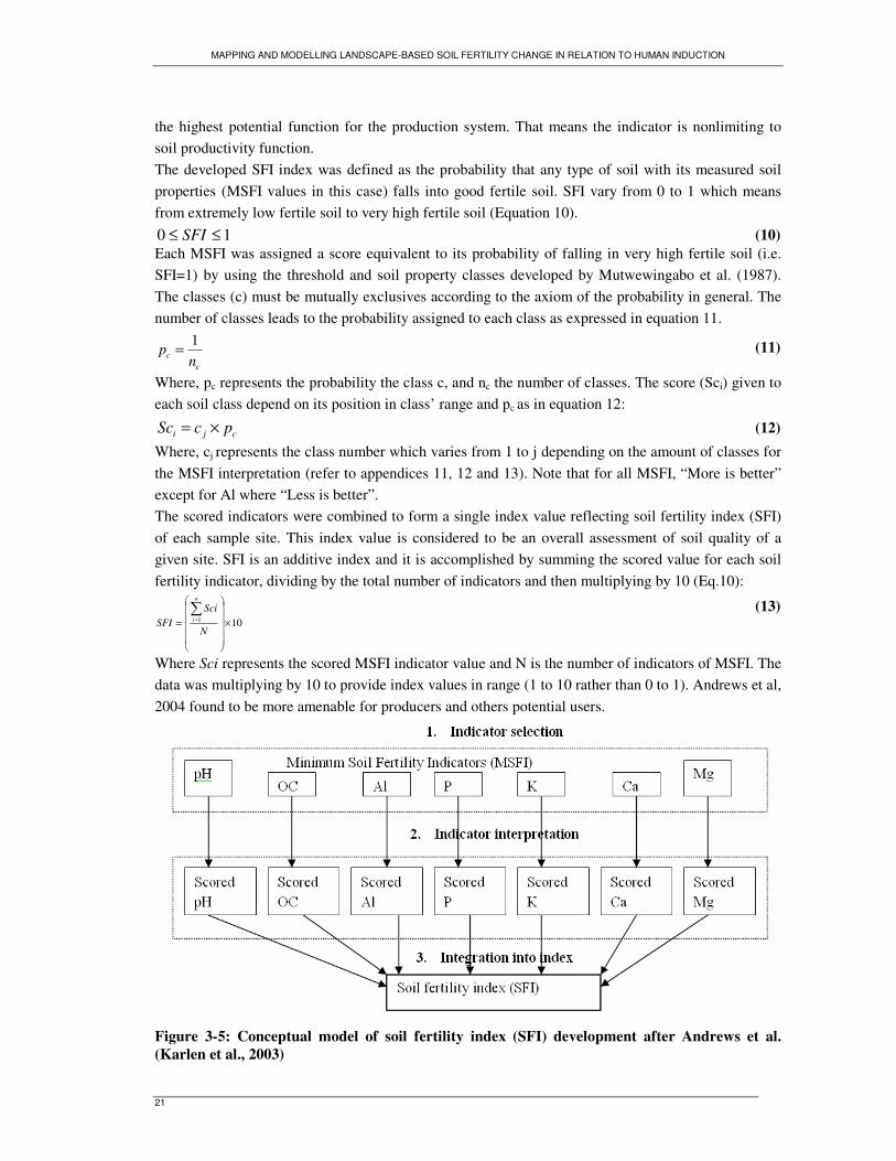
MAPPING AND MODELLING LANDSCAPE-BASED SOIL FERTILITY CHANGE IN RELATION TO HUMAN INDUCTION
21
the highest potential function for the production system. That means the indicator is nonlimiting to soil productivity function. The developed SFI index was defined as the probability that any type of soil with its measured soil properties (MSFI values in this case) falls into good fertile soil. SFI vary from 0 to 1 which means from extremely low fertile soil to very high fertile soil (Equation 10).
10 ≤≤ SFI (10) Each MSFI was assigned a score equivalent to its probability of falling in very high fertile soil (i.e. SFI=1) by using the threshold and soil property classes developed by Mutwewingabo et al. (1987). The classes (c) must be mutually exclusives according to the axiom of the probability in general. The number of classes leads to the probability assigned to each class as expressed in equation 11.
cc n
p1= (11)
Where, pc represents the probability the class c, and nc the number of classes. The score (Sci) given to each soil class depend on its position in class’ range and pc as in equation 12:
cji pcSc ×= (12) Where, cj represents the class number which varies from 1 to j depending on the amount of classes for the MSFI interpretation (refer to appendices 11, 12 and 13). Note that for all MSFI, “More is better” except for Al where “Less is better”. The scored indicators were combined to form a single index value reflecting soil fertility index (SFI) of each sample site. This index value is considered to be an overall assessment of soil quality of a given site. SFI is an additive index and it is accomplished by summing the scored value for each soil fertility indicator, dividing by the total number of indicators and then multiplying by 10 (Eq.10):
101 ����
�
�
����
�
�
=�
=
N
SciSFI
n
i
(13)
Where Sci represents the scored MSFI indicator value and N is the number of indicators of MSFI. The data was multiplying by 10 to provide index values in range (1 to 10 rather than 0 to 1). Andrews et al, 2004 found to be more amenable for producers and others potential users.
Figure 3-5: Conceptual model of soil fertility index (SFI) development after Andrews et al. (Karlen et al., 2003)
MAPPING AND MODELLING LANDSCAPE-BASED SOIL FERTILITY CHANGE IN RELATION TO HUMAN INDUCTION
22
3.2.5.2. Index of Soil fertility deterioration (DI)
After that SFI was determined for each sample point, the soil deterioration index (DI) was computed on the assumption that the status of soil fertility under pine plantation, pasture and agriculture were once the same as that of adjacent soil under natural forest prior to conversion. The difference between each value of SFI under pine plantation, pasture and agriculture were compared to baseline mean value of SFI under natural forest. The deterioration index (DI) was calculated as deviation of SFI values from SFI of Natural forest (SFINF) to other land cover type (SFILCi) under a specific soil type. Eutrandepts were used as one of representative soil type in Gishwati study area.
NFLC SFISFIDIi
−= (14)
3.2.5.3. Geostatistical analysis
The development of the cross variogram model for soil fertility might be very beneficial for Gishwati study area if prediction is sufficiently accurate. For instance in Agriculture, the predicted map from developed SFI model might be a tool for monitoring and implementing site specific management. Secondly, in management goal, SFI define at once the situation that happened instead of what happened to individual parameter which could be difficult to understand because sometimes they contradict each other. In this case SFI average the behaviour of its predictors into a common behaviour of soil fertility across the study area. 1) Spatial prediction of SFI using smoothing Kriging (OK) Kriging is one of interpolation techniques that use spatial correlation between observation points. With OK, the trend is modelled as a function of the location (Hengl et al., 2004b). There are a number of considerations in geostatistical analysis including normality, anisotropy, and semivariogram model selection. While normality is not a requirement for developing the semivariogram or kriging, the classical linear Kriging predictor (i. e. OK in this case) is not the best predictor if the spatial process is not Gaussian (Mueller et al., 2001). The interpolation of target variable (in this case SFI) is based on assumption that the original process is a diffusion process (Lark and Ferguson, 2004; Webster, 2000). It varies continuously so that if the target variable takes values zj and zi at locations xi and xj, respectively, then all intervening values between these two must occur at locations between xi and xj. The commonest model, which we used for Kriging, is the Gaussian diffusion process. Since SFI data more or less resembled to Gaussian distribution, the nonlinear transform to achieve normality was not necessary. A variogram is estimated using Matheron’s estimator (1965).
{ }2
1
)()(2
1)( �
=
∧+−=
hM
iii
h
hxzxzM
hγ (15)
Where, Z (xi) is the property value (SFI in this case) at a given location (xi), h is lag (both distance and direction), Mh is the pairs of observation points, separated by h; and �ˆ (h) is semi-variance at lag h. Kriging assumes a certain degree of spatial correlation between the input point values. To investigate whether SFI values were spatially correlated and until which distance from any point this correlation occurs, we used the Spatial Correlation operation in ILWIS. This distance value was then used for the limiting distance in point interpolations using OK.
MAPPING AND MODELLING LANDSCAPE-BASED SOIL FERTILITY CHANGE IN RELATION TO HUMAN INDUCTION
23
2) Spatial prediction using Kriging with ancillary variables SFI pair points may be correlated because they are affected by similar processes, or phenomena, that extend over a larger area. For instance they may correlate because they are under similar land use or under the same soil type. In this case, a mixed approach is used to explain what can be explained by knowledge of soil-forming factors (as expressed in CLORPT model), and then see if the remaining unexplained variability has any geostatistical relation which can be used to improve the prediction. Regression Kriging (RK) or Kriging with External Drift (KED) use a CLORPT variable as predictor of soil attribute. However, both KED and RK has the same mathematical form and yields the same predictions (Hengl et al., 2004b). The impact of soil type, land use change and landscape on soil fertility variation in the study area were investigated using analysis of variance procedures. Most of the soil fertility variables varied between soil types, type of change in land uses and landscape positions. Therefore, the interpolation involved them in the model of SFI trend by using stepwise regression procedures and the residuals were extracted and fitted in geostatistical model. We used DEM, Slope gradient (S), Topographic Wetness Index (TWI), Stream Power Index (SPI) and Sediment Transport Index (STI) as predictors. They were first linearly stretched to a range of 0-255 to give each map equal contrast. To account for multicollinearity, a factor analysis prior to regression analysis was applied to produce the soil predictive components (SPCs) using ILWIS. The use of standardised principal component instead of the original terrain variable improves the prediction for soil-landscape modelling (Hengl et al., 2004b). The SPCs values were then extracted for SFI locations for the stepwise regression modelling. The regression model of SFI as function of SPCs was then generated. SFI Point data were imported to an ILWIS table with XY and SFI coordinates. We first estimated the values of predictors (SPCs) at the measured SFI locations and we fitted the trend (SFI trend) by using an obtained regression model. Secondary, we estimated the residuals at sampled locations using: SFI residual as difference between measured SFI and SFI trend using ‘SFI-MapValue (SFI trend, Coordinate)’ syntax. Third, Gaussian variogram model of SFI residual was fitted and SFI residual was interpolated using OK (interpolated SFI residual). The fitted trend and residuals was then added back together using ‘predicted SFI=SFI trend +interpolated SFI residual’. All those calculation was done using ILWIS command line (for detail refer to http://spatial-analyst.net/RKguide.php). To improve the SFI prediction, SMUs was used to stratify SPCs in Stepwise regression by using WLS. This technique adds the contribution of soil type on SFI to SPCs explanation. Then RK proceeded in ILWIS as described in previous paragraph. 3) Spatial prediction of soil fertility deterioration over 25 years The spatial distribution of soil fertility deterioration index (DI) was computed as deviation of SFI from SFI before deforestation to the current situation of soil fertility. In this case Type I method is made possible through the predicted maps because it gives on opportunity to monitor the change in soil fertility at a given location. This deterioration reflects the human-induced soil fertility loss in Gishwati study area and it is expressed as in equation 16:
if tyxtyxyxtyx SFISFItSFIfDI ),(),(),(),( ),( −== (16)
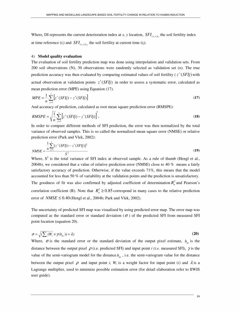
MAPPING AND MODELLING LANDSCAPE-BASED SOIL FERTILITY CHANGE IN RELATION TO HUMAN INDUCTION
24
Where, DI represents the current deterioration index at x, y location, itysSFI ),( the soil fertility index
at time reference (ti) and ftysSFI ),( the soil fertility at current time (tf).
4) Model quality evaluation The evaluation of soil fertility prediction map was done using interpolation and validation sets. From 200 soil observations (N), 30 observations were randomly selected as validation set (n). The true
prediction accuracy was then evaluated by comparing estimated values of soil fertility ( )(SFIjz∧ with
actual observation at validation points )(SFIjz∗ in order to assess a systematic error, calculated as
mean prediction error (MPE) using Equation (17).
[ ]�=
∗∧ −=1
1
)()(.1
j
SFIjzSFIjzn
MPE (17)
And accuracy of prediction, calculated as root mean square prediction error (RMSPE):
[ ]21
1
)()(.1�
=
∗∧ −=j
SFIjzSFIjzn
RMSPE . (18)
In order to compare different methods of SFI prediction, the error was then normalized by the total variance of observed samples. This is so called the normalized mean square error (NMSE) or relative prediction error (Park and Vlek, 2002):
2
1
1
2)]()([1
S
SFIjzSFIjzn
NMSE j�
=
∗∧ −= (19)
Where, S2 is the total variance of SFI index at observed sample. As a rule of thumb (Hengl et al., 2004b), we considered that a value of relative prediction error (NMSE) close to 40 % means a fairly satisfactory accuracy of prediction. Otherwise, if the value exceeds 71%, this means that the model accounted for less than 50 % of variability at the validation points and the prediction is unsatisfactory.
The goodness of fit was also confirmed by adjusted coefficient of determination 2aR and Pearson’s
correlation coefficient (R). Note that 85.02 ≥aR correspond in many cases to the relative prediction
error of 40.0≤NMSE (Hengl et al., 2004b; Park and Vlek, 2002). The uncertainty of predicted SFI map was visualized by using predicted error map. The error map was computed as the standard error or standard deviation (σ ) of the predicted SFI from measured SFI point location (equation 20).
)))((( λγσ ρ +×= � ihW
i i (20)
Where, σ is the standard error or the standard deviation of the output pixel estimate, i
hρ is the
distance between the output pixel ρ (i.e. predicted SFI) and input point i (i.e. measured SFI), γ is the
value of the semi-variogram model for the distancei
hρ , i.e. the semi-variogram value for the distance
between the output pixel ρ and input point i, Wi is a weight factor for input point (i) and λ is a
Lagrange multiplier, used to minimize possible estimation error (for detail elaboration refer to IlWIS user guide).
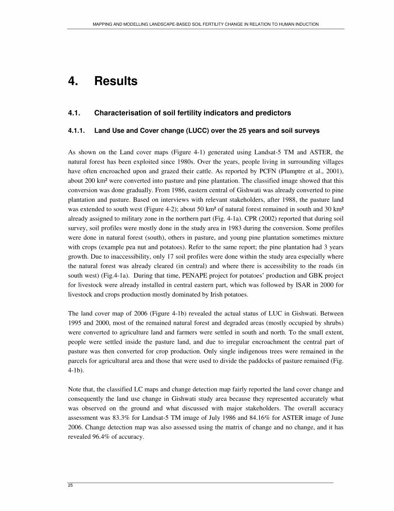
MAPPING AND MODELLING LANDSCAPE-BASED SOIL FERTILITY CHANGE IN RELATION TO HUMAN INDUCTION
25
4. Results
4.1. Characterisation of soil fertility indicators and predictors
4.1.1. Land Use and Cover change (LUCC) over the 25 years and soil surveys
As shown on the Land cover maps (Figure 4-1) generated using Landsat-5 TM and ASTER, the natural forest has been exploited since 1980s. Over the years, people living in surrounding villages have often encroached upon and grazed their cattle. As reported by PCFN (Plumptre et al., 2001), about 200 km² were converted into pasture and pine plantation. The classified image showed that this conversion was done gradually. From 1986, eastern central of Gishwati was already converted to pine plantation and pasture. Based on interviews with relevant stakeholders, after 1988, the pasture land was extended to south west (Figure 4-2); about 50 km² of natural forest remained in south and 30 km² already assigned to military zone in the northern part (Fig. 4-1a). CPR (2002) reported that during soil survey, soil profiles were mostly done in the study area in 1983 during the conversion. Some profiles were done in natural forest (south), others in pasture, and young pine plantation sometimes mixture with crops (example pea nut and potatoes). Refer to the same report; the pine plantation had 3 years growth. Due to inaccessibility, only 17 soil profiles were done within the study area especially where the natural forest was already cleared (in central) and where there is accessibility to the roads (in south west) (Fig.4-1a). During that time, PENAPE project for potatoes’ production and GBK project for livestock were already installed in central eastern part, which was followed by ISAR in 2000 for livestock and crops production mostly dominated by Irish potatoes. The land cover map of 2006 (Figure 4-1b) revealed the actual status of LUC in Gishwati. Between 1995 and 2000, most of the remained natural forest and degraded areas (mostly occupied by shrubs) were converted to agriculture land and farmers were settled in south and north. To the small extent, people were settled inside the pasture land, and due to irregular encroachment the central part of pasture was then converted for crop production. Only single indigenous trees were remained in the parcels for agricultural area and those that were used to divide the paddocks of pasture remained (Fig. 4-1b). Note that, the classified LC maps and change detection map fairly reported the land cover change and consequently the land use change in Gishwati study area because they represented accurately what was observed on the ground and what discussed with major stakeholders. The overall accuracy assessment was 83.3% for Landsat-5 TM image of July 1986 and 84.16% for ASTER image of June 2006. Change detection map was also assessed using the matrix of change and no change, and it has revealed 96.4% of accuracy.
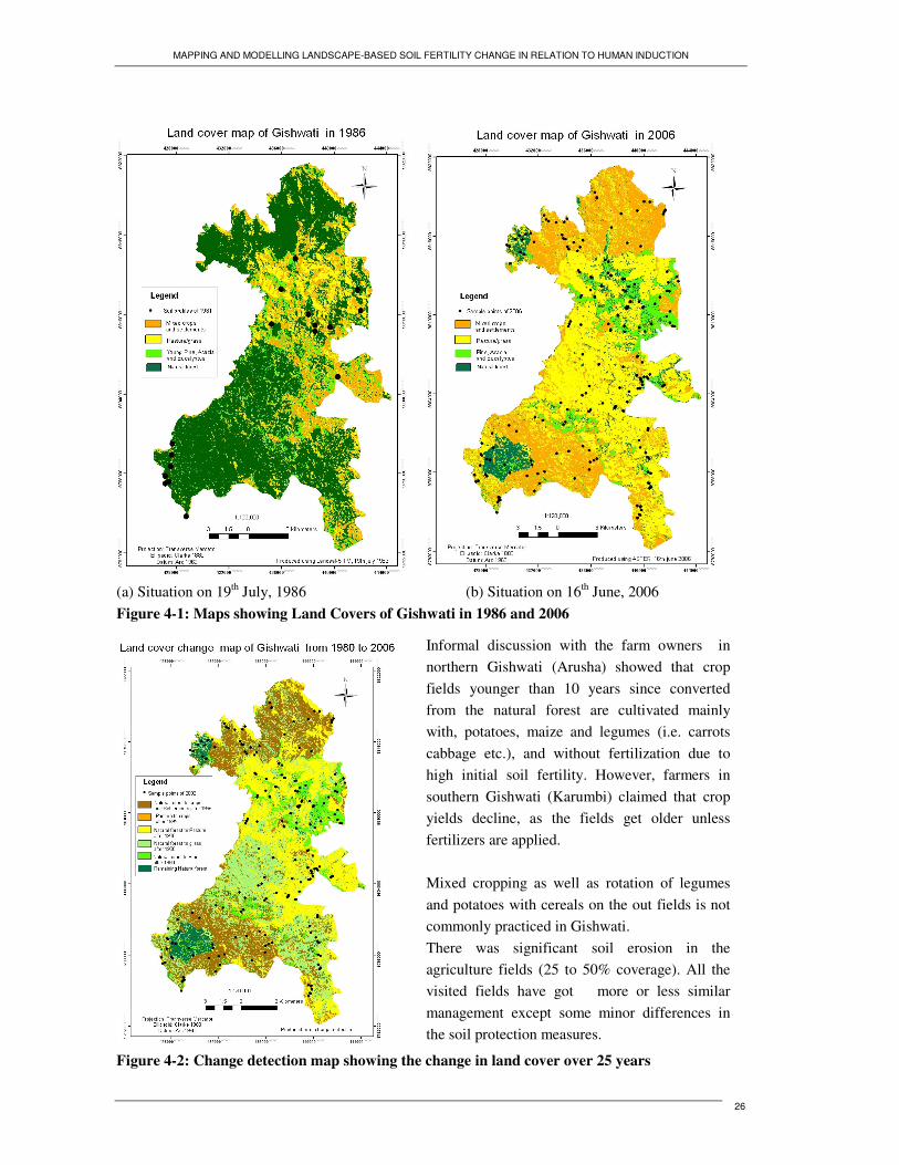
MAPPING AND MODELLING LANDSCAPE-BASED SOIL FERTILITY CHANGE IN RELATION TO HUMAN INDUCTION
26
(a) Situation on 19th July, 1986 (b) Situation on 16th June, 2006 Figure 4-1: Maps showing Land Covers of Gishwati in 1986 and 2006
Figure 4-2: Change detection map showing the change in land cover over 25 years
Informal discussion with the farm owners in northern Gishwati (Arusha) showed that crop fields younger than 10 years since converted from the natural forest are cultivated mainly with, potatoes, maize and legumes (i.e. carrots cabbage etc.), and without fertilization due to high initial soil fertility. However, farmers in southern Gishwati (Karumbi) claimed that crop yields decline, as the fields get older unless fertilizers are applied. Mixed cropping as well as rotation of legumes and potatoes with cereals on the out fields is not commonly practiced in Gishwati. There was significant soil erosion in the agriculture fields (25 to 50% coverage). All the visited fields have got more or less similar management except some minor differences in the soil protection measures.
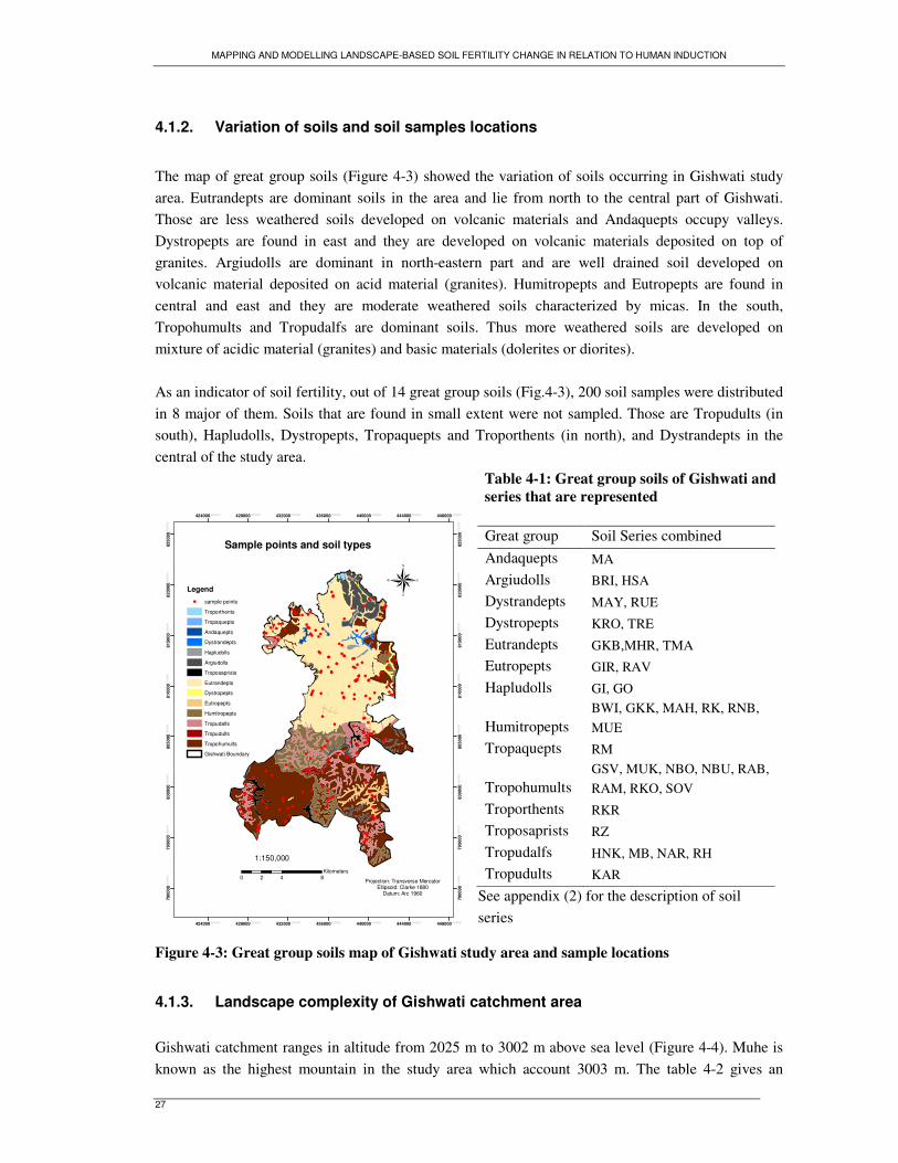
MAPPING AND MODELLING LANDSCAPE-BASED SOIL FERTILITY CHANGE IN RELATION TO HUMAN INDUCTION
27
4.1.2. Variation of soils and soil samples locations
The map of great group soils (Figure 4-3) showed the variation of soils occurring in Gishwati study area. Eutrandepts are dominant soils in the area and lie from north to the central part of Gishwati. Those are less weathered soils developed on volcanic materials and Andaquepts occupy valleys. Dystropepts are found in east and they are developed on volcanic materials deposited on top of granites. Argiudolls are dominant in north-eastern part and are well drained soil developed on volcanic material deposited on acid material (granites). Humitropepts and Eutropepts are found in central and east and they are moderate weathered soils characterized by micas. In the south, Tropohumults and Tropudalfs are dominant soils. Thus more weathered soils are developed on mixture of acidic material (granites) and basic materials (dolerites or diorites). As an indicator of soil fertility, out of 14 great group soils (Fig.4-3), 200 soil samples were distributed in 8 major of them. Soils that are found in small extent were not sampled. Those are Tropudults (in south), Hapludolls, Dystropepts, Tropaquepts and Troporthents (in north), and Dystrandepts in the central of the study area.
Table 4-1: Great group soils of Gishwati and series that are represented
�
�����
��
�
�
�
���
�
�
�
�
�
�
��
� �
���
��
��
��
���
��
�
�����
��
�
��
��
��
��
���
�
��
��
��
����
�
�
��
����
��
�
�
���
� �
�
�
��
����
���
�
���
��
��
���
�
�
��
�
���
��
��
���
�
�
��
�
��
�
��
�
�
�
�
�
��
�
�
�
�
�
�
�
�
�
�
�
�
�
��
��
�
���
�
�
�
��
�
��
��
��� � �
�
��
�
� �
�
�
�
�
�
��
�
�
�
��
�
�
�
�
�
�
424000.000000
424000.000000
428000.000000
428000.000000
432000.000000
432000.000000
436000.000000
436000.000000
440000.000000
440000.000000
444000.000000
444000.000000
448000.000000
448000.000000
7900
00.0
0000
0
7900
00.0
0000
0
7950
00.0
0000
0
7950
00.0
0000
0
8000
00.0
0000
0
8000
00.0
0000
0
8050
00.0
0000
0
8050
00.0
0000
0
8100
00.0
0000
0
8100
00.0
0000
0
8150
00.0
0000
0
8150
00.0
0000
0
8200
00.0
0000
0
8200
00.0
0000
0
8250
00.0
0000
0
8250
00.0
0000
0
Sample points and soil types
Legend� sample points
Troporthents
Tropaquepts
Andaquepts
Dystrandepts
Hapludolls
Argiudolls
Troposaprists
Eutrandepts
Dystropepts
Eutropepts
Humitropepts
Tropudalfs
Tropudults
Tropohumults
Gishwati Boundary
1:150,000
0 4 82Kilometers
Projection: Transverse MercatorEllipsoid: Clarke 1880
Datum: Arc 1960
�
Figure 4-3: Great group soils map of Gishwati study area and sample locations
4.1.3. Landscape complexity of Gishwati catchment area
Gishwati catchment ranges in altitude from 2025 m to 3002 m above sea level (Figure 4-4). Muhe is known as the highest mountain in the study area which account 3003 m. The table 4-2 gives an
Great group Soil Series combined Andaquepts MA
Argiudolls BRI, HSA
Dystrandepts MAY, RUE
Dystropepts KRO, TRE
Eutrandepts GKB,MHR, TMA
Eutropepts GIR, RAV
Hapludolls GI, GO
Humitropepts BWI, GKK, MAH, RK, RNB, MUE
Tropaquepts RM
Tropohumults GSV, MUK, NBO, NBU, RAB, RAM, RKO, SOV
Troporthents RKR
Troposaprists RZ
Tropudalfs HNK, MB, NAR, RH
Tropudults KAR
See appendix (2) for the description of soil series
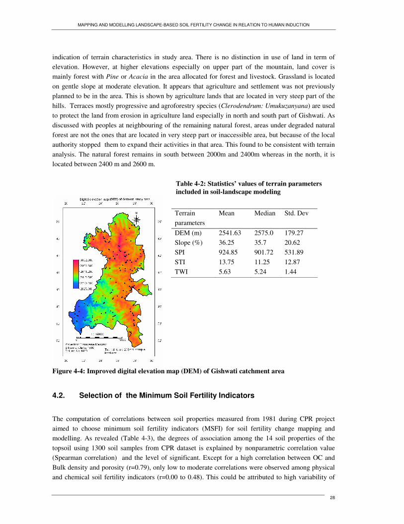
MAPPING AND MODELLING LANDSCAPE-BASED SOIL FERTILITY CHANGE IN RELATION TO HUMAN INDUCTION
28
indication of terrain characteristics in study area. There is no distinction in use of land in term of elevation. However, at higher elevations especially on upper part of the mountain, land cover is mainly forest with Pine or Acacia in the area allocated for forest and livestock. Grassland is located on gentle slope at moderate elevation. It appears that agriculture and settlement was not previously planned to be in the area. This is shown by agriculture lands that are located in very steep part of the hills. Terraces mostly progressive and agroforestry species (Clerodendrum: Umukuzanyana) are used to protect the land from erosion in agriculture land especially in north and south part of Gishwati. As discussed with peoples at neighbouring of the remaining natural forest, areas under degraded natural forest are not the ones that are located in very steep part or inaccessible area, but because of the local authority stopped them to expand their activities in that area. This found to be consistent with terrain analysis. The natural forest remains in south between 2000m and 2400m whereas in the north, it is located between 2400 m and 2600 m.
Table 4-2: Statistics’ values of terrain parameters included in soil-landscape modeling
Figure 4-4: Improved digital elevation map (DEM) of Gishwati catchment area
4.2. Selection of the Minimum Soil Fertility Indicators
The computation of correlations between soil properties measured from 1981 during CPR project aimed to choose minimum soil fertility indicators (MSFI) for soil fertility change mapping and modelling. As revealed (Table 4-3), the degrees of association among the 14 soil properties of the topsoil using 1300 soil samples from CPR dataset is explained by nonparametric correlation value (Spearman correlation) and the level of significant. Except for a high correlation between OC and Bulk density and porosity (r=0.79), only low to moderate correlations were observed among physical and chemical soil fertility indicators (r=0.00 to 0.48). This could be attributed to high variability of
Terrain parameters
Mean Median Std. Dev
DEM (m) 2541.63 2575.0 179.27 Slope (%) 36.25 35.7 20.62 SPI 924.85 901.72 531.89 STI 13.75 11.25 12.87 TWI 5.63 5.24 1.44
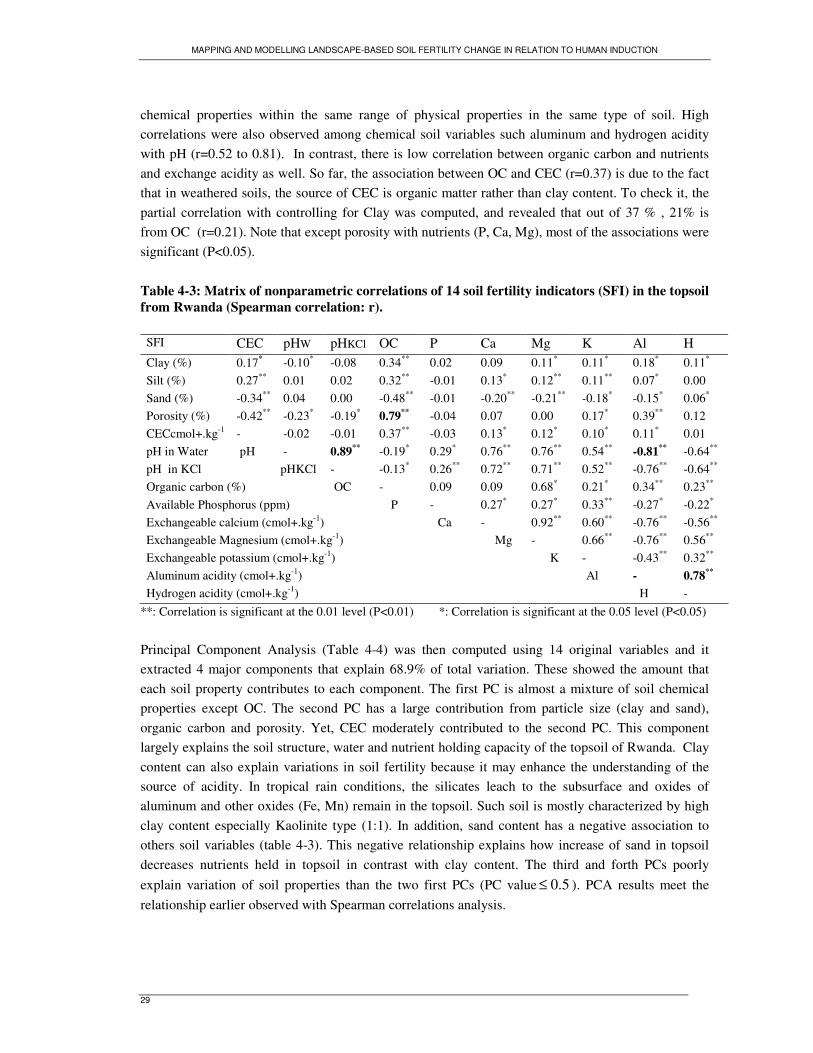
MAPPING AND MODELLING LANDSCAPE-BASED SOIL FERTILITY CHANGE IN RELATION TO HUMAN INDUCTION
29
chemical properties within the same range of physical properties in the same type of soil. High correlations were also observed among chemical soil variables such aluminum and hydrogen acidity with pH (r=0.52 to 0.81). In contrast, there is low correlation between organic carbon and nutrients and exchange acidity as well. So far, the association between OC and CEC (r=0.37) is due to the fact that in weathered soils, the source of CEC is organic matter rather than clay content. To check it, the partial correlation with controlling for Clay was computed, and revealed that out of 37 % , 21% is from OC (r=0.21). Note that except porosity with nutrients (P, Ca, Mg), most of the associations were significant (P<0.05). Table 4-3: Matrix of nonparametric correlations of 14 soil fertility indicators (SFI) in the topsoil from Rwanda (Spearman correlation: r). SFI CEC pHW pHKCl OC P Ca Mg K Al H Clay (%) 0.17* -0.10* -0.08 0.34** 0.02 0.09 0.11* 0.11* 0.18* 0.11* Silt (%) 0.27** 0.01 0.02 0.32** -0.01 0.13* 0.12** 0.11** 0.07* 0.00 Sand (%) -0.34** 0.04 0.00 -0.48** -0.01 -0.20** -0.21** -0.18* -0.15* 0.06* Porosity (%) -0.42** -0.23* -0.19* 0.79** -0.04 0.07 0.00 0.17* 0.39** 0.12 CECcmol+.kg-1 - -0.02 -0.01 0.37** -0.03 0.13* 0.12* 0.10* 0.11* 0.01 pH in Water pH - 0.89** -0.19* 0.29* 0.76** 0.76** 0.54** -0.81** -0.64** pH in KCl pHKCl - -0.13* 0.26** 0.72** 0.71** 0.52** -0.76** -0.64** Organic carbon (%) OC - 0.09 0.09 0.68* 0.21* 0.34** 0.23** Available Phosphorus (ppm) P - 0.27* 0.27* 0.33** -0.27* -0.22* Exchangeable calcium (cmol+.kg-1) Ca - 0.92** 0.60** -0.76** -0.56** Exchangeable Magnesium (cmol+.kg-1) Mg - 0.66** -0.76** 0.56** Exchangeable potassium (cmol+.kg-1) K - -0.43** 0.32** Aluminum acidity (cmol+.kg-1) Al - 0.78** Hydrogen acidity (cmol+.kg-1) H -
**: Correlation is significant at the 0.01 level (P<0.01) *: Correlation is significant at the 0.05 level (P<0.05)
Principal Component Analysis (Table 4-4) was then computed using 14 original variables and it extracted 4 major components that explain 68.9% of total variation. These showed the amount that each soil property contributes to each component. The first PC is almost a mixture of soil chemical properties except OC. The second PC has a large contribution from particle size (clay and sand), organic carbon and porosity. Yet, CEC moderately contributed to the second PC. This component largely explains the soil structure, water and nutrient holding capacity of the topsoil of Rwanda. Clay content can also explain variations in soil fertility because it may enhance the understanding of the source of acidity. In tropical rain conditions, the silicates leach to the subsurface and oxides of aluminum and other oxides (Fe, Mn) remain in the topsoil. Such soil is mostly characterized by high clay content especially Kaolinite type (1:1). In addition, sand content has a negative association to others soil variables (table 4-3). This negative relationship explains how increase of sand in topsoil decreases nutrients held in topsoil in contrast with clay content. The third and forth PCs poorly explain variation of soil properties than the two first PCs (PC value 5.0≤ ). PCA results meet the relationship earlier observed with Spearman correlations analysis.
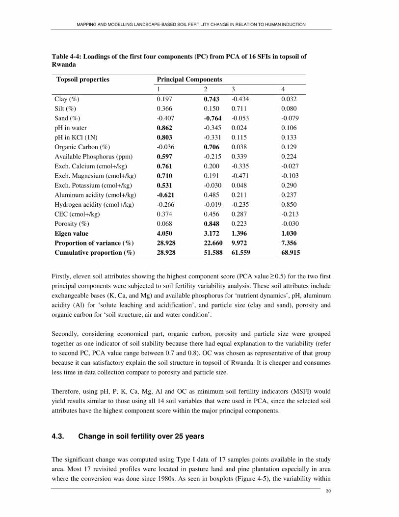
MAPPING AND MODELLING LANDSCAPE-BASED SOIL FERTILITY CHANGE IN RELATION TO HUMAN INDUCTION
30
Table 4-4: Loadings of the first four components (PC) from PCA of 16 SFIs in topsoil of Rwanda
Principal Components Topsoil properties 1 2 3 4 Clay (%) 0.197 0.743 -0.434 0.032 Silt (%) 0.366 0.150 0.711 0.080 Sand (%) -0.407 -0.764 -0.053 -0.079 pH in water 0.862 -0.345 0.024 0.106 pH in KCl (1N) 0.803 -0.331 0.115 0.133 Organic Carbon (%) -0.036 0.706 0.038 0.129 Available Phosphorus (ppm) 0.597 -0.215 0.339 0.224 Exch. Calcium (cmol+/kg) 0.761 0.200 -0.335 -0.027 Exch. Magnesium (cmol+/kg) 0.710 0.191 -0.471 -0.103 Exch. Potassium (cmol+/kg) 0.531 -0.030 0.048 0.290 Aluminum acidity (cmol+/kg) -0.621 0.485 0.211 0.237 Hydrogen acidity (cmol+/kg) -0.266 -0.019 -0.235 0.850 CEC (cmol+/kg) 0.374 0.456 0.287 -0.213 Porosity (%) 0.068 0.848 0.223 -0.030 Eigen value 4.050 3.172 1.396 1.030 Proportion of variance (%) 28.928 22.660 9.972 7.356 Cumulative proportion (%) 28.928 51.588 61.559 68.915
Firstly, eleven soil attributes showing the highest component score (PCA value ≥ 0.5) for the two first principal components were subjected to soil fertility variability analysis. These soil attributes include exchangeable bases (K, Ca, and Mg) and available phosphorus for ‘nutrient dynamics’, pH, aluminum acidity (Al) for ‘solute leaching and acidification’, and particle size (clay and sand), porosity and organic carbon for ‘soil structure, air and water condition’. Secondly, considering economical part, organic carbon, porosity and particle size were grouped together as one indicator of soil stability because there had equal explanation to the variability (refer to second PC, PCA value range between 0.7 and 0.8). OC was chosen as representative of that group because it can satisfactory explain the soil structure in topsoil of Rwanda. It is cheaper and consumes less time in data collection compare to porosity and particle size. Therefore, using pH, P, K, Ca, Mg, Al and OC as minimum soil fertility indicators (MSFI) would yield results similar to those using all 14 soil variables that were used in PCA, since the selected soil attributes have the highest component score within the major principal components.
4.3. Change in soil fertility over 25 years
The significant change was computed using Type I data of 17 samples points available in the study area. Most 17 revisited profiles were located in pasture land and pine plantation especially in area where the conversion was done since 1980s. As seen in boxplots (Figure 4-5), the variability within
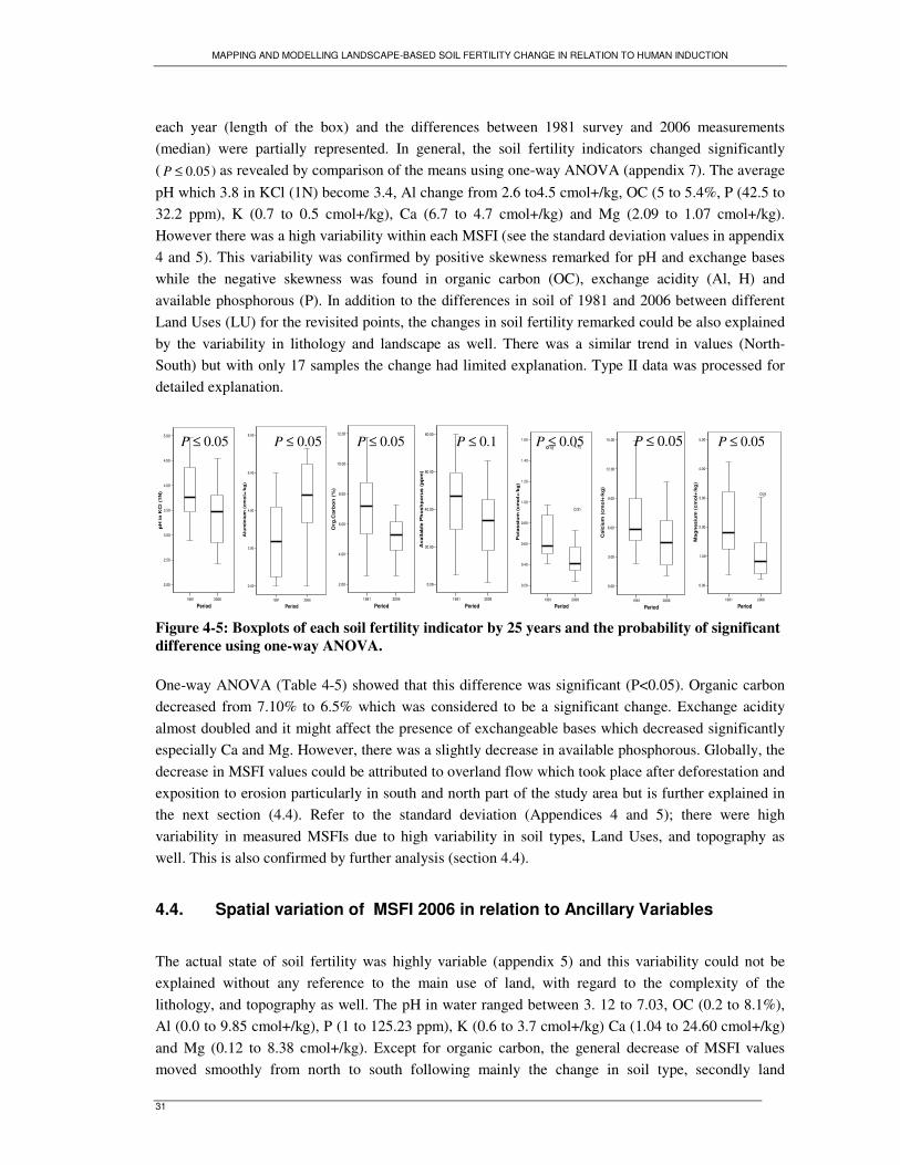
MAPPING AND MODELLING LANDSCAPE-BASED SOIL FERTILITY CHANGE IN RELATION TO HUMAN INDUCTION
31
each year (length of the box) and the differences between 1981 survey and 2006 measurements (median) were partially represented. In general, the soil fertility indicators changed significantly ( 05.0≤P ) as revealed by comparison of the means using one-way ANOVA (appendix 7). The average pH which 3.8 in KCl (1N) become 3.4, Al change from 2.6 to4.5 cmol+/kg, OC (5 to 5.4%, P (42.5 to 32.2 ppm), K (0.7 to 0.5 cmol+/kg), Ca (6.7 to 4.7 cmol+/kg) and Mg (2.09 to 1.07 cmol+/kg). However there was a high variability within each MSFI (see the standard deviation values in appendix 4 and 5). This variability was confirmed by positive skewness remarked for pH and exchange bases while the negative skewness was found in organic carbon (OC), exchange acidity (Al, H) and available phosphorous (P). In addition to the differences in soil of 1981 and 2006 between different Land Uses (LU) for the revisited points, the changes in soil fertility remarked could be also explained by the variability in lithology and landscape as well. There was a similar trend in values (North-South) but with only 17 samples the change had limited explanation. Type II data was processed for detailed explanation.
1981 2006
Period
2.00
2.50
3.00
3.50
4.00
4.50
5.00
pH
in
KC
l (1
N)
1981 2006
Period
0.00
2.00
4.00
6.00
8.00
Alu
min
ium
(cm
ol+
/kg
)
1981 2006
Period
2.00
4.00
6.00
8.00
10.00
12.00
Org
.Carb
on
(%
)
1981 2006
Period
0.00
20.00
40.00
60.00
80.00
Av
ail
ab
le P
ho
sh
po
rus
(p
pm
)
1981 2006
Period
0.20
0.40
0.60
0.80
1.00
1.20
1.40
1.60
Po
tas
siu
m (
cm
ol+
/kg
)
18
31
15
1981 2006
Period
0.00
3.00
6.00
9.00
12.00
15.00
Ca
lciu
m (
cm
ol+
/kg
)
1981 2006
Period
0.00
1.00
2.00
3.00
4.00
5.00
Ma
gn
esiu
m (
cm
ol+
/kg
)
21
Figure 4-5: Boxplots of each soil fertility indicator by 25 years and the probability of significant difference using one-way ANOVA. One-way ANOVA (Table 4-5) showed that this difference was significant (P<0.05). Organic carbon decreased from 7.10% to 6.5% which was considered to be a significant change. Exchange acidity almost doubled and it might affect the presence of exchangeable bases which decreased significantly especially Ca and Mg. However, there was a slightly decrease in available phosphorous. Globally, the decrease in MSFI values could be attributed to overland flow which took place after deforestation and exposition to erosion particularly in south and north part of the study area but is further explained in the next section (4.4). Refer to the standard deviation (Appendices 4 and 5); there were high variability in measured MSFIs due to high variability in soil types, Land Uses, and topography as well. This is also confirmed by further analysis (section 4.4).
4.4. Spatial variation of MSFI 2006 in relation to Ancillary Variables
The actual state of soil fertility was highly variable (appendix 5) and this variability could not be explained without any reference to the main use of land, with regard to the complexity of the lithology, and topography as well. The pH in water ranged between 3. 12 to 7.03, OC (0.2 to 8.1%), Al (0.0 to 9.85 cmol+/kg), P (1 to 125.23 ppm), K (0.6 to 3.7 cmol+/kg) Ca (1.04 to 24.60 cmol+/kg) and Mg (0.12 to 8.38 cmol+/kg). Except for organic carbon, the general decrease of MSFI values moved smoothly from north to south following mainly the change in soil type, secondly land
05.0≤P 05.0≤P 05.0≤P 1.0≤P 05.0≤P 05.0≤P 05.0≤P
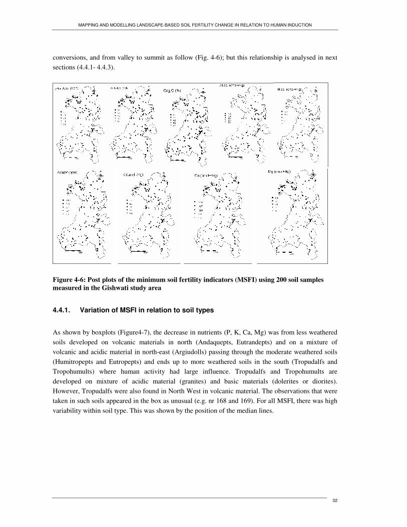
MAPPING AND MODELLING LANDSCAPE-BASED SOIL FERTILITY CHANGE IN RELATION TO HUMAN INDUCTION
32
conversions, and from valley to summit as follow (Fig. 4-6); but this relationship is analysed in next sections (4.4.1- 4.4.3).
Figure 4-6: Post plots of the minimum soil fertility indicators (MSFI) using 200 soil samples measured in the Gishwati study area
4.4.1. Variation of MSFI in relation to soil types
As shown by boxplots (Figure4-7), the decrease in nutrients (P, K, Ca, Mg) was from less weathered soils developed on volcanic materials in north (Andaquepts, Eutrandepts) and on a mixture of volcanic and acidic material in north-east (Argiudolls) passing through the moderate weathered soils (Humitropepts and Eutropepts) and ends up to more weathered soils in the south (Tropudalfs and Tropohumults) where human activity had large influence. Tropudalfs and Tropohumults are developed on mixture of acidic material (granites) and basic materials (dolerites or diorites). However, Tropudalfs were also found in North West in volcanic material. The observations that were taken in such soils appeared in the box as unusual (e.g. nr 168 and 169). For all MSFI, there was high variability within soil type. This was shown by the position of the median lines.
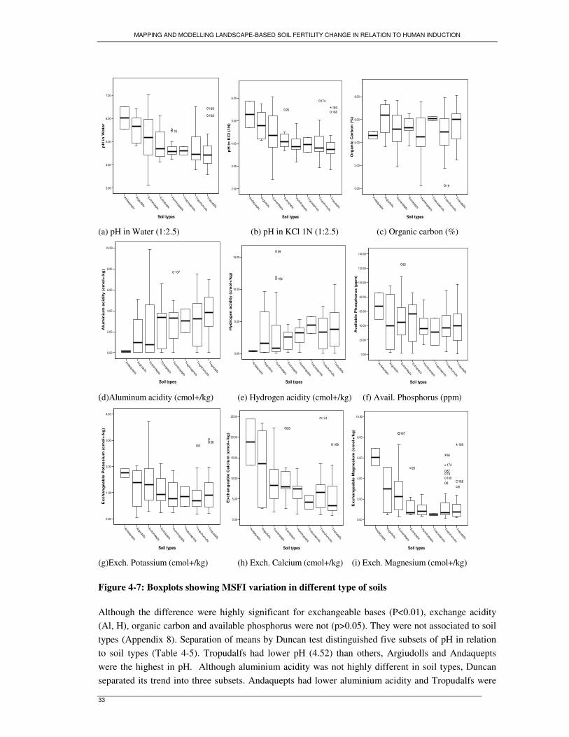
MAPPING AND MODELLING LANDSCAPE-BASED SOIL FERTILITY CHANGE IN RELATION TO HUMAN INDUCTION
33
Andaquepts
Argiudolls
Eutrandepts
Eutropepts
Humitropepts
Troposaprists
Tropohumults
Tropudalfs
Soil types
3.00
4.00
5.00
6.00
7.00
pH
in
Wa
ter
18
168
169
Andaquepts
Argiudolls
Eutrandepts
Eutropepts
Humitropepts
Troposaprists
Tropohumults
Tropudalfs
Soil types
2.00
3.00
4.00
5.00
6.00
pH
in
KC
l (1
N)
26
174
168169
Andaquepts
Argiudolls
Eutrandepts
Eutropepts
Humitropepts
Troposaprists
Tropohumults
Tropudalfs
Soil types
0.00
2.00
4.00
6.00
8.00
Org
an
ic C
arb
on
(%
)
19
(a) pH in Water (1:2.5) (b) pH in KCl 1N (1:2.5) (c) Organic carbon (%)
Andaquepts
Argiudolls
Eutrandepts
Eutropepts
Humitropepts
Troposaprists
Tropohumults
Tropudalfs
Soil types
0.00
2.00
4.00
6.00
8.00
10.00
Alu
min
ium
ac
idit
y (
cm
ol+
/kg
)
137
Andaquepts
Argiudolls
Eutrandepts
Eutropepts
Humitropepts
Troposaprists
Tropohumults
Tropudalfs
Soil types
0.00
5.00
10.00
15.00
Hy
dro
gen
acid
ity (
cm
ol+
/kg
)
194
59
Andaquepts
Argiudolls
Eutrandepts
Eutropepts
Humitropepts
Troposaprists
Tropohumults
Tropudalfs
Soil types
0.00
20.00
40.00
60.00
80.00
100.00
120.00
140.00
Av
ail
ab
le P
ho
sp
ho
rus
(p
pm
)
82
(d)Aluminum acidity (cmol+/kg) (e) Hydrogen acidity (cmol+/kg) (f) Avail. Phosphorus (ppm)
Andaquepts
Argiudolls
Eutrandepts
Eutropepts
Humitropepts
Troposaprists
Tropohumults
Tropudalfs
Soil types
0.00
1.00
2.00
3.00
4.00
Ex
ch
an
gea
ble
Po
tas
siu
m (
cm
ol+
/kg
)
836
Andaquepts
Argiudolls
Eutrandepts
Eutropepts
Humitropepts
Troposaprists
Tropohumults
Tropudalfs
Soil types
0.00
5.00
10.00
15.00
20.00
25.00
Ex
ch
an
gea
ble
Calc
ium
(cm
ol+
/kg
)
26
174
169
Andaquepts
Argiudolls
Eutrandepts
Eutropepts
Humitropepts
Troposaprists
Tropohumults
Tropudalfs
Soil types
0.00
2.00
4.00
6.00
8.00
10.00
Ex
ch
an
ge
ab
le M
ag
ne
siu
m (
cm
ol+
/kg
)
167
26
81007987
6168
174
86
169
(g)Exch. Potassium (cmol+/kg) (h) Exch. Calcium (cmol+/kg) (i) Exch. Magnesium (cmol+/kg)
Figure 4-7: Boxplots showing MSFI variation in different type of soils Although the difference were highly significant for exchangeable bases (P<0.01), exchange acidity (Al, H), organic carbon and available phosphorus were not (p>0.05). They were not associated to soil types (Appendix 8). Separation of means by Duncan test distinguished five subsets of pH in relation to soil types (Table 4-5). Tropudalfs had lower pH (4.52) than others, Argiudolls and Andaquepts were the highest in pH. Although aluminium acidity was not highly different in soil types, Duncan separated its trend into three subsets. Andaquepts had lower aluminium acidity and Tropudalfs were
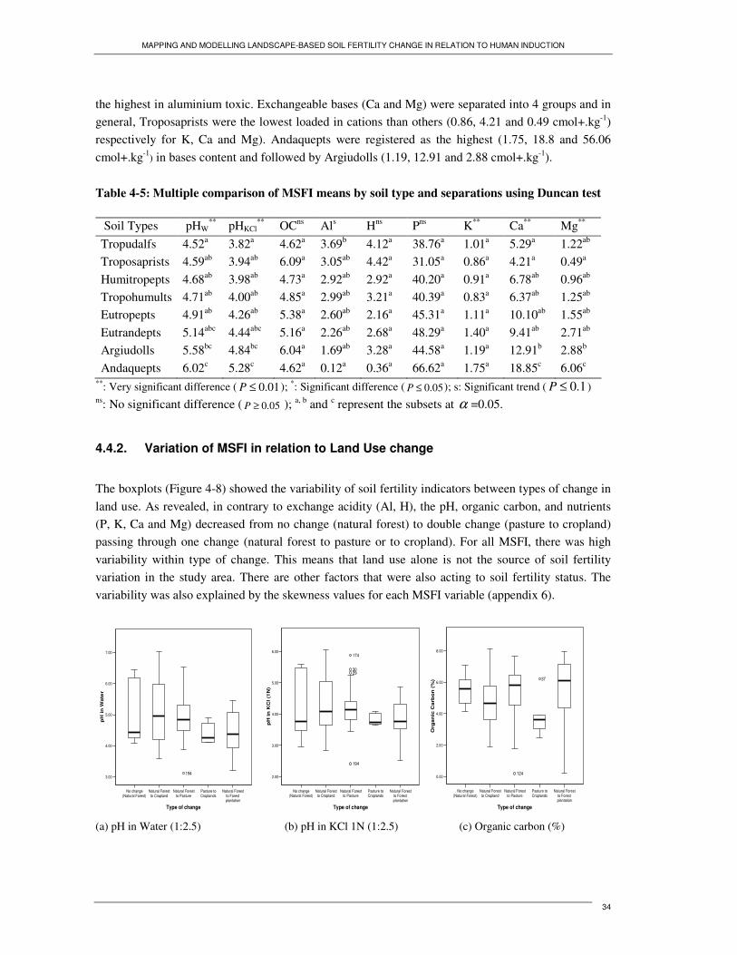
MAPPING AND MODELLING LANDSCAPE-BASED SOIL FERTILITY CHANGE IN RELATION TO HUMAN INDUCTION
34
the highest in aluminium toxic. Exchangeable bases (Ca and Mg) were separated into 4 groups and in general, Troposaprists were the lowest loaded in cations than others (0.86, 4.21 and 0.49 cmol+.kg-1) respectively for K, Ca and Mg). Andaquepts were registered as the highest (1.75, 18.8 and 56.06
cmol+.kg-1) in bases content and followed by Argiudolls (1.19, 12.91 and 2.88 cmol+.kg-1). Table 4-5: Multiple comparison of MSFI means by soil type and separations using Duncan test Soil Types pHW
** pHKCl** OCns Als Hns Pns K** Ca** Mg**
Tropudalfs 4.52a 3.82a 4.62a 3.69b 4.12a 38.76a 1.01a 5.29a 1.22ab Troposaprists 4.59ab 3.94ab 6.09a 3.05ab 4.42a 31.05a 0.86a 4.21a 0.49a Humitropepts 4.68ab 3.98ab 4.73a 2.92ab 2.92a 40.20a 0.91a 6.78ab 0.96ab Tropohumults 4.71ab 4.00ab 4.85a 2.99ab 3.21a 40.39a 0.83a 6.37ab 1.25ab Eutropepts 4.91ab 4.26ab 5.38a 2.60ab 2.16a 45.31a 1.11a 10.10ab 1.55ab Eutrandepts 5.14abc 4.44abc 5.16a 2.26ab 2.68a 48.29a 1.40a 9.41ab 2.71ab Argiudolls 5.58bc 4.84bc 6.04a 1.69ab 3.28a 44.58a 1.19a 12.91b 2.88b Andaquepts 6.02c 5.28c 4.62a 0.12a 0.36a 66.62a 1.75a 18.85c 6.06c
**: Very significant difference ( 01.0≤P ); *: Significant difference ( 05.0≤P ); s: Significant trend ( 1.0≤P ) ns: No significant difference ( 05.0≥P ); a, b and c represent the subsets at α =0.05.
4.4.2. Variation of MSFI in relation to Land Use change
The boxplots (Figure 4-8) showed the variability of soil fertility indicators between types of change in land use. As revealed, in contrary to exchange acidity (Al, H), the pH, organic carbon, and nutrients (P, K, Ca and Mg) decreased from no change (natural forest) to double change (pasture to cropland) passing through one change (natural forest to pasture or to cropland). For all MSFI, there was high variability within type of change. This means that land use alone is not the source of soil fertility variation in the study area. There are other factors that were also acting to soil fertility status. The variability was also explained by the skewness values for each MSFI variable (appendix 6).
No change (Natural Forest)
Natural Forest to Cropland
Natural Forest to Pasture
Pasture to Croplands
Natural Forest to Forest plantation
Type of change
3.00
4.00
5.00
6.00
7.00
pH
in
Wate
r
194
No change (Natural Forest)
Natural Forest to Cropland
Natural Forest to Pasture
Pasture to Croplands
Natural Forest to Forest plantation
Type of change
2.00
3.00
4.00
5.00
6.00
pH
in
KC
l (1
N)
194
2930
174
No change (Natural Forest)
Natural Forest to Cropland
Natural Forest to Pasture
Pasture to Croplands
Natural Forest to Forest plantation
Type of change
0.00
2.00
4.00
6.00
8.00
Org
an
ic C
arb
on
(%
)
124
37
(a) pH in Water (1:2.5) (b) pH in KCl 1N (1:2.5) (c) Organic carbon (%)
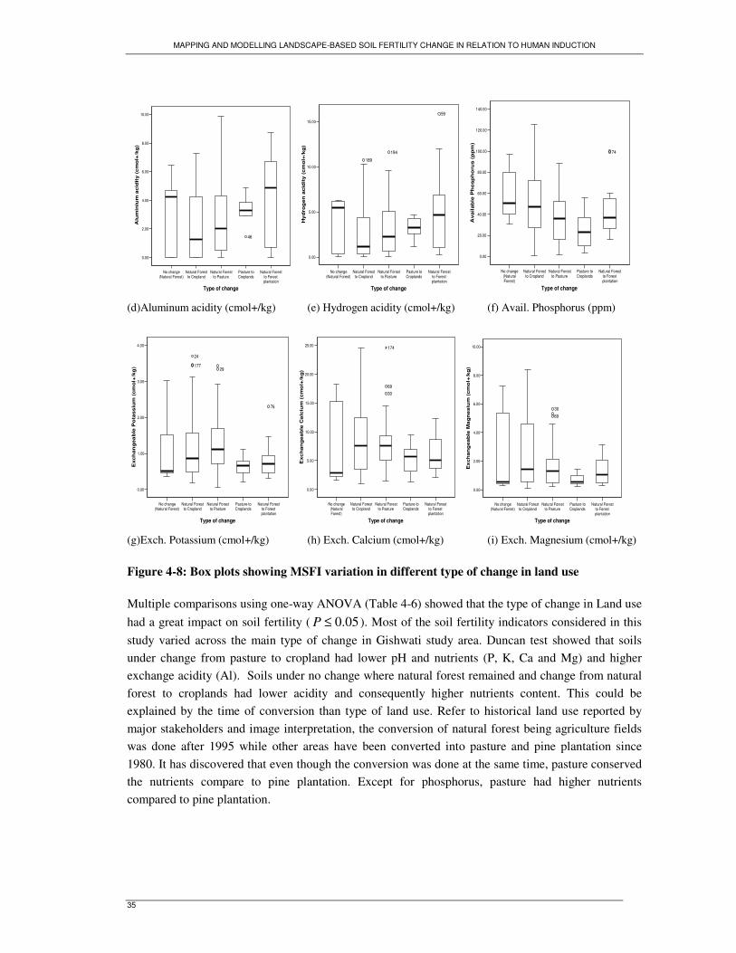
MAPPING AND MODELLING LANDSCAPE-BASED SOIL FERTILITY CHANGE IN RELATION TO HUMAN INDUCTION
35
No change (Natural Forest)
Natural Forest to Cropland
Natural Forest to Pasture
Pasture to Croplands
Natural Forest to Forest plantation
Type of change
0.00
2.00
4.00
6.00
8.00
10.00
Alu
min
ium
acid
ity (
cm
ol+
/kg
)
46
No change (Natural Forest)
Natural Forest to Cropland
Natural Forest to Pasture
Pasture to Croplands
Natural Forest to Forest plantation
Type of change
0.00
5.00
10.00
15.00
Hy
dro
gen
acid
ity (
cm
ol+
/kg
)
189
194
59
No change (Natural Forest)
Natural Forest to Cropland
Natural Forest to Pasture
Pasture to Croplands
Natural Forest to Forest plantation
Type of change
0.00
20.00
40.00
60.00
80.00
100.00
120.00
140.00
Ava
ilab
le P
ho
sp
ho
rus
(p
pm
)
74
(d)Aluminum acidity (cmol+/kg) (e) Hydrogen acidity (cmol+/kg) (f) Avail. Phosphorus (ppm)
No change (Natural Forest)
Natural Forest to Cropland
Natural Forest to Pasture
Pasture to Croplands
Natural Forest to Forest plantation
Type of change
0.00
1.00
2.00
3.00
4.00
Exch
an
gea
ble
Po
tass
ium
(cm
ol+
/kg
) 177
24
29
76
No change (Natural Forest)
Natural Forest to Cropland
Natural Forest to Pasture
Pasture to Croplands
Natural Forest to Forest plantation
Type of change
0.00
5.00
10.00
15.00
20.00
25.00
Exc
han
gea
ble
Ca
lciu
m (
cm
ol+
/kg
)
3069
174
No change (Natural Forest)
Natural Forest to Cropland
Natural Forest to Pasture
Pasture to Croplands
Natural Forest to Forest plantation
Type of change
0.00
2.00
4.00
6.00
8.00
10.00
Ex
ch
an
geab
le M
ag
nesiu
m (
cm
ol+
/kg
)
69
30
(g)Exch. Potassium (cmol+/kg) (h) Exch. Calcium (cmol+/kg) (i) Exch. Magnesium (cmol+/kg)
Figure 4-8: Box plots showing MSFI variation in different type of change in land use Multiple comparisons using one-way ANOVA (Table 4-6) showed that the type of change in Land use had a great impact on soil fertility ( 05.0≤P ). Most of the soil fertility indicators considered in this study varied across the main type of change in Gishwati study area. Duncan test showed that soils under change from pasture to cropland had lower pH and nutrients (P, K, Ca and Mg) and higher exchange acidity (Al). Soils under no change where natural forest remained and change from natural forest to croplands had lower acidity and consequently higher nutrients content. This could be explained by the time of conversion than type of land use. Refer to historical land use reported by major stakeholders and image interpretation, the conversion of natural forest being agriculture fields was done after 1995 while other areas have been converted into pasture and pine plantation since 1980. It has discovered that even though the conversion was done at the same time, pasture conserved the nutrients compare to pine plantation. Except for phosphorus, pasture had higher nutrients compared to pine plantation.
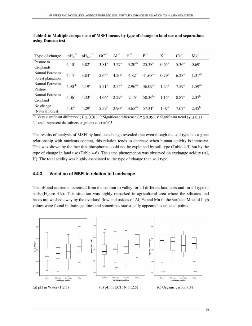
MAPPING AND MODELLING LANDSCAPE-BASED SOIL FERTILITY CHANGE IN RELATION TO HUMAN INDUCTION
36
Table 4-6: Multiple comparison of MSFI means by type of change in land use and separations using Duncan test Type of change pHw
** pHKCl** OC** Al** H** P** K* Cas Mg*
Pasture to Croplands
4.40a 3.82a 3.81a 3.27a 3.20ab 25.38a 0.65a 5.36a 0.69a
Natural Forest to Forest plantation
4.44a 3.84a 5.64b 4.20a 4.82b 41.68abc 0.79a 6.28a 1.31ab
Natural Forest to Pasture
4.90ab 4.19a 5.51b 2.54a 2.96ab 36.09ab 1.24a 7.59a 1.59ab
Natural Forest to Cropland
5.06b 4.33a 4.66ab 2.29a 2.45a 50.36bc 1.15a 8.87a 2.37b
No change (Natural Forest)
5.07b 4.29a 5.59b 2.90a 3.65ab 57.31c 1.07a 7.67a 2.45b
**: Very significant difference ( 01.0≤P ); *: Significant difference ( 05.0≤P ); s: Significant trend ( 1.0≤P ) a, b and c represent the subsets at groups at α =0.05
The results of analysis of MSFI by land use change revealed that even though the soil type has a great relationship with nutrients content, this relation tends to decrease when human activity is intensive. This was shown by the fact that phosphorus could not be explained by soil type (Table 4-5) but by the type of change in land use (Table 4-6). The same phenomenon was observed on exchange acidity (Al, H). The total acidity was highly associated to the type of change than soil type.
4.4.3. Variation of MSFI in relation to Landscape
The pH and nutrients increased from the summit to valley for all different land uses and for all type of soils (Figure 4-9). This situation was highly remarked in agricultural area where the silicates and bases are washed away by the overland flow and oxides of Al, Fe and Mn in the surface. Most of high values were found in drainage lines and sometimes statistically appeared as unusual points.
Summit Middle slope Lower slope Valley
Landscape position
3.00
4.00
5.00
6.00
7.00
pH
in
Wa
ter
Summit Middle slope Lower slope Valley
Landscape position
2.00
3.00
4.00
5.00
6.00
pH
in
KC
l (1
N)
81
194
Summit Middle slope Lower slope Valley
Landscape position
0.00
2.00
4.00
6.00
8.00
Org
an
ic C
arb
on
(%
)
124 19
(a) pH in Water (1:2.5) (b) pH in KCl 1N (1:2.5) (c) Organic carbon (%)
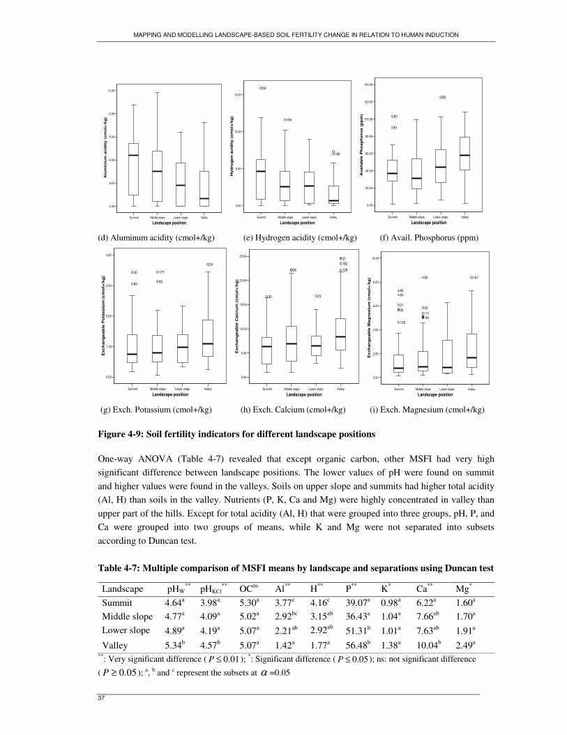
MAPPING AND MODELLING LANDSCAPE-BASED SOIL FERTILITY CHANGE IN RELATION TO HUMAN INDUCTION
37
Summit Middle slope Lower slope Valley
Landscape position
0.00
2.00
4.00
6.00
8.00
10.00
Alu
min
ium
ac
idit
y (
cm
ol+
/kg
)
Summit Middle slope Lower slope Valley
Landscape position
0.00
5.00
10.00
15.00
Hyd
rog
en
ac
idit
y (
cm
ol+
/kg
)
59
194
188
Summit Middle slope Lower slope Valley
Landscape position
0.00
20.00
40.00
60.00
80.00
100.00
120.00
140.00
Ava
ilab
le P
ho
sp
ho
rus
(p
pm
)
81
83
82
(d) Aluminum acidity (cmol+/kg) (e) Hydrogen acidity (cmol+/kg) (f) Avail. Phosphorus (ppm)
Summit Middle slope Lower slope Valley
Landscape position
0.00
1.00
2.00
3.00
4.00
Ex
ch
an
ge
ab
le P
ota
ss
ium
(c
mo
l+/k
g)
83
30
85
177
24
Summit Middle slope Lower slope Valley
Landscape position
0.00
5.00
10.00
15.00
20.00
25.00
Ex
ch
an
ge
ab
le C
alc
ium
(c
mo
l+/k
g)
30
26
23
128
18227
Summit Middle slope Lower slope Valley
Landscape position
0.00
2.00
4.00
6.00
8.00
10.00
Ex
ch
an
gea
ble
Ma
gn
es
ium
(c
mo
l+/k
g)
129
3021
18117122
167
8483
85
(g) Exch. Potassium (cmol+/kg) (h) Exch. Calcium (cmol+/kg) (i) Exch. Magnesium (cmol+/kg)
Figure 4-9: Soil fertility indicators for different landscape positions One-way ANOVA (Table 4-7) revealed that except organic carbon, other MSFI had very high significant difference between landscape positions. The lower values of pH were found on summit and higher values were found in the valleys. Soils on upper slope and summits had higher total acidity (Al, H) than soils in the valley. Nutrients (P, K, Ca and Mg) were highly concentrated in valley than upper part of the hills. Except for total acidity (Al, H) that were grouped into three groups, pH, P, and Ca were grouped into two groups of means, while K and Mg were not separated into subsets according to Duncan test. Table 4-7: Multiple comparison of MSFI means by landscape and separations using Duncan test Landscape pHW
** pHKCl** OCns Al** H** P** K* Ca** Mg*
Summit 4.64a 3.98a 5.30a 3.77c 4.16c 39.07a 0.98a 6.22a 1.60a Middle slope 4.77a 4.09a 5.02a 2.92bc 3.15ab 36.43a 1.04a 7.66ab 1.70a Lower slope 4.89a 4.19a 5.07a 2.21ab 2.92ab 51.31b 1.01a 7.63ab 1.91a Valley 5.34b 4.57b 5.07a 1.42a 1.77a 56.48b 1.38a 10.04b 2.49a
**: Very significant difference ( 01.0≤P ); *: Significant difference ( 05.0≤P ); ns: not significant difference
( 05.0≥P ); a, b and c represent the subsets at α =0.05
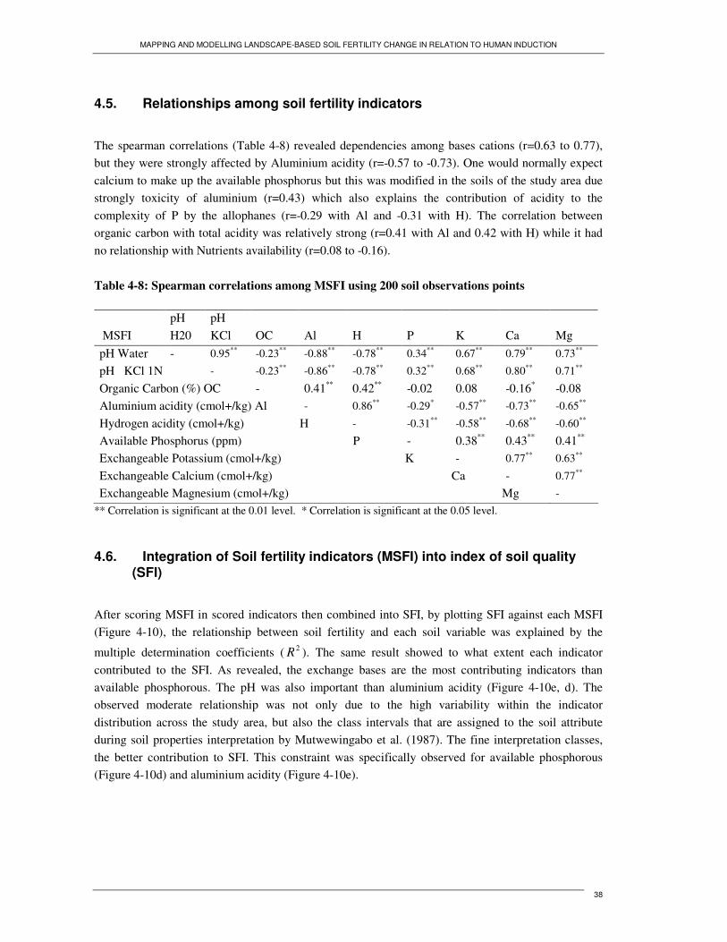
MAPPING AND MODELLING LANDSCAPE-BASED SOIL FERTILITY CHANGE IN RELATION TO HUMAN INDUCTION
38
4.5. Relationships among soil fertility indicators
The spearman correlations (Table 4-8) revealed dependencies among bases cations (r=0.63 to 0.77), but they were strongly affected by Aluminium acidity (r=-0.57 to -0.73). One would normally expect calcium to make up the available phosphorus but this was modified in the soils of the study area due strongly toxicity of aluminium (r=0.43) which also explains the contribution of acidity to the complexity of P by the allophanes (r=-0.29 with Al and -0.31 with H). The correlation between organic carbon with total acidity was relatively strong (r=0.41 with Al and 0.42 with H) while it had no relationship with Nutrients availability (r=0.08 to -0.16). Table 4-8: Spearman correlations among MSFI using 200 soil observations points
MSFI pH H20
pH KCl OC Al H P K Ca Mg
pH Water - 0.95** -0.23** -0.88** -0.78** 0.34** 0.67** 0.79** 0.73**
pH KCl 1N - -0.23** -0.86** -0.78** 0.32** 0.68** 0.80** 0.71**
Organic Carbon (%) OC - 0.41** 0.42** -0.02 0.08 -0.16* -0.08 Aluminium acidity (cmol+/kg) Al - 0.86** -0.29* -0.57** -0.73** -0.65**
Hydrogen acidity (cmol+/kg) H - -0.31** -0.58** -0.68** -0.60**
Available Phosphorus (ppm) P - 0.38** 0.43** 0.41** Exchangeable Potassium (cmol+/kg) K - 0.77** 0.63**
Exchangeable Calcium (cmol+/kg) Ca - 0.77**
Exchangeable Magnesium (cmol+/kg) Mg -
** Correlation is significant at the 0.01 level. * Correlation is significant at the 0.05 level.
4.6. Integration of Soil fertility indicators (MSFI) into index of soil quality (SFI)
After scoring MSFI in scored indicators then combined into SFI, by plotting SFI against each MSFI (Figure 4-10), the relationship between soil fertility and each soil variable was explained by the
multiple determination coefficients ( 2R ). The same result showed to what extent each indicator contributed to the SFI. As revealed, the exchange bases are the most contributing indicators than available phosphorous. The pH was also important than aluminium acidity (Figure 4-10e, d). The observed moderate relationship was not only due to the high variability within the indicator distribution across the study area, but also the class intervals that are assigned to the soil attribute during soil properties interpretation by Mutwewingabo et al. (1987). The fine interpretation classes, the better contribution to SFI. This constraint was specifically observed for available phosphorous (Figure 4-10d) and aluminium acidity (Figure 4-10e).
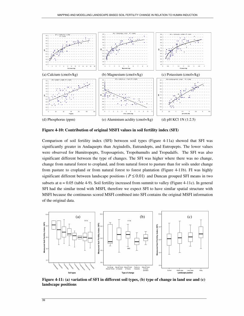
MAPPING AND MODELLING LANDSCAPE-BASED SOIL FERTILITY CHANGE IN RELATION TO HUMAN INDUCTION
39
SFI = 1.5408Ln(Ca) + 3.7839R2 = 0.8194
4.0
4.5
5.0
5.5
6.0
6.5
7.0
7.5
8.0
8.5
9.0
9.5
1 3 5 7 9 11 13 15 17 19 21 23 25
Ca (cmol+/kg)
SF
I
SFI= 1.0324Ln(Mg) + 6.313 R2 = 0.8093
4.0
4.5
5.0
5.5
6.0
6.5
7.0
7.5
8.0
8.5
9.0
9.5
0 1 2 3 4 5 6 7 8 9
Mg (cmol+/kg)
SF
I
SFI = 1.3414Ln(K) + 6.7698 R2 = 0.641
4.0
4.5
5.0
5.5
6.0
6.5
7.0
7.5
8.0
8.5
9.0
9.5
0 0.5 1 1.5 2 2.5 3 3.5 4
K (cmol+/kg)
SFI
(a) Calcium (cmol+/kg) (b) Magnesium (cmol+/kg) (c) Potassium (cmol+/kg)
SFI = 0.0296 P + 5.6089 R2 = 0.4907
4.0
4.5
5.0
5.5
6.0
6.5
7.0
7.5
8.0
8.5
9.0
9.5
0 20 40 60 80 100 120
P (ppm)
SF
I
SFI = -0.328 AL ac. + 7.6413 R2 = 0.6259
4.0
4.5
5.0
5.5
6.0
6.5
7.0
7.5
8.0
8.5
9.0
9.5
0 1 2 3 4 5 6 7 8 9 10 11
Al ac. (cmol+/kg)
SFI
SFI= 6.2203Ln(pH KCl) - 2.3443 R2 = 0.7822
4.5
5.0
5.5
6.0
6.5
7.0
7.5
8.0
8.5
9.0
9.5
3 3.5 4 4.5 5 5.5 6 6.5
pH in KCl (1N)
SFI
(d) Phosphorus (ppm) (e) Aluminium acidity (cmol+/kg) (d) pH KCl 1N (1:2.5)
Figure 4-10: Contribution of original MSFI values in soil fertility index (SFI) Comparison of soil fertility index (SFI) between soil types (Figure 4-11a) showed that SFI was significantly greater in Andaquepts than Argiudolls, Eutrandepts, and Eutropepts. The lower values were observed for Humitropepts, Troposaprists, Tropohumults and Tropudalfs. The SFI was also significant different between the type of changes. The SFI was higher where there was no change, change from natural forest to cropland, and from natural forest to pasture than for soils under change from pasture to cropland or from natural forest to forest plantation (Figure 4-11b). FI was highly significant different between landscape positions ( )01.0≤P and Duncan grouped SFI means in two
subsets at � = 0.05 (table 4-9). Soil fertility increased from summit to valley (Figure 4-11c). In general SFI had the similar trend with MSFI, therefore we expect SFI to have similar spatial structure with MSFI because the continuous scored MSFI combined into SFI contains the original MSFI information of the original data.
Andaquepts
Argiudolls
Eutrandepts
Eutropepts
Humitropepts
Troposaprists
Tropohumults
Tropudalfs
Soil types
2.0
4.0
6.0
8.0
10.0
Me
asu
red
So
il F
ert
ilit
y In
dex (
SF
I)
174
No change (Natural Forest)
Natural Forest to Cropland
Natural Forest to Pasture
Pasture to Croplands
Natural Forest to Forest plantation
Type of change
2.0
4.0
6.0
8.0
10.0
Mea
sure
d S
oil
Fe
rtili
ty In
dex
(S
FI)
45
174
Summit Middle slope Lower slope Valley
Landscape position
2.0
4.0
6.0
8.0
10.0
Me
as
ure
d S
oil F
ert
ilit
y I
nd
ex (
SF
I)
Figure 4-11: (a) variation of SFI in different soil types, (b) type of change in land use and (c) landscape positions
(a) (b) (c)
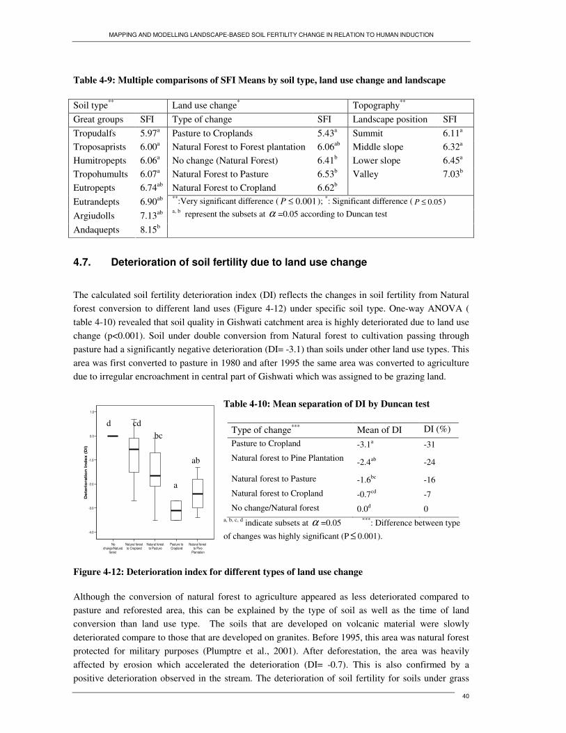
MAPPING AND MODELLING LANDSCAPE-BASED SOIL FERTILITY CHANGE IN RELATION TO HUMAN INDUCTION
40
Table 4-9: Multiple comparisons of SFI Means by soil type, land use change and landscape Soil type** Land use change* Topography** Great groups SFI Type of change SFI Landscape position SFI Tropudalfs 5.97a Pasture to Croplands 5.43a Summit 6.11a Troposaprists 6.00a Natural Forest to Forest plantation 6.06ab Middle slope 6.32a Humitropepts 6.06a No change (Natural Forest) 6.41b Lower slope 6.45a Tropohumults 6.07a Natural Forest to Pasture 6.53b Valley 7.03b Eutropepts 6.74ab Natural Forest to Cropland 6.62b Eutrandepts 6.90ab Argiudolls 7.13ab Andaquepts 8.15b
**:Very significant difference ( 001.0≤P ); *: Significant difference ( 05.0≤P ) a, b represent the subsets at α =0.05 according to Duncan test
4.7. Deterioration of soil fertility due to land use change
The calculated soil fertility deterioration index (DI) reflects the changes in soil fertility from Natural forest conversion to different land uses (Figure 4-12) under specific soil type. One-way ANOVA ( table 4-10) revealed that soil quality in Gishwati catchment area is highly deteriorated due to land use change (p<0.001). Soil under double conversion from Natural forest to cultivation passing through pasture had a significantly negative deterioration (DI= -3.1) than soils under other land use types. This area was first converted to pasture in 1980 and after 1995 the same area was converted to agriculture due to irregular encroachment in central part of Gishwati which was assigned to be grazing land.
Table 4-10: Mean separation of DI by Duncan test
Type of change*** Mean of DI DI (%) Pasture to Cropland -3.1a -31
Natural forest to Pine Plantation -2.4ab -24
Natural forest to Pasture -1.6bc -16
Natural forest to Cropland -0.7cd -7
No change/Natural forest 0.0d 0 a, b, c, d indicate subsets at α =0.05 ***: Difference between type
of changes was highly significant (P ≤ 0.001).
Figure 4-12: Deterioration index for different types of land use change Although the conversion of natural forest to agriculture appeared as less deteriorated compared to pasture and reforested area, this can be explained by the type of soil as well as the time of land conversion than land use type. The soils that are developed on volcanic material were slowly deteriorated compare to those that are developed on granites. Before 1995, this area was natural forest protected for military purposes (Plumptre et al., 2001). After deforestation, the area was heavily affected by erosion which accelerated the deterioration (DI= -0.7). This is also confirmed by a positive deterioration observed in the stream. The deterioration of soil fertility for soils under grass
No change/Natural
forest
Natural forest to Cropland
Natural forest to Pasture
Pasture to Cropland
Natural forest to Pine
Plantation
-4.0
-3.0
-2.0
-1.0
0.0
1.0
Dete
rio
rati
on
In
dex (
DI)
d cd bc ab
a
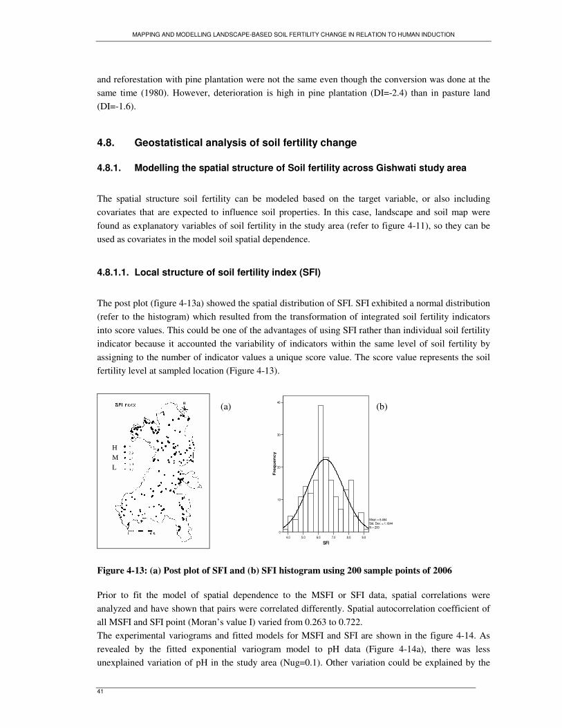
MAPPING AND MODELLING LANDSCAPE-BASED SOIL FERTILITY CHANGE IN RELATION TO HUMAN INDUCTION
41
and reforestation with pine plantation were not the same even though the conversion was done at the same time (1980). However, deterioration is high in pine plantation (DI=-2.4) than in pasture land (DI=-1.6).
4.8. Geostatistical analysis of soil fertility change
4.8.1. Modelling the spatial structure of Soil fertility across Gishwati study area
The spatial structure soil fertility can be modeled based on the target variable, or also including covariates that are expected to influence soil properties. In this case, landscape and soil map were found as explanatory variables of soil fertility in the study area (refer to figure 4-11), so they can be used as covariates in the model soil spatial dependence.
4.8.1.1. Local structure of soil fertility index (SFI)
The post plot (figure 4-13a) showed the spatial distribution of SFI. SFI exhibited a normal distribution (refer to the histogram) which resulted from the transformation of integrated soil fertility indicators into score values. This could be one of the advantages of using SFI rather than individual soil fertility indicator because it accounted the variability of indicators within the same level of soil fertility by assigning to the number of indicator values a unique score value. The score value represents the soil fertility level at sampled location (Figure 4-13).
4.0 5.0 6.0 7.0 8.0 9.0
SFI
0
10
20
30
40
Fre
qu
en
cy
Mean = 6.464Std. Dev. = 1.1844N = 200
Figure 4-13: (a) Post plot of SFI and (b) SFI histogram using 200 sample points of 2006 Prior to fit the model of spatial dependence to the MSFI or SFI data, spatial correlations were analyzed and have shown that pairs were correlated differently. Spatial autocorrelation coefficient of all MSFI and SFI point (Moran’s value I) varied from 0.263 to 0.722. The experimental variograms and fitted models for MSFI and SFI are shown in the figure 4-14. As revealed by the fitted exponential variogram model to pH data (Figure 4-14a), there was less unexplained variation of pH in the study area (Nug=0.1). Other variation could be explained by the
H M L
(a) (b)
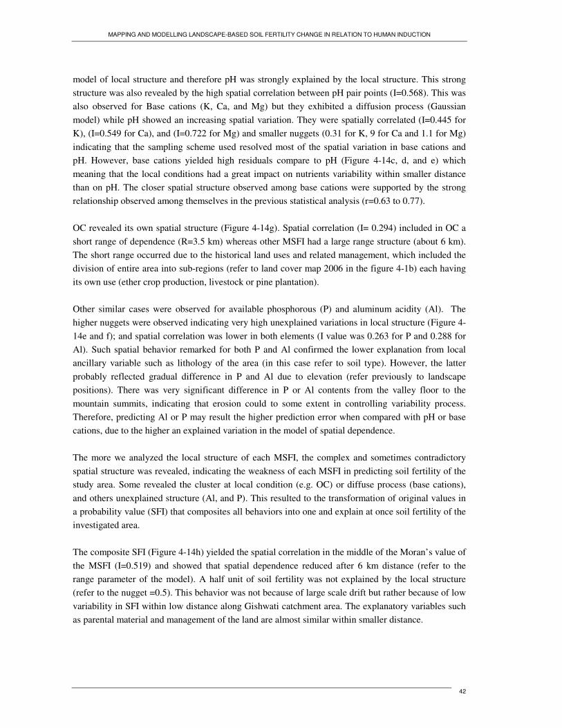
MAPPING AND MODELLING LANDSCAPE-BASED SOIL FERTILITY CHANGE IN RELATION TO HUMAN INDUCTION
42
model of local structure and therefore pH was strongly explained by the local structure. This strong structure was also revealed by the high spatial correlation between pH pair points (I=0.568). This was also observed for Base cations (K, Ca, and Mg) but they exhibited a diffusion process (Gaussian model) while pH showed an increasing spatial variation. They were spatially correlated (I=0.445 for K), (I=0.549 for Ca), and (I=0.722 for Mg) and smaller nuggets (0.31 for K, 9 for Ca and 1.1 for Mg) indicating that the sampling scheme used resolved most of the spatial variation in base cations and pH. However, base cations yielded high residuals compare to pH (Figure 4-14c, d, and e) which meaning that the local conditions had a great impact on nutrients variability within smaller distance than on pH. The closer spatial structure observed among base cations were supported by the strong relationship observed among themselves in the previous statistical analysis (r=0.63 to 0.77). OC revealed its own spatial structure (Figure 4-14g). Spatial correlation (I= 0.294) included in OC a short range of dependence (R=3.5 km) whereas other MSFI had a large range structure (about 6 km). The short range occurred due to the historical land uses and related management, which included the division of entire area into sub-regions (refer to land cover map 2006 in the figure 4-1b) each having its own use (ether crop production, livestock or pine plantation). Other similar cases were observed for available phosphorous (P) and aluminum acidity (Al). The higher nuggets were observed indicating very high unexplained variations in local structure (Figure 4-14e and f); and spatial correlation was lower in both elements (I value was 0.263 for P and 0.288 for Al). Such spatial behavior remarked for both P and Al confirmed the lower explanation from local ancillary variable such as lithology of the area (in this case refer to soil type). However, the latter probably reflected gradual difference in P and Al due to elevation (refer previously to landscape positions). There was very significant difference in P or Al contents from the valley floor to the mountain summits, indicating that erosion could to some extent in controlling variability process. Therefore, predicting Al or P may result the higher prediction error when compared with pH or base cations, due to the higher an explained variation in the model of spatial dependence. The more we analyzed the local structure of each MSFI, the complex and sometimes contradictory spatial structure was revealed, indicating the weakness of each MSFI in predicting soil fertility of the study area. Some revealed the cluster at local condition (e.g. OC) or diffuse process (base cations), and others unexplained structure (Al, and P). This resulted to the transformation of original values in a probability value (SFI) that composites all behaviors into one and explain at once soil fertility of the investigated area. The composite SFI (Figure 4-14h) yielded the spatial correlation in the middle of the Moran’s value of the MSFI (I=0.519) and showed that spatial dependence reduced after 6 km distance (refer to the range parameter of the model). A half unit of soil fertility was not explained by the local structure (refer to the nugget =0.5). This behavior was not because of large scale drift but rather because of low variability in SFI within low distance along Gishwati catchment area. The explanatory variables such as parental material and management of the land are almost similar within smaller distance.
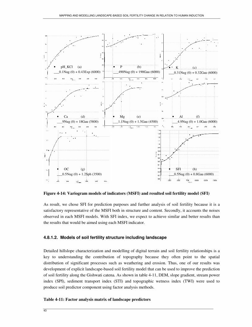
MAPPING AND MODELLING LANDSCAPE-BASED SOIL FERTILITY CHANGE IN RELATION TO HUMAN INDUCTION
43
Figure 4-14: Variogram models of indicators (MSFI) and resulted soil fertility model (SFI) As result, we chose SFI for prediction purposes and further analysis of soil fertility because it is a satisfactory representative of the MSFI both in structure and content. Secondly, it accounts the noises observed in each MSFI models. With SFI index, we expect to achieve similar and better results than the results that would be aimed using each MSFI indicator.
4.8.1.2. Models of soil fertility structure including landscape
Detailed hillslope characterization and modelling of digital terrain and soil fertility relationships is a key to understanding the contribution of topography because they often point to the spatial distribution of significant processes such as weathering and erosion. Thus, one of our results was development of explicit landscape-based soil fertility model that can be used to improve the prediction of soil fertility along the Gishwati catena. As shown in table 4-11, DEM, slope gradient, stream power index (SPI), sediment transport index (STI) and topographic wetness index (TWI) were used to produce soil predictor component using factor analysis methods. Table 4-11: Factor analysis matrix of landscape predictors
• SFI (h) ___0.5Nug (0) + 0.8Gau (6000)
• OC (g) ___0.5Nug (0) + 1.2Sph (3500)
• Ca (d) ___9Nug (0) + 18Gau (5800)
• Mg (e) ___1.1Nug (0) + 1.5Gau (4500)
• Al (f) ___4.9Nug (0) + 1.0Gau (6000)
• pH_KCl (a) ___0.1Nug (0) + 0.43Exp (6000)
• P (b) ___490Nug (0) + 190Gau (6000)
• K (c) ___0.31Nug (0) + 0.32Gau (6000)
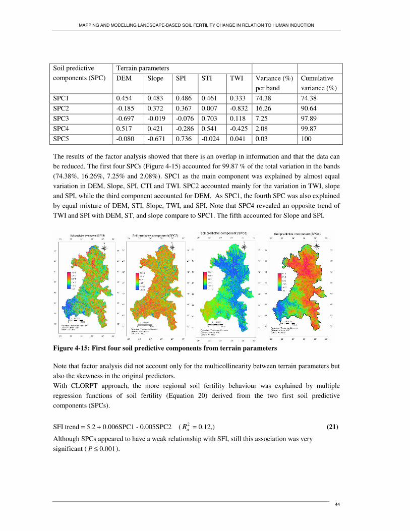
MAPPING AND MODELLING LANDSCAPE-BASED SOIL FERTILITY CHANGE IN RELATION TO HUMAN INDUCTION
44
Terrain parameters Soil predictive
components (SPC) DEM Slope SPI STI TWI Variance (%) per band
Cumulative variance (%)
SPC1 0.454 0.483 0.486 0.461 0.333 74.38 74.38 SPC2 -0.185 0.372 0.367 0.007 -0.832 16.26 90.64 SPC3 -0.697 -0.019 -0.076 0.703 0.118 7.25 97.89 SPC4 0.517 0.421 -0.286 0.541 -0.425 2.08 99.87 SPC5 -0.080 -0.671 0.736 -0.024 0.041 0.03 100 The results of the factor analysis showed that there is an overlap in information and that the data can be reduced. The first four SPCs (Figure 4-15) accounted for 99.87 % of the total variation in the bands (74.38%, 16.26%, 7.25% and 2.08%). SPC1 as the main component was explained by almost equal variation in DEM, Slope, SPI, CTI and TWI. SPC2 accounted mainly for the variation in TWI, slope and SPI, while the third component accounted for DEM. As SPC1, the fourth SPC was also explained by equal mixture of DEM, STI, Slope, TWI, and SPI. Note that SPC4 revealed an opposite trend of TWI and SPI with DEM, ST, and slope compare to SPC1. The fifth accounted for Slope and SPI.
Figure 4-15: First four soil predictive components from terrain parameters Note that factor analysis did not account only for the multicollinearity between terrain parameters but also the skewness in the original predictors. With CLORPT approach, the more regional soil fertility behaviour was explained by multiple regression functions of soil fertility (Equation 20) derived from the two first soil predictive components (SPCs).
SFI trend = 5.2 + 0.006SPC1 - 0.005SPC2 ( 2aR = 0.12,) (21)
Although SPCs appeared to have a weak relationship with SFI, still this association was very significant ( 001.0≤P ).
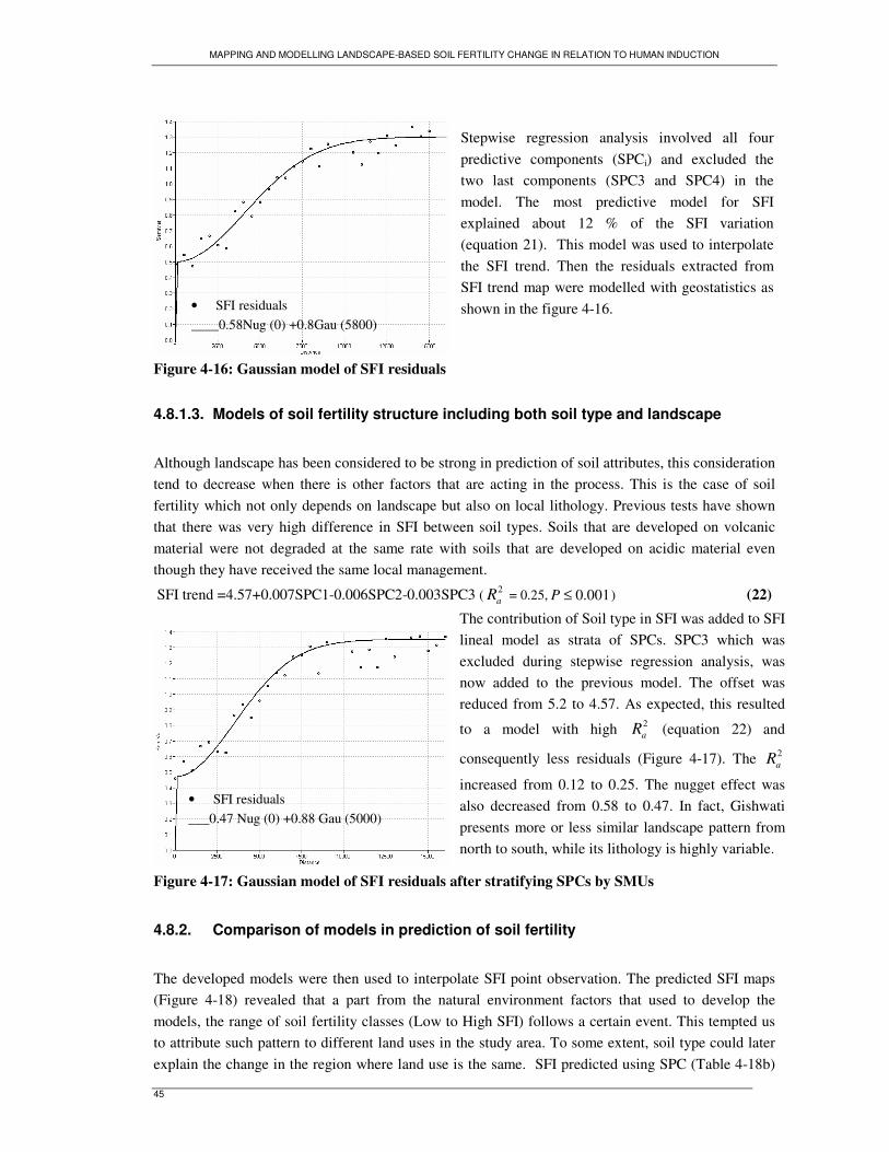
MAPPING AND MODELLING LANDSCAPE-BASED SOIL FERTILITY CHANGE IN RELATION TO HUMAN INDUCTION
45
Figure 4-16: Gaussian model of SFI residuals
4.8.1.3. Models of soil fertility structure including both soil type and landscape
Although landscape has been considered to be strong in prediction of soil attributes, this consideration tend to decrease when there is other factors that are acting in the process. This is the case of soil fertility which not only depends on landscape but also on local lithology. Previous tests have shown that there was very high difference in SFI between soil types. Soils that are developed on volcanic material were not degraded at the same rate with soils that are developed on acidic material even though they have received the same local management.
SFI trend =4.57+0.007SPC1-0.006SPC2-0.003SPC3 ( 2aR = 0.25, 001.0≤P ) (22)
Figure 4-17: Gaussian model of SFI residuals after stratifying SPCs by SMUs
4.8.2. Comparison of models in prediction of soil fertility
The developed models were then used to interpolate SFI point observation. The predicted SFI maps (Figure 4-18) revealed that a part from the natural environment factors that used to develop the models, the range of soil fertility classes (Low to High SFI) follows a certain event. This tempted us to attribute such pattern to different land uses in the study area. To some extent, soil type could later explain the change in the region where land use is the same. SFI predicted using SPC (Table 4-18b)
• SFI residuals ___0.47 Nug (0) +0.88 Gau (5000)
• SFI residuals ____0.58Nug (0) +0.8Gau (5800)
Stepwise regression analysis involved all four predictive components (SPCi) and excluded the two last components (SPC3 and SPC4) in the model. The most predictive model for SFI explained about 12 % of the SFI variation (equation 21). This model was used to interpolate the SFI trend. Then the residuals extracted from SFI trend map were modelled with geostatistics as shown in the figure 4-16.
The contribution of Soil type in SFI was added to SFI lineal model as strata of SPCs. SPC3 which was excluded during stepwise regression analysis, was now added to the previous model. The offset was reduced from 5.2 to 4.57. As expected, this resulted
to a model with high 2aR (equation 22) and
consequently less residuals (Figure 4-17). The 2aR
increased from 0.12 to 0.25. The nugget effect was also decreased from 0.58 to 0.47. In fact, Gishwati presents more or less similar landscape pattern from north to south, while its lithology is highly variable.
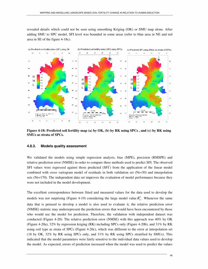
MAPPING AND MODELLING LANDSCAPE-BASED SOIL FERTILITY CHANGE IN RELATION TO HUMAN INDUCTION
46
revealed details which could not be seen using smoothing Kriging (OK) or SMU map alone. After adding SMU to SPC model, SFI level was bounded in some areas (refer to blue area in NE and red area in SE of the figure 4-18c).
Figure 4-18: Predicted soil fertility map (a) by OK, (b) by RK using SPCs , and (c) by RK using SMUs as strata of SPCs.
4.8.3. Models quality assessment
We validated the models using simple regression analysis, bias (MPE), precision (RMSPE) and relative prediction error (NMSE) in order to compare three methods used to predict SFI. The observed SFI values were regressed against those predicted (SFI*) from the application of the linear model combined with cross variogram model of residuals in both validation set (Nr=30) and interpolation sets (Nr=170). The independent data set improves the evaluation of model performance because they were not included in the model development. The excellent correspondence between fitted and measured values for the data used to develop the
models was not surprising (Figure 4-19) considering the large model value 2aR . Whenever the same
data that is perused to develop a model is also used to evaluate it, the relative prediction error (NMSE) statistic may underrepresent the prediction errors that would have been encountered by those who would use the model for prediction. Therefore, the validation with independent dataset was conducted (Figure 4-20). The relative prediction error (NMSE) with this approach was 40% by OK (Figure 4-20a), 32% by regression kriging (RK) including SPCs only (Figure 4-20b), and 31% by RK using soil type as strata of SPCs (Figure 4-20c), which was different to the error at interpolation set (18 by OK, 32% by RK using SPCs only, and 31% by RK using SPCs stratified by SMUs). This indicated that the model parameters were fairly sensitive to the individual data values used to develop the model. As expected, errors of prediction increased when the model was used to predict the values
H M L
H M L
H M L
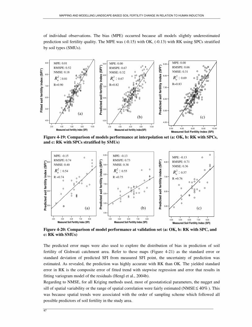
MAPPING AND MODELLING LANDSCAPE-BASED SOIL FERTILITY CHANGE IN RELATION TO HUMAN INDUCTION
47
of individual observations. The bias (MPE) occurred because all models slightly underestimated prediction soil fertility quality. The MPE was (-0.15) with OK, (-0.13) with RK using SPCs stratified by soil types (SMUs).
4.00
5.00
6.00
7.00
8.00
9.00
2.00 4.00 6.00 8.00 10.00
Measured soil fertility index (SFI)
4.00
5.00
6.00
7.00
8.00
9.00
2.00 4.00 6.00 8.00 10.00
Measured soil fertility index(SFI)
4.00
5.00
6.00
7.00
8.00
9.00
2.00 4.00 6.00 8.00 10.00
Measured Soil Fertility Index (SFI) Figure 4-19: Comparison of models performance at interpolation set (a: OK, b: RK with SPCs, and c: RK with SPCs stratified by SMUs)
5.00
6.00
7.00
8.00
4.00 5.00 6.00 7.00 8.00
Measured Soil Fertility Index (SFI)
4.00
5.00
6.00
7.00
8.00
9.00
10.00
4.00 5.00 6.00 7.00 8.00
Measured Soil Fertility Index (SFI)
5.00
6.00
7.00
8.00
4.00 5.00 6.00 7.00 8.00
Measured Soil Fertility Index (SFI) Figure 4-20: Comparison of model performance at validation set (a: OK, b: RK with SPC, and c: RK with SMUs) The predicted error maps were also used to explore the distribution of bias in prediction of soil fertility of Gishwati catchment area. Refer to these maps (Figure 4-21) as the standard error or standard deviation of predicted SFI from measured SFI point, the uncertainty of prediction was estimated. As revealed, the prediction was highly accurate with RK than OK. The yielded standard error in RK is the composite error of fitted trend with stepwise regression and error that results in fitting variogram model of the residuals (Hengl et al., 2004b). Regarding to NMSE, for all Kriging methods used, most of geostatistical parameters, the nugget and sill of spatial variability or the range of spatial correlation were fairly estimated (NMSE %40≤ ). This was because spatial trends were associated with the order of sampling scheme which followed all possible predictors of soil fertility in the study area.
MPE: 0.01 RMSPE: 0.52 NMSE: 0.18
:2aR 0.81
R=0.90
MPE: 0.00 RMSPE: 0.67 NMSE: 0.32
:2aR 0.67
R=0.82
Pre
dict
ed s
oil f
ertil
ity in
dex
(SFI
*)
Fitt
ed s
oil f
ertil
ity in
dex
(SFI
*)
MPE: -0.15 RMSPE: 0.74 NMSE: 0.40
:2aR 0.54
R =0.74
Pre
dict
ed s
oil f
ertil
ity in
dex
(SFI
*)
MPE: -0.13 RMSPE: 0.73 NMSE: 0.38
:2aR 0.55
R =0.75
Pre
dict
ed s
oil f
ertil
ity in
dex
(SFI
*)
Pre
dict
ed s
oil f
ertil
ity in
dex
(SFI
*) MPE: -0.13
RMSPE: 0.71 NMSE: 0.36
:2aR 0.57
R =0.76
Pre
dict
ed s
oil f
ertil
ity in
dex
(SFI
*) MPE: 0.00
RMSPE: 0.66 NMSE: 0.31
:2aR 0.69
R=0.83
(a) (b) (c)
(a) (b) (c)
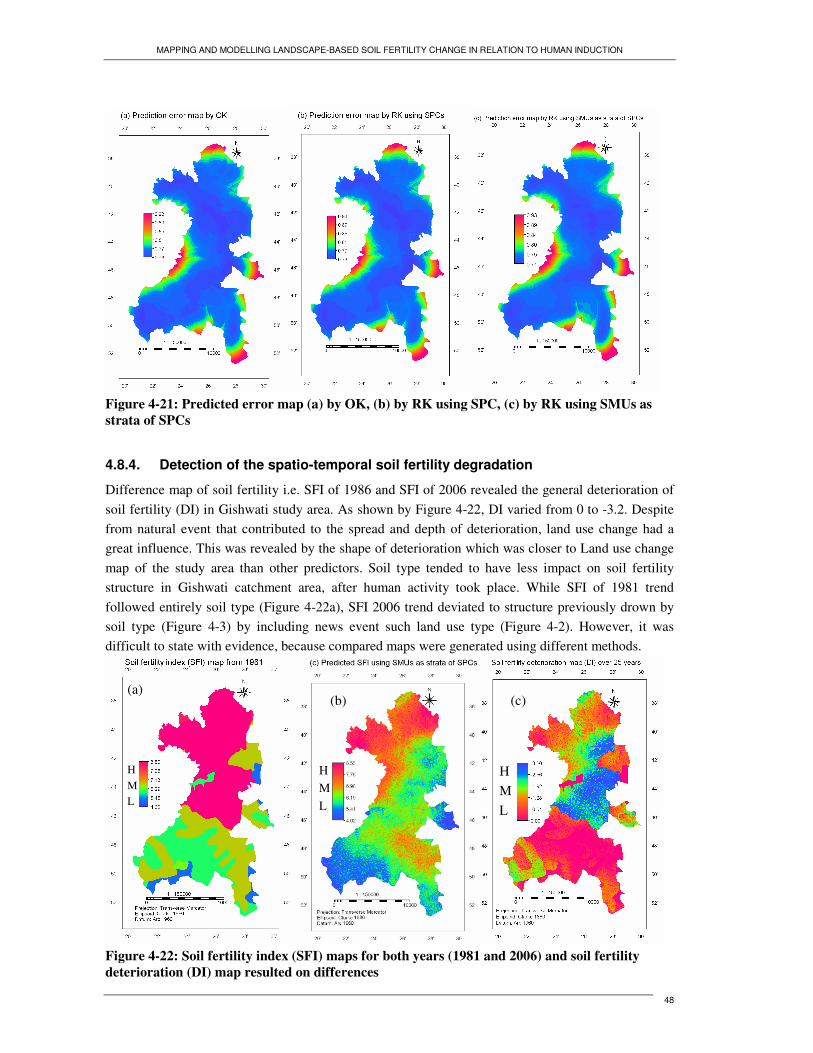
MAPPING AND MODELLING LANDSCAPE-BASED SOIL FERTILITY CHANGE IN RELATION TO HUMAN INDUCTION
48
Figure 4-21: Predicted error map (a) by OK, (b) by RK using SPC, (c) by RK using SMUs as strata of SPCs
4.8.4. Detection of the spatio-temporal soil fertility degradation
Difference map of soil fertility i.e. SFI of 1986 and SFI of 2006 revealed the general deterioration of soil fertility (DI) in Gishwati study area. As shown by Figure 4-22, DI varied from 0 to -3.2. Despite from natural event that contributed to the spread and depth of deterioration, land use change had a great influence. This was revealed by the shape of deterioration which was closer to Land use change map of the study area than other predictors. Soil type tended to have less impact on soil fertility structure in Gishwati catchment area, after human activity took place. While SFI of 1981 trend followed entirely soil type (Figure 4-22a), SFI 2006 trend deviated to structure previously drown by soil type (Figure 4-3) by including news event such land use type (Figure 4-2). However, it was difficult to state with evidence, because compared maps were generated using different methods.
Figure 4-22: Soil fertility index (SFI) maps for both years (1981 and 2006) and soil fertility deterioration (DI) map resulted on differences
H M L
H M L
H M L
(a) (b) (c)
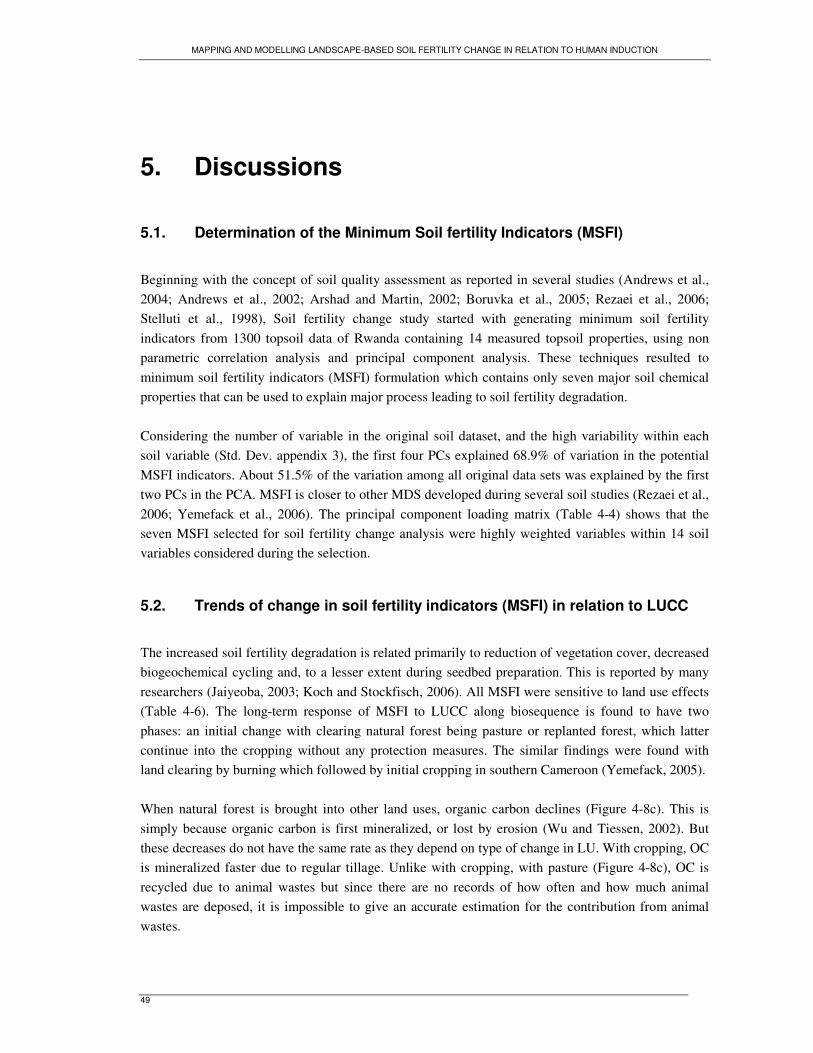
MAPPING AND MODELLING LANDSCAPE-BASED SOIL FERTILITY CHANGE IN RELATION TO HUMAN INDUCTION
49
5. Discussions
5.1. Determination of the Minimum Soil fertility Indicators (MSFI)
Beginning with the concept of soil quality assessment as reported in several studies (Andrews et al., 2004; Andrews et al., 2002; Arshad and Martin, 2002; Boruvka et al., 2005; Rezaei et al., 2006; Stelluti et al., 1998), Soil fertility change study started with generating minimum soil fertility indicators from 1300 topsoil data of Rwanda containing 14 measured topsoil properties, using non parametric correlation analysis and principal component analysis. These techniques resulted to minimum soil fertility indicators (MSFI) formulation which contains only seven major soil chemical properties that can be used to explain major process leading to soil fertility degradation. Considering the number of variable in the original soil dataset, and the high variability within each soil variable (Std. Dev. appendix 3), the first four PCs explained 68.9% of variation in the potential MSFI indicators. About 51.5% of the variation among all original data sets was explained by the first two PCs in the PCA. MSFI is closer to other MDS developed during several soil studies (Rezaei et al., 2006; Yemefack et al., 2006). The principal component loading matrix (Table 4-4) shows that the seven MSFI selected for soil fertility change analysis were highly weighted variables within 14 soil variables considered during the selection.
5.2. Trends of change in soil fertility indicators (MSFI) in relation to LUCC
The increased soil fertility degradation is related primarily to reduction of vegetation cover, decreased biogeochemical cycling and, to a lesser extent during seedbed preparation. This is reported by many researchers (Jaiyeoba, 2003; Koch and Stockfisch, 2006). All MSFI were sensitive to land use effects (Table 4-6). The long-term response of MSFI to LUCC along biosequence is found to have two phases: an initial change with clearing natural forest being pasture or replanted forest, which latter continue into the cropping without any protection measures. The similar findings were found with land clearing by burning which followed by initial cropping in southern Cameroon (Yemefack, 2005). When natural forest is brought into other land uses, organic carbon declines (Figure 4-8c). This is simply because organic carbon is first mineralized, or lost by erosion (Wu and Tiessen, 2002). But these decreases do not have the same rate as they depend on type of change in LU. With cropping, OC is mineralized faster due to regular tillage. Unlike with cropping, with pasture (Figure 4-8c), OC is recycled due to animal wastes but since there are no records of how often and how much animal wastes are deposed, it is impossible to give an accurate estimation for the contribution from animal wastes.
MAPPING AND MODELLING LANDSCAPE-BASED SOIL FERTILITY CHANGE IN RELATION TO HUMAN INDUCTION
50
Highest Al concentrations in pine and agriculture systems were observed at the 30 cm soil depth compared with pasture land (Figure 4-8a). These findings can be explained by the decrease of pH in the same systems; and therefore increases Al solubility in the surface (Lilienfein et al., 2003). In other hand, with the tropical climate, especially in western province of Rwanda, the heavy rains and its different pattern destroy soils which are uncovered. This accelerates the deterioration of silicates and their leaching involves a loss of silica in the soil and the accumulation of oxides of Al and other oxides (Fe and Mn). The increase of Al in agriculture land responds to what is often reported in the literature as leaching effect in tropical soils (Dabin, 1985; Mutwewingabo and Rutunga, 1987), and meets Yemefack (2005) findings. The effect of pasture use on soil fertility was generally small when compared with effects of other permanent cultures like pine plantation because it preserves more nutrients (Figure 4-11b). However, the high available phosphorus in pine plantation can be attributed to the roots activity of pine than for the grass (Table 4-6). Phosphorous that are in accessible areas (in depth) is brought to the surface by roots activities. The availability of phosphorous under forest cover confirmed the conclusions from several experiments that have shown gradual improvement of P in the surface by root activity (Islam and Weil, 2000).
5.3. Performance of SFI model vs to MSFI models
By weighting the minimum soil fertility indicators (MSFI) into score values, SFI index is an additive index which combine the appreciation of each MSFI in term of land productivity and stability, and it is found to be in-line with other indices reported by some researches (Andrews et al., 2003; Andrews et al., 2002; Pervanchon et al., 2005). Of the geostatistical analysis of MSFI and SFI, SFI was the best choice for representing spatial structure of soil fertility and changes that happened due to LUCC in hilly slope condition (Figure 4-14). The relative improvement of SFI over MSFI was consistent and large. The relationship with CLORPT factors remained as it was with MSFI. However, the nugget effect was smaller while in some cases of MSFI (e.g. P, and Al) it was very high. Moreover, the experiment variogram of SFI had bounded sill, which indicates that the noise has indeed been removed. Incorporating soil map and soil predictive components derived from DEM and derived hydrological indices in spatial prediction of SFI gives better results over OK (Figure 4-18). The range parameter of residuals was mush shorter, and nugget was proportionally reduced, indicating that some variations which were not explained by the model fitted using only target variable, has been to some extent explained by soil type and topography. This largely confirms results obtained in other studies on digital soil mapping (McBratney et al., 2003) or mapping soil properties based on multivariate secondary data (Hengl et al., 2004b; Simbahan et al., 2006). The map of SFI generated with RK with SMUs and SPCs reveals the details which can not be seen on SFI map generated using OK. For instance in SE of Gishwati (between 48’ and 50’) Eutropepts was separated to Tropohumults while in OK they merged. Referred to SFI map values (Figure 4-18) also in previous analysis (Table 4-9), Eutropepts had moderate to high SFI value from 6.2 to 6.9 with average value of 6.7 while
MAPPING AND MODELLING LANDSCAPE-BASED SOIL FERTILITY CHANGE IN RELATION TO HUMAN INDUCTION
51
Tropohumults low to moderated SFI (5.5 to 6.2) with average of 6.0. Yet, in the NE (between 42’ and 44’), SFI was underestimated by OK in Eutrandepts (SFI ≤ 5.5) at moderated elevation ( ≈ 2400m) while it was between 5.5 and 6.2 according to RK using SMU and SPCs. The difference remarked between SFI predicted using OK and RK concerned the differentiations of boundaries between polygons drown by soil type and pattern of the topography. OK was found not realistic without considering other predictive factors.
5.4. Degradation of soil fertility in Gishwati highlands
By computing the deviation of SFI from Natural forest being agricultural purpose (referred in this study as DI), permanent pine plantation or pasture reveals the deterioration levels of soil fertility in Gishwati watershed. DI enables us to detect early degradation caused by different land uses in different times since the natural forest conversion (Figure 4-22c). It is discovered that the deterioration occurs in soil quality when natural forest is degraded and converted to agriculture without the use of appropriate soil and water conservation. The same problem was also observed in Bangladesh (Islam and Weil, 2000) where soil under cultivated were high degraded over 20 years. At the same time, if natural forest is converted in forest plantation, the choice of species being planted is outmost important for soil quality conservation. If it was Acacia planted in large extent rather than pine, soils could not be degraded at such alarming rate (-24% refer back to table 4-10 or to the blue area in the figure 4-22c, NE from 42’ to 44’ where DI 5.2−≥ ). This finding joints the experiment done in Bangladesh where soils under reforestation with Acacia, the DI was actually positive (Islam and Weil, 2000). The findings are consistent with other studies on soil fertility declines in the tropics following deforestation and conversion to agricultural lands (Lemenih et al., 2005a). Lower degradation responses following deforestation are common observations in most Andepts (Andaquepts and Eutrandepts). For example in NE of Gishwati study area (between 40’ and 42’ in the map) where land conversion was done at the same time (early 1980s) with same use (pasture) but the deterioration of soil fertility was different (DI 2.1−≤ ) in Eutrandepts (refer back to figure 4-3 and figure 4-22c) and (DI 5.2−≥ ) in Tropohumults. We found that such indicated soils that contain allophanic minerals from volcanic eruptions can be much more resistant to degradation from cultivation than soil derived acidic material (Tropohumults) or from river deposits (Troportents and Tropaquepts). The similar results were observed with Andisols (Parfitt et al., 1997). The Andisol contained allophanes and ferrihydrite whereas the Inceptisols contained mica as the main clay mineral. The samples were taken under perennial pasture and cropped area with cropped with barley and brassica. They found that the stability of organic matter was greater in the Andisol than in the Inceptisol, and it was less likely to be affected by cropping. Allophanes and ferrihydrites appeared to have a stabilizing influence on a large part of the organic matter in the Andisol.

MAPPING AND MODELLING LANDSCAPE-BASED SOIL FERTILITY CHANGE IN RELATION TO HUMAN INDUCTION
52
6. Conclusions and recommendations
6.1. Conclusions
The objective of this study was to quantify the response of soil fertility to human activity in Rwandan highlands using a case study of Gishwati catchment area. We integrated several methodological steps to provide a preliminary framework that can be used to assess and locate soil fertility degradation as one major concern of precision agriculture in Rwanda. We made use of principal component analysis (PCA) and that was applied to the whole dataset of Rwanda in order to determine the Minimum Data Set (MDS) that can be use in soil fertility degradation assessment. Referred in this study as Minimum Soil Fertility Indicators (MSFI); seven major soil chemical properties were selected due to their higher score in two first PCs. Those are pH, OC, Al, P, K, Ca and Mg. With these findings we got the answer of the first question about the Minimum Data Set that can be used to assess the landscape-based soil fertility change in Rwandan highland. Next, we collected 200 soil samples and we revisited 17 soil profiles done in 1981 during soil map project of Rwanda (CPR) in order to assess the early changes in soil fertility. Unfortunately, the previous profiles were few to allow us the chronosequential assessment (Type I) and state with evidence. In this case, we used biosequential or type II data to answer to the part of the second question which was raised as: if there a significant change in soil fertility over the last 25 years. One-way ANOVA revealed that each soil fertility indicator has been heavily affected by land use change over 25 years ( 01.0≤P ). Study on how can the individual indicators of soil fertility be modeled into and integrative measure of soil fertility and fertility degradation as question 3, SFI was developed using an adapted conceptual framework after Andrews at al., 2003. This framework was made malleable using probabilistic approach and generating a score value of each class of soil properties that were already available after Mutwewingabo et al., 1987. Integration of MSFI into index of soil fertility (SFI) enabled us to reasonably interpret the complex data set with conflicting or contradictory trends due to irregular change in CLORPT factors. This strategic method revealed that the loss of soil fertility is higher about 31% when natural forest is converted into pasture and latter continue into cropland. About 24 % of soil fertility is lost with reforestation of cleared natural forest without an appropriate species being planted. Note that pasture conserves more or less soil fertility compared to other land uses. Only 16% is lost in grassland for 25 years since natural forest has been converted. However it has discovered that soils under volcanic material are degraded slowly compared to acidic soils even though they are under same use. Only 7 % of soil fertility is lost after 11 years of regular cultivation. This comes to answer the fourth question to what extent land use change contributes to soil fertility change.
MAPPING AND MODELLING LANDSCAPE-BASED SOIL FERTILITY CHANGE IN RELATION TO HUMAN INDUCTION
53
Geostatistical methods that utilized spatially correlated secondary information (RK) increased the quality of maps of SFI as compared to Ordinary kriging (OK). Both OK and RK yielded lower relative perdition error (36% to 40%). However, Regression kriging using soil predictive components (SPCs) generated from improved DEM with combination of soil type (SMUs) performed better than OK not only in terms of increasing map accuracy but also in visualization of details. In stepwise RK method relative improvement in map accuracy over OK was 4% and there was little loss of accuracy when the model was used to predict SFI at unsampled locations. SPCs was the most valuable and quantitative CLORPT factor for detailed mapping of SFI at watershed level, whereas the SMUs was used to represent parental material which varied from north to south of Gishwati watershed. With SFI map of 2006 we satisfactory answered the firth question on how successfully the spatial pattern of soil fertility can be predicted in complex lithology of Rwandan highlands. The prediction ranged from 91% to 93 % accuracy. However it should be emphasized that a SFI dataset with a fairly equal spreading of point is more appropriate for regression kriging.
6.2. Recommendations
This study was considered as a preliminary quantitative assessment of soil fertility degradation and has involved secondary data unknown accuracy of the producer. We assumed that this secondary data contained uncertainties that may mask relationships with MSFI or SFI. Relying on the secondary information is risky because (i) SPCs used to generated the stepwise regression model may not be coincide exactly to the SFI point for several reasons such as GPS precision and so on, (ii) the range of soil properties classes used to develop SFI may mask the variability which could be highlighted if the range was made shorter. Those errors in the secondary information could propagate significant errors in the SFI prediction. To reduce uncertainties, we recommend updating existing soil map, including detailed geologic map and review existing topographic information by independently measured elevations, before any soil-landscape modelling and prediction. Although CLORPT approach was used in our study, this empirical approach tends to decrease its ability in explaining the variability in the SFI model of spatial dependence. SFI Gaussian model yielded the high nugget effect still after the drifts used were removed. Adding quantitative human disturbance as drift may reduce residuals and consequently reduce unexplained variability. More work need to be done to develop a quantitative predictive component of land use as predictor of human-induced changes, and this may enhance the CLORPT approach in soil fertility change analysis. Next to this study, more research should be devoted to these important topics, in particular validation of usefulness of SFI in decision making and implantation. The similar research should be conducted in different environment to test the transportability of SFI approach. For further understanding of the degradation process, we suggest that long-term monitoring sites should established, regular soil samples and management aspect should be taken and stored in Master database. With such data, the model of temporal change in soil fertility can then be produced and SFI approach can be further improved for regular monitoring of the changes in soil fertility of Rwanda.
MAPPING AND MODELLING LANDSCAPE-BASED SOIL FERTILITY CHANGE IN RELATION TO HUMAN INDUCTION
54
References
ABOS-AGCD, 1983. Fourth international soil classification workshop, ABOS-AGCD, Brussels. Amini, M., Afyuni, M., Fathianpour, N., Khademi, H. and Fluhler, H., 2005. Continuous soil pollution
mapping using fuzzy logic and spatial interpolation. Geoderma, 124(3-4): 223-233. Andrews, S.S., Flora, C.B., Mitchell, J.P. and Karlen, D.L., 2003. Growers' perceptions and
acceptance of soil quality indices. Geoderma, 114(3-4): 187-213. Andrews, S.S., Karlen, D.L. and Cambardella, C.A., 2004. The Soil Management Assessment
Framework: A Quantitative Soil Quality Evaluation Method. Soil Sci Soc Am J, 68(6): 1945-1962.
Andrews, S.S., Karlen, D.L. and Mitchell, J.P., 2002. A comparison of soil quality indexing methods for vegetable production systems in Northern California. Agriculture, Ecosystems & Environment, 90(1): 25-45.
Arshad, M.A. and Martin, S., 2002. Identifying critical limits for soil quality indicators in agro-ecosystems. Agriculture, Ecosystems & Environment, 88(2): 153-160.
Bishop, T.F.A. and McBratney, A.B., 2001. A comparison of prediction methods for the creation of field-extent soil property maps. Geoderma, 103(1-2): 149-160.
Boruvka, L., Vacek, O. and Jehlicka, J., 2005. Principal component analysis as a tool to indicate the origin of potentially toxic elements in soils. Geoderma, 128(3-4): 289-300.
Breuer, L., Huisman, J.A., Keller, T. and Frede, H.G., 2006. Impact of a conversion from cropland to grassland on C and N storage and related soil properties: Analysis of a 60-year chronosequence. Geoderma, 133(1-2): 6-18.
Carroll, Z.L. and Oliver, M.A., 2005. Exploring the spatial relations between soil physical properties and apparent electrical conductivity. Geoderma, 128(3-4): 354-374.
Dabin, B., 1985. Les soils tropicaux acides, Série Pédologie XXI. Cahier de l'ORSTOM 7-19 pp. Dumanski, J. and Pieri, C., 2000. Land quality indicators: research plan. Agriculture, Ecosystems &
Environment, 81(2): 93-102. Goovaerts, P., 1999. Review of Multivariate Geostatistics. 2nd, completely revised edition by Hans
Wackernagel; Springer, Berlin, 1998. Hardcover, 291 pp. ISBN 3-540-64721-x. Geoderma, 93(3-4): 345-347.
Haileslassie, A., Priess, J., Veldkamp, E., Teketay, D. and Lesschen, J.P., 2005. Assessment of soil nutrient depletion and its spatial variability on smallholders' mixed farming systems in Ethiopia using partial versus full nutrient balances. Agriculture, Ecosystems & Environment, 108(1): 1-16.
Hartemink, A.E., 2003. Soil fertility decline in the tropics : with case studies on plantations. CABI, Wallingford etc., 360 p. pp.
Hengl, T., Gruber, S. and Shrestha, D.P., 2003. Digital terrain analysis.lecture notes and user guide ITC, Enschede, the Netherlands, Enschede, 56 pp. Hengl, T., Gruber, S. and Shrestha, D.P., 2004a. Reduction of errors in digital terrain parameters used
in soil-landscape modelling. International Journal of Applied Earth Observation and Geoinformation, 5(2): 97-112.
Hengl, T., Heuvelink, G.B.M. and Stein, A., 2004b. A generic framework for spatial prediction of soil variables based on regression-kriging. Geoderma, 120(1-2): 75-93.
Iqbal, J., Thomasson, J.A., Jenkins, J.N., Owens, P.R. and Whisler, F.D., 2005. Spatial Variability Analysis of Soil Physical Properties of Alluvial Soils. Soil Science Society of America, 69.
Islam, K.R. and Weil, R.R., 2000. Land use effects on soil quality in a tropical forest ecosystem of Bangladesh. Agriculture, Ecosystems & Environment, 79(1): 9-16.
MAPPING AND MODELLING LANDSCAPE-BASED SOIL FERTILITY CHANGE IN RELATION TO HUMAN INDUCTION
55
Jaiyeoba, I.A., 2003. Changes in soil properties due to continuous cultivation in Nigerian semiarid Savannah. Soil and Tillage Research, 70(1): 91-98.
Jetten, V., Govers, G. and Hessel, R., 2003. Erosion models: quality of spatial predictions. Hydrol. Process., 17(5): 887-900.
Jorgensen, S.E., 1994. Models as instruments for combination of ecological theory and environmental practice. Ecological Modelling, 75-76: 5-20.
Karlen, D.L., Ditzler, C.A. and Andrews, S.S., 2003. Soil quality: why and how? Geoderma, 114(3-4): 145-156.
Koch, H.-J. and Stockfisch, N., 2006. Loss of soil organic matter upon ploughing under a loess soil after several years of conservation tillage. Soil and Tillage Research, 86(1): 73-83.
Lagacherie, P. and Voltz, M., 2000. Predicting soil properties over a region using sample information from a mapped reference area and digital elevation data: a conditional probability approach. Geoderma, 97(3-4): 187-208.
Lark, R.M. and Ferguson, R.B., 2004. Mapping risk of soil nutrient deficiency or excess by disjunctive and indicator kriging. Geoderma, 118(1-2): 39-53.
Lemenih, M., Karltun, E. and Olsson, M., 2005a. Assessing soil chemical and physical property responses to deforestation and subsequent cultivation in smallholders farming system in Ethiopia. Agriculture, Ecosystems & Environment, 105(1-2): 373-386.
Lemenih, M., Karltun, E. and Olsson, M., 2005b. Soil organic matter dynamics after deforestation along a farm field chronosequence in southern highlands of Ethiopia. Agriculture, Ecosystems & Environment, 109(1-2): 9-19.
Li, W., Zhang, C., Burt, J.E., Zhu, A.X. and Feyen, J., 2004. Two-dimensional Markov Chain Simulation of Soil Type Spatial Distribution. Soil Sci Soc Am J, 68(5): 1479-1490.
Lilienfein, J. et al., 2003. Soil Fertility under Native Cerrado and Pasture in the Brazilian Savanna. Soil Sci Soc Am J, 67(4): 1195-1205.
Liu, T.-L., Juang, K.-W. and Lee, D.-Y., 2006. Interpolating Soil Properties Using Kriging Combined with Categorical Information of Soil Maps. Soil Sci Soc Am J, 70(4): 1200-1209.
McBratney, A.B., Mendonca Santos, M.L. and Minasny, B., 2003. On digital soil mapping. Geoderma, 117(1-2): 3-52.
McBratney, A.B., Odeh, I.O.A., Bishop, T.F.A., Dunbar, M.S. and Shatar, T.M., 2000. An overview of pedometric techniques for use in soil survey. Geoderma, 97(3-4): 293-327.
MINITERRE/Rwanda, 2003. National strategy and action plan for the conservation of biodiversity in Rwanda, MINITERRE, Kigali.
MINITERRE/Rwanda, 2005. Initial national communication under the United Nations framework convention on climate change, MINITERRE, Kigali.
Moeyersons, J., 2003. The topographic thresholds of hillslope incisions in southwestern Rwanda. CATENA, 50(2-4): 381-400.
Mueller, T.G. and Pierce, F.J., 2003. Soil Carbon Maps: Enhancing Spatial Estimates with Simple Terrain Attributes at Multiple Scales. Soil Sci Soc Am J, 67(1): 258-267.
Mueller, T.G., Pierce, F.J., Schabenberger, O. and Warncke, D.D., 2001. Map Quality for Site-Specific Fertility Management. Soil Sci Soc Am J, 65(5): 1547-1558.
Mueller, T.G., Pusuluri, N.B., Mathias, K.K., Cornelius, P.L. and Barnhisel, R.I., 2004a. Site-Specific Soil Fertility Management: A Model for Map Quality. Soil Sci Soc Am J, 68(6): 2031-2041.
Mueller, T.G. et al., 2004b. Map Quality for Ordinary Kriging and Inverse Distance Weighted Interpolation. Soil Sci Soc Am J, 68(6): 2042-2047.
Mukashema, A., 2003. Evaluation de la fertilite des sols et son impact sur la production du cafeier arabica dans le District de Maraba. Ir. Thesis, Universite Nationale du Rwanda (UNR), Butare, 195 pp.
Mutwewingabo, B., 1984. Pédologie et micro morphologie de trois toposéquences des sols à horizon sombre de profondeur de Gikongoro et de deux pédons Butare (Rwanda). Isothermes et caractéristiques d’absorption du phosphate par ces sols. Thèse de doctorat Thesis, Université de Laval, Canada, 114 pp.
MAPPING AND MODELLING LANDSCAPE-BASED SOIL FERTILITY CHANGE IN RELATION TO HUMAN INDUCTION
56
Mutwewingabo, B. and Rutunga, V., 1987. Etude des sols des stations d’essais du projet d’intensification de l’agriculture Gikongoro(PIA)
Neel, H.H., Prins, D. and E.Vindervogel, 1976. Etude de la fertilité des sols à l’aide des vases de végétation ISAR, ISAR-RUBONA, Butare.
Ntaneza, D., 1988. Examen de la fertilité des sols des périmètres semenciers de Bumbogo et Rubungo au Rwanda. Msc Thesis, Université Laval, Canada, 194 pp.
Parfitt, R.L., Theng, B.K.G., Whitton, J.S. and Shepherd, T.G., 1997. Effects of clay minerals and land use on organic matter pools. Geoderma, 75(1-2): 1-12.
Park, S.J. and Vlek, P.L.G., 2002. Environmental correlation of three-dimensional soil spatial variability: a comparison of three adaptive techniques. Geoderma, 109(1-2): 117-140.
Pennock, D.J. and Veldkamp, A., 2006. Advances in landscape-scale soil research. Geoderma, 133(1-2): 1-5.
Pervanchon, F. et al., 2005. A novel indicator of environmental risks due to nitrogen management on grasslands. Agriculture, Ecosystems & Environment, 105(1-2): 1-16.
Plumptre, A.J., Masozera, M. and Vedder, A., 2001. The Impact of Civil War on the Conservation of Protected Areas in Rwanda. 33.
Rezaei, S.A., Gilkes, R.J. and Andrews, S.S., 2006. A minimum data set for assessing soil quality in rangelands. Geoderma, 136(1-2): 229-234.
Sena, M.M., Frighetto, R.T.S., Valarini, P.J., Tokeshi, H. and Poppi, R.J., 2002. Discrimination of management effects on soil parameters by using principal component analysis: a multivariate analysis case study. Soil and Tillage Research, 67(2): 171-181.
Shrestha, D.P., Zinck, J.A. and Van Ranst, E., 2004. Modelling land degradation in the Nepalese Himalaya. CATENA, 57(2): 135-156.
Simbahan, G.C., Dobermann, A., Goovaerts, P., Ping, J. and Haddix, M.L., 2006. Fine-resolution mapping of soil organic carbon based on multivariate secondary data. Geoderma, 132(3-4): 471-489.
Sonneveld, M.P.W., Schoorl, J.M. and Veldkamp, A., 2006. Mapping hydrological pathways of phosphorus transfer in apparently homogeneous landscapes using a high-resolution DEM. Geoderma, 133(1-2): 32-42.
Srivastava, R. and Saxena, R.K., 2004. Technique of large-scale soil mapping in basaltic terrain using satellite remote sensing data. International Journal of Remote Sensing, 25(4): 679-688.
Stelluti, M., Maiorana, M. and De Giorgio, D., 1998. Multivariate approach to evaluate the penetrometer resistance in different tillage systems. Soil and Tillage Research, 46(3-4): 145-151.
Thompson, J.A., Pena-Yewtukhiw, E.M. and Grove, J.H., 2006. Soil-landscape modeling across a physiographic region: Topographic patterns and model transportability. Geoderma, 133(1-2): 57-70.
Tomer, M.D. and James, D.E., 2004. Do Soil Surveys and Terrain Analyses Identify Similar Priority Sites for Conservation? Soil Sci Soc Am J, 68(6): 1905-1915.
Verdoodt, A., 2003. Elaboration and Application of an Adjusted Agricultural Land Evaluation Model for Rwanda. Ph.D Thesis, Gent University, Gent, 441 pp.
Verdoodt, A. and Van Ranst, E., 2006. Environmental assessment tools for multi-scale land resources information systems: A case study of Rwanda. Agriculture, Ecosystems & Environment, 114(2-4): 170-184.
Wang, X. and Gong, Z., 1998. Assessment and analysis of soil quality changes after eleven years of reclamation in subtropical China. Geoderma, 81(3-4): 339-355.
Webster, R., 2000. Is soil variation random? Geoderma, 97(3-4): 149-163. Wu, R. and Tiessen, H., 2002. Effect of Land Use on Soil Degradation in Alpine Grassland Soil,
China. Soil Sci Soc Am J, 66(5): 1648-1655. Yemefack, M., 2005. Modelling and Monitoring Soil and Land Use Dynamics:Within Shifting
Agricultural Landscape Mosaic Systems in Southern Cameroon. Dissertation Thesis, ITC Enschede and Utrecht University, The netherlands, 194 pp.

MAPPING AND MODELLING LANDSCAPE-BASED SOIL FERTILITY CHANGE IN RELATION TO HUMAN INDUCTION
57
Yemefack, M., Jetten, V.G. and Rossiter, D.G., 2006. Developing a minimum data set for characterizing soil dynamics in shifting cultivation systems. Soil and Tillage Research, 86(1): 84-98.
Yemefack, M., Rossiter, D.G. and Njomgang, R., 2005. Multi-scale characterization of soil variability within an agricultural landscape mosaic system in southern Cameroon. Geoderma, 125(1-2): 117-143.
Zaag, V.D., 1981. La fertilité des sols du Rwanda, ISAR-RUBONA Butare. Zaag, V.D., V., R. and B., M., 1982. La fertilité des sols au Rwanda Ziadat, F.M., 2005. Analyzing Digital Terrain Attributes to Predict Soil Attributes for a Relatively
Large Area. Soil Sci Soc Am J, 69(5): 1590-1599.

MA
PP
ING
AN
D M
OD
ELL
ING
LA
ND
SC
AP
E-B
AS
ED
SO
IL F
ER
TIL
ITY
CH
AN
GE
IN R
ELA
TIO
N T
O H
UM
AN
IND
UC
TIO
N
58
App
endi
ces
App
endi
x 1:
Fie
ld-D
ata
Col
lect
ion
Form
for
Soil
Fert
ility
Map
ping
and
Mod
ellin
g Id
entif
icat
ion
of th
e sa
mpl
e si
te
Lan
d U
se a
nd L
and
cove
r cha
nge
Fe
rtili
zatio
n E
rosi
on a
nd c
onse
rvat
ion
prac
tices
ID
N
ame
of th
e si
te
X
Y LP
P
LU
LC /G
C
TC
DC
F
T P
F
EF
E
D
EC
P
1
2
3
4
5
6
7
8
ID: S
ampl
e id
entif
ier
X
: Lon
gitu
de (d
ecim
al d
egre
es)
Y
: Lat
itude
(dec
imal
deg
rees
)
LP:
Lan
dsca
pe p
ositi
on
1=
Sum
mit
2=
uppe
r slo
pe
3=M
iddl
e sl
ope
4=
low
er s
lope
5=
Val
ley
PL
U: P
rese
nt L
and
Use
: 1=A
gric
ultu
re
2=P
astu
re
3=Fo
rest
pla
ntat
ion
4=
Nat
ural
fore
st 5
=Agr
ofor
estr
y (i
f dom
inan
t)
LC
/GC
: Lan
d /G
roun
d C
over
: 1=C
rops
2=
Eve
rgre
en tr
ees
(>5m
hei
ght)
3
=Dec
iduo
us tr
ees
(>5m
hei
ght
4=S
hrub
s (<
5m h
eigh
t)
5=G
rass
es
TC
: Typ
e of
cha
nge
0=
No
chan
ge/ N
atur
al fo
rest
1=
Nat
ural
fore
st to
cro
plan
d 2=
Nat
ural
fore
st to
Pas
ture
3=
Past
ure
to C
ropl
and
4
=N
atur
al fo
rest
to fo
rest
pla
ntat
ion
DC
: Dat
e of
Con
vers
ion
(yea
r)
FT
: Fer
tiliz
atio
n T
ype:
1=o
rgan
ic 2
=min
eral
(spe
cify
) P
F: L
ast p
erio
d of
fert
iliza
tion
(yea
r)
EF:
Ero
sion
Fea
ture
s: 0
= N
o er
osio
n 1
=Spl
ash
2=R
ill
3=G
ully
4=
Lan
dslid
e E
D: E
rosi
on d
ensi
ty (%
of c
over
age)
E
CP:
0=N
on e
rosi
on c
ontr
ol
1=fo
sses
2=
Agr
ofor
estr
y
3=Fa
llow
4=
Mul
chin
g
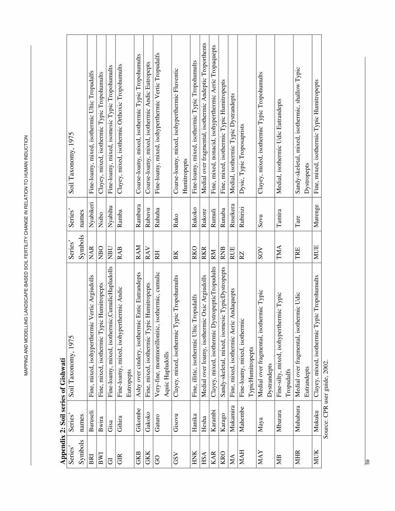
MA
PP
ING
AN
D M
OD
ELL
ING
LA
ND
SC
AP
E-B
AS
ED
SO
IL F
ER
TIL
ITY
CH
AN
GE
IN R
ELA
TIO
N T
O H
UM
AN
IND
UC
TIO
N
59
App
endi
x 2:
Soi
l ser
ies o
f Gis
hwat
i Se
ries
’ Sy
mbo
ls
Seri
es’
nam
es
Soil
Tax
onom
y, 1
975
Seri
es’
Sym
bols
Se
ries
’ na
mes
So
il T
axon
omy,
197
5
BR
I B
urus
eli
Fine
, mix
ed, i
sohy
pert
herm
ic V
ertic
Arg
iudo
lls
NA
R
Nya
bike
ri
Fine
-loam
y, m
ixed
, iso
ther
mic
Ulti
c T
ropu
dalfs
BW
I B
wir
a Fi
ne, m
ixed
, iso
ther
mic
Typ
ic H
umitr
opep
ts
NB
O
Nsi
bo
Cla
yey,
mix
ed, i
soth
erm
ic T
ypic
Tro
pohu
mul
ts
GI
Gis
a Fi
ne-lo
amy,
mix
ed, i
soth
erm
ic,C
umul
icH
aplu
dolls
N
BU
N
yabi
hu
Fine
-loam
y, m
ixed
, iso
mes
ic T
ypic
Tro
pohu
mul
ts
GIR
G
ihir
a Fi
ne-lo
amy,
mix
ed, i
sohy
pert
herm
ic A
ndic
E
utro
pept
s R
AB
R
amba
C
laye
y, m
ixed
, iso
ther
mic
Ort
hoxi
c T
ropo
hum
ults
GK
B
Gik
ombe
A
shy
over
cin
dery
, iso
ther
mic
Ent
ic E
utra
ndep
ts
RA
M
Ram
bura
C
oars
e-lo
amy,
mix
ed, i
soth
erm
ic T
ypic
Tro
pohu
mul
ts
GK
K
Gak
oko
Fine
, mix
ed, i
soth
erm
ic T
ypic
Hum
itrop
epts
R
AV
R
ubav
u C
oars
e-lo
amy,
mix
ed, i
soth
erm
ic A
ndic
Eut
rope
pts
GO
G
atur
o V
ery-
fine,
mon
tmor
illon
itic,
isot
herm
ic, c
umul
ic
Aqu
ic H
aplu
dolls
R
H
Ruh
uha
Fine
-loam
y, m
ixed
, iso
hype
rthe
rmic
Ver
tic T
ropu
dalfs
GSV
G
isov
u C
laye
y, m
ixed
, iso
ther
mic
Typ
ic T
ropo
hum
ults
R
K
Ruk
o C
oars
e-lo
amy,
mix
ed, i
sohy
pert
herm
ic F
luve
ntic
H
umitr
opep
ts
HN
K
Han
ika
Fine
, illi
tic, i
soth
erm
ic U
ltic
Tro
puda
lfs
RK
O
Ruk
oko
Fine
-loam
y, m
ixed
, iso
ther
mic
Typ
ic T
ropo
hum
ults
H
SA
Hes
ha
Med
ial o
ver l
oam
y, is
othe
rmic
Oxi
c A
rgiu
dolls
R
KR
R
ukor
e M
edia
l ove
r fra
gmen
tal,
isot
herm
ic A
ndep
tic T
ropo
rthe
nts
KA
R
Kar
ambi
C
laye
y, m
ixed
, iso
ther
mic
Dys
trop
eptic
Tro
pudu
lts
RM
R
umul
i Fi
ne, m
ixed
, non
acid
, iso
hype
rthe
rmic
Aer
ic T
ropa
quep
ts
KR
O
Kar
ago
Sand
y-sk
elet
al, m
ixed
, iso
mes
ic T
ypic
Dys
trop
epts
R
NB
R
unab
a Fi
ne, m
ixed
, iso
ther
mic
Typ
ic H
umitr
opep
ts
MA
M
ukam
ira
Fine
, mix
ed, i
soth
erm
ic A
eric
And
aque
pts
RU
E
Rus
eker
a M
edia
l, is
othe
rmic
Typ
ic D
ystr
ande
pts
MA
H
Mah
embe
Fi
ne-lo
amy,
mix
ed, i
soth
erm
ic
Typ
icH
umitr
opep
ts
RZ
Rub
iriz
i D
ysic
, Typ
ic T
ropo
sapr
ists
MA
Y
May
a M
edia
l ove
r fra
gmen
tal,
isot
herm
ic T
ypic
D
ystr
ande
pts
SOV
So
vu
Cla
yey,
mix
ed, i
soth
erm
ic T
ypic
Tro
pohu
mul
ts
MB
M
bara
ra
Fine
-silt
y, m
ixed
, iso
hype
rthe
rmic
Typ
ic
Tro
puda
lfs
TM
A
Tam
ira
Med
ial,
isot
herm
ic U
dic
Eut
rand
epts
MH
R
Muh
abur
a M
edia
l ove
r fra
gmen
tal,
isot
herm
ic U
dic
Eut
rand
epts
T
RE
T
are
Sand
y-sk
elet
al, m
ixed
, iso
ther
mic
, sha
llow
Typ
ic
Dys
trop
epts
M
UK
M
ukuk
u C
laye
y, m
ixed
, iso
ther
mic
Typ
ic T
ropo
hum
ults
M
UE
M
uren
ge
Fine
, mix
ed, i
soth
erm
ic T
ypic
Hum
itrop
epts
Sour
ce: C
PR u
ser g
uide
, 200
2.
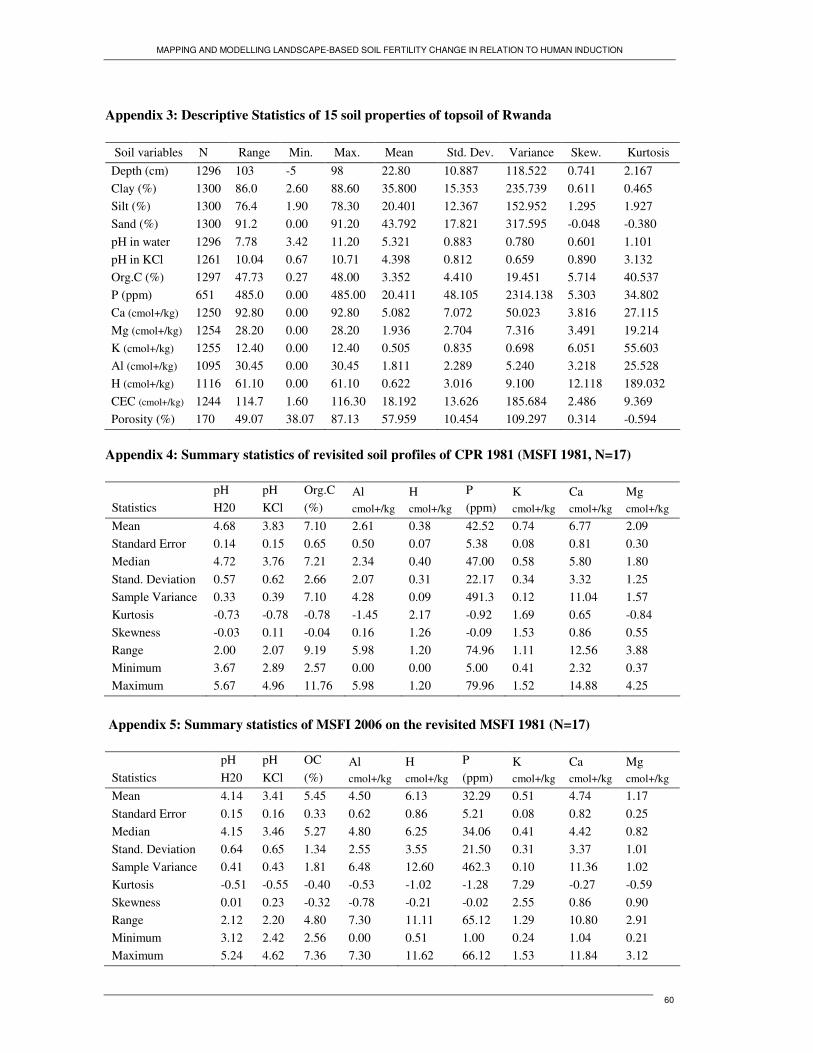
MAPPING AND MODELLING LANDSCAPE-BASED SOIL FERTILITY CHANGE IN RELATION TO HUMAN INDUCTION
60
Appendix 3: Descriptive Statistics of 15 soil properties of topsoil of Rwanda Soil variables N Range Min. Max. Mean Std. Dev. Variance Skew. Kurtosis Depth (cm) 1296 103 -5 98 22.80 10.887 118.522 0.741 2.167 Clay (%) 1300 86.0 2.60 88.60 35.800 15.353 235.739 0.611 0.465 Silt (%) 1300 76.4 1.90 78.30 20.401 12.367 152.952 1.295 1.927 Sand (%) 1300 91.2 0.00 91.20 43.792 17.821 317.595 -0.048 -0.380 pH in water 1296 7.78 3.42 11.20 5.321 0.883 0.780 0.601 1.101 pH in KCl 1261 10.04 0.67 10.71 4.398 0.812 0.659 0.890 3.132 Org.C (%) 1297 47.73 0.27 48.00 3.352 4.410 19.451 5.714 40.537 P (ppm) 651 485.0 0.00 485.00 20.411 48.105 2314.138 5.303 34.802 Ca (cmol+/kg) 1250 92.80 0.00 92.80 5.082 7.072 50.023 3.816 27.115 Mg (cmol+/kg) 1254 28.20 0.00 28.20 1.936 2.704 7.316 3.491 19.214 K (cmol+/kg) 1255 12.40 0.00 12.40 0.505 0.835 0.698 6.051 55.603 Al (cmol+/kg) 1095 30.45 0.00 30.45 1.811 2.289 5.240 3.218 25.528 H (cmol+/kg) 1116 61.10 0.00 61.10 0.622 3.016 9.100 12.118 189.032 CEC (cmol+/kg) 1244 114.7 1.60 116.30 18.192 13.626 185.684 2.486 9.369 Porosity (%) 170 49.07 38.07 87.13 57.959 10.454 109.297 0.314 -0.594
Appendix 4: Summary statistics of revisited soil profiles of CPR 1981 (MSFI 1981, N=17)
Statistics pH H20
pH KCl
Org.C (%)
Al cmol+/kg
H cmol+/kg
P (ppm)
K cmol+/kg
Ca cmol+/kg
Mg cmol+/kg
Mean 4.68 3.83 7.10 2.61 0.38 42.52 0.74 6.77 2.09 Standard Error 0.14 0.15 0.65 0.50 0.07 5.38 0.08 0.81 0.30 Median 4.72 3.76 7.21 2.34 0.40 47.00 0.58 5.80 1.80 Stand. Deviation 0.57 0.62 2.66 2.07 0.31 22.17 0.34 3.32 1.25 Sample Variance 0.33 0.39 7.10 4.28 0.09 491.3 0.12 11.04 1.57 Kurtosis -0.73 -0.78 -0.78 -1.45 2.17 -0.92 1.69 0.65 -0.84 Skewness -0.03 0.11 -0.04 0.16 1.26 -0.09 1.53 0.86 0.55 Range 2.00 2.07 9.19 5.98 1.20 74.96 1.11 12.56 3.88 Minimum 3.67 2.89 2.57 0.00 0.00 5.00 0.41 2.32 0.37 Maximum 5.67 4.96 11.76 5.98 1.20 79.96 1.52 14.88 4.25
Appendix 5: Summary statistics of MSFI 2006 on the revisited MSFI 1981 (N=17)
Statistics pH H20
pH KCl
OC (%)
Al cmol+/kg
H cmol+/kg
P (ppm)
K cmol+/kg
Ca cmol+/kg
Mg cmol+/kg
Mean 4.14 3.41 5.45 4.50 6.13 32.29 0.51 4.74 1.17 Standard Error 0.15 0.16 0.33 0.62 0.86 5.21 0.08 0.82 0.25 Median 4.15 3.46 5.27 4.80 6.25 34.06 0.41 4.42 0.82 Stand. Deviation 0.64 0.65 1.34 2.55 3.55 21.50 0.31 3.37 1.01 Sample Variance 0.41 0.43 1.81 6.48 12.60 462.3 0.10 11.36 1.02 Kurtosis -0.51 -0.55 -0.40 -0.53 -1.02 -1.28 7.29 -0.27 -0.59 Skewness 0.01 0.23 -0.32 -0.78 -0.21 -0.02 2.55 0.86 0.90 Range 2.12 2.20 4.80 7.30 11.11 65.12 1.29 10.80 2.91 Minimum 3.12 2.42 2.56 0.00 0.51 1.00 0.24 1.04 0.21 Maximum 5.24 4.62 7.36 7.30 11.62 66.12 1.53 11.84 3.12
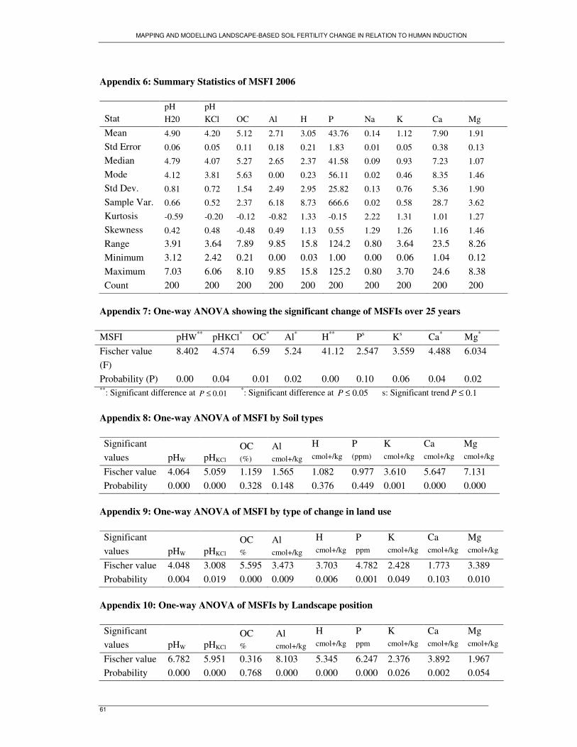
MAPPING AND MODELLING LANDSCAPE-BASED SOIL FERTILITY CHANGE IN RELATION TO HUMAN INDUCTION
61
Appendix 6: Summary Statistics of MSFI 2006
Stat pH H20
pH KCl OC Al H P Na K Ca Mg
Mean 4.90 4.20 5.12 2.71 3.05 43.76 0.14 1.12 7.90 1.91
Std Error 0.06 0.05 0.11 0.18 0.21 1.83 0.01 0.05 0.38 0.13 Median 4.79 4.07 5.27 2.65 2.37 41.58 0.09 0.93 7.23 1.07
Mode 4.12 3.81 5.63 0.00 0.23 56.11 0.02 0.46 8.35 1.46 Std Dev. 0.81 0.72 1.54 2.49 2.95 25.82 0.13 0.76 5.36 1.90
Sample Var. 0.66 0.52 2.37 6.18 8.73 666.6 0.02 0.58 28.7 3.62
Kurtosis -0.59 -0.20 -0.12 -0.82 1.33 -0.15 2.22 1.31 1.01 1.27 Skewness 0.42 0.48 -0.48 0.49 1.13 0.55 1.29 1.26 1.16 1.46
Range 3.91 3.64 7.89 9.85 15.8 124.2 0.80 3.64 23.5 8.26 Minimum 3.12 2.42 0.21 0.00 0.03 1.00 0.00 0.06 1.04 0.12 Maximum 7.03 6.06 8.10 9.85 15.8 125.2 0.80 3.70 24.6 8.38 Count 200 200 200 200 200 200 200 200 200 200
Appendix 7: One-way ANOVA showing the significant change of MSFIs over 25 years MSFI pHW** pHKCl* OC* Al* H** Ps Ks Ca* Mg* Fischer value (F)
8.402 4.574 6.59 5.24 41.12 2.547 3.559 4.488 6.034
Probability (P) 0.00 0.04 0.01 0.02 0.00 0.10 0.06 0.04 0.02 **: Significant difference at 01.0≤P *: Significant difference at 05.0≤P s: Significant trend 1.0≤P
Appendix 8: One-way ANOVA of MSFI by Soil types Significant values pHW pHKCl
OC (%)
Al cmol+/kg
H cmol+/kg
P (ppm)
K cmol+/kg
Ca cmol+/kg
Mg cmol+/kg
Fischer value 4.064 5.059 1.159 1.565 1.082 0.977 3.610 5.647 7.131 Probability 0.000 0.000 0.328 0.148 0.376 0.449 0.001 0.000 0.000
Appendix 9: One-way ANOVA of MSFI by type of change in land use Significant values pHW pHKCl
OC %
Al cmol+/kg
H cmol+/kg
P ppm
K cmol+/kg
Ca cmol+/kg
Mg cmol+/kg
Fischer value 4.048 3.008 5.595 3.473 3.703 4.782 2.428 1.773 3.389 Probability 0.004 0.019 0.000 0.009 0.006 0.001 0.049 0.103 0.010
Appendix 10: One-way ANOVA of MSFIs by Landscape position Significant values pHW pHKCl
OC %
Al cmol+/kg
H cmol+/kg
P ppm
K cmol+/kg
Ca cmol+/kg
Mg cmol+/kg
Fischer value 6.782 5.951 0.316 8.103 5.345 6.247 2.376 3.892 1.967 Probability 0.000 0.000 0.768 0.000 0.000 0.000 0.026 0.002 0.054
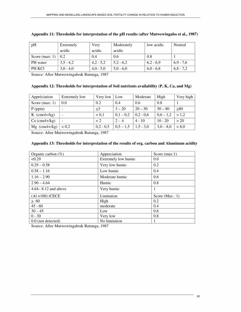
MAPPING AND MODELLING LANDSCAPE-BASED SOIL FERTILITY CHANGE IN RELATION TO HUMAN INDUCTION
62
Appendix 11: Thresholds for interpretation of the pH results (after Mutwewingabo et al., 1987) pH Extremely
acidic Very acidic
Moderately acidic
low acidic Neutral
Score (max: 1) 0.2 0.4 0.6 0.8 1 PH water 3,5 - 4,2 4,2 - 5,2 5,2 - 6,2 6,2 - 6,9 6,9 - 7,6 PH KCl 3,0 - 4,0 4,0 - 5,0 5,0 - 6,0 6,0 - 6,8 6,8 - 7,2 Source: After Mutwewingabo& Rutunga, 1987 Appendix 12: Thresholds for interpretation of Soil nutrients availability (P, K, Ca, and Mg) Appréciation Extremely low Very low Low Moderate High Very high Score (max: 1) 0.0 0.2 0.4 0.6 0.8 1 P (ppm) - <3 3 – 20 20 – 50 50 – 80 >80 K (cmol+/kg) - < 0,1 0,1 – 0,2 0,2 - 0,6 0,6 – 1,2 > 1,2 Ca (cmol+/kg) - < 2 2 - 4 4 - 10 10 - 20 > 20 Mg (cmol+/kg) < 0,2 0,2 - 0,5 0,5 – 1,5 1,5 - 3,0 3,0 – 8,0 > 8,0 Source: After Mutwewingabo& Rutunga, 1987 Appendix 13: Thresholds for interpretation of the results of org. carbon and Aluminum acidity Organic carbon (%) Appreciation Score (max:1) <0.29 Extremely low humic 0.0 0.29 – 0.58 Very low humic 0.2 0.58 – 1.16 Low humic 0.4 1.16 – 2.90 Moderate humic 0.6 2.90 – 4.64 Humic 0.8 4.64– 8.12 and above Very humic 1
(Al ×100) /CECE Limitation Score (Max : 1) > 60 High 0.2 45 - 60 moderate 0.4 30 – 45 Low 0.6 0 - 30 Very low 0.8 0.0 (not detected) No limitation 1 Source: After Mutwewingabo& Rutunga, 1987
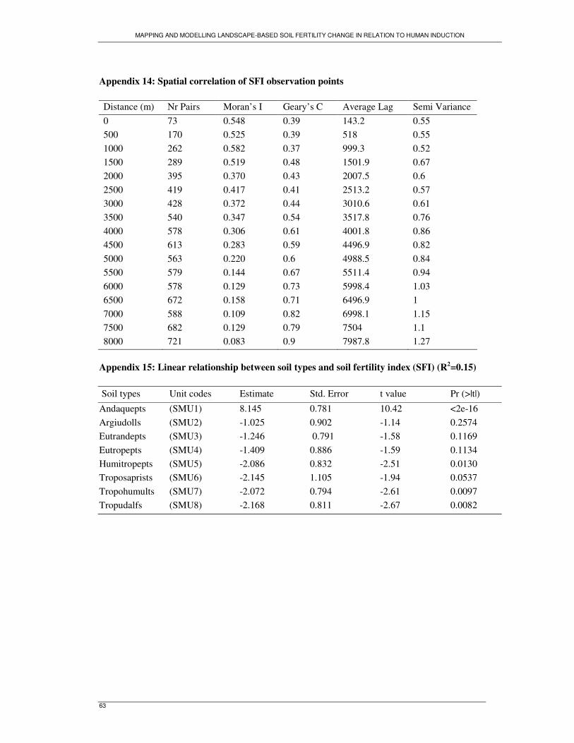
MAPPING AND MODELLING LANDSCAPE-BASED SOIL FERTILITY CHANGE IN RELATION TO HUMAN INDUCTION
63
Appendix 14: Spatial correlation of SFI observation points Distance (m) Nr Pairs Moran’s I Geary’s C Average Lag Semi Variance 0 73 0.548 0.39 143.2 0.55 500 170 0.525 0.39 518 0.55 1000 262 0.582 0.37 999.3 0.52 1500 289 0.519 0.48 1501.9 0.67 2000 395 0.370 0.43 2007.5 0.6 2500 419 0.417 0.41 2513.2 0.57 3000 428 0.372 0.44 3010.6 0.61 3500 540 0.347 0.54 3517.8 0.76 4000 578 0.306 0.61 4001.8 0.86 4500 613 0.283 0.59 4496.9 0.82 5000 563 0.220 0.6 4988.5 0.84 5500 579 0.144 0.67 5511.4 0.94 6000 578 0.129 0.73 5998.4 1.03 6500 672 0.158 0.71 6496.9 1 7000 588 0.109 0.82 6998.1 1.15 7500 682 0.129 0.79 7504 1.1 8000 721 0.083 0.9 7987.8 1.27
Appendix 15: Linear relationship between soil types and soil fertility index (SFI) (R2=0.15)
Soil types Unit codes Estimate Std. Error t value Pr (>|t|)
Andaquepts (SMU1) 8.145 0.781 10.42 <2e-16 Argiudolls (SMU2) -1.025 0.902 -1.14 0.2574 Eutrandepts (SMU3) -1.246 0.791 -1.58 0.1169 Eutropepts (SMU4) -1.409 0.886 -1.59 0.1134 Humitropepts (SMU5) -2.086 0.832 -2.51 0.0130 Troposaprists (SMU6) -2.145 1.105 -1.94 0.0537 Tropohumults (SMU7) -2.072 0.794 -2.61 0.0097 Tropudalfs (SMU8) -2.168 0.811 -2.67 0.0082