mapping tree and shrub leaf area indices in an ombrotrophic

t 109 (2007) 342–360www.elsevier.com/locate/rse

Remote Sensing of Environmen

Mapping tree and shrub leaf area indices in an ombrotrophic peatlandthrough multiple endmember spectral unmixing

O. Sonnentag a,⁎, J.M. Chen a,1, D.A. Roberts b,2, J. Talbot c,3, K.Q. Halligan b,2, A. Govind a,1

a University of Toronto, Department of Geography and Planning, St. George Campus, Sidney Smith Hall,100 St. George St., Room 5047, Toronto, ON, Canada M5S 3G3

b University of California Santa Barbara, Department of Geography, 3611 Ellison Hall, Santa Barbara, CA, 93106-4060, USAc McGill University, Department of Geography, Burnside Hall, 805 Sherbrooke West, Room 705, Montreal, QC, Canada H3A 2K6

Received 12 October 2006; received in revised form 8 January 2007; accepted 13 January 2007

Abstract

Leaf area index (LAI) is an important parameter used by most process-oriented ecosystem models. LAI of forest ecosystems has routinely beenmapped using spectral vegetation indices (SVI) derived from remote sensing imagery. The application of SVI-based approaches to map LAI inpeatlands presents a challenge, mainly due to peatlands characteristic multi-layer canopy comprising shrubs and open, discontinuous tree canopiesunderlain by a continuous ground cover of different moss species, which reduces the greenness contrast between the canopy and the background.

Our goal is to develop a methodology to map tree and shrub LAI in peatlands and similar ecosystems based on multiple endmember spectralmixture analysis (MESMA). This new mapping method is validated using LAI field measurements from a precipitation-fed (ombrotrophic)peatland near Ottawa, Ontario, Canada. We demonstrate first that three commonly applied SVI are not suitable for tree and shrub LAI mapping inombrotrophic peatlands. Secondly, we demonstrate for a three-endmember model the limitations of traditional linear spectral mixture analysis(SMA) due to the unique and widely varying spectral characteristics of Sphagnum mosses, which are significantly different from vascular plants.Next, by using a geometric-optical radiative transfer model, we determine the nature of the equation describing the empirical relationship betweenshadow fraction and tree LAI using nonlinear ordinary least square (OLS) regression. We then apply this equation to describe the empiricalrelationships between shadow and shrub fractions obtained from mixture decomposition with SMA and MESMA, respectively, and tree and shrubLAI, respectively. Less accurate fractions obtained from SMA result in weaker relationships between shadow fraction and tree LAI (R2=0.61) andshrub fraction and shrub LAI (R2=0.49) compared to the same relationships based on fractions obtained from MESMA with R2=0.75 andR2=0.68, respectively. Cross-validation of tree LAI (R2=0.74; RMSE=0.48) and shrub LAI (R2=0.68; RMSE=0.42) maps using fractions fromMESMA shows the suitability of this approach for mapping tree and shrub LAI in ombrotrophic peatlands. The ability to account for a spectrallyvarying, unique Sphagnum moss ground cover during mixture decomposition and a two layer canopy is particularly important.© 2007 Elsevier Inc. All rights reserved.

Keywords: Leaf area index; LAI-2000; Peatlands; Spectral mixture analysis; SMA; MESMA

1. Introduction

Peatlands, which are wetlands that accumulate partiallydecayed plant matter as peat, are an extensive component ofboreal and subarctic ecozones. In Canada, they cover about 14%

⁎ Corresponding author. Tel.: +1 416 946 7715; fax: +1 416 946 3886.E-mail address: [email protected] (O. Sonnentag).

1 Tel.: +1 416 946 7715; fax: +1 416 946 3886.2 Tel.: +1 805 893 2276.3 Tel.: +1 514 398 4111.

0034-4257/$ - see front matter © 2007 Elsevier Inc. All rights reserved.doi:10.1016/j.rse.2007.01.010

of the land area (Tarnocai et al., 2000). Bogs are common typesof peatlands which are precipitation-fed (ombrotrophic) andgenerally lack any other hydrological inputs, resulting in acidicand nutrient-poor conditions. The characteristic multi-layercanopy of bogs comprises a Sphagnum moss ground coverunder ericaceous shrubs, and patches of sparse coniferous trees.Due to this vertical vegetation structure, a substantial proportionof the solar energy reaches the shrub canopy resulting in asignificant role for shrubs in carbon, water, and energyexchanges with the atmosphere (e.g., Baldocchi et al., 2000;Lafleur et al., 2005; Moore et al., 2002).

mailto:[email protected]

http://dx.doi.org/10.1016/j.rse.2007.01.010

343O. Sonnentag et al. / Remote Sensing of Environment 109 (2007) 342–360

Peat accumulation is the result of net primary productivity(NPP), the net gain of carbon in the form of biomass throughphotosynthesis, persistently exceeding the decomposition oforganic matter. Peatlands act as long term stores of carbon withan average long-term apparent carbon accumulation rate of 15–30 g C m−2 year−1 (Turunen et al., 2002). As a result, peatlandsstore up to 450 Gt C or one third of the global soil carbon(Gorham, 1991; Turunen et al., 2002). The role of peatlands aslong-term carbon sinks in the global carbon cycle is closelyrelated to climatic conditions. Possible responses of peatlands toclimatic changes might include shifts in peatland distribution andextent, and a switch from long-term sinks to long-term sources ofatmospheric carbon (e.g., Gorham, 1991; Moore et al., 1998).

A promising means to quantify possible responses of peatlandcarbon dynamics to likely climatic changes is the use of process-oriented ecosystem models as predictive tools. An importantparameter of most process-oriented ecosystem models is the leafarea index (LAI). LAI is a dimensionless quantity of the amountof foliage area of a vegetation canopy and is defined as one halfthe total leaf area (all-sided) per unit ground horizontal surfacearea (Chen & Black, 1992). LAI characterizes the canopy–atmosphere interface of an ecosystem, and is therefore related toprecipitation and atmospheric nutrient deposition interception,canopymicroclimate, radiation extinction, and water, carbon, andenergy exchanges with the atmosphere. Some process-orientedmodels such as the Boreal Ecosystem Productivity Simulator(BEPS; Liu et al., 1997) use LAI as an input parameter, whileothers such as the Peatland Carbon Simulator (PCARS; Frolkinget al., 2002) generate LAI as a function of foliar biomass. For theparameterization of distributed, process-oriented ecosystemmodels such as BEPS, tree LAI in forest ecosystems hastraditionally been mapped based on ordinary least square (OLS)regression analysis relationships between field-measured tree LAIand various spectral vegetation indices (SVI) derived from remotesensing imagery. Common SVI used for this purpose are thenormalized difference vegetation index (NDVI; Deering, 1978),[(NIR− red) / (NIR+red)], the simple ratio (SR; Jordan, 1969),[NIR/ red], and the reduced simple ratio (RSR; Brown et al.,2000), [SR⁎ (1−(SWIR−SWIRmin) / (SWIRmax−SWIRmin))](Chen & Cihlar, 1996; Chen et al., 2002; Eklundh et al., 2003).However, the multi-layer canopy of ombrotrophic peatlandslimits the applicability of SVI-based approaches to map tree LAIdue to the discontinuity and openness of the tree canopy con-isting of spatially distinct crowns resulting in increased shadowfraction, and due to the reduced greenness contrast between thecanopy and the background.

Background reflectance in ombrotrophic peatlands variesdepending on the vertical vegetation structure within the peatland.In forested portions, sunlit trees are the principal contributor to theoverall spectral response. The background reflectance, mainlydetermined by crown closure, is composed of the spectralreflectance of tree and shrub shadow on neighbouring trees,shrubs, andmosses, sunlit shrubs andmosses, and, in places, openwater. In open portions where trees are absent, sunlit shrubs arethe principal contributors to the overall spectral response. Here,the background reflectance, mainly determined by shrub canopyclosure, is composed of shrub shadow on neighbouring shrubs

and mosses, sunlit mosses, and, in places, open water. Thus, inboth forested and open portions, the background reflectancecontributing to the overall spectral response is partially controlledby the spectral characteristics of mosses, which are significantlydifferent from vascular plants in the visible, NIR, and short-waveinfrared (SWIR) ranges of the electromagnetic spectrum (Bubieret al., 1997).

Alternative approaches to map tree LAI in forest ecosystemsbased on remote sensing imagery include the application ofinverse OLS and reduced major axis (RMA) regression anal-ysis, and geostatistical techniques such as cokriging, krigingwith external drift (KED), and sequential Gaussian conditionalsimulation (SGCS) (Berterretche et al., 2005; Cohen et al.,2003). Another promising route to map tree LAI in forestecosystems was proposed by Hall et al. (1995). In their studythey demonstrated empirically and theoretically that the scenefractions of shadow and sunlit background obtained by mixturedecomposition of a three-endmember model (sunlit tree canopy,sunlit background, and shadow) with linear spectral mixtureanalysis (SMA) were related to biophysical parameters suchas LAI. The dependence of these fractions on solar zenithangleb50° (SZA) was shown to be minimal. SMA-based ap-proaches to map tree LAI were also pursued by Hall et al. (2003),Hu et al. (2004), and Peddle et al. (1999).

Considering the importance of the shrub canopy in theoverall hydrological and ecological functioning of peatlands, itsreliable parameterization in distributed, process-oriented eco-system models in addition to the tree canopy is mandatory.However, none of the existing remote sensing-based methodsallows for the separate mapping of tree and shrub LAI of amulti-layer canopy comprising shrubs and open, discontinuoustree canopies. Our goal was to develop a methodology for treeand shrub LAI mapping in ombrotrophic peatlands and similarecosystems based on field measurements, geometric-opticalradiative transfer modelling, and multiple endmember spectralmixture analysis (MESMA; Roberts et al., 1998). MESMA is anextension of SMA that takes into account the spectral variabilitywithin endmembers and optionally allows the number ofendmembers to vary on a per-pixel basis. To achieve our goalwe carefully quantified tree and shrub LAI during peak growingseason in the Mer Bleue bog using the LAI-2000 plant canopyanalyzer. This included the determination of previouslyunavailable species-specific LAI-2000 correction factors fortamarack. The multi-layer canopy of the bog and its speciescomposition are typical for ombrotrophic peatlands (Payette &Rochefort, 2001). Furthermore, we tested the applicability ofNDVI, SR, and RSR for tree and shrub LAI mapping, anddemonstrated the superiority of MESMA over SMA inombrotrophic peatlands due to the unique and widely varyingspectral characteristics of Sphagnum mosses.

2. Materials and methods

2.1. Site description and transect locations

The Mer Bleue bog (45.4°N latitude, 75.5°W longitude) isa raised, ombrotrophic peatland, about 10 km south-east of

Fig. 1. Dominant species composition and vegetation structures occurring at Mer Bleue: A) pristine shrub canopy comprising evergreen and deciduous shrubs, B)sparse patches of pristine tree canopy comprising mainly tamarack and black spruce, C) relatively dense mixed tree canopy along a drainage ditch, and D) mineralwetland (marsh) comprising mainly cattail (the approximate locations of all photographs are given in Fig. 2).

Fig. 2. Transect (green) and approximate photograph (red) locations of Fig. 1within Mer Bleue (after National Capitol Commission, Ottawa, Ontario,Canada) and Mer Bleue bog (approximate boundary).

344 O. Sonnentag et al. / Remote Sensing of Environment 109 (2007) 342–360

Ottawa, Ontario, Canada. It covers an area of about 28 km2 andis roughly oval shaped with an east–west orientation. Theclimate of the region is cool continental, with a 30-year (1971–2000) mean annual temperature of 6.0±0.8 °C. Sub-surfacewater and sometimes surface water is shed from the gentlydomed central part of the bog towards its margins, where itdrains away along beaver ponds surrounding the bog (Rouletet al., 2006). The pristine (undisturbed) species composition ofMer Bleue bog is characterized by dominant evergreen shrubs(Chamaedaphne calyculata, Ledum groenlandicum, Kalmiangustifolia, Kalmia polifolia, Andromeda glaucophylla), decid-uous shrubs (Vaccinium myrtilloides) (Fig. 1A), and sparsepatches of sedges (Eriophorum spissum), black spruce (Piceamariana) and tamarack (Larix laricina) trees, and occasion-al grey birch (Betula populifolia) and white birch (Betulapapyrifera) trees (Fig. 1B). The average canopy height isabout 0.20 m and 3 m for the shrub and sparse tree cano-py, respectively. The surface of the bog is covered by spe-cies of Sphagnum moss (Sp. angustifolium, Sp. capillifolium,Sp. magellanicum, and Sp. fuscum). Characteristic features ofthe bog are distinct microforms consisting of hollows, hum-mocks, and intermediate lawns, with a mean relief betweenhollows and hummocks of 0.25 m (Lafleur et al., 2005).

The species composition along narrow bands of severalapproximately north–south oriented drainage ditches is char-acterized by a relatively dense mixed tree canopy that consistsprimarily of tamarack and grey birch with interspersed blackspruce and white pine (Pinus strobus) (Fig. 1C). The averagetree canopy height is about 10 m. The species composition ofthe shrub canopy in these areas is the same as for the rest ofthe bog, but reaches an average height of 1 m. The patchy

ground cover is composed of Sphagnum and brown mosses.This vertical vegetation structure reflects the drained condi-tions along drainage ditches and in the transition between thepeat body and surrounding mineral wetlands (cattail marsh).The cattail marshes are dominated by narrow-leaved cattail(Typha angustifolia) with an average height of about 2.5 m(Fig. 1D). In the following we use “Mer Bleue bog” to refer tothe ombrotrophic peatland characterized by pristine speciescomposition and vertical vegetation structure, whereas “MerBleue” is used to refer to the ombrotrophic peatland and thesurrounding mineral wetlands as defined by the NationalCapital Commission (Ottawa, Ontario, Canada) (Fig. 2).

Using the LAI-2000 plant canopy analyzer (Norman &Welles, 1991; Li-COR, Lincoln, Nebraska, USA), we mea-sured tree LAI along five transects (mbt1, mbt2, mbt3, mbt4,and mbt5) and shrub LAI along eight transects (mbt1, mbt2,

Table 1Transect characteristics (d=disturbed)

Transect Length [m] Orientation Species composition

mbt1 100 E–W Tamarack/mixed shrubsmbt2 100 E–W Black spruce/mixed shrubsmbt3 50 ∼E–W Tamarack/black spruce/mixed shrubsmbt4 50 ∼E–W Tamarack/black spruce/mixed shrubsmbt5 100 E–W Mixed forest/mixed shrubs (d)mbs1 100 NE–SW Mixed shrubsmbs2 100 NE–SW Mixed shrubsmbs3 100 NE–SW Mixed shrubs


mbt3, mbt4, mbt5, mbs1, mbs2, and mbs3) in August 2005(Fig. 2).

All transects were 50 m or 100 m in length, and oriented innortheast–southwest or east–west direction (Table 1). Alongeach transect a forestry flag was placed every 10 m to serve as adistance marker. The positions of all flags were recorded inUTM coordinates (North American Datum 1983) using aGPSMAP76 global positioning system (Garmin InternationalInc., Olathe, KS, USA).

For the tree transects, basal area and stand density (just formbt3, mbt4, and mbt5), and for the shrub transects, speciescomposition and percent cover, were estimated at each flagposition (within a 50×50 cm plot with the flag in the center)prior to the LAI-2000 measurements.

2.2. LAI field and laboratory measurements

The LAI-2000 instrument measures canopy gap fractions bydetecting blue diffuse light (between 400 and 490 nm) pene-trating the canopy with quantum detectors arranged in fiveconcentric rings. The LAI estimate obtained from the LAI-2000instrument is an “effective” LAI (LAIe) derived from the lightinterception of all canopy elements using a radiative transfermodel (Chen, 1996; Chen et al., 1997).

All LAI-2000 measurements were taken at dusk or dawn, i.e.under diffuse sky conditions, to minimize the effect of multiplescattering of light within the canopies and to prevent directsunlight on the instrument sensor. To avoid any effects of theoperator on the instrument sensor, a 270° view cap was used forall measurements. The post-processing of all measurements wasaccomplished using the LAI-2000 analysis software provided byLI-COR (F2000.exe). As part of the post-processing, the outertwo rings of the quantum sensor were excluded from the finalcalculation of LAIe to (i) decrease the influence of strongermultiple light scattering effects at larger zenith angles (Chenet al., 2006; Sonnentag et al., in press), to (ii) eliminate theadditional effect of the microtopographic position of the LAI-2000 measurement for shrub LAI (Sonnentag et al., in press),and to (iii) minimize the potential field of view of the quantumsensor to roughly 0.9 times the average canopy height (with theinner three rings the sensor's view limit is 43° and tangent (43°)is 0.9) to guarantee measurement independence along thetransects.

Based on theoretical considerations and subsequent validation,Chen (1996) and Chen et al. (1997) introduced the fol-

lowing equation to derive tree LAI of boreal forest canopiesfrom LAIe:

LAI ¼ 1−að ÞLAIe gEXEð1Þ

where α is the woody-to-total leaf area ratio (to account for thecontribution of woody canopy elements to light interception),LAIe is the “effective” LAI [m2/m2], γE is the needle-to-shootarea ratio (to account for clumping within shoots), and ΩE is theelement clumping index (to account for clumping at spatialscales larger than shoots). Tree LAI for each flag of the treetransects was calculated from LAIe using Eq. (1). A criticalcomponent in the application of Eq. (1) is the reliable estimationof γE, ΩE, and especially α (Chen et al., 2006).

For the estimation of γE for tamarack, we followed theapproach of Chen (1996). Since Larix sp. are a shade intolerantspecies (Olaczek, 1986), we took shoot samples from tamaracktrees growing under two different growth conditions in terms oflight availability. A total of 45 shoot samples were taken fromtrees of a central forest patch (referred to as forested bog): onedominant (D), one co-dominant (M), and one suppressed (S)tree, at three different height levels: top (T), middle (M), andbottom (L), resulting in nine classes with five shoot sampleseach: DT, DM, DL, MT, MM, ML, MS, ST, SM, and SL. Toguarantee sampling consistency, the same sampling schemeaccording to tree height was applied to randomly selected,isolated trees (with one tree corresponding to the average heightof each dominance category) located in an open area of the MerBleue bog (referred to as open bog), also resulting in a total of 45shoot samples. All 90 shoot samples were stored in electricalcoolers at a temperature of around 0° and analyzed in thelaboratory within 3 days of sampling. Projected shoot areas forthe simplified 3-angle projection method of Chen (1996) weremeasured using the apparatus described by Chen et al. (2006).The apparatus consists of a Toshiba PDR-4300 digital camera(Toshiba American Information Systems Inc., Irvine, CA, USA)mounted on a firm stand, a Prolite 5000 light box (KaiserFototechnik GmbH & Co. KG, Buchen, Baden-Wuerttemberg,Germany), and the WinSeedle (v2003a) image analysis software(Regent Instruments Inc., Quebec City, Quebec, Canada). Avolume displacement method was used to measure the totalneedle area in a shoot (Chen et al., 1997). The conversion of thedisplaced volume to the surface area of tamarack needles wasaccomplished with an empirical equation for needles withelliptical cross sections according to the needle thickness-to-width ratio provided by Chen et al. (2006). For black spruce weused γE=1.36 as estimated by Chen (1996).

For the quantification of clumping at spatial scales largerthan shoots we used the Tracing Radiation and Architecture ofCanopies (TRAC) instrument (3rd Wave Engineering, Napean,Ontario, Canada) based on a gap size distribution theory (Chen& Cihlar, 1995) to measure ΩE directly in the field. The TRACinstrument was used five times each along mbt1 and mbt2 onsunny days during the last week of August 2005 to determineΩE for black spruce and tamarack separately.

The biggest source of uncertainty in the application ofEq. (1) is considered to be α. Ideally, its reliable estimation


requires destructive sampling (Chen et al., 2006). For blackspruce we used α=0.15 as provided by Chen et al. (2006). Due tothe logistical constraints of harvesting a tree, we approximated αfor tamarack by taking the average of two estimates ofα determined with two different methods. The first estimate of αwas based on a set of tree morphological measurements incombination with intermediate results obtained from theestimation of γE for tamarack (Appendix A). The secondestimate of α was based on seven growing and non-growingseason (leaf-off) LAI-2000 measurements (Barr et al., 2004),taken at the same seven flags of mbt1.

Finally, tree LAI for each flag was calculated from LAIeusing Eq. (1) with γE, ΩE, and α weighted according to basalarea (data not shown) for black spruce and tamarack.

Shrub LAI for each flag of the tree and shrub transects wascalculated from LAIe with a simplified version of Eq. (1)following Sonnentag et al. (in press):

LAI ¼ ð1−aÞLAIe ð2Þwhere α is the woody-to-total area ratio, weighted according topercent cover of each species at each flag (data not shown).Species-specific values for α for the shrub canopy of Mer Bleuebog are provided by Sonnentag et al. (in press).

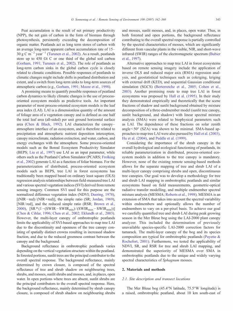
Fig. 3. False color composite (4, 3, 2 band combination) of the clipped subset ofthe Landsat TM scene of Mer Bleue, demonstrating the different spectralcharacteristics of the five considered land cover classes.

2.3. Multiple endmember spectral mixture analysis

Mixture decomposition with SMA is a widely appliedtechnique in passive optical remote sensing for determiningfractions of pixel components. SMA has been successfullyapplied in a wide range of disciplines including forestry (e.g.,Roberts et al., 2004), geology (e.g., Bryant, 1996), socialsciences (e.g., Schweik & Green, 1999), and urban studies (e.g.,Wu & Murray, 2003). In SMA it is assumed that the spectralreflectance of a pixel (ρλ′) is a mixture of the spectral reflectanceof individual scene components (endmembers), each weightedaccording to their abundance to produce the mixture. Further-more, it is typically assumed that the mixture is linear and thatmultiple scattering is negligible resulting in minimal interactionbetween scene elements (Adams et al., 1993; Hall et al., 1995;Roberts et al., 1993). The model is described by:

qk V¼XNi¼1

fi⁎qik þ ek ð3Þ

where ρiλ is the spectral reflectance of endmember i for aspecific band (λ), fi is the fraction of the endmember, N is thenumber of endmembers, and ελ is the residual error. A commonway to assess the fit of an endmember model is by the root meansquare error (RMSE), calculated as:

RMSE ¼

ffiffiffiffiffiffiffiffiffiffiffiffiffiffiffiffiffiffiXMk¼1

ðekÞ2

M

vuuuut ð4Þ

whereM is the number of bands. To produce accurate fractions,two constraints have to be imposed on the mixture decompo-sition. The first constraint requires that the fractions sum up toone and the second constraint requires the fractions to be non-negative (Heinz & Chang, 2001).

One of the most critical steps in the application of mixturedecomposition is the selection and proper spectral character-ization of suitable endmembers (Dennison & Roberts, 2003a;Tompkins et al., 1997). The spectral signature of endmemberscan be determined by spectroradiometer measurements in thefield or in the laboratory, selection of “pure” endmember pixelsfrom the image to be unmixed, or simulation with a radiativetransfer model. However, using a fixed set of endmembers, eachwith a single invariant spectral signature is a significantsimplification of the real world and a fundamental limitationof SMA since it might result in poor accuracy of fractions(Petrou & Foschi, 1999; Song, 2005; Theseira et al., 2003).Furthermore, SMA uses the same number of endmembers foreach pixel, not considering whether the respective endmemberis present in a pixel or not. To overcome these two limitations ofSMA, Roberts et al. (1998) introduced multiple endmemberspectral mixture analysis (MESMA) to account for the spectralvariability of endmembers and the varying number of end-members on a per-pixel basis. In MESMA, endmembers formixture decomposition are selected from a site-specific spectrallibrary containing the spectral signatures of suitable end-members. The endmember combination producing the lowestRMSE is assigned to each pixel (Roberts et al., 1998).

MESMA has been successfully applied in a wide range ofremote sensing studies including snow cover and area mapping(e.g., Painter et al., 2003), plant species mapping (e.g., Dennison& Roberts, 2003a,b; Roberts et al., 1998, 2003), soil mapping inarid lands (e.g., Okin et al., 2001), landform mapping (e.g.,Ballantine et al., 2005), fire temperature mapping (e.g.,Dennison et al., 2006), urban morphology (e.g., Rashed et al.,2003), and planetary mapping (e.g., Johnson et al., 2006; Li &Mustard, 2003).

Based on field observations, the spectral similarity amongtree and shrub canopies found in an exploratory study (datanot shown), and aerial photographs, it was determined that athree endmember model consisting of a general sunlit vascularplant canopy, sunlit Sphagnum moss, and shadow would be

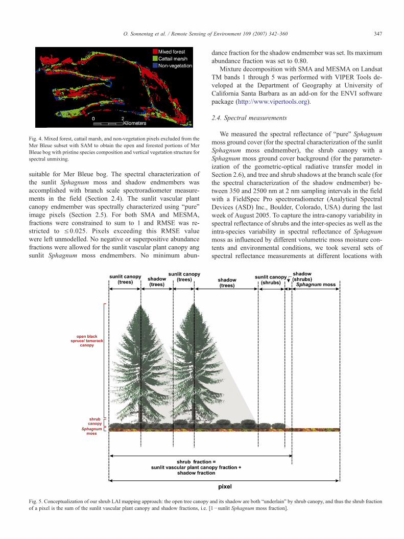
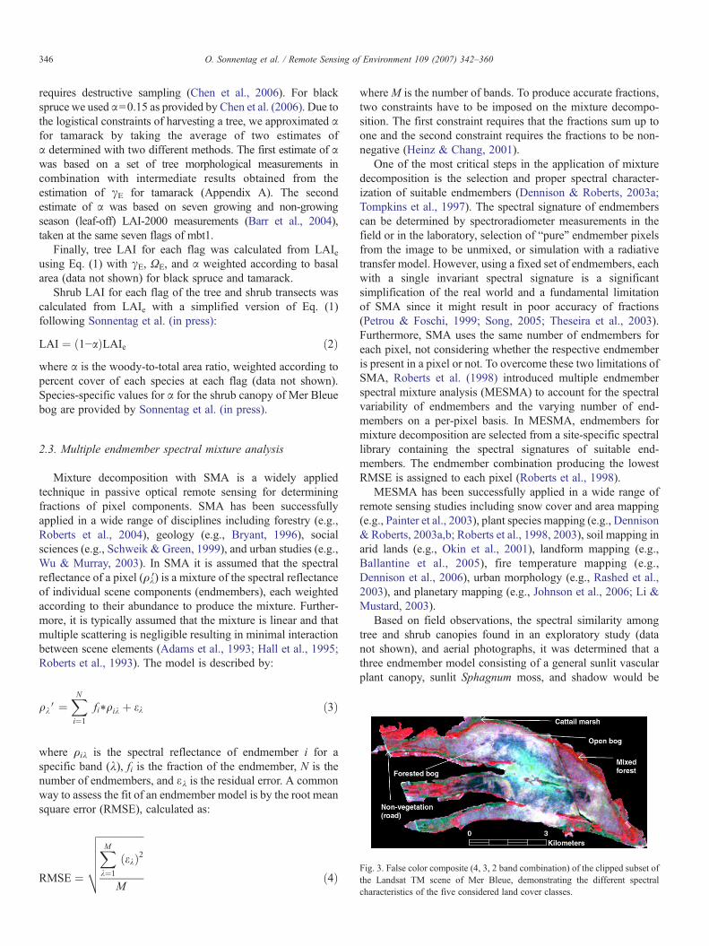
Fig. 4. Mixed forest, cattail marsh, and non-vegetation pixels excluded from theMer Bleue subset with SAM to obtain the open and forested portions of MerBleue bog with pristine species composition and vertical vegetation structure forspectral unmixing.


suitable for Mer Bleue bog. The spectral characterization ofthe sunlit Sphagnum moss and shadow endmembers wasaccomplished with branch scale spectroradiometer measure-ments in the field (Section 2.4). The sunlit vascular plantcanopy endmember was spectrally characterized using “pure”image pixels (Section 2.5). For both SMA and MESMA,fractions were constrained to sum to 1 and RMSE was re-stricted to ≤0.025. Pixels exceeding this RMSE valuewere left unmodelled. No negative or superpositive abundancefractions were allowed for the sunlit vascular plant canopy angsunlit Sphagnum moss endmembers. No minimum abun-

Fig. 5. Conceptualization of our shrub LAI mapping approach: the open tree canopy aof a pixel is the sum of the sunlit vascular plant canopy and shadow fractions, i.e. [

dance fraction for the shadow endmember was set. Its maximumabundance fraction was set to 0.80.

Mixture decomposition with SMA and MESMA on LandsatTM bands 1 through 5 was performed with VIPER Tools de-veloped at the Department of Geography at University ofCalifornia Santa Barbara as an add-on for the ENVI softwarepackage (http://www.vipertools.org).

2.4. Spectral measurements

We measured the spectral reflectance of “pure” Sphagnummoss ground cover (for the spectral characterization of the sunlitSphagnum moss endmember), the shrub canopy with aSphagnum moss ground cover background (for the parameter-ization of the geometric-optical radiative transfer model inSection 2.6), and tree and shrub shadows at the branch scale (forthe spectral characterization of the shadow endmember) be-tween 350 and 2500 nm at 2 nm sampling intervals in the fieldwith a FieldSpec Pro spectroradiometer (Analytical SpectralDevices (ASD) Inc., Boulder, Colorado, USA) during the lastweek of August 2005. To capture the intra-canopy variability inspectral reflectance of shrubs and the inter-species as well as theintra-species variability in spectral reflectance of Sphagnummoss as influenced by different volumetric moss moisture con-tents and environmental conditions, we took several sets ofspectral reflectance measurements at different locations with

nd its shadow are both “underlain” by shrub canopy, and thus the shrub fraction1− sunlit Sphagnum moss fraction].

http://www.vipertools.org


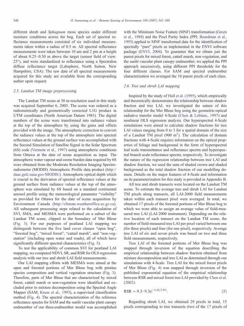
different shrub and Sphagnum moss species under differentmoisture conditions across the bog. Each set of spectral re-flectance measurements consisted of six individual measure-ments taken within a radius of 0.5 m. All spectral reflectancemeasurements were taken between 10 am and 2 pm at a heightof about 0.25–0.30 m above the target (sensor field of view:25°), and were standardized to reflectance using a Spectralondiffuse reflectance target (Labsphere, North Sutton, NewHampshire, USA). The raw data of all spectral measurementsacquired for this study are available from the correspondingauthor upon request.

2.5. Landsat TM image preprocessing

The Landsat TM scene at 30 m-resolution used in this studywas acquired September 6, 2005. The scene was ordered as aradiometrically and geometrically corrected L1G product inUTM coordinates (North American Datum 1983). The digitalnumbers of the scene were transformed into radiance valuesat the top of the atmosphere by using the gains and offsetsprovided with the image. The atmospheric correction to convertthe radiance values at the top of the atmosphere into spectralreflectance values at the ground surface was accomplished withthe Second Simulation of Satellite Signal in the Solar Spectrum(6S) code (Vermote et al., 1997) using atmospheric conditionsfrom Ottawa at the date of scene acquisition as input. Theatmospheric water vapour and ozone burden data required by 6Swere obtained from the Moderate Resolution Imaging Spectro-radiometer (MODIS) Atmospheric Profile data product (http://daac.gsfc.nasa.gov/MODIS/). Atmospheric optical depth whichis crucial in the derivation of spectral reflectance values at theground surface from radiance values at the top of the atmo-sphere was simulated by 6S based on a standard continentalaerosol profile using the meteorological parameter “visibility”as provided for Ottawa for the date of scene acquisition byEnvironment Canada (http://climate.weatheroffice.ec.gc.ca).All subsequent processing steps related to the calculation ofSVI, SMA, and MESMA were performed on a subset of theLandsat TM scene, clipped to the boundary of Mer Bleue(Fig. 3). For our purposes of peatland LAI mapping wedistinguish between the five land cover classes “open bog”,“forested bog”, “mixed forest”, “cattail marsh”, and “non-veg-etation” (including open water and roads), all of which havesignificantly different spectral characteristics (Fig. 3).

To test the applicability of common SVI for peatland LAImapping, we computed NDVI, SR, and RSR for OLS regressionanalysis with our tree and shrub LAI field measurements.

Our LAI mapping efforts with MESMA were aimed at theopen and forested portions of Mer Bleue bog with pristinespecies composition and vertical vegetation structure (Fig. 3).Therefore, parts of Mer Bleue that are characterized by mixedforest, cattail marsh or non-vegetation were identified and ex-cluded prior to mixture decomposition using the Spectral AngleMapper (SAM; Kruse et al., 1993), a supervised classificationmethod (Fig. 4). The spectral characterization of the referencereflectance spectra for SAM and the sunlit vascular plant canopyendmember of our three-endmember model was accomplished

with the Minimum Noise Feature (MNF) transformation (Greenet al., 1988) and the Pixel Purity Index (PPI; Boardman et al.,1995) applied to MNF transformed data for the identification ofspectrally “pure” pixels as implemented in the ENVI softwarepackage (ENVI, 2004). To guarantee that we obtain just thepurest pixels for mixed forest, cattail marsh, non-vegetation, andthe sunlit vascular plant canopy endmember, we applied the PPIapproach successively, using different PPI thresholds for thefour different classes. For SAM and spectral endmembercharacterization we averaged the 10 purest pixels of each class.

2.6. Tree and shrub LAI mapping

Inspired by the study of Hall et al. (1995), which empiricallyand theoretically demonstrates the relationship between shadowfraction and tree LAI, we investigated the nature of thisrelationship for the Mer Bleue bog using the geometric-opticalradiative transfer model 4-Scale (Chen & Leblanc, 1997) andnonlinear OLS regression analysis. Our hyperspectral 4-Scalesimulations were aimed to calculate shadow fractions for treeLAI values ranging from 0 to 3 for a spatial domain of the sizeof a Landsat TM pixel (900 m2). The calculation of domainfractions with 4-Scale requires information on the optical prop-erties of foliage and background in the form of hyperspectralleaf scale transmittance and reflectance spectra and hyperspec-tral branch scale reflectance spectra, respectively. To investigatethe nature of the regression relationship between tree LAI andshadow fraction, we used the sum of shaded crown and shadedbackground as the total shadow fraction of our modelling do-main. Details on the major features of 4-Scale and informationon its parameterization for this study is provided in Appendix B.

All tree and shrub transects were located on the Landsat TMscene. To estimate the average tree and shrub LAI for LandsatTM pixels along transects, all LAI-2000 field measurementstaken within each transect pixel were averaged. In total, weobtained 17 pixels of the forested portions of Mer Bleue bog towhich we were able to assign an average value of field-mea-sured tree LAI (LAI-2000 instrument). Depending on the rela-tive location of each transect on the Landsat TM scene, thenumber of field-measured tree LAI per pixel varied between one(for three pixels) and four (for one pixel), respectively. Averagetree LAI of six and seven pixels was based on two and threefield measurements, respectively.

Tree LAI of the forested portions of Mer Bleue bog wasmapped through inversion of the equation describing theempirical relationship between shadow fraction obtained frommixture decomposition and tree LAI as determined through oursimulations with 4-Scale. Tree LAI for the mixed forest pixelsof Mer Bleue (Fig. 4) was mapped through inversion of thepublished exponential equation of the empirical relationshipbetween RSR and mixed forest tree LAI provided by Chen et al.(2002):

RSR ¼ 9:3−9:3eð−LAI=2:93Þ: ð5Þ

Regarding shrub LAI, we obtained 29 pixels in total, 15pixels corresponding to tree transects (two of the 17 pixels of

http://daac.gsfc.nasa.gov/MODIS/

http://daac.gsfc.nasa.gov/MODIS/

http://climate.weatheroffice.ec.gc.ca

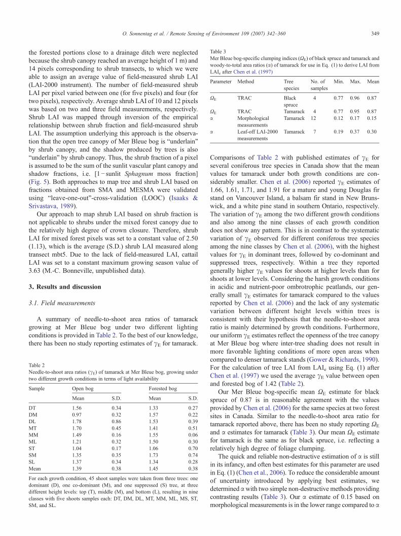
Table 3Mer Bleue bog-specific clumping indices (ΩE) of black spruce and tamarack andwoody-to-total area ratios (α) of tamarack for use in Eq. (1) to derive LAI fromLAIe after Chen et al. (1997)

Parameter Method Treespecies

No. ofsamples

Min. Max. Mean

ΩE TRAC Blackspruce

4 0.77 0.96 0.87

ΩE TRAC Tamarack 4 0.77 0.95 0.87α Morphological

measurementsTamarack 12 0.12 0.17 0.15

α Leaf-off LAI-2000measurements

Tamarack 7 0.19 0.37 0.30


the forested portions close to a drainage ditch were neglectedbecause the shrub canopy reached an average height of 1 m) and14 pixels corresponding to shrub transects, to which we wereable to assign an average value of field-measured shrub LAI(LAI-2000 instrument). The number of field-measured shrubLAI per pixel varied between one (for five pixels) and four (fortwo pixels), respectively. Average shrub LAI of 10 and 12 pixelswas based on two and three field measurements, respectively.Shrub LAI was mapped through inversion of the empiricalrelationship between shrub fraction and field-measured shrubLAI. The assumption underlying this approach is the observa-tion that the open tree canopy of Mer Bleue bog is “underlain”by shrub canopy, and the shadow produced by trees is also“underlain” by shrub canopy. Thus, the shrub fraction of a pixelis assumed to be the sum of the sunlit vascular plant canopy andshadow fractions, i.e. [1− sunlit Sphagnum moss fraction](Fig. 5). Both approaches to map tree and shrub LAI based onfractions obtained from SMA and MESMA were validatedusing “leave-one-out”-cross-validation (LOOC) (Isaaks &Srivastava, 1989).

Our approach to map shrub LAI based on shrub fraction isnot applicable to shrubs under the mixed forest canopy due tothe relatively high degree of crown closure. Therefore, shrubLAI for mixed forest pixels was set to a constant value of 2.50(1.13), which is the average (S.D.) shrub LAI measured alongtransect mbt5. Due to the lack of field-measured LAI, cattailLAI was set to a constant maximum growing season value of3.63 (M.-C. Bonneville, unpublished data).

3. Results and discussion

3.1. Field measurements

A summary of needle-to-shoot area ratios of tamarackgrowing at Mer Bleue bog under two different lightingconditions is provided in Table 2. To the best of our knowledge,there has been no study reporting estimates of γE for tamarack.

Table 2Needle-to-shoot area ratios (γE) of tamarack at Mer Bleue bog, growing undertwo different growth conditions in terms of light availability

Sample Open bog Forested bog

Mean S.D. Mean S.D.

DT 1.56 0.34 1.33 0.27DM 0.97 0.32 1.57 0.22DL 1.78 0.86 1.53 0.39MT 1.70 0.45 1.41 0.51MM 1.49 0.16 1.55 0.06ML 1.21 0.32 1.50 0.30ST 1.04 0.17 1.06 0.70SM 1.35 0.35 1.73 0.74SL 1.37 0.34 1.34 0.28Mean 1.39 0.38 1.45 0.38

For each growth condition, 45 shoot samples were taken from three trees: onedominant (D), one co-dominant (M), and one suppressed (S) tree, at threedifferent height levels: top (T), middle (M), and bottom (L), resulting in nineclasses with five shoots samples each: DT, DM, DL, MT, MM, ML, MS, ST,SM, and SL.

Comparisons of Table 2 with published estimates of γE forseveral coniferous tree species in Canada show that the meanvalues for tamarack under both growth conditions are con-siderably smaller. Chen et al. (2006) reported γE estimates of1.66, 1.61, 1.71, and 1.91 for a mature and young Douglas firstand on Vancouver Island, a balsam fir stand in New Bruns-wick, and a white pine stand in southern Ontario, respectively.The variation of γE among the two different growth conditionsand also among the nine classes of each growth conditiondoes not show any pattern. This is in contrast to the systematicvariation of γE observed for different coniferous tree speciesamong the nine classes by Chen et al. (2006), with the highestvalues for γE in dominant trees, followed by co-dominant andsuppressed trees, respectively. Within a tree they reportedgenerally higher γE values for shoots at higher levels than forshoots at lower levels. Considering the harsh growth conditionsin acidic and nutrient-poor ombrotrophic peatlands, our gen-erally small γE estimates for tamarack compared to the valuesreported by Chen et al. (2006) and the lack of any systematicvariation between different height levels within trees isconsistent with their hypothesis that the needle-to-shoot arearatio is mainly determined by growth conditions. Furthermore,our uniform γE estimates reflect the openness of the tree canopyat Mer Bleue bog where inter-tree shading does not result inmore favorable lighting conditions of more open areas whencompared to denser tamarack stands (Gower & Richards, 1990).For the calculation of tree LAI from LAIe using Eq. (1) afterChen et al. (1997) we used the average γE value between openand forested bog of 1.42 (Table 2).

Our Mer Bleue bog-specific mean ΩE estimate for blackspruce of 0.87 is in reasonable agreement with the valuesprovided by Chen et al. (2006) for the same species at two forestsites in Canada. Similar to the needle-to-shoot area ratio fortamarack reported above, there has been no study reporting ΩE

and α estimates for tamarack (Table 3). Our mean ΩE estimatefor tamarack is the same as for black spruce, i.e. reflecting arelatively high degree of foliage clumping.

The quick and reliable non-destructive estimation of α is stillin its infancy, and often best estimates for this parameter are usedin Eq. (1) (Chen et al., 2006). To reduce the considerable amountof uncertainty introduced by applying best estimates, wedetermined αwith two simple non-destructive methods providingcontrasting results (Table 3). Our α estimate of 0.15 based onmorphological measurements is in the lower range compared to α

Table 4Summary of field-measured tree and shrub LAI summarized according to therelative location of each transect on the subset of Landsat TM scene

Tree LAI[m2/m2]

Shrub LAI (forested bog)[m2/m2]

Shrub LAI (open bog)[m2/m2]

No. of pixels 17 15 14Min. LAI 0.23 0.76 0.73Max. LAI 3.06 2.87 3.05Mean LAI 1.59 1.57 1.50S.D. 0.83 0.61 0.67

Fig. 6. Mapped SVI for Mer Bleue computed from the atmospherically correctedLandsat TM subset: (A) NDVI, (B) SR, and (C) RSR.


estimates reported by Chen et al. (2006) for other coniferous treespecies in Canada, whereas an α estimate of 0.30 is in the higherrange. We assume that the α estimate based on morphologicalmeasurements is underestimated due to the nature of the approachof simply using mean values of a few morphological measure-ments. Our α estimate based on leaf-off LAI-2000 measurementsis most likely overestimated due to the timing of the non-growingseason LAI-2000 measurement at dusk after a sunny day in mid-November. The short sunset provided us just with a very shorttime window with diffuse light conditions to take the measure-ments. The highest individual α values coincide with the lastmeasurements when it was probably too dark, resulting in anoverestimation of non-growing season LAIe and thus α. Weassume that our two contrasting α estimates define the limits of itsactual mean value, and thus we used the average of both estimatesof 0.225 for application in Eq. (1).

The final averaged tree and shrub LAI values per pixel aftercorrecting LAIe for γE, ΩE, and α (tree LAI) and for α (shrubLAI) with Eqs. (1) and (2), respectively, are provided in Table 4.Tree LAI varies over a wide range from 0.23 and 3.06, resultingin a mean value of 1.59. This average tree LAI is much smallerthan the average tree LAI of several forest sites in Canada (Chenet al., 2006), and thus reflects the low productivity of acidic andnutrient-poor ombrotrophic peatlands. Shrub LAI varies over arange similar to tree LAI, with a slightly lower mean shrub LAImeasured along transects located in open areas of the bogcompared to forested portions. The similar ranges and means oftree and shrub LAI, respectively, provided by Table 4 indicatethe importance of the shrub canopy in the Mer Bleue bog'shydrological and ecological functioning as described in severalstudies (e.g., Lafleur et al., 2005; Moore et al., 2002).

3.2. Spectral vegetation indices for Mer Bleue

All three SVI computed from the atmospherically correctedLandsat TM subset of Fig. 3 respond to the dense tree canopyalong drainage ditches and the beaver ponds with the highestvalues for Mer Bleue (Fig. 6). Non-vegetation pixels yield thelowest values for the respective SVI (e.g., the southern beaverpond of the northern finger delineating Mer Bleue bog,portions of the drainage dissecting the eastern half of MerBleue bog). Intermediate between these two extremes are thecattail marshes and areas of Mer Bleue bog characterized bypristine species composition and vertical vegetation structure.The central part of Mer Bleue bog, in particular, responds withvalues for the respective SVI similar to non-vegetation pixels,

thus indicating sparse vascular vegetation. However, fromfield observations and aerial photographs (data not shown) weknow that these central areas comprise very open patches oftypical black spruce and tamarack canopies over an alsorelatively open and low shrub canopy. Thus, in these areas, themajor contributor to background reflectance is the Sphagnummoss ground cover, with spectral features that do not allow forthe adequate characterization of the absorption in the redportion of the visible range and the high reflectance of theNIR range of the vascular plants (Fig. 8).

The linear OLS regression relationships between the SVIof Fig. 6 and the field-measured tree and shrub LAI (openbog) of Table 4 are provided by Fig. 7. Regarding tree LAI,the highest value for R2 is obtained for RSR (R2 =0.27),followed by SR (R2 =0.13) and NDVI (R2 =0.09), respective-ly. Generally, the R2 values for the Mer Bleue bog aresignificantly smaller than those obtained in boreal forestecosystems (e.g., Brown et al., 2000; Chen et al., 2002),indicating for each pixel that there is no single SVI vs. treeLAI linear regression relationship but a set of relationships, allof which are a function of crown closure and thus of the nature

Fig. 7. Linear OLS regression relationships between SVI (Fig. 6) and field-measured tree and shrub LAI: A) NDVI vs. tree LAI, B) NDVI vs. shrub LAI, C) SR vs. treeLAI, D) SR vs. shrub LAI, E) RSR vs. tree LAI, and F) RSR vs. tree LAI.


of background reflectance. However, the general superiority ofRSR over SR and NDVI for tree LAI mapping in borealforests due to its capability to compensate for differences incanopy closure and background reflectance was demonstratedin several previous studies (e.g., Brown et al., 2000; Chenet al., 2002). For shrub LAI, the highest value for R2 is againobtained for RSR (R2 =0.71), followed by SR (R2 =0.70) andNDVI (R2 =0.64), respectively. These significantly higher R2

values for all three SVI demonstrate their general applicability

Fig. 8. Sphagnum moss reflectance spectra measured at Mer Bleue bog: nineindividual sample sets for mixture decomposition with MESMA, and theiraverage (bold line) for mixture decomposition with SMA.

to the shrub canopy of the open portions of the Mer Bleuebog. However, none of the SVI of Fig. 7 allows for mappingof shrub LAI of the forested portions of Mer Bleue bog.

3.3. Mixture decomposition with SMA and MESMA

We used nine Sphagnum moss reflectance spectra measuredat Mer Bleue bog convolved to the wavelength rangecorresponding to the Landsat TM bands 1 through 5 for mixture

Fig. 9. Spectral characterization of the three-endmember model for mixturedecomposition with SMA (convolved to the mid-points of the Landsat bands 1through 5): sunlit vascular plant canopy, sunlit Sphagnum moss, and shadow.


decomposition (Fig. 8). All nine reflectance spectra are char-acterized by diagnostic reflectance differences in the visible,NIR, and SWIR distinguishing them from the reflectance spec-tra of vascular plants. Generally, Sphagnum moss is more re-flective in the red portion of the visible range and less reflectivein the NIR range than vascular plants. Further characteristicfeatures of Sphagnum moss reflectance spectra described byBubier et al. (1997) are the strong water absorption features atabout 980 and 1200 nm, resulting in three distinctive spectralreflectance peaks at about 930, 1100, and 1300 nm (Fig. 8).

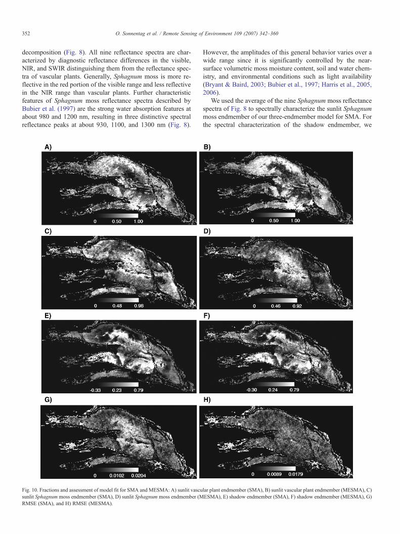
Fig. 10. Fractions and assessment of model fit for SMA and MESMA: A) sunlit vascusunlit Sphagnum moss endmember (SMA), D) sunlit Sphagnum moss endmember (MRMSE (SMA), and H) RMSE (MESMA).

However, the amplitudes of this general behavior varies over awide range since it is significantly controlled by the near-surface volumetric moss moisture content, soil and water chem-istry, and environmental conditions such as light availability(Bryant & Baird, 2003; Bubier et al., 1997; Harris et al., 2005,2006).

We used the average of the nine Sphagnum moss reflectancespectra of Fig. 8 to spectrally characterize the sunlit Sphagnummoss endmember of our three-endmember model for SMA. Forthe spectral characterization of the shadow endmember, we

lar plant endmember (SMA), B) sunlit vascular plant endmember (MESMA), C)ESMA), E) shadow endmember (SMA), F) shadow endmember (MESMA), G)

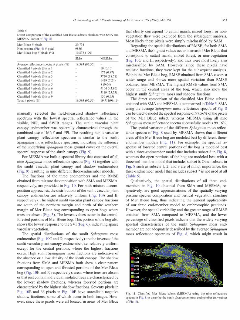
Table 5Direct comparison of the classified Mer Bleue subsets obtained with SMA andMESMA (subset of Fig. 8)

Mer Bleue # pixels 29,734Non-pristine (Fig. 4) # pixel 9856Mer Bleue bog # pixels (%) 19,878 (100)

SMA MESMA

Average reflectance spectra # pixels (%) 19,393 (97.56) –Classified # pixels (%) ss 1 – 19 (0.10)Classified # pixels (%) ss 2 – 172 (0.87)Classified # pixels (%) ss 3 – 3720 (18.71)Classified # pixels (%) ss 4 – 1439 (7.24)Classified # pixels (%) ss 5 – 8 (0.04)Classified # pixels (%) ss 6 – 9104 (45.80)Classified # pixels (%) ss 8 – 5119 (25.75)Classified # pixels (%) ss 9 – 130 (0.65)Total # pixels (%) 19,393 (97.56) 19,711(99.16)

Fig. 11. Classified Mer Bleue subset (MESMA) using the nine reflectancespectra in Fig. 8 to describe the sunlit Sphagnum moss endmember (ss=subsetof Fig. 8).


manually selected the field-measured shadow reflectancespectrum with the lowest spectral reflectance values in thevisible, NIR, and SWIR ranges. The sunlit vascular plantcanopy endmember was spectrally characterized through thecombined use of MNF and PPI. The resulting sunlit vascularplant canopy reflectance spectrum is similar to the sunlitSphagnum moss reflectance spectrum, indicating the influenceof the underlying Sphagnum moss ground cover on the overallspectral response of the shrub canopy (Fig. 9).

For MESMA we built a spectral library that consisted of allnine Sphagnum moss reflectance spectra (Fig. 8) together withthe sunlit vascular plant canopy and shadow endmembers(Fig. 9) resulting in nine different three-endmember models.

The fractions of the three endmembers and the RMSEobtained from mixture decomposition with SMA and MESMA,respectively, are provided in Fig. 10. For both mixture decom-position approaches, the distributions of the sunlit vascular plantcanopy endmember are relatively uniform (Fig. 10A and B,respectively). The highest sunlit vascular plant canopy fractionsare south of the northern margin and north of the southernmargin of Mer Bleue bog corresponding to open bogs wheretrees are absent (Fig. 3). The lowest values occur in the central,forested portions of Mer Bleue bog. This portion of the bog alsoshows the lowest response to the SVI (Fig. 6), indicating sparsevascular vegetation.

The spatial distributions of the sunlit Sphagnum mossendmember (Fig. 10C and D, respectively) are the inverse of thesunlit vascular plant canopy endmember, i.e. relatively uniformexcept for the central portions, where the highest fractionsoccur. High sunlit Sphagnum moss fractions are indicative ofthe absence or a low density of the shrub canopy. The shadowfractions from SMA and MESMA both show a clear patterncorresponding to open and forested portions of the Mer Bleuebog (Fig. 10E and F, respectively): areas where trees are absentor that just contain individual, isolated trees are characterized bythe lowest shadow fractions, whereas forested portions arecharacterized by the highest shadow fractions. Seventy pixels inFig. 10E and 66 pixels in Fig. 10F have unrealistic negativeshadow fractions, some of which occur in both images. How-ever, since these pixels were all located in areas of Mer Bleue

that clearly correspond to cattail marsh, mixed forest, or non-vegetation they were excluded from the subsequent analysis.Most likely these pixels were simply misclassified by SAM.

Regarding the spatial distributions of RMSE, for both SMAandMESMA the highest values occur in areas of Mer Bleue thatcorrespond to cattail marsh, mixed forest, or non-vegetation(Fig. 10G and H, respectively), and thus were most likely alsomisclassified by SAM. However, since these pixels haverealistic fractions, they were kept for the subsequent analysis.Within the Mer Bleue bog, RMSE obtained from SMA covers awider range and shows more spatial variation than RMSEobtained from MESMA. The highest RMSE values from SMAoccur in the central areas of the bog, which also show thehighest sunlit Sphagnum moss and shadow fractions.

The direct comparison of the classified Mer Bleue subsetsobtained with SMA andMESMA is summarized in Table 5. SMAusing the average Sphagnum moss reflectance spectra of Fig. 8can be used to model the spectral response of 97.56% of the pixelsof the Mer Bleue subset, whereas MESMA using all nineSphagnum moss reflectance spectra successfully models 99.16%.

The spatial variation of the different Sphagnum moss reflec-tance spectra of Fig. 8 used by MESMA shows that differentareas of the Mer Bleue bog are modeled best by different three-endmember models (Fig. 11). For example, the spectral re-sponse of forested central portions of the bog is modeled bestwith a three-endmember model that includes subset 8 in Fig. 8,whereas the open portions of the bog are modeled best with athree end-member model that includes subset 6. Other subsets inFig. 8 such as subsets 1, 2, and 9 are of minor importance, thethree-endmember model that includes subset 7 is not used at all(Table 5).

Qualitatively, the spatial distributions of all three end-members in Fig. 10 obtained from SMA and MESMA, re-spectively, are good approximations of the spatially varyingpristine species composition and vertical vegetation structureof Mer Bleue bog, thus indicating the general applicabilityof our three end-member model to ombrotrophic peatlands.However, the spatial variability and the greater range of RMSEobtained from SMA compared to MESMA, and the lowerpercentage of classified pixels indicate that the widely varyingspectral characteristics of the sunlit Sphagnum moss end-member are not adequately described by the average Sphagnummoss reflectance spectrum of Fig. 8, which might result in


less accurate fractions. Furthermore, by using a range of dif-ferent Sphagnum moss reflectance spectra, the influence of thesimilarity between the average sunlit Sphagnum moss and thesunlit vascular plant canopy reflectance spectra is minimized(Fig. 9). Less accurate fractions limit the use of SMA forpeatland LAI mapping as demonstrated in Section 3.5.

3.4. Geometric-optical radiative transfer modeling

The simulated relationship between shadow fraction and treeLAI is clearly not linear but appears to be of exponential natureand is best described with a nonlinear exponential equation ofthe general form (Fig. 12):

y ¼ a−b⁎expð−x=cÞ ð6Þwhere x and y are tree LAI and shadow fractions, respectively,and a, b, and c are regression constants. The constants a, b, andc of Eq. (6) describe the simulated exponential relationshipbetween tree LAI and shadow fraction and were determinedthrough unconstrained, non-linear OLS regression analysis as0.361, 0.326, and 1.698, respectively (Fig. 12).

The first constant in Eq. (6), a, is the maximum shadowfraction, and the second constant, b, is the difference betweenmaximum shadow fraction and background shadow, i.e. shadowproduced by the shrub canopy, since no trees are present at a treeLAI value of zero. Thus, for our simulated relationship theamount of shadow produced by the shrub canopy is estimated as0.035.

3.5. Tree and shrub LAI mapping using MESMA

Based on Eq. (6) we determined the regression relationshipsbetween tree LAI (Table 4) and shadow fractions obtained fromSMA (Fig. 10E) and MESMA (Fig. 10F), respectively, throughpartially constrained non-linear OLS regression analysis(Fig. 13A and B, respectively). In both the regression relation-ships of Fig. 13A and B the first regression constant, a, was

Fig. 12. Simulated exponential relationship between shadow fraction (SF) andtree LAI for a Landsat TM pixel of Mer Bleue bog.

preset to the maximum shadow fraction obtained from mixturedecomposition (Fig. 10E and F, respectively). The second re-gression constant, b, was pre-set to the difference of the firstregression constant and background shadow. An average back-ground shadow of 0.09 produced by the shrub canopy wascalculated based on pixels corresponding to the three shrubtransects mbs1, mbs2, and mbs3 located in open areas of theMerBleue bog where trees were absent. The third regression con-stant, c, was determined iteratively through the regression anal-ysis. Comparison of the R2 values obtained through the mixturedecomposition-based non-linear OLS regression (Fig. 13A andB, respectively) with those from the SVI-based linear OLSregression (Fig. 7A, C, and E, respectively) reveals that theshadow fraction is generally a strong predictor of tree LAI inombrotrophic peatlands, with MESMA being superior overSMA as indicated by R2 values of 0.75 (Fig. 13B) and 0.61(Fig. 13A), respectively. Similar findings demonstrating thegeneral superiority of the shadow fraction over SVI for tree LAIestimation were made by Hall et al. (1995) and Hall et al. (2003).

For the estimation of shrub LAI based on shrub fraction wealso applied the approach of partially constrained non-linearOLS regression analysis using Eq. (6) (Fig. 13C and D, re-spectively). A simple plot of field-measured shrub LAI and theshrub fractions obtained from SMA and MESMA revealed thatthe shrub fraction reaches a plateau at about 0.90 despiteincreasing shrub LAI. A possible reason for this might be thatincreasing shrub LAI is inherent with increasing shrub fractionup to a certain point, after which shrub LAI increases as afunction of shrub height resulting in more foliage seen by theLAI-2000 instrument sensor but not necessarily in a higherfraction of shrubs covering the ground as determined throughSMA and MESMA, respectively. This interpretation is sup-ported by the observation that the highest shrub LAI valuesalong our transects were measured at mbt5 and mbs3, both ofwhich are close to a drainage ditch and to the margin of MerBleue bog, respectively. Both areas are characterized by lowerwater table positions with more favorable growth conditions,resulting in higher and denser shrub canopies. In both OLSregression relationships of Fig. 13C and D, respectively, the firstregression constant, a, was pre-set to a maximum shrub fractionof 0.90, representing the plateau of the exponential relationship.The background was set to zero, since if shrubs are absent,shrub LAI is supposed to equal zero. Our simple approach ofcalculating the shrub fraction as the sum of the sunlit vascularplant canopy and the shadow fraction (i.e. [1− sunlit Sphagnummoss fraction]) most likely resulted in overestimation of theshrub fraction for some areas of Mer Bleue bog since it does notaccount for the situation where shadows produced by trees are“underlain” directly by Sphagnum moss, i.e. where the shrubcanopy is absent. However, we assume that this overestimationis on average balanced by the underestimation that would resultfrom the correction of 0.09 to the shadow fraction for theaverage shadow produced by the shrub canopy estimated above.Simple comparison of the R2 values obtained through the mix-ture decomposition-based non-linear OLS regression (Fig. 13Cand D, respectively) with those from the SVI-based linear OLSregression (Fig. 7B, D, and F, respectively) might suggest that

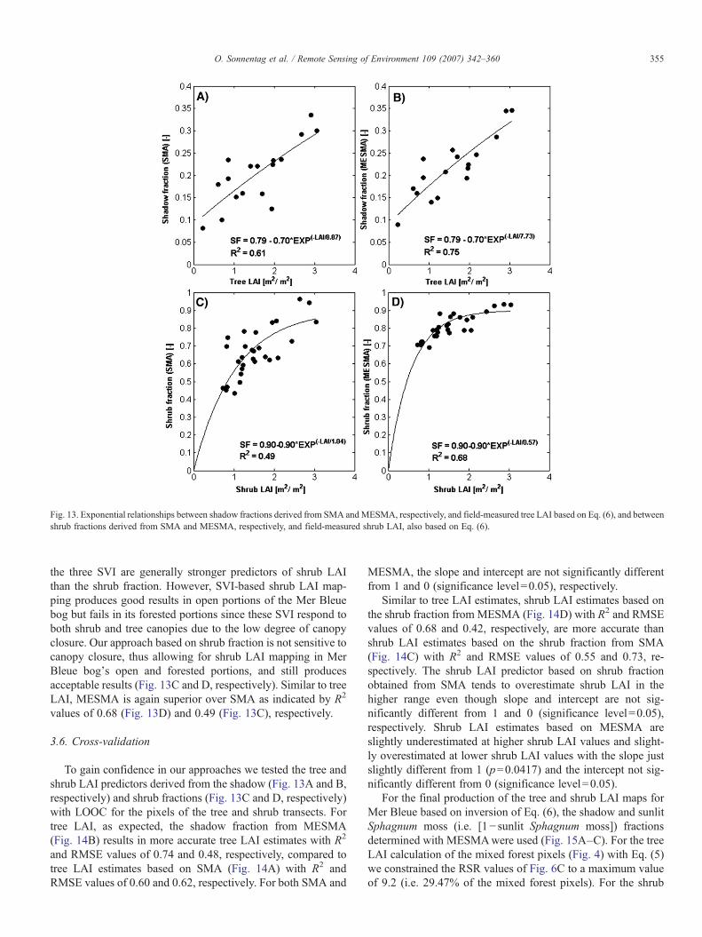
Fig. 13. Exponential relationships between shadow fractions derived from SMA andMESMA, respectively, and field-measured tree LAI based on Eq. (6), and betweenshrub fractions derived from SMA and MESMA, respectively, and field-measured shrub LAI, also based on Eq. (6).


the three SVI are generally stronger predictors of shrub LAIthan the shrub fraction. However, SVI-based shrub LAI map-ping produces good results in open portions of the Mer Bleuebog but fails in its forested portions since these SVI respond toboth shrub and tree canopies due to the low degree of canopyclosure. Our approach based on shrub fraction is not sensitive tocanopy closure, thus allowing for shrub LAI mapping in MerBleue bog's open and forested portions, and still producesacceptable results (Fig. 13C and D, respectively). Similar to treeLAI, MESMA is again superior over SMA as indicated by R2

values of 0.68 (Fig. 13D) and 0.49 (Fig. 13C), respectively.

3.6. Cross-validation

To gain confidence in our approaches we tested the tree andshrub LAI predictors derived from the shadow (Fig. 13A and B,respectively) and shrub fractions (Fig. 13C and D, respectively)with LOOC for the pixels of the tree and shrub transects. Fortree LAI, as expected, the shadow fraction from MESMA(Fig. 14B) results in more accurate tree LAI estimates with R2

and RMSE values of 0.74 and 0.48, respectively, compared totree LAI estimates based on SMA (Fig. 14A) with R2 andRMSE values of 0.60 and 0.62, respectively. For both SMA and

MESMA, the slope and intercept are not significantly differentfrom 1 and 0 (significance level=0.05), respectively.

Similar to tree LAI estimates, shrub LAI estimates based onthe shrub fraction from MESMA (Fig. 14D) with R2 and RMSEvalues of 0.68 and 0.42, respectively, are more accurate thanshrub LAI estimates based on the shrub fraction from SMA(Fig. 14C) with R2 and RMSE values of 0.55 and 0.73, re-spectively. The shrub LAI predictor based on shrub fractionobtained from SMA tends to overestimate shrub LAI in thehigher range even though slope and intercept are not sig-nificantly different from 1 and 0 (significance level=0.05),respectively. Shrub LAI estimates based on MESMA areslightly underestimated at higher shrub LAI values and slight-ly overestimated at lower shrub LAI values with the slope justslightly different from 1 (p=0.0417) and the intercept not sig-nificantly different from 0 (significance level=0.05).

For the final production of the tree and shrub LAI maps forMer Bleue based on inversion of Eq. (6), the shadow and sunlitSphagnum moss (i.e. [1− sunlit Sphagnum moss]) fractionsdetermined with MESMAwere used (Fig. 15A–C). For the treeLAI calculation of the mixed forest pixels (Fig. 4) with Eq. (5)we constrained the RSR values of Fig. 6C to a maximum valueof 9.2 (i.e. 29.47% of the mixed forest pixels). For the shrub

Fig. 14. “Leave-one-out”-cross-validation (LOOC) for tree LAI estimated based on shadow fraction obtained from SMA (A) and MESMA (B), and for shrub LAIestimated based on shrub fraction obtained from SMA (C) and MESMA (D).


LAI calculation with Eq. (6) based on Fig. 10F, we constrainedthe shrub fraction of a pixel to a maximum value of 0.89 (i.e.9.34% of Mer Bleue bog). We consider this constraint to bereasonable since at Mer Bleue bog a shrub fraction greater than0.90 over an area of 900 m2 is unrealistic due to the bog'smicrotopography. On average, hollows, which make up approx-imately one third of Mer Bleue bog's surface area (Lafleur et al.,2005), have a percent cover of less than 0.5, and thus full shrubcoverage over large areas does not exist (Sonnentag et al.,in press).

Total LAI was calculated as the sum of tree and shrub LAI(Fig. 15C). In all three maps, non-vegetation pixels (Fig. 4),pixels that were excluded due to negative shadow fractions(Fig. 10F), and unclassified pixels (Fig. 11) were set to NoData.Qualitatively, the LAI maps of Fig. 15 capture the spatialvariation of the species composition and vertical vegetationstructure of Mer Bleue quite well when compared to Fig. 3. Asexpected, the highest total LAI values occur along beaver pondsand drainage ditches, whereas the Mer Bleue bog is character-ized by considerably lower total LAI values. A striking featureof the shrub LAI map is the generally low shrub LAI values inthe central forested parts of Mer Bleue bog as indicated by thefractions of Fig. 10 (Fig. 15B). The SVI of Fig. 6 indicate sparsevascular vegetation for these portions of the Mer Bleue bog,which would result in low total LAI values. However, the totalLAI of these areas is in the same range as for the open portions

of Mer Bleue bog, with the tree LAI as the major contributor tototal LAI.

4. Conclusions

Tree LAI of forest ecosystem has routinely been mappedbased on the empirical relationships between SVI derived fromremote sensing imagery and LAI field measurements. Thesuitability of this approach is limited for tree and shrub LAImapping in ombrotrophic peatlands, mainly due to the spatiallyvarying vegetation structure of their multi-layer canopy, whichusually includes a moss ground cover. Additionally, mosseshave spectral characteristics that are significantly different fromvascular plants.

Based on a promising approach to map tree LAI in forestecosystems using fractions from mixture decomposition withSMA, we mapped tree and shrub LAI of an ombrotrophicpeatland at the peak growing season. Applying MESMA, anextension of SMA, to a three-endmember model comprising ageneral sunlit vascular plant canopy, Sphagnum moss, andshadow, the widely varying spectral characteristics of Sphag-num mosses were taken into account in the mixture decompo-sition. A slightly higher percentage of pixels of the Mer Bleuebog were successfully unmixed by our three endmember modelwith MESMA than with SMA. Furthermore, mixture decom-position with MESMA reduces the RMSE, mainly in portions

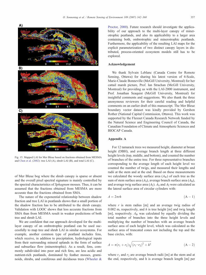
Fig. 15. Mapped LAI for Mer Bleue based on fractions obtained from MESMAand Chen et al. (2002): tree LAI (A), shrub LAI (B), and total LAI (C).


of Mer Bleue bog where the shrub canopy is sparse or absentand the overall pixel spectral signature is mainly controlled bythe spectral characteristics of Sphagnum mosses. Thus, it can beassumed that the fractions obtained from MESMA are moreaccurate than the fractions obtained from SMA.

The nature of the exponential relationship between shadowfraction and tree LAI in peatlands shows that a small portion ofthe shadow fraction has to be attributed to the shrub canopy.Validation with LOOC shows that less accurate fractions fromSMA than from MESMA result in weaker predictions of bothtree and shrub LAI.

We are confident that our approach developed for the multi-layer canopy of an ombrotrophic peatland can be used suc-cessfully to map tree and shrub LAI in similar ecosystems. Forexample, another common type of peatland includes fens,which receive, in addition to precipitation, hydrological inputsfrom their surrounding mineral uplands in the form of surfaceand subsurface flow (minerotrophic). As a result, fens, com-monly subdivided into poor and rich fens, are less acidic andnutrient-rich peatlands, dominated by feather mosses, grami-noids, shrubs, and coniferous and deciduous trees (Wheeler &

Proctor, 2000). Future research should investigate the applica-bility of our approach to the multi-layer canopy of miner-otrophic peatlands, and also its applicability to a larger areacontaining both, ombrotrophic and minerotrophic peatlands.Furthermore, the applicability of the resulting LAI maps for theexplicit parameterization of two distinct canopy layers in dis-tributed, process-oriented ecosystem models still has to beexplored.

Acknowledgement

We thank Sylvain Leblanc (Canada Centre for RemoteSensing, Ottawa) for sharing his latest version of 4-Scale,Marie-Claude Bonneville (McGill University, Montreal) for hercattail marsh picture, Prof. Ian Strachan (McGill University,Montreal) for providing us with the LAI-2000 instrument, andProf. Jonathan Seaquist (McGill University, Montreal) forinsightful comments and suggestions. We also thank the threeanonymous reviewers for their careful reading and helpfulcomments on an earlier draft of this manuscript. The Mer Bleueboundary vector dataset was kindly provided by GershonRother (National Capital Commission, Ottawa). This work wassupported by the Fluxnet Canada Research Network funded bythe Natural Science and Engineering Council of Canada, theCanadian Foundation of Climate and Atmospheric Sciences andBIOCAP Canada.

Appendix A

For 12 tamarack trees we measured height, diameter at breastheight (DBH), and average branch length at three differentheight levels (top, middle, and bottom), and counted the numberof branches of the entire tree. For three representative branchescorresponding to the average length of each height level wecounted the number of twigs, and measured their lengths andradii at the stem and at the end. Based on these measurementswe calculated the woody surface area (AW) of each tree as thesum of stem surface area (AS), average branch surface area (AB),and average twig surface area (AT). AS and ATwere calculated asthe lateral surface area of circular cylinders with:

A ¼ 2prh ðA� 1Þ

where r is stem radius [m] and an average twig radius of0.002 m, respectively, and h is tree height [m] and twig length[m], respectively. AB was calculated by equally dividing thetotal number of branches into the three height levels andmultiplying the number of branches with an average branchsurface area of each height level, which was calculated as thesurface area of truncated cones not including the top and thebase circles, with:

A ¼ pðr1 þ r2Þffiffiffiffiffiffiffiffiffiffiffiffiffiffiffiffiffiffiffiffiffiffiffiffiffiffiffiðr1−r2Þ2 þ h2

qðA� 2Þ

where r1 and r2 are average branch radii [m] at the stem and atthe end, respectively, and h is average branch length [m] per


height level of each tree. The calculation of total tree leaf area(AL) is based on a needle-to-woody area ratio ε, which wecalculated based on the 90 tamarack shoot samples collected forthe needle-to-shoot area estimation with:

e ¼P

ANPAT

ðA� 3Þ

where AN is half the total needle area (including all sides) in ashoot [m2], and AT is half the total woody area [m2] of a shootsample, i.e. half the surface area of its twig. AT was calculatedusing Eq. (A-1) with the average twig radius of 0.002 mdetermined as part of the previous tree woody area calculation,and the twig length [m] of the respective shoot sample. Basedon Eq. (A-3) we calculated an average value for ε of 11.69. Thetotal needle surface area of each tree was calculated as the sumof the top, middle, and bottom level needle surface areas, whichin turn were calculated by multiplying ε with the twig surfacearea of the respective height level as determined in the previoustree woody area calculation. Using AWand AN, we calculated anaverage value for α in accordance with Kucharik et al. (1998)with:

a ¼P

AWPAW þP

ANðA� 4Þ

Appendix B

The geometric-optical radiative transfer model 4-Scaleconsiders the interaction of light with architectural elementsof tree canopies at four different scales: tree groups, tree crowns,branches, and foliage elements. To simulate the patchinessusually observed in boreal forests, 4-Scale uses a Neyman typeA distribution, assuming that trees are combined in groups, withthe center of the group entirely contained in quadrats that dividethe simulation domain into smaller areas (Chen & Leblanc,1997). A geometry-based multiple scattering scheme considersthe scattering of light between all architectural canopy elements(Chen & Leblanc, 2001).

In our study we parameterized 4-Scale using averaged leafscale western larch (Larix occidentalis) reflectance and trans-mittance spectra obtained as part of a previous study (D.A.Roberts, unpublished data). The leaf scale spectra were mea-sured using a modified Beckman DK2A with an integratingsphere attachment designed for measurements of directionalhemispherical transmittance or reflectance. Western larch spec-tra were collected from needles destructively sampled from thesunlit portions of lower tree crowns. After collection, needleswere stored cooled and transported to the laboratory for spectralmeasurements. Spectra were collected within 48 h of originalcollection. Laboratory spectra were collected from needles ar-ranged on slide mounts with minimal gaps and overlaps asdescribed by Roberts et al. (2004). Regarding the optical prop-erties of background, we parameterized 4-Scale using the avera-ge of nine sets of branch scale background reflectance spectraobtained in this study.

In addition to leaf and branch scale input reflectancespectra, 4-Scale requires several site- and tree architecturespecific input parameters including tree LAI and stand density.To avoid the arbitrary variation of stand density withincreasing tree LAI or the “growth” of bigger trees with lessfoliage by keeping stand density constant with increasing treeLAI, we determined the empirical relationship between standdensity and tree LAI with unconstrained nonlinear OLSregression analysis for a total of nine flags of mbt3, mbt4,and mbt5.

Based on the exponential stand density vs. tree LAIrelationship (R2 = 0.62) we estimated stand densitiescorresponding to tree LAI values of 0.1, 0.5, 1.0, 1.5, 2.0,2.5, and 3.0 (Table B-1). For comparison of simulated shadowfractions with shadow fractions derived from the subset of theLandsat TM scene with SMA and MESMA, the simulationswere performed using a SZA corresponding to date and time ofimage acquisition and a viewing zenith angle (VZA) of 0°.Other parameters required by 4-Scale are based on fieldobservations (stick and crown height, crown radius, andfoliage element size) and measurements (clumping index,needle-to-shoot area ratio) obtained in this study, or are setfollowing literature recommendations (number of quadrats,Neyman A grouping, and repulsion factor that avoidsunnatural tree crown overlapping) after Chen and Leblanc(1997).

Based on the input spectra and the site- and tree architecturespecific input parameters of Table B-1, 4-Scale calculates thespectral reflectance of the four domain components sunlit andshaded crown, and sunlit and shaded background, together withtheir respective fractions. The overall domain spectral reflec-tance is calculated by associating the spectral reflectance of thedomain components with their fractions according to Eq. (3)without the residual error.

Table B-1: 4-Scale parameterizations used to investigate thenature of the empirical relationship between shadow fractionand tree LAI for Mer Bleue bog

LAI
0.1 0.5 1 1.5 2 2.5 3
Siteparameters

Size
900 900 900 900 900 900 900 Standdensity[trees/900 m2]
64
64 153 294 354 380 391
Treeclumping

# Quadrats [-]
5 5 5 5 5 5 5 Neyman Agrouping [-]
2
2 2 2 2 2 2
Other
SZA [°] 43 43 43 43 43 43 43 VZA [°] 0 0 0 0 0 0 0 Stick height [m] 0.2 0.2 0.2 0.1 0.1 0.1 0.1 Crown height [m] 1.7 1.7 1.7 1.1 1.1 1.1 1.1 Crown radius [m] 0.7 0.4 0.4 0.3 0.3 0.3 0.3 Clumping index [-] 0.87 0.87 0.87 0.87 0.87 0.87 0.87 Apex angle [°] 13 13 13 13 13 13 13 Needle-to-shootarea ratio [-]
1.41
1.41 1.41 1.41 1.41 1.41 1.41
Foliageelementsize [m]

0.05
0.05 0.05 0.05 0.05 0.05 0.05
Repulsionfactor

0.5
0.5 0.5 0.5 0.5 0.5 0.5


References

Adams, J. N., Smith, M. O., & Gillespie, A. R. (1993). Imaging spectrometry:Interpretation based on spectral mixture analysis. In C. M. Pieters, & P. A. J.Englert (Eds.), Remote geochemical analysis: Elemental and mineralogicalcomposition (pp. 145−166). Cambridge, England: Press Syndicate ofUniversity of Cambridge.

Baldocchi, D., Kelliher, F. M., Black, T. A., & Jarvis, P. G. (2000). Climate andvegetation controls on boreal zone energy exchange. Global Change Biology,6, 69−83.

Ballantine, J. -A. C., Okin, G. S., Prentiss, D. E., & Roberts, D. A. (2005).Mapping African landforms using continental scale unmixing of MODISimagery. Remote Sensing of Environment, 97, 470−483.

Barr, A. G., Black, T. A., Hogg, E. H., Kljun, N., Morgenstern, K., & Nesic, Z.(2004). Inter-annual variability in the leaf area index of a boreal aspen–hazelnut forest in relation to net ecosystem production. Agricultural andForest Meteorology, 126, 237−255.

Berterretche, M., Hudak, A. T., Cohen, W. B., Maiersperger, T. K., Gower, S. T.,& Dungan, J. (2005). Comparison of regression and geostatistical methodsfor mapping leaf area index (LAI) with Landsat ETM+ over a boreal forest.Remote Sensing of Environment, 96, 49−61.

Boardman, J. W., Kruse, F. A., & Green, R. O. (1995). Mapping target signaturesvia partial unmixing of AVIRIS data. Summaries, 5th JPL Airborne EarthScience Workshop, Vol. 1. (pp. 23−26)Pasadena, CA: Jet PropulsionLaboratory (JPL Publications 95-1).

Brown, L., Chen, J. M., Leblanc, S. G., & Cihlar, J. (2000). A shortwave infraredmodification to the Simple Ratio for LAI retrieval in boreal forests: An imageand model analysis. Remote Sensing of Environment, 71, 16−25.

Bryant, R. G. (1996). Validated linear mixture modelling of Landsat TM data formapping evaporate minerals on a playa surface: Methods and applications.International Journal of Remote Sensing, 17, 315−330.

Bryant, R. G., &Baird, A. J. (2003). The spectral behaviour of Sphagnum canopiesunder varying hydrological conditions. Geophysical Research Letters, 30,1134−1138.

Bubier, J. L., Barrett, N. R., & Crill, P. M. (1997). Spectral reflectance mea-surements of boreal wetland and forest mosses. Journal of GeophysicalResearch, 102(D24), 29483−29494.

Chen, J. M. (1996). Optically-based methods for measuring seasonal variation ofleaf area index in boreal conifer stands. Agricultural and Forest Meteorology,80, 135−163.

Chen, J. M., & Black, T. A. (1992). Defining leaf area index for non-flat leaves.Plant, Cell & Environment, 15, 421−429.

Chen, J. M., & Cihlar, J. (1995). Plant canopy gap size analysis theory forimproving optical measurements of leaf area index. Applied Optics, 34,6211−6222.

Chen, J. M., & Cihlar, J. (1996). Retrieving leaf area index of boreal conifer forestsusing Landsat TM images. Remote Sensing of Environment, 55, 153−162.

Chen, J. M., Govind, A., Sonnentag, O., Zhang, Y., Barr, A., & Amiro, B.(2006). Leaf area index measurements at Fluxnet Canada forest sites,FCRN special issue. Agricultural and Forest Meteorology, 140,257−268.

Chen, J. M., & Leblanc, S. G. (1997). A 4-Scale bidirectional reflection modelbased on canopy architecture. IEEE Transactions on Geoscience andRemote Sensing, 35, 1316−1337.

Chen, J. M., & Leblanc, S. G. (2001). Multiple scattering scheme useful forgeometric optical modelling. IEEE Transactions on Geoscience and RemoteSensing, 39, 1061−1071.

Chen, J. M., Pavlic, G., Brown, L., Cihlar, J., Leblanc, S. G., White, H. P., et al.(2002). Derivation and validation of Canada-wide coarse-resolution leadarea index using high-resolution satellite imagery and ground measure-ments. Remote Sensing of Environment, 80, 165−184.

Chen, J. M., Rich, P. M., Gower, S. T., Norman, J. M., & Plummer, S. (1997).Leaf area index of boreal forests: Theory, techniques, and measurements.Journal of Geophysical Research, 102(D24), 29429−29443.

Cohen, W. B., Maiersperger, T. K., Gower, S. T., & Turner, D. P. (2003). Animproved strategy for regression of biophysical variables and Landsat ETM+ data. Remote Sensing of Environment, 84, 561−571.

Deering, D. W., (1978). Rangeland reflectance characteristics measured byaircraft and spacecraft sensors. PhD dissertation, Texas, A & M University,College Station, TX, 338 pp.

Dennison, P. E., Charoensiri, K., Roberts, D. A., Peterson, S. H., & Green, R. O.(2006). Wildfire temperature and land cover modeling using hyperspectraldata. Remote Sensing of Environment, 100, 212−222.

Dennison, P. E., & Roberts, D. A. (2003). Endmember selection for multipleendmember spectral mixture analysis using endmember average RMSE.Remote Sensing of Environment, 87, 123−135.

Dennison, P. E., & Roberts, D. A. (2003). The effects of vegetation phenologyon endmember selection and species mapping in Southern CaliforniaChaparral. Remote Sensing of Environment, 87, 295−309.

Eklundh, L., Hall, K., Eriksson, H., Ardö, J., & Pilesjö, P. (2003). Investigating theuse of Landsat thematic mapper data for estimation of forest leaf area index insouthern Sweden. Canadian Journal of Remote Sensing, 29, 349−362.

ENVI (2004). Environment for visualizing images. Image analysis softwaremanual (CD). Boulder, Colorado, USA: Research Systems.

Frolking, S., Roulet, N. T., Moore, T. R., Lafluer, P. M., Bubier, J. L., & Crill, P. M.(2002).Modeling seasonal to annual carbon balance ofMer Bleue bog,Ontario,Canada. Global Biogeochemical Cycles, 16, doi:10.1029/2001GB001457.

Gorham, E. (1991). Northern peatlands: Role in the carbon-cycle and probableresponses to climatic warming. Ecological Applications, 1, 182−195.

Gower, S. T., & Richards, J. H. (1990). Larches: Deciduous conifers in anevergreen world. BioScience, 40, 818−826.

Green, A. A., Berman, M., Switzer, P., & Craig, M. D. (1988). A transformationfor ordering multispectral data in terms of image quality with implicationsfor noise removal. IEEE Transactions on Geoscience and Remote Sensing,26, 65−74.

Hall, R. J., Davidson, D. P., & Peddle, D. R. (2003). Ground and remote sensing ofleaf area index Rocky Mountain forest stands, Kananaskis, Alberta. CanadianJournal of Remote Sensing, 29, 411−427.

Hall, F. G., Shimabukuro, Y. E., & Huemmerich, K. F. (1995). Remote sensingof forest biophysical structure using mixture decomposition and geometricreflectance models. Ecological Applications, 5, 993−1013.

Harris, A., Bryant, R. G., & Baird, A. J. (2005). Detecting near-surface moisturestress in Sphagnum spp. Remote Sensing of Environment, 97, 371−381.

Harris, A., Bryant, R. G., & Baird, A. J. (2006). Mapping the effects of waterstress on Sphagnum: Preliminary observations using airborne remotesensing. Remote Sensing of Environment, 100, 363−378.

Heinz, D. C., & Chang, C. -I. (2001). Fully constrained least square linear spectralmixture analysis method for material quantification in hyperspectral imagery.IEEE Transactions on Geoscience and Remote Sensing, 39, 529−545.

Hu, B., Miller, J. R., Chen, J. M., & Hollinger, A. (2004). Retrieval of canopyleaf area index in the BOREAS flux tower sites using linear spectral mixtureanalysis. Remote Sensing of Environment, 89, 176−188.

Isaaks, E. H., & Srivastava, R. M. (1989). An introduction to applied geostatistics.New York, USA: Oxford University Press.

Johnson, J. R., Staid, M. L., Titus, T. N., & Becker, K. (2006). Shockedplagioclase signatures in Thermal Emission Spectrometer data of Mars.Icarus, 180, 60−74.

Jordan, C. F. (1969). Derivation of leaf area index from quality of light on theforest floor. Ecology, 50, 663−666.

Kucharik, C. J., Norman, J. M., & Gower, S. T. (1998). Measurements of brancharea and adjusting leaf area index indirect measurements. Agricultural andForest Meteorology, 91, 69−88.

Kruse, F. A., Lefkoff, A. B., Boardman, J. W., Heidebrecht, K. B., Shapiro, A. T.,Barloon, J. P., et al. (1993). The Spectral Image-Processing System (Sips)—interactive visualization and analysis of imaging spectrometer data. RemoteSensing of Environment, 44, 145−163.

Lafleur, P. M., Hember, R. A., Admiral, S. W., & Roulet, N. T. (2005). Annualand seasonal variability in evapotranspiration and water table at a shrub-covered. Hydrological Processes, 19, 3533−3550.

Li, L., & Mustard, J. F. (2003). Highland contamination in lunar mare soils:Improved mapping with multiple end-member spectral mixture analysis.Journal of Geophysical Research, 108(E6), doi:10.1029/2002JE001917.5033.

Liu, J., Chen, J. M., Cihlar, J., & Park, W. M. (1997). A process-based borealecosystem productivity simulator using remote sensing inputs. RemoteSensing of Environment, 62, 158−175.

http://dx.doi.org/10.1029/2001GB001457

http://dx.doi.org/10.1029/2002JE001917.5033


Moore, T. R., Bubier, J. L., Frolking, S. E., Lafleur, P. M., & Roulet, N. T.(2002). Plant biomass and production and CO2 exchange in an ombrotrophicbog. Journal of Ecology, 90, 25−36.

Moore, T. R., Roulet, N. T., & Waddington, J. M. (1998). Uncertainty inpredicting the effect of climatic change on the carbon cycling of Canadianpeatlands. Climatic Change, 40, 229−245.

Norman, J., & Welles, J. (1991). Instruments for indirect measurements ofcanopy architecture. Agronomy Journal, 82, 818−825.

Okin, G. S., Roberts, D. A., Murray, B., & Okin, W. J. (2001). Practical limits onhyperspectral vegetation discrimination in arid and semiarid environments.Remote Sensing of Environment, 77, 212−225.

Olaczek, R. (1986). Outline of larch ecology and phytocenology. In S. Bialobok(Ed.), Larch (Larix Mill.) (pp. 381−440). Warsaw, Poland: PWN-Publishers.

Payette, S., & Rochefort, L. (2001). Écologie des tourbières du Québec-Labrador. Les Presses de l'Université Laval, Sainte-Foy, Canada. .

Painter, T. H., Dozier, J., Roberts, D. A., Davis, R. E., & Green, R. O. (2003).Retrieval of subpixel snow-covered area and grain size from imagingspectrometer data. Remote Sensing of Environment, 85, 64−77.

Peddle, D. R., Hall, F. G., & LeDrew, E. F. (1999). Spectral mixture analysis andgeometric-optical reflectance modeling of boreal forest biophysicalstructure. Remote Sensing of Environment, 67, 288−297.

Petrou, M., & Foschi, P. G. (1999). Confidence in linear spectral unmixing ofsingle pixels. IEEE Transactions on Geoscience and Remote Sensing, 37,624−626.

Rashed, T.,Weeks, J. R., Roberts, D.A.,Rogan, J., &Powell, R. (2003).Measuringthe physical composition of urban morphology using multiple endmemberspectral mixture models. Photogrammetric Engineering and Remote Sensing,69, 1011−1020.

Roberts, D. A., Dennison, P. E., Gardner, M., Hetzel, Y., Ustin, S. L., & Lee, C.(2003). Evaluation of the potential of Hyperion for fire danger assessment bycomparison to the Airborne Visible/Infrared Imaging Spectrometer. IEEETransactions on Geoscience and Remote Sensing, 41, 1297−1310.

Roberts, D. A., Gardner, M., Church, R., Ustin, S., Scheer, G., & Green, R. O.(1998). Mapping Chaparral in the Sierra Monica Mountains using multipleendmember spectral mixture models. Remote Sensing of Environment, 65,267−279.

Roberts, D. A., Smith, M. O., & Adams, J. B. (1993). Green vegetation,nonphotosynthetic vegetation, and soils in AVIRIS data. Remote Sensing ofEnvironment, 44, 255−269.

Roberts, D. A., Ustin, S. L., Ogunjemiyo, S., Greenberg, J., Dobrowski, S. Z.,Chen, J., et al. (2004). Spectral and structural measures of northwest forestvegetation at leaf to landscape scales. Ecosystems, 7, 545−562.

Roulet, N. T., Lafleur, P., Richard, P. J. H., Moore, T. R., Humphreys, E., &Bubier, J. (2006). Contemporary carbon balance and late Holocene carbonaccumulation in a northern peatland. Global Change Biology, 12, 1−15,doi:10.1111/j.1365-2486.2006.01292.x.

Schweik, C. M., & Green, G. M. (1999). The use of spectral mixture analysis tostudy human incentives, action, and environmental outcomes. SocialScience Computer Review, 17, 40−63.

Song, T. (2005). Spectral mixture analysis for subpixel vegetation fractions inthe urban environment: How to incorporate endmember variability? RemoteSensing of Environment, 95, 248−263.

Sonnentag, O., Talbot, J., Chen, J. M., & Roulet, N. T. (in press). Using directand indirect measurements of leaf area index to characterize the shrubcanopy in an ombrotrophic peatland. Agricultural and Forest Meteorology.

Tarnocai, C., Kettles, I. M., & Lacelle, B., (2000). Peatlands of Canada Map.Geological Survey of Canada, Open File 3834. Scale 1: 6 500 000. NaturalResources Canada, Ottawa.

Tompkins, S., Mustard, J. F., Pieters, C. M., & Forsytth, D. W. (1997).Optimization of endmembers for spectral mixture analysis. Remote Sensingof Environment, 59, 472−489.

Theseira, M. A., Thomas, G., Taylor, J. C., Gemmell, F., & Varjo, J. (2003).Sensitivity of mixture modelling to end-member selection. InternationalJournal of Remote Sensing, 24, 1559−1575.

Turunen, J., Tomppo, E., Tolonen, K., & Reinikainen, A. (2002). Estimatingcarbon accumulation rates of undrained mires in Finland — application toboreal and subarctic regions. Holocene, 12, 69−80.

Vermote, E. F., Tanré, D., Deuzé, J. L., Herman, M., & Morcrette, J. -J. (1997).Second simulation of the satellite signal in the solar spectrum, 6S: Anoverview. IEEE Transactions on Geoscience and Remote Sensing, 35,675−686.

Wheeler, B. D., & Proctor, M. C. F. (2000). Ecological gradients, subdivisions,and terminology of North-West European mires. Journal of Ecology, 88,187−203.

Wu, C., & Murray, A. T. (2003). Estimating impervious surface distribution byspectral mixture analysis. Remote Sensing of Environment, 84, 493−505.

http://dx.doi.org/10.1111/j.13652006.01292.x

mapping tree and shrub leaf area indices in an ombrotrophic

Documents