mapreduce technical workshop this presentation includes course content © university of washington...
Post on 20-Dec-2015
216 views
TRANSCRIPT

MapReduce Technical Workshop
This presentation includes course content © University of Washington
Redistributed under the Creative Commons Attribution 3.0 license.
All other contents:
Module I: Introduction to MapReduce

Overview
• Why MapReduce?• What is MapReduce?• The Google File System

Motivations for MapReduce
• Data processing: > 1 TB• Massively parallel (hundreds or
thousands of CPUs)• Must be easy to use

How MapReduce is Structured
• Functional programming meets distributed computing
• A batch data processing system• Factors out many reliability concerns
from application logic
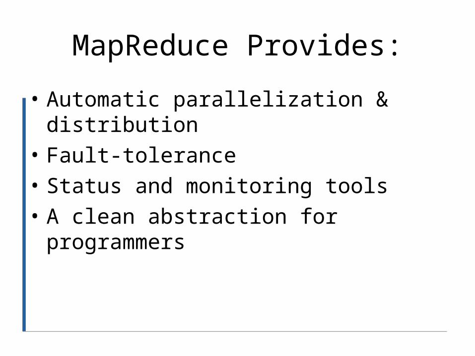
MapReduce Provides:
• Automatic parallelization & distribution
• Fault-tolerance• Status and monitoring tools• A clean abstraction for programmers

Programming Model
• Borrows from functional programming
• Users implement interface of two functions:
– map (in_key, in_value) ->
(out_key, intermediate_value) list
– reduce (out_key, intermediate_value list) ->
out_value list
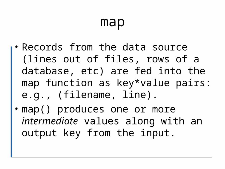
map
• Records from the data source (lines out of files, rows of a database, etc) are fed into the map function as key*value pairs: e.g., (filename, line).
• map() produces one or more intermediate values along with an output key from the input.

map (in_key, in_value) -> (out_key, intermediate_value) list
map

reduce
• After the map phase is over, all the intermediate values for a given output key are combined together into a list
• reduce() combines those intermediate values into one or more final values for that same output key
• (in practice, usually only one final value per key)
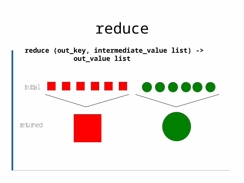
reducereduce (out_key, intermediate_value list) ->
out_value list
returned
initial

Data store 1 Data store nmap
(key 1, values...)
(key 2, values...)
(key 3, values...)
map
(key 1, values...)
(key 2, values...)
(key 3, values...)
Input key*value pairs
Input key*value pairs
== Barrier == : Aggregates intermediate values by output key
reduce reduce reduce
key 1, intermediate
values
key 2, intermediate
values
key 3, intermediate
values
final key 1 values
final key 2 values
final key 3 values
...

Parallelism
• map() functions run in parallel, creating different intermediate values from different input data sets
• reduce() functions also run in parallel, each working on a different output key
• All values are processed independently
• Bottleneck: reduce phase can’t start until map phase is completely finished.
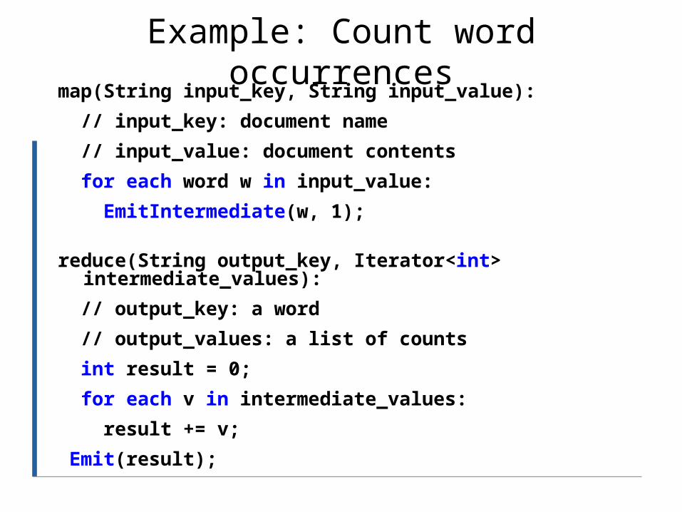
Example: Count word occurrencesmap(String input_key, String input_value):
// input_key: document name
// input_value: document contents
for each word w in input_value:
EmitIntermediate(w, 1);
reduce(String output_key, Iterator<int> intermediate_values):
// output_key: a word
// output_values: a list of counts
int result = 0;
for each v in intermediate_values:
result += v;
Emit(result);
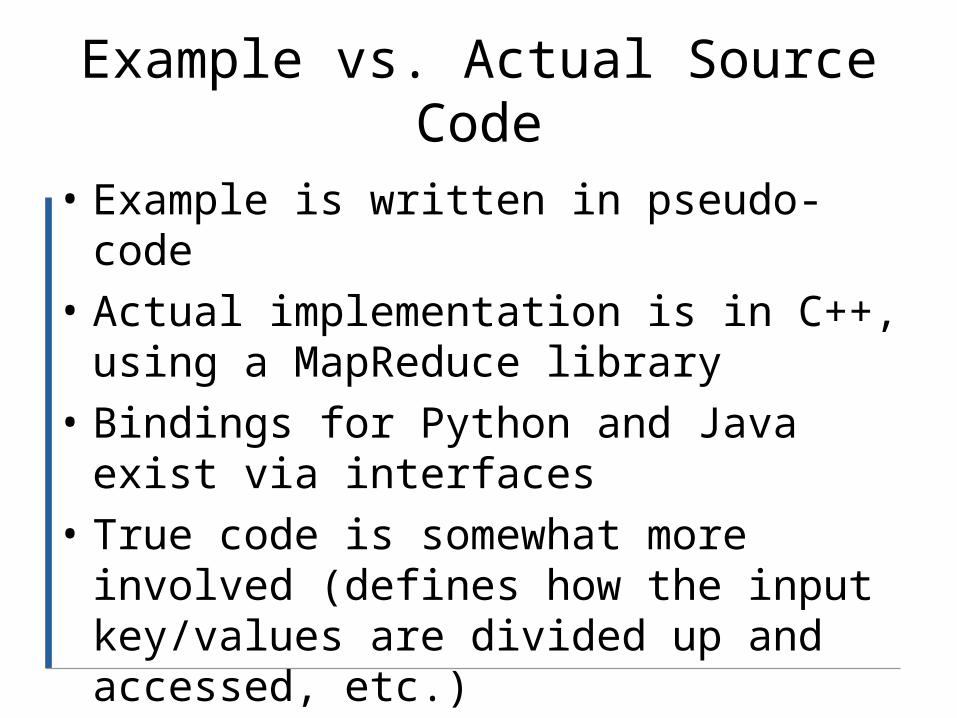
Example vs. Actual Source Code
• Example is written in pseudo-code• Actual implementation is in C++,
using a MapReduce library• Bindings for Python and Java exist via
interfaces• True code is somewhat more
involved (defines how the input key/values are divided up and accessed, etc.)

Locality
• Master program divvies up tasks based on location of data: tries to have map() tasks on same machine as physical file data, or at least same rack
• map() task inputs are divided into 64 MB blocks: same size as Google File System chunks
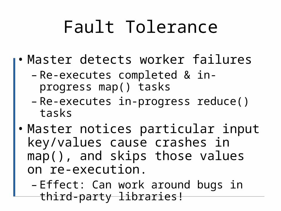
Fault Tolerance
• Master detects worker failures– Re-executes completed & in-progress
map() tasks– Re-executes in-progress reduce() tasks
• Master notices particular input key/values cause crashes in map(), and skips those values on re-execution.– Effect: Can work around bugs in third-
party libraries!
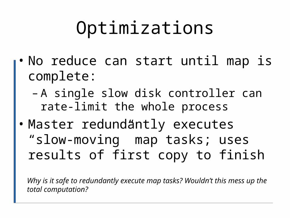
Optimizations
• No reduce can start until map is complete:– A single slow disk controller can rate-
limit the whole process
• Master redundantly executes “slow-moving” map tasks; uses results of first copy to finish
Why is it safe to redundantly execute map tasks? Wouldn’t this mess up the total computation?

Combining Phase
• Run on mapper nodes after map phase
• “Mini-reduce,” only on local map output
• Used to save bandwidth before sending data to full reducer
• Reducer can be combiner if commutative & associative

Combiner, graphically
Combiner replaces with:
Map output
To reducer
On one mapper machine:
To reducer
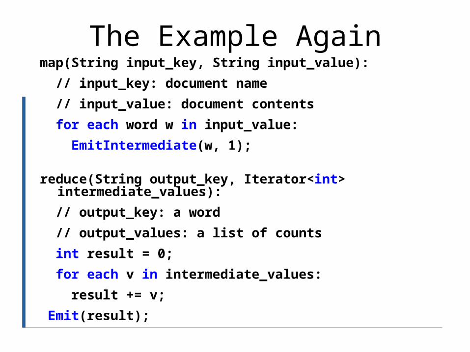
The Example Againmap(String input_key, String input_value):
// input_key: document name
// input_value: document contents
for each word w in input_value:
EmitIntermediate(w, 1);
reduce(String output_key, Iterator<int> intermediate_values):
// output_key: a word
// output_values: a list of counts
int result = 0;
for each v in intermediate_values:
result += v;
Emit(result);

MapReduce Conclusions
• MapReduce has proven to be a useful abstraction
• Greatly simplifies large-scale computations at Google
• Functional programming paradigm can be applied to large-scale applications
• Fun to use: focus on problem, let library deal w/ messy details

GFS
Some slides designed by Alex Moschuk, University of WashingtonRedistributed under the Creative Commons Attribution 3.0 license

Distributed Filesystems
• Support access to files on remote servers
• Must support concurrency• Can support replication and local
caching• Different implementations sit in
different places on complexity/feature scale
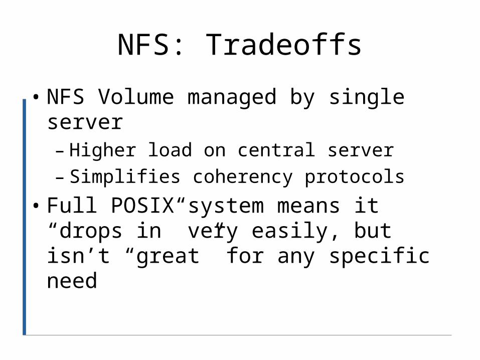
NFS: Tradeoffs
• NFS Volume managed by single server– Higher load on central server– Simplifies coherency protocols
• Full POSIX system means it “drops in” very easily, but isn’t “great” for any specific need

GFS: Motivation• Google needed a good distributed file
system– Redundant storage of massive amounts of data on
cheap and unreliable computers– … What does “good” entail?
• Why not use an existing file system?– Google’s problems are different from anyone
else’s• Different workload and design priorities• Particularly, bigger data sets than seen before
– GFS is designed for Google apps and workloads– Google apps are designed for GFS
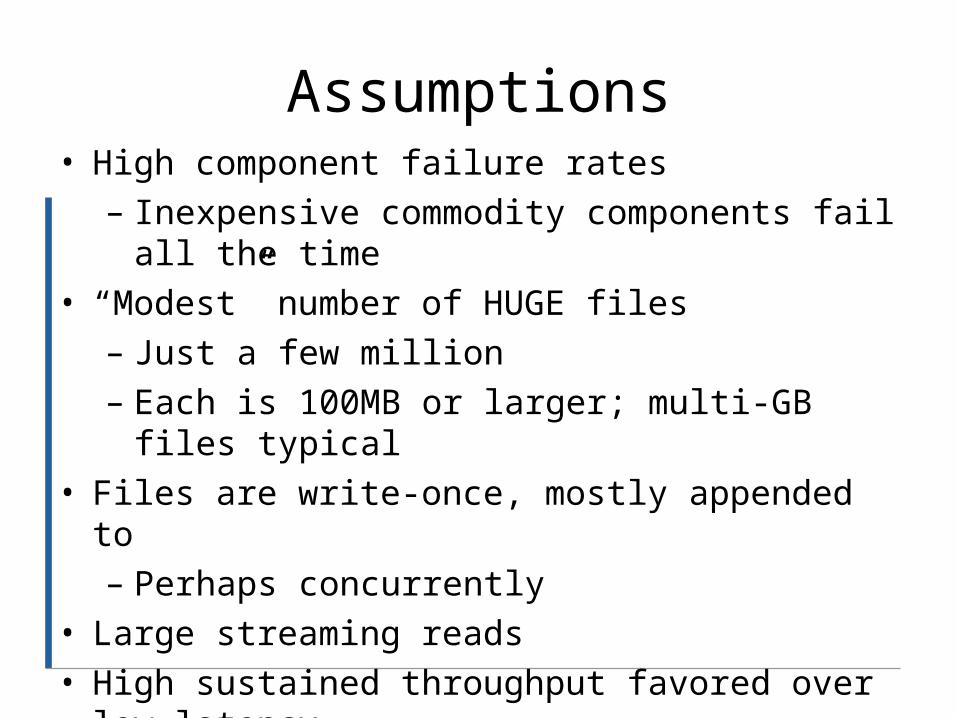
Assumptions• High component failure rates
– Inexpensive commodity components fail all the time
• “Modest” number of HUGE files– Just a few million– Each is 100MB or larger; multi-GB files
typical• Files are write-once, mostly appended to
– Perhaps concurrently• Large streaming reads• High sustained throughput favored over low
latency

GFS Design Decisions
• Files stored as chunks– Fixed size (64MB)
• Reliability through replication– Each chunk replicated across 3+ chunkservers
• Single master to coordinate access, keep metadata– Simple centralized management
• No data caching– Little benefit due to large data sets, streaming
reads• Familiar interface, but customize the API
– Simplify the problem; focus on Google apps– Add snapshot and record append operations

GFS Client Block Diagram
GFS-Aware Application
POSIX API GFS API
Regular VFS with local and NFS-supported files
Separate GFS view
Network stack
GFS Master
GFS Chunkserver
GFS Chunkserver
Specific drivers...
Client computer

GFS Architecture

Metadata (1/2)
• Global metadata is stored on the master– File and chunk namespaces– Mapping from files to chunks– Locations of each chunk’s replicas
• All in memory (64 bytes / chunk)– Fast– Easily accessible

Metadata (2/2)
• Master has an operation log for persistent logging of critical metadata updates– persistent on local disk– replicated– checkpoints for faster recovery

Mutations
• Mutation = write or append– must be done for all replicas
• Goal: minimize master involvement• Lease mechanism:
– master picks one replica as primary; gives it a “lease” for mutations
– primary defines a serial order of mutations– all replicas follow this order
• Data flow decoupled from control flow
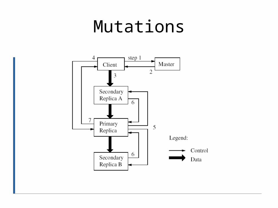
Mutations

Mutation Example
1. Client 1 opens "foo" for modify. Replicas are named A, B, and C. B is declared primary.
2. Client 1 sends data X for chunk to chunk servers3. Client 2 opens "foo" for modify. Replica B still
primary4. Client 2 sends data Y for chunk to chunk servers5. Server B declares that X will be applied before Y6. Other servers signal receipt of data7. All servers commit X then Y8. Clients 1 & 2 close connections9. B's lease on chunk is lost

Conclusion
• GFS demonstrates how to support large-scale processing workloads on commodity hardware– design to tolerate frequent component failures– optimize for huge files that are mostly
appended and read– feel free to relax and extend FS interface as
required– go for simple solutions (e.g., single master)
• GFS has met Google’s storage needs… win!

Technology Comparison
• Threads • MPI and PVM• Message Queues• Condor

Multithreading
• Single address space– More flexible structure– More possibilities of corruption
• Inherently single-machine based– Big performance on big systems

MPI, PVM
• Allow distributed control• Primarily used for message passing
and synchronization– Higher-level structures left up to
programmer– More overhead
• Reliability, high availability not built-in
Message Queues
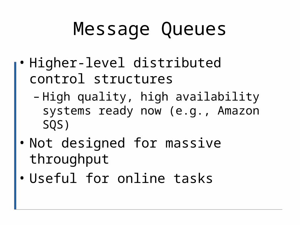
• Higher-level distributed control structures– High quality, high availability systems
ready now (e.g., Amazon SQS)
• Not designed for massive throughput• Useful for online tasks

Condor
• Grid scheduling / management system
• Works at a high level, like Hadoop• More general-purpose framework
– Requires programmers to control more aspects of the process
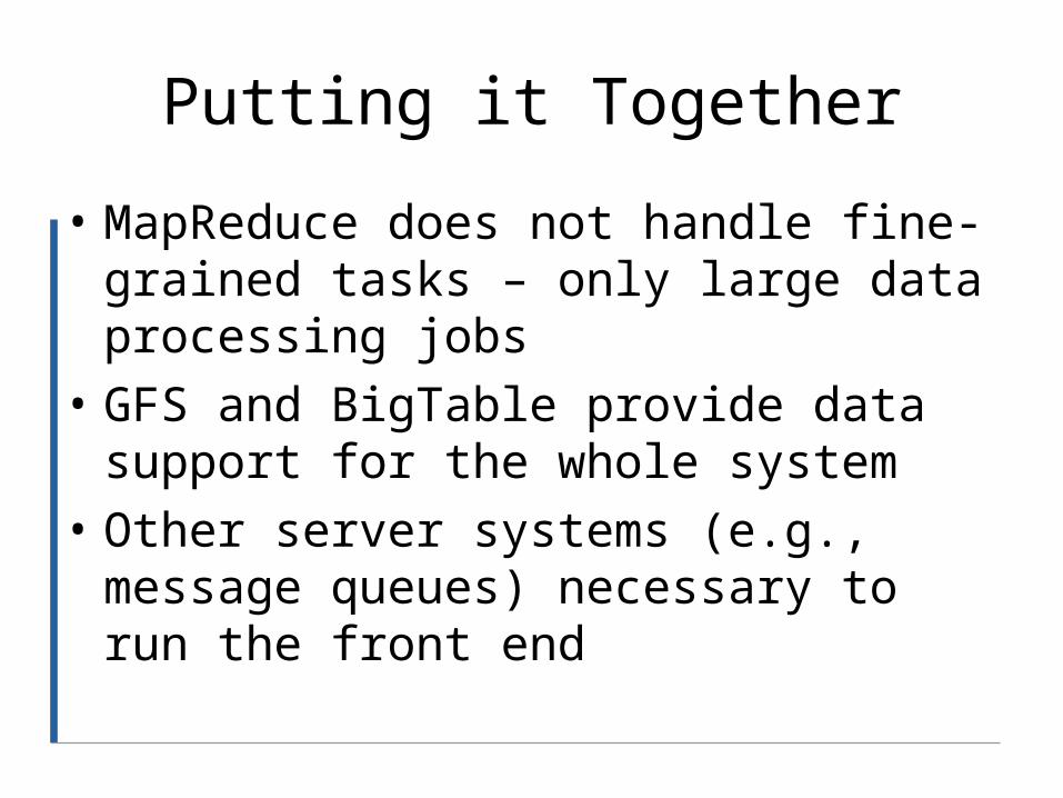
Putting it Together
• MapReduce does not handle fine-grained tasks – only large data processing jobs
• GFS and BigTable provide data support for the whole system
• Other server systems (e.g., message queues) necessary to run the front end

System Block Diagram
Front-end web servers
BigTable or other databases
Interactions with end-users
GFS storage
New raw data from Internet
MapReduce Batch Processes
Log dataOnline Processing Servers
Message queue

Conclusions
• A diverse set of applications centered around a common theme– Application layering simplifies
architecture– All work together to provide a variety of
general services– Applications must be designed in
particular ways to take advantage