maps in our heads: socio-political attitudes and demographic...
TRANSCRIPT

Maps in our Heads: Socio-political Attitudes andDemographic Awareness
Ryan D. Enos Tess Wise 1
1Department of Government, Harvard University; [email protected];[email protected]
Abstract
Research on the relationship between the awareness of social groups and socio-political at-titudes towards these groups has ignored a central attribute of groups: their geographiclocation. Instead researchers often (implicitly) assume that the proportion of an outgroupin certain population is the most important attribute of a group. We propose an alter-native measure of demographic contextual awareness: spatial accuracy which is a measureof the ability to place groups in space. This measure is consistent with theories of grouprepresentation in cognitive and evolutionary psychology and it resolves the tension betweenGroup Threat findings and the well-established fact that people are generally demographi-cally innumerate. In this paper, we present results from a preliminary investigation of spatialaccuracy. Using a novel online survey instrument which asks subjects to place social groupson a map of their local area, we find that survey respondents have a generally refined abilityto accurately locate social groups in space and that the ability of respondents to do so iscorrelated with political and intergroup attitudes.

1 Introduction
When an individual thinks about social groups what do they think about? What are the
most important features of a group? Is it the history of the group? The size of the group?
Cultural stereotypes about the group? In this paper, we argue that geographic location
is an overlooked salient feature of groups and that the “spatial awareness” of groups has
important socio-political implications.
Research on the relationship between the awareness of social groups and socio-political
attitudes towards these groups has ignored a central attribute of groups: their geographic
location. Instead researchers often (implicitly) assume that the population proportion of an
outgroup within a certain geographic area is the most important attribute of a group. We
propose an alternative measure of awareness: spatial accuracy. This measure is consistent
with theories of social cognition in cognitive and evolutionary psychology and resolves the
tension between Group Threat findings and the well-established fact that people are generally
demographically innumerate (see Wong (2007)). We suggest that studying spatial accuracy
can help to resolve contradictory findings across the broad “contextual effects” literature.
Using a novel online survey instrument which asks subjects to place social groups on
a map of their local area, we explore the relationship between spatial accuracy and socio-
political attitudes. We find that survey respondents have a generally refined ability to
accurately locate social groups in space. Additionally we explore some preliminary connec-
tions between this ability and socio-political attitudes. We find that the ability of white
respondents to accurately place “non-threatening” groups (whites and Asian Americans)
is correlated with higher values of racial resentment while the ability to accurately place
“threatening” groups (African Americans and Latinos) does not predict higher values of
racial resentment. Alternatively, the ability to accurately place outgroups is correlated with
a higher likelihood of claiming to “share the political views” of these groups – suggesting,
perhaps, that racially conservative respondents rely on abstract stereotypes of outgroups,
even when locating these groups spatially. These findings suggest that the “maps in our
1
heads” reveal important insights about our socio-political attitudes and are worthy of fur-
ther investigation.
This paper proceeds as follows: First, we discuss the large literature of groups, context,
and the measurement of threat and why spatial location fits naturally in this literature.
Second, we describe our survey design. Then, we discuss the measurement of spatial accuracy
and its relationship to socio-political attitudes. We close by discussing the implications of
our findings and future extensions.
2 Background
Since at least Key’s (1949) seminal work, there has been an interest in how demographic
context affects political behavior. Although this literature is certainly nested in a wider
literature encompassing deep research agendas in economics, psychology, and sociology, in
the political science literature the study of demographic context has come to focus on a loose
collection of concepts that are collectively termed “racial threat”. In this section we point
out that while the mechanisms through which racial threat operates have been under much
debate, there has been less debate over the use of demographic proportions as the method for
modeling demographic context. Recent work, however, has highlighted fruitful approaches
such as considering perceptions of demographics and using psychologically relevant areal
units (Wong, Bowers, Williams, and Drake 2012). Our work builds on the insights from this
work, but also proposes a new independent variable: spatial accuracy, which we argue is
more consistent with the cognitive processes underlying the way humans think about social
groups.
Nearly all studies of racial threat, at least implicitly, are based on a model that individual
political behavior is a function of the presence of a geographically proximate racial or ethnic
outgroup. The outcome behaviors of interest are usually voting (turnout or vote choice) or
intergroup attitudes. There is wide divergence in the mechanism(s) through which racial
2
threat operates. Proposed mechanisms range from rational responses to material threat
(Bobo 1983), to the competition over descriptive representation (Spence and McClerking
2010), stimulation of old-fashioned racial stereotypes (Giles and Buckner 1993), manipulation
by interested elites (Key 1949), or preservation of “white power” (Voss 1996) – to name but
a very partial list.
While the mechanisms have varied, the independent variables considered have remained
remarkably constant: studies of of demographic context and racial threat usually explicitly
or implicitly assume that individuals are reacting to the concentration of an outgroup in their
proximate area. Despite the predominance of this independent variable, there is increasing
evidence that very few people have anything close to an accurate sense of group population
proportions (Nadeau, Niemi, and Levine 1993, Sigelman and Niemi 2001, Gallagher 2003,
Alba, Rumbaut, and Marotz 2005, Wong 2007, Martinez, Wald, and Craig 2008). This
presents a puzzle: How can individuals be reacting strongly to the proportions of outgroups
when they are not aware of these proportions? Our new measure, spatial accuracy represents
a step towards resolving this tension by showing knowledge of group location is correlated
with both racial resentment and feelings of shared political identity.
While we are the first scholars to consider spatial accuracy, we are building on a strong
tradition of other scholars who have recently brought new insight to the study of demographic
context and socio-political attitudes. In studies of demographic proportions, some models
such as Gay (2006) include characteristics of the outgroup, such as income, as mediators
of the effect of population proportion. Other models, such as the one developed byHopkins
(2010) use changes in the concentration of immigrants at the zip code and county levels
combined with media attention as the independent variable of interest in explaining attitudes
towards immigrants.
Recent work by Wong et al. (2012) highlights the inconsistency between psychologically
relevant space and spaced measured by researchers. Wong et al. (2012) brings in a psycho-
logical model which relies on the difference between perceptions of demographic proportions
3
and objective demographics. Their research finds that within pairs of white respondents in
similar objective racial contexts (as measured by census data), the person perceiving more
blacks tended to be the person with higher racial resentment. Our theory of spatial accuracy
builds on this work by considering perceptions of location and also avoids the problem of
psychologically relevant space by presenting individuals with un-bounded and manipulable
maps, allowing the respondent to focus on what is relevant to them.
2.1 The cognitive basis of racial threat and spatial accuracy
Scholars (Wong 2007, Wong 2010, Wong et al. 2012) have begun to explore the psychological
underpinnings of responses to group threat. We too are interested in the social cognition that
translates the presence of an outgroup into something threatening that invokes a behavioral
response. In other words, what is it about outgroups that concerns people?
Theories of behavioral responses to the presence of an outgroup rest on models of the
“schema” that individuals attach to an outgroup. Schema are “mental representations of
a category, that is, a class of objects that we believe belong together” (Kunda 1999, p.16).
Schema are comprised of the attributes we attach to objects (e.g. people and groups). These
attributes can be physical qualities, such as skin color, or social qualities, such as propensity
for crime. Attributes are of varying accessibility: sometimes when presented with a group,
one attribute might be the first and most powerful thing we associate with that group. In
the context of the Racial Threat literature, when evaluating the “threat” of a group, an
individual will consider the attributes of that group, some of which may be more or less
accessible than others.
Theories of context, usually implicitly, model the population proportion of a group as the
most accessible attribute an individual can use to evaluate the “threat” of a group. In other
words, when individuals consider an outgroup in a political context, the most important
feature of the outgroup is the proportion of that outgroup in the population. Here, we argue
that an attribute that is also very important, perhaps more important, is the spatial location
4
of the outgroup. In other words, when people think about a group, the first thing that comes
to mind is not “how big is that group?”, rather it is “where is that group?”.
The assumption in the literature that outgroup proportions are the most important
attribute of a group may come from rational actor models, in which an individual has no
incentive to react to a group until they reach a large enough proportion of the population to
threaten the interests of the individual – in politics, this usually will mean enough to enter
a minimal winning coalition.
To illustrate why this assumption is unnecessary see the example of a recent prominent
finding on threat: Hopkins (2010) makes an important contribution to the literature by
connecting threat to prominent theories in political science and psychology by modeling
threat from Latino immigrants in the United States as a function of signals from policy
elites and changes in population levels. However, what Hopkins does not show (and is not
necessary for the purposes of his paper) is the schema that individuals attach to immigrants
that make them threatening. It could be that the changes in concentration prompt people
to think about how many immigrants are in their local area, but it also could prompt
individuals to think about where immigrants can be found in their local area. Here we argue
that the question of where? is more likely what individuals are asking and that modeling the
cognition of threat in this manner helps to resolve the inconsistency between racial threat
findings like Hopkins (2010) and demographic innumeracy findings like Wong (2007).
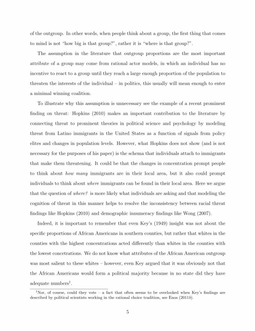
Indeed, it is important to remember that even Key’s (1949) insight was not about the
specific proportions of African Americans in southern counties, but rather that whites in the
counties with the highest concentrations acted differently than whites in the counties with
the lowest concetrations. We do not know what attributes of the African American outgroup
was most salient to these whites – however, even Key argued that it was obviously not that
the African Americans would form a political majority because in no state did they have
adequate numbers1.
1Nor, of course, could they vote – a fact that often seems to be overlooked when Key’s findings aredescribed by political scientists working in the rational choice tradition, see Enos (2011b).
5

With the assistance of modern cognitive science, we argue that the more likely explanation
is that these whites were more concerned with the location of these African Americans than
with their numbers.
2.2 Location and social cognition
In our theory of spatial accuracy we focus on space, because it has been shown that space
occupies a central role in human cognition – indeed, “as humans, our ability to operate in
large-scale space has been crucial to our adaptation and survival (Maguire 2006, p. 131).”
There is evidence that the human ability for spatial navigation has evolved into the structure
of our episodic memory (Burgess, Maguire, and O’keefe 2002), which is a crucial aspect of
the unique human cognitive function. It is easy to imagine scenarios that illustrate this –
in developing the capacity to process objects important to survival, for example food and
enemies, while size may certainly have been important, a precise sense of size was probably
not as important as a precise sense of spatial location: as long as a person knew there was
enough food to eat, the exact number was not important to survival, but to not remember
the precise location of the food may have been a clear threat to survival. The extension of
the importance of space to groups is easy to see: a person could survive with an imprecise
knowledge of size – simply knowing if any enemy is more or less numerous than your group
might suffice – but not knowing precisely whether you had entered the enemies territory
might be fatal. In a certain respect, location can be thought of as a heuristic, likely highly
developed, for answering crucial questions about safety and other utility inputs.
We emphasize that we are not making a direct analogy between group conflict in the
human evolutionary past and modern political conflict (although some scholars have recently
done just that, see Haidt (2012)), rather we are emphasizing that groups and space are central
components of human cognition and when considering the central role of groups in political
behavior, space should also take center stage.
Moreover though, the usefulness space and groups as heuristics likely take on an even
6
more crucial role when an individual is in complex urban environments such as those in which
most people now live. Cities, with their complex spatial structures and dense activities put a
great strain on human cognition – there are simply more environmental inputs than a person
can process, making space a valuable heuristic. Stanley Milgrim described the cognitive
strain induced by cities as “overload” and speculated that a good deal of human activity
that characterized urban environments, including ethnocentrism, could be attributed to the
need to reduce overload (Milgim 1970). So not only do groups and space have a central role
in human cognition generally, they become perhaps more central in urban environments –
the environment of most human activity and the scene of the greatest ethnic diversity.
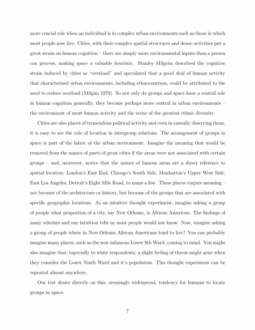
Cities are also places of tremendous political activity and even in casually observing them,
it is easy to see the role of location in intergroup relations. The arrangement of groups in
space is part of the fabric of the urban environment. Imagine the meaning that would be
removed from the names of parts of great cities if the areas were not associated with certain
groups – and, moreover, notice that the names of famous areas are a direct reference to
spatial location: London’s East End, Chicago’s South Side, Manhattan’s Upper West Side,
East Los Angeles, Detroit’s Eight Mile Road, to name a few. These places conjure meaning –
not because of the architecture or history, but because of the groups that are associated with
specific geographic locations. As an intuitive thought experiment, imagine asking a group
of people what proportion of a city, say New Orleans, is African American. The findings of
many scholars and our intuition tells us most people would not know. Now, imagine asking
a group of people where in New Orleans African Americans tend to live? You can probably
imagine many places, such as the now infamous Lower 9th Ward, coming to mind. You might
also imagine that, especially to white respondents, a slight feeling of threat might arise when
they consider the Lower Ninth Ward and it’s population. This thought experiment can be
repeated almost anywhere.
Our test draws directly on this, seemingly widespread, tendency for humans to locate
groups in space.
7
3 Design
Prior to beginning this research, we received permission from our university’s Committee on
the Use of Human Subjects in Research.
We implemented a web-based survey that asks respondents to place groups in their
community. Subjects were recruited using Amazon’s Mechanical Turk (see Berinsky, Huber,
and Lenz (2012))2.
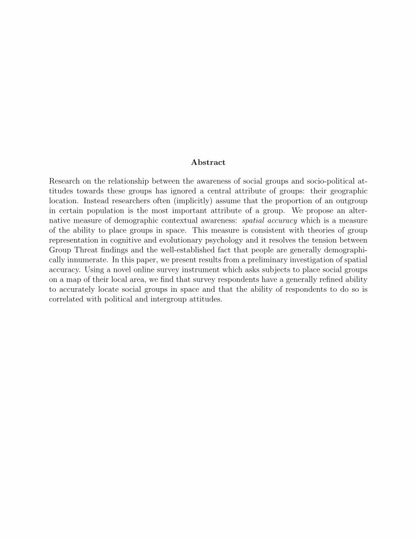
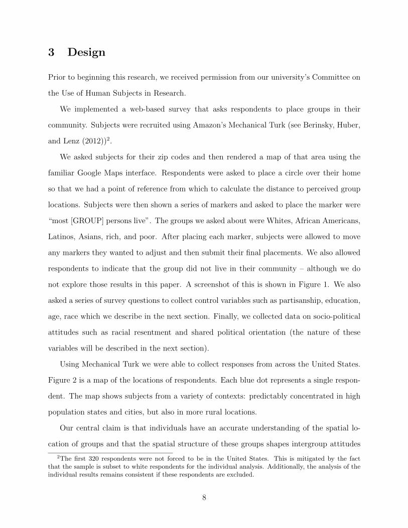
We asked subjects for their zip codes and then rendered a map of that area using the
familiar Google Maps interface. Respondents were asked to place a circle over their home
so that we had a point of reference from which to calculate the distance to perceived group
locations. Subjects were then shown a series of markers and asked to place the marker were
“most [GROUP] persons live”. The groups we asked about were Whites, African Americans,
Latinos, Asians, rich, and poor. After placing each marker, subjects were allowed to move
any markers they wanted to adjust and then submit their final placements. We also allowed
respondents to indicate that the group did not live in their community – although we do
not explore those results in this paper. A screenshot of this is shown in Figure 1. We also
asked a series of survey questions to collect control variables such as partisanship, education,
age, race which we describe in the next section. Finally, we collected data on socio-political
attitudes such as racial resentment and shared political orientation (the nature of these
variables will be described in the next section).
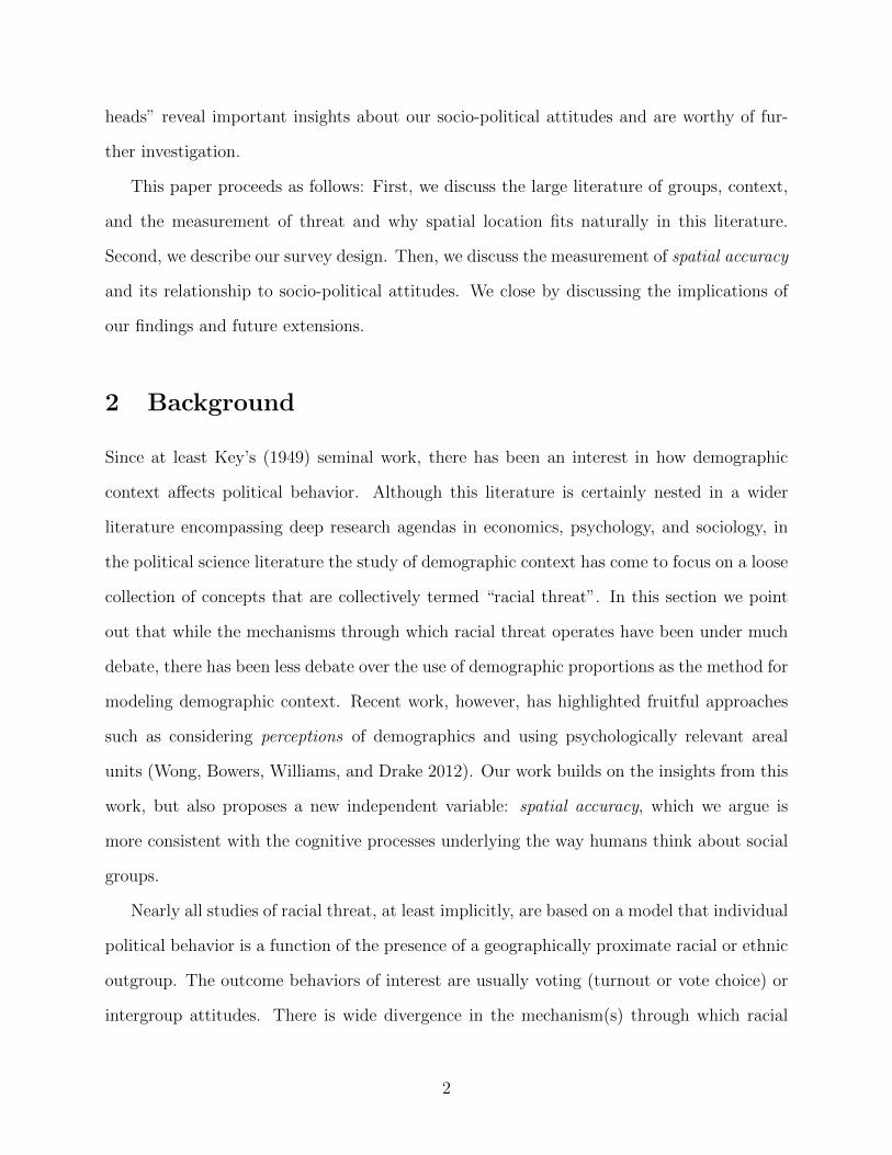
Using Mechanical Turk we were able to collect responses from across the United States.
Figure 2 is a map of the locations of respondents. Each blue dot represents a single respon-
dent. The map shows subjects from a variety of contexts: predictably concentrated in high
population states and cities, but also in more rural locations.
Our central claim is that individuals have an accurate understanding of the spatial lo-
cation of groups and that the spatial structure of these groups shapes intergroup attitudes
2The first 320 respondents were not forced to be in the United States. This is mitigated by the factthat the sample is subset to white respondents for the individual analysis. Additionally, the analysis of theindividual results remains consistent if these respondents are excluded.
8
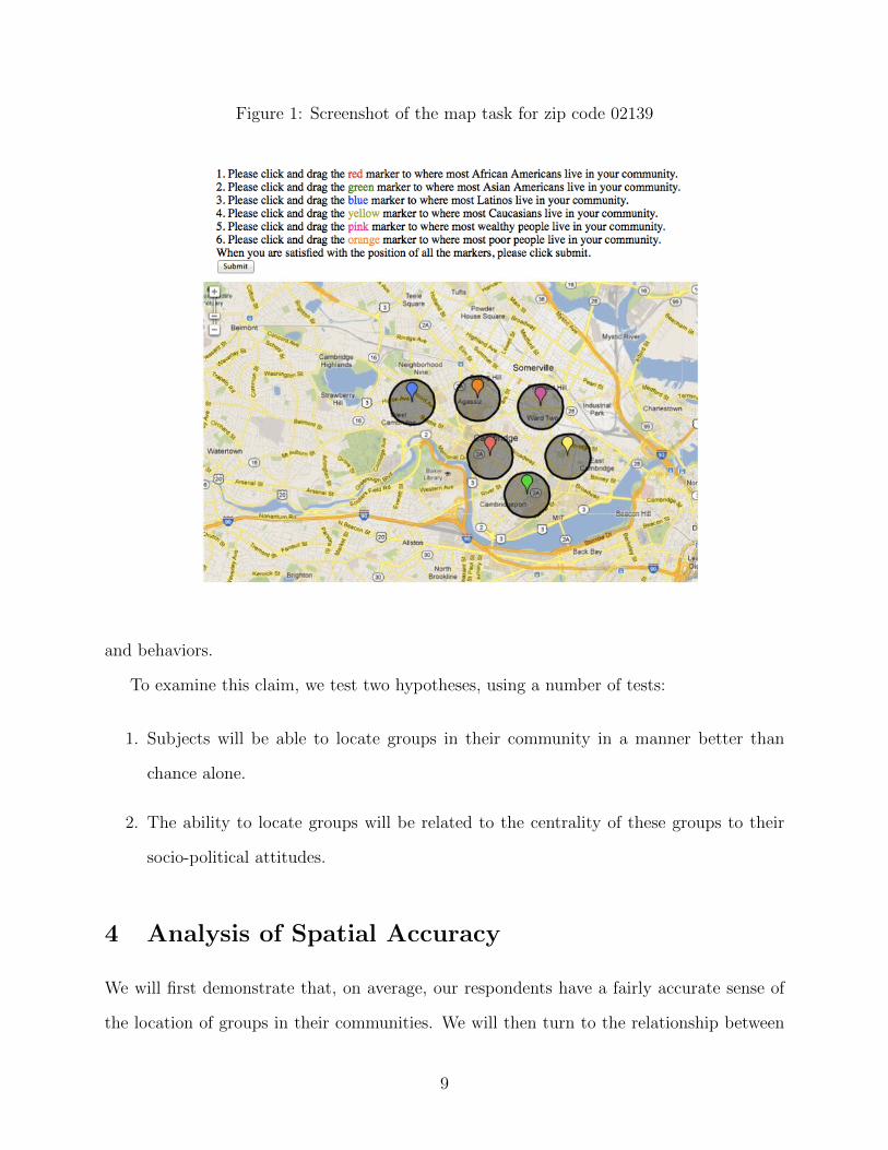
Figure 1: Screenshot of the map task for zip code 02139
and behaviors.
To examine this claim, we test two hypotheses, using a number of tests:
1. Subjects will be able to locate groups in their community in a manner better than
chance alone.
2. The ability to locate groups will be related to the centrality of these groups to their
socio-political attitudes.
4 Analysis of Spatial Accuracy
We will first demonstrate that, on average, our respondents have a fairly accurate sense of
the location of groups in their communities. We will then turn to the relationship between
9

Figure 2: Map of respondents’ homes
●
●
●
●
●
●
●
●
●
●
●
●●
●
●●
●
●
●
●
●
●
●
●
●
●●
●
●
●
●●
●
●
●
●
●●
●
●
●
●
●
●
●
●
●
●
●
●
●
●
●● ●
●
●
●
●
●
●
●
●
●
●
●
●
●
●
●
●
●
●
●
●
●
●
●
●
●
●
●
●
●
●
●
●
●
●
●
●
●
●
●
●
●
●
●
●
●
●
●
●
●
●
●
●
●●
●
●
●
●
●
●
●
●
●
●
●
●
●
●
●
●
●
●
●
●
●●
●
●
●
●
●
●
●
●
●
●
●
●
●
●
●
●
●
●
●
●
●
●
●
●
●
●
●
●
●
●
●
●
● ●
●
●
●
●
●
●
●
●
●
●
●
●
●
●
●
●
●
●
●
●
●●
●
●
●
●
●
●
●
●
●
●
●
●●
●
●
●
●
●
●
●
●
●
●
●
●●
●
●●
●
●
●
●
●
●
●
●
●
●
●
●
●
●
●
●
●
●
●
●
●
●
●
●
●
●
●
●
●
●
●
●
●
●
●
●
●
●
●
●
●
●
●
●
●●
●
●
●
●
●
●
●
●●
●
●
●
●
●
●
●
●
●
●
●
●
●
●
●
●
●
●
●
●
●
●
●
●
●
●
●
●
●
●
●
●
●
●
●
●
●
●
●
●●
●
●
●
●
●
●
●
●
●
●●
●
●●
●
●
●
●
●
●●
●●
●
●
●
●●
●
●
● ●
●
●
●
●
●●
●
●
●
●
●●
●
●
●
●
●
●
●
●
●
●
●
●
●
●
●●
●
●
●
●
●
●
●
●
●
●
●
●●
●
●
●
●
●
●
●
●
●
●
●
●
●
●
●
●
●
●●
●
●
●
●
●
●
●
●
●
●
●
●
●
●
●
●
●
●
●
●
●●
● ●
●
●
●
●
●
●
●
●●
●●
●
●
●
●
●
●
●
●
●
●
●
●
●
●
●
●
●
●
●●
●●
●
●
●
●
●
●
●
●
●
●
●
●
●
●
●
●
●
●
●
●
●
●●
●
●
●●
●
●
●
● ●
●
●●
●
●
●
●
●
●●
●
●
●
●
●
●
●
●
●
●
●
●
●
●
●
●
●
●
●
●
●
●
●
●
●
●
●
●
●
●
●
●
●
●
●
●
●
●
●
●●
●
●
●
●
●●
●
●
●●
●
●
●
●
●
●
●●
●
●
●
●
●
●
●
●
●●
●
●
●
●
●
●
●
●
●
●
●
●
●
●
●
●
●
●
●
●
●
●
●
●
●
●
●
●
●
●
●
●
●
●
●
●
●
●
●
●
●
●
●
●
●
●
●●●
●
●
●
● ●
●
●
●
●
●
●
●●
●●
●
●●
●
●
●
●
●
●
●
●
●
●
●
●
●
●
●
●
●
●
●
●
●
●
●
●
●
●
●
●●
●
●
●●
●
●●
●
●●
●
●
●
●
●
●
●
●●
●
●
●
●
● ●
●
●
●
●
●
●
●
●
●
●
●
●
●
●
●
●
●
●
●
●
●
●
●
●
●●
●
●
●
●
●
●
●
●
●
●
●
●
●
●●
●
●●
●
●
●
●
●
●
●
●
●
●
●
●
●
●●
●
●
●
●
●●
●
●
●
●
●
●●
●
●
●
●
●
●
●
●
●
●
●
●
●
●
●
●
●
●
●
●
●
●
●
●
●●
●
●
●
●
● ●
●
●
●
●
●
●
●
●
●
●
●
●
●
●
●
●
●
●
● ●●
●
●
●
●
●
●
●
●
●
●
●
Each blue dot is the location of the home of a respondent.
accuracy and other individual level variables.
4.1 Defining Accuracy
Our central claim is that individuals can accurately describe the spatial location of groups. In
demonstrating this claim, we make several choices. One of the most consequential, perhaps,
is to define an areal unit in which to define a population to measure. While Census and
other administrative units may not fit with with individual constructs of neighborhood (e.g.
Wong et al. (2012)), in order to measure accuracy we need an areal unit to which we can
attach Census data. Here we report results for Census Tracts because it is a commonly used
unit. In essence, our measures of accuracy are all simply whether or not a respondent placed
a group inside the Census Tract where that group was most likely to be found. Of course,
10
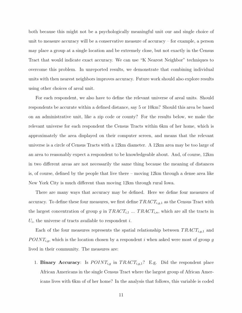
both because this might not be a psychologically meaningful unit our and single choice of
unit to measure accuracy will be a conservative measure of accuracy – for example, a person
may place a group at a single location and be extremely close, but not exactly in the Census
Tract that would indicate exact accuracy. We can use “K Nearest Neighbor” techniques to
overcome this problem. In unreported results, we demonstrate that combining individual
units with then nearest neighbors improves accuracy. Future work should also explore results
using other choices of areal unit.
For each respondent, we also have to define the relevant universe of areal units. Should
respondents be accurate within a defined distance, say 5 or 10km? Should this area be based
on an administrative unit, like a zip code or county? For the results below, we make the
relevant universe for each respondent the Census Tracts within 6km of her home, which is
approximately the area displayed on their computer screen, and means that the relevant
universe is a circle of Census Tracts with a 12km diameter. A 12km area may be too large of
an area to reasonably expect a respondent to be knowledgeable about. And, of course, 12km
in two different areas are not necessarily the same thing because the meaning of distances
is, of course, defined by the people that live there – moving 12km through a dense area like
New York City is much different than moving 12km through rural Iowa.
There are many ways that accuracy may be defined. Here we define four measures of
accuracy. To define these four measures, we first define TRACTi,g,1 as the Census Tract with
the largest concentration of group g in TRACTi,1 ... TRACTi,n, which are all the tracts in
Ui, the universe of tracts available to respondent i.
Each of the four measures represents the spatial relationship between TRACTi,g,1 and
POINTi,g, which is the location chosen by a respondent i when asked were most of group g
lived in their community. The measures are:
1. Binary Accuracy: Is POINTi,g in TRACTi,g,1? E.g. Did the respondent place
African Americans in the single Census Tract where the largest group of African Amer-
icans lives with 6km of of her home? In the analysis that follows, this variable is coded
11
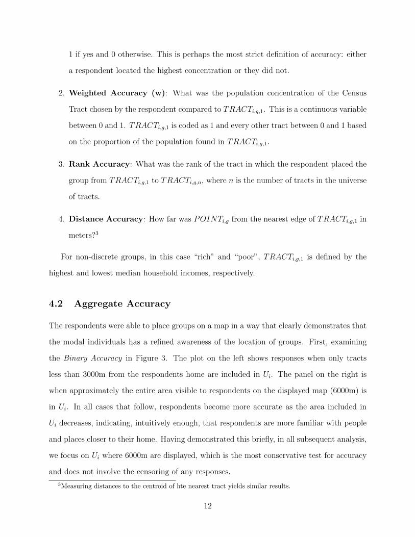
1 if yes and 0 otherwise. This is perhaps the most strict definition of accuracy: either
a respondent located the highest concentration or they did not.
2. Weighted Accuracy (w): What was the population concentration of the Census
Tract chosen by the respondent compared to TRACTi,g,1. This is a continuous variable
between 0 and 1. TRACTi,g,1 is coded as 1 and every other tract between 0 and 1 based
on the proportion of the population found in TRACTi,g,1.
3. Rank Accuracy: What was the rank of the tract in which the respondent placed the
group from TRACTi,g,1 to TRACTi,g,n, where n is the number of tracts in the universe
of tracts.
4. Distance Accuracy: How far was POINTi,g from the nearest edge of TRACTi,g,1 in
meters?3
For non-discrete groups, in this case “rich” and “poor”, TRACTi,g,1 is defined by the
highest and lowest median household incomes, respectively.
4.2 Aggregate Accuracy
The respondents were able to place groups on a map in a way that clearly demonstrates that
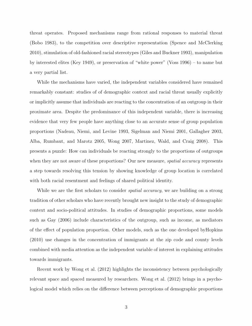
the modal individuals has a refined awareness of the location of groups. First, examining
the Binary Accuracy in Figure 3. The plot on the left shows responses when only tracts
less than 3000m from the respondents home are included in Ui. The panel on the right is
when approximately the entire area visible to respondents on the displayed map (6000m) is
in Ui. In all cases that follow, respondents become more accurate as the area included in
Ui decreases, indicating, intuitively enough, that respondents are more familiar with people
and places closer to their home. Having demonstrated this briefly, in all subsequent analysis,
we focus on Ui where 6000m are displayed, which is the most conservative test for accuracy
and does not involve the censoring of any responses.
3Measuring distances to the centroid of hte nearest tract yields similar results.
12
This red bars in Figure 3 represent the percent of times that respondents chose TRACT1g.
For example, when locating TRACT1white, respondents correctly located that tract over 20%
of the time. The gray bars represent the proportion of times that TRACT1g would be
chosen at random by a person choosing among n tracts. We constructed these measures by
weighting each tract by its land-area and then randomly simulating 1000 draws from Ui for
each respondent. This simulation reflects that a person that truely was choosing randomly
would be more likely to choose spatially large tracts simply because they occupy more space
on the map.4 This demonstrates that a person choosing randomly likely would have selected
TRACT1white around 6% of the time. These results clearly demonstrate that subjects were
not just choosing at random.
At both distances, for every group, a T-test for the difference of means between the
simulated accuracy and the observed accuracy yields p < 10−10, indicating difference of
means that we obtain would be extremely unlikely to observe if respondents were truly
choosing randomly. This might be considered an impressive demonstration of accuracy,
given the strict definition of accuracy used here: for example, a respondent may have chosen
TRACT2white, where TRACT2white has a white population of 99 and TRACT1white has a
population of 100, but this respondent would still be scored 0.
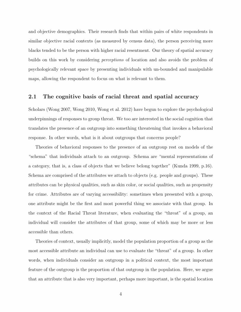
To give more weight to approximately correct answers such as this example, we turn to
Weighted Accuracy in Figure 4. In this figure, we demonstrate that the average respondent
chose a tract with a high weight. For example, when asked to choose a location where most
“rich” people live, the average respondent chose the location where the median income was
almost 80% of the highest income in U .
Of course, Accuracy Weight, like many of the measures used in this paper, is context
dependent: for example, if a group is perfectly evenly distributed across tracts, then a
respondent cannot help but choose a tract with w = 1 even if they are guessing at random.
On the other hand, in a universe where the population is very unevenly distributed, say
4The substance of the results is completely unchanged if tracts are given equal weight in the simulation.
13

Figure 3: Binary accuracy by group compared to expected accuracy
(a) Distance = 6000 meters
white black asian latino rich poor
0.00
0.05
0.10
0.15
0.20
0.25
white black asian latino rich poor
0.00
0.05
0.10
0.15
0.20
0.25
(b) Distance = 3000 meters
white black asian latino rich poor0.
000.
050.
100.
150.
200.
25white black asian latino rich poor
0.00
0.05
0.10
0.15
0.20
0.25
Binary accuracy by Group are the red bars. The expected accuracy, calculated by simulated draws from amap accounting for land area of each tract are gray bars.
pop(TRACT1,white) > 2 ∗ pop(TRACT2,white), then even if a person chose TRACT2,white, the
weight of the tract they chose would be no greater than w = .50. We attempt to separate
these situations by simulating random draws from the distribution of weights that each
respondent could possibly make and comparing these to the actual selections.
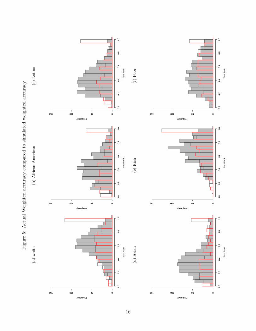
In Figure 5 we displays the distributions of means from 1000 simulated draws for each
respondent (gray) against the distribution of actual responses (red) by target group. In
all cases, the actually responses are shifted considerably to the right, indicating that the
respondents chose the higher weighted Census Tracts much more often than they would have
if they were just guessing at random. It is notable though that when the target population
is both African American and Asian American, the distributions have fat tails, indicating
that they respondents not only did better than would be expected at random, but at times
also did worse than would be expected at random. A Wilcox Rank Sum test for a difference
in the actual and simulated distributions yields p < .005 for each group, indicating that we
14

Figure 4: Weighted accuracy by group
white black asian latino rich poor
0.0
0.2
0.4
0.6
0.8
1.0
Weighted accuracy by Group: the average population of Group G in the Tract containing POINTi,g asfraction of the population in TRACTi,g,1.
would be very unlikely to observe distributions this different if the distributions were really
the same.
We also consider Rank Accuracy – the rankings of Census Tracts from 1...n. This does
not have the features of allowing for relative population differences like measuring Weighted
Accuracy, but is ordinal so it allows us to distinguish between tracts of lesser or greater
concentrations of the group. Of course, the meaning of a ranking is also context dependent, so
that finding the highest concentration tract when n = 1 cannot distinguish spatial awareness
from guessing. However, using similar strategies to those above, we demonstrate that our
typical respondent was clearly not guessing.
In Figure 6 we display the number of tracts in Ui on the x-axis and the rank of the tract
selected by the respondent on the y-axis. The points are jittered for display purposes. Points
in the lower right are respondents that either have a very developed spatial awareness or are
quite lucky. Points in the lower left are responses which are more difficult to distinguish
guessing from accuracy because of the low number of tracts in Ui. However, the general
15
Fig
ure
5:A
ctual
Wei
ghte
dac
cura
cyco
mpar
edto
sim
ula
ted
wei
ghte
dac
cura
cy
(a)
wh
ite
Frequency
0.0
0.2
0.4
0.6
0.8
1.0
050100150
Trac
t Ran
k
Frequency
0.0
0.2
0.4
0.6
0.8
1.0
050100150
(b)
Afr
ican
Am
eric
an
Frequency
0.0
0.2
0.4
0.6
0.8
1.0
050100150
Trac
t Ran
kFrequency
0.0
0.2
0.4
0.6
0.8
1.0
050100150
(c)
Lati
no
Frequency
0.0
0.2
0.4
0.6
0.8
1.0
050100150
Trac
t Ran
k
Frequency
0.0
0.2
0.4
0.6
0.8
1.0
050100150
(d)
Asi
an
Frequency
0.0
0.2
0.4
0.6
0.8
1.0
050100150
Trac
t Ran
k
Frequency
0.0
0.2
0.4
0.6
0.8
1.0
050100150
(e)
Ric
h
Frequency
0.0
0.2
0.4
0.6
0.8
1.0
050100150
Trac
t Ran
k
Frequency
0.0
0.2
0.4
0.6
0.8
1.0
050100150
(f)
Poor
Frequency
0.0
0.2
0.4
0.6
0.8
1.0
050100150
Trac
t Ran
k
Frequency
0.0
0.2
0.4
0.6
0.8
1.0
050100150
16
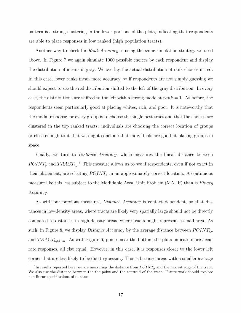
pattern is a strong clustering in the lower portions of the plots, indicating that respondents
are able to place responses in low ranked (high population tracts).
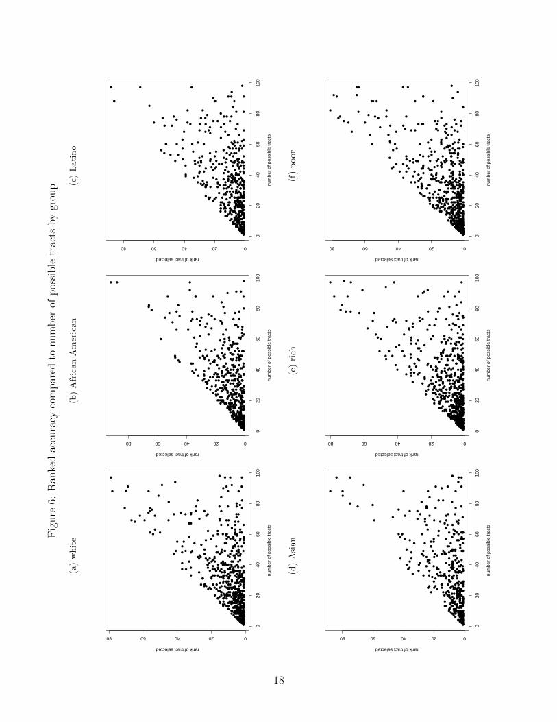
Another way to check for Rank Accuracy is using the same simulation strategy we used
above. In Figure 7 we again simulate 1000 possible choices by each respondent and display
the distribution of means in gray. We overlay the actual distribution of rank choices in red.
In this case, lower ranks mean more accuracy, so if respondents are not simply guessing we
should expect to see the red distribution shifted to the left of the gray distribution. In every
case, the distributions are shifted to the left with a strong mode at rank = 1. As before, the
respondents seem particularly good at placing whites, rich, and poor. It is noteworthy that
the modal response for every group is to choose the single best tract and that the choices are
clustered in the top ranked tracts: individuals are choosing the correct location of groups
or close enough to it that we might conclude that individuals are good at placing groups in
space.
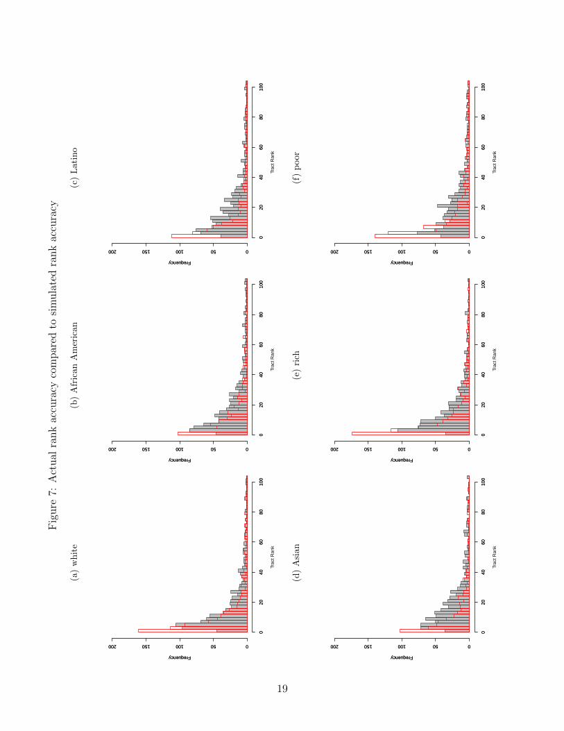
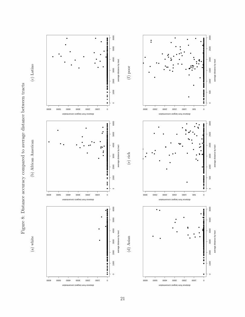
Finally, we turn to Distance Accuracy, which measures the linear distance between
POINTg and TRACT1g.5 This measure allows us to see if respondents, even if not exact in
their placement, are selecting POINTg in an approximately correct location. A continuous
measure like this less subject to the Modifiable Areal Unit Problem (MAUP) than is Binary
Accuracy.
As with our previous measures, Distance Accuracy is context dependent, so that dis-
tances in low-density areas, where tracts are likely very spatially large should not be directly
compared to distances in high-density areas, where tracts might represent a small area. As
such, in Figure 8, we display Distance Accuracy by the average distance between POINTi,g
and TRACTi,g,1...n. As with Figure 6, points near the bottom the plots indicate more accu-
rate responses, all else equal. However, in this case, it is responses closer to the lower left
corner that are less likely to be due to guessing. This is because areas with a smaller average
5In results reported here, we are measuring the distance from POINTg and the nearest edge of the tract.We also use the distance between the the point and the centroid of the tract. Future work should explorenon-linear specifications of distance.
17
Fig
ure
6:R
anke
dac
cura
cyco
mpar
edto
num
ber
ofp
ossi
ble
trac
tsby
grou
p
(a)
wh
ite
●
●
●●
●●
●
●
●
●
●
●
●
●
●
●●
●
●
●●
●
●
●
●
●●
●
●●
●
●
●●
●
●●
●
●
●
●
●
●
●
●
●
●●
●
●●
●
●
●
●
●
●
●
●
●●
●
●
●
●
●
●
●
●
●●
●
●
●
●
●
●●
●●
●
●
●
●
●
●
●
●
●●
●
●
●
●
●
●
●
●
●●
●
●
●
●
●●
●
●
●
●
●
●●
●
●
●●
●●
●
●●
●
●
●
●
●●
●
●
●
●
●
●
●
●
●●
●
●
●●
●●
●●
●●
●
●
●
●
●
●
●
●●
●
●
●
●
●●
●
●
●
●
●●
●
●
●●
●●
●●
●
●
●
●
●
●
●
●
●
●
●●
●
●
●
●
●
●
●
●
●
●
●
●
●
●
●
●●
●
●
●●
●
●
●
●
●
●●
●
●
●
●
●● ●
●●
●
●
●
●
●
●●
●●
●
●
●
●
●●
●
●
●●
●
●
●
●
●
●●
●
●
●
●
●
●●
●●
●●
●●
●
●●
●
●
●
●
●
●
●
●
●●
●●
●
●●
●
●●
●
●
●
●
●●
●●
●●
●
●
●
●
●
●
●
●
●
●
●●
●
●
●
●
●
●●
●
●
●
●●
●
●
●
●
●
●
●
●
●
● ●●
●●
●
●
●●
●
●
●
●
●
●
●
●
●
●
●
●
●
●
●
●●
●●
●●
●
●
●
●
●
●
●
●
●
●●
●
●
●
●
●
●
●●
●
●●
●
●
●
●●
●
●
●
●●
●●
●
●
●
●
●
●
●
●
●
●
●
●●
●
●●
●
●
●●
●●
●
●
●
●
●
●●
●
●
●
●●
●
●●
●●
●
●
●
●●
●●●
●
●
●
●
●
●
●●
●●●
●
● ●●
●
●
●
●
●
●
●
●
●
●
●
●
●
●
●
●
●
●
●
●
●
●
●
●
●●
●
●
●
●●
●●
●
●
●
●
●
●
●
●
●●
●
●
●
●●
●
●
●
●●
●
●
●
●
●●
●
●
●
●
●
●●
●●
●
●
●●
●●
●
●
●
●
●
●●
●
●
●●
●
●
●●
●●
●
●
●
●
●
●
●
●
●
●
●
●
●
●
●●
●
●
●
●
●
●
●●
●●
● ●
●
●
●
●
●
●
●
●●
●
●●
●
●
●
●
●
●
●
●
●●
●
●●
●
●●
●
●
●
●
●●
●
●
●
●
●
●
●
●
●
●●
●●
●
●●
●
●●
●
●
●
●
●
●●
●
●
●
●
●
●
020
4060
8010
0
020406080
num
ber
of p
ossi
ble
trac
ts
rank of tract selected(b
)A
fric
an
Am
eric
an
●●
●
●
●●
●
●●
●
●
●
●●
●
●
●●
●
●
●
●
●
●
●●
●●
●
●
●●
●
●
●●
●
●●
●
●
●
●●
●●
●●
●
●
●●
●
●
●
●
●
●●
●●
●
●
●
●
●
●●
●
●
●
●
●
●
●
●
●●
●
●●
●
●
●
●
●●
●●
●
●
●
●●
●
●
●
●
●
●●
●
●
●
●
●
●
●
●
●
●●
●
●
●
● ●
●
●
●
●
●●
●●
●
●
●
●
●
●
●
●
●
●
●
●
●
●
●
●●
●
●
●●
●
●
●●
●
●
●
●
●
●
●
●●
●●
●●
●
●
●
●●
●●
●
●
●
●●
●●
●
●
●●
●
●
●
●
●
●
●
●●
●●
●
●●
●
●●
●
●
●
●●
●●
●●
●●
●●
●●
●
●
●
●
●
●
●
●
●
●
●
●
●
●
●
●●
●
●
●
●
●
●
●
●
●
●
●
●
●
●●
●
●
●
●
●
●●
●
●
●
●●
●
●
●●●
●●
●
●
●
●
●
●
●
●
●
●
●
●
●
●
●
●
●●
●●
●
●
●
●
●
●
●
●
●
●
●
●
●
●
●
●●
●
●
●
●
●
●
●
●
●
●
●
●
●
●
●
●
●
●
●
●
●●
●
●
●
●●
●●
●
●
●
●
●● ●
●
●
●
●●
●●
●●
●
●●
●
●
● ●●
●
●
●●
●
●
●
● ●
●●
●
●
●
●
●
●
●
●
●●
●
●
●
●●
●
●
●
●
●●
●
●
●●
●
●
●
●●
●●
●
●
●
●●
●
●
●
●
●
●
●
●
●●
●●
●
●
●
●
●●
●●
●
●
●●
●
●●
●●
●
●
●●
●
●
●●
●●
●
●
●
●
●
●
●
●
●
●
●
●
●
●
●
●●
●
●
●●
●
●●
●
●
●
●
●
●●
●
●
●
●
●
●
●
●●
●
●
●
●
●
●●
●
●●
●
●
●
●
●
●
020
4060
8010
0
020406080
num
ber
of p
ossi
ble
trac
tsrank of tract selected
(c)
Lati
no
●
●●
●●
●
●
●●
●
●●
●
●●
●
●
●
●
●●
●
●
●
●
●
●
●
●●
●●
●
●●
●
●
●
●
●
●
●●
●●
●
●
●●
●
●
●
●
●●
●●
●●
●
●
●
●
●
●
●
●
●
●●
●
●
●●
●
●
●
●
●
●●
●
●●
●
●
●
●●
●
●
●
●●
●●
●
●
●
●
●
●
●
●
●
●
●
●
●
●
●
●●
●
●
●
●
●
●●
●
●
●
●●
●●
●
●●
●
●
●
●
●●
●
●●
●●
●
●●
●●
●
●
●
●
●●
●
●
●
●
●●
●
● ●●
●
●
●
●
●●●
●
●
●
●
●●
●
●
●
●
●
●
●
●
●
●●
●●
●
●
●
●
●●
●
●
●
●
●
●
●
●
●
●
●
●
●
●●
●
●
●●
●
●
●
●
●
●
●
●
●
●
●
●
●
●
●
●
●
●
●
●
●●
●
●
●
●
●●
●
●
●
●
●
●
●
●
●
●
●●
●
●
●
●
●
●
●
●
●
●
●●
●
●●
●●
●
●
●●
●
●
●
●
●
●
●
●
●
●
●
●
●
●
●
●
●
●
●
●
●
●
●
●●
●
●
●
●
●●
●●
●
●
●
●
●
● ●
●
●
●
●
●
●
●●
●●
●
●
●●
●
●
●
●●
●
●●
●●
●
●
●
●
●
●
●
●
●
●
●
●
●
●
●●
●
●●
●
●
●
●●
●
●
●
●
●
●
●
●●
●●
●
●
●●
●●
●
●
●
●
●
●
●●
●
●
●
●
●
●
●
●
●
●
●
●●
●●
●●
●
●●
●●
●
●
●
●●
●●
●
●●
●
●
●●
●
●
●
●
●
●
●
●
●
●
●
●
●
●
●
●
●
●
●
●
●
●
●
●
●
●●
●
●
●
●●
●●
●
●
●
●
●
●
●
●
●
●
●●
●
●
●
●
●
●
●
020
4060
8010
0
020406080
num
ber
of p
ossi
ble
trac
ts
rank of tract selected
(d)
Asi
an
●
●
●●
●
●
●
●
●●
●●
●
●
●
●
●
●
●●
●
●●
●
●
●
●●
●
●
●
●
●●
●
●
●
●
●●
●
●
●
●
●
●
●
●●
●●
●
●
●
●
●●
●
●
●
●
●
●
●●
●
●
●
●
●
●
●●
●●
●
●●
●●
●
●●
●
●
●
●●
●
●
●●
●
●
●
●
●
●
●
●
●●
●
●
●
●●
●
●
●
●
●
●
●
●
●
●
●
●
●
●●
●
●
●
●
●
●
●
●●
●
●
●●
●
●
●
●
●
●●
●
●●
●
●
●
●
●
●
●
●
●
●
●
● ●
●
●
●
●
●
●
●●
●
●
●●
●
●
●
●
●
●
●
●
●●
●
●
●
●●
●
●
●●
●●
●
●●
●●
●
●
●
●
●●
●
●
●
●●
●
●
●
●
●
●
●
●
●
●
●
●
●
●
●
●
●
●
●
●
●
●
●●
●
●
●
●
●
●
●
●●
●
●
●
●
●●●
●
●●
●
●
●
●
●
●
●
●
●
●
●
●
●●
●
●●●
●
●●●
●●
●●
●
●●
●
●
●●●
●
●●
●
●
●●
●●
●
●
●
●
●
●●
●
●
●
●
●
●
●
●
●
●
●
●
●
●
●
●
●
●
●●
●
●
●
●
●
●
●
●
●●
●
●
●
●
●
●●
●
●
●
●●
●●
●
●●
●
●
●●
●●
●
●●
●
●
●●
●
●●
●●
●
●
●●
●●
●
●
●
●
●
●●
●
●
●●
●
●
●
●●
●
●
●
●
●●
●
●
●
●
●
●
●
●●
●
●
●
●
020
4060
8010
0
020406080
num
ber
of p
ossi
ble
trac
ts
rank of tract selected
(e)
rich
●
●
●●
●
●
●
●
●
●
●
●
●
●
●
●
●
●
●●
●●
●●
●
●
●
●
●●
●●
●●
●
●●
●
●
●●
●
●●
●
●
●●
●
●
●
●
●
●
●●
●●
●
●
●●
●
●●
●
●
●
●
●
●●
●●
●
●
●●
●
●●
●
●
●
●
●
●
●
●
●
●
●
●●
●●
●
●
●●
●
●
●
●
●
●
●
●
●
●
●
●
●
●
●
●
●
●
●
●
●●
●
●●
●●
●
●
●
●
●
●
●
●
●
●
●
●
●●
●
●
●●
●●
●
●
●●
●●
●●
●
●
●
●
●●
●
●●
●●
●●
●
●
●
●●
●●
●
●●
●
●
●
●
●
●
●
●
●●
●
●
●
●
●●
●
●
●
●
●
●
●●
●
●
●
●
●●
●
●
●●
●●
●
●●
●●●
●●
●
●
●
●
●
●
●
●
●
●
●●
●●
●
●●
●
●●
●
●
●
●
●●
●●
●
●●
●●
●
●
●
●
●
●
●●
●●
●
●
●
●●
●●
●
●●
●
●●
●●
●●
●
●
●
●
●
●
●
●
●
●
●
●
●
●
●
●
●
●
●
●●
●
●
●
●
●
●
●
●
●●
●
●●
●
●● ●
●
●
●
●
●●
●
●
●
●
●
●
●
●●
●
●
●
●
●
●
●
●
●
●
●
●
●
●
●
●
●
●
●
●●
●●
●
●●
●
●
●●
●
●
●
●
●
●
●●
●●
●
●
●
●●
●
●
●
●●
●●
●
●
●
●
●●
●
●●
●
●
●
●
●●
●
●
●
●
● ●
●
●
●●●
●●
●●
●
●
●●
●●
●
●●
●
●
●
●
●
●
●
●
●
●
●
●●
●●
●
●
●
●
●
●●
●
●
●
●
●
●
●
●
●
●
●●
●
●
●●
●
●
●
●●
●
●
●
●
●
●●
●●
●
●
●●
●
●
●
●●
●
●
●●
●●
●●
●
●
●●
●
●●
●
●●
●
●
●
●●
●●
●●
●
●●
●
●
●●
●
●
●
●
●●
●●
●
●
●
●●
●
●
●
●
●
●●
●
●
●
●
●
●●
●
●
●●
●
●
●
●
●
●
●
●
●●●
●
●
●
●●
●●
●
●●
●
●
●
●●
●
●●
●
●
●
●●
●
●●
●
●
●
●●
●
●
●
●
●
●●
●
●
●
●
●
●
●
●
●
●
●●
●
●●
●
●
●
●
●
●
●
● ●
●
020
4060
8010
0
020406080
num
ber
of p
ossi
ble
trac
ts
rank of tract selected
(f)
poor
●
●
●●
●●
●
●●
●
●
●
●●
●
●
●
●
●
●
●
●●
●
●
●
●
●
●
●
●●
●●
●●
●●
●
●
●
●
●●
●
●
●●
●
●●
●
●
●
●
●
●●
●
●
●
●
●
●
●
●
●
●
●
●
●●
●
●
●
●
●
●
●
●●
●
●
●
●
●
●
●●
●
●
●
●●
●
●
●
●
●
●
●
●●
●●
●
●
●
●
●
●
●
●
●
●
●
●
●
●
●
●
●
●●
●
●
●●
●
●
●
●
●
●
●
●
●
●
●
●●
●
●
●
●
●
●●
●
●
●
●●
●
●
●
●
●
●
●
●
●●
●●
●●
●
●
●●
●
●
●
●
●
●
●●
●
●
●●
●●
●
●
●●
●
●
●
●●
●
●●
●
●
●
●
●
●●
●●
●
●
●
●
●●
●
●
●
●●
● ●●
●
●
●
●●
●●
●
●
●
●●
●
●
●
●
●
●
●
●●
●
●
●
●
●
●
●
●●
●
●
●●
●
●
●
●
●
●
●
●
●
●
●
●●
●
●
●
●
●●
●
●●
●
●
●
●
●
●
●
●●
●
●
●
●●
●
●
●
●
●
●
●
●
●
●
●●●
●
●
●
●
●
●
●
●●
●●
●
●
●
●●●
●
●
●●
●
●
●●
●
●
●
●
●
●
●
●
●
●
●●
●
●
●
●
●●
●●
●
●
●
●
●
●
●
●
●
●
●
●●
●
●●
●
●
●
●
●
●●
●
●
●
●●
●
●
●
●
●
●●
●
●
●
●
●
●
●●
●
●
●●
●
●●
●
●
●●
●● ●
●
●
●
●
●●
●
●
●
●
●
● ●
●
●
●
●
●
●●
●
●●
● ●
●
●●
●
●●
●
●
●
●
●
●
●
●
●●
●
●
●
●
●
●
●
●
●
●
●
●●
●●
●●
●●
●●
●
●
●
●●
●
●
●
●
●
●●
●
●
●
●●
●
●●
●●
●
●●
●
●
●
●
●
●
●
●●
●
●●
●
●
●
●●
●
●
●
●
●
●
●●
●
●
●
●
●
●
●
●
●
●
●
●
●●
●
●
●
●
●
●
●
●
●
●
●
●
●
● ●●
●●
●
●
●
●
●
●
●
●
●
●
●
●●
●
●
●
●
●●
●
●●
●
●
●
●
●
●
●
●●
●●
●
●
●●
●
●
●
●
●
●
●
●●
●
●●
●●
●
●
●
●
●
●●
020
4060
8010
0020406080
num
ber
of p
ossi
ble
trac
ts
rank of tract selected
18
Fig
ure
7:A
ctual
rank
accu
racy
com
par
edto
sim
ula
ted
rank
accu
racy
(a)
wh
ite
Frequency
020
4060
8010
0
050100150200
Trac
t Ran
k
Frequency
020
4060
8010
0
050100150200
(b)
Afr
ican
Am
eric
an
Frequency
020
4060
8010
0
050100150200
Trac
t Ran
kFrequency
020
4060
8010
0
050100150200
(c)
Lati
no
Frequency
020
4060
8010
0
050100150200
Trac
t Ran
k
Frequency
020
4060
8010
0
050100150200
(d)
Asi
an
Frequency
020
4060
8010
0
050100150200
Trac
t Ran
k
Frequency
020
4060
8010
0
050100150200
(e)
rich
Frequency
020
4060
8010
0
050100150200
Trac
t Ran
k
Frequency
020
4060
8010
0
050100150200
(f)
poor
Frequency
020
4060
8010
0050100150200
Trac
t Ran
k
Frequency
020
4060
8010
0050100150200
19

distance between tracts are high-density areas with smaller and more tracts, which makes it
less likely that a respondent would place POINTg close to an edge of TRACTg,1 by chance.
On the other hand, responses in the upper left corner more clearly demonstrate a lack of
spatial accuracy while responses in the upper right and lower right are more ambiguous.
With all groups, there is a strong clustering in the lower left. The groups that respondents
seem to have the most trouble placing are the poor and Latinos.
4.3 Using Spatial Accuracy to Predict Socio-Political Outcomes
We have established that many individuals have an accurate sense of the spatial location of
groups – so much so that the modal person, when presented with dozens of Census Tracts
on a map, which may be unfamiliar to them, can locate the single highest concentration of
that group on the map. With this established, we now undertake a preliminary analysis of
how Spatial Accuracy interacts with individual socio-political attitudes about groups.
We consider two dependent variables of interest: political closeness to outgroups and
racial resentment of African Americans. We run OLS regressions to test the predictive
power of spatial accuracy on these dependent variables. We then test the predictive power
of spatial accuracy as compared to demographic innumeracy. In this section we limit our
sample to white respondents in order to explore the difference between accuracy for ingroups
and outgroups relative to the respondent.
To simplify presentation we only measure examine the relationship of Binary Accuracy
with socio-political variables. The independent variables of are divided by accuracy groups
that might be considered, roughly, “threatening” and “non-threatening” to a white respon-
dent. These results generally remain unchanged if we divide the accuracy measures into each
separate group. We use the following variables in this analysis (see the previous section for
an explanation of how the spatial accuracy variables are constructed).
• non-threatening spatial accuracy : The average of a respondent’s binary spatial accura-
cies for Whites and Asians.
20
Fig
ure
8:D
ista
nce
accu
racy
com
par
edto
aver
age
dis
tance
bet
wee
ntr
acts
(a)
wh
ite
●●
●●
●●
●●
●●
●●
●●
●●
●●
●●
●●
●●
●●
●●
●●
●●
●●
●●
●●
●●
●●
●●
●●
●●
●●
●●
●●
●●
●●
●●
●●
●●
●●
● ●●
●●
●●
●●
●●
●●
●●
●●
●●
●●
●●
●●
●●
●●
●●
●●
●●
●●
●●
●●●
●●●
●●
●●
●●
●●
●●
●●
●●
●●
●●
●●
●●
●●
●●
●●
●●
●●
●●
●●
●●
●●
●●
●●
●●
●●
●●
●●
●●
●●
●●
●●
●●
●●
●●
●●
●●
●●
●●
●●
●●
●●
●●
●●
●●
●●
●●
●●
●●
●●
●●
●●
●●
●●
●●
●●
●●
●●
●●
●●
●●
●●
●●
●●
●●
●
●●
●●
●●
●●
●●
●●
●●
●●
●●●
●●
●●
● ●●
●●
●●
●●
●●
●●
●●
●●
●●
●●
●●●
●●
●●
●●
●●
●●
●●
●●
●●
●● ●
●●
●●
●
●●
●●
●●
●●
●●
●●
●●
●●
●●
●●
● ●●
●●
●●
●●
●●
●●
●●
●●●
●●
●●
●●
●● ●
●●
●●
●●
●●
●●
●●
●●
●●
●●
●●
●●
●●
●●
●●
●●
●●
●●
●●
●●
●●
●●
●●
●●
●●
●●
●●
●●
●●●
●●
●●
● ●●
●●
●●
●●
●●
●●
●●
●●
●●
●●
●●
●●
●●
●●
●●
●●
●●
●●
●●
●●
●●
●●
●●
●●
●●●
●●
●●
●●
●●
●●
●●
●●
●●
●●●
●●
●●
●●
●●
● ●●
●●
●●
●●
●●
●●
●●
●●
●●
●●
●●
●●
● ●●
●●
●●
●●
●●
●●
●●
●●
● ●●
●●
●●
●●
●●
●●
●●
●●
●●
●●
●●
●●
●●
●●
●●●
●●
●●
●●
●●
●●
●●
●●
●●
●●
●●
●●
●●
●●
●●
●●
●●
●●
●●
●●
●●
●●
●●
●●
●●
●●
●●
●●
● ●●
●●
●●
●●
●●
●●
●●
● ●●
●●
●●
●●
●●
●●
●●
●●
●●
●●
●●
●●
●●
●●
●●
●●
●●
●●
●●
●●
●●
●●
●●
●●
●●
●●
●●
●●
●●
●●
●●
●●
●●
●
●
●●
●●
●●
●●
●●
●●
●●
●●
●●
010
0020
0030
0040
0050
0060
00
0100020003000400050006000
aver
age
dist
ance
by
trac
t
distance from largest concentration(b
)A
fric
an
Am
eric
an
●●
●●●
●●
●●
●●
●●
●●
●●
●●
●● ●
●●●
●●
●●
●●
●●
●●
●●
●●
●●
●
●●
●
●
●●
● ●●
●●
●
●
●●
●●
●●
●●
●●
●●
●●
●●
●●
●●
●
●
●●
●●
● ●●●
●●
●●
●●
●●
●●
●●
●●
●●
●●
●●
●
●
●●
●●
●●
●●
●●
●●
●●
●
●●
●●
●●
●●
●●
●●
●●
●
●
●●
●●
●●
●●
●●
●●
●●
●●
●●
●●
●
●
●●
●●
●●
●●
●
●●
●●
●●
●●
●●
●●
●●
●●
●●
●●
●●
●●
●●
●
●
●●
●●
●●
●●
●●
●●
●●
●●
●●
●●
●●
●●
●●
●●
●
●●
●●
●●
●
●●
●●
●
●
●●
●●
●●
●●
●
●●
●●
●
●●
●●●
●●
●
●
●
●●●
●●
●
●
●●
●●
●●
●●
●●
●●
●●
●●
●
●
●●
●●
●●
●●
●●
●●
●●
●●
●●
●
●
●●
● ●●
●●
●●●
●●
●●
●●
●●
●●●
●●
●●
●
●●
●●
●●
●●
●●
●●
●●
●●
●●
●●
●●
●●
●●
●●
●●
●●
●●
●●●
●●
●●
●
●
●●
●●
●●
●●
●●
●●
●●
●●
●●
●●
●●
●●
●●
●●
●●
●
●
● ●●
●●
●●
●●
●●
●●
●●
●●
●●
●●
●●●
●●
●
●●
●●
●●
●●
●●
●●
●●
●●
●●
●●
●●
●●
●●
●●
●●
●●
●●
●●
●●
●
●●
●●
●●
●●
●●
●●
●●
●●
●●
●
●
●●
●●
●●
●●
●●
●●
●●
●●
●●
●
●
●●
●●
●●
●●
●●
●●
●●
●●
●●
●●
●●
010
0020
0030
0040
0050
0060
00
0100020003000400050006000
aver
age
dist
ance
by
trac
tdistance from largest concentration
(c)
Lati
no
●●
●●
●●
●●
●●
●●
●●
●●
●●
●●
●●●
●●
●●
●●
●●
●
●
●●
●●
●●
●●
●●
●●
●●
●●●
●●
●●
●●
●●
●●●
●●
●●
●
●
●●
●
●
●●
●●
●●
●●
●●
●●
●●
●●
●●
●●
●●
●●
●●
●
●
●●
●●
●●
●●
●●
●●
●●
●●
●●
●●
●●
●
●
●●
●●
●●
●●
●●
●●
●●
●●
●●
●
●●
●●
●●
●●
●●
●●
●●
●●
●●
●●
●●
●●
●●
●●
●●
●●
●●
●●
●●●
●●
●●
●●
●●
●●
●●
●●
●●
●●
●●
●●
●●
●●
●●
●
●●
●●
●●
●
●●
●
●
●●
●●
●●
●●
●
●
●●
●●●
●●
●●
●●
●
●●●
●●
●
●
●
●●
●●
●●
●●
●●
●●
●●
●●
●● ●
●●
●●
●●
●●
●●
●●
●●
●●
●●
●●
●● ●
●●
●●
●●
●●
●●
●●
●●
●●
●
●●
●●
●
●
●●
●●
●●
●●
●●
●●
●●
●●
●●
●●
●●
●●
●●
● ●●
●●
●●
●●
●●
●
●●
●●
●●
●●
●●
●●
● ●●
●●●
●●
●●
●●
●
●●●●
●●
●●
●●
●●
●●
●●
●●
●●
●
●
●●
●●
●●
●●
●
●●
●●
●●
●●
●●
●●
●●
●●
●●
●●
●●
●●
●●
●●
●●
●
●
●●
●●
●●
●●
●●
●●
●●
●●
●●
●●
●●
●●
●●
●
●
●●
●●
●●
●●
●●
●●
●●
●●
●●
●●
●●
●●
●●
●●
●●
●●
●●
●●
●●
●●
●●
●
010
0020
0030
0040
0050
0060
00
0100020003000400050006000
aver
age
dist
ance
by
trac
t
distance from largest concentration
(d)
Asi
an
●●
●●
●●
●●
●●
●●
●●
●●
●●
●●●
●●
●●
●●
●●
●●
●●
●●
●●
●●
●●
●●
●●
●●
●
●●
●●
●●
●●
●●
●●
●●
●●
●●
●●
●●
●●
●●
●●
●●
●●
●●
●●
●●
●●
●
●●
●●
●●
●●
●●
●●
●●
●●
●●
●
●
●●
●●
●●
●●
●●
●●
●●
●●
●●
●●
●●
●
●●
●●
●●
●●
●●
●●
●●
●●●
●●
●
●
●
●
●●
●●
●●
●●
●●
●●
●●
●●
●●
●●
●
●●
●●
●
●●
●●
●●
●●
●●
●●●
●●
●●
●
●
●●
●● ●
●
●
●●
●●
●●
●●
●●
●●
●●
●●
●●
●●
●●
●●
●●
●●
●●
●●
●●
●●
●●
●●
●
●
●●
●●
●●
●●
●●
●●
●●
●●
●●●
●●
●
●●
●●
●●
●●
●●
●●
●●
●●
●●
●●
●●
●●
●●
● ●●
●●
●●
●●
●●
●
●●
●●
●●
●●
●●
●●
●●
●●
●
●
●●
●●
●●
●●
●●
●●
●●
●●
●●
●●●
●
●●
●●
●●
●
●●
●●
●●
●●
●●
●●
●●
●●
●●
●●
●●
●●
●●
●●
●
●●
●
●●
●●
●●
●●
●●
●●
●●
●●
● ●●
●●
●●
●●
●●
●●
● ●● ●
●●
●●
●●
●●
●●
●●
●●
●●
●
●
●●
●●
●●
010
0020
0030
0040
0050
0060
00
0100020003000400050006000
aver
age
dist
ance
by
trac
t
distance from largest concentration
(e)
rich ●●
●●
●●
●●
●●
●●
●●
●●
●●
●●
●●●
●●
●●
●●
●●
●
●●
●●
●●
●●
● ●●
●
●
●●
●●
●●
●●
●
●
●●
●●
●●
●
●
●●
●●
●●
●●
●
●●
●●
●●
●
●
●
●●
●
●
●
●
●●
●●
●
●
●●
●
●
●●
●●
●●
●
●●
●●
●●
●●
●●
●●
●●
●●
●●
●●
●
●●
●●
●●
●●
●
●●
●●
●●
●●
●●
●●
●●
●●
●● ●
● ●
●
●
●●
●●
●
●
●
●●
●●
●●
●●
●●
●●
●●
●●
●●
●●
●●
●●
●
●
●
●●
●● ●
●
●●
●●
●●
●●
●●
●●
●●
●●●
●
●
●●
●●
●●
● ●
●
●
●
●
●
●●
●●
●●
●●
●●
●●
●●
●
●
●●
●
●● ●
●●
●●
●●
●
●●
●●
●●
●●
●●
●●
●●
●●
●●
●●
●●
●●
●●
●●
●●
●● ●
●●
●●
●●
●●●
●●
●●
●
●●
●
●
●
●●
●
●●
●●
●●
●●
●●
●●
●●
●●
●●
●●
●
●
●
●●
●●
●●
●
●
●●
●●
●●
●●
●●
●●
●●
●●
●●
●●
●●●
●● ●
●
●●
●●
●●
●●
●●
●●
●●
●●
●
●
●●
●●
●●
●●
●●
●
●
●●
●●
●●
●●●
●
●
●●
●
●
●●
●●
●●
●● ●
●●
●
●
●●
● ●●
●●●
●
●
● ●
●
●●
●●
●●
●●
●●
●●
●●
●●
●●●
●
●●
●●
●●
●●
●●
●
●
●
●
●●
●●
●●
●●
●●
●●
●
● ●
●●
●●
●
●●
●●
●●
●●
●●
●●
●●
●●
●●
●●
● ●●
●
●
●
●
●
●
● ●●
●●
●●
●●
●
●●
●●
●●
● ●●
●●
●●
●
●●
●●
●
●●
●●
●
●●
●
●
●●
●●
●●
050
010
0015
0020
0025
0030
00
050010001500200025003000
aver
age
dist
ance
by
trac
t
distance from largest concentration
(f)
poor
●●
●●
●
●
●●
●●
●●
●
●●
●
●●
●
●
●
●
●●
●●
●●
●●
●●
●●
●●
●●
●●
●●
● ●●
●
●
●●
●●
●●
●●
●●
●●
●
●●
●●
●●
●●
●
●
●●
●●
●
●
●
●●
●●
●●
●●
●●
●
●
●●
●●
●●
●●
●
●
●
●●
●●
●
●
●●
●●
●●
●●
●●
●●
●●
●
●●
●●
●●
●●
●
●
●
●
●
●●
●●
●●
●●
●●
●●
●●
●●
●●
●
●
●●
●
●
●
●
●
●
●●
●●
●
●
●●
●●
●●
●
●
●●
●●
●●
●
●●
●●
●●
●●
●●
●●
●
●●●
●●
●●
●●
●●
●●
●●
●●
●●
●●●
●
●●
●●
●●
●●
●●
●
●
●
●
●●
●●
●●
●●
●
●●
●●
●
●
●●
●●●
●●
●●
●
●●
●
●
●●
●
●
●●
●●
●●
●●
●●
●●
●●
●●
●●
●●●
●●
●●
●
●●●
●●
●●
● ●●
●
●●
●●
●
●●
●
●
●●
●
●
●
●●
●●
●●
●●
●●
●
●
●●
●
●●
●●
●
●
●
●
●●
●
●
●
●●
●●
●
●
●●
●●
●
●
●●
● ●●
●●
●●
●●
●
●
●●
●●
●
●
●
●●
●●
●●
●●
●●
●●●
●●
●●
●●
●●●
●●
●
●●
●
●●
●●
●●
●
●
●
●●
●●●
●●
●●
●●●
●
●●
●●
●
●●
●●
●●
●
●
●●
●●●
●●
●●
●●
●
●
●
●
●●
●●
●●
●●
●
●
●●
●●
●
●
●●●
●●
●●
●
●
●●
●●
●
●●
●●
●●
●●
●●
●●
●
●
●●
●●
●●
● ●●
●
●●
●●
●●
●
●
●●
●●
●●
●●
●
●
●●
●
●
●●
●●
●●
●●
●●
●●
●
050
010
0015
0020
0025
0030
00050010001500200025003000
aver
age
dist
ance
by
trac
t
distance from largest concentration
21
• threatening spatial accuracy : The average of a respondent’s binary spatial accuracies
for African Americans and Latinos.
We test the relationship between these variables and two dependent variables intended
to explore individual attitudes about racial groups and politics:
Racial Resentment : Respondent’s racial resentment score. We use racial resentment as
developed by (Henry and Sears 2002), which is based on four survey questions designed to
measure white respondents attitudes about African Americans.6 It is scaled from 0 to 1,
where 1 is the most racially resentful.
We also developed a measure to test how much respondents think that different groups
share their political views.
Closeness : Respondents were asked whether they Strongly Disagreed, Somewhat Dis-
agreed, Somewhat Agreed or Strongly Agreed with the following statement “In general, I
share the political views of most Latinos/African Americans/Caucasians/Asian Americans.”
This was then scaled from 0 (strongly disagree) to 1 (strongly agree).
We include the following control variables in our OLS regressions:
• Partisanship: Respondent’s self-reported partisanship. Has a value of 1 for Strong
Democrats, 0 for Strong Republicans and 0.5 for Independents.
• Logged Population Density of Zip Code: Is the log of the population of the respondent’s
zip code divided by the land area of the zip code.
• Education: Respondent’s reported education level. Ranges from 0 (some high school)
to 4 (post graduate degree).
• County-level demographics : We include the percent White, African American, Latino
and Asian in the respondent’s county to account for the influence of local demographics.
6Survey respondents are given four response choices ranging from strongly agree to strongly disagreeabout the following assertions: 1) Irish, Italian, Jewish and many other minorities overcame prejudice andworked their way up. Blacks should do the same without any special favors. 2) Generations of slavery anddiscrimination have created conditions that make it difficult for blacks to work their way out of the lowerclass. 3) Over the past few years, blacks have gotten less than they deserve. 4) It’s really a matter of somepeople not trying hard enough; if blacks would only try harder they could be just as well off as whites.
22

4.4 Spatial Accuracy and Racial Resentment
Table 1 presents the results of the analysis of spatial accuracy as a predictor of racial resent-
ment. We find that while an increase in non-threatening spatial accuracy is correlated with
higher resentment an increase in threatening spatial accuracy is not predictive of resentment.7
Table 1: spatial accuracy and racial resentment
non-threatening groups threatening groups
Intercept 0.22 0.33(0.62) (0.62)
spatial accuracy 0.08∗ 0.01(0.04) (0.04)
partisanship −0.57∗ −0.56∗
(0.04) (0.04)education −0.03∗ −0.04∗
(0.01) (0.01)population density −0.00 −0.00
(0.01) (0.01)county % white 0.01 0.01
(0.01) (0.01)county % Black 0.01 0.01
(0.01) (0.01)county % Asian 0.01 0.00
(0.01) (0.01)county % Latino 0.01 0.00
(0.01) (0.01)
N 552 543R2 0.31 0.29adj. R2 0.30 0.28Resid. sd 0.23 0.24
Cell entries are OLS regression coefficients with white survey respondents only. Dependent variable is racial
resentment. Standard errors in parentheses. ∗ indicates significance at p < 0.05
These results are preliminary and further investigation of how this relationship varies
with context is an important next step. For example, the complex relationship between
segregation, attitudes, demographic perceptions, and spatial accuracy should be investigated.
7Interestingly, this result is also recovered when using the binary accuracy of placing wealthy Americans(instead of White and Asian) vs. poor Americans (instead of African Americans and Latinos). This mayreflect a correlation between these sets of variables, either in perception or reality.
23
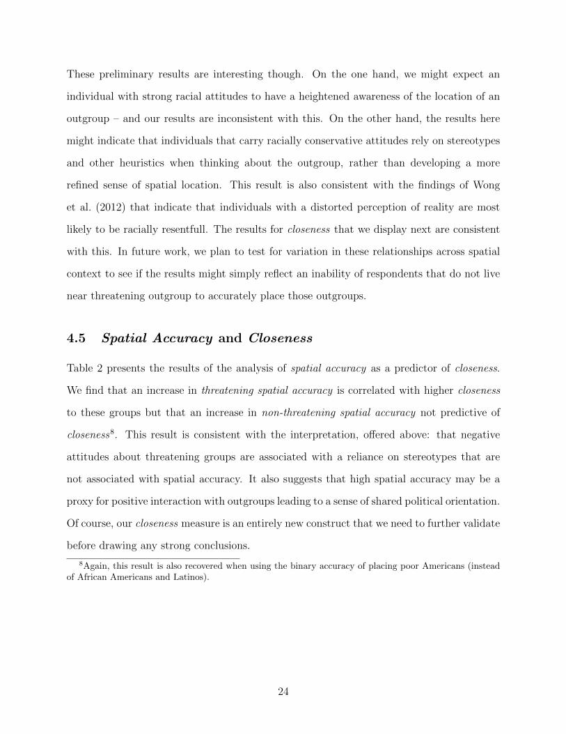
These preliminary results are interesting though. On the one hand, we might expect an
individual with strong racial attitudes to have a heightened awareness of the location of an
outgroup – and our results are inconsistent with this. On the other hand, the results here
might indicate that individuals that carry racially conservative attitudes rely on stereotypes
and other heuristics when thinking about the outgroup, rather than developing a more
refined sense of spatial location. This result is also consistent with the findings of Wong
et al. (2012) that indicate that individuals with a distorted perception of reality are most
likely to be racially resentfull. The results for closeness that we display next are consistent
with this. In future work, we plan to test for variation in these relationships across spatial
context to see if the results might simply reflect an inability of respondents that do not live
near threatening outgroup to accurately place those outgroups.
4.5 Spatial Accuracy and Closeness
Table 2 presents the results of the analysis of spatial accuracy as a predictor of closeness.
We find that an increase in threatening spatial accuracy is correlated with higher closeness
to these groups but that an increase in non-threatening spatial accuracy not predictive of
closeness8. This result is consistent with the interpretation, offered above: that negative
attitudes about threatening groups are associated with a reliance on stereotypes that are
not associated with spatial accuracy. It also suggests that high spatial accuracy may be a
proxy for positive interaction with outgroups leading to a sense of shared political orientation.
Of course, our closeness measure is an entirely new construct that we need to further validate
before drawing any strong conclusions.
8Again, this result is also recovered when using the binary accuracy of placing poor Americans (insteadof African Americans and Latinos).
24

Table 2: spatial accuracy and closeness
non-threatening groups threatening groupsIntercept 0.79 0.72
(0.56) (0.55)spatial accuracy −0.01 0.11∗
(0.04) (0.04)partisanship 0.38∗ 0.39∗
(0.04) (0.04)education 0.00 0.00
(0.01) (0.01)population density −0.00 0.00
(0.01) (0.01)county % white −0.01 −0.01
(0.01) (0.01)county % Black −0.01 −0.00
(0.01) (0.01)county % Asian −0.00 −0.00
(0.01) (0.01)county % Latino −0.01 −0.01
(0.01) (0.01)N 552 543R2 0.18 0.19adj. R2 0.17 0.18Resid. sd 0.21 0.21
Cell entries are OLS regression coefficients with white survey respondents only. Dependent variable is political
closeness. Standard errors in parentheses. ∗ indicates significance at p < 0.05
4.6 Racial Resentment, Demographic Innumeracy, and Spatial
Accuracy
In this section we briefly consider the relationship between demographic innumeracy (Wong
et al. 2012), spatial accuracy, and racial resentment. Table 3 shows the results from this anal-
ysis. Innumeracy is a measure of the respondents over-estimate of % Black in US: A 1-unit
increase in this variable corresponds to a 10 percentage point overestimate of demographic
concentration of Blacks in the United States. Because the accuracy of non-threatening
groups was significantly related to attitudes above, we use the average accuracy of whites
and Asians again.
25
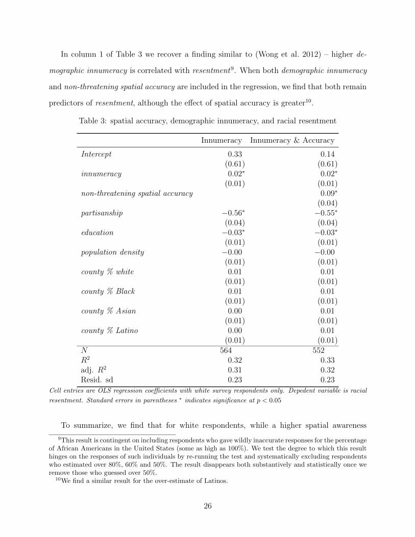
In column 1 of Table 3 we recover a finding similar to (Wong et al. 2012) – higher de-
mographic innumeracy is correlated with resentment9. When both demographic innumeracy
and non-threatening spatial accuracy are included in the regression, we find that both remain
predictors of resentment, although the effect of spatial accuracy is greater10.
Table 3: spatial accuracy, demographic innumeracy, and racial resentment
Innumeracy Innumeracy & Accuracy
Intercept 0.33 0.14(0.61) (0.61)
innumeracy 0.02∗ 0.02∗
(0.01) (0.01)non-threatening spatial accuracy 0.09∗
(0.04)partisanship −0.56∗ −0.55∗
(0.04) (0.04)education −0.03∗ −0.03∗
(0.01) (0.01)population density −0.00 −0.00
(0.01) (0.01)county % white 0.01 0.01
(0.01) (0.01)county % Black 0.01 0.01
(0.01) (0.01)county % Asian 0.00 0.01
(0.01) (0.01)county % Latino 0.00 0.01
(0.01) (0.01)N 564 552R2 0.32 0.33adj. R2 0.31 0.32Resid. sd 0.23 0.23
Cell entries are OLS regression coefficients with white survey respondents only. Depedent variable is racial
resentment. Standard errors in parentheses ∗ indicates significance at p < 0.05
To summarize, we find that for white respondents, while a higher spatial awareness
9This result is contingent on including respondents who gave wildly inaccurate responses for the percentageof African Americans in the United States (some as high as 100%). We test the degree to which this resulthinges on the responses of such individuals by re-running the test and systematically excluding respondentswho estimated over 80%, 60% and 50%. The result disappears both substantively and statistically once weremove those who guessed over 50%.
10We find a similar result for the over-estimate of Latinos.
26
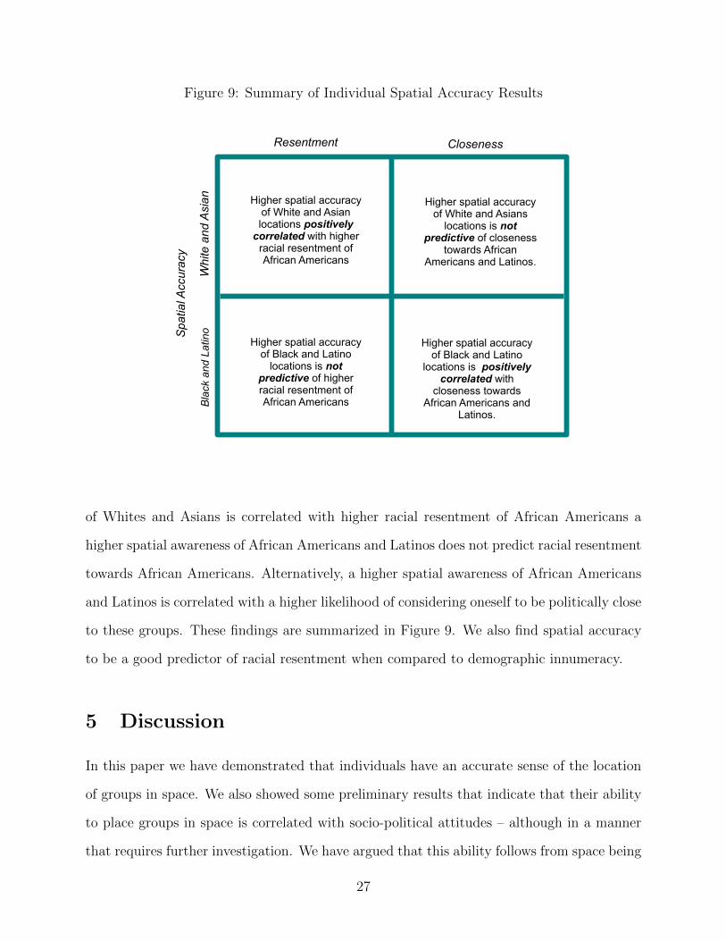
Figure 9: Summary of Individual Spatial Accuracy Results
Resentment Closeness
Whi
te a
nd
Asi
an
Bla
ck a
nd L
atin
o Higher spatial accuracy
of White and Asian locations positively
correlated with higher racial resentment of African Americans
Higher spatial accuracy of Black and Latino
locations is not predictive of higher racial resentment of African Americans
Higher spatial accuracy of Black and Latino
locations is positively correlated with
closeness towards African Americans and
Latinos.
Sp
atia
l Acc
urac
y
Higher spatial accuracy of White and Asians
locations is not predictive of closeness
towards African Americans and Latinos.
of Whites and Asians is correlated with higher racial resentment of African Americans a
higher spatial awareness of African Americans and Latinos does not predict racial resentment
towards African Americans. Alternatively, a higher spatial awareness of African Americans
and Latinos is correlated with a higher likelihood of considering oneself to be politically close
to these groups. These findings are summarized in Figure 9. We also find spatial accuracy
to be a good predictor of racial resentment when compared to demographic innumeracy.
5 Discussion
In this paper we have demonstrated that individuals have an accurate sense of the location
of groups in space. We also showed some preliminary results that indicate that their ability
to place groups in space is correlated with socio-political attitudes – although in a manner
that requires further investigation. We have argued that this ability follows from space being
27
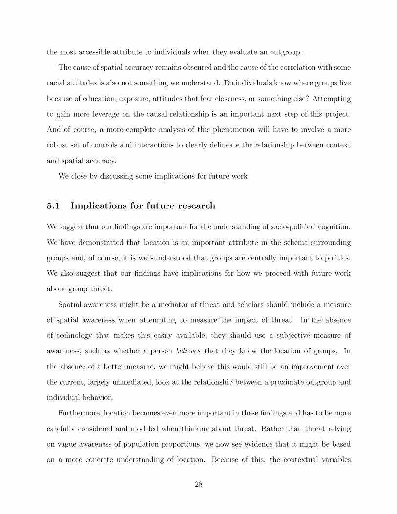
the most accessible attribute to individuals when they evaluate an outgroup.
The cause of spatial accuracy remains obscured and the cause of the correlation with some
racial attitudes is also not something we understand. Do individuals know where groups live
because of education, exposure, attitudes that fear closeness, or something else? Attempting
to gain more leverage on the causal relationship is an important next step of this project.
And of course, a more complete analysis of this phenomenon will have to involve a more
robust set of controls and interactions to clearly delineate the relationship between context
and spatial accuracy.
We close by discussing some implications for future work.
5.1 Implications for future research
We suggest that our findings are important for the understanding of socio-political cognition.
We have demonstrated that location is an important attribute in the schema surrounding
groups and, of course, it is well-understood that groups are centrally important to politics.
We also suggest that our findings have implications for how we proceed with future work
about group threat.
Spatial awareness might be a mediator of threat and scholars should include a measure
of spatial awareness when attempting to measure the impact of threat. In the absence
of technology that makes this easily available, they should use a subjective measure of
awareness, such as whether a person believes that they know the location of groups. In
the absence of a better measure, we might believe this would still be an improvement over
the current, largely unmediated, look at the relationship between a proximate outgroup and
individual behavior.
Furthermore, location becomes even more important in these findings and has to be more
carefully considered and modeled when thinking about threat. Rather than threat relying
on vague awareness of population proportions, we now see evidence that it might be based
on a more concrete understanding of location. Because of this, the contextual variables
28
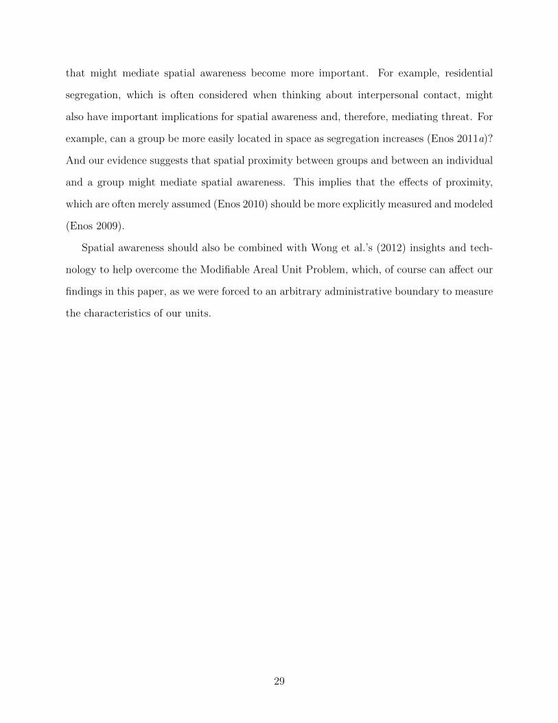
that might mediate spatial awareness become more important. For example, residential
segregation, which is often considered when thinking about interpersonal contact, might
also have important implications for spatial awareness and, therefore, mediating threat. For
example, can a group be more easily located in space as segregation increases (Enos 2011a)?
And our evidence suggests that spatial proximity between groups and between an individual
and a group might mediate spatial awareness. This implies that the effects of proximity,
which are often merely assumed (Enos 2010) should be more explicitly measured and modeled
(Enos 2009).
Spatial awareness should also be combined with Wong et al.’s (2012) insights and tech-
nology to help overcome the Modifiable Areal Unit Problem, which, of course can affect our
findings in this paper, as we were forced to an arbitrary administrative boundary to measure
the characteristics of our units.
29
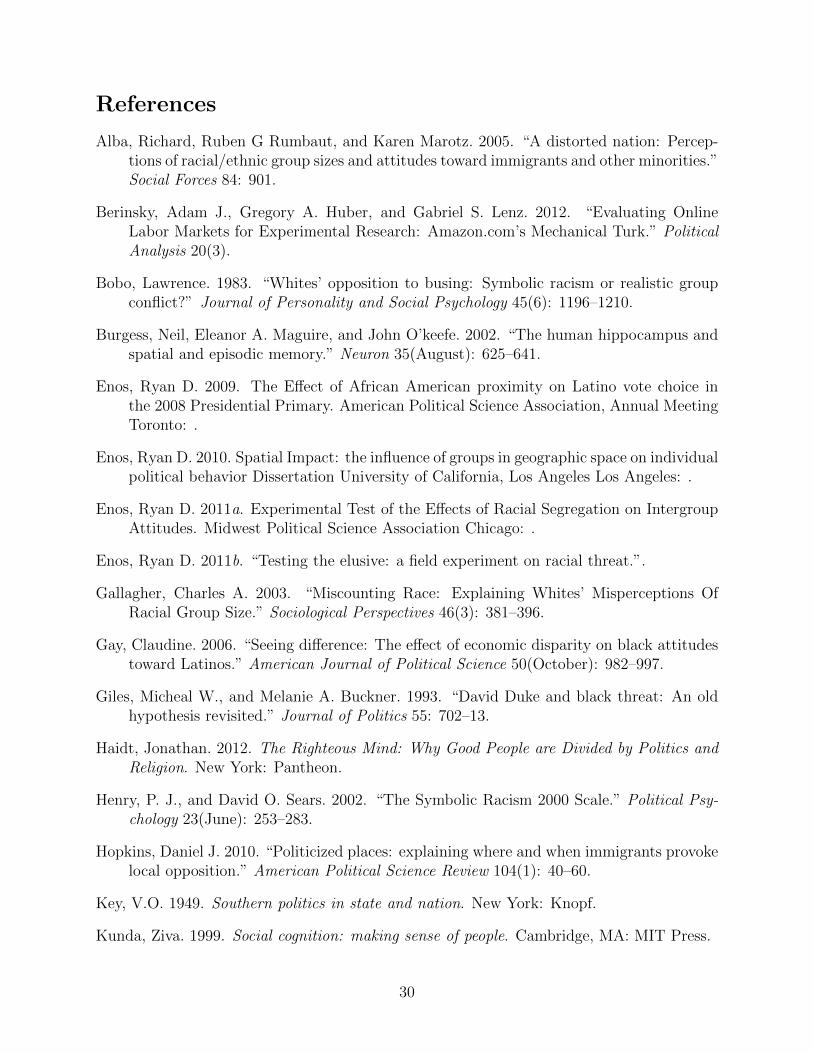
References
Alba, Richard, Ruben G Rumbaut, and Karen Marotz. 2005. “A distorted nation: Percep-tions of racial/ethnic group sizes and attitudes toward immigrants and other minorities.”Social Forces 84: 901.
Berinsky, Adam J., Gregory A. Huber, and Gabriel S. Lenz. 2012. “Evaluating OnlineLabor Markets for Experimental Research: Amazon.com’s Mechanical Turk.” PoliticalAnalysis 20(3).
Bobo, Lawrence. 1983. “Whites’ opposition to busing: Symbolic racism or realistic groupconflict?” Journal of Personality and Social Psychology 45(6): 1196–1210.
Burgess, Neil, Eleanor A. Maguire, and John O’keefe. 2002. “The human hippocampus andspatial and episodic memory.” Neuron 35(August): 625–641.
Enos, Ryan D. 2009. The Effect of African American proximity on Latino vote choice inthe 2008 Presidential Primary. American Political Science Association, Annual MeetingToronto: .
Enos, Ryan D. 2010. Spatial Impact: the influence of groups in geographic space on individualpolitical behavior Dissertation University of California, Los Angeles Los Angeles: .
Enos, Ryan D. 2011a. Experimental Test of the Effects of Racial Segregation on IntergroupAttitudes. Midwest Political Science Association Chicago: .
Enos, Ryan D. 2011b. “Testing the elusive: a field experiment on racial threat.”.
Gallagher, Charles A. 2003. “Miscounting Race: Explaining Whites’ Misperceptions OfRacial Group Size.” Sociological Perspectives 46(3): 381–396.
Gay, Claudine. 2006. “Seeing difference: The effect of economic disparity on black attitudestoward Latinos.” American Journal of Political Science 50(October): 982–997.
Giles, Micheal W., and Melanie A. Buckner. 1993. “David Duke and black threat: An oldhypothesis revisited.” Journal of Politics 55: 702–13.
Haidt, Jonathan. 2012. The Righteous Mind: Why Good People are Divided by Politics andReligion. New York: Pantheon.
Henry, P. J., and David O. Sears. 2002. “The Symbolic Racism 2000 Scale.” Political Psy-chology 23(June): 253–283.
Hopkins, Daniel J. 2010. “Politicized places: explaining where and when immigrants provokelocal opposition.” American Political Science Review 104(1): 40–60.
Key, V.O. 1949. Southern politics in state and nation. New York: Knopf.
Kunda, Ziva. 1999. Social cognition: making sense of people. Cambridge, MA: MIT Press.
30
Maguire, Eleanor A. 2006. Neuroergonomics - The brain at work. Oxford University Presschapter Spatial Navigation, pp. 131–135.
Martinez, Michael D., Kenneth D. Wald, and Stephen C. Craig. 2008. “Homophobic in-numeracy?: Estimating the size of the gay and lesbian population.” Public OpinionQuarterly 72(4): 753–767.
Milgim, Stanley. 1970. “The Experience of Living in Cities.” Science 167(March): 1461–1468.
Nadeau, Richard, Richard G. Niemi, and Jeffrey Levine. 1993. “Innumeracy about minoritypopulations.” Public Opinion Quarterly 57(3): 332–347.
Sigelman, Lee, and Richard G. Niemi. 2001. “Innumeracy about Minority Populations:African Americans and Whites Compared.” The Public Opinion Quarterly 65(1): 86–94.
Spence, Lester K., and Harwood McClerking. 2010. “Context, Black Empowerment, andAfrican American Political Participation.” American Politics Research 38(5): 909–930.
Voss, D. Stephen. 1996. “Beyond racial threat: Failure of an old hypothesis in the newSouth.” The Journal of Politics 58(4): 1156–70.
Wong, Cara. 2010. Boundaries of Obligation in American Politics: Geographic, National,and Racial Communities. New York: Cambridge University Press.
Wong, Cara J. 2007. ““Little” and “big” pictures in our heads: Race, local context, and innu-meracy about racial groups in the United States.” Public Opinion Quarterly 71(Septem-ber): 392–412.
Wong, Cara, Jake Bowers, Tarah Williams, and Katherine Drake. 2012. “Bringing the PersonBack In: Boundaries, Perceptions, and the Measurement of Racial Context.” Journalof Politics .
31