marc cowling, elisa ughetto, neil lee the innovation debt
TRANSCRIPT

Marc Cowling, Elisa Ughetto, Neil Lee
The innovation debt penalty: cost of debt, loan default, and the effects of a public loan guarantee on high-tech firms Article (Published version) (Refereed)
Original citation: Cowling, Marc and Ughetto, Elisa and Lee, Neil (2017) The innovation debt penalty: cost of debt, loan default, and the effects of a public loan guarantee on high-tech firms. Technological Forecasting and Social Change. ISSN 0040-1625 DOI: 10.1016/j.techfore.2017.06.016 Reuse of this item is permitted through licensing under the Creative Commons:
© 2017 Elsevier Inc. CC BY-NC-ND 4.0 This version available at: http://eprints.lse.ac.uk/81337/ Available in LSE Research Online: July 2017
LSE has developed LSE Research Online so that users may access research output of the School. Copyright © and Moral Rights for the papers on this site are retained by the individual authors and/or other copyright owners. You may freely distribute the URL (http://eprints.lse.ac.uk) of the LSE Research Online website.

1
The innovation debt penalty:
Cost of debt, loan default, and the effects of a public loan guarantee on high-tech
firms
Marc Cowling*, Elisa Ughetto**, Neil Lee***,
*University of Brighton, Brighton Business School email: [email protected] **Politecnico di Torino, Department of Management and Production Engineering, 10129 Torino, Italy Bureau of Research on Innovation, Complexity and Knowledge, Collegio Carlo Alberto, 10024 Moncalieri, Italy. email: [email protected] ***London School of Economics and Political Science email: [email protected]
Abstract
High-technology firms per se are perceived to be more risky than other, more conventional, firms. It
follows that financial institutions will take this into account when designing loan contracts, and that this
will manifest itself in more costly debt. In this paper we empirically test whether the provision of a
government loan guarantee fundamentally changes the way lenders price debt to high-tech firms.
Further, we also examine whether there are differential loan price effects of a public guarantee
depending on the nature of the firms themselves and the nature of the economic and innovation
environment that surrounds them. Using a large UK dataset of 29,266 guarantee backed loans we find
that there is a high-tech risk premium which is justified by higher default, but, in general, that this
premium is altered significantly when a public guarantee is provided for all firms. Further, all these loan
price effects differ on precise spatial economic and innovation attributes.
Keywords: cost of debt, high-tech firms, public loan guarantee scheme, loan default
JEL CODE: G21, G28
2
1. Introduction
Whilst there are clear economic benefits from innovation and technological advancement
(Laeven et al., 2015), innovation processes are highly uncertain in their outcomes (Jalonen, 2012;
Scherer et al., 2001). This means that financiers will view funding projects associated with these efforts
with caution. As small firms in general face a penalty due to their smallness per se, associated with the
relatively high fixed costs of lending (and of providing equity) and asymmetric information problems,
being innovative and technologically driven adds a further layer of asymmetry and informational
opacity (Carpenter and Petersen, 2002; Guiso, 1998; Hall, 2002; Himmelberg and Petersen, 1994;
Ughetto, 2008). In short, the literature predicts that in debt markets, smaller firms already face general
access problems and pay a premium on borrowing – but these problems may be worse for high-
technology firms (Berger et al., 2007; Hall and Lerner, 2010).
Whilst governments have intervened in this small business finance space explicitly to correct for
perceived market failures, or gaps in provision, in many ways, including loan guarantee schemes
(Cowling, 2010; Honohan, 2010; Ughetto et al., 2017), R&D tax credits (Cowling, 2016), grants, soft
loans, hybrid equity schemes (Aernoudt, 2005; Cannone and Ughetto, 2014), and business angel
schemes (Ramadani, 2009), the general approach to the financing of innovative and technology based
firms has favored equity funding and intervention in equity capital markets (Kortum and Lerner, 2000;
Langeland, 2007). This has largely ignored the potential role that debt (Kerr and Nanda, 2014) and
particularly loan guarantees might play in the funding of technology based firms. This is interesting in
itself as the purpose of a public loan guarantee is to reduce the (default) risk to the lender of providing
a loan to an informationally opaque smaller business (Honohan, 2010). In fact, the numerous loan
guarantee programs introduced around the world have been conceived to allow lenders to share with
the government the risk of default on outstanding loans, with the latter partially or totally covering any
potential loss (Beck et al., 2010; Boschi et al., 2014; Cowling and Mitchell, 2003; Honohan, 2010).
These public guarantee instruments, although differing in their characterizing features across nations
(i.e. percentage of guaranteed coverage, lending criteria, industry and geographical limitations, loss

3
distribution policy), share the common aim of reducing the barriers to additional finance for borrowers
that mostly suffer from credit constraints (Cowling and Siepel, 2013)1.
To the best of our knowledge no empirical works have investigated, in the context of publicly
guaranteed schemes, the dynamics of loan pricing and loan default when borrowers are high-tech firms.
In particular, we are not aware of any study examining to what extent small high-tech firms face higher
default rates and a greater cost premium for the use of debt finance compared to their non high-tech
peers when lending is guaranteed by government. On the one side, it is expected that banks charge a
higher cost of capital to high-tech firms because of their higher risk, uncertain returns, and lack of
collateral assets. On the other hand, the presence of the public guarantee should somehow attenuate
such “innovation debt penalty”. The paper adds to extant literature in two respects. First, it is the first
study to investigate whether the presence of a government backed loan guarantee alters banks view in
respect of the loan risk-premium charged to high-tech firms. Second, it differentiates from previous
works in the field because it questions whether there is any spatial variation in both the cost of loans to
high-technology firms and in their default rates.
In this paper we explore several key aspects of lending to technology based smaller businesses,
using a large UK dataset of 29,266 loans issued under the Small Firm Loan Guarantee (SFLG) public
Scheme. The scheme, established in 1981 by the UK Government, targets young and small businesses
(up to five years old and with an annual turnover of up to £5.6 million) that lack track records or
collateral to secure loans and has been conceived in eight distinct phases.
Our analysis, which concentrates on the phases VI and VII of the Scheme (2000-2005), is
twofold. Firstly, we quantify whether high-tech firms have a higher default risk than more conventional
firms, and whether they face a double-hurdle of being small and being innovative in respect of the price
premium they pay on their borrowing, when lending is guaranteed by government (Lee et al., 2015).
1
However, it has been found that the “credit additionality” effect induced by such schemes may not be achieved when the government coverage falls below a certain threshold (Boschi et al., 2014).

4
Indeed, we test the presence of a differential effect in terms of the loan price charged by banks for
high-tech firms compared to their more conventional small firm peers. Secondly, we are able to trace
out more nuanced loan price effects relating to the specific loan contract terms, the spatial location of
the firms and the competitive, innovative and economic environment that surrounds them. In doing so
we hope to build upon a growing body of research that has begun to unravel some key questions
relating to innovation financing in the context of public loan guarantee programmes (see Cincero and
Santos, 2015).
The rest of the paper is set out as follows. Firstly, we review the literature in several related
areas including small firm and high-technology firm financing, also in the context of guaranteed
lending, and the effects of economic geography on the financing outcomes of smaller firms. Secondly,
we discuss the empirical data and present the basic sample descriptive statistics. We then present our
empirical modelling of the loan spread (our measure of the price of lending) and of loan default (our
measure of loan riskiness) under the UK policy intervention scheme. We conclude by summarizing our
findings and setting this in the context of previous literature. Public policy impacts and implications are
also discussed given the centrality of publicly supported loan guarantee schemes in the small business
finance arena.
2. Literature review
2.1 The financing of high-technology firms
There are longstanding concerns that high-technology or innovative firms may find themselves
credit constrained (Revest and Sapio, 2010; Ughetto, 2008; Westhead and Storey, 1997). Work in this
area has focused on several explanations. The most important is asymmetric information (Burgstaller,
2013). In the classic explanation of credit constraints for small firms, Stiglitz and Weiss (1981) argued
that information asymmetries may cause adverse selection in credit markets making it rational for
borrowers to restrict lending to certain types of firms, rather than raising the price of loans. In a similar

5
manner to the classic ‘market for lemons’ (Akerlof, 1970), higher loan costs drive out the better quality
applicants, lowering average quality and leading lenders to restrict financing. For innovative firms, this
problem of asymmetric information is mitigated by patenting, which provides an indicator of the
quality of innovation to the lender and so reduces loan spreads (Francis et al., 2012; Plumlee et al.,
2015).
Yet three additional factors might make it costlier to lend to innovative firms and so raise bank
margins. The first is that the expected future revenues arising from investments in scientific and
technological research are uncertain. Secondly, an evaluation of the quality and strength of intellectual
property rights is expensive and often requires specialist expertise, thus adding to the per unit cost of
lending. To some degree, the second is the related challenge of raising collateral. Intangible assets such
as new products are hard to value and so difficult to use as collateral (Mina et al., 2013). The third is the
reluctance of innovative firms to reveal information to the market for valuation and so forced to rely
on internal finance (Magri, 2009). These factors raise screening costs for lenders, making it hard to
overcome the information problems identified by Stiglitz and Weiss (1981).
A second explanation is the idiosyncratic nature of risk in the development of new, innovative
products (Mina et al., 2013). By their nature, investments in R&D, new products or processes are risky
activities – while some such investments will pay off, the majority yield relatively little return (Carpenter
and Petersen, 2002; Coad and Rao, 2008; Hall, 2002). Moreover, high-technology firms may be seeking
finance for R&D which is more speculative still (Westhead and Storey, 1997). While funders taking
equity stakes may be interested in the long-term value of the company, banks are principally interested
in the simple ability of lenders to repay and benefit little beyond the repayment of a loan if a product is
highly successful.
Empirical work has shown a strong link between banking and technological progress. For
example, Amore et al. (2013) show that the deregulation and greater banking competition is associated
with increased innovation. Similarly, Hsu et al. (2015) use patenting data to show that firms which have

6
a strong patent portfolio pay lower spreads. However, these studies tend to focus on patenting – an
output measure of innovation, which reflects investments in research and development (R&D) which
have already been made. In contrast, firm level studies considering firms involved in regular innovative
activity often show that innovative firms are more credit constrained. Both Freel (2007) and Lee et al.
(2015) find that innovative small firms are more likely to be rejected when applying for bank loans. The
precise indicator of innovation seems to matter. But while several studies have considered alternative
types of innovation, relatively few studies have considered high-technology firms explicitly. This is
important as the link between the firm and the industry is more closely aligned in respect of high-
technology, and this in turn more closely maps into the way banks make lending allocation decisions.
While the categorization of firms into high-tech and low-tech may cast some firm-level heterogeneity in
innovation and R&D propensities, it has been established that banks make annual strategic lending
choices at the industry sector level in terms of their broad allocation of credit (see Cowling, 2010 for
the UK context). Capital in this sense flows to industries, not firms per se.
2.2 Geographical context and financing high-technology firms
Despite this evidence base, relatively fewer studies have considered regional variation in these
patterns of financing. However, there is increasing interest in the idea that regional factors, such as the
level of banking development or innovation intensity may matter for firm financing (Crocco et al.,
2012; Munari and Toschi, 2015). Studies on IPO’s, for example, suggest that underpricing is more likely
the further the firm is located from the financial capital (Acconcia et al., 2011). This is an important
question, as the availability of firms to access finance is seen as an important determinant of subsequent
economic growth – with empirical evidence suggesting finance is particularly important in deprived
regions (Craig et al., 2008).
One theoretical position in this area is that distance between providers of finance and potential
borrowers may hinder exchanges of information and make it harder for firms to access the finance they
need (Ughetto, 2009). With regard to equity finance, the classic Silicon Valley venture capitalists are

7
stereotypically imagined to follow a ‘2 hour rule’ where they are unwilling to make investments beyond
from their headquarters because doing so increases the cost of monitoring investments. Empirical work
does support the idea of local bias in venture capital investments, although this is particularly the case
for younger VCs (Cumming and Dai, 2010).
Building on a similar institutional framework, equity stakes are seen as being geographically
limited, meaning that firms in ‘core regions’ find it easier to access finance than those in peripheral
areas. Essentially, the clustering of investment activity in particular cities and regions may create a self-
reinforcing bias towards these areas, with both investment opportunities and specialist investors
clustering in technologically advanced regions. These ‘thick-markets’ for specialist finance will be
reflected in both the demand and supply of finance. Yet, this might mean that the relatively few
investment opportunities which arise in relatively low-tech regions are actually a higher quality. In their
study of VC investments in the US, Chen et al. (2010) show investments made outside of the core
regions are rarer but, because they have to be higher quality, more profitable on average.
While there is good evidence on the link between information and equity investments, fewer
studies have considered the relationship between banks and the geography of innovative firms finance
(Lee and Brown, 2016). One approach to explaining why banks may be less likely to lend to innovative
firms in particular regions lies in the distinction between soft information, non-codified information
about the firm which is hard to transmit electronically and is often developed through face to face
contact, and hard information, such as credit records or company accounts, which can easily be
transmitted from place to place. A simple explanation for regional variation in the financing of high
technology firms is that persuading finance providers of the merits of innovative high-technology
projects may require soft information, and this soft information may be locally bound. Banks focusing
on high-technology industries may focus more on soft rather than hard information in their lending
decisions. For example, Brown et al. (2012) show that banks do not use credit rating information to the
same degree when evaluating lending applications from high-technology firms, although high-tech
firms still face greater difficulties in accessing finance than low-tech firms.

8
There are several grounds for criticism of this approach. In the first place, the distinction
between soft and hard information may not be as simple and clear-cut as portrayed (Wojcik, 2011). But
it may also be that the structure of the banking sector in particular regions is more important than
simple distance. For example, Alessandrini et al. (2009) suggest that the more hierarchical levels there
are in a bank, the harder it will be to exchange soft information, and so this functional distance would
matter for innovation as much as actual geographical distance. They show that firms in Italian regions
where the banking system is functionally distant are less likely to introduce new innovations, with firms
further from core banking centres financially constrained. In contrast, the regional share of big banks
did not seem to matter. Similar evidence is presented for Austrian districts by Burgstaller (2013) who
finds that higher bank competition is associated with lower margins, although the author does not
focus on high-technology firms specifically.
A second set of potential explanations focus on the development of specialist spatial industries
and markets to serve the investment and general financing requirements of high-tech firms. Classic
explanations of innovation ecosystems show inter-related sets of financiers, entrepreneurs and other
institutions developing together. However, in regions with few innovative firms’ these synergies may
not operate and thin-markets for specialist finance may develop as increased search costs make it
uneconomic for providers to operate (Nightingale et al., 2009). Reflecting this, Chen et al. (2010) show
that venture capitalists in the United States tend to invest in areas where past investments have been
successful, and that the most successful investment firms tend also to be located in these core areas.
The corollary of this is that banks in regions with high shares of tech firms may develop specialist
lending facilities, such as those offered by banks in high-technology clusters such as Tech City. This
might mean that the share of high-technology firms in a region is associated with a reduced cost of
borrowing, as banks become better at screening borrowers.
Similarly, others have been concerned about the relationships with regional development.
Financing of high-technology firms has a two-directional relationship with regional development, with
availability of finance both a cause and a consequence of regional growth. While some studies have

9
considered this in the UK case, the evidence is mixed. Westhead and Storey (1997) show no evidence
that high-technology firms in assisted areas (deprived regions) of Britain are more likely to be
financially constrained. In contrast, Lee and Brown (2016) show that innovative companies in less
affluent UK areas are particularly likely to report rejection rates.
2.3 Loan Guarantee Schemes
Governments in more than one hundred countries across the developed and developing world
operate loan guarantee schemes (often called partial credit guarantee schemes, PCGs) (Beck et al.,
2010). The pervasiveness of loan guarantee schemes as a primary instrument to promote SME lending
implicitly assumes that there is a market failure in the provision of debt finance to SMEs, and, that by
altering the risk-return payoff for private banks, private banks will increase their willingness to lend to
informationally opaque and/or asset poor SMEs with viable funding proposals (Cowling, 2010;
Cowling and Siepel, 2013; Honaghan, 2008). The key parameter in terms of changing the banks risk-
return function is the coverage ratio, the proportion of the loan advanced by the private bank
guaranteed by the government in the event of borrower default (Beck et al., 2010). Across the seventy
six guarantee schemes covered in the 2008 World Bank review, the median coverage (guarantee) ratio
was 80%. A later World Bank study of MENA countries (Saadani et al., 2011) found a slightly lower
median guarantee of 75%. The guarantee level ensures that part of the lending risk is shared by the
bank thus increasing their incentives to properly conduct due diligence at the point of loan application
and to monitor successful loan applications, both of which act to reduce expected losses arising from
loan default.
The outcome evidence base is growing, but not as complete as would be required to make a
comprehensive judgement on the generalizable efficacy of loan guarantee programmes as a policy
instrument. Context is clearly important and the specific nature of spatial capital markets and scheme
parameters have a decisive impact on the outcomes achieved. The first issue we concern ourselves with
is finance additionality, or in North America incrementality. Evidence from the UK schemes found that

10
scheme additionality was increasing over time as the target groups became more focused and lending
banks were subject to greater scrutiny. The 1999 UK evaluation (KPMG, 1999) estimated that 70% of
loans were additional in that firms could not have accessed any market based debt finance. This
increased to 79% in the 2010 UK evaluation (Cowling, 2010), and 82% in the 2013 UK evaluation
(Allinson et al., 2013). Comparable estimates for the Canadian scheme (Riding et al., 2007) reported a
figure of 74.8% additionality. On job creation, the evidence that guarantee schemes can be associated
with net job creation is fairly strong. For the US, Brown and Earle (2016) find that the net cost per job
created over two decades was US$ 21,000 – 25,000, and that these effects were stronger for younger
firms and when local credit conditions are weak. UK evidence found that net jobs cost averaged £5,500
- £10,000 per job created (Cowling, 2010) and that on average each supported firm created 0.4 jobs per
annum, which was smaller than the later evaluation which reported 0.96 net jobs per firm per annum
(Allinson et al., 2013). Both French (Lelarge et al., 2010) and Norwegian evidence (Poyry, Damwad,
Agenda Kampang, 2010) also supported the job creation success of guarantee schemes. On loan
default, UK estimates report 3 year loan default figures of 33.3% for SFLG and 28.0% for Enterprise
Finance Guarantee (EFG), the newer scheme. The French scheme increased default by 6.2 percentage
points compared to normal lending, and estimates for the Italian scheme suggest a 2.5% increase in
default. But, importantly, the costs of default were not proportional to the actual default rate. UK
estimates show that default cost was only 17.2% of total loan value which implies a net cost per
recipient of only £5,000.
3. Dataset and descriptive statistics
The data we used in this study include the loans issued under the UK SFLG public loan
guarantee scheme over the period 2000 to 2005 and were provided by the UK Department for
Business Innovation and Skills (DBIS). Other works have previously exploited the dataset in its
previous releases (see Cowling and Mitchell, 2003 and Cowling, 2010) and in its current form (see

11
Cowling and Siepel, 2013 and Ughetto et al., 2017). The initial dataset includes 31,434 guarantee backed
loans issued between 2000 and 2005 by 25 financial institutions in the UK (of which 80% are issued by
Barclays Bank Plc, National Westminster Bank plc, Lloyds Bank plc, HSBC Bank Plc, i.e. the four
major UK banks).
After we dropped observations reporting missing values and outliers in the main computed
variables, we ended up with a final sample consisting of 29,266 SFLG backed loans. To identify high-
tech firms we searched the 4 digit SIC codes for each firm and applied the Eurostat classification based
on Rev. 2 NACE 2-digit level codes to the corresponding SIC codes. Similarly to other previous works
(e.g. Benfratello et al., 2008; Himmelberg and Petersen, 1994; Ughetto, 2008; Ughetto et al. 2017), high-
tech firms are those operating in the following manufacturing sectors: computer, electronic and optical
products; chemicals and drugs; electrical equipment; mechanical machinery; transportation equipment2.
To test the differential impact on the cost of debt and on the probability of default that loans
issued to high-tech firms might have when different regional conditions apply, we searched for
economic data on UK regions. The UK Competitiveness Index (year 2005), provided by the Centre for
International Competitiveness, was used to distinguish between developed and lagging regions3. To
measure the level of financial development of the local credit markets, we collected data on the regions’
number of bank branches from Eurostat-Regio (year 2003) and constructed a measure of bank branch
density (number of branches divided by population), as it was done in previous studies (see, for
instance, Benfratello et al., 2008; Ughetto et al., 2017). Financially developed regions have been defined
as regions with a bank branch density higher than the median. Data on the total number of firms in the
different SIC sectors in UK regions were extracted from the Office of National Statistics (2005). We
then applied the Eurostat classification on High-tech industry to identify high-tech sectors and
calculated the number of firms in the high-tech sector (as a percentage of total firm population) for
2 http://ec.europa.eu/eurostat/cache/metadata/Annexes/htec_esms_an3.pdf
3 Such index is a composite indicator based on: 1) input factors (i.e. R&D expenditure, economic activity rates, business
start-up rates per 1,000 inhabitants, number of businesses per 1,000 inhabitants, proportion of working age population with NVQ level 4 or higher, proportion of knowledge based businesses), (2) output factors (i.e. value added per head at current basic prices, exports per head of population, imports per head of population, productivity-output per hour worked, employment rates) and (3) outcome factors (gross weekly pay, unemployment rates).

12
each UK region to define technologically advanced regions. We also collected from Eurostat-Regio
data on labour cost, wages and salaries and direct remuneration per hour per employee and number of
firms younger than 3 years (as a percentage of total firm population) to identify high labor cost regions
and young firm regions.
In our empirical analysis we employ two dependent variables in the IV OLS and probit models
respectively: (1) the spread, our measure of the price of lending, defined as the bank margin over base
deflated by price index, and (2) the default, a dummy variable equal to 1 if the loan defaults and 0
otherwise. Spreads are on average around 3.12%, although they can peak at much larger values. Out of
29,266 loans issued, nearly 28% ended in default. The typical firm in our sample receives a loan of the
average amount of £63,937 (but loans can reach higher amounts up to £250,000). Guarantee backed
loans are issued mainly to cover working capital needs (56.5%). Descriptive statistics show that more
than half of the firms’ total amount of financial debt is covered by the public guarantee (58%), although
this percentage can rise up to a maximum of 85%. It has to be noted that the share of publicly
guaranteed debt is fixed and determined by the policy scheme (in Phase VI, the Government coverage
is 70% of the loan amount for firms with less than two years and 85% for older borrowers and in Phase
VII it is 75%), so that the variation of the “guarantee coverage” is driven by the relative incidence of
the guaranteed loan with respect to the amount of the other financial debt.4
We also know that firms have overdraft facility outstanding in 37.1% of the cases. Firms
applying for a guarantee backed loan are mostly micro and small-sized enterprises, reporting an average
turnover of £0.35 million. High-tech firms represent the 10.4% of the sample. 59.8% of the firms are
located in financially developed regions, 40.8% in developed regions, 41.4% in technologically
advanced regions, 45.4% in high labour cost regions and 49.6% in young firm regions.
4
In fact, the variable “guarantee coverage” is defined as the ratio between the amount of the loan covered by the public guarantee and the total amount of outstanding loans (included the amount of financial debt, provided by any eligible bank in the UK, that a firm has in addition to the guarantee-backed debt). This variable is influenced by the interplay of the policy initiative and the previous demand/supply for banks loans, which might reflect unobservable firm-level factors.
13
A listing of the variables used in the empirical analysis along with their definitions and their
descriptive statistics (mean, median, standard deviation) is provided in Table 1.
[Insert Table 1 here]
4. Empirical analysis
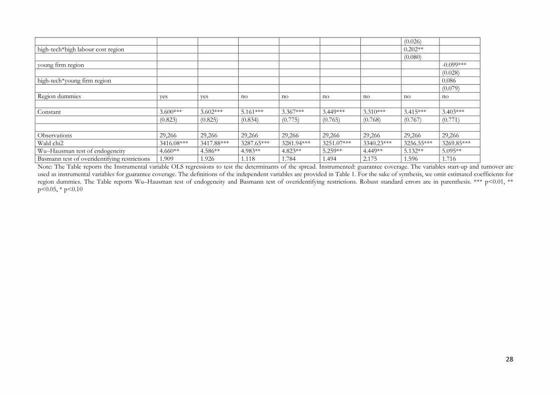
In this section we first present a set of Instrumental variable (IV) OLS regressions (Table 2) in
which the dependent variable is the spread (the adjusted loan interest rate). Instrumental variable
regressions allow us to control for potential endogeneity problems (Wooldridge, 2002). The
endogeneity problems attain the variable guarantee coverage, which might be affected, as it happens for
the loan spread, by firm riskiness and other unobservable exogenous shocks. The variables start-up and
turnover are used as instrumental variables for guarantee coverage. Table 2 reports the Wu–Hausman
test for endogeneity. The null hypothesis is that guarantee coverage can be treated as exogenous. The
Wu–Hausman test statistics are significant in all model specifications, suggesting a rejection of the null
of exogeneity. The choice of these two instrumental variables is supported by the Basmann test of
overidentifying restrictions5.
A more comprehensive picture of the determinants of the spread can be obtained by using
quantile regressions (reported in the Appendix). While OLS regression focuses on the mean of the
dependent variable, quantile regressions model the relationship between a set of regressors and the
percentiles (Koenker and Bassett, 1978; Mosteller and Tukey, 1977). In our specific case, the quantile
regression estimates the change in a specified quantile of the spread produced by a one unit change in
an explanatory variable. This allows us to compare how some percentiles of the spread distribution may
5 The exogeneity condition implies that at least one instrument must be exogenous. The exogeneity of the instrument “start-
up” can be justified from a theoretical point of view, referring to the specific context of the SFLG scheme. Indeed, the variable start-up is negatively correlated with the variable guarantee coverage because start-ups do not usually have previous debt, but is unrelated to the outcome (spread). This is possible because the SFLG Scheme is financing young firms aged between 0 and 5 years old. While it can be expected that firm age has a non negligible effect on the spread in a sample of firms characterized by a large variance of firm age, this is not the case with our specific sample. Indeed, it might be argued that in the specific SFLG Scheme context, interest rates are charged based upon other unobservable firm-related factors (e.g. such as the quality of the business plan).

14
be more affected by certain loan and firm characteristics more than other percentiles, a particular
concern because of the potentially skewed distribution of risk amongst high-technology firms. To
tackle the previously mentioned endogeneity problem, we run IV quantile regressions, using a relatively
new method and coding (i.e. ivqreg routine for Stata developed by Kwak, 2010). The variables start-up
and turnover are used as instrumental variables for guarantee coverage.
We then run a set of probit models to predict the probability of loan default (Table 3). High-tech is
our main variable of interest. The aim of the analysis is to study the loan pricing conditions and the
probability of loan default for high-tech applicants. We are also interested in identifying specific
differential patterns when high-tech firms are located in regions with different levels of economic,
financial and technological development and when different macro-economic conditions and types of
lenders apply. We therefore interact the dummy variable high-tech with a number of variables
identifying regional and economic dimensions. Independent variables include the amount of the loan
covered by the guarantee scheme as a percentage of the total amount of outstanding loans, firm and
loan characteristics. We also control for sectors, regions, banks and macro-economic conditions.
Table 2 reports the econometric analysis of the determinants of the spread through IV OLS
regressions. Model 1 illustrates the baseline specification that includes among the regressors a set of
basic loan (i.e. guaranteed coverage, loan amount, additional loan commitments, loan purpose) and firm
level variables (i.e. company status, high-tech). The main variable of interest for the purpose of the
study is whether firms belong to the high-tech sector. We control for region dummies and macro-
economic conditions (GDP growth). We then augment this specification by including interaction
variables equal to the dummy high-tech times dummy variables on whether the loan was granted by the
biggest four UK banks (model 2) and in recession times (model 3). The high-tech dummy variable is
then interacted with a number of variables identifying whether loan applicants are located in
economically and financially developed regions (models 4 and 5), technologically advanced regions
(model 6), high labor cost regions (model 7) and regions with a large population of young firms (model
8).

15
Results in Table 2 indicate that the higher is the incidence of the publicly guaranteed debt over the
total amount of outstanding loans, the lower is, on average, the spread6. Higher margins are charged for
loans issued for working capital purposes and in periods of economic growth. Higher rates are also
applied for limited partnerships/companies and by the biggest four UK banks, although this effect
loses statistical significance in models 5 and 7.
High-tech firms are charged, on average, higher rates on loans. This result is significant at 1%
level of statistical significance in all model specifications. This is in line with the expectation that high-
tech firms face a greater cost premium for the use of external finance because of their limited
availability of collateral to secure firms’ borrowing and the high degree of risk which characterizes the
returns of R&D investments.
We find evidence that the public loan guarantee scheme is successful in reducing the cost of
debt for firms located in economic and financially developed regions, technologically developed, high
labor costs and young firm regions. In these regions loan applicants are charged, on average, lower
spreads. It is in fact plausible that more creditworthy firms populate these areas because of the greater
opportunities they receive in terms of access to credit, infrastructures and business networks, leading
banks to apply lower margins on their loans. However, it is also the case that closer proximity to small
business customers lowers information asymmetries. In addition, there is the potential for financial
institutions in more developed financial markets to invest more in information processing systems to
support lending. Finally, there is a more textbook competition effect on prices in that greater
competition for loans from the supply side reduces prices in the market.
6 In a previous work (Ughetto et al., 2017), we investigated for which type of borrowers and loans does the public guarantee
generate a more favorable effect (in terms of reduction in the cost of capital). We found that an increase of the incidence of
the debt guaranteed by government with respect to the total outstanding debt leads to a contraction in the spread only for
loans covering working capital needs rather than investments. However, we did not find any differential impact when the
sample is split according to whether borrowers belong to high-tech or low-tech manufacturing sectors and to knowledge-
intensive or less knowledge-intensive service sectors.

16
From a public policy perspective, it is interesting to examine whether differential patterns on
the spread charged to high-tech firms differ by regional and economic context. We find positive and
significant coefficients for the interactions between the variable high-tech and the binary variables
identifying the regions characterized by high levels of labor cost (model 7) and economic development
(model 4) and technological advances (model 6). Hence, the impact on the spread for firms belonging
to the high-tech sector is larger if they are located in high labor cost, technologically advanced and
developed regions7. The interaction effect is not significant when high-tech firms receive their loans
from the biggest 4 UK banks and when they are located in financially developed regions or in regions
with a large population of young firms. Results also indicate that lower margins are applied in states of
a bad economy and that this holds true for high-tech firms.
[Insert Table 2 here]
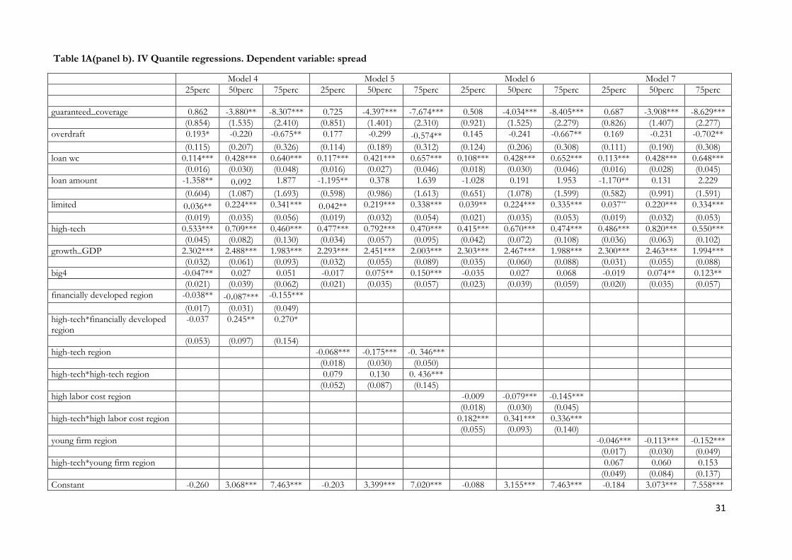
The IV quantile regression results in Table 1A show that the IV OLS estimates do not tell the
whole story. The value of the estimated coefficients for the variable high-tech seems to vary over the
spread distribution, with the highest coefficients at the median (50th percentile). When interactions are
considered, the negative association between the spread and the interaction variable high-
tech*recession is significant at both 25th and 50th percentiles, but it is not significant at the 75th
percentile. The impact on the spread for high-tech firms located in developed regions is larger for
higher percentiles of the spread (75th percentiles). A positive and significant correlation between the
spread and the interaction variable high-tech*high-tech region is only found at the 75th percentile. At all
percentiles the variable ‘high-tech * high labor cost region displays a positive and statistically significant
effect on the spread, showing a bigger effect in the 50th and 75th percentiles. The coefficients for loans
issued to cover working capital needs and for guaranteed coverage are larger at the 75th percentiles, and
the latter is not significant at the lowest quantiles.
7 We also experimented with alternative variables concerning the technological development of a region, such as if the firm
is located in a region with total R&D personnel in head count in percentage of active population greater than the sample median and in a region with employment in technology and knowledge intensive sectors greater than the sample median. Results are in line with those reported in Model 6 of Table 2.

17
In Table 3 we run a simple probit model on the probability that the loan ends in default.
Understanding what drives default and what is the probability that loans received by high-tech firms
end in default and how this varies when different time and local conditions apply is crucial for an
assessment of the cost to government of running the scheme. The default rate for the total population
of SFLG loans over the period 2000-2005 is 28% and this percentage rises to 36% for the sub-sample
of high-tech firms. The dependent variable of the probit model is default, which is a binary outcome
coded 1 if the loan ended in default and zero otherwise. Independent variables are the same reported in
previous IV OLS regressions.
We observe that firms with higher turnover show, on average, lower default rates. Loans used
for working capital purposes on average have higher default rates, and this effect is significant at 1%
level. The increase in the likelihood of default due to marginal increases in the variable loan wc is
approximately 9.8%. In contrast, no relationship is found between loan amount and default. The
relationship between the guarantee coverage and subsequent default is not statistically significant. As
expected, in recessionary times the probability of default is greater than in good states of the economy.
Interestingly, firms located in economically developed, technologically advanced and young firm
regions are more likely to default, while firms located in financially advanced regions are the least likely
to default.
The key finding from the default model is that there is a positive relationship between high-tech
applicants and subsequent default. This result is significant at 1% level and robust in almost all model
specifications (with the exception of model 7). Being a high-tech firm increases the default probability
by approximately 5%, depending on the considered model (from the lowest 3% to the highest 7%).
Interaction effects in the probit model show a negative and significant correlation with the default
probability for the interacted variables high-tech*big4, high-tech* developed region, high-tech* high-
tech region and high-tech*young firm region, while high-tech* financially developed region displays a
positive and significant correlation with the dependent variable. Looking at the magnitude of the

18
interaction effects8, it emerges that high-tech firms are 3.7% more likely to default if the loan is not
provided by the biggest four banks. Instead, loans provided to high-tech firms from one of the four
biggest UK banks have a comparatively lower probability to default (even if, on average, such loans are
associated with higher default rates). In fact, the probability of default decreases by 1.2% when high-
tech firms are financed by the major four UK banks. This effect is significant at 5% significance level.
For high tech firms belonging to financially developed regions the probability of default is 10.6%
higher, while firms not belonging to a financial developed region are 7.3% more likely to default (at 1%
level of statistical significance). It also emerges that high-tech firms operating in economically advanced
and young firm regions are 1.2% more likely to default, but this effect is not statistically significant. The
likelihood of default decreases by 0.8% for firms operating in high-tech regions but again this effect is
not statistically significant.
[Insert Table 3 here]
5. Conclusions
We have explored in depth several key questions relating to small business lending in the
context of high-technology firms under a prominent UK publicly guaranteed scheme. In particular, we
questioned; (a) whether high-technology firms are a greater lending risk, (b) whether technology firms
face an additional loan price premium over and above that relating to their smallness (the innovation
penalty), (c) whether the presence of a government backed loan guarantee alters banks view in respect
of their loan risk-premium, (d) whether spatial location of the firm in the context of the specific
regional economic, innovation, and competitive position alters the way banks price lending to
technology firms.
Firstly, we found clear evidence that high-technology firms present a higher default risk to
banks with loan default being observably higher than that of conventional firms. But the difference in
8
As pointed out by Ai and Norton (2003) the magnitude of the interaction effect in nonlinear models does not equal the
marginal effect of the interaction term.

19
predicted loan default probabilities for high-technology firms was not particularly large, suggesting that
they are not as risky as might be commonly perceived. In relation to the price of lending, our core
finding was that there is evidence of an ‘innovation premium’ on lending to high-technology firms. But
this was only in the region of 0.5-0.6% which suggests that the actual magnitude of the ‘innovation
premium’ is not particularly large in the presence of a substantial guarantee coverage rate. Further, it
was the case that the provision of the public loan guarantee lowered interest spreads significantly for all
firms.
In general, we found that banks penalize short-term lending, particularly for working capital.
This suggests that cash-flow problems and the inability to self-finance working capital from retained
earnings is viewed as a poor signal by lending banks. In periods of economic growth, banks also appear
to take advantage of firms relative lack of price sensitivity and charge higher loan rates. In line with
what standard economic models of imperfect markets predict, the big-4 UK banks lend at higher rates
than their smaller counterparts. When combined with their ability to raise cheap capital on international
markets, and their ability to extract surplus profits from non-lending related activities from customer
firms, small firm lending for bigger banks is likely to be substantially more profitable.
We found evidence of spatial variation in both the cost of loans to high-technology firms and
their default rates, although our evidence is relatively nuanced. At a general level, lending is cheaper in
economically developed regions, in regions with highly developed financial markets, in regions where
there is a significant high-technology cluster and presence, and in regions characterized by a young and
dynamic business sector. But these benefits are not shared equally across all firms. In particular, high-
tech firms still face a debt penalty in economically developed regions, in technologically advanced
regions and in high wage (labor cost) regions. This might suggest that when banks have a large demand
for loans from conventional, lower-risk, firms, then the need to expand their lending to high-tech firms
incurs a penalty, even when the regional economy is buoyant and technologically fervent.

20
However, it was also interesting to note that high-tech firms faced no penalty in regions with
well-developed financial markets. This suggests competition on the supply-side of the loan market
drives general debt prices downwards. In short, when a firm has many alternatives when seeking
finance, banks react by lowering their price to be more attractive to potential borrowers.
The study has some clear limitations, which mainly involve the typology of data at disposal.
First, we cannot control for the economic and financial standing of our sample firms, because they are
to a large extent small and young companies that in the UK are exempt, by law, from full financial
reporting. We made such check with the FAME dataset and found just a small number of them.
Another limitation relates to the lack of information on the seniority of the credit lines, which would
have allowed further refinements of the analysis.
Focusing on the public policy implications of our findings, our data reveal that, on average,
high-tech firms still face a modest innovation debt penalty even when lending in the context of a policy
measure that should, in principle, lower the cost of lending to firms facing significant financing gaps.
What is clear is that high-tech firms are not treated the same as their more conventional peers when
lending and this general feature can be exacerbated by spatial differences in economics, innovation, and
competitiveness.
In terms of identifying some practical implications for policy-makers, banks, and technology
entrepreneurs, our evidence suggests some areas for consideration and development. For policy-
makers, there is an interesting tension between the provision of a standardized national loan guarantee
scheme which is well understood by all market participants and a more segmented approach to the
design of schemes which takes greater account of the more specific aspects of financing particularly
types of firms and local economic and financial systems. But this latter approach would add complexity
at the operational level and risks creating small, less effective, sub-national funds (Nightingale et al.,
2009). For banks, our evidence suggests an implication that has great relevance to their general lending
processes and in terms of administering a loan guarantee scheme. It would appear that larger banks,

21
those with more sophisticated loan processing systems, are better able to price loans according to true
risk, and this feature is enhanced when they are operating in more sophisticated, and competitive,
financial markets. But this must be considered against the overall firm environment in which high-tech
firms are only moderately more of a default risk than more conventional firms. For entrepreneurs, a
better understanding of how banks price loans might support better prepared loan applications,
particularly when there is an opportunity to offer soft, as well as hard information to potential
financiers.
6. References
Acconcia, A., Del Monte, A. and Pennacchio, L. 2011. Underpricing and Firm’s Distance from
Financial Centre: Evidence from three European Countries. CSEF Working Paper, 295.
Aernoudt, R., 2005. Executive forum: seven ways to stimulate business angels’ investments. Venture
Capital 7(4), 359-371.
Ai, C., Norton, E.C., 2003. Interaction terms in logit and probit models. Economics Letters 80, 123-
129.
Akerlof, G., 1970. The market for lemons. Quarterly Journal of Economics 84(3), 488–500.
Alessandrini, P., Presbitero, A.F., Zazzaro, A. 2009. Bank size or distance: what hampers innovation
adoption by SMEs? Journal of Economic Geography 10(6), 845–881.
Allinson, G., Robson, P. and Stone, I., 2013. Economic evaluation of the enterprise finance guarantee
scheme. Department for Business Innovation and Skills, London.
Amore, M. D. Schneider, C., Zaldokas, A. 2013. Credit supply and corporate innovation. Journal of
Financial Economics, 109(3), 835-855.
Benfratello, L., Schiantarelli, F., Sembenelli, A., 2008. Banks and innovation: microeconometric
evidence on Italian firms. Journal of Financial Economics 90, 197–217.
Beck, T., Klapper, L.F., Mendoza, J.C., 2010. The typology of partial credit guarantee funds around the
world. Journal of Financial Stability 6 (4), 10-25
Berger, A.N., Rosen, R.J., Udell, G.F., 2007. Does market size structure affect competition? The case of
small business lending. Journal of Banking & Finance 31(1), 11-33.
Boschi, M., Girardi, A., Ventura, M., 2014. Partial credit guarantees and SMEs financing. Journal of
Financial Stability 15, 182–194
Brown, M., Degryse, H., Höwer, D., Penas, M.F., 2012. How do banks screen innovative firms?
Evidence from start-up panel data. ZEW Discussion Papers, No. 12-032, 1–37.
Brown, J.D., Earle, J.S., 2016. Finance and Growth at the Firm Level: Evidence from SBA Loans.
22
Journal of Finance, forthcoming.
Burgstaller, J., 2013. Bank office outreach, structure and performance in regional banking markets.
Regional Studies 47(7), 1131–1155.
Cannone, G., Ughetto, E., 2014. Funding innovation at regional level: an analysis of a public policy
intervention in the Piedmont region. Regional Studies 48(2), 270-283.
Carpenter, R., Petersen, B., 2002. Capital market imperfections, high-tech investment and new equity
financing. Economic Journal 112, 54–72.
Chen, H., Gompers, P., Kovner, A., Lerner, J. 2010. Buy local? The geography of venture capital.
Journal of Urban Economics, 67(1), 90-102.
Cincero, M., Santos, A. 2015. Innovation and access to finance – a review of the literature. iCites
Working Paper 2015-14. Université Libre de Bruxelles.
Coad, A., Rao, R., 2008. Innovation and firm growth in high-tech sectors: a quantile regression
approach. Research Policy 37(4), 633–648.
Cowling, M., 2010. The role of loan guarantee schemes in alleviating credit rationing. Journal of
Financial Stability 6(1), 36-44.
Cowling, M., 2016. You can lead a firm to R&D but can you make it innovate? UK evidence from
SMEs. Small Business Economics 46(4), 565-577.
Cowling, M., Siepel, J., 2013. Loan guarantee schemes: helpful or a waste of scarce resources?
Technovation 33(8), 265-275.
Cowling, M, Mitchell, P., 2003. Is the Small Firms Loan Guarantee Scheme hazardous for banks? Small
Business Economics 21 (1), 63-71.
Craig, B.R., Jackson, W.E., Thomson, J.B., 2008. Credit market failure intervention: do government
sponsored small business credit programs enrich poorer areas? Small Business Economics 30(4),
345–360.
Crocco, M., Faria-Silva, F., Paulo-Rezende, L., Rodríguez-Fuentes, C.J., 2012. Banks and regional
development: an empirical analysis on the determinants of credit availability in Brazilian regions.
Regional Studies 48(5), 883–895.
Cumming, D., Dai, N. 2010. Local bias in venture capital investments. Journal of Empirical Finance,
17(3), 362-380.
Francis, B., Hasan, I., Huang, Y., Sharma, Z. 2012. Do banks value innovation? Evidnece from US
firms. Financial Management 41(1) 159-185.
Freel, M.S. 2007. Are small innovators credit rationed? Small Business Economics. 28(1), 23-35.
Guiso, L., 1998. High-tech firms and credit rationing. Journal of Economic Behaviour and
Organization 35, 39–59.
Hall, B.H., 2002. The financing of research and development. Oxford Review of Economic Policy 18
(1), 35–51.

23
Hall, B.H., Lerner, J., 2010. The financing of R&D and innovation. Handbook of the Economics of
Innovation, 1, 609-639.
Himmelberg, C.P., Petersen, B.C., 1994. R&D and internal finance: a panel study of small firms in high-
tech industries. The Review of Economics and Statistics 76(1), 38–51.
Honaghan, P., 2008. Partial credit guarantees: Principles and practice. Session I. Partial Credit
Guarantees: experiences and lessons. World Bank, Financial & Private Sector Development.
Washington DC.
Honohan, P., 2010. Partial credit guarantees: principles and practice. Journal of Financial Stability 6(1),
1-9.
Hsu, P-H., Lee, H-H., Liu, A. Z., Zhang, Z. 2015. Corporate innovation, default risk, and bond pricing.
Journal of Corporate Finance 35, 329-244.
Jalonen, H., 2012. The uncertainty of innovation: a systematic review of the literature. Journal of
Management Research 4(1), 1-47
Kerr, W.R., Nanda, R., 2014. Financing innovation (No. w20676). National Bureau of Economic
Research.
Koenker, R, Bassett G., 1978. Regression quantiles. Econometrica: journal of the Econometric Society,
33-50.
Kortum, S., Lerner, J., 2000. Assessing the contribution of venture capital to innovation. RAND
Journal of Economics 3(4), 674-692.
KPMG, 1999. Evaluation of the Small Firms Loan Guarantee Scheme. Report to Department of Trade
and Industry, London.
Kwak, D., 2010. Instrumental variable quantile regression model for endogenous treatment effect.
mimeo
Laeven, L., Levine, R., Michalopoulos, S., 2015. Financial innovation and endogenous growth. Journal
of Financial Intermediation 24 (1), 1-24.
Langeland, O., 2007. Financing innovation: the role of Norwegian venture capitalists in financing
knowledge-intensive enterprises. European Planning Studies 15(9), 1143-1161.
Lee, N., Sameen, H., Cowling, M., 2015. Access to finance for innovative SMEs since the financial
crisis. Research Policy 44 (2), 370-380
Lee, N., Brown, R., 2016. Innovation, SMEs and the liability of distance: the demand and supply of
bank funding in peripheral UK regions. Journal of Economic Geography, doi:
10.1093/jeg/lbw011
Lelarge C., Sraer, D., Thesmar D., 2010. Entrepreneurship and Credit Constraints: Evidence from a
French Loan Guarantee Program. NBER Chapters, in: International Differences in
Entrepreneurship, National Bureau of Economic Research, Inc, 243-273.
Magri, S. 2009. The financing of small innovative firms: The Italian case. Economics of Innovation and
New Technology 18(2), 181-204.

24
Mina, A., Lahr, H., Hughes, A., 2013. The demand and supply of external finance for innovative firms.
Industrial and Corporate Change 22(4), 869–901.
Munari, F., Toschi, L. 2015. Assessing the impact of public venture capital programmes in the United
Kingdom: Do regional characteristics matter? Journal of Business Venturing, 30(2), 205-226.
Mosteller, F., Tukey, J.W., 1977. Data Analysis and Regression: A Second Course in Statistics. Addison-
Wesley Publishing Company.
Nightingale, P., Murray, G., Cowling, M., Baden-Fuller, C., Mason, C., Siepel, J., Hopkins, M.,
Dannreuther, C., 2009. From funding gaps to thin markets: UK Government support for early-
stage venture capital. NESTA report, London.
Plumlee, M., Xie, Y., Yan, M., Yu, J. J., 2015. Bank loan spread and private infromation: pending
approval patents. Review of Accounting Studies 20(1), 593-638.
Ramadani, V., 2009. Business angels: who they really are. Strategic Change 18(7‐8), 249-258.
Revest, V., Sapio, A., 2010. Financing technology-based small firms in Europe: what do we know?
Small Business Economics 39(1), 179–205.
Riding, A., Madill, J., Haines, G., 2007. Incrementality of SME Loan Guarantees. Small Business
Economics, 29, 1, 47-61.
Saadani, Y, Arvai, Z., Rocha, R., 2011. A review of credit guarantee schemes in the Middle East and
North Africa Region, World Bank Policy Research Working Paper, 1, 1-42.
Scherer, F.M., Harhoff, D., Kukies, J., 2001. Uncertainty and the size distribution of rewards from
innovation. Physica-Verlag HD, 181-206.
Stiglitz, J.E., Weiss, A., 1981. Credit rationing in markets with rationing credit information imperfect.
The American Economic Review 71(3), 393–410.
Ughetto, E., 2008. Does finance matter for R&D investment? New evidence from a panel of Italian
firms. Cambridge Journal of Economics 32(6), 907-925.
Ughetto, E., 2009. Industrial districts and financial constraints to innovation. International Review of
Applied Economics 23 (5), 597-624.
Ughetto, E., Scellato, G., Cowling, M., 2017. Cost of capital and public loan guarantees to small firms.
forthcoming Small Business Economics
Westhead, P., Storey, D.J., 1997. Financial constraints on the growth of high technology small firms in
the United Kingdom. Applied Financial Economics 7, 197–201.
Wooldridge, J.M., 2002. Econometrics of cross section and panel data. Cambridge, MA, MIT Press.

25
Tables
Table 1-Descriptive statistics (mean, median, standard deviation) and definitions of the variables used
in the empirical analysis
Definition Mean Median SD
spread Bank margin over base deflated by price index 3.126 2.6 2.087
default A dummy variable equal to 1 if the loan defaults and 0 otherwise 0.280 0 0.265
guarantee coverage Ratio between the amount of the loan covered by the guarantee
scheme and the total amount of outstanding loans (in £)
0.580 0.7 0.229
overdraft A dummy variable equal to 1 if the firm has additional overdraft
outstanding and 0 otherwise
0.371 0 0.483
loan wc A dummy variable equal to 1 if the loan is issued to cover working
capital needs and 0 otherwise
0.565 1 0.495
loan amount Loan amount (in million £) 0.063 0.05 0.052
limited A dummy variable equal to 1 if the firm is a limited
partnerhip/company and 0 otherwise
0.709 1 0.454
turnover Firm’s turnover (in million £) 0.345 0.14 0.505
start-up A dummy variable equal to 1 if the firm is a start-up and 0 otherwise 0.295 0 0.456
high-tech A dummy variable equal to 1 if the firm belongs to the high-tech sector
(SIC classification) and 0 otherwise
0.104 0 0.305
big4 A dummy variable equal to 1 if the firm’s main loan is issued by one of
the four major UK clearing banks and 0 otherwise
0.801 1 0.399
GDP growth Quarterly GDP growth 0.597 0.54 0.269
recession A dummy variable equal to 1 if the economy is in recession and 0
otherwise
0.203 0 0.402
developed region A dummy variable equal to 1 if the firm is located in a developed
region (with a UK competitiveness Index higher than the median) and
0 otherwise
0.408 0 0.491
financially developed
region
A dummy variable equal to 1 if the firm is located in a financially
developed region (with a bank branch density higher than the median)
and 0 otherwise
0.598 1 0.490
high-tech region A dummy variable equal to 1 if the firm is located in a region with a
number of firms in the high-tech sectors as a percentage of total firm
population greater than the sample median and 0 otherwise
0.414 0 0.492
high labour cost
region
A dummy variable equal to 1 if the firm is located in a region with
labour cost, wages and salaries and direct remuneration per hour per
0.454 0 0.497

26
employee greater than the sample median and 0 otherwise
young firm region A dummy variable equal to 1 if the firm is located in a region with a
number of firms younger than 3 years as a percentage of total firm
population greater than the sample median and 0 otherwise
0.496 0 0.499

27
Table 2. Instrumental variable (IV) OLS regressions. Dependent variable: spread
Model Model Model Model Model Model Model Model
(1) (2) (3) (4) (5) (6) (7) (8)
guarantee coverage -3.073** -3.071** -3.320** -3.140** -3.227** -3.016** -3.195** -3.197**
(1.316) (1.325) (1.359) (1.321) (1.307) (1.311) (1.306) (1.314)
limited 0.168*** 0.168*** 0.181*** 0.172*** 0.175*** 0.169*** 0.173*** 0.171***
(0.031) (0.031) (0.032) (0.031) (0.031) (0.031) (0.031) (0.031)
overdraft -0.176 -0.176 -0.164 -0.185 -0.196 -0.170 -0.192 -0.193
(0.178) (0.179) (0.185) (0.179) (0.177) (0.177) (0.177) (0.178)
loan wc 0.333*** 0.333*** 0.322*** 0.339*** 0.340*** 0.338*** 0.340*** 0.339***
(0.026) (0.026) (0.027) (0.026) (0.026) (0.026) (0.026) (0.026)
loan amount -0.027 -0.026 -0.387 -0.139 -0.127 -0.152 -0.149 -0.100
(0.910) (0.914) (0.947) (0.929) (0.926) (0.922) (0.924) (0.925)
high-tech 0.548*** 0.521*** 0.654*** 0.482*** 0.504*** 0.476*** 0.447*** 0.505***
(0.044) (0.082) (0.050) (0.054) (0.070) (0.053) (0.062) (0.059)
growth_GDP 2.160*** 2.160*** 2.161*** 2.161*** 2.163*** 2.161*** 2.160***
(0.052) (0.052) (0.052) (0.052) (0.052) (0.052) (0.052)
big4 0.184*** 0.180*** 0.134*** 0.057* 0.021 0.071** 0.024 0.066**
(0.040) (0.041) (0.041) (0.033) (0.034) (0.033) (0.034) (0.033)
high-tech*big4 0.036
(0.099)
recession -0.731***
(0.033)
high-tech*recession -0.278***
(0.099)
developed region -0.098***
(0.029)
high-tech*developed region 0.161**
(0.081)
financially developed region -0.070***
(0.027)
high-tech*financially developed region 0.069
(0.083)
high-tech region -0.170***
(0.028)
high-tech*high-tech region 0.179**
(0.082)
high labour cost region -0.063**
28
(0.026)
high-tech*high labour cost region 0.202**
(0.080)
young firm region -0.099***
(0.028)
high-tech*young firm region 0.086
(0.079)
Region dummies yes yes no no no no no no
Constant 3.600*** 3.602*** 5.161*** 3.367*** 3.449*** 3.310*** 3.415*** 3.403***
(0.823) (0.825) (0.834) (0.775) (0.765) (0.768) (0.767) (0.771)
Observations 29,266 29,266 29,266 29,266 29,266 29,266 29,266 29,266
Wald chi2 3416.08*** 3417.88*** 3287.65*** 3281.94*** 3251.07*** 3340.23*** 3256.55*** 3269.85***
Wu–Hausman test of endogeneity 4.660** 4.586** 4.983** 4.823** 5.259** 4.449** 5.132** 5.095**
Basmann test of overidentifying restrictions 1.909 1.926 1.118 1.784 1.494 2.175 1.596 1.716
Note: The Table reports the Instrumental variable OLS regressions to test the determinants of the spread. Instrumented: guarantee coverage. The variables start-up and turnover are used as instrumental variables for guarantee coverage. The definitions of the independent variables are provided in Table 1. For the sake of synthesis, we omit estimated coefficients for region dummies. The Table reports Wu–Hausman test of endogeneity and Basmann test of overidentifying restrictions. Robust standard errors are in parenthesis. *** p<0.01, ** p<0.05, * p<0.10

29
Table 3. Probit model. Dependent variable: loan default (coefficients reported)
(1) (2) (3) (4) (5) (6) (7) (8)
Model Model Model Model Model Model Model Model
guarantee coverage 0.048 0.048 0.048 0.047 0.047 0.049 0.048 0.048
(0.037) (0.037) (0.037) (0.037) (0.037) (0.037) (0.037) (0.037)
overdraft -0.002 -0.002 -0.001 -0.000 -0.002 -0.001 -0.001 -0.001
(0.017) (0.017) (0.017) (0.017) (0.017) (0.017) (0.017) (0.017)
loan wc 0.301*** 0.302*** 0.302*** 0.301*** 0.301*** 0.301*** 0.300*** 0.302***
(0.017) (0.017) (0.017) (0.017) (0.017) (0.017) (0.017) (0.017)
loan amount 0.052 0.048 0.041 0.052 0.035 0.065 0.067 0.033
(0.177) (0.177) (0.176) (0.176) (0.177) (0.176) (0.175) (0.176)
turnover -0.188*** -0.188*** -0.187*** -0.188*** -0.187*** -0.188*** -0.190*** -0.187***
(0.016) (0.016) (0.016) (0.016) (0.016) (0.016) (0.016) (0.016)
high-tech 0.093*** 0.111*** 0.150*** 0.163*** 0.214*** 0.132*** 0.033 0.154***
(0.026) (0.029) (0.033) (0.034) (0.052) (0.036) (0.041) (0.036)
big4 0.046* 0.045* 0.073*** 0.078*** 0.066** 0.083*** 0.075*** 0.066***
(0.027) (0.027) (0.021) (0.021) (0.028) (0.021) (0.021) (0.021)
high-tech*big4 -0.158***
(0.059)
recession 0.102***
(0.023)
high-tech*recession -0.087
(0.061)
developed_region 0.047***
(0.018)
high-tech* developed region -0.140***
(0.051)
financially developed region -0.037**
(0.017)
high-tech* financially developed region 0.097*
(0.052)
high-tech region 0.037**
(0.018)
high-tech* high-tech region -0.166***
(0.051)
high labor cost region 0.021
(0.017)
high-tech* high labor cost region -0.081
(0.050)
young firm region 0.060***
(0.018)
high-tech*young firm region -0.126**
(0.050)
Constant -1.515*** -1.539*** -1.303*** -1.303*** -1.536*** -1.302*** -1.261*** -1.308***
(0.104) (0.104) (0.039) (0.039) (0.104) (0.040) (0.041) (0.039)
Observations 29,266 29,266 29,266 29,266 29,266 29,266 29,266 29,266
Pseudo R-squared 0.049 0.050 0.049 0.049 0.049 0.049 0.049 0.049
Note: The Table reports the probit models to test the probability of loan default (coefficients reported). The definitions of the independent variables are provided in Table 1. For the sake of synthesis, we omit estimated coefficients for region dummies. Robust standard errors are in parenthesis. *** p<0.01, ** p<0.05, * p<0.10.

30
Appendix
Table 1A (panel a). IV Quantile regressions. Dependent variable: spread
Model 1 Model 2 Model 3
25perc 50perc 75perc 25perc 50perc 75perc 25perc 50perc 75perc
guarantee coverage 1.069 -4.486*** -6.831*** 2.245*** -5.809*** -8.418*** 0.735 -3.562** -8.384***
(1.047) (1.554) (2.436) (1.676) (1.586) (2.207) (0.863) (1.496) (2.315)
overdraft 0.229 -0.320 -0.470 0.425** -0.371* -0.673** 0.176 -0.180 -0.676**
(0.141) (0.210) (0.330) (0.226) (0.215) (0.300) (0.116) (0. 202) (0.313)
loan wc 0.137*** 0.410*** 0.622*** 0.128*** 0.438*** 0.599*** 0.113*** 0.424*** 0.651***
(0.020) (0.030) (0.048) (0.021) (0.031) (0.044) (0.016) (0.029) (0.046)
loan amount -1.487** 0.683 1.432 -2.497*** 0. 994 1.711 -1.194** -0.171 2.091
(0.723) (1.071) (1.667) (1.142) (1.105) (1.525) (0.606) (1.052) (1.615)
limited 0.046** 0.213*** 0.296*** 0.013 0.239*** 0.360*** 0.038** 0.222*** 0.324***
(0.023) (0.035) (0.056) (0.027) (0.036) (0.051) (0.019) (0.034) (0.053)
high-tech 0.508*** 0.805*** 0.546*** 0.732*** 0.946*** 0.611*** 0.418*** 0.793*** 0.515***
(0.063) (0.096) (0.151) (0.040) (0.057) (0.081) (0.034) (0.061) (0.095)
growth_GDP 2.301*** 2.465*** 2.041*** 2.300*** 2.479*** 1.991***
(0.038) (0.060) (0.093) (0.032) (0.058) (0.088)
big4 0.043 0.180*** 0.359*** -0.007 0.074 0.341*** -0.024 0.053 0.117**
(0.032) (0.048) (0.075) (0.034) (0.048) (0.066) (0.021) (0.037) (0.057)
high-tech*big4 -0.004 0.019 0.150
(0.076) (0.115) (0.181)
recession -0.491*** -0.639*** -1.042***
(0.024) (0.038) (0.053)
high-tech*recession -0.508*** -0.305*** -0.150
(0.075) (0.115) (0.163)
developed region -0.042** -0.104** -0.176***
(0.018) (0.033) (0.051)
high-tech*developed region 0.084* 0.166** 0.301**
(0.051) (0.091) (0.141)
Region dummies yes yes yes yes yes yes no no no
Constant -0.460 3.327*** 6.261*** 0.323 5.782*** 8.803*** -0.215 2.867*** 7.423***
(0.618) (0.918) (1.442) (0.971) (0.921) (1.283) (0.506) (0.877) (1.359)
Observations 29,266 29,266 29,266 29,266 29,266 29,266 29,266 29,266 29,266
31
Table 1A(panel b). IV Quantile regressions. Dependent variable: spread
Model 4 Model 5 Model 6 Model 7
25perc 50perc 75perc 25perc 50perc 75perc 25perc 50perc 75perc 25perc 50perc 75perc
guaranteed_coverage 0.862 -3.880** -8.307*** 0.725 -4.397*** -7.674*** 0.508 -4.034*** -8.405*** 0.687 -3.908*** -8.629***
(0.854) (1.535) (2.410) (0.851) (1.401) (2.310) (0.921) (1.525) (2.279) (0.826) (1.407) (2.277)
overdraft 0.193* -0.220 -0.675** 0.177 -0.299 -0.574** 0.145 -0.241 -0.667** 0.169 -0.231 -0.702**
(0.115) (0.207) (0.326) (0.114) (0.189) (0.312) (0.124) (0.206) (0.308) (0.111) (0.190) (0.308)
loan wc 0.114*** 0.428*** 0.640*** 0.117*** 0.421*** 0.657*** 0.108*** 0.428*** 0.652*** 0.113*** 0.428*** 0.648***
(0.016) (0.030) (0.048) (0.016) (0.027) (0.046) (0.018) (0.030) (0.046) (0.016) (0.028) (0.045)
loan amount -1.358** 0.092 1.877 -1.195** 0.378 1.639 -1.028 0.191 1.953 -1.170** 0.131 2.229
(0.604) (1.087) (1.693) (0.598) (0.986) (1.613) (0.651) (1.078) (1.599) (0.582) (0.991) (1.591)
limited 0.036** 0.224*** 0.341*** 0.042** 0.219*** 0.338*** 0.039** 0.224*** 0.335*** 0.037** 0.220*** 0.334***
(0.019) (0.035) (0.056) (0.019) (0.032) (0.054) (0.021) (0.035) (0.053) (0.019) (0.032) (0.053)
high-tech 0.533*** 0.709*** 0.460*** 0.477*** 0.792*** 0.470*** 0.415*** 0.670*** 0.474*** 0.486*** 0.820*** 0.550***
(0.045) (0.082) (0.130) (0.034) (0.057) (0.095) (0.042) (0.072) (0.108) (0.036) (0.063) (0.102)
growth_GDP 2.302*** 2.488*** 1.983*** 2.293*** 2.451*** 2.003*** 2.303*** 2.467*** 1.988*** 2.300*** 2.463*** 1.994***
(0.032) (0.061) (0.093) (0.032) (0.055) (0.089) (0.035) (0.060) (0.088) (0.031) (0.055) (0.088)
big4 -0.047** 0.027 0.051 -0.017 0.075** 0.150*** -0.035 0.027 0.068 -0.019 0.074** 0.123**
(0.021) (0.039) (0.062) (0.021) (0.035) (0.057) (0.023) (0.039) (0.059) (0.020) (0.035) (0.057)
financially developed region -0.038** -0.087*** -0.155***
(0.017) (0.031) (0.049)
high-tech*financially developed region
-0.037 0.245** 0.270*
(0.053) (0.097) (0.154)
high-tech region -0.068*** -0.175*** -0. 346***
(0.018) (0.030) (0.050)
high-tech*high-tech region 0.079 0.130 0. 436***
(0.052) (0.087) (0.145)
high labor cost region -0.009 -0.079*** -0.145***
(0.018) (0.030) (0.045)
high-tech*high labor cost region 0.182*** 0.341*** 0.336***
(0.055) (0.093) (0.140)
young firm region -0.046*** -0.113*** -0.152***
(0.017) (0.030) (0.049)
high-tech*young firm region 0.067 0.060 0.153
(0.049) (0.084) (0.137)
Constant -0.260 3.068*** 7.463*** -0.203 3.399*** 7.020*** -0.088 3.155*** 7.463*** -0.184 3.073*** 7.558***

32
(0.500) (0.899) (1.412) (0.498) (0.821) (1.355) (0.540) (0.895) (1.339) (0.484) (0.825) (1.337)
Observations 29,266 29,266 29,266 29,266 29,266 29,266 29,266 29,266 29,266 29,266 29,266 29,266
Note: The Table reports the IV quantile regressions (25 perc, 50 perc, 75 perc) to test the determinants of the spread. IV quantile regressions are run using the Stata ivqreg routine developed by Do Won Kwak (2010). Instrumented: guarantee coverage. The variables start-up and turnover are used as instrumental variables for guarantee coverage. The definitions of the independent variables are provided in Table 1. For the sake of synthesis, we omit estimated coefficients for region dummies. Robust standard errors are in parenthesis. *** p<0.01, ** p<0.05, * p<0.10.

33
Table 2A. Correlation matrix
(1) (2) (3) (4) (5) (6) (7) (8) (9) (10) (11) (12)
guarantee coverage (1) 1
overdraft (2) 0.0714 1
loan wc (3) 0.0947 0.022 1
loan amount (4) -0.0596 -0.0075 -0.0131 1
limited (5) 0.0137 0.0067 -0.1022 0.1939 1
big4 (6) -0.0062 -0.0042 -0.0113 -0.1148 0.018 1
growth GDP (7) 0.2922 0.041 -0.0022 -0.0432 0.0013 -0.0347 1
hightech (8) 0.1005 0.0351 0.1275 0.0769 0.0317 -0.0365 0.0182 1
recession (9) -0.147 -0.0038 -0.004 0.0021 -0.0013 0.0166 -0.5421 0.0089 1
high labour cost region (10) -0.0156 -0.016 0.0038 0.0524 -0.0038 -0.2053 -0.0129 0.0401 0.005 1
young firm region (11) -0.0358 -0.0094 -0.0226 0.0196 0.0025 0.2856 -0.0258 0 0.0066 0.4314 1
high-tech region (12) -0.0486 -0.0125 -0.0208 0.0629 0.011 0.2079 -0.0218 0.015 0.0063 0.5896 0.5151 1
financially developed region (13) -0.0219 -0.0076 -0.0045 0.0251 0.0138 -0.1737 -0.0126 0.0165 0.007 0.3536 -0.2466 -0.0468
developed region (14) -0.0354 -0.012 -0.0242 0.0371 0.0149 0.2422 -0.0286 0.0072 0.0076 0.6021 0.8369 0.6747