Simulation of Adaptive Optics Systems

Marcos van Dam

Why simulate?

!You don’t have an AO system but want to do AOresearch.

!Analyze performance of existing AO systems.

!Predict the performance of different algorithmsand components.

!Explore parameter space when designing newsystems.

How much does it cost?

!Single ground layer simulations require a desktopcomputer.

!Multi-conjugate adaptive optics with multipleguide stars and Fresnel propagation require asupercomputer.

Adaptive Optics System

Wave-front sensor

Controller

Science camera

Deformable mirror

Telescope

Atmosphere

Internal aberrations

Introduction

!Atmosphere!Telescope! Imaging camera!Tip/tilt and deformable mirrors!Shack-Hartmann, curvature and pyramid sensors.!Modeling and simulating dynamic behavior!Corrected and uncorrected non-common-path

aberrations.

Atmosphere

!Phase screens" Power spectral density methods

" Covariance methods

!Time evolution: frozen flow

!Propagation to the telescope.

Phase screens: spatial power spectrum!Use power spectral density, Φ, of Kolmogorov turbulence:

" Easily extendible to other PSDs (e.g. von Karman spectrum).

!Generate complex independent, Gaussian, random numberswith zero mean and unit variance.

!Multiply by the square root of the PSD.! Set PSD=0 at κ=0 (i.e., set piston to 0).! Take the discrete Fourier transform.! The real component is a Kolmogorov phase screen.(McGlamery)

3/113/50023.0)( −−=Φ κκφ r

Phase screens: spatial power spectrumMatlab code

sz=200; % size

% generate the power spectral density values

cx=(-sz:sz);

mx=(ones(2*sz+1,1)*cx).^2;

mr=sqrt(mx+transpose(mx));

psd=0.023*mr.^(-11/3);

psd(sz+1,sz+1)=0;

% generate the random numbers with Gaussian statistics

randomcoeffs=randn(2*sz+1)+i*randn(2*sz+1);

% phase screen!

phasescreen=real(fft2(fftshift(sqrt(psd).*randomcoeffs)));

Phase screens: spatial power spectrum3/113/5

0023.0)( −−=Φ κκ r

50 100 150 200 250 300 350 400

50

100

150

200

250

300

350

400

196 197 198 199 200 201 202 203 204 205 206

194

196

198

200

202

204

206

208

0 2 4 6 8 10 12 14 16 18 20 220

0.005

0.01

0.015

0.02

0.025

!Problems" Phase screen periodic because discrete FT is periodic.

" Low spatial frequencies are inadequately sampled

!Solutions" Use a small region of the screen OR

" Add low order subharmonics (Johanssen and Gavel).

Phase screens: spatial power spectrum

!Advantages" Very fast

" Extendible to any other spatial power spectrum

" Phase screens are periodic because discrete FT isperiodic

Phase screens: spatial power spectrum

50 100 150 200 250 300 350 400

50

100

150

200

250

300

350

400

Phase screens: Covariance methods

! Parameterize the continuous phase into orthogonal basisfunctions." Phase at points in a grid (Wallner, Lane et al, Harding et al)

" Average phase over pixels (van Dam and Lane)

" Zernike polynomials (N. Roddier)

" Karhunen-Loève functions

!Obtain the covariance matrix of the coefficients.

Phase screens: Covariance methods

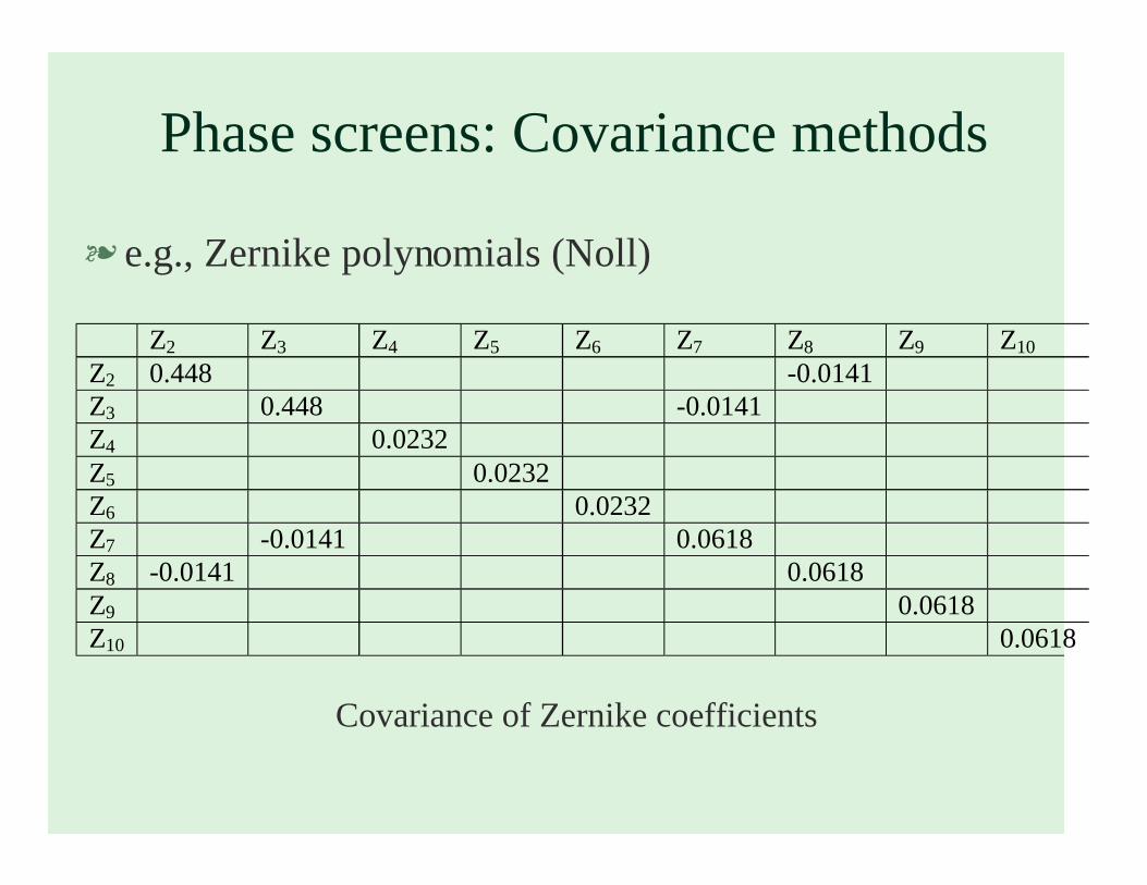
! e.g., Zernike polynomials (Noll)

Covariance of Zernike coefficients

Z2 Z3 Z4 Z5 Z6 Z7 Z8 Z9 Z10 Z2 0.448 -0.0141 Z3 0.448 -0.0141 Z4 0.0232 Z5 0.0232 Z6 0.0232 Z7 -0.0141 0.0618 Z8 -0.0141 0.0618 Z9 0.0618 Z10 0.0618

Phase screens: Covariance methods!Generate random Gaussian numbers with the right

covariance to obtain the coefficients.

!Multiply the basis function by the random coefficients.

!Generates phase screens with exact statistics.

! Computing large covariance matrices is difficult.

50 100 150 200 250 300

50

100

150

200

250

300

General points to note

!Kolmogorov turbulence is self-similar. Phase screens arescaled by multiplying the phase by .

! The phase is converted to a wavefront using .

! To compute discrete FTs, use the Fast Fourier Transform(FFT) which requires the number of points to be a powerof two (e.g., 256, 1024).

6/50 )/( rD

πφλ 2/=w

Propagation through the atmosphere

!Model turbulence as consisting of discrete layersat different heights between 0 and 20 km.

! In between the layers, there is no turbulence.

!There are several models for how many layersthere are and what their height, wind speed andturbulence strength is.

!The model is site dependent.

Propagation through the atmosphere

! The complex amplitude at height z+, u(z+), is 1.! The complex amplitude at height z-, u(z-), is exp[iφ1].! The light propagates from one layer to the next.! The phase of the turbulence at layer 2 is added:

u(0+)=u(0-)exp[iφ2].!How are the complex amplitudes at u(z-) and u(0+) related?

zφ1

φ2 0

Fresnel diffraction

! The complex amplitude at distance z is related to thecomplex amplitude at 0 by:

! If z is a few kilometers, this is very difficult to computebecause the chirp varies too quickly. Instead, we can thefact that the FT of a chirp is another chirp to give:

Chirp=exp[iαx2]

)]]2/(exp[),([)0,( 2 zikzuFu xxx ∝

]]]2/exp[)],([[)0,( 21 kizzuFFu xxx −∝ −

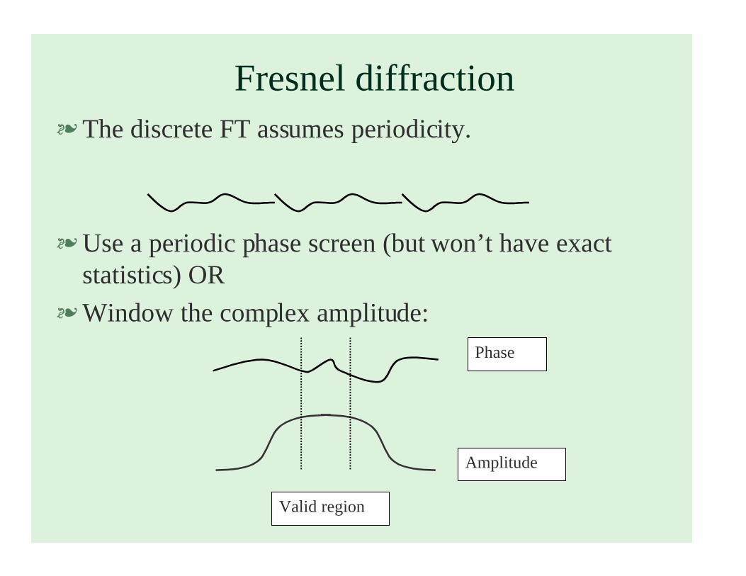
Fresnel diffraction! The discrete FT assumes periodicity.

!Use a periodic phase screen (but won’t have exactstatistics) OR

!Window the complex amplitude:Phase

Amplitude

Valid region

Temporal evolution! The atmosphere is “frozen” (Taylor hypothesis).

! Each layer of turbulence is blown by wind (a typicalvelocity is 10 m/s).

! If using a periodic phase screen, can wrap the screenaround again and again.

Summary of turbulence

!Have a small number of discrete turbulence layers atdifferent heights.

! Each layer is moving with its own velocity and direction.

! The propagation between each layer is performed usingFresnel diffraction.

! The complex amplitude at the focal plane is

where a(x) is the scintillation.

!Aberrations and corrective elements downstream add tothe phase but do not affect a(x).

)](exp[)()( xixaxu φ=

Telescope!The telescope defines the entrance pupil.

!Multiply the complex amplitude by the pupil.

Circular primary mirror withsecondary mirror obscuration

Keck Observatory entrance pupil

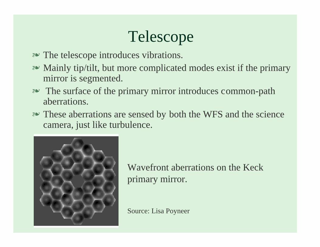
Telescope! The telescope introduces vibrations.! Mainly tip/tilt, but more complicated modes exist if the primary

mirror is segmented.! The surface of the primary mirror introduces common-path

aberrations.! These aberrations are sensed by both the WFS and the science

camera, just like turbulence.

Wavefront aberrations on the Keckprimary mirror.

Source: Lisa Poyneer

Imaging camera

!The Strehl ratio can be calculated via the Marechalapproximation: S=exp[-φ2]. Hence, the root-mean-squared (RMS) WF error defines the image quality.

!The complex amplitude at the focal plane is a scaledFT of the complex amplitude at the pupil. Hence theintensity is given by 2

2exp)()( dxx

fixuI

−= ∫ ξ

λπ

ξ

Imaging camera

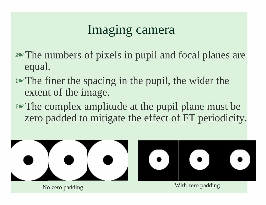
!The numbers of pixels in pupil and focal planes areequal.

!The finer the spacing in the pupil, the wider theextent of the image.

!The complex amplitude at the pupil plane must bezero padded to mitigate the effect of FT periodicity.

No zero padding With zero padding

WF Correction by parameterization!One can parameterize the wave-front.

" e.g., Zernikes, points at the corner (Fried) or in the middle ofsubapertures (Southwell).

" Less computationally intensive, but neglects fitting error.