marginal effects: discrete and continuous change

Marginal Effects for Continuous Variables

Marginal Effects for Continuous Variables Richard Williams, University of Notre Dame, https://www3.nd.edu/~rwilliam/

Last revised January 29, 2019 References: Long 1997, Long and Freese 2003 & 2006 & 2014, Cameron & Trivedi’s “Microeconomics Using Stata” Revised Edition, 2010

Overview. Marginal effects are computed differently for discrete (i.e. categorical) and continuous variables. This handout will explain the difference between the two. I personally find marginal effects for continuous variables much less useful and harder to interpret than marginal effects for discrete variables but others may feel differently. With binary independent variables, marginal effects measure discrete change, i.e. how do predicted probabilities change as the binary independent variable changes from 0 to 1? Marginal effects for continuous variables measure the instantaneous rate of change (defined shortly). They are popular in some disciplines (e.g. Economics) because they often provide a good approximation to the amount of change in Y that will be produced by a 1-unit change in Xk. But then again, they often do not. Example. We will show Marginal Effects at the Means (MEMS) for both the discrete and continuous independent variables in the following example. . use https://www3.nd.edu/~rwilliam/statafiles/glm-logit.dta, clear . logit grade gpa tuce i.psi, nolog Logistic regression Number of obs = 32 LR chi2(3) = 15.40 Prob > chi2 = 0.0015 Log likelihood = -12.889633 Pseudo R2 = 0.3740 ------------------------------------------------------------------------------ grade | Coef. Std. Err. z P>|z| [95% Conf. Interval] -------------+---------------------------------------------------------------- gpa | 2.826113 1.262941 2.24 0.025 .3507938 5.301432 tuce | .0951577 .1415542 0.67 0.501 -.1822835 .3725988 1.psi | 2.378688 1.064564 2.23 0.025 .29218 4.465195 _cons | -13.02135 4.931325 -2.64 0.008 -22.68657 -3.35613 ------------------------------------------------------------------------------

http://www3.nd.edu/%7Erwilliam/


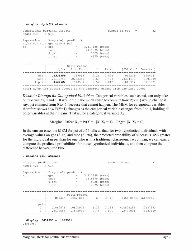
. margins, dydx(*) atmeans Conditional marginal effects Number of obs = 32 Model VCE : OIM Expression : Pr(grade), predict() dy/dx w.r.t. : gpa tuce 1.psi at : gpa = 3.117188 (mean) tuce = 21.9375 (mean) 0.psi = .5625 (mean) 1.psi = .4375 (mean) ------------------------------------------------------------------------------ | Delta-method | dy/dx Std. Err. z P>|z| [95% Conf. Interval] -------------+---------------------------------------------------------------- gpa | .5338589 .237038 2.25 0.024 .069273 .9984447 tuce | .0179755 .0262369 0.69 0.493 -.0334479 .0693989 1.psi | .4564984 .1810537 2.52 0.012 .1016397 .8113571 ------------------------------------------------------------------------------ Note: dy/dx for factor levels is the discrete change from the base level

Discrete Change for Categorical Variables. Categorical variables, such as psi, can only take on two values, 0 and 1. It wouldn’t make much sense to compute how P(Y=1) would change if, say, psi changed from 0 to .6, because that cannot happen. The MEM for categorical variables therefore shows how P(Y=1) changes as the categorical variable changes from 0 to 1, holding all other variables at their means. That is, for a categorical variable Xk

Marginal Effect Xk = Pr(Y = 1|X, Xk = 1) – Pr(y=1|X, Xk = 0) In the current case, the MEM for psi of .456 tells us that, for two hypothetical individuals with average values on gpa (3.12) and tuce (21.94), the predicted probability of success is .456 greater for the individual in psi than for one who is in a traditional classroom. To confirm, we can easily compute the predicted probabilities for those hypothetical individuals, and then compute the difference between the two. . margins psi, atmeans Adjusted predictions Number of obs = 32 Model VCE : OIM Expression : Pr(grade), predict() at : gpa = 3.117188 (mean) tuce = 21.9375 (mean) 0.psi = .5625 (mean) 1.psi = .4375 (mean) ------------------------------------------------------------------------------ | Delta-method | Margin Std. Err. z P>|z| [95% Conf. Interval] -------------+---------------------------------------------------------------- psi | 0 | .1067571 .0800945 1.33 0.183 -.0502252 .2637393 1 | .5632555 .1632966 3.45 0.001 .2432001 .8833109 ------------------------------------------------------------------------------ . display .5632555 - .1067571 .4564984


For categorical variables with more than two possible values, e.g. religion, the marginal effects show you the difference in the predicted probabilities for cases in one category relative to the reference category. So, for example, if relig was coded 1 = Catholic, 2 = Protestant, 3 = Jewish, 4 = other, the marginal effect for Protestant would show you how much more (or less) likely Protestants were to succeed than were Catholics, the marginal effect for Jewish would show you how much more (or less) likely Jews were to succeed than were Catholics, etc. Keep in mind that these are the marginal effects when all other variables equal their means (hence the term MEMs); the marginal effects will differ at other values of the Xs. Instantaneous rates of change for continuous variables. What does the MEM for gpa of .534 mean? It would be nice if we could say that a one unit increase in gpa will produce a .534 increase in the probability of success for an otherwise “average” individual. Sometimes statements like that will be (almost) true, but other times they will not. For example, if an “average” individual (average meaning gpa = 3.12, tuce = 21.94, psi = .4375) saw a one point increase in their gpa, here is how their predicted probability of success would change: . margins, at(gpa = (3.117188 4.117188)) atmeans Adjusted predictions Number of obs = 32 Model VCE : OIM Expression : Pr(grade), predict() 1._at : gpa = 3.117188 tuce = 21.9375 (mean) 0.psi = .5625 (mean) 1.psi = .4375 (mean) 2._at : gpa = 4.117188 tuce = 21.9375 (mean) 0.psi = .5625 (mean) 1.psi = .4375 (mean) ------------------------------------------------------------------------------ | Delta-method | Margin Std. Err. z P>|z| [95% Conf. Interval] -------------+---------------------------------------------------------------- _at | 1 | .2528205 .1052961 2.40 0.016 .046444 .459197 2 | .8510027 .1530519 5.56 0.000 .5510265 1.150979 ------------------------------------------------------------------------------ . display .8510027 - .2528205 .5981822

Note that (a) the predicted increase of .598 is actually more than the MEM for gpa of .534, and (b) in reality, gpa couldn’t go up 1 point for a person with an average gpa of 3.117. MEMs for continuous variables measure the instantaneous rate of change, which may or may not be close to the effect on P(Y=1) of a one unit increase in Xk. The appendices explain the concept in detail. What the MEM more or less tells you is that, if, say, Xk increased by some very small amount (e.g. .001), then P(Y=1) would increase by about .001*.534 = .000534, e.g.


. margins, at(gpa = (3.117188 3.118188)) atmeans noatlegend Adjusted predictions Number of obs = 32 Model VCE : OIM Expression : Pr(grade), predict() ------------------------------------------------------------------------------ | Delta-method | Margin Std. Err. z P>|z| [95% Conf. Interval] -------------+---------------------------------------------------------------- _at | 1 | .2528205 .1052961 2.40 0.016 .046444 .459197 2 | .2533547 .1053672 2.40 0.016 .0468388 .4598706 ------------------------------------------------------------------------------ . display .2533547 - .2528205 .0005342 Put another way, for a continuous variable Xk,

Marginal Effect of Xk = limit [Pr(Y = 1|X, Xk+Δ) – Pr(y=1|X, Xk)] / Δ ] as Δ gets closer and closer to 0

The appendices show how to get an exact solution for this. There is no guarantee that a bigger increase in Xk, e.g. 1, would produce an increase of 1*.534=.534. This is because the relationship between Xk and P(Y = 1) is nonlinear. When Xk is measured in small units, e.g. income in dollars, the effect of a 1 unit increase in Xk may match up well with the MEM for Xk. But, when Xk is measured in larger units (e.g. income in millions of dollars) the MEM may or may not provide a very good approximation of the effect of a one unit increase in Xk. That is probably one reason why instantaneous rates of change for continuous variables receive relatively little attention, at least in Sociology. More common are approaches which focus on discrete changes. Conclusion. Marginal effects can be an informative means for summarizing how change in a response is related to change in a covariate. For categorical variables, the effects of discrete changes are computed, i.e., the marginal effects for categorical variables show how P(Y = 1) is predicted to change as Xk changes from 0 to 1 holding all other Xs equal. This can be quite useful, informative, and easy to understand. For continuous independent variables, the marginal effect measures the instantaneous rate of change. If the instantaneous rate of change is similar to the change in P(Y=1) as Xk increases by one, this too can be quite useful and intuitive. However, there is no guarantee that this will be the case; it will depend, in part, on how Xk is scaled. Subsequent handouts will show how the analysis of discrete changes in continuous variables can make their effects more intelligible.


Appendix A: AMEs for continuous variables, computed manually (Optional)

Calculus can be used to compute marginal effects, but Cameron and Trivedi (Microeconometrics using Stata, Revised Edition, 2010, section 10,6.10, pp. 352 – 354) show that they can also be computed manually. The procedure is as follows: Compute the predicted values using the observed values of the variables. We will call this prediction1. Change one of the continuous independent variables by a very small amount. Cameron and Trivedi suggest using the standard deviation of the variable divided by 1000. We will refer to this as delta (Δ). Compute the new predicted values for each case. Call this prediction2. For each case, compute

𝑥𝑥𝑥𝑥𝑥𝑥 = 𝑝𝑝𝑝𝑝𝑥𝑥𝑝𝑝𝑝𝑝𝑝𝑝𝑝𝑝𝑝𝑝𝑝𝑝𝑝𝑝2 − 𝑝𝑝𝑝𝑝𝑥𝑥𝑝𝑝𝑝𝑝𝑝𝑝𝑝𝑝𝑝𝑝𝑝𝑝𝑝𝑝1

𝛥𝛥

Compute the mean value of xme. This is the AME for the variable in question. Here is an example: . * Appendix A: Compute AMEs manually . webuse nhanes2f, clear . * For convenience, keep only nonmissing cases . keep if !missing(diabetes, female, age) (2 observations deleted) . clonevar xage = age . sum xage Variable | Obs Mean Std. Dev. Min Max -------------+-------------------------------------------------------- xage | 10335 47.56584 17.21752 20 74 . gen xdelta = r(sd)/1000 . logit diabetes i.female xage, nolog Logistic regression Number of obs = 10335 LR chi2(2) = 345.87 Prob > chi2 = 0.0000 Log likelihood = -1826.1338 Pseudo R2 = 0.0865 ------------------------------------------------------------------------------ diabetes | Coef. Std. Err. z P>|z| [95% Conf. Interval] -------------+---------------------------------------------------------------- 1.female | .1549701 .0940619 1.65 0.099 -.0293878 .3393279 xage | .0588637 .0037282 15.79 0.000 .0515567 .0661708 _cons | -6.276732 .2349508 -26.72 0.000 -6.737227 -5.816237 ------------------------------------------------------------------------------


. margins, dydx(xage) Average marginal effects Number of obs = 10335 Model VCE : OIM Expression : Pr(diabetes), predict() dy/dx w.r.t. : xage ------------------------------------------------------------------------------ | Delta-method | dy/dx Std. Err. z P>|z| [95% Conf. Interval] -------------+---------------------------------------------------------------- xage | .0026152 .000188 13.91 0.000 .0022468 .0029836 ------------------------------------------------------------------------------ . predict xage1 (option pr assumed; Pr(diabetes)) . replace xage = xage + xdelta xage was byte now float (10335 real changes made) . predict xage2 (option pr assumed; Pr(diabetes)) . gen xme = (xage2 - xage1) / xdelta . sum xme Variable | Obs Mean Std. Dev. Min Max -------------+-------------------------------------------------------- xme | 10335 .0026163 .0020192 .0003549 .0073454 . end of do-file


Appendix B: Technical Discussion of Marginal Effects (Optional) In binary regression models, the marginal effect is the slope of the probability curve relating Xk to Pr(Y=1|X), holding all other variables constant. But what is the slope of a curve??? A little calculus review will help make this clearer. Simple Explanation. Draw a graph of F(Xk) against Xk, holding all the other X’s constant (e.g. at their means). Chose 2 points, [Xk, F(Xk)] and [Xk+ Δ, F(Xk+ Δ)]. When Δ is very very small, the slope of the line connecting the two points will equal or almost equal the marginal effect of Xk. More Detailed Explanation. Again, what is the slope of a curve? Intuitively, think of it this way. Draw a graph of F(X) against X, e.g. F(X) = X2. Chose specific values of X and F(X), e.g. [2, F(2)]. Choose another point, e.g. [8, F(8)]. Draw a line connecting the points. This line has a slope. The slope is the average rate of change. Now, choose another point that is closer to [2, F(2)], e.g. [7, F(7)]. Draw a line connecting these points. This too will have a slope. Keep on choosing points that are closer to [2, F(2)]. The instantaneous rate of change is the limit of the slopes for the lines connecting [X, F(X)] and [X+Δ, F(X + Δ)] as Δ gets closer and closer to 0.

Source: http://www.ugrad.math.ubc.ca/coursedoc/math100/notes/derivative/slope.html

Last accessed January 29, 2019 See the above link for more information

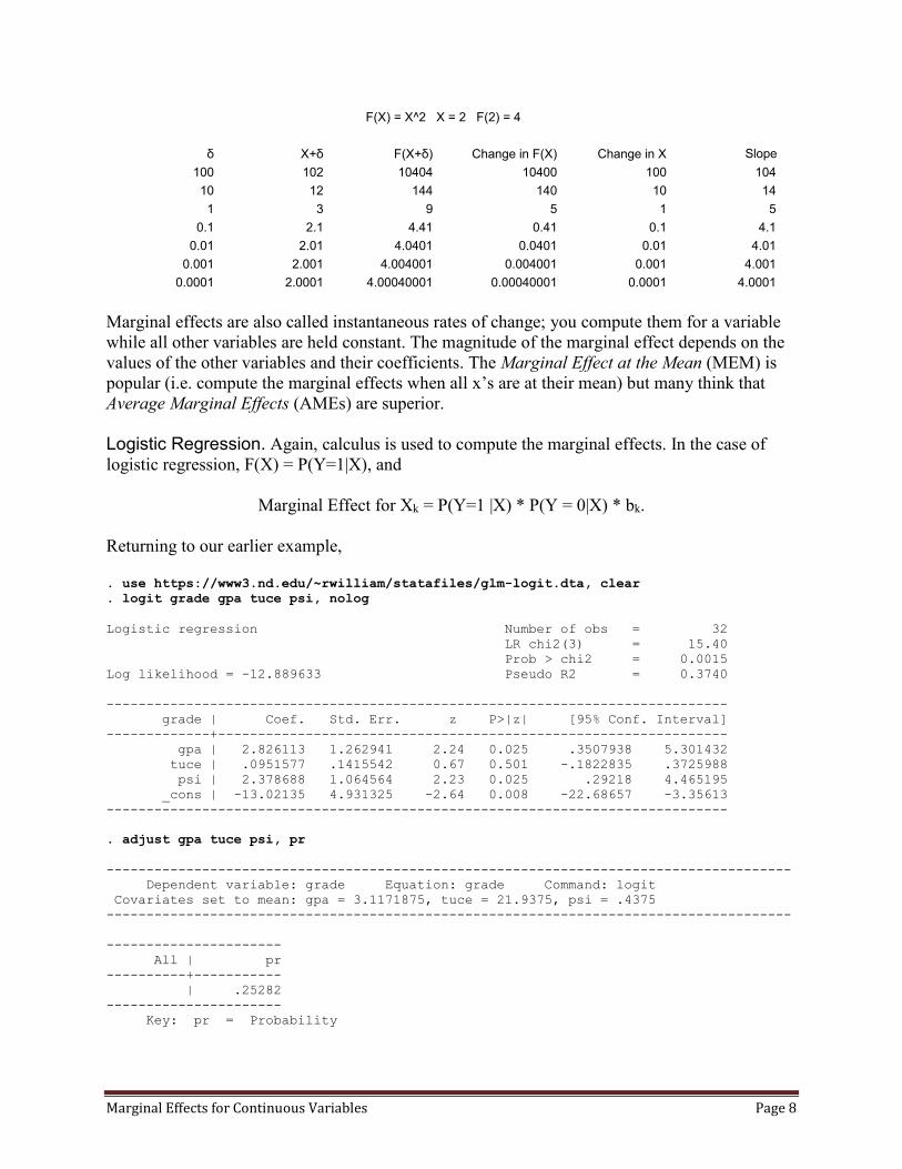
Calculus is used to compute slopes (& marginal effects). For example, if Y = X2, then the slope is 2X. Hence, if X = 2, the slope is 4. The following table illustrates this. Note that, as Δ gets smaller and smaller, the slope gets closer and closer to 4.

http://www.ugrad.math.ubc.ca/coursedoc/math100/notes/derivative/slope.html


F(X) = X^2 X = 2 F(2) = 4

δ X+δ F(X+δ) Change in F(X) Change in X Slope100 102 10404 10400 100 10410 12 144 140 10 141 3 9 5 1 5

0.1 2.1 4.41 0.41 0.1 4.10.01 2.01 4.0401 0.0401 0.01 4.01

0.001 2.001 4.004001 0.004001 0.001 4.0010.0001 2.0001 4.00040001 0.00040001 0.0001 4.0001

Marginal effects are also called instantaneous rates of change; you compute them for a variable while all other variables are held constant. The magnitude of the marginal effect depends on the values of the other variables and their coefficients. The Marginal Effect at the Mean (MEM) is popular (i.e. compute the marginal effects when all x’s are at their mean) but many think that Average Marginal Effects (AMEs) are superior. Logistic Regression. Again, calculus is used to compute the marginal effects. In the case of logistic regression, F(X) = P(Y=1|X), and

Marginal Effect for Xk = P(Y=1 |X) * P(Y = 0|X) * bk. Returning to our earlier example, . use https://www3.nd.edu/~rwilliam/statafiles/glm-logit.dta, clear . logit grade gpa tuce psi, nolog Logistic regression Number of obs = 32 LR chi2(3) = 15.40 Prob > chi2 = 0.0015 Log likelihood = -12.889633 Pseudo R2 = 0.3740 ------------------------------------------------------------------------------ grade | Coef. Std. Err. z P>|z| [95% Conf. Interval] -------------+---------------------------------------------------------------- gpa | 2.826113 1.262941 2.24 0.025 .3507938 5.301432 tuce | .0951577 .1415542 0.67 0.501 -.1822835 .3725988 psi | 2.378688 1.064564 2.23 0.025 .29218 4.465195 _cons | -13.02135 4.931325 -2.64 0.008 -22.68657 -3.35613 ------------------------------------------------------------------------------ . adjust gpa tuce psi, pr -------------------------------------------------------------------------------------- Dependent variable: grade Equation: grade Command: logit Covariates set to mean: gpa = 3.1171875, tuce = 21.9375, psi = .4375 -------------------------------------------------------------------------------------- ---------------------- All | pr ----------+----------- | .25282 ---------------------- Key: pr = Probability


. mfx Marginal effects after logit y = Pr(grade) (predict) = .25282025 ------------------------------------------------------------------------------ variable | dy/dx Std. Err. z P>|z| [ 95% C.I. ] X ---------+-------------------------------------------------------------------- gpa | .5338589 .23704 2.25 0.024 .069273 .998445 3.11719 tuce | .0179755 .02624 0.69 0.493 -.033448 .069399 21.9375 psi*| .4564984 .18105 2.52 0.012 .10164 .811357 .4375 ------------------------------------------------------------------------------ (*) dy/dx is for discrete change of dummy variable from 0 to 1

Looking specifically at GPA – when all variables are at their means, pr(Y=1|X) = .2528, Pr(Y=0|X) = .7472, and bGPA = 2.826113. The marginal effect at the mean for GPA is therefore

Marginal Effect of GPA = P(Y=1 |X) * P(Y = 0|X) * bGPA = .2528 * .7472 * 2.826113 = .5339 The following table again shows you that, in logistic regression, as the distance between two points gets smaller and smaller, i.e. as Δ gets closer and closer to 0, the slope of the line connecting the points gets closer and closer to the marginal effect.

Logistic Regression

F(X,GPA) = P(Y=1|X, GPA) GPA=3.11719 Other X's at Mean F(X,3.11719) = .25282025107643

δ GPA+δ F(X,GPA+δ) Change in F(X,GPA) Change in GPA Slope10 13.11719 1 0.747179749 10 0.07471797491 4.11719 0.851002558 0.598182307 1 0.5981823074

0.1 3.21719 0.309808293 0.056988042 0.1 0.56988041650.05 3.16719 0.280431679 0.027611428 0.05 0.55222856400.01 3.12719 0.258196038 0.005375787 0.01 0.5375787403

0.001 3.11819 0.253354486 0.000534235 0.001 0.53423507880.0001 3.11729 0.252873644 5.3393E-05 0.0001 0.5339297264

Probit. In probit, the marginal effect is

Marginal Effect for Xk = Φ(XB) * bk where Φ is the probability density function for a standardized normal variable. For example, as this diagram shows, Φ(0) = .399:


Example: . use https://www3.nd.edu/~rwilliam/statafiles/glm-logit.dta, clear . probit grade gpa tuce psi, nolog Probit estimates Number of obs = 32 LR chi2(3) = 15.55 Prob > chi2 = 0.0014 Log likelihood = -12.818803 Pseudo R2 = 0.3775 ------------------------------------------------------------------------------ grade | Coef. Std. Err. z P>|z| [95% Conf. Interval] -------------+---------------------------------------------------------------- gpa | 1.62581 .6938818 2.34 0.019 .2658269 2.985794 tuce | .0517289 .0838901 0.62 0.537 -.1126927 .2161506 psi | 1.426332 .595037 2.40 0.017 .2600814 2.592583 _cons | -7.45232 2.542467 -2.93 0.003 -12.43546 -2.469177 ------------------------------------------------------------------------------ . mfx Marginal effects after probit y = Pr(grade) (predict) = .26580809 ------------------------------------------------------------------------------ variable | dy/dx Std. Err. z P>|z| [ 95% C.I. ] X ---------+-------------------------------------------------------------------- gpa | .5333471 .23246 2.29 0.022 .077726 .988968 3.11719 tuce | .0169697 .02712 0.63 0.531 -.036184 .070123 21.9375 psi*| .464426 .17028 2.73 0.006 .130682 .79817 .4375 ------------------------------------------------------------------------------ (*) dy/dx is for discrete change of dummy variable from 0 to 1 . * marginal change for GPA. The invnorm function gives us the Z-score for the stated . * prob of success. The normalden function gives us the pdf value for that Z-score. . display invnorm(.2658) -.62556546 . display normalden(invnorm(.2658)) .32804496 . display normalden(invnorm(.2658)) * 1.62581 .53333878

Marginal Effect for GPA = Φ(XB) * bk = .32804496 * 1.62581 = .5333 The following table again shows you that, in a probit model, as the distance between two points gets smaller and smaller, i.e. as Δ gets closer and closer to 0, the slope of the line connecting the points gets closer and closer to the marginal effect.


Probit

F(X,GPA) = P(Y=1|X, GPA) GPA=3.11719 Other X's at Mean F(X,3.11719) = .26580811

δ GPA+δ F(X,GPA+δ) Change in F(X,GPA) Change in GPA Slope10 13.11719 1 0.73419189 10 0.07341918901 4.11719 0.841409951 0.575601841 1 0.5756018408

0.1 3.21719 0.321696605 0.055888495 0.1 0.55888495450.01 3.12719 0.27116854 0.00536043 0.01 0.5360430345

0.001 3.11819 0.266341711 0.000533601 0.001 0.53360104790.0001 3.11729 0.26586143 5.33203E-05 0.0001 0.5332029760

Using the margins command for MEMs & AMEs, . quietly probit grade gpa tuce i.psi, nolog . margins, dydx(*) atmeans Conditional marginal effects Number of obs = 32 Model VCE : OIM Expression : Pr(grade), predict() dy/dx w.r.t. : gpa tuce 1.psi at : gpa = 3.117188 (mean) tuce = 21.9375 (mean) 0.psi = .5625 (mean) 1.psi = .4375 (mean) ------------------------------------------------------------------------------ | Delta-method | dy/dx Std. Err. z P>|z| [95% Conf. Interval] -------------+---------------------------------------------------------------- gpa | .5333471 .2324641 2.29 0.022 .0777259 .9889683 tuce | .0169697 .0271198 0.63 0.531 -.0361841 .0701235 1.psi | .464426 .1702807 2.73 0.006 .1306819 .7981701 ------------------------------------------------------------------------------ Note: dy/dx for factor levels is the discrete change from the base level. . margins, dydx(*) Average marginal effects Number of obs = 32 Model VCE : OIM Expression : Pr(grade), predict() dy/dx w.r.t. : gpa tuce 1.psi ------------------------------------------------------------------------------ | Delta-method | dy/dx Std. Err. z P>|z| [95% Conf. Interval] -------------+---------------------------------------------------------------- gpa | .3607863 .1133816 3.18 0.001 .1385625 .5830102 tuce | .0114793 .0184095 0.62 0.533 -.0246027 .0475612 1.psi | .3737518 .1399913 2.67 0.008 .099374 .6481297 ------------------------------------------------------------------------------ Note: dy/dx for factor levels is the discrete change from the base level.

As a sidelight, note that the marginal effects (both MEMs and AMEs) for probit are very similar to the marginal effects for logit. This is usually the case.


OLS. Here is what you get when you compute the marginal effects for OLS: . use https://www3.nd.edu/~rwilliam/statafiles/glm-reg.dta, clear . reg income educ jobexp black Source | SS df MS Number of obs = 500 -------------+------------------------------ F( 3, 496) = 787.14 Model | 33206.4588 3 11068.8196 Prob > F = 0.0000 Residual | 6974.79047 496 14.0620776 R-squared = 0.8264 -------------+------------------------------ Adj R-squared = 0.8254 Total | 40181.2493 499 80.5235456 Root MSE = 3.7499 ------------------------------------------------------------------------------ income | Coef. Std. Err. t P>|t| [95% Conf. Interval] -------------+---------------------------------------------------------------- educ | 1.840407 .0467507 39.37 0.000 1.748553 1.932261 jobexp | .6514259 .0350604 18.58 0.000 .5825406 .7203111 black | -2.55136 .4736266 -5.39 0.000 -3.481921 -1.620798 _cons | -4.72676 .9236842 -5.12 0.000 -6.541576 -2.911943 ------------------------------------------------------------------------------ . margins, dydx(*) atmeans Conditional marginal effects Number of obs = 500 Model VCE : OLS Expression : Linear prediction, predict() dy/dx w.r.t. : educ jobexp black at : educ = 13.16 (mean) jobexp = 13.52 (mean) black = .2 (mean) ------------------------------------------------------------------------------ | Delta-method | dy/dx Std. Err. z P>|z| [95% Conf. Interval] -------------+---------------------------------------------------------------- educ | 1.840407 .0467507 39.37 0.000 1.748777 1.932036 jobexp | .6514259 .0350604 18.58 0.000 .5827087 .7201431 black | -2.55136 .4736266 -5.39 0.000 -3.479651 -1.623069 ------------------------------------------------------------------------------ . margins, dydx(*) Average marginal effects Number of obs = 500 Model VCE : OLS Expression : Linear prediction, predict() dy/dx w.r.t. : educ jobexp black ------------------------------------------------------------------------------ | Delta-method | dy/dx Std. Err. z P>|z| [95% Conf. Interval] -------------+---------------------------------------------------------------- educ | 1.840407 .0467507 39.37 0.000 1.748777 1.932036 jobexp | .6514259 .0350604 18.58 0.000 .5827087 .7201431 black | -2.55136 .4736266 -5.39 0.000 -3.479651 -1.623069 ------------------------------------------------------------------------------ The marginal effects are the same as the slope coefficients. This is because relationships are linear in OLS regression and do not vary depending on the values of the other variables.

marginal effects: discrete and continuous change

Documents