Universidade de Aveiro

2019

Departamento de Ambiente e Ordenamento

Maria Salomé Costa Silva

Impactes, custos e benefícios de soluções baseadas na natureza para a adaptação urbana às mudanças climáticas

Multiple impacts, costs and (co-) benefits from nature-based solutions for urban climate change adaptation

Universidade de Aveiro

2019

Departamento de Ambiente e Ordenamento

Maria Salomé Costa Silva

Impactes, custos e benefícios de soluções baseadas na natureza para a adaptação urbana às mudanças climáticas

Multiple impacts, costs and (co-) benefits from nature-based solutions for urban climate change adaptation

Dissertação apresentada à Universidade de Aveiro para cumprimento dos requisitos necessários à obtenção do grau de Mestre em Engenharia do Ambiente, realizada sob a orientação científica do Professor Doutor Peter Roebeling, Equiparado a Investigador Auxiliar no Departamento de Ambiente e Ordenamento da Universidade de Aveiro e co-orientação do Doutor Ricardo Martins, Investigador Doutorado no Departamento de Ambiente e Ordenamento da Universidade de Aveiro.

This thesis was developed in the context of the UNaLab project (https://www.unalab.eu/), undertaken by a consortium led by VTT and in which the UA is consortium partner as well as work package leader (Monitoring and impact assessment). The UNaLab project has received funding from the European Union Horizon 2020 research and innovation programme under Grant Agreement No. 730052, Topic: SCC-2-2016-2017: Smart Cities and Communities Nature based solutions.

o júri

presidente Professor Doutor Mário Miguel Azevedo Cerqueira

Professor Auxiliar, Universidade de Aveiro

Doutor Peter Cornelis Roebeling Equiparado a Investigador Auxiliar, Universidade de Aveiro (Orientador)

Professor Doutor José Manuel Gaspar Martins Professor Auxiliar, Universidade de Aveiro (Arguente)

palavras- chave Soluções baseadas na natureza; alterações climáticas; urbanização; dano de cheias; valorização do mercado imobiliário

Resumo

O desenvolvimento urbano contínuo e rápido trouxe mudanças nos padrões de uso do solo, tendo ocorrido uma grande conversão da paisagem natural em urbana e uma impermeabilização dessas superfícies. Isso trouxe problemas de diferentes níveis que se tornaram exacerbados com as mudanças climáticas: aumento do risco de inundações, "ilhas urbanas de calor", aumento da concentração de poluentes atmosféricos e declínio da qualidade de vida. As soluções atuais para a adaptação aos desafios urbanos geralmente exigem mudanças na paisagem, manutenção e desvalorizam ao longo do tempo. As soluções baseadas na natureza (SBN) vieram como soluções eficientes e amigas do ambiente que, além de agregar valor à estética da paisagem urbana, podem ajudar a mitigar e adaptar as cidades aos desafios das mudanças climáticas e da urbanização. O objetivo desta tese é avaliar os múltiplos impactos, custos e benefícios da implementação das SBN, com um foco específico nos danos causados pelas inundações, expansão e gentrificação urbana e valorização do mercado imobiliário. Para este fim, dois modelos da Systemic Decision Support Tool (SDST) são usados para avaliar os impactos da SBN sobre o risco de inundação (usando o InfoWorks) e sobre o mercado imobiliário (usando o SULD). Um caso de estudo é fornecido para a cidade de Eindhoven, na Holanda. Os resultados mostram que a implementação de soluções baseadas na natureza conduz a um aumento do valor imobiliário (+6,1 M€/ano) devido à melhoria da estética do meio urbano e tem também um impacto nos danos causados pelas inundações, atuando na mitigação das inundações e reduzindo os custos dos danos (-27,4k€/ano).Para além das suas principais funções, as SBN mostram também um efeito nos padrões de distribuição da população, favorecendo a densificação urbana em detrimento dos processos de expansão urbana.

keywords nature-based solutions; climate change; urbanization; flood damage; real estate valuation

Abstract

The on-going and fast-urban development brought along changes in land-use patterns having resulted in a major conversion of natural landscapes into urban ones and a subsequent impermeabilization of surfaces. This came with problems of different dimensions which are expected to be exacerbated by climate change: increased flood risk, “urban heat islands”, increased air pollution and reduced quality of life. Current ‘hard’ engineering solutions to adapt to urban challenges usually require landscape changes, maintenance and depreciate over time. Nature-based solutions came as efficient and eco-friendlier solutions that besides adding value to urban landscape aesthetics can help mitigate and adapt cities to climate-change and urbanization challenges. The objective of this thesis is to evaluate the multiple impacts, costs and benefits of NBS implementation, with a specific focus on flood damage and sprawl, gentrification and real estate valuation. To this end, two models of the Systemic Decision Support Tool (SDST) are used to assess the impacts of NBS on flood risk (using InfoWORKS) and sprawl, gentrification and real estate valuation (using SULD). A case study is provided for the city of Eindhoven in the Netherlands. Results show that the implementation of nature-based solutions leads to an increase in real estate values (+6.1 M€/yr) due to upgraded aesthetics and has an impact on flood damages acting on flood mitigation and reducing damage costs (-27.4 k€/yr). Besides its main functions, NBS also show an effect on population distribution patterns – favouring urban densification over urban sprawl processes.

xi

Table of contents

Table of contents .................................................................................................................. xi

List of figures ..................................................................................................................... xiii

List of tables ........................................................................................................................ xv

Abbreviations .................................................................................................................... xvii

1.Introduction ........................................................................................................................ 1

1.1 Problem setting ................................................................................................................ 1

1.2 State of knowledge ..................................................................................................... 4

1.3 Objective .......................................................................................................................... 4

1.4 Outline ............................................................................................................................. 6

2. Literature review................................................................................................................ 7

2.1 Urban heating .................................................................................................................. 7

2.1.1 Context ......................................................................................................................... 7

2.1.2 Impact Assessment ..................................................................................................... 10

2.2 Air pollution .................................................................................................................. 14

2.2.1 Context ....................................................................................................................... 14

2.2.2 Impact assessment ...................................................................................................... 17

2.3 Urban flooding ............................................................................................................... 22

2.3.1 Context ....................................................................................................................... 22

2.3.2 Impact Assessment ..................................................................................................... 24

2.4 Sprawl, gentrification and real estate valuation............................................................. 25

3.Methodology ..................................................................................................................... 28

3.1 Environmental assessment ............................................................................................. 29

3.1.1 InfoWORKS ............................................................................................................... 29

xii

3.1.2 SULD .......................................................................................................................... 31

3.2 Compilation and synthesis of the relationship between physical and economic impacts

............................................................................................................................................. 35

4. Case study description ..................................................................................................... 38

4.1 Eindhoven ...................................................................................................................... 38

4.2 Scenario description ...................................................................................................... 40

4.2.1 NBS scenario .............................................................................................................. 40

5. Results and discussion ..................................................................................................... 42

5.1 Flooding ......................................................................................................................... 42

5.2 Sprawl, gentrification and real estate valuation............................................................. 46

5.3 Total economic impacts of NBS .................................................................................... 49

6. Conclusions ..................................................................................................................... 51

7. Future recommendations ................................................................................................. 53

Annex .................................................................................................................................. 62

xiii

List of figures

Figure 1- Urban and rural population in the world over the period 1950-2050, as projected

by the UN World Urbanization Prospects (United Nations, 2014) ....................................... 1

Figure 2- Schematic representation of the SDST in which will be included the quantification

of the associated individual costs/benefits applied to four of the urban challenges addressed

by the SDST (urban heat, air quality, flooding and water quality)individually and the total

gains ....................................................................................................................................... 5

Figure 3- Relationship between temperature increasing and productivity loss (Vivid

Economics, 2017) ................................................................................................................ 12

Figure 4– Relationship between temperature and energy demand in Qatar (Gastli et al., 2013)

............................................................................................................................................. 13

Figure 5- Number of premature deaths per year and per million people caused by outdoor

air pollution (particulate matter and ozone) in 2010 and its estimation for 2060 for different

countries (OECD, 2016) ...................................................................................................... 17

Figure 6- Depth Damage function for the different sectors in Germany’s economy (Prahl

et al., 2018) .......................................................................................................................... 24

Figure 7 - Schematic Representation of the Impact Pathway Approach (adapted) ............. 28

Figure 8 – “Preissmann Slot”- conceptual vertical and narrow slot providing a conceptual

free surface condition for the flow when the water level is above the top of a closed conduit

............................................................................................................................................. 31

Figure 9 – Percentage of damage for residential buildings according to flood depth ......... 36

Figure 10 - Percentage of damage for commercial and industrial buildings according to flood

depth .................................................................................................................................... 37

Figure 11 - Percentage of damage for infrastructure according to flood depth ................... 37

Figure 12 - Population trend in Eindhoven ......................................................................... 39

Figure 13 - Land Use for the inner-ring of Eindhoven ........................................................ 39

Figure 14 - Multiple NBS implementation scenarios in the city centre of Eindhoven,

Netherlands .......................................................................................................................... 40

Figure 15 – Current situation (2015) – flood depth in Eindhoven (city centre) for a rain event

of return period of 20 years where the main flood areas are highlighted ............................ 43

xiv

Figure 16 - Creation of a conditional statement in QGIS field calculator for flood damage

calculation ............................................................................................................................ 43

Figure 17 - Baseline (blue) and NBS (green) flood streams in a part of the city ................ 44

Figure 18 – NBS spatial distribution with the main flood mitigation areas identified ........ 45

Figure 19 - Difference between NBS and baseline scenario for household density (scenario

1-5) ...................................................................................................................................... 47

Figure 20 - Difference between NBS and baseline scenario for distance to higher value

green/blue spaces (m) .......................................................................................................... 48

Figure 21 - Difference between NBS and baseline scenario for house price (€/m2) ........... 48

xv

List of tables

Table 1 - Compilation of studies that prove the impact of NBS implementation on

temperature and its respective co-benefits............................................................................. 9

Table 2 - Excess mortality attributed to hot summer/heat waves period in Europe adapted

from (Haines et al. (2006).................................................................................................... 11

Table 3 - Compilation of studies that prove the impact of NBS implementation on air quality

and its respective co-benefits ............................................................................................... 16

Table 4 – Health effects related with PM10 exposure, concentration-response functions

(CRF) and of respective economic valuation (base costs €2015) ....................................... 20

Table 5 - Health effects related with PM2.5 exposure, concentration-response functions

(CRF) and of respective economic valuation (base costs €2015) ....................................... 21

Table 6 - Health effects related with NO2 exposure, concentration-response functions (CRF)

and of respective economic valuation (base costs €2015) ................................................... 21

Table 7 - Examples of studies that quantify the impact of NBS implementation on flood risk

and its respective co-benefits ............................................................................................... 23

Table 8 - Compilation of studies that prove the impact of NBS implementation on urban

densification and its respective co-benefits ......................................................................... 27

Table 9 - Description of the NBS implementation scenarios .............................................. 41

Table 10- Flood damage costs for a return period of 20 years: Baseline and NBS

implementation scenario for Eindhoven (2015) .................................................................. 44

Table 11- Real estate: annual rental value (M€/yr) for baseline and NBS implementation

scenario for Eindhoven ........................................................................................................ 49

Table 12 - Total Avoided costs and benefits from NBS implementation .......................... 50

xvi

xvii

Abbreviations

AR – Attributable Risk

CPI – Consumer Price Index

CRF- Concentration-Response Function

CVD – Cardiovascular Diseases

COPD – Chronic Obstructive Pulmonary Diseases

ES – Ecosystem Services

EU – European Union

GI – Green Infrastructure

GIS – Geographic Information System

HA – Hospital Admissions

IPCC – Intergovernmental Panel on Climate Change

IR – Inflation Rate

Inhab – Inhabitants

NBS – Nature Based Solutions

NO2 – Nitrogen Dioxide

PM2.5 – Particulate Matter (diameter of 2.5 μm or less)

PM10 – Particulate Matter (diameter of 10 μm or less)

RR – Relative Risk

SDST – Systemic Decision Support Tool

VOLY – Value Of a Life Year

YOLL – Year Of Life Lost

VSL – Value of a Statistical Life

xviii

1

1.Introduction

1.1 Problem setting

The promise of better jobs and business opportunities as well as economic and social

benefits, such as higher levels of education, effective healthcare and greater access to social

and cultural services, has driven populations to move from rural to urban areas in search of

a better lifestyle and quality of life. The migration of the population from rural to urban areas

leads to an expansion and growth in size of the cities, requiring more land and space to

accommodate this population. Currently the percentage of people living in urban areas (54%)

exceeds the population living in rural areas, and the future tendency is not only the growth

of the overall population but also the increase of the urbanization – with two-thirds of the

world´s population living in urban areas by 2050 (see Figure 1) (United Nations, 2014),

resulting in an sprawl/densification of urban areas (Haaland & van den Bosch, 2015).

Figure 1- Urban and rural population in the world over the period 1950-2050, as projected by the UN

World Urbanization Prospects (United Nations, 2014)

The economic growth of cities leads to a continuous growing of the population, migration to

urban areas and expansion of the industry putting at stake the cities’ capacity to deal with

the increasing demands and incoming pressures on water resources supply and management.

This phenomenon induces a conversion of green and agricultural areas, as well as natural

wetlands, into urban ecosystems, resulting in a waterproofing of the urban surface in which

2

pollutants from anthropogenic activities (nonpoint source pollution) are accumulated and

runoff into the streams, thus affecting and degrading water quality (Ren et al., 2003; Jung et

al., 2016). The increase of these impervious surfaces leads to a decline on the soil natural

capacity to infiltrate and store water, thus resulting in surface runoff and higher flooding risk

frequencies (Chan et al., 2018).

Urban areas also affect and change local climate as compared to rural areas, as they present

a quite different climate dynamic. The urban medium is composed by a high percentage of

radiation-absorbing materials and in combination with the increase in anthropogenic heat

sources, due to human activities and energy consumption and the lack of green infrastructure,

this results in a significant increase in temperature relative to the surrounding rural areas

(Seto et al., 2011).

Nowadays numerous cities struggle to keep their air quality standards to levels in a way of

not causing harmful impacts on the health and environment. The major contributor for the

poor air quality within the cities is anthropogenic emissions derived from urban population

and economic growth of cities, causing the consequent increase in the emission and

concentration of air pollutants, among them: ozone (O3), carbon monoxide (CO), sulphur

dioxide (SO2) and particulate matter with an aerodynamic diameter less than 2,5 µm

(PM2.5) and 10 µm (PM10) (Nowak et al., 2018 ; Zhou et al., 2018).

The lack of proper and sufficient green/blue infrastructure through the urban space, makes

these types of amenities valuable for its residents, influencing buyers’ choices when

choosing a property, consequently impacting the local real estate market (Mayor et al.,

2009).

Although there are advantages of urban areas over rural areas in several aspects (economy,

healthcare, education, etc), urban living conditions and quality of life are deteriorating over

time due to the lack of adequate infrastructure, policies and a strong and solid urban planning

(United Nations, 2014).

Current cities are vulnerable and unprepared to deal with climate change, so there is an

emergent need for urban areas to adapt and become more resilient to climate change and on-

going urbanization impacts (Haase, 2015). At the same time, there are opportunities to

address the challenges that threat cities’ sustainability by ensuring a better resource

3

efficiency and protecting them against unwelcome foreseeable future changes (European

Commission, 2015).

So far, the adaptation and mitigation to climate change has been relying on grey

infrastructure or technological solutions. Grey infrastructures are engineered, and physical

structures/systems made by long-lasting materials, which usually can be monitored,

replicable and controlled over time and usually require limited amount of land. These

infrastructures usually are conceived for a limited set of specific functions and may include

“dikes, floodgates, sea walls and breakwaters for riverine and coastal flood protection,

drainage systems for storm water management such as storm sewers, pipes, detention basins”

(Depietri & Mcphearson, 2017). These types of solutions usually require maintenance,

have significant changes in the landscape, are difficult to adapt to changing conditions,

have high implementation costs moreover, they can depreciate in performance over time

and may have also some environmental impacts (WRI, n.d).

Nature-based solutions (NBS) are solutions developed to cope with sustainabilty challenges

which are inspired and based in natural processes that are locally adaptable, resource-

efficient and help build up resilience in cities (Fini et al., 2017). NBS sustain itselves and

rely on ecossystems’ functioning as the fundamental part and pillar for climate change

adaptation and mitigation (European Commission, 2015). Hence, the implementation of

NBS, green and blue infrascture in urban areas - green roofs, floodplain restoration, green

urban spaces, street trees, constructed wetlands, pervious pavement, etc., (Depietri &

Mcphearson, 2017; Lafortezza et al., 2018; Sörensen, 2018) has been increasing in order to

adress the challenges and pressures that threatens society, being this solutions recognised

for their capacity of not only “protecting, sustainably managing and restore natural or

modified ecosystems” (Walters et al., 2016) but also to perform different functions and

generate additional environmental, economic and social benefits simultaneously and over

time (Kabisch et al., 2016). When comparing gray to green infrastructure most studies show

the last to be the most cost-effective and flexible when coping with urban challenges, acting

on several issues at the time and contributing for urban environment restoration with a

positive impact on the urban landscape (Daigneault et al., 2016; Depietri & Mcphearson,

2017; Winkelman, 2017)

4

1.2 State of knowledge

Through the literature review it was possible to infer that, so far, the majority of the studies

partly assess the impacts, costs and/or (co-benefits) of NBS implementation, focusing

individually on one or two of these, existing few or no studies doing a simultaneous and

integrated analysis which assesses the multiple impacts, costs and/or (co-) benefits. This gap

in knowledge gives purpose for the definition of our research objective.

1.3 Objective

The overall objective of this research is to perform an integrated and systematic evaluation

of the multiple ecosystem services’ impacts, costs and (co-) benefits from NBSs for global

change adaptation to urban challenges, with a specific focus on flood damage and sprawl,

gentrification and real estate valuation. In order to map those effects, the NBS is applied and

monitored in “urban living labs”- being also these effects modelled and calculated in

disciplinary models such as InfoWORKS and SULD that are integrated in the Systemic

Decision Support Tool (SDST).

The specific objective of this study is the economic quantification of the NBS scenarios

impact at a landscape scale on the different urban challenges referred throughout this report

(flood damage and real estate valuation) and its contribution to the SDST with the respective

costs and/or benefits associated with them individually and the total gains (see additional

box on right-hand-side of Figure 2).

5

Figure 2- Schematic representation of the SDST in which will be included the quantification of the

associated individual costs/benefits applied to four of the urban challenges addressed by the SDST

(urban heat, air quality, flooding and water quality)individually and the total gains

To this end, the two models in the SDST will be used. The SDST integrates data and

information from different disciplinary models into a spatially explicit system at the

landscape scale, as well as NBS characteristics like the type, location and dimensions to

assess the impacts, costs and (co-) benefits of NBSs on flooding (e.g. InfoWORKS) and real

state valuation (SULD). The approach will be applied to the case of NBS scenarios proposed

by the Municipality of Eindhoven in The Netherlands.

After achieving this objective, solid scientific information will be generated and integrated

in a guideline manual for cities around the world, providing convincing arguments and

allowing stakeholders and decisions makers to be more involved and take more conscious

and informed decisions and actions about the implementations of NBS.

This study is developed within the UNaLab project framework (http://www.unalab.eu/).

This project aims to develop “via co-creation with stakeholders” a reliable, “innovative,

replicable and locally-attuned” EU reference framework for urban-based solutions

implementation in order to address the challenges derived from climate change and ongoing

urbanization that cities are facing worldwide and help built up and enhance their resilience

to this problems.

Common database

Meteorological and

climate data

Air and water

quality data

Emission

data

Demographic

data

Socio-economic

data

Biodiversity

dataLand use data

NBS scenarios and characteristics

Location and

surface area

Vegetation type and

cover

Technical and

aesthetic design

Filtering

capacityHabitats

Water holding

capacityType

Disciplinary models

Urban heat and air quality model (WRF-CHEM)

Flooding and water quality model (InfoWorks; MIKE-Urban/Flood; SWMM)

Biodiversity model (InVEST; iTREE)

Sprawl, gentrification and real-estate valuation model (SULD)

Scenario

results

Urban heat and air

quality

Flooding and water

quality

Biodiversity

Sprawl and

gentrification

Real-estate

valuation

Costs

and/or

benefits

6

UNaLab's three pilot cities, Tampere, Eindhoven and Genova, will serve as urban living

labs, implementing different NBS within their areas, demonstrating and giving feedback

about the benefits, co-benefits and costs, acting as guides for a larger scale replication in

other cities.

1.4 Outline

This dissertation is divided in six sections including this one. The following section presents

an overview of the literature on the impact, benefits and simultaneously co-benefits of

nature-based solution implementation, through ecosystem services, and the evaluated socio-

economic costs of the previous mentioned urban challenges (urban heat, air pollution,

flooding and sprawl), associated with no intervention or lack of adapting measures such

NBS. Keywords and search terms used to identify literature in search engines (Scopus,

Google Scholar and Science Direct) were for example NBS, benefits, co-benefits, ecosystem

services, air pollution, healthcare costs, costs, economic impact, etc.

In Section 3, the methods used to reach the initial objective are described such as i)

environmental assessment – modelling the emissions (infoWORKS and SULD); ii) impact

assessment – which damages are been caused and lastly iii) compilation of damage-cost or

dose-response functions linking the physical impacts with the economic costs.

In Section 4, the case study for the city of Eindhoven is described – i) presentation of the

current challenges that the city is dealing with, ii) city-based NBS scenarios to be applied in

the simulations and iii) the relevant and useful data for the city (socio-economic and bio-

physical characteristics) to be compiled in the working models (infoWORKS and SULD).

In Section 5 the outcome results from the different simulations performed in the two models

integrated in the SDST is presented and simultaneously discussed through available

literature, namely the real costs for the baseline situation and the comparison with the

scenarios of NBS implementation for the several urban challenges.

The last two sections, conclusions and future recommendations represent, respectively the

final considerations of the dissertation and improving suggestions for future research.

7

2. Literature review

This section provides an overview of partial NBS impacts studies, and its costs and co-

benefits focussing on urban heating (Section 2.1), air pollution (Section 2.2), urban flooding

(Section 2.3) and urban densification (Section 2.4).

2.1 Urban heating

2.1.1 Context

The lack of vegetation on urban areas, the input of anthropogenic heat as well as the cities’

coverage and impermeabilization with artificial materials, among other factors leads to

changes in the absorption and reflection of solar radiation resulting in alterations in surface

albedo and in the surface energy balance, ensuing raised urban temperatures. This increased

in air temperatures is specially noticed in urban areas and in most cases differences in

temperature between these areas and the surrounding countryside are remarkable, being

defined as “urban heat island effect”. These changes in a micro scale environment lead to

changes in the global macro climate (Bowler et al., 2010).

Retrofitting existing buildings and covering their envelope (walls and roofs) with vegetation

and “greening the city” creates a potential to lower urban temperatures, in opposition with

the traditional urban coverage materials like concrete which promptly absorb and retain heat

from solar radiation (Bowler et al., 2010). According to Spronken-Smith & Oke (1998),

Chen & Wong (2006) and Bowler et al. (2010) inside green spaces occurs a temperature

reduction of about 1 ºC to 2 ºC (on average) and a reduction of 1 ºC to 3 ºC in water surfaces

throughout an area of 30 to 35 m of extent (comparing with the surroundings during daytime)

showed in studies by Hathway & Sharples (2012), Kleerekoper et al. (2012) and Žuvela-

Aloise et al. (2016), being the temperature relationship with de-paved areas not clear yet.

Nastran et al. (2018) states that the cooling effect of urban green infrastructure presents a

better efficiency in a range from 200 to 400m depending on their shape, type of vegetation,

existence or not of irrigation, canopy cover structure, configuration, area and spatial

distribution (Oliveira et al., 2011; Feyisa et al., 2014). In general aggregated and larger green

8

spaces are preferential over small and distributed ones dealing with UHI effect (Nastran et

al., 2018).

Hence green infrastructure in a form of as green walls, green roofs, urban forests, parks etc.

can be incorporated onto cities urban fabric, providing as the main service the cooling of the

urban environment. This type of infrastructure provides also other ecosystem services as co-

benefits such as i) energy savings for cooling and outdoor / indoor thermal comfort, ii)

improving air quality, iii) increasing human wellbeing and iv) health benefits as represented

in Table 1.

9

Table 1 - Compilation of studies that prove the impact of NBS implementation on temperature and its respective co-benefits

NBS Study Area Impact Co-Benefits

Green Roofs and

Green Walls

Combination

(Alexandri & Jones,

2008)

Brasília

(Brazil); Hong

Kong (China)

Temperature

reduction and

mitigation of the

“urban heat

island”

Energy savings and Outdoor and indoor thermal comfort (1)

Green Roofs (Ziogou et al., 2018) Cyprus Energy savings; Improving air quality (reduction of indirect CO2, NOx, and

SO2 emissions) (2)

Urban Green

Spaces

(Panno et al., 2017) Milan (Italy) Human Wellbeing (3)

Urban Green and

Blue Spaces

(Kabisch et al., 2017) - Health Benefits (4) (specially for vulnerable groups as children and elderly)

Parks (Feyisa et al., 2014) Addis Ababa

(Ethiopia)

Carbon storage, reduced air pollution; urban biodiversity hotspots; enhancing

human well-being

Green Spaces (Oliveira et al., 2011) Lisbon

(Portugal)

Reduction in energy consumption; CO2 uptake; reduction of air pollution and

noise levels and positive effects on human health

10

2.1.2 Impact Assessment

Cities are particularly sensitive and vulnerable to heat waves, having this increase in extern

ambient temperature a repercussion on its own economies – in particular, in relation to: i)

healthcare, ii) productivity and iii) energy consumption/thermal comfort.

Healthcare

As global climate change is continuously making itself noticed through the years (with

temperatures well above historical normal ones), urban centres are being particularly

affected by urban heat islands (UHI) effect (due to urbanization and industrialization

processes), this phenomenon tends to enhance the warming status, consequently leading to

an increase in the intensity, frequency and duration of heatwaves (extended periods of

extreme temperatures) also, the setting of record high temperatures has being observed

worldwide (Tan et al., 2010; Kenney et al., 2014).

Much information and several studies have been proving the heat impacts on human health

and how temperatures above a certain threshold may negatively affect human body by

thermal stress (Kovats & Hajat, 2008). Although humans have the capacity to adapt and

survive through relatively small changes in mean ambient temperatures and even at

extremely high temperatures for short periods of time, an extended exposure to these

temperatures puts at a significantly pressure the cardiovascular system leading to concerning

health damages, associated with thermoregulatory responses to heat stress. Elderly

individuals (≥ 50years) are the most vulnerable age group for a range of physiological

reasons with emphasis in their limited ability to thermoregulate their body temperature, and

with a projected aged population rapidly growing the number of people at risk will be

affected by an expected increase of heatwave frequency in the future (Kenney et al., 2014).

Vulnerability and sensitivity to heat is influenced by several factors in an urban context, such

as i) build-up level of the area, ii) the age and sex group, iii) individual physiological status

and iv) socio-economic status and living conditions (Kenney et al., 2014).

The mortality rate (all causes – particularly respiratory and cardiovascular system failure)

substantially increases during a heat wave (exponentially with the maximum temperature).

Heat-related mortality (all-cause deaths above the baseline temperature) is usually higher in

inner part of urban areas (city centre) than the peripherical ones (sub-urban/rural areas). Due

11

to the UHI witnessed in cities (which intensifies heat wave effects), urban population is more

likely to suffer with this phenomenon, experiencing thermal stress both day and night due to

the ability of build-up surfaces to easily heat up during the day and slowly releasing heat

during the night, magnifying also night temperatures (Tan et al., 2010).

The August 2003 heat wave in Europe centred in France, where the greatest mortality impact

occurred, accounted for an increase of mortality of 40% in France alone and 15000 excess

deaths all over Europe, with 90% increase mortality in the elderly at some cases (see Table

2) (Kenney et al., 2014).

Table 2 - Excess mortality attributed to hot summer/heat waves period in Europe adapted from (Haines

et al. (2006)

Heat Wave Event Excess Mortality (all-cause deaths above the baseline) [number of

deaths/% increase]

1981, Portugal 1906 deaths (406 deaths in Lisbon)

1983, Rome – Italy 35% in July

1987, Athens – Greece >2000 deaths in heat wave period (21-31 July)

1991, Portugal 997 deaths in heat wave (12-21 July)

2003, France 14,802 deaths (60%) in heat wave (1-20 August)

2003, England and Wales 2091 deaths (17%) in heat wave period (4-13 August)

2003, Spain 4151 deaths (11%) in July and August

2003, Portugal 1854 deaths (40%) in August

2003, Switzerland 975 deaths (6,9%) in June-September period

2003, Italy 3134 deaths (15%) in all Italian capitals (1 June- 15 August)

2003, Germany 1410 deaths (heat wave 1-24 August)

2003, Netherlands 1400-2200 deaths (3-5%) in June- September period

Productivity

There are documented psychological and physical effects on the human body related to high

temperatures exposure, which results in a reduced work capacity, thus in a lower productivity

in several workplaces where a cooling system cannot be applied (Lundgren Kownacki,

2018).

12

In some countries (with low baseline temperatures), rising temperatures may increase labour

productivity, but for the bigger part of them and at global scale a negative relationship is

expected (Day et al., 2018).

Literature shows a clear decrease on labour productivity, as the temperature exposure rises

above a certain limit (around 25 °C) and indicates a direct proportionality with the increase

of temperature and the loss of productivity once the limit value is breached as showed in

Figure 3 bellow.

Figure 3- Relationship between temperature increasing and productivity loss (Vivid Economics, 2017)

With the permanent heat exposure, workers need either to reduce the working hours or to

reduce their work intensity, which affects the hourly productivity and resulting “labour

productivity loss” and having a significant impact on the economy (Dear, 2018).

According to the Climate Vulnerability Monitor Report (2012) “Labour productivity is

estimated to result in the largest cost to the world economy”, being the heat induced costs

estimated to be approximately US$2 trillion in 2030. The costs for adapting are high and

required a specific approach to each city circumstances, but the alternative of not acting on

it results in higher costs related to the deteriorating health of workers, cooling costs and

lower business competitiveness (DARA, 2012; Costa et al., 2016).

Energy consumption/Thermal Comfort

The temperature increases within the urban environment as well as the global temperature

rise due to climate changes, creates a necessity to look for alternatives to face temperature

changes. Power generation and in particular electricity, is one of the sectors that accounts

for the largest greenhouse emissions, and as cooling beeing powered by electric devices,

13

namely air conditioning devices, a warmer atmosphere may lead a shift in the energy

demanding from heating devices (in winter/lower temperatures) to cooling ones

(summer/higher temperatures).This energy shift has an impact on the intensification of the

“urban heat island” effect on the urban medium but also at a global scale (Töglhofer et al.,

2012).

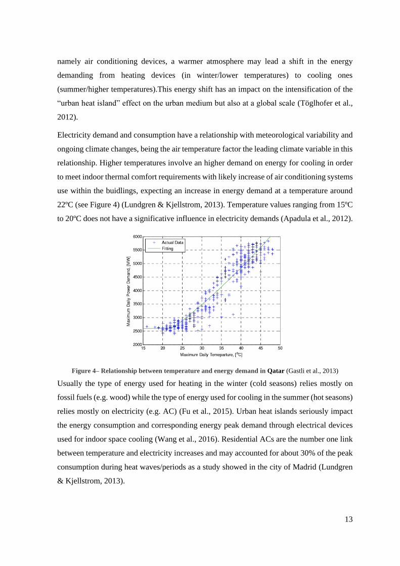
Electricity demand and consumption have a relationship with meteorological variability and

ongoing climate changes, being the air temperature factor the leading climate variable in this

relationship. Higher temperatures involve an higher demand on energy for cooling in order

to meet indoor thermal comfort requirements with likely increase of air conditioning systems

use within the buidlings, expecting an increase in energy demand at a temperature around

22ºC (see Figure 4) (Lundgren & Kjellstrom, 2013). Temperature values ranging from 15ºC

to 20ºC does not have a significative influence in electricity demands (Apadula et al., 2012).

Figure 4– Relationship between temperature and energy demand in Qatar (Gastli et al., 2013)

Usually the type of energy used for heating in the winter (cold seasons) relies mostly on

fossil fuels (e.g. wood) while the type of energy used for cooling in the summer (hot seasons)

relies mostly on electricity (e.g. AC) (Fu et al., 2015). Urban heat islands seriously impact

the energy consumption and corresponding energy peak demand through electrical devices

used for indoor space cooling (Wang et al., 2016). Residential ACs are the number one link

between temperature and electricity increases and may accounted for about 30% of the peak

consumption during heat waves/periods as a study showed in the city of Madrid (Lundgren

& Kjellstrom, 2013).

14

In order to in fact analyse the relation between excess cooling energy demand in summer

due to UHI effect, the degree-hours calculation method was used to define this relation

through the total number of cooling degree-hours (CDH) variables in linear form

(Vardoulakis et al., 2013)

𝐶𝐷𝐻 = ∑(𝑡0̅ − 𝑡𝑏𝑎𝑙)

𝑁

𝑗=1

(1)

Where, 𝑡0̅ is the hourly mean outdoor temperature of the station, tbal is the building base

temperature and N the number of hours within a month.

Cooling-degree hours give the indication of days of building cooling energy consumption

required according to the outside temperature within a month and for a specific location

where outside temperature exceeds a site specified base temperature. The building base

temperature depends on construction characteristics, use and type (Designing Buildings

wiki, n.d).

2.2 Air pollution

2.2.1 Context

Industry growth and development has been accompanied by rapid economic growth

followed by a rapid urbanization within cities with more people living in the same previous

space. This generates an increase in human activities which release a wide range of emissions

into the urban environment, causing a rise in the concentration of air pollutants in the outdoor

ambient when comparing with the rural surrounding areas and other natural ecosystems (Han

et al., 2014).

Air pollution in cities represent one of the biggest challenges of this century, posing its

exposure risks and severe implications for human health besides having a negative impact

on the environment, particular attention and concern has been given to ground level ozone

(O3) and particulate matter with an aerodynamic diameter under 10 µm (PM 10) and 2,5 µm

(PM 2.5) (Miranda et al., 2016).

15

Trees and vegetation play an important role concerning air quality, removing air pollutants

mainly through the process of dry deposition and interception of particles and the uptake of

gases by the stomata, thus reducing air pollution (Rocha et al., 2019). Vegetation can also

influence air temperature, human health and well-being and building’s energy costs among

other additional benefits (see Table 3).

16

Table 3 - Compilation of studies that prove the impact of NBS implementation on air quality and its respective co-benefits

NBS Study Area Impact Co-Benefits

Green Spaces (Rocha et al.,

2019)

Lisbon,

Portugal

Regulating

Air Quality

Microclimate Regulation; noise reduction, flood risk reduction

Green Roofs

and Living

Walls

(Viecco et al.,

2018)

Semiarid

Climates

Building’s energy savings, promoting biodiversity, controlling water run-off, mitigating

urban heat island effect

Trees (Selmi et al.,

2016)

Strasbourg,

France Recreation, cultural, aesthetic, regulation of temperature; carbon sequestration

(Nowak et al.,

2018) Canada Air temperature reductions, human health improvements

Urban Forests (Baró et al.,

2014)

Barcelona,

Spain

Global climate regulation, urban temperature regulation, noise reduction, runoff mitigation,

and recreational opportunities

17

2.2.2 Impact assessment

The health impacts of outdoor air pollution are mainly expressed in two indicators (mortality

and morbidity) derived from long-term and short-term exposure of air pollutants. Mortality

refers to non-accidental premature deaths and reduction in life expectancy; morbidity refers

to illness occurrence thus hospital admissions, years of life dealing with a disability/ year of

life with limitations due to the disease, workdays and productivity loss, etc.

The harmful impacts of outdoor air pollution in human health have been described in several

studies that link these air pollutants with respiratory and cardiovascular diseases, among

these, lung cancer, acute lower respiratory infection, strokes, ischaemic heart disease and

chronic obstructive pulmonary disease, etc. showing a relationship of outdoor air pollution

with the increase morbidity (illness/hospital admissions) and premature mortality

worldwide, being elderly people and children the most vulnerable groups to it (WHO, 2018).

Health outcomes linked to air pollution that can be noticed after short exposure periods result

in acute effects, while a long-term exposure results in chronic effects (Rafael et al., 2018).

According to OECD a prediction of premature deaths caused by outdoor air pollution

(specifically PM and ozone) is expected to triple until 2060 from 2010 values, being

significantly higher in developing countries like India and China which are have high

population density (see Figure 5) (OECD, 2016).

Figure 5- Number of premature deaths per year and per million people caused by outdoor air

pollution (particulate matter and ozone) in 2010 and its estimation for 2060 for different countries

(OECD, 2016)

18

The standard economic valuation methodology for morbidity is made based on “cost-of-

illness” (COI) approach which estimates the costs of hospital admissions and medical and

non-medical resources to treat a disease and productivity and production losses due to illness

and does not consider non market values (e.g. pain and suffering) (Silveira et al., 2015) and

for mortality, it is used the “value of a life year” (VOLY) monetary approach, (WHO, 2015).

Concentration-response functions (CRFs) linking PM10, PM2.5 and NO2 concentrations

exposure with health outcomes (morbidity and mortality indicators) at a population level

given as relative risk (RR) are recommended in the HRAPIE project for those pollutant-

outcome pairs where an evidence of an association of the pollutant with a health outcome

previously concluded in the REVIHAAP project for an impact and cost assessment of

outdoor air pollutants (PM10, PM2.5 and NO2) considering specific conditions in the EU

countries, concentrations expected by 2020 and the availability of baseline health data

(Héroux et al., 2015).

The relative risk (RR) or risk ratio is based on epidemiological studies and it is the “ratio of

the probability of an event occurring in the exposed group versus the probability of the event

occurring in the non-exposed group”, where if the risk is higher than 1 means that the risk

of the outcome is increased by the exposure and defined at population level (Tenny &

Hoffman, 2019).

The following equation (De Leeuw & Horálek, 2016) gives us the RR:

𝑹𝑹 = 𝒆𝒙𝒑[𝑩(𝑪 − 𝑪𝟎)] (2)

Where B is the concentration-response factor, C is the estimated average concentration and

C0 is the reference concentration.

The formulation for the number of unfavourable implications (Silveira et al., 2015) is given:

𝜟𝑹 = 𝑰𝑹𝒊 × 𝑪𝑹𝑭𝒊,𝒑 × 𝑪𝒑 × 𝒑𝒐𝒑 (3)

Where, 𝛥𝑅 is the the number of the unfavourable implications (cases, days or episodes) over

all health indicators (e.g. number of premature deaths, days of hospital admissions, etc.) due

to outdoor air pollution, 𝐼𝑅 is the annual baseline rate of the given health effect i (%) for

both sex groups and for all ages (assumed to be constant over the country), CRF is the

concentration-response function which is the correlation coefficient between the pollutant p

concentration variation and the probability of experiencing a specific health indicator i. The

19

CRF is related with the Relative Risk (RR) (%). For example, RR for premature mortality

due to PM2.5 exposure within people above 30 years old is 1,062 per 10 μg/m3, which means

that, assuming linearity, for an increase in 10 μg/m3 of PM2.5, the total mortality increases

by 6,2 % in the exposed population. Finally, Cp indicates the pollutant p concentration

(μg/m3) before and after the adoption of NBS, calculated using WRF-Chem and pop is the

population units exposed to the pollutant p.

The concentration-response functions (CRF) are described in Tables 4, 5 and 6 for three

outdoor air pollutants: PM10, PM2.5 and NO2 respectively, recommended from the HRAPIE

project (WHO, 2013).

20

Table 4 – Health effects related with PM10 exposure, concentration-response functions (CRF) and of respective economic valuation (base costs €2015)

Health Endpoint Age

Group

Exposure

Period

Relative Risk (95% CI) per

10µg/m3

Reference Costs

(€/unit)

Unit References

Total mortality (all-causes) < 1 year Long-term 1.04

(1.02-1.07)

90 000 (2003) VSL (WHO, 2013)

(Chiabai, Spadaro, &

Neumann, 2018)

Asthma symptoms 5 - 19

years

Short-term 1.028

(1.006-1.051)

530 (2007)

42 (2005)

Case/year

Day

(WHO, 2013)

(Maurits & Hoogenveen,

2013)

(Holland, 2014)

Chronic bronchitis (incidence) >18 years Long-term 1.117

(1.040–1.189)

53 600 (2005) Case (WHO, 2013)

(Holland, 2014)

Notes:

- VSL: value of a statistical life

21

Table 5 - Health effects related with PM2.5 exposure, concentration-response functions (CRF) and of respective economic valuation (base costs €2015)

Health Endpoint Age

Group

Exposure

Period

Relative Risk (95% CI) per

10µg/m3

Reference Costs

(€/unit)

Unit References

Total Mortality All Short-term 1.0123

(1.0045-1.0201)

90 000 (2003) YOLL (WHO, 2013)

(Chiabai et al., 2018)

HA,

Cardiovascular

diseases

All Short-term 1.0091

(1.0017–1.0166)

2220 (2005) Hospital

Admission

(WHO, 2013)

(Holland, 2014)

Notes:

- HA: hospital admissions

- YOLL: years of life lost.

Table 6 - Health effects related with NO2 exposure, concentration-response functions (CRF) and of respective economic valuation (base costs €2015)

Health Endpoint Age Group Exposure Period Relative Risk (95% CI) per 10µg/m3 Reference Costs (€/unit) Unit Reference

Mortality, all-cause (natural) All Short-term 1.0027

(1.0016–1.0038)

90 000 (2003) YOLL (WHO, 2013)

(Chiabai et al., 2018)

HA, respiratory diseases All Short-term 1.0180

(1.0115–1.0245)

2220 (2005) Case (WHO, 2013)

(Holland, 2014)

Notes:

- HA: hospital admissions.

- YOLL: years of life

22

2.3 Urban flooding

2.3.1 Context

The frequency and magnitude of flood events is expected to increase due to the effects of

climate change, socio-economic key drivers, land-use change patterns, and soil sealing

(Svetlana et al., 2015). One of the characteristics associated with urbanization is the

conversion of pervious terrain into impervious surfaces to accommodate the urban expansion

and development, causing a reduction in the natural system to infiltrate water which results

in an increase of surface runoff (Brody et al., 2007). Frequently engineered solutions, such

as dredging or diverting natural streams, are thought to mitigate flood effects. In most cities

the conventional method to address excess water is to convey the water away from the city

area, in the shortest time possible, through a conduit-based drainage system and discharge it

to the nearest stream resulting in increasing flood peaks and a smaller groundwater recharge

(Lashford, 2016).

Instead of moving the problem and possibly creating floods downstream, Sustainable Urban

Drainage Systems (SuDS) - a concept enclosed by NBS - focus on recreating the natural

hydrological conditions and thus re-establish the natural infiltration capacity of the soil and

boosting groundwater recharge. Usually it is implemented using green solutions such as

vegetation or permeable areas. Some examples of SuDS may include green roofs, retention

basins and bioretention ponds, which provide areas for water to be stored and infiltrate into

the soil and also allows that the water be either evaporated or transpired by vegetation

(evapotranspiration) (Lashford, 2016). Besides providing a water storage and thus reducing

the flood risk and peak runoff flow, these infrastructures also ensure other benefits such as

enhancing water quality, temperature regulation, environment aesthetics and habitat for

wildlife (see Table 7).

23

Table 7 - Examples of studies that quantify the impact of NBS implementation on flood risk and its respective co-benefits

NBS Study Area Impact Co-Benefits

Combined urban

parks and retention

basins

(Roebeling et al.,

2011)

Aveiro

(Portugal)

Flood risk

reduction

Appreciation of real estate values

“Sponge City”

Concept (Chan et al., 2018) China

Enhancement of ecological functions; aesthetics benefits; Additional Amenity space;

urban water body preservation; storage, infiltration and purification of stormwater; grey-

water reuse

Green Roof-Trees

Combination (Zölch et al., 2017)

Munich,

Germany

Sequestering and storing carbon emissions, biodiversity benefits by providing habitat,

and social and health benefits by providing areas of recreation filtering air pollutants and

reducing noise pollution

SuDS combination (Lashford, 2016)

Leicester,

United

Kingdom

Carbon sequestration, urban cooling, and energy reduction, water quality increasing

24

2.3.2 Impact Assessment

Flood damage can be divided in tangible and intangible damage. The first one is directly

evaluated in monetary terms, while the latter cannot be assessed in monetary terms (Romali

& Sulaiman, 2015). Tangible damage can also be divided in direct damage caused by the

contact or submersion in water (destruction of infrastructures like buildings, roads and

railroads for example) and indirect damage caused by the interruption of physical and

economic networks (disruption of public services, business interruption on the flooded area,

damage to livestock, etc). Intangible damage refers to assets that do not possess a market

value such as injuries, trauma, loss of life, phycological distress, etc. (Merz et al., 2010).

Assessing the expected damage caused by flood events is conventionally done using

damage-functions, by considering the relation between floodwater depth and percent damage

for a variety of sectors. This methodology represents the economic loss (as absolute or

relative values) as a function of the maximum water depth. Nonetheless other factors may

influence the amount of damage caused by a flood event such as flow velocity, duration of

flood, effectiveness of the emergency response, etc. (Middelmann-Fernandes, 2010). A

common approach is to define the damage percentage as “the ratio of the total cost to replace

the damaged components of a flood-affected property to the pre-disaster market value of the

property” and with the costs of the repair and the market value referring to the same period

(Pistrika et al., 2014). Figure 6 shows an example of the depth damage curve for the German

economy. With an increase of population and services localised in vulnerable flood risk

areas, the damage on infrastructure might increase and consequently the related costs will

be higher (Svetlana et al., 2015).

Figure 6- Depth Damage function for the different sectors in Germany’s economy (Prahl et al., 2018)

25

2.4 Sprawl, gentrification and real estate valuation

The migration of the population for sub-urban, undeveloped and peripherical areas

(exponentiated by urban population and economic growth and limited available area within

the city) with low-density dwellings and segregated land-use creates a process of urban

sprawl. This type of population distribution leads to a conversion of natural and agriculture

areas for mainly residential and commercial sector construction, resulting in cities’

expansion. Urban sprawl comes along with problems at social and economic levels, among

them: non-efficient use of resources, less transportation alternatives (private transportation

dependency), loss of biodiversity, etc. (Broitman & Koomen, 2015; Haaland & van den

Bosch, 2015).

The urbanization phenomenon and cities’ expansion lead decision-makers and planners to

make policies to adapt cities to these changes, often requiring the conversion of green

infrastructure into residential and commercial properties to accommodate and make room

for the increasing population (Mayor et al., 2009; Poudyal et al., 2009; Kabisch & Haase,

2014; Roebeling et al., 2017). These urbanization changes leave the remaining green open

spaces to be shared by a growing number of residents, being the existing available areas

insufficient to respond and supply the necessary benefits and recreational potential to its

users. The loss, intensive use and degradation of these spaces may have an undesirable and

opposite effect to its users (Poudyal et al., 2009).

The lack of a reasonable amount of green/blue spaces in cities makes them more valuable

for residents that recognise their recreational, aesthetic and physical benefits (Mayor et al.,

2009; Xiaoyun, 2015). There is a supply-demand shift in the real estate market linked to the

deficiency of a fair availability and quality of green areas within the urban medium.

Although many studies prove the health and well-being benefits of green/blue urban areas

(besides the environmental amenities) there is still a challenge to properly quantify them in

monetary gains since the access to these spaces is usually free. In order to provide its value,

a non-market method is usually used – the hedonic pricing method.

26

The hedonic pricing method decomposes the total price of a good in the monetary value of

each one of the characteristics/benefits that comprises that good. The price of a house can

be divided into its attributes: number of rooms, age of the building, garage space, living area,

etc. Besides its physical characteristics, neighbourhood and surrounding characteristics have

also a significative weight for homebuyers when it comes to choosing a property: distance

to work, proximity to schools, hospitals, public transportation/ road access availability,

proximity to environmental amenities, etc. (Morancho, 2003; Mayor et al., 2009; Roebeling

et al., 2017). From all the factors that can influence housing preference and thus the prices

and real estate market, environmental amenities pose as one of the top (Trojanek et al., 2018).

Using regression techniques, the method can identify the fraction attributable to

environmental amenities (green/blue spaces).

As the competition and demand for these attractive areas rise, so does the real estate values,

and property values may boost from 6-8% in the Netherlands, to 17% in China and 20% in

the USA when close to parks (ATCC, 2014), leading to environmental gentrification in

which higher income households are mainly benefited, accentuating the income inequalities

within a city, and displacing lower income households, resulting in a change in demographic

distribution patterns. With an increased added value of environmental amenities of

green/blue spaces, households with a higher purchasing power are willing to pay more for

less living space when living close to these type of areas. (Roebeling et al., 2017; Augusto,

2018). Several studies show that housing market prices are influenced by proximity, size and

view of this areas, being proximity the most significative and impactful factor (Mayor et al.,

2009; Lin et al., 2015).

Green/blue spaces (e.g. parks, ponds, lakes, etc.) as well as the integration of greenery and

vegetation on buildings (green roofs/green façades/green walls) in the urban medium

represent a solution to promote urban densification in build-up central areas, as it will create

a favourable, attractive, recreational, aesthetically beautiful and restorative local

environment (ATCC, 2014; Roebeling et al., 2017). Moreover, it provides important

ecosystem services like carbon sequestration, temperature regulation and noise pollution

reduction (see Table 8), adding not only value to the house itself but also to the urban

environment, creating natural and green landscapes.

27

Table 8 - Compilation of studies that prove the impact of NBS implementation on urban densification and its respective co-benefits

NBS Study Area Impact Co-Benefits

Urban Forest (Tyrväinen, 1997)

North

Carelia

(Finland)

Real estate

valuation

Balanced microclimate; pleasant landscape, clear air, peace and quiet,

recreation, improved aesthetics; erosion control

Urban Green

Spaces (Trojanek et al., 2018)

Warsaw

(Poland)

Human health and wellbeing, social cohesion, tourism, biodiversity, air

quality improvement and carbon sequestration, water management, cooling of

urban areas.

Urban Green

Spaces (Morancho, 2003)

Castellón

(Spain)

Carbon sequestration; regulation of humidity; temperature and rainfall, soil

erosion restraining; form the basis for the conservation of fauna and flora

Urban Green

Spaces

(Kolbe & Wüstemann,

2014)

Cologne

(Germany)

Recreational and aesthetic benefits; carbon sequestration and storage;

wellbeing; biodiversity and habitats protection;

28

3.Methodology

In this Section an economic evaluation is performed for the different endpoints (flood depth

and real estate values) in each of the urban challenges ( flood risk and urban sprawl) for the

quantification of the external costs building on the Impact Pathway Approach (IPA; Merz et

al., 2010; Silveira et al., 2015; see Figure 7). This approach has several steps: i) quantifying

the impact in terms of influencing factors (precipitation and urbanization), for this part an

environmental assessment is performed in which the several disciplinary models described

in this study are used (see Section 3.1), ii) linking the influencing factors with a bio-physical

impact (damaged buildings and changes in the real estate market) based on literature (i.e.

exposure-response functions); and iii) attributing a monetary value to the answer about the

corresponding impact (see Section 3.2).

Figure 7 - Schematic Representation of the Impact Pathway Approach (adapted)

In this study the focus will be on flood risk mitigation and sprawl, gentrification and real

estate valuation. Urban heating and air pollution were not considered as there was a lack of

information on temperature and air pollution (PM10, PM2.5 and NO2) at a spatial scale (1km

* 1km) relevant for this study.

29

3.1 Environmental assessment

In this section we described the models (InfoWORKS, Section 3.1.1; SULD, Section 3.1.2)

used in this study to assess the changes in environmental states (flood risk; sprawl,

gentrification and real estate valuation) due to the implementation of NBS.

3.1.1 InfoWORKS

This section describes the InfoWORKS ICM (Integrated Catchment Management) model

used to assess the impacts of NBS implementation on urban flood adaptation.

Included in the pre-processing is the calculation of synthetic hyetographs to be used as an

input to the model. Instead of the traditional IDF curves (Intensity-duration-frequency

curves) were used DDF curves (Depth-duration-frequency curves), which relates the rainfall

depth with the duration and frequency of occurrence.

InfoWORKS ICM will model rainfall, surface and subsurface processes separately for the

sub-catchments comprising therefore three major steps. The first step is the calculation of

surface runoff conveyed into the pipes. This is done using the Unit hydrograph model and

the Desbordes time of concentration (Desbordes, 1978). The second step is running the

hydraulic model inside the pipes and conveying the flow using Mass and Momentum

conservation equations such as Saint Venant. The third step is the calculation of 2D flow

and the interaction between the surface and sub-surface model when the conduits surcharge

using the 2D model MULFLOOD (Innovyze, 2018).

InfoWORKS ICM (Innovyze, 2018) model comprises two models and the linkage between

both: a sub-surface network (1D model), an overland surface network (2D model) and the

interaction between sub-surface and surface flow (1D/2D linkage).

1D sub-surface flow model

The sub-surface network flood wave can be described by solving the 1D Saint-Venant

equations in the pipe network:

𝜕

𝜕𝑡𝐴 +

𝜕

𝜕𝑥𝑄 = 0

(4)

30

𝜕

𝜕𝑡𝑄 +

𝜕

𝜕𝑥

𝑄2

𝐴+ 𝑔𝐴 (cos 𝜃

𝜕𝑦

𝜕𝑥− 𝑆0 +

𝑄|𝑄|

𝐾2) = 0 (5)

where 𝑄 is the discharge (m3/s), A is the cross-sectional area (m2), 𝑔 is the acceleration due

to gravity (m/s2),𝜃 is the angle of bed to horizontal (degrees),𝑆0 is the bed slope and K is

conveyance.

These equations are solved implicitly using the Preissmann four-point scheme, in which

functions and derivatives are replaced by weighted averages over the four corners of a box

in (x,t) space.

2D surface flow model

The 2D surface flood wave can be described by the Shallow Water Equations:

𝜕

𝜕𝑡ℎ +

𝜕

𝜕𝑥(𝑢ℎ) +

𝜕

𝜕𝑦(𝑣ℎ) = ∑ 𝑞𝑖

𝑛

𝑖=1

(6)

𝜕

𝜕𝑡𝑢ℎ +

𝜕

𝜕𝑥𝑢2ℎ +

1

2

𝜕

𝜕𝑥𝑔ℎ2 +

𝜕

𝜕𝑦𝑢𝑣ℎ

= −𝑔ℎ𝜕

𝜕𝑥𝐵 − 𝜏𝑏𝑥 + ∑ 𝑞𝑖𝑢𝑖

𝑛

𝑖=1

(7)

𝜕

𝜕𝑡𝑣ℎ +

𝜕

𝜕𝑥𝑢𝑣ℎ +

𝜕

𝜕𝑦𝑣2ℎ +

1

2

𝜕

𝜕𝑦𝑔ℎ2 = −𝑔ℎ

𝜕

𝜕𝑦𝐵 − 𝜏𝑏𝑦 + ∑ 𝑞𝑖𝑣𝑖

𝑛

𝑖=1

(8)

Equation 6 is the mass conservation equation and Equations 7 and 8 are the two momentum

conservation equations. Where h represents the water depth, u and v the velocity components

in the x and y orthogonal directions respectively, qi is the i th net source discharge per area ,

ui and vi are the velocities in the x and y directions of the ith net source discharge,

respectively, g is the gravitational acceleration, B is the bed elevation and n the Manning’s

Roughness coefficient.

1D/2D interaction

The sub-surface system (conduits and manholes) becomes surcharged and the pipes become

completely full due to a rainfall event posing a pressure increase in the pipe network thus

31

forcing water to flow out from the drainage system through manholes to the surface system

(streets) - pressurized flow (see Figure 8) .

Figure 8 – “Preissmann Slot”- conceptual vertical and narrow slot providing a conceptual free surface

condition for the flow when the water level is above the top of a closed conduit

The overflow running out from manholes (linkage element) causing street flooding uses

vertical Weir/Orifice Equation in order to determine the exchange flow between the sewer

and surface network.

The data applied to the model is acquired through stakeholders and open source databases:

precipitation patterns through time, historical floods, physical characteristics of the city,

streams/water bodies nearby, NBS to be applied to the case study, etc. InfoWORKS ICM

(Innovyze, 2018) model simulations results are available in the form of tables and maps,

graphs, raw data, GIS compatible formats or images. Depth-damage curves will be applied

to the outputs obtained from the 1D/2D interaction in order to allow subsequently assess the

flood damage by sector (residential, infrastructure, commercial, etc.) and in total.

3.1.2 SULD

This section describes the Sustainable Urbanizing Landscape Development (SULD) model

developed by Roebeling et al. (2017) used in this study to assess the impacts of NBS

implementation on urban densification adaptation.

This decision support tool is an economic and hedonic pricing simulation, spatially explicit

Geographic Information System (GIS) based model that helps and provides information for

stakeholders in the decision-making process regarding a sustainable urban and peri-urban

planning, development and management including environmental amenities (green/blue

32

spaces) through the application of the hedonic pricing simulation method (Roebeling et al.,

2017). The hedonic price method determines housing location choices and decomposes the

total value of the house into every constituent that has a contribution for its price, linking the

building value and structural characteristics (number of rooms, number of bathrooms, size,

age, garage space, etc.) with the surrounding characteristics of the neighbourhood/ amenities

characteristics (location, proximity to the city centre, access to transportation, proximity to

environmental amenities, dimension and views or access to the green space, less noise

spaces) (Mayor et al., 2009).

In this study the model will be used to determine the impact and influence of location-

specific environmental amenities (aesthetics, recreational, etc.) on house prices for the city

centre of Eindhoven, Netherlands.

The demand side (Equation 9) is represented by households, considering their preferences

regarding certain goods and services, as residential space S, other goods and services Z, and

environmental amenities 𝑒. The utility obtained by households in each location depends on

their preferences, distance to environmental amenities and income y. Hence, households aim

to maximize their utility 𝑈 at a certain location 𝑖, subject to the budget constraint y, that is

spent on housing (𝑝𝑖ℎ𝑆𝑖 ), other goods and services (𝑍), and transportation between the

residential area and the urban centre (𝑝𝑥𝑥𝑖):

max𝑆𝑖,𝑍𝑖

𝑈𝑖(𝑆𝑖, 𝑍𝑖) = 𝑆𝑖𝜇

𝑍𝑖1−𝜇

𝑒𝑖𝜀 𝑠𝑢𝑏𝑗𝑒𝑐𝑡 𝑡𝑜: 𝑦 = 𝑝𝑖

ℎ𝑆𝑖 + 𝑍𝑖 + 𝑝𝑥𝑥𝑖 (9)

where 𝑝𝑖ℎ is the rental price of housing (€/m2), 𝑝𝑥 the commuting cost (€/km) and 𝑥𝑖 the

road-network distance to the closest urban centre (km). Moreover, 𝜇 is the elasticity of

demand for residential space ( 𝑆𝑖 ) and 𝜀 is the elasticity of utility with respect to

environmental amenities (𝑒𝑖). The household’s bid-rent price for housing 𝑝𝑖ℎ∗ (maximum

household willingness to pay for housing at location i – demand side of the real estate

market) which optimized their residential location by trading off trading off utility from

environmental amenities (𝑒𝑖), residential space ( 𝑆𝑖) and other goods and services (𝑍𝑖) versus

land rent (𝑝𝑖ℎ𝑆𝑖) and commuting costs (𝑝𝑥𝑥𝑖), subject to a budget constraint (y) and is now

given by:

33

𝑝𝑖ℎ∗ = (

𝜇𝜇(1 − 𝜇)1−𝜇𝑒𝑖𝜀(𝑦 − 𝑝𝑥𝑥𝑖)

𝑢)

1𝜇

(10)

where 𝑢 is the utility level 𝑈.

The supply side (Equation 11) is represented by real estate developers which aim to

maximize their profit (𝜋) at location i by trading off returns from housing construction

revenue(phD) and associated development costs (l+Dη), that are subject to households’

willingness to pay for housing:

max𝐷𝑖

𝜋𝑖(𝐷𝑖) = 𝑝𝑖ℎ𝐷𝑖 − (𝑙𝑖 + 𝐷𝑖

𝜂) 𝑤𝑖𝑡ℎ: 𝐷𝑖 = 𝑛𝑖𝑆𝑖 (11)

where 𝑝𝑖ℎ is the rental price of housing, 𝑙𝑖 the opportunity cost of land, 𝐷𝑖

𝜂 the construction

cost function (with 𝜂 the ratio of housing value to non-construction costs), 𝑛𝑖 the household

density and 𝑆𝑖 the residential space. The developer’s bid-price for land 𝑟𝑖∗∗ is now given by:

𝑟𝑖∗∗ = (𝑚𝑝𝑖

ℎ∗∗)𝜂

𝜂−1 (12)

where 𝑚 = [(𝜂 − 1)𝜂−1 𝜂⁄ ] 𝜂⁄ . This equation determines the minimum rental price for

housing the developer is willing to accept (𝑝𝑖ℎ∗∗), thus representing the supply side of the

housing market. This means that developers will only develop when residential land rents

(𝑝𝑖ℎ𝐷𝑖) are larger than the opportunity cost of development (𝑙𝑖 + 𝐷𝑖

𝜂), which corresponds to

the foregone land rents (𝑙𝑖) and investments in land conversion (𝐷𝑖𝜂).

The equilibrium is where the housing supply equals the demand (i.e. 𝑝𝑖ℎ∗ = 𝑝𝑖

ℎ∗∗). The land

rent price 𝑟𝑖 can now be derived using Eq. 10 and 11, and is given by:

𝑟𝑖 = (𝑘𝑒𝑖

𝜀(𝑦 − 𝑝𝑥𝑥𝑖)

𝑢)

𝜂 𝜇(𝜂−1)

(13)

where 𝑘 = 𝜇𝑚𝜇(1 − 𝜇)1−𝜇. The corresponding optimal household density 𝑛𝑖 is given by:

𝑛𝑖 =𝐷𝑖

𝑆𝑖

(14)

34

with 𝑆𝑖 = 𝜇(𝑦 − 𝑝𝑥𝑥𝑖) 𝑝𝑖ℎ𝑥⁄ the necessary condition for optimality 𝑈𝑖 and with 𝐷𝑖 =

(𝜂 − 1)1 𝑛⁄ (𝑟𝑖)1 𝑛⁄ the necessary condition for optimality of 𝜋𝑖, and where 𝑝𝑖

ℎ∗ and 𝑟𝑖 are

given in Equations (10) and (13), respectively.

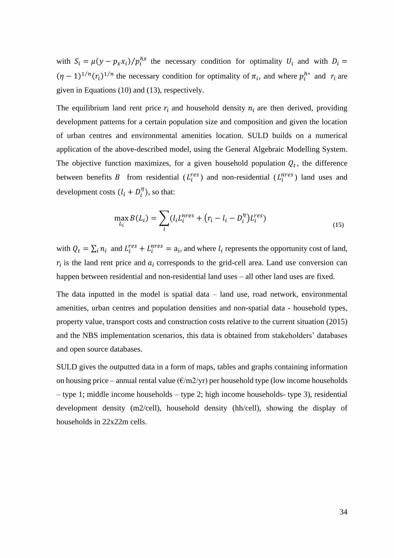
The equilibrium land rent price 𝑟𝑖 and household density 𝑛𝑖 are then derived, providing

development patterns for a certain population size and composition and given the location

of urban centres and environmental amenities location. SULD builds on a numerical

application of the above-described model, using the General Algebraic Modelling System.

The objective function maximizes, for a given household population 𝑄𝑡 , the difference

between benefits 𝐵 from residential (𝐿𝑖𝑟𝑒𝑠 ) and non-residential ( 𝐿𝑖

𝑛𝑟𝑒𝑠 ) land uses and

development costs (𝑙𝑖 + 𝐷𝑖𝜂

), so that:

max𝐿𝑖

𝐵(𝐿𝑖) = ∑(𝑙𝑖𝐿𝑖𝑛𝑟𝑒𝑠 + (𝑟𝑖 − 𝑙𝑖 − 𝐷𝑖

𝜂)𝐿𝑖

𝑟𝑒𝑠)

𝑖

(15)

with 𝑄𝑡 = ∑ 𝑛𝑖𝑖 and 𝐿𝑖𝑟𝑒𝑠 + 𝐿𝑖

𝑛𝑟𝑒𝑠 = ai, and where 𝑙𝑖 represents the opportunity cost of land,

𝑟𝑖 is the land rent price and 𝑎𝑖 corresponds to the grid-cell area. Land use conversion can

happen between residential and non-residential land uses – all other land uses are fixed.

The data inputted in the model is spatial data – land use, road network, environmental

amenities, urban centres and population densities and non-spatial data - household types,

property value, transport costs and construction costs relative to the current situation (2015)

and the NBS implementation scenarios, this data is obtained from stakeholders’ databases

and open source databases.

SULD gives the outputted data in a form of maps, tables and graphs containing information

on housing price – annual rental value (€/m2/yr) per household type (low income households

– type 1; middle income households – type 2; high income households- type 3), residential

development density (m2/cell), household density (hh/cell), showing the display of

households in 22x22m cells.

35

3.2 Compilation and synthesis of the relationship between

physical and economic impacts

Compilation of data and information (based on literature and report review) for the

development of damage-functions as well as associated cost and willingness-to-pay

functions and connecting the alterations (i.e. precipitation) and the physical impacts (i.e.

damage to buildings) and, at last, to its economic impact (cost). This will result in generic

dose-cost and depth-damage functions that can be used to determine the impacts, costs

and/or benefits related to the baseline and NBS scenarios.

The urban flooding will be quantified in terms of flood depth damage on several sectors

(residential, agriculture, commerce, etc.) and its corresponding economic valuation. In this

study we will only consider one of the parameters to assess the flood damage, which is the

flood water depth, being this not only the most important in cost estimation studies but also

the easier to quantify and the one that causes greater damages (main factor of direct damage)

(Genovese, 2006).

The depth damage curves are a common methodology used to calculate flood damage and

are a function of: i) the different type of land uses (damaged sector) coupled with the

orography of the city, ii) flood depth , iii) damaged fraction of the and iv) monetary value

per unit of area. The generic formulation is:

𝐷𝑎𝑚𝑎𝑔𝑒 (€) = 𝐴 × 𝑑𝑓 × 𝑃 (16)

Where A is the area (m2) of the corresponding land use, df is the water depth damage factor

(as a function of the flood depth and the damaged fraction) and P is the average price or

value per m2. All prices and values are given in Euros for the year 2015.

The depth damage curves are usually presented as a set of points rather than an expression.

These curves were converted to functions by fitting a third-degree polynomial. The

maximum depth is usually an established depth for which the building might suffer

catastrophically failure and therefore considered totally lost. These values are usually

systematically obtained from regression analysis of damage values identified in literature

(Huizinga et al., 2017). For built-up areas the land use class is expressed per unit area (land-

use based).

36

Residential buildings

An average of the local values for housing prices (€/m2/year) within the study area provided

by SULD (baseline scenario) were converted to their total real estate value (€/m2)

(considering an interest rate of 5%). The maximum damage values for the residential sector

are based on full construction costs, referring to building’s structural costs. The damage

percentage for each flood depth is bellow represented in Figure 9. The damage for the

residential sector was 1301€/m2.

Figure 9 – Percentage of damage for residential buildings according to flood depth

Commercial and Industrial buildings

For commercial and industrial buildings an average of values provided by (Huizinga et al.,

2017) was calculated, since the GIS file obtained has these two sectors aggregated. The

values used were land-used based, since there is not enough information in order to do the

calculations building-based (with structural and content damages). The values obtained

€2010 were converted into €2015 values using consumer price index (CPI) from World Bank

(https://data.worldbank.org). The damage percentage associated with flood depth is

represented in Figure 10. The maximum damage for commercial and industrial buildings

was 380 (€2015/ m2).

y = 0,0065x3 - 0,0869x2 + 0,457xR² = 0,9956

0,00

0,10

0,20

0,30

0,40

0,50

0,60

0,70

0,80

0,90

1,00

0 1 2 3 4 5 6 7

Dam

age

fact

or

Flood depth (m)

37

Figure 10 - Percentage of damage for commercial and industrial buildings according to flood depth

Infrastructure (roads)

The calculation procedure for infrastructure damage was the same as described for

commercial and industrial damage. The damage percentage associated with flood depth is

bellow represented in Figure 11. The maximum damage for infrastructure was 32 (€2015/

m2).

Figure 11 - Percentage of damage for infrastructure according to flood depth

y = -0,0011x3 - 0,0162x2 + 0,3034xR² = 0,9992

0,00

0,10

0,20

0,30

0,40

0,50

0,60

0,70

0,80

0,90

1,00

0 1 2 3 4 5 6 7

Dam

age

fact

or

Flood depth (m)

y = 0,0058x3 - 0,0871x2 + 0,4829xR² = 0,9963

0,00

0,10

0,20

0,30

0,40

0,50

0,60

0,70

0,80

0,90

1,00

0 1 2 3 4 5 6 7

Dam

age

fact

or

Flood depth (m)

38

4. Case study description

4.1 Eindhoven

The case study area is the city of Eindhoven, the fifth largest city in the Netherlands, located

in the south-east part of the country in the province of North Brabant, close to the Belgian

and German borders of the Netherlands with a population of about 224 900 inhabitants in

2015 and an area of approximately 78 km2 (Population.City ,n.d), thus an average population

density of 2883 inhabitants/km2. The city was originally located in the confluence of the

Dommel and Gender streams, nowadays the Gender is covered and invisible in the city

centre, however the Dommel stills flow through the city openly (Zetcijen, 2016).

In 1890 Philips Company settled in the city and was the main responsible for the industrial

development (largely dependent on fossil fuels) and demographic growth, influencing not

only the economy but also the social part of the society, having the city grown over the years

from an agriculture region to a technological and modern one we know today with a build-

up area mainly of residential and commercial character. In 1920 Eindhoven was merged with

the 5 surrounding villages Stratum, Strijp, Woensel, Tongelre and Gestel, growing from

8,000 to 45,000 inhabitants, separating these parts with green infrastructure, remaining to

this day. During Philips expansion and peak, Eindhoven population grew to 100,000

inhabitants in 1930 (Zumelzu Scheel et al., 2015; UnaLab, 2016).

The expected tendency these days is that the population continues to increase rapidly within

the next years (see Figure 12), having experienced a growth of about 13000 inhabitants from

2006 to 2015 (Zetcijen, 2016) and possibly growing to an estimated 300 000 inhabitants by

2030 (UNaLab, 2016).

39

Figure 12 - Population trend in Eindhoven

The Eindhoven case study focusses on the inner-ring of the city of Eindhoven, which

comprises 23 neighbourhoods, serviced by 4 highways, an international airport and 21

environmental amenities among them parks and water canals and ponds (UNaLab, 2016).

As many other cities in the world Eindhoven is facing urbanization and climate change

challenges, with Eindhoven focus on flooding problems and urban sprawl. With

groundwaters just below the surface most of the year and with mainly loam and loamy sand

soil which makes it harder for rainwater to quickly infiltrate in some places making flooding

problems the main challenge to deal with in the city (UNaLab, 2016).

The current land use in Eindhoven is mainly residential and industrial/commerce buildings,

with some agriculture areas in the periphery and urban parks surrounding the city centre (see

Figure 13).

Figure 13 - Land Use for the inner-ring of Eindhoven

40

4.2 Scenario description

Several scenarios will be applied to the SDST for the year 2015 without (Baseline scenario)

and with NBS implementation for the study area.

4.2.1 NBS scenario

The scenarios simulated for this case study were the same as the ones implemented in the

work of Bodilis (2018) and Augusto (2018) and are geographically represented (see Figure

14) and described below (see Table 10).

Figure 14 - Multiple NBS implementation scenarios in the city centre of Eindhoven, Netherlands

41

Table 9 - Description of the NBS implementation scenarios

NBS Type of NBS Description infoWORKS SULD

1 River Daylighting +

Green Space

Implementation the daylighting of a section of the Gender river, restoring it to its previous natural

condition, with the addition of a green space surrounding it.

2 River Daylighting

Gender river daylighting on the Frederika van Pruisenweg street

3 Requalification of

Green Spaces

Improving ecological status of the Gendervijver pond and enhancing the environmental amenities

of the park

4 River Daylighting

Daylighting of the Gender river near the train station (Stationsweg)

5 River Daylighting

Daylighting of the Gender river on Willemstraat

6-15 De-paving

Removing of impervious surfaces like asphalt and concrete ones and the replacement by new

permeable ones (vegetated surfaces) that allow water infiltration and creating new useful and

pleasant ones (e.g. bicycle lanes)

5. Results and discussion

By implementing the methodology and data derived from the disciplinary models mentioned

in Section 3 and the scenarios described in Section 4 for Eindhoven, results presented in the

following section are obtained in a form of risk maps and/or tables.

The SDST integrates data and information from different disciplinary models into a spatially

explicit system at the landscape scale, to assess the impacts, costs and (co-) benefits of NBS

on urban flooding and real estate market. Urban flooding is assessed using InfoWORKS

ICM model and the real estate market is assessed using SULD model (see Section 3).

Information and data are applied in the different disciplinary models a priori as well as the

baseline and NBS implementation scenarios and will integrate the systemic decision tool

(SDST) for the case study of the city of Eindhoven (Netherlands). The SDST will generate

detailed scenario simulation results for each of the physical impacts (such as exposed

population, flooded areas and affected elements) without (baseline scenario) and with NBS

implementation (see Section 4.2).

5.1 Flooding

The baseline scenario for the current situation (2015) shows a situation of flooding areas for

a return period of 20 years (1 in every 20 years flood). The flooding areas in this case study

are mainly roads since the model simulates the overcharged manholes, being the floods

originated from it.

Four main flooding areas (see Figure 15) were identified for the city centre of Eindhoven.

Figure 15 – Current situation (2015) – flood depth in Eindhoven (city centre) for a rain event of return

period of 20 years where the main flood areas are highlighted

Using the QGIS field calculator it was possible to calculate the damage (€) through the

Equations integrating the several polynomial regressions for each damage sector (see Section

3.3.3) – continuous and discontinuous urban fabric (residential area), commercial and

industrial areas and infrastructure (roads), for both baseline and NBS scenarios by creating

a conditional statement for the flood damage calculation (see Figure 16).

Figure 16 - Creation of a conditional statement in QGIS field calculator for flood damage calculation

After that by installing the module “Dissolve with stats” in QGIS it was possible to calculate

the summation of the damage (€) for each of the sectors. The costs are represented in Table

10 by sector for each scenario and in total.

Table 10- Flood damage costs for a return period of 20 years: Baseline and NBS implementation scenario

for Eindhoven (2015)

Sector Costs Baseline (€) Costs NBS (€)

Residential

Continuous urban fabric 7 601 253.3 7 311 604.9

Discontinuous urban fabric 1 535 063.3 1 422 602.1

Infrastructure (roads) 367 042.3 349 901.6

Commercial and Industrial 973 541.3 844 274.1

Total costs 10 476 900.2 9 928 382.7

Total annual costs (M€/yr) 523 845.0 496 419.1

The costs in Table 10 are being represented for a flood with a 20-year return period, which

makes them seem significantly higher than what they are when compared to the annual costs

associated to it, so the representation of the annual costs of the damages associated with the

mentioned flood gives a better understanding and perspective of the costs. Since there is only

a return period simulation, the annual costs are calculated dividing the total by 20 years.

Applying the baseline and NBS shapefile on Google Earth it was possible to do the spatial

observation of the flood range in each of the scenarios (Figure 17; see Annex II).

Figure 17 - Baseline (blue) and NBS (green) flood streams in a part of the city

Later a spatial distribution of the different types of NBS in Google Earth allow the linkage

of the impact with the NBS type (Figure 18).

Figure 18 – NBS spatial distribution with the main flood mitigation areas identified

The higher impacts produced by the different NBSs are marked in Figure 18: black line

identify the areas where there was an impact caused by the de-paving; blue lines identify the

daylighting of the river; yellow lines identify both.

Most of the initial runoff in the baseline scenario is attenuated by the de-paved areas

implementation. These high porosity permeable pavements allows rainwater to infiltrate and

be naturally stored, releasing it into the drainage system at a slower pass than a conventional

pavement (non-porous), thus reducing the runoff volume and peak discharges (Gonçalves et

al., 2017). Even though after a long period it is prone to clog due to debris and litter, thus

reducing its efficiency.

The river daylighting also plays a big part in the reduction of the flood stream. The

previously buried channel provides additional storage of the excess water volume during

rainfall events helping reduce the runoff volume which in the baseline scenario relied mostly

on the drainage system capacity which was not enough to deal with the current needs.

However, the section now open may, in a situation of an extreme rainfall to overflow,

increasing the flooded area comparing with the baseline scenario in which the excess water

was accounted only for the surcharged manholes.

Through the observation of Figure 17 and Figure 18 it is possible to conclude that the flooded

area is smaller in the NBS implementation scenario than in the baseline one, hence it’s

associated costs (Table 10).

Generally NBS show a higher efficiency when used as short-term measures (for events up

to 10-years return period) (Sörensen, 2018), unless there is a significantly large area covered

by them that can contribute for a sufficient water storage capacity (Zölch et al., 2017). When

it comes to economic benefits its more convenient to mitigate small intensity- high frequency

flooding events than high-intensity-small frequency ones, even though the last ones pose a

higher risk (Borges Batista, 2013). Since our analysis return period is higher (20-years return

period), the suggested NBS may have a high efficiency on short-term, although in a long-

term period fail to cope efficiently with high-intensity floods.

5.2 Sprawl, gentrification and real estate valuation

The results obtained from SULD for the inner ring of the city were observed using Tableau,

making possible an analysis of how NBS implementation influenced population dynamics

and the real estate market. Figure 19 shows the household density changes after the NBS

implementation, screening a significative household density decrease in the peripherical

areas of the city – outside the inner-ring (decrease from -1.43 household/cell to -1.75

household /cell) and, in turn a significative increase in the central part (increase from +0.04

household /cell to +0.48 household /cell) close to where the different NBS scenarios were

implemented.

Figure 19 - Difference between NBS and baseline scenario for household density (scenario 1-5)

Despite the remarkable household increase near the NBS scenarios implementation location,

some disperse decreasing in household density points are also present within the central area

of Eindhoven, been probably attributed to gentrification and displacement of poorer

households due to price rise in the properties in more attractive areas along with the re-

location of high-income households to near these areas (Roebeling et al., 2017; Augusto,

2018).

Likewise, the distance to largest and more attractive green/blue spaces (scenarios 1, 2 and 3)

(see Figure 20) was smaller (decrease of 8.4m to 64.7m), followed by a housing price and

real estate market rise (increase of 10.7€/m2 to 109.1€/m2) (see Figure 21) in the area. When

keeping all the properties characteristics constant, households are willing to pay up to 2.9%

more for an equivalent property when this is situated near an environmental amenity.

Households with different income and purchase power levels make this price increase lead

to an environmental gentrification process in which higher income households are benefited

over lower income households, which are taken to peripherical areas, accentuating the

income inequalities within a city (Xiaoyun, 2015).

The higher difference in prices is shown in the Witte Dame Neighbourhood, where the

scenario 1 was implemented, consisting in the daylighting of a section of Gender river and

a new park creation in the city centre.

Figure 20 - Difference between NBS and baseline scenario for distance to higher value green/blue

spaces (m)

Figure 21 - Difference between NBS and baseline scenario for house price (€/m2)

Through SULD it was possible to calculate the housing price (€) attending the square meters

in the residential sector for each grill cell (22x22m) for the inner ring of Eindhoven, both for

the baseline and NBS scenario (see Table 11).

Table 11- Real estate: annual rental value (M€/yr) for baseline and NBS implementation scenario for

Eindhoven

Baseline NBS

Housing prices (M€/yr) 205.3 211.3

The results are in line with Xiaoyun (2015) and Roebeling et al. (2017) that show that

green/blue spaces and environmental amenities have the capacity to attract more people near

them in order to enjoy them.

These areas generally have a more positive response in people when comparing to build-up

ones, being favourable for buyers to consider those aspects when it comes to choosing a

property thus stimulating higher real estate market prices (White & Gatersleben, 2011). This

added appeal near the NBS tends to favour processes of urban densification over urban

sprawl within the city.

These amenities influence the real estate market by boosting prices in properties near them;

however, the higher rise in property prices is not near the largest green/blue space, since it

is a renovation of a previous existing park, but near the other smaller NBS distributed in the

area. This indicates that although these type of amenities are an important factor in the choice

of property location, people value being close to them but a closer proximity does not add

up more value (Mayor et al., 2009). Other type of amenities and location attributes are taken

into account in the buyers’ willingness-to-pay (Mayor et al., 2009 ; Xiaoyun, 2015) like the

closeness to the city centre, distance to work, accessibility to public transport and main roads,

etc. In general it is more important and significant the provision of sufficient green/blue

areas with a moderate size throughout the city than fewer and larger green areas, being

distance more relevant than size when with comes to choosing a property (Morancho, 2003).

5.3 Total economic impacts of NBS

The total economic avoided costs related with NBS implementation - difference between

NBS and Baseline scenario, are described in Table 12.

Table 12 - Total Avoided costs and benefits from NBS implementation

Economic Impact Costs( 𝑪𝑩𝒂𝒔 − 𝑪𝑵𝑩𝑺) (€/yr)

Avoided flooding damages 27 425.9

Real estate valuation (housing prices) 6 084 018.7

Total benefits /avoided costs (M€/yr) 6.1

According to our results the NBS implemented in this case study two main ecosystem

services were identified: a regulation service through flood regulation and a cultural one with

an aesthetical and recreational value. NBS implementation besides reduce long-term costs

while coping with urban challenges (flood risk) have also an effect on the real estate market,

changing the population distribution patterns in Eindhoven and favouring a creation of a

more compact city. Considering the NBS multiple long-term added benefits (well-being, air

quality improvements, urban heat island mitigation, etc.) its avoided costs are expected to

be even bigger.

An ideal urban densification process should develop itself in a controlled and supervised

way in order to maintain a minimum green/grey ratio (increasing the potential of the NBS

effects) within the city as well as keeping the standards of life quality for its citizens.

6. Conclusions

This dissertation aims to quantify the economic impact of nature-based solutions

implementation to cope with urban challenges. So far, the majority of the studies partly

assess the impacts, costs and/or (co-benefits) of NBS implementation, focusing individually

on one or two of these such as Borges Batista (2013), existing few or no studies doing a

simultaneous and integrated analysis which assesses the multiple impacts, costs and/or

benefits, enhancing the relevance of this study. By using modelling simulations in a real case

study, it is possible to provide convincing arguments and additional information to

stakeholders and decision makers leading them to take more conscious and informed

decisions and actions about the implementations of NBS.

Flood damages were calculated based on the flood depth inundation, using depth-damage

functions to estimate the damage factor per sector (residential, commercial and industrial

and infrastructures) and the value per unit area associated to each one. To this end

InfoWORKS was used to estimate the impact of the NBS implementation on flood risk in

the inner ring of the city.

Real estate values were evaluated through the hedonic pricing method, which decomposes

the total price of the property per the items that add value to it, including in this case the

environmental amenities in the surroundings of that property. To this end, SULD was used

to assess the impacts of the NBS implementation in sprawl, gentrification and real estate

valuation.

Results show that the implementation of nature-based solutions leads to an increase in real

estate values (+6.1 M€/yr) due to upgraded aesthetics and has an impact on flood damages

acting on flood mitigation and reducing damage costs (-27.4 k€/yr). Besides its main

functions, NBS also show an effect on population distribution patterns – favouring urban

densification over urban sprawl processes.

An urban climate adaptation strategy should address and include socioeconomical aspects

besides the environmental ones in order to be effective and beneficial for all stakeholders.

Nature-based solutions come as an alternative that can act in several levels, being more than

just an aesthetical improvement to the urban medium; for example, green infrastructure

besides allowing a local temperature drop and filtering air particles, shows positive effects

on health and well-being, thus helping reduce healthcare costs.

The hazards addressed in this study are a consequence of climate change, anthropogenic

dynamics and land-use change patterns combined with an unthoughtful planning strategy

which together increase the exposure risk for urban populations. NBS integration and its

multifunctionality should be considered in the planning strategy and decision-making

processes of every city as an essential part of urban dynamics and infrastructure. However,

it may be a challenge to provide an adequate grey/green ration in highly build-up and

compact urban areas due to lack of open space. Other solutions/scenarios should be

considered in these cases: for instance, implementing green roofs in all the flat-roof building

thus increasing the green areas without any land requirements or even boost the number of

street trees and integrating them with rain gardens which may help coping with water

storage/retention problems at the same time that acts on temperate regulation and air particles

filtration.

7. Future recommendations

The results may present an under-estimation of costs since it is focused on one time interval

for flooding events (1 in every 20 years) as well as evaluating of only the direct impacts for

real estate market based on NBS implementation. Having this said some recommendations

for strengthening the conclusions that can be drawn from this study for future research are:

- A wider set of flooding events (1/5 years; 1/10 years; 1/50 years;1/100 years; etc.)

for the simulations;

- The study of indirect impacts, costs and benefits in the real estate market associated

with urban densification;

- The study of indirect impacts, costs and benefits of the implementation of NBS in a

larger scale with the integration of a significative number of small NBS throughout

the area of study;

- To consider implementation and maintenance costs of NBS implementation;

53

54

References

Alexandri, E., & Jones, P. (2008). Temperature decreases in an urban canyon due to green

walls and green roofs in diverse climates. Building and Environment, 43(4), 480–493.

https://doi.org/10.1016/j.buildenv.2006.10.055

Apadula, F., Bassini, A., Elli, A., & Scapin, S. (2012). Relationships between meteorological

variables and monthly electricity demand. Applied Energy, 98, 346–356.

https://doi.org/10.1016/j.apenergy.2012.03.053

ATCC. (2014). DENSIFICATION AS A PLANNING STRATEGY. International Journal

of Conflict Engagement and Resolution, 2014(2), 1–68. https://doi.org/10.1016/S0022-

3913(12)00047-9

Augusto, T. (2018). Direct and indirect impacts of nature-based solutions on urban heating.

Retrieved from http://hdl.handle.net/10773/24860

Baró, F., Chaparro, L., Gómez-Baggethun, E., Langemeyer, J., Nowak, D. J., & Terradas, J.

(2014). Contribution of ecosystem services to air quality and climate change mitigation

policies: The case of urban forests in Barcelona, Spain. Ambio, 43(4), 466–479.

https://doi.org/10.1007/s13280-014-0507-x

Bodilis, C. (2018). Integration and visualisation of urban sprawl and urban heating

indicators from complex data in a context of nature-based solutions. Retrieved from

http://hdl.handle.net/10773/24917

Borges Batista, C. S. (2013). Benefícios da infraestrutura verde/azul para o controlo de

cheias. Retrieved from http://hdl.handle.net/10773/12366

Bowler, D. E., Buyung-ali, L., Knight, T. M., & Pullin, A. S. (2010). Urban greening to cool

towns and cities : A systematic review of the empirical evidence. Landscape and Urban

Planning, 97(3), 147–155. https://doi.org/10.1016/j.landurbplan.2010.05.006

Bowler, D. E., Buyung-Ali, L., Knight, T. M., & Pullin, A. S. (2010). Urban greening to

cool towns and cities: A systematic review of the empirical evidence. Landscape and

Urban Planning, 97(3), 147–155. https://doi.org/10.1016/j.landurbplan.2010.05.006

Brody, S. D., Zahran, S., Maghelal, P., Grover, H., & Highfield, W. E. (2007). The rising

costs of floods: Examining the impact of planning and development decisions of

property damage in Florida. Journal of the American Planning Association, 73(3), 330–

345. https://doi.org/10.1080/01944360708977981

Broitman, D., & Koomen, E. (2015). Residential density change: Densification and urban

expansion. Computers, Environment and Urban Systems, 54, 32–46.

https://doi.org/10.1016/j.compenvurbsys.2015.05.006

Chan, F. K. S., Griffiths, J. A., Higgitt, D., Xu, S., Zhu, F., Tang, Y. T., … Thorne, C. R.

(2018). “Sponge City” in China—A breakthrough of planning and flood risk

management in the urban context. Land Use Policy, 76(May 2017), 772–778.

https://doi.org/10.1016/j.landusepol.2018.03.005

Chen, Y., & Wong, N. H. (2006). Thermal benefits of city parks. Energy and Buildings,

55

38(2), 105–120. https://doi.org/10.1016/j.enbuild.2005.04.003

Chiabai, A., Spadaro, J. V., & Neumann, M. B. (2018). Valuing deaths or years of life lost?

Economic benefits of avoided mortality from early heat warning systems. Mitigation

and Adaptation Strategies for Global Change, 23(7), 1159–1176.

https://doi.org/10.1007/s11027-017-9778-4

Cooling degree days - Designing Buildings Wiki. (n.d.). Retrieved from

https://www.designingbuildings.co.uk/wiki/Cooling_degree_days

Costa, H., Floater, G., Hooyberghs, H., No, W. P., & No, W. P. (2016). Climate change ,

heat stress and labour productivity : A cost methodology for city economies July 2016

Centre for Climate Change Economics and Policy the Environment, (278).

DARA (International Organization). (2012). Climate Vulnerability Monitor 2nd Edition. A

Guide to the Cold Calculus of a Hot Planet.

https://doi.org/10.1017/S135561770999049X

Day, E., Fankhauser, S., Kingsmill, N., Costa, H., & Mavrogianni, A. (2018). Upholding

labour productivity under climate change: an assessment of adaptation options. Climate

Policy, 0(0), 1–19. https://doi.org/10.1080/14693062.2018.1517640

De Leeuw, F., & Horálek, J. (2016). Quantifying the health impacts of ambient air pollution:

methodology and input data. European Topic Center on Air Pollution and Climate

Change Mitigation. Retrieved from

https://www.researchgate.net/publication/323120551_Quantifying_the_health_impact

s_of_ambient_air_pollution_methodology_and_input_data

Dear, K. (2018). Modelling productivity loss from heat stress. Atmosphere, 9(7).

https://doi.org/10.1063/1.1287227

Depietri, Y., & Mcphearson, T. (2017). Integrating the Grey, Green, and Blue in Cities:

Nature-Based Solutions for Climate Change Adaptation and Risk Reduction.

https://doi.org/10.1007/978-3-319-56091-5

European Commission. (2015). Towards an EU Research and Innovation policy agenda for

Nature-Based Solutions & Re-Naturing Cities. https://doi.org/10.1111/geb.12020

Feyisa, G. L., Dons, K., & Meilby, H. (2014). Efficiency of parks in mitigating urban heat

island effect: An example from Addis Ababa. Landscape and Urban Planning, 123,

87–95. https://doi.org/10.1016/j.landurbplan.2013.12.008

Fini, A., Frangi, P., Mori, J., Donzelli, D., & Ferrini, F. (2017). Nature based solutions to

mitigate soil sealing in urban areas: Results from a 4-year study comparing permeable,

porous, and impermeable pavements. Environmental Research, 156, 443–454.

https://doi.org/10.1016/j.envres.2017.03.032

Fu, K. S., Allen, M. R., & Archibald, R. K. (2015). Evaluating the relationship between the

population trends, prices, heat waves, and the demands of energy consumption in cities.

Sustainability (Switzerland), 7(11), 15284–15301. https://doi.org/10.3390/su71115284

Gastli, A., Charabi, Y., Alammari, R. A., & Al-Ali, A. M. (2013). Correlation between

climate data and maximum electricity demand in Qatar. 2013 7th IEEE GCC

Conference and Exhibition, GCC 2013, (March 2014), 565–570.

56

https://doi.org/10.1109/IEEEGCC.2013.6705841

Genovese, E. (2006). A methodological approach to land use-based flood damage

assessment in urban areas: Prague case study. Joint Research Centre, European

Commission, 49. Retrieved from

http://www.preventionweb.net/files/2678_EUR22497EN.pdf

Gonçalves, A. J., Abram, B. S., & Arsenault, C. M. (2017). Sustainable urban Drainage

System ( SuDS ) in Camden. Retrieved from

https://digitalcommons.wpi.edu/cgi/viewcontent.cgi?article=2656&context=iqp-all

Haaland, C., & van den Bosch, C. K. (2015). Challenges and strategies for urban green-space

planning in cities undergoing densification: A review. Urban Forestry and Urban

Greening, 14(4), 760–771. https://doi.org/10.1016/j.ufug.2015.07.009

Haase, D. (2015). Reflections about blue ecosystem services in cities. Sustainability of Water

Quality and Ecology, 5, 77–83. https://doi.org/10.1016/j.swaqe.2015.02.003

Haines, A., Kovats, R., Campbell-Lendrum, D., & Corvalan, C. (2006). Climate change and

human health: impacts, vulnerability, and mitigation. Lancet, 367(9528), 2101–2109.

https://doi.org/10.1016/S0140-6736(06)68933-2

Han, L., Zhou, W., Li, W., & Li, L. (2014). Impact of urbanization level on urban air quality:

A case of fine particles (PM 2.5 ) in Chinese cities. Environmental Pollution, 194, 163–

170. https://doi.org/10.1016/j.envpol.2014.07.022

Hathway, E. A., & Sharples, S. (2012). The interaction of rivers and urban form in mitigating

the Urban Heat Island effect: A UK case study. Building and Environment, 58, 14–22.

https://doi.org/10.1016/j.buildenv.2012.06.013

Héroux, M.-E., Anderson, H. R., Atkinson, R., Brunekreef, B., Cohen, A., Forastiere, F.,

Walton, H. (2015). Quantifying the health impacts of ambient air pollutants:

recommendations of a WHO/Europe project. International Journal of Public Health,

60(5), 619–627. https://doi.org/10.1007/s00038-015-0690-y

Holland, M. (2014). Cost-benefit Analysis of Final Policy Scenarios for the EU Clean Air

Package. Retrieved from https://ec.europa.eu/environment/air/pdf/TSAP CBA.pdf

Hoogmoet, G. (2018). Nature-based solution in Eindhoven.

Huizinga, J., De Moel, H., & Szewczyk, W. (2017). Global flood depth-damage functions:

Methodology and the database with guidelines. https://doi.org/10.2760/16510

Jung, Y., Yeo, K., Oh, J., Lee, S. O., Park, J., & Song, C. G. (2016). The economic effect of

green roofs on non-point pollutant sources management using the replacement cost

approach. KSCE Journal of Civil Engineering, 20(7), 3031–3044.

https://doi.org/10.1007/s12205-016-0370-3

Kabisch, N., & Haase, D. (2014). Landscape and Urban Planning Green justice or just

green ? Provision of urban green spaces in Berlin. Landscape and Urban Planning, 122,

129–139. https://doi.org/10.1016/j.landurbplan.2013.11.016

Kabisch, N., Stadler, J., Korn, H., & Bonn, A. (2016). Nature-based solutions to climate

change mitigation and adaptation in urban areas, 21(2). https://doi.org/10.5751/ES-

57

08373-210239

Kabisch, N., van den Bosch, M., & Lafortezza, R. (2017). The health benefits of nature-

based solutions to urbanization challenges for children and the elderly – A systematic

review. Environmental Research, 159(August), 362–373.

https://doi.org/10.1016/j.envres.2017.08.004

Kenney, W. L., Craighead, D. H., & Alexander, L. M. (2014). Heat waves aging and human

cardiovascular health. Medicine and Science in Sports and Exercise, 46(10), 1891–

1899. https://doi.org/10.1249/MSS.0000000000000325

Kleerekoper, L., Van Esch, M., & Salcedo, T. B. (2012). How to make a city climate-proof,

addressing the urban heat island effect. Resources, Conservation and Recycling, 64,

30–38. https://doi.org/10.1016/j.resconrec.2011.06.004

Kolbe, J., & Wüstemann, H. (2014). ESTIMATING THE VALUE OF URBAN GREEN

SPACE: A HEDONIC PRICING ANALYSIS OF THE HOUSING MARKET IN

COLOGNE, GERMANY, 5(307).

Kovats, R. S., & Hajat, S. (2008). Heat Stress and Public Health: A Critical Review. Annual

Review of Public Health, 29(1), 41–55.

https://doi.org/10.1146/annurev.publhealth.29.020907.090843

Lafortezza, R., Chen, J., van den Bosch, C. K., & Randrup, T. B. (2018). Nature-based

solutions for resilient landscapes and cities. Environmental Research, 165, 431–441.

https://doi.org/10.1016/J.ENVRES.2017.11.038

Lashford, C. (2016). Modelling the role of suds management trains to minimise the flood

risk of new-build housing developments in the uk. Dissertation Abstracts International,

75(12).

Lin, B., Meyers, J., & Barnett, G. (2015). Understanding the potential loss and inequities of

green space distribution with urban densification. Urban Forestry and Urban Greening,

14(4), 952–958. https://doi.org/10.1016/j.ufug.2015.09.003

Lundgren, K., & Kjellstrom, T. (2013). Sustainability challenges from climate change and

air conditioning use in urban areas. Sustainability (Switzerland), 5(7), 3116–3128.

https://doi.org/10.3390/su5073116

Lundgren Kownacki, K. (2018). The heat is on: Evaluation of workplace heat stress under a

changing climate. Department of Design Sciences, Faculty of Engineering, Lund

University. Retrieved from

https://portal.research.lu.se/portal/files/37828511/Lundgren_Kownacki_Thesis_2018.

pdf

Maurits, E. E. M., & Hoogenveen, R. T. (2013). Maatschappelijke kosten van astma , COPD

en respiratoire allergie, 108. Retrieved from

https://www.rivm.nl/publicaties/maatschappelijke-kosten-voor-astma-copd-en-

respiratoire-allergie

Mayor, Karen; Lyons, Seán; Duffy, David; Tol, R. S. J. (2009). A hedonic analysis of the

value of parks and green spaces in the Dublin area. Leibniz Information Centre for

Economics, Working Pa(331), 33.

58

Merz, B., Kreibich, H., Schwarze, R., & Thieken, A. (2010). Review article “assessment of

economic flood damage.” Natural Hazards and Earth System Science, 10(8), 1697–

1724. https://doi.org/10.5194/nhess-10-1697-2010

Middelmann-Fernandes, M. H. (2010). Flood damage estimation beyond stage-damage

functions: An Australian example. Journal of Flood Risk Management, 3(1), 88–96.

https://doi.org/10.1111/j.1753-318X.2009.01058.x

Miranda, A. I., Ferreira, J., Silveira, C., Relvas, H., Duque, L., Roebeling, P., … Teixeira, J.

P. (2016). A cost-efficiency and health benefit approach to improve urban air quality.

Science of the Total Environment, 569–570, 342–351.

https://doi.org/10.1016/j.scitotenv.2016.06.102

Morancho, A. B. (2003). A hedonic valuation of urban green areas. Landscape and Urban

Planning, 66(1), 35–41. https://doi.org/10.1016/S0169-2046(03)00093-8

Nastran, M., Kobal, M., & Eler, K. (2018). Urban heat islands in relation to green land use

in European cities. Urban Forestry and Urban Greening, (December 2017), 0–1.

https://doi.org/10.1016/j.ufug.2018.01.008

Nowak, D. J., Hirabayashi, S., Doyle, M., McGovern, M., & Pasher, J. (2018). Air pollution

removal by urban forests in Canada and its effect on air quality and human health.

Urban Forestry and Urban Greening, 29(September 2017), 40–48.

https://doi.org/10.1016/j.ufug.2017.10.019

OECD. (2016). The economic consequences of outdoor air pollution. Policy highlights, 116.

https://doi.org/10.1787/9789264257474-en

Oliveira, S., Andrade, H., & Vaz, T. (2011). The cooling effect of green spaces as a

contribution to the mitigation of urban heat: A case study in Lisbon. Building and

Environment, 46(11), 2186–2194. https://doi.org/10.1016/j.buildenv.2011.04.034

Panno, A., Carrus, G., Lafortezza, R., Mariani, L., & Sanesi, G. (2017). Nature-based

solutions to promote human resilience and wellbeing in cities during increasingly hot

summers. Environmental Research, 159, 249–256.

https://doi.org/10.1016/j.envres.2017.08.016

Pistrika, A., Tsakiris, G., & Nalbantis, I. (2014). Flood Depth-Damage Functions for Built

Environment. Environmental Processes, 1(4), 553–572.

https://doi.org/10.1007/s40710-014-0038-2

Poudyal, N. C., Hodges, D. G., & Merrett, C. D. (2009). Land Use Policy A hedonic analysis

of the demand for and benefits of urban recreation parks, 26, 975–983.

https://doi.org/10.1016/j.landusepol.2008.11.008

Prahl, B. F., Boettle, M., Costa, L., Kropp, J. P., & Rybski, D. (2018). Damage and protection

cost curves for coastal floods within the 600 largest European cities. Scientific Data, 5,

1–18. https://doi.org/10.1038/sdata.2018.34

Population.City - Eindhoven (n.d) Retrieved from

http://population.city/netherlands/eindhoven/

Rafael, S., Vicente, B., Rodrigues, V., Miranda, A. I., Borrego, C., & Lopes, M. (2018).

Impacts of green infrastructures on aerodynamic fl ow and air quality in Porto ’ s urban

59

area. Atmospheric Environment, 190(April), 317–330.

https://doi.org/10.1016/j.atmosenv.2018.07.044

Ren, W., Zhong, Y., Meligrana, J., Anderson, B., Watt, W. E., Chen, J., & Leung, H. L.

(2003). Urbanization, land use, and water quality in Shanghai 1947-1996. Environment

International, 29(5), 649–659. https://doi.org/10.1016/S0160-4120(03)00051-5

Rocha, B., Vieira, J., Branquinho, C., Pinho, P., & Matos, P. (2019). Modeling the provision

of air-quality regulation ecosystem service provided by urban green spaces using

lichens as ecological indicators. Science of The Total Environment, 665, 521–530.

https://doi.org/10.1016/j.scitotenv.2019.02.023

Roebeling, P. C., Teotónio, C., Saraiva, M., Rocha, J., Baptista, C., Fidélis, T., … Jacob, A.

(2011). Assessing the benefits from combined urban parks and retention basins using

the SULD decision support tool : a case study for the city of Aveiro ( Portugal ), 1–2.

Roebeling, P., Saraiva, M., Palla, A., Gnecco, I., Teotónio, C., Fidelis, T., … Rocha, J.

(2017). Assessing the socio-economic impacts of green/blue space, urban residential

and road infrastructure projects in the Confluence (Lyon): a hedonic pricing simulation

approach. Journal of Environmental Planning and Management, 60(3), 482–499.

https://doi.org/10.1080/09640568.2016.1162138

Romali, N. S., & Sulaiman, M. S. A. K. (2015). Flood Damage Assessment: A Review of

Flood Stage-Damage Function Curve, (November). https://doi.org/10.1007/978-981-

287-365-1

Selmi, W., Weber, C., Rivière, E., Blond, N., Mehdi, L., & Nowak, D. (2016). Air pollution

removal by trees in public green spaces in Strasbourg city, France. Urban Forestry and

Urban Greening, 17(2), 192–201. https://doi.org/10.1016/j.ufug.2016.04.010

Seto, K. C., Fragkias, M., Güneralp, B., & Reilly, M. K. (2011). A Meta-Analysis of Global

Urban Land Expansion. PLoS ONE, 6(8), e23777.

https://doi.org/10.1371/journal.pone.0023777

Silveira, C., Lopes, M., Roebeling, P., Ferreira, J., Costa, S., Teixeira, J. P., … Miranda, A.

I. (2015). Economic evaluation of air pollution impacts on human health: An overview

of applied methodologies. WIT Transactions on Ecology and the Environment, 198,

181–192. https://doi.org/10.2495/AIR150151

Sörensen, J. M. L. (2018). Urban , pluvial flooding : Blue-green infrastructure as a strategy

for resilience. Lund: Faculty of Engineering (LTH), Lund University. Retrieved from

http://lup.lub.lu.se/search/ws/files/49609065/Sorensen_Thesis_Urban_pluvial_floodin

g.pdf

Spronken-Smith, R. A., & Oke, T. R. (1998). The thermal regime of urban parks in two cities

with different summer climates. International Journal of Remote Sensing, 19(11),

2085–2104. https://doi.org/10.1080/014311698214884

Svetlana, D., Radovan, D., & Ján, D. (2015). The Economic Impact of Floods and their

Importance in Different Regions of the World with Emphasis on Europe. Procedia

Economics and Finance, 34(15), 649–655. https://doi.org/10.1016/S2212-

5671(15)01681-0

60

Tan, J., Zheng, Y., Tang, X., Guo, C., Li, L., Song, G., … Chen, H. (2010). The urban heat

island and its impact on heat waves and human health in Shanghai. International

Journal of Biometeorology, 54(1), 75–84. https://doi.org/10.1007/s00484-009-0256-x

Tenny, S., & Hoffman, M. R. (2019). Relative Risk. StatPearls. StatPearls Publishing.

Retrieved from https://www.ncbi.nlm.nih.gov/books/NBK430824/

Töglhofer, C., Habsburg-Lothringen, C., Prettenthaler, F., Rogler, N., & Themessl, M.

(2012). EL.ADAPT: Impacts of Climate Change on Electricity Demand. 12. Symposium

Energieinnovation. Retrieved from www.joanneum.at/policies

Trojanek, R., Gluszak, M., & Tanas, J. (2018). the Effect of Urban Green Spaces on House

Prices in Warsaw. International Journal of Strategic Property Management, 22(5),

358–371. https://doi.org/10.3846/ijspm.2018.5220

Tyrväinen, L. (1997). The amenity value of the urban forest: An application of the hedonic

pricing method. Landscape and Urban Planning, 37(3–4), 211–222.

https://doi.org/10.1016/S0169-2046(97)80005-9

UNaLab (2016) Urban Nature Labs (UNaLab). Project proposal submitted to H2020-SCC-

2016-2017 (Smart and Sustainable Cities) on 06-09-2016 and funded by the European

Union’s Horizon 2020 research and innovation programme under Grant Agreement No.

730052 Topic: SCC-2-2016.

United Nations. (2014). World Urbanization Prospects. Demographic Research (Vol. 12).

https://doi.org/10.4054/DemRes.2005.12.9

Vardoulakis, E., Karamanis, D., Fotiadi, A., & Mihalakakou, G. (2013). The urban heat

island effect in a small Mediterranean city of high summer temperatures and cooling

energy demands. Solar Energy, 94, 128–144.

https://doi.org/10.1016/j.solener.2013.04.016

Viecco, M., Vera, S., Jorquera, H., Bustamante, W., Gironás, J., Dobbs, C., & Leiva, E.

(2018). Potential of particle matter dry deposition on green roofs and living walls

vegetation for mitigating urban atmospheric pollution in semiarid climates.

Sustainability (Switzerland), 10(7). https://doi.org/10.3390/su10072431

Vivid Economics. (2017). Impacts of higher temperatures on labour productivity and value

for money adaptation: Lessons from five DFID priority country case studies. London.

Retrieved from

https://assets.publishing.service.gov.uk/media/59e0a95f40f0b61ab035cb3d/VIVID_H

eat_impacts_on_labour_productivity_and_VfM_adaptation.pdf

Walters, G., Janzen, C., & Maginnis, S. (2016). Nature-based solutions to address global

societal challenges. https://doi.org/10.2305/IUCN.CH.2016.13.en

Wang, Y., Berardi, U., & Akbari, H. (2016). Comparing the effects of urban heat island

mitigation strategies for Toronto, Canada. Energy and Buildings, 114, 2–19.

https://doi.org/10.1016/j.enbuild.2015.06.046

White, E. V., & Gatersleben, B. (2011). Greenery on residential buildings: Does it affect

preferences and perceptions of beauty? Journal of Environmental Psychology, 31(1),

89–98. https://doi.org/10.1016/j.jenvp.2010.11.002

61

WHO. (2018). WHO Ambient air pollution: Health impacts. WHO. Retrieved from

https://www.who.int/airpollution/ambient/health-impacts/en/

WHO Regional Office for Europe. (2013). Health risks of air pollution in Europe – HRAPIE

project, 60. https://doi.org/10.1021/acs.est.5b05833

WHO Regional Office for Europe, & OECD. (2015). Economic cost of the health impact of

air pollution in Europe: Clean air, health and wealth. European Environment and

Health Processes, 1–54.

World Resources Institute (WRI) - Green vs. Gray Infrastructure: When Nature Is Better

than Concrete (n.d). Retrieved from https://www.wri.org/blog/2012/06/green-vs-gray-

infrastructure-when-nature-better-concrete

Xiaoyun, S. (2015). Estimating the impact of Green Sapce on Property Value: An

Application of the Hedonic Price Model. Université François Rabelais. Retrieved from

https://pdfs.semanticscholar.org/dbd6/5aff27cc2f6c107cf6edf097e5167035dd0e.pdf

Zetcijen, E. G. T. (2016). Ambitions of Eindhoven. Roadmaps for Energy (R4E), (11), 373.

Zhou, C., Li, S., & Wang, S. (2018). Examining the Impacts of Urban Form on Air Pollution

in Developing Countries: A Case Study of China’s Megacities. International Journal

of Environmental Research and Public Health, 15(8), 1565.

https://doi.org/10.3390/ijerph15081565

Ziogou, I., Michopoulos, A., Voulgari, V., & Zachariadis, T. (2018). Implementation of

green roof technology in residential buildings and neighborhoods of Cyprus.

Sustainable Cities and Society, 40(December 2017), 233–243.

https://doi.org/10.1016/j.scs.2018.04.007

Zölch, T., Henze, L., Keilholz, P., & Pauleit, S. (2017). Regulating urban surface runoff

through nature-based solutions – An assessment at the micro-scale. Environmental

Research, 157, 135–144. https://doi.org/10.1016/j.envres.2017.05.023

Zumelzu Scheel, A., Doevendans, K., & Meulder, B. (2015). Eindhoven as an example of

pragmatic sustainable design: Preparing the period of post carbon city, (January), 85–

102. Retrieved from

https://www.researchgate.net/publication/317730396_Eindhoven_as_an_example_of_

pragmatic_sustainable_design_Preparing_the_period_of_post_carbon_city

Žuvela-Aloise, M., Koch, R., Buchholz, S., & Früh, B. (2016). Modelling the potential of

green and blue infrastructure to reduce urban heat load in the city of Vienna. Climatic

Change, 135(3–4), 425–438. https://doi.org/10.1007/s10584-016-1596-2

62

Annex

Annex I

Damage functions

Annex II

Baseline and NBS flood streams representation and NBS location