marine propeller optimisation - strategy and algorithm ... · propeller efﬁciency, estimated fuel...

THESIS FOR THE DEGREE OF DOCTOR OF PHILOSOPHY

Marine Propeller Optimisation - Strategy and AlgorithmDevelopment

FLORIAN VESTING

Department of Shipping and Marine Technology

CHALMERS UNIVERSITY OF TECHNOLOGY

Gothenburg, Sweden2015

Marine Propeller Optimisation - Strategy and Algorithm DevelopmentFLORIAN VESTINGISBN 978-91-7597-263-3

c© FLORIAN VESTING, 2015

Doktorsavhandlingar vid Chalmers tekniska hogskolaNy serie nr. 2015:3944ISSN 0346-718X

Department of Shipping and Marine TechnologyDivision of Marine TechnologyChalmers University of TechnologySE-412 96 GothenburgSwedenTelephone: +46 (0)31-772 1000

Cover:Marine propeller manufacturing c©Rolls-Royce Plc. Reproduced with permission.

Printed by Chalmers ReproserviceGothenburg, Sweden 2015

Marine Propeller Optimisation - Strategy and Algorithm DevelopmentThesis for the degree of Doctor of PhilosophyFLORIAN VESTINGDepartment of Shipping and Marine TechnologyDivision of Marine TechnologyChalmers University of Technology

Abstract

Recent trends in the shipping industry, e.g., expanded routing in ecologically sensitive areas andemission regulations, have sharpened the perception of efficient propeller designs. Currently,propeller efficiency, estimated fuel consumption and, more often, propeller-radiated noise areparameters that steer the business Zeitgeist. However, a practical propeller design that performsreliably and sufficiently throughout the lifetime of a ship requires numerous limitations, whichare typically in conflict with the objectives. This requires judgement by experienced propellerdesigners to make decisions during the design process. To be ahead of competitors, a propellerdesigner needs to present a better design for a specific purpose, in a shorter time and at lower coststhan the adversary. The current challenge for propeller designers is to develop a propeller thatfulfils all the requirements and expectations within a short time frame.

The increasing interest in designing the optimal propeller shape is the motivation for this thesis,whose purpose is to further improve the state-of-the-art of the propeller design procedure bymeans of supplementing the propeller designer with automated optimisation. The art of designinga propeller, with the multi-disciplinary evaluation and consideration of numerous limitations,yields a systematic investigation of the design space, which is due to the generally limited time.Automated optimisation can fill the design space with numerous designs that gravitate, guided bythe optimisation algorithm, towards an optimal design. This thesis therefore examines two tracks:i) the development of strategies and concepts for propeller optimisation, with the objective ofdeveloping optimisation algorithms that enhance the convergence and consideration of constraints,and ii) the extension and exploration of constraints that are adapted to the principles and designconsiderations of a typical manual design procedure.

Throughout this thesis, automated propeller design is improved. Population-based optimi-sation algorithms, design strategies and constraints, which automatically judge the cavitationon the propeller, are further developed. Additional constraints and limitations are added to theoptimisation procedure, which are often neglected in study cases but which commonly have tobe considered by designers. The algorithms and constraints are implemented in the designer’stoolbox for computer-aided propeller design and can be used on an everyday design task withaccess to all the analysis tools available to the designer.

Keywords: constrained optimisation, marine propeller, cavitation, genetic algorithm, PSO, Krig-ing, artificial neural network, RANS, potential flow

i

To my father.

iii

Preface

This thesis presents the work performed in the Hydrodynamics Group of the Department ofShipping and Marine Technology, Chalmers University of Technology, during 2010 to 2015. ThisPhD project was supported by the Department of Shipping and Marine Technology and by RollsRoyce through the University Technology Centre in Computational Hydrodynamics.

Many people helped me in completing this PhD project. It is an unfair task to acknowledgeall the people who made this PhD thesis possible with a few words. But I will do my best. Iwant to sincerely thank my supervisor Professor Rickard Bensow for his constant encouragement,dedicated time and many discussions that we had. I have been amazingly fortunate to have anadvisor who gave me the freedom to explore on my own, and at the same time the guidance torecover when my steps faltered. I would also like to thank Professor Lars Larsson, who a greatpart in setting up the project, and Kai-Jia Han for her comprehensive preceding work on numericalpropeller optimisation.

With great appreciation, I am very grateful to Rikard Johansson, Goran Grunditz and JohanLundberg at Rolls Royce AB for their support, sharp insights and enthusiasm for propeller design.Thank you very much for so many good discussions, inputs and for appreciating my research.Thank you Robert Fransson; working together with you was always great fun!

My dear colleagues at the Department of Shipping and Marine Technology have withoutexception been inspiring and provided a great working environment. Thank you very much Luis,Arash, Jonas, Francesco, Nicole, Lotta, Hiba, Elma, Andreas, Johannes, Claes, . . . and manymore.

I am deeply grateful to my parents for their faith in me and for allowing me to be as ambitiousas I wanted.

At last I do not know how to begin with saying thank you to my soul mate, my best friend andmy beloved wife, Sabine. I would like to thank you for you support, sympathy and unconditionallove; without you this would not have been possible. I thank my family - Sabine, Leia and Felix,you make life fun! I love you guys!

Gothenburg, September 2015Florian Vesting

v

Contents

Abstract i

Preface v

Contents vii

List of appended papers ix

Nomenclature xi

1 Introduction 1

1.1 Background . . . . . . . . . . . . . . . . . . . . . . . . . . . . . . . . . . . . . . . 4

1.2 Motivation . . . . . . . . . . . . . . . . . . . . . . . . . . . . . . . . . . . . . . . . 5

1.3 Composition of this thesis . . . . . . . . . . . . . . . . . . . . . . . . . . . . . . . 6

2 Propeller Design 9

2.1 Problem description . . . . . . . . . . . . . . . . . . . . . . . . . . . . . . . . . . . 9

2.2 Preliminary design . . . . . . . . . . . . . . . . . . . . . . . . . . . . . . . . . . . 12

2.3 Design analysis and optimisation . . . . . . . . . . . . . . . . . . . . . . . . . . . . 14

2.4 Design evaluation . . . . . . . . . . . . . . . . . . . . . . . . . . . . . . . . . . . . 15

3 Numerical Methods 17

3.1 Potential flow propeller analysis model . . . . . . . . . . . . . . . . . . . . . . . . . 17

3.2 Prediction of propeller cavitation . . . . . . . . . . . . . . . . . . . . . . . . . . . . 20

3.3 Unsteady propeller forces . . . . . . . . . . . . . . . . . . . . . . . . . . . . . . . . 21

3.4 Propeller-induced pressure pulse . . . . . . . . . . . . . . . . . . . . . . . . . . . . 22

3.5 Hybrid-RANS flow simulation . . . . . . . . . . . . . . . . . . . . . . . . . . . . . 23

4 Optimisation 29

vii

4.1 Deterministic methods . . . . . . . . . . . . . . . . . . . . . . . . . . . . . . . . . 29

4.2 Non-deterministic methods . . . . . . . . . . . . . . . . . . . . . . . . . . . . . . . 32

4.3 Meta-models . . . . . . . . . . . . . . . . . . . . . . . . . . . . . . . . . . . . . . 36

5 Summary of the work in the appended papers 39

5.1 Paper I . . . . . . . . . . . . . . . . . . . . . . . . . . . . . . . . . . . . . . . . . . 39

5.2 Paper II . . . . . . . . . . . . . . . . . . . . . . . . . . . . . . . . . . . . . . . . . 40

5.3 Paper III . . . . . . . . . . . . . . . . . . . . . . . . . . . . . . . . . . . . . . . . . 42

5.4 Paper IV . . . . . . . . . . . . . . . . . . . . . . . . . . . . . . . . . . . . . . . . . 43

5.5 Paper V . . . . . . . . . . . . . . . . . . . . . . . . . . . . . . . . . . . . . . . . . 44

5.6 Paper VI . . . . . . . . . . . . . . . . . . . . . . . . . . . . . . . . . . . . . . . . . 46

6 Discussion 49

7 Conclusion 55

8 Further Work 57

References 59

viii

List of appended papers

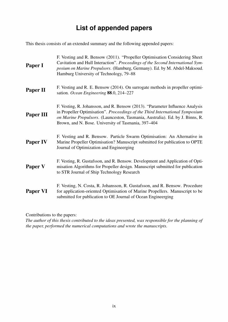
This thesis consists of an extended summary and the following appended papers:

Paper IF. Vesting and R. Bensow (2011). “Propeller Optimisation Considering SheetCavitation and Hull Interaction”. Proceedings of the Second International Sym-posium on Marine Propulsors. (Hamburg, Germany). Ed. by M. Abdel-Maksoud.Hamburg University of Technology, 79–88

Paper II F. Vesting and R. E. Bensow (2014). On surrogate methods in propeller optimi-sation. Ocean Engineering 88.0, 214–227

Paper IIIF. Vesting, R. Johansson, and R. Bensow (2013). “Parameter Influence Analysisin Propeller Optimisation”. Proceedings of the Third International Symposiumon Marine Propulsors. (Launceston, Tasmania, Australia). Ed. by J. Binns, R.Brown, and N. Bose. University of Tasmania, 397–404

Paper IVF. Vesting and R. Bensow. Particle Swarm Optimisation: An Alternative inMarine Propeller Optimisation? Manuscript submitted for publication to OPTEJournal of Optimization and Engineerging

Paper VF. Vesting, R. Gustafsson, and R. Bensow. Development and Application of Opti-misation Algorithms for Propeller design. Manuscript submitted for publicationto STR Journal of Ship Technology Research

Paper VIF. Vesting, N. Costa, R. Johansson, R. Gustafsson, and R. Bensow. Procedurefor application-oriented Optimisation of Marine Propellers. Manuscript to besubmitted for publication to OE Journal of Ocean Engineerging

Contributions to the papers:The author of this thesis contributed to the ideas presented, was responsible for the planning ofthe paper, performed the numerical computations and wrote the manuscripts.

ix

Nomenclature

AcronymsAS Adaptive Surrogate-assistedBEM Boundary Element MethodCCNN Cascade Correlation Neural NetworkCPP Controllable Pitch PropellerCSR Continuous Service Rating equivalent to NCRCV M Constraint Violation MeasureDNV Det Norske VeritasEASM Explicit Algebraic Stress ModelFAST Fourier Amplitude Sensitivity TestFFNN Feed Forward Neural NetworkFPP Fixed Pitch PropellerIMO International Maritime OrganisationIT TC International Towing Tank ConferenceLES Large Eddy SimulationLpp Length between perpendicularsMARIN Maritime Research Institute NetherlandsMCR Maximum Continuous RatingNCR Maximum Continuous Rating equivalent to CSRRANS Reynolds Averaged Navier-StokesSANA Surrogate Assisted Neighbourhood AssessmentSMCR Specified Maximum Continuous RatingV LM Vortex Lattice Method

Variables and notations(u,v,w) Velocity components in (x,y,z) directions(x,y,z) 3D Cartesian coordinatesη ,ηB Propeller efficiency behind shipηH Hull efficiencyηS Shaft efficiencyΓ Discrete vortexγ(x) Vorticity distribution on 2DΓB Strength of bound vortex on blade surfacesΓW Strength of free shed vortex on wake surfacesn Normal vector to camber surfacev Velocity vectorω Dissipation rateφ Position angle for wake velocityφ Velocity potentialρ Fluid mass densityθ Blade angle

xi

θ0 Angular coordinateAn,Bn Fourier series harmonic coefficientsD Propeller diameterg Acceleration due to gravityh Cavity thicknessJS Advance ratiok Turbulence kinetic energyKQ Propeller torque coefficientKT Thrust coefficientL Liftl Cavity lengthn Harmonic numbern Number of propeller revolutions per secondp Pressurep Propeller induced pressure pulsesPB Brake powerq(x) Cavity source distributionQB Discrete line sources for blade thicknessQC Discrete line sources for cavity thicknessR Propeller radiust TimeU∞ Flow speed at infinityVa,Vr,Vt Time-averaged velocityVS Ship speedwt Total wake fractiony+ Non-dimensional wall distanceZ Number of propeller blades

xii

Any sufficiently advanced technology isindistinguishable from magic.

Arthur C. Clarke

1 Introduction

The marine screw propeller is a fascinating invention. It transmits power into a fluid medium byconverting rotational motion into thrust. Hydrofoils are arranged on a shaft, which are shaped andaligned such that a pressure difference develops between both blade sides, thereby accelerating thefluid. Today’s propeller blade shapes are highly complex free-form surfaces that require carefuldesign considerations and accurate manufacturing engineering.

Inspired by the Archimedes’ screw and Leonardo da Vinci’s principle of a helicopter, the firstconcepts of ship propellers emerged in the 18th century as suggestions to propel ships, e.g., thoseby Robert Hooke, Daniel Bernoulli and James Watt. These earlier fan-like propellers resembletoday’s propellers in appearance. However, the first marine propellers used in applications wereArchimedean screw-type propellers, which powered a submarine developed by David Bushnell.The developments accelerated at the beginning of the 19th century, when the increased power andreliability of steam engines required an improvement in propulsion for sea-going ships. Severalinventors equipped steam-driven ships with different types and constellations of propellers. JosefRessel, for instance, designed an Archimedean screw-type propeller with two blades, each of asingle revolution, and equipped the steam vessel ’Civetta’ with this propeller in 1829. Figure 1.1provides the handwriting of Josef Ressel for his marine propeller.

In 1836, John Ericsson proposed a propulsion system of two contra-rotating propellers basedon the Bernoulli-type propeller. The propellers were mounted behind the rudder, which resulted inhindered manoeuvrability. Francis Pettit Smith tested a wooden Archimedean screw, designedwith two turns, on a 30-foot vessel in 1837. The propeller accidentally broke, and suddenly,with only a single turn left, the achievable ship speed doubled. These inventors, to name onlya few, contributed to the development of the propeller. All of them encountered suspicion andinitial opposition from stakeholders at the time. The fact that propeller design stabilised onlytowards the end of that century highlights that the effectiveness of the propeller was not entirelyunderstood. However, screw propellers were beneficial in multiple fields, compared to typicalpaddle propulsion, and became the dominant propulsion type. Since then, many attempts havebeen made to minimise the amount of input energy to the propeller; however, the general formevolved in the 19th century.

Propellers are still under development, and their appearance today differs from that of propellersfrom two or three decades ago. At present, modifications to the propeller design are widelymotivated by technology developments (e.g., manufacturing technology or material technology),regulations (e.g., DNV SILENT class notation (DNV, 2010)) or costs (e.g., production andoperation costs), which are driven by the general developments of shipping. The globalised

1

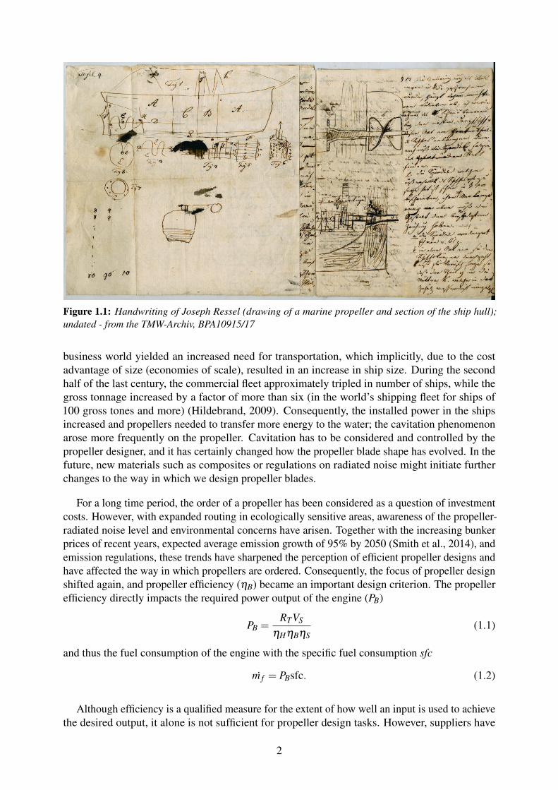
Figure 1.1: Handwriting of Joseph Ressel (drawing of a marine propeller and section of the ship hull);undated - from the TMW-Archiv, BPA10915/17

business world yielded an increased need for transportation, which implicitly, due to the costadvantage of size (economies of scale), resulted in an increase in ship size. During the secondhalf of the last century, the commercial fleet approximately tripled in number of ships, while thegross tonnage increased by a factor of more than six (in the world’s shipping fleet for ships of100 gross tones and more) (Hildebrand, 2009). Consequently, the installed power in the shipsincreased and propellers needed to transfer more energy to the water; the cavitation phenomenonarose more frequently on the propeller. Cavitation has to be considered and controlled by thepropeller designer, and it has certainly changed how the propeller blade shape has evolved. In thefuture, new materials such as composites or regulations on radiated noise might initiate furtherchanges to the way in which we design propeller blades.

For a long time period, the order of a propeller has been considered as a question of investmentcosts. However, with expanded routing in ecologically sensitive areas, awareness of the propeller-radiated noise level and environmental concerns have arisen. Together with the increasing bunkerprices of recent years, expected average emission growth of 95% by 2050 (Smith et al., 2014), andemission regulations, these trends have sharpened the perception of efficient propeller designs andhave affected the way in which propellers are ordered. Consequently, the focus of propeller designshifted again, and propeller efficiency (ηB) became an important design criterion. The propellerefficiency directly impacts the required power output of the engine (PB)

PB =RTVS

ηHηBηS(1.1)

and thus the fuel consumption of the engine with the specific fuel consumption sfc

m f = PBsfc. (1.2)

Although efficiency is a qualified measure for the extent of how well an input is used to achievethe desired output, it alone is not sufficient for propeller design tasks. However, suppliers have

2

experienced a change in the customers’ perspective towards a situation in which only the propellerefficiency and fuel consumption have become the major selection criteria (Grunditz, 2015).

The additional awareness enhances competition. In fact, suppliers more frequently attendcomparative performance competitions, where the ranking is based entirely on the propeller effi-ciency and estimated fuel consumption. In such competitions, the fuel consumption is commonlyverified in impartial test facilities, where model tests are conducted with a self-propelled modeland the results are converted to full scale according to the standard ITTC method (ITTC, 1999).This competition and evaluation practice is generally improving the propeller design, yet it hasinitiated a worrying trend of suboptimal designs with high-efficiency performance, disregardingother performance characteristics, e.g., risk for erosion, propeller-induced vibration and variableoperating conditions (Grunditz, 2015).

Propeller design is a highly complex procedure, involving many influencing factors. Tuningthe propeller geometry towards efficiency also changes its characteristics with regard to vibration,inboard noise and cavitation behaviour, which will most likely occur when the propeller is inoperation. The propeller experiences varying inflow conditions while travelling through thecircumferential wake. This causes a varying load on the propeller blade during one revolutionand results in a local pressure drop around the blade. Depending on the operating conditions,e.g., submergence of the propeller shaft or rotational speed, the pressure sags below the vapourpressure and cavitation, i.e., vapour pockets in the liquid, can be observed at the propeller. Whenagain entering high-pressure regions, the cavities collapse extremely rapidly and may cause noiseand vibration, which are transferred to the ship’s hull, and cause erosion on the propeller or therudder. Cavitation and propeller-induced pressure pulses are the most evident propeller effectscontradictory to efficiency. Consequently, the only solution is to find a trade-off blade geometrythat is adapted to the flow and therefore only valid for a certain ship and the specific operatingconditions. To satisfy the ship owner’s expectations and to deliver a practical design, the designerhas to not only consider and control the cavitation but also constrain static and dynamic bladestresses, classification requirements and, in the case of controllable pitch propellers, hub strengthand blade clearance.

Thus, propeller design is truly an art of trading performances and requirements, which isnaturally a multi-objective and multi-disciplinary procedure and which can only be accomplishedin an iterative manner. Common practice is to develop a preliminary design concept and improvethis by subsequently evaluating all applied objectives and constraints to find the best compromise.The various requirements together with seemingly countless modifications to such a free-formsurface lead to a large number of alternatives to be studied and thus place restrictions on thenumerical analysis tools. The blade geometry is, during the design synthesis, evolved by thedesigner’s experience towards the design philosophy and considered as the optimal design. Withsufficient time, a designer can efficiently analyse the design space and reach, driven by theknowledge, the best possible design. In such a procedure, time is the most limiting restriction.

The length of time available for a product being conceived until it is ready for sale is oneof the most important factors in a world that is changing rapidly at an accelerating pace. Thisholds for most of the engineering design tasks and in particular for the propeller design becauseeach is a unique layout for a certain ship. To be ahead of competitors, a propeller designer needsto present a better design for a specific purpose in a shorter time and at lower costs than theadversary. The current challenge for propeller designers is to develop a propeller that fulfils allrequirements and expectations within the short time length available in the competition races.

3

Thus, although the evaluation of propeller performance requires highly unsteady and physicallyprofoundly complex simulations, it is common practice to apply less accurate but faster potentialmethods (e.g., Mishima, 1996; Griffin et al., 1998; Han et al., 2006; Gaggero et al., 2009; Leeet al., 2010; Bertetta et al., 2012). In an early design stage, potential methods are indispensableand are, in a later design stage, commonly accompanied by either experiments of model propellersor high-fidelity numerical simulations, or both, to validate the performance prediction.

1.1 Background

There have been several different approaches to improve propeller design within the past threedecades. Burnside et al. (1979) presented, for instance, one of the first propeller design recommen-dations with special considerations regarding propeller-induced vibrations. Both analytical andexperimental techniques were considered and indicated that cavitation has a significant influenceon the hull pressure.

More recently, (Mishima, 1996) presented the optimisation of propeller blade geometry withrespect to sheet cavitation, which was predicted using a vortex lattice method (VLM). Mishima(1996) minimised the torque in a single-objective approach, where the objective function wasapproximated first by a linear and finally by a quadratic function. The function coefficients weredetermined using a numerical propeller analysis program. Hence, the actual optimisation wasaccomplished by employing a classical optimisation method of linear and quadratic programming.

Griffin et al. (1998) further developed the non-linear optimisation method and included aquadratic skew distribution. The propeller performance was again analysed using a VLM withcavitation prediction. Griffin et al. (1998) applied constraints on the minimum blade pressuredistribution and thereby prevented the onset of bubble cavitation. The optimisation yielded, withfurther applied constraints on the cavity area and maximal cavity volume, an improved propellerdesign.

Automated propeller optimisation has emerged more frequently in recent years for accom-plishing a large number of design alternatives and thereby supporting the designer during thedesign synthesis and reducing design lead time. Foeth (2015) presented a propeller geometryparametrisation based on database records and the multi-objective optimisation in the behindcondition, applying the derived parameters. Thus, the optimisation was performed with fullinteraction between the propeller changes and hull changes. However, this was computationallyintensive, and no constraints were considered. It is hypothesised that a preliminary optimisation isperformed to determine the main parameter ranges. Berger et al. (2014) presented such an idea in atwo- stage optimisation with propeller hull interaction applied in the second stage, after evaluationof a multi-objective optimisation in a given wake condition. This is an efficient intermediate stepfor assisting the designer in finding the optimal design for a given hull geometry. However, in thepresented approach, only a constraint on thrust equality was applied, and the objective functionwas related to the applied weight factor.

Constrained propeller optimisation was, e.g., presented by Han et al. (2006) with a weightedmulti-objective propeller blade optimisation in a given wake and with constraints on sheet cavita-tion. The results align with Griffin et al. (1998), showing considerable improvements in cavitationperformance when applying cavity volume and area constraints.

Similarly, Kamarlouei et al. (2014) applied an optimisation in a fixed wake, with cavitation

4

constraints on the blade loading (Keller criteria) and the Bucket criteria. In contrast to Hanet al. (2006), Kamarlouei et al. (2014) also included constraints for the blade strength, althoughwith simplification to cantilever beam theory. Bertetta et al. (2012) presented the multi-objectiveoptimisation of a controllable pitch propeller (CPP), with the main aim of reducing the facecavitation and thereby the resulting radiated noise. The common dominator of the aforementionedexamples is the applied numerical evaluation of the propeller performance, which is based onpotential methods. However, the applied cavitation constraints are based on general characteristics,e.g., the maximum cavitation volume or the cavity areas, and constraints on blade strength wereonly included by Kamarlouei et al. (2014).

1.2 Motivation

The recent work outlined above highlights the growing interest in designing the optimal propellershape. However, in practice, evaluations of numerous limitations and parameters require variousjudgements by experienced propeller designers to make decisions during the development, wherelead time is the most limiting factor during the investigation of design alternatives. With theenhanced accuracy of numerical tools and increasing computational power, particularly in desktopworkstations, this task can be facilitated by automated optimisation. The challenge is to developalgorithms that not only create variants automatically but that also handle constraints and makedecisions in favour of the designer’s decision to find the global optimum.

The purpose of this thesis is to further improve the state-of-the-art of the propeller designprocedure by supplementing the propeller designer with automated optimisation. The overarchingresearch question is therefore the following:

How can optimisation be adapted to propeller design on an everyday use basis to efficiently assistthe designer using automated optimisation and simultaneously enhance the multi-disciplinaryevaluation of the manual design procedure to reduce the lead time in product development?

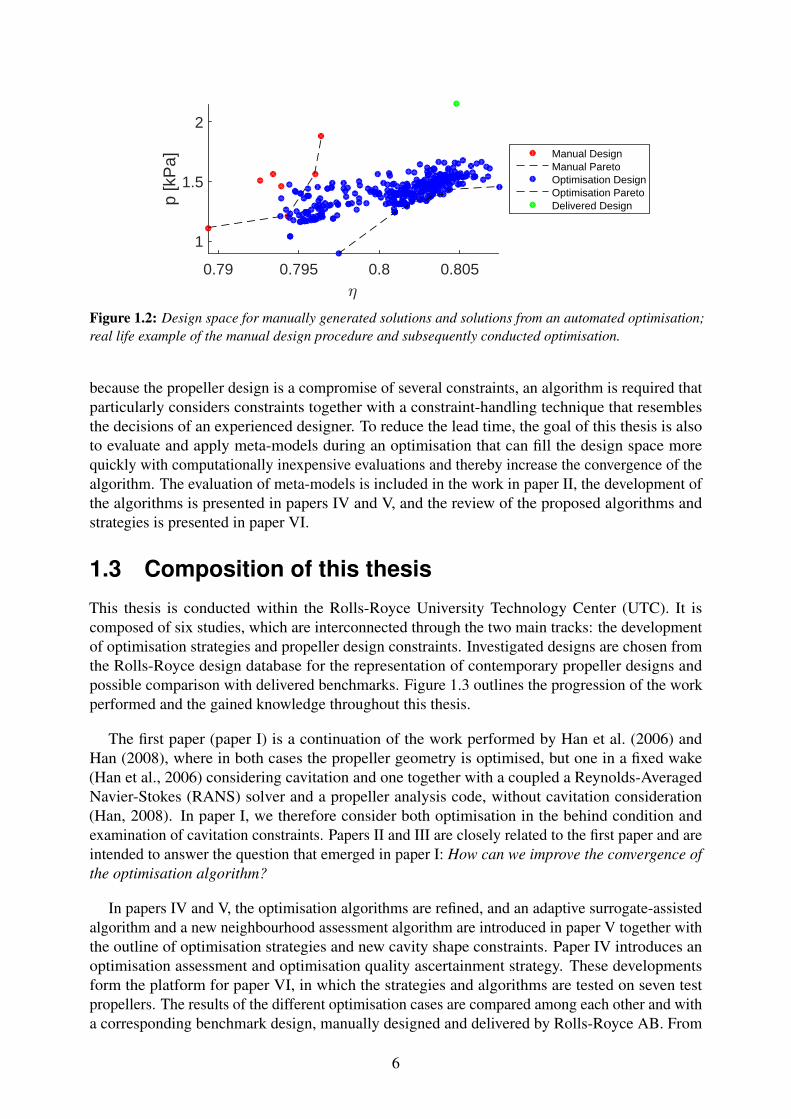
This thesis therefore examines two tracks: i) the development of strategies and concepts forpropeller optimisation, with the objective of developing optimisation algorithms that enhanceconvergence and consideration of constraints, and ii) the extension and exploration of constraintsthat are adapted to the principles and design considerations of the manual design procedure. Theart of designing a propeller, with the multi-disciplinary evaluation and consideration of numerouslimitations, limits a systematic investigation of the design space, which is due to the availabletime generally being limited. With automated optimisation, we can fill the design space withnumerous designs, which gravitate, guided by the optimisation algorithm, towards an optimaldesign. Figure 1.2 exemplifies the distribution of variants on objective space through the manualapproach ( ), where the designer creates several (typically 10-30) designs and determines themost suitable among these. However, with automatically generated designs ( ) that incorporatethe design constraints and strategies, the design space can readily be filled to find better designalternatives faster.

An automated propeller optimisation procedure requires a judgement of a design variant withoutinteraction of the designer. The objective of this thesis is thus to develop constraints that condenseinformation of the design into single values while enabling connection to geometry changes tothe critical design characteristics. To achieve this objective, this thesis focuses in particular onconstraints in cavitation that adapt to the shape of the cavity. The work on cavitation constraintsis initiated in paper I and is continuously developed further and finalised in paper V. However,

5

2

0.79 0.795 0.8 0.805

p [k

Pa]

1

1.5

2

Manual DesignManual ParetoOptimisation DesignOptimisation ParetoDelivered Design

Figure 1.2: Design space for manually generated solutions and solutions from an automated optimisation;real life example of the manual design procedure and subsequently conducted optimisation.

because the propeller design is a compromise of several constraints, an algorithm is required thatparticularly considers constraints together with a constraint-handling technique that resemblesthe decisions of an experienced designer. To reduce the lead time, the goal of this thesis is alsoto evaluate and apply meta-models during an optimisation that can fill the design space morequickly with computationally inexpensive evaluations and thereby increase the convergence of thealgorithm. The evaluation of meta-models is included in the work in paper II, the development ofthe algorithms is presented in papers IV and V, and the review of the proposed algorithms andstrategies is presented in paper VI.

1.3 Composition of this thesis

This thesis is conducted within the Rolls-Royce University Technology Center (UTC). It iscomposed of six studies, which are interconnected through the two main tracks: the developmentof optimisation strategies and propeller design constraints. Investigated designs are chosen fromthe Rolls-Royce design database for the representation of contemporary propeller designs andpossible comparison with delivered benchmarks. Figure 1.3 outlines the progression of the workperformed and the gained knowledge throughout this thesis.

The first paper (paper I) is a continuation of the work performed by Han et al. (2006) andHan (2008), where in both cases the propeller geometry is optimised, but one in a fixed wake(Han et al., 2006) considering cavitation and one together with a coupled a Reynolds-AveragedNavier-Stokes (RANS) solver and a propeller analysis code, without cavitation consideration(Han, 2008). In paper I, we therefore consider both optimisation in the behind condition andexamination of cavitation constraints. Papers II and III are closely related to the first paper and areintended to answer the question that emerged in paper I: How can we improve the convergence ofthe optimisation algorithm?

In papers IV and V, the optimisation algorithms are refined, and an adaptive surrogate-assistedalgorithm and a new neighbourhood assessment algorithm are introduced in paper V together withthe outline of optimisation strategies and new cavity shape constraints. Paper IV introduces anoptimisation assessment and optimisation quality ascertainment strategy. These developmentsform the platform for paper VI, in which the strategies and algorithms are tested on seven testpropellers. The results of the different optimisation cases are compared among each other and witha corresponding benchmark design, manually designed and delivered by Rolls-Royce AB. From

6

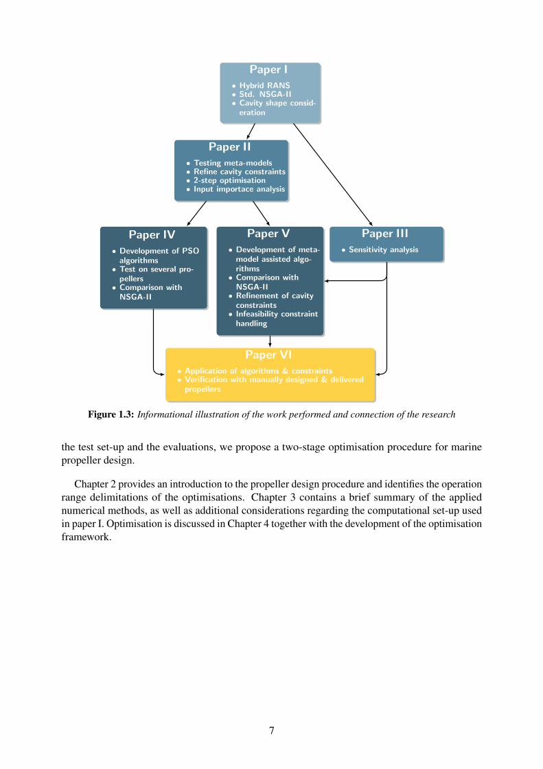
Paper I• Hybrid RANS• Std. NSGA-II• Cavity shape consid-

eration

Paper II• Testing meta-models• Refine cavity constraints• 2-step optimisation• Input importace analysis

Paper III• Sensitivity analysis

Paper IV• Development of PSO

algorithms• Test on several pro-

pellers• Comparison with

NSGA-II

Paper V• Development of meta-

model assisted algo-rithms• Comparison with

NSGA-II• Refinement of cavity

constraints• Infeasibility constraint

handling

Paper VI• Application of algorithms & constraints• Verification with manually designed & delivered

propellers

Figure 1.3: Informational illustration of the work performed and connection of the research

the test set-up and the evaluations, we propose a two-stage optimisation procedure for marinepropeller design.

Chapter 2 provides an introduction to the propeller design procedure and identifies the operationrange delimitations of the optimisations. Chapter 3 contains a brief summary of the appliednumerical methods, as well as additional considerations regarding the computational set-up usedin paper I. Optimisation is discussed in Chapter 4 together with the development of the optimisationframework.

7

The computer is incredibly fast, accurate,and stupid. Man is unbelievably slow,inaccurate, and brilliant. The marriage ofthe two is a force beyond calculation.

Leo Cherne

2 Propeller Design

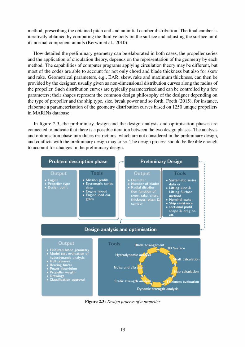
Propeller design is the art of synthesising multi-disciplinary requirements and limitations intoa cohesive final product that efficiently meets the features of a specific ship. It is an iterativeprocedure that can generally be divided into three interacting phases: i) the problem description,ii) the preliminary design and iii) the design analysis and optimisation phases. A flowchart of thepropeller design phases is presented in figure 2.3, which provides an overview of the three phasesand includes both tools that the designer uses and the expected outcome of each phase. In commonengineering design problems, there is a fourth phases in which the design is evaluated, commonlywith a prototype. However, this is rarely possible in propeller design due to the uniqueness ofthe designed propeller and because the evaluation occurs using full-scale sea trial tests with thefinal product. Therefore, propeller design requires particular attention in the design analysis andoptimisation phase. Automated optimisation approaches can support the designer in finding betterdesigns faster.

2.1 Problem description

The primary task in the problem definition phase is the determination and correct selection of thedesign point for the propeller. However, this requires the determination of the propeller type andthe selection of an engine. Hence, the problem description phase typically starts with an evaluationof the vessel: What is the ship’s purpose? Where will it operate? What is the hull maintenanceprocedure? Various operating conditions that the ship experiences during its lifetime are usuallysummarised in a mission profile of the ship, which is provided by the ship’s owner. It determinesthe portion of time that a ship travels at a certain speed and thus outlines the economical designpoint. However, the propeller also has to match the engine characteristics for a good performance.The wrong selection of the design point results in suboptimal operation of the engine at otheroperating conditions. This is particularly important for a fixed pitch propeller (FPP) becausethe design is only valid for one condition, but even the sectional profiles of controllable pitchpropellers (CPP) are optimised for only one inflow condition.

The ship’s requirements also determine the propulsor or rather the propeller type. Systematicseries data, e.g., by Van Manen (1966), Blount (1993) or Tachmindji et al. (1957), assist the de-signer in selecting a suitable propeller type. However, initial costs, running costs and maintenancecosts also determine the type of propeller. Once the propeller type and the engine are selected,the propeller demand and engine power supply need to be matched, considering that the ship

9

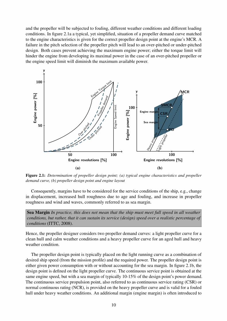
and the propeller will be subjected to fouling, different weather conditions and different loadingconditions. In figure 2.1a a typical, yet simplified, situation of a propeller demand curve matchedto the engine characteristics is given for the correct propeller design point at the engine’s MCR. Afailure in the pitch selection of the propeller pitch will lead to an over-pitched or under-pitcheddesign. Both cases prevent achieving the maximum engine power; either the torque limit willhinder the engine from developing its maximal power in the case of an over-pitched propeller orthe engine speed limit will diminish the maximum available power.

y

Engine revolutions [%]

Enginepower

[%]

50 100

50

100

Engine T

orque limit

EngineSpe edlim

it

Propellerdemand

Overpitched

Under p

itched

(a)

y


Enginepower

[%]

100

100

Heavy

propeller

Lightpropeller

Engine margin

Sea margin

PD

CSR

SMCR

MCR

(b)

Figure 2.1: Determination of propeller design point; (a) typical engine characteristics and propellerdemand curve, (b) propeller design point and engine layout

Consequently, margins have to be considered for the service conditions of the ship, e.g., changein displacement, increased hull roughness due to age and fouling, and increase in propellerroughness and wind and waves, commonly referred to as sea margin.

Sea Margin In practice, this does not mean that the ship must meet full speed in all weatherconditions, but rather, that it can sustain its service (design) speed over a realistic percentage ofconditions (ITTC, 2008).

Hence, the propeller designer considers two propeller demand curves: a light propeller curve for aclean hull and calm weather conditions and a heavy propeller curve for an aged hull and heavyweather condition.

The propeller design point is typically placed on the light running curve as a combination ofdesired ship speed (from the mission profile) and the required power. The propeller design point iseither given power consumption with or without accounting for the sea margin. In figure 2.1b, thedesign point is defined on the light propeller curve. The continuous service point is obtained at thesame engine speed, but with a sea margin of typically 10-15% of the design point’s power demand.The continuous service propulsion point, also referred to as continuous service rating (CSR) ornormal continuous rating (NCR), is provided on the heavy propeller curve and is valid for a fouledhull under heavy weather conditions. An additional margin (engine margin) is often introduced to

10

reduce maintenance costs in keeping the machine away from peak performance over the lifetime.

Engine Margin The engine operation margin describes the mechanical and the thermodynamicpower reserve for the economical operation of the engine(s) with respect to reasonably low fueland maintenance costs (ITTC, 2008).

The final margin yields the specified MCR (SMCR), which is the maximum rating requiredfor continuous operation of the engine. The SMCR may be different from the engine nominalmaximum continuous rating (MCR), which is the engine’s limit for continuous operation (nominalMCR in figure 2.1b).

The shaded area in figure 2.1b presents the engine layout diagram, limited by two constantengine speed lines and two constant mean effective pressure lines. Within the outlined area, theSMCR point can be defined to meet the optimum operation profile for the ship, where the lowestfuel consumption will be achieved at 70 to 80% power of SMCR for both electronically andmechanically controlled engines (MAN, 2011).

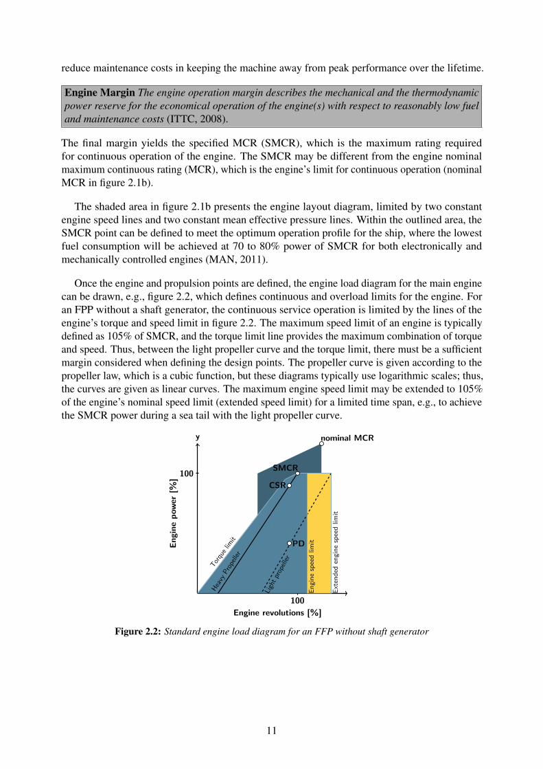
Once the engine and propulsion points are defined, the engine load diagram for the main enginecan be drawn, e.g., figure 2.2, which defines continuous and overload limits for the engine. Foran FPP without a shaft generator, the continuous service operation is limited by the lines of theengine’s torque and speed limit in figure 2.2. The maximum speed limit of an engine is typicallydefined as 105% of SMCR, and the torque limit line provides the maximum combination of torqueand speed. Thus, between the light propeller curve and the torque limit, there must be a sufficientmargin considered when defining the design points. The propeller curve is given according to thepropeller law, which is a cubic function, but these diagrams typically use logarithmic scales; thus,the curves are given as linear curves. The maximum engine speed limit may be extended to 105%of the engine’s nominal speed limit (extended speed limit) for a limited time span, e.g., to achievethe SMCR power during a sea tail with the light propeller curve.

y


Enginepower

[%]

100

100

Heavy

Propeller

Lightpropeller

Extended

enginespe edli m

it

Eng inespe edlim

it

Torquelim

it PD

CSR

SMCR

nominal MCR

Figure 2.2: Standard engine load diagram for an FFP without shaft generator

11

2.2 Preliminary design

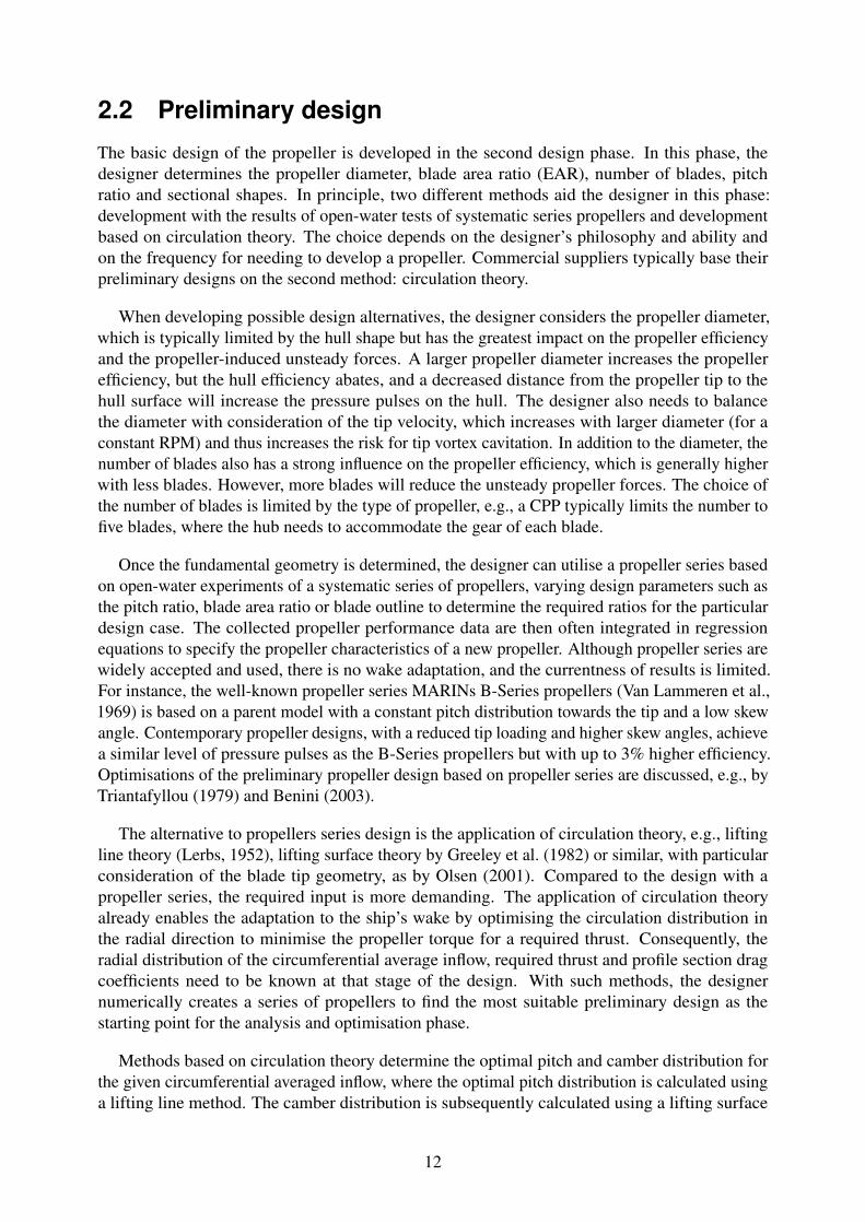
The basic design of the propeller is developed in the second design phase. In this phase, thedesigner determines the propeller diameter, blade area ratio (EAR), number of blades, pitchratio and sectional shapes. In principle, two different methods aid the designer in this phase:development with the results of open-water tests of systematic series propellers and developmentbased on circulation theory. The choice depends on the designer’s philosophy and ability andon the frequency for needing to develop a propeller. Commercial suppliers typically base theirpreliminary designs on the second method: circulation theory.

When developing possible design alternatives, the designer considers the propeller diameter,which is typically limited by the hull shape but has the greatest impact on the propeller efficiencyand the propeller-induced unsteady forces. A larger propeller diameter increases the propellerefficiency, but the hull efficiency abates, and a decreased distance from the propeller tip to thehull surface will increase the pressure pulses on the hull. The designer also needs to balancethe diameter with consideration of the tip velocity, which increases with larger diameter (for aconstant RPM) and thus increases the risk for tip vortex cavitation. In addition to the diameter, thenumber of blades also has a strong influence on the propeller efficiency, which is generally higherwith less blades. However, more blades will reduce the unsteady propeller forces. The choice ofthe number of blades is limited by the type of propeller, e.g., a CPP typically limits the number tofive blades, where the hub needs to accommodate the gear of each blade.

Once the fundamental geometry is determined, the designer can utilise a propeller series basedon open-water experiments of a systematic series of propellers, varying design parameters such asthe pitch ratio, blade area ratio or blade outline to determine the required ratios for the particulardesign case. The collected propeller performance data are then often integrated in regressionequations to specify the propeller characteristics of a new propeller. Although propeller series arewidely accepted and used, there is no wake adaptation, and the currentness of results is limited.For instance, the well-known propeller series MARINs B-Series propellers (Van Lammeren et al.,1969) is based on a parent model with a constant pitch distribution towards the tip and a low skewangle. Contemporary propeller designs, with a reduced tip loading and higher skew angles, achievea similar level of pressure pulses as the B-Series propellers but with up to 3% higher efficiency.Optimisations of the preliminary propeller design based on propeller series are discussed, e.g., byTriantafyllou (1979) and Benini (2003).

The alternative to propellers series design is the application of circulation theory, e.g., liftingline theory (Lerbs, 1952), lifting surface theory by Greeley et al. (1982) or similar, with particularconsideration of the blade tip geometry, as by Olsen (2001). Compared to the design with apropeller series, the required input is more demanding. The application of circulation theoryalready enables the adaptation to the ship’s wake by optimising the circulation distribution inthe radial direction to minimise the propeller torque for a required thrust. Consequently, theradial distribution of the circumferential average inflow, required thrust and profile section dragcoefficients need to be known at that stage of the design. With such methods, the designernumerically creates a series of propellers to find the most suitable preliminary design as thestarting point for the analysis and optimisation phase.

Methods based on circulation theory determine the optimal pitch and camber distribution forthe given circumferential averaged inflow, where the optimal pitch distribution is calculated usinga lifting line method. The camber distribution is subsequently calculated using a lifting surface

12

method, prescribing the obtained pitch and and an initial camber distribution. The final camber isiteratively obtained by computing the fluid velocity on the surface and adjusting the surface untilits normal component annuls (Kerwin et al., 2010).

How detailed the preliminary geometry can be elaborated in both cases, the propeller seriesand the application of circulation theory, depends on the representation of the geometry by eachmethod. The capabilities of computer programs applying circulation theory may be different, butmost of the codes are able to account for not only chord and blade thickness but also for skewand rake. Geometrical parameters, e.g., EAR, skew, rake and maximum thickness, can then beprovided by the designer, usually given as non-dimensional distribution curves along the radius ofthe propeller. Such distribution curves are typically parameterised and can be controlled by a fewparameters; their shapes represent the common design philosophy of the designer depending onthe type of propeller and the ship type, size, break power and so forth. Foeth (2015), for instance,elaborate a parameterisation of the geometry distribution curves based on 1250 unique propellersin MARINs database.

In figure 2.3, the preliminary design and the design analysis and optimisation phases areconnected to indicate that there is a possible iteration between the two design phases. The analysisand optimisation phase introduces restrictions, which are not considered in the preliminary design,and conflicts with the preliminary design may arise. The design process should be flexible enoughto account for changes in the preliminary design.

Problem description phase

Output• Engine• Propeller type• Design point

Tools• Mission profile• Systematic series

data• Engine layout• Engine load dia-

gram

Preliminary Design

Output• Diameter• Number of blades• Radial distribu-

tion function ofskew, rake, chord,thickness, pitch &camber

Tools• Systematic series

data or• Lifting Line &

Lifting Surfacemethod• Nominal wake• Ship resistance• sectional profil

shape & drag co-eff.

Design analysis and optimisation

Blade arrangement

Noise and vibration

Static strength analysis

Hydrodynamic analysis

Dynamic strength analysis

Thickness evaluation

Hub calculation

Shaft calculation

3D SurfaceToolsOutput

• Finalized blade geometry• Model test evaluation of

hydordynamic analysis• Hull pressure• Bearing forces• Power absorbtion• Propeller weigth• Drawings• Classification approval

Figure 2.3: Design process of a propeller

13

2.3 Design analysis and optimisation

The preliminary design is elaborated in the design analysis and optimisation phase with numericalmethods and experiments, respectively, to develop the detailed geometry. In this phase, the designis optimised with detailed changes of the blade geometry to find the best compromise. Unlike thepreliminary design phase, where the blade geometry is only partly specified and partly designedusing the numerical methods as an optimisation of circulation distribution, in the analysis phase,the entire geometry is known and the performance of the propeller is analysed using numericalmethods. This analysis requires detailed inflow information, obtained either by simulation ofthe ship together with the propeller or by calculation of effective inflow velocities, for detailedestimation of the propeller forces and cavitation.

The design analysis and optimisation phase can also be accomplished by systematic series andempirical formulation. The application of numerical methods and model tests again depend on thecapabilities of the designer and the requirements of the customer. For small vessels where onlylittle information of the flow around the hull is known, the design procedure based on a series ofpropellers and an adaptation based on cavitation criteria, e.g. Keller criteria, propeller strengthevaluation by cantilever beam theory followed by a fatigue estimate and blade thickness accordingto classification rules, may be sufficient. However, for larger vessels, propeller suppliers typicallyutilise numerical methods of variable fidelity and experiments of model propellers to evaluate thesimulations.

The final part of the design phase finalises the design such that the propeller is ready formanufacturing. In addition to a detailed geometry representation, this also requires constraintsthat restrict the design and yield designs that are manufacturable and that conform with theclassification rules. Hence, this phase is about manipulating the geometry iteratively to find thebest compromise that is feasible and that provides the best performance. It is a design spiral thatincludes multi-disciplinary constraints and objectives and that is traversed by the designer severaltimes. The process is presented as a continuous circle (figure 2.3); however, the cycle may beinterrupted when the performance is not acceptable and design changes are required.

Typical constraints are cavitation, static and dynamic blade stresses and classification regula-tions that are often contradictory to the typical objectives (propeller efficiency, propeller-inducedpressure pulse and blade weight). However, when the detailed geometry is already developedas a 3-dimensional surface, constraints apply on the arrangement of the blade on the hub, bladecollision and details of the blade edges. The designer analyses the hydrodynamic performance toobtain the propeller forces and thus the power consumption and evaluates cavitation on the blade,which typically has to be constrained to reduce the risk for erosion. Propeller-induced vibrationand noise are related to the hydrodynamic performance but often require specific calculations.Static strength and possibly ice loads acting on the propeller blades are, with contemporary bladeshapes, calculated using finite element methods (FEM). The obtained maximum stress level issubsequently applied in a dynamic strength analysis to ensure the service life of the propeller.Classification approval requires not only providing a minimum blade thickness but also calcu-lations of the hub and the shaft, e.g., blade bearing forces, blade bolt diameter or required oilpressure to pitch the blade in the case of a CPP.

The outlined iterative procedure requires an experienced propeller designer to systematicallymodify the geometry locally to accommodate all the requirements on the design. It can be comevery time consuming to account for all multi-disciplinary evaluations. Therefore, an automated

14

optimisation can assist the designer in accomplishing this task faster and with a better quality ofthe final design.

2.4 Design evaluation

After the optimal propeller design is obtained, all limitations and demands are satisfied, and thedesign is approved, the propeller will be manufactured. The evaluation of the design is generallyaccomplished during full-scale speed and powering trials with the final product, which are typicallyconducted at the end of the ship-building phase with a new, light and clean hull. The problem of seatrials is to correct the measured data to ideal, typically contracted, conditions, which is addressedby ITTC (2002). It may also be required to evaluate the ship and propeller performance in serviceconditions to reduce operating costs and to collect data for possible sister ships (Andersen et al.,2005). Mismatching the specified design criteria results in costly modifications of the propeller.

15

The purpose of computing is insight, notnumbers

Richard Hamming

3 Numerical Methods

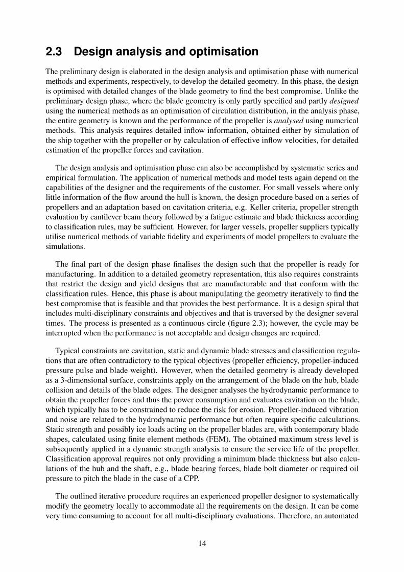
There is a broad range of numerical simulation methodologies and tools that can be consulted fordesigning a marine propeller. Simulations for propeller design might begin with predicting the barehull resistance and might continue, with increasing complexity, with self-propelled simulations,cavitation simulations and pressure pulse computation. One might end with ship simulationsin waves or simulations of manoeuvrability. Each of these applications can be conducted atdifferent levels of computational fidelity and with a variable approximation level; an exampleof method fidelity for propeller simulations is given in 3.1. Each method embodies differentlevels of neglected physical effects. The numerical methods applied in this thesis are limited tothe highlighted methods (hybrid RANS, lifting surface and lifting line methods). Hybrid RANSsimulations are found to be on the edge of being practical in optimisation tasks. In particular, dueto the unsteady nature of the rotating propeller, transient simulations are required and simulationsmight take several weeks, which is too demanding for automated optimisation.

Resource efficiency

Tim

e

Reality Neglected physical effects

Experiment

LES

Fully unsteady RANS

Hybrid RANS

BEMLifting surface method

Lifting line method

Time ’limit’ for practical optimisation

Figure 3.1: Variable fidelity of numerical methods for propeller simulation

3.1 Potential flow propeller analysis model

The prediction of propeller performance using potential methods requires several assumptions,which are applied to simplify the complex flow. The operational domain for a marine propeller is

17

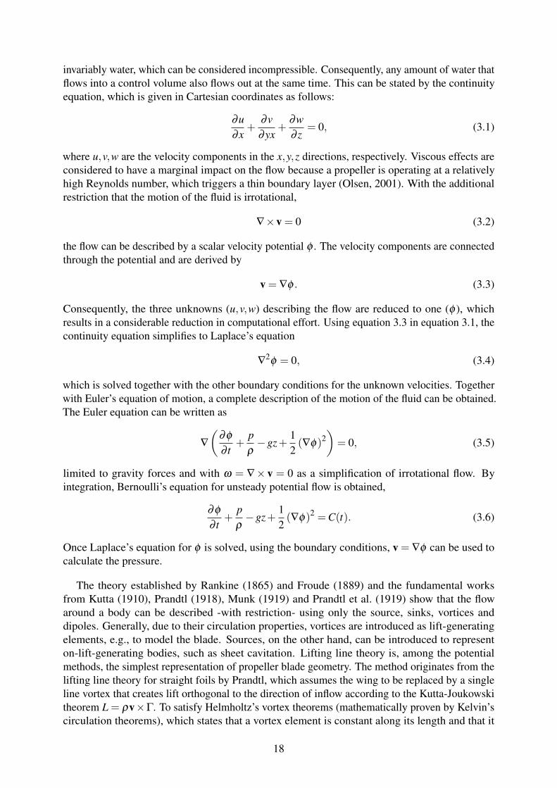
invariably water, which can be considered incompressible. Consequently, any amount of water thatflows into a control volume also flows out at the same time. This can be stated by the continuityequation, which is given in Cartesian coordinates as follows:

∂u∂x

+∂v∂yx

+∂w∂ z

= 0, (3.1)

where u,v,w are the velocity components in the x,y,z directions, respectively. Viscous effects areconsidered to have a marginal impact on the flow because a propeller is operating at a relativelyhigh Reynolds number, which triggers a thin boundary layer (Olsen, 2001). With the additionalrestriction that the motion of the fluid is irrotational,

∇×v = 0 (3.2)

the flow can be described by a scalar velocity potential φ . The velocity components are connectedthrough the potential and are derived by

v = ∇φ . (3.3)

Consequently, the three unknowns (u,v,w) describing the flow are reduced to one (φ ), whichresults in a considerable reduction in computational effort. Using equation 3.3 in equation 3.1, thecontinuity equation simplifies to Laplace’s equation

∇2φ = 0, (3.4)

which is solved together with the other boundary conditions for the unknown velocities. Togetherwith Euler’s equation of motion, a complete description of the motion of the fluid can be obtained.The Euler equation can be written as

∇(

∂φ∂ t

+pρ−gz+

12(∇φ)2

)= 0, (3.5)

limited to gravity forces and with ω = ∇× v = 0 as a simplification of irrotational flow. Byintegration, Bernoulli’s equation for unsteady potential flow is obtained,

∂φ∂ t

+pρ−gz+

12(∇φ)2 =C(t). (3.6)

Once Laplace’s equation for φ is solved, using the boundary conditions, v = ∇φ can be used tocalculate the pressure.

The theory established by Rankine (1865) and Froude (1889) and the fundamental worksfrom Kutta (1910), Prandtl (1918), Munk (1919) and Prandtl et al. (1919) show that the flowaround a body can be described -with restriction- using only the source, sinks, vortices anddipoles. Generally, due to their circulation properties, vortices are introduced as lift-generatingelements, e.g., to model the blade. Sources, on the other hand, can be introduced to representon-lift-generating bodies, such as sheet cavitation. Lifting line theory is, among the potentialmethods, the simplest representation of propeller blade geometry. The method originates from thelifting line theory for straight foils by Prandtl, which assumes the wing to be replaced by a singleline vortex that creates lift orthogonal to the direction of inflow according to the Kutta-Joukowskitheorem L = ρv×Γ. To satisfy Helmholtz’s vortex theorems (mathematically proven by Kelvin’scirculation theorems), which states that a vortex element is constant along its length and that it

18

cannot end in the interior of the fluid, non-lift-generating vortices are introduced at both ends ofthe wing. They form together with the bound vortex the so-called horseshoe vortex and continuedownstream. By introducing several bound vortices that vary in strength from section to sectionand corresponding free vorticity, the wing representation becomes more realistic. The methodis adapted to the marine propeller problem in Lerbs analysis method for a moderately loadedpropeller (Lerbs, 1952) and is a vital part of the propeller design procedures to either the optimalcirculation distribution or the blade geometry corresponding to a given radial load distribution(Bertram, 2012).

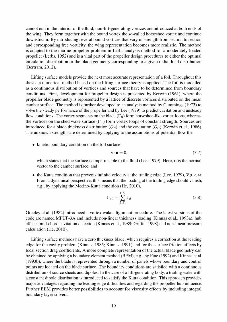
Lifting surface models provide the next most accurate representation of a foil. Throughout thisthesis, a numerical method based on the lifting surface theory is applied. The foil is modelledas a continuous distribution of vortices and sources that have to be determined from boundaryconditions. First, development for propeller design is presented by Kerwin (1961), where thepropeller blade geometry is represented by a lattice of discrete vortices distributed on the meancamber surface. The method is further developed to an analysis method by Cummings (1973) tosolve the steady performance of the propeller and by Lee (1979) to predict cavitation and unsteadyflow conditions. The vortex segments on the blade (ΓB) form horseshoe-like vortex loops, whereasthe vortices on the shed wake surface (Γw) form vortex loops of constant strength. Sources areintroduced for a blade thickness distribution (QB) and the cavitation (QC) (Kerwin et al., 1986).The unknown strengths are determined by applying to the assumptions of potential flow the

• kinetic boundary condition on the foil surface

v ·n = 0, (3.7)

which states that the surface is impermeable to the fluid (Lee, 1979). Here, n is the normalvector to the camber surface, and

• the Kutta condition that prevents infinite velocity at the trailing edge (Lee, 1979), ∇φ < ∞.From a dynamical perspective, this means that the loading at the trailing edge should vanish,e.g., by applying the Morino-Kutta condition (He, 2010),

Γw1 =T.E.

∑L.E.

ΓB (3.8)

Greeley et al. (1982) introduced a vortex wake alignment procedure. The latest versions of thecode are named MPUF-3A and include non-linear thickness loading (Kinnas et al., 1993a), hubeffects, mid-chord cavitation detection (Kinnas et al., 1989; Griffin, 1998) and non-linear pressurecalculation (He, 2010).

Lifting surface methods have a zero thickness blade, which requires a correction at the leadingedge for the cavity problem (Kinnas, 1985; Kinnas, 1991) and for the surface friction effects bylocal section drag coefficients. A more complete representation of the actual blade geometry canbe obtained by applying a boundary element method (BEM), e.g., by Fine (1992) and Kinnas et al.(1993b), where the blade is represented through a number of panels whose boundary and controlpoints are located on the blade surface. The boundary conditions are satisfied with a continuousdistribution of source sheets and dipoles. In the case of a lift-generating body, a trailing wake witha constant dipole distribution is introduced to satisfy the Kutta condition. This approach providesmajor advantages regarding the leading edge difficulties and regarding the propeller hub influence.Further BEM provides better possibilities to account for viscosity effects by including integralboundary layer solvers.

19

3.2 Prediction of propeller cavitation

Turning to the numerical prediction of cavitation, the applied analysis tool MPUF-3A (He et al.,2010, and He et al., 2011) is based on lifting surface theory and in particular on a vortex latticemethod, as described above. The cavity determination follows an iterative process, described byKerwin et al. (1986), and will be outlined in this context briefly.

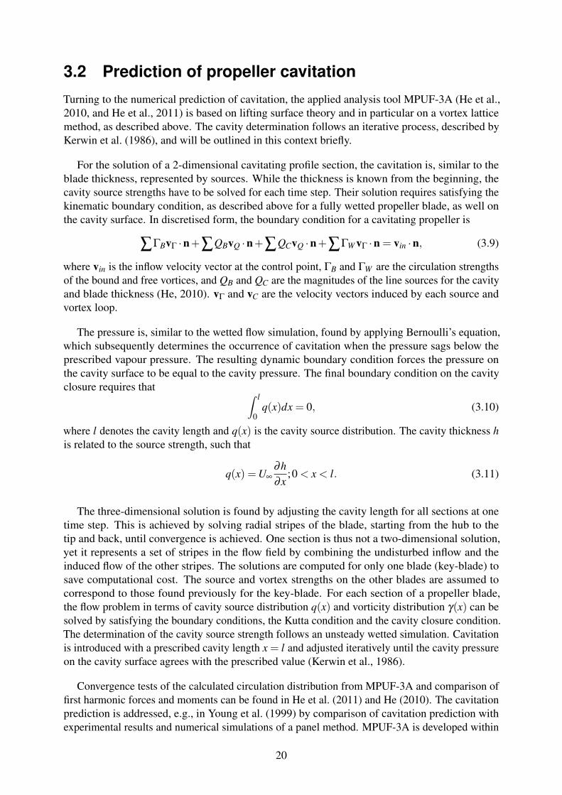
For the solution of a 2-dimensional cavitating profile section, the cavitation is, similar to theblade thickness, represented by sources. While the thickness is known from the beginning, thecavity source strengths have to be solved for each time step. Their solution requires satisfying thekinematic boundary condition, as described above for a fully wetted propeller blade, as well onthe cavity surface. In discretised form, the boundary condition for a cavitating propeller is

∑ΓBvΓ ·n+∑QBvQ ·n+∑QCvQ ·n+∑ΓW vΓ ·n = vin ·n, (3.9)

where vin is the inflow velocity vector at the control point, ΓB and ΓW are the circulation strengthsof the bound and free vortices, and QB and QC are the magnitudes of the line sources for the cavityand blade thickness (He, 2010). vΓ and vC are the velocity vectors induced by each source andvortex loop.

The pressure is, similar to the wetted flow simulation, found by applying Bernoulli’s equation,which subsequently determines the occurrence of cavitation when the pressure sags below theprescribed vapour pressure. The resulting dynamic boundary condition forces the pressure onthe cavity surface to be equal to the cavity pressure. The final boundary condition on the cavityclosure requires that ∫ l

0q(x)dx = 0, (3.10)

where l denotes the cavity length and q(x) is the cavity source distribution. The cavity thickness his related to the source strength, such that

q(x) =U∞∂h∂x

;0 < x < l. (3.11)

The three-dimensional solution is found by adjusting the cavity length for all sections at onetime step. This is achieved by solving radial stripes of the blade, starting from the hub to thetip and back, until convergence is achieved. One section is thus not a two-dimensional solution,yet it represents a set of stripes in the flow field by combining the undisturbed inflow and theinduced flow of the other stripes. The solutions are computed for only one blade (key-blade) tosave computational cost. The source and vortex strengths on the other blades are assumed tocorrespond to those found previously for the key-blade. For each section of a propeller blade,the flow problem in terms of cavity source distribution q(x) and vorticity distribution γ(x) can besolved by satisfying the boundary conditions, the Kutta condition and the cavity closure condition.The determination of the cavity source strength follows an unsteady wetted simulation. Cavitationis introduced with a prescribed cavity length x = l and adjusted iteratively until the cavity pressureon the cavity surface agrees with the prescribed value (Kerwin et al., 1986).

Convergence tests of the calculated circulation distribution from MPUF-3A and comparison offirst harmonic forces and moments can be found in He et al. (2011) and He (2010). The cavitationprediction is addressed, e.g., in Young et al. (1999) by comparison of cavitation prediction withexperimental results and numerical simulations of a panel method. MPUF-3A is developed within

20

an international consortium on high-speed propulsion (Kinnas, 1996) and constantly validated bythe members of the consortium, e.g. Vesting (2010).

3.3 Unsteady propeller forces

The unsteady solution of a cavitating propeller in the wake is obtained subsequent to a start-upprocedure. Once steady flow simulations are established, the circumferential variations on thewake are introduced, and the unsteady solution of a fully wetted propeller is found. When asteady state solution in a non-uniform inflow is found, the cavitation is finally introduced until anoscillatory cavitating solution is achieved (Lee, 1979).

The force and moment acting on a physical blade of the propeller can be determined fromintegrating the pressure jump across the camber surface. For a numerical method, only the pressuredistribution on the surface would be required. However, for a lifting surface method, the pressurecannot be integrated properly on the leading edge (Lee, 1979). Thus, an alternative method is todetermine the force and moment from the known strengths of singularities. The total force is thusdivided into i) force acting on the line source obtained from Lagally’s theorem, ii) force acting onthe line vortex elements obtained from Kutta-Joukowski’s theorem, iii) force following from thechange of velocity potential and iv) viscous drag force from a drag coefficient (Lee, 1979). Thesolution of the strengths of singularities is thus obtained similar to a steady simulation, but forseveral time steps and with the addition of vortices shed in the wake.

Unsteady propeller forces are caused by circumferential variations in the inflow to the propeller.Unsteady forces are calculated as a combination of steady forces, calculated from circumferentialmean inflow and additional fluctuating forces. The three components of the inflow velocity,

Va(x,r,θ0) = Aa0(x,r)+

∞

∑n=1

Aan(x,r)cosn,θ0 +

∞

∑n=1

Ban(x,r)sinn,θ0, (3.12a)

Vr(x,r,θ0) = Ar0(x,r)+

∞

∑n=1

Arn(x,r)cosn,θ0 +

∞

∑n=1

Brn(x,r)sinn,θ0, (3.12b)

Vt(x,r,θ0) = At0(x,r)+

∞

∑n=1

Atn(x,r)cosn,θ0 +

∞

∑n=1

Btn(x,r)sinn,θ0, (3.12c)

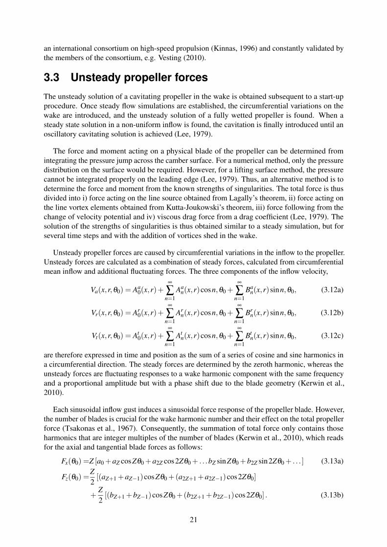
are therefore expressed in time and position as the sum of a series of cosine and sine harmonics ina circumferential direction. The steady forces are determined by the zeroth harmonic, whereas theunsteady forces are fluctuating responses to a wake harmonic component with the same frequencyand a proportional amplitude but with a phase shift due to the blade geometry (Kerwin et al.,2010).

Each sinusoidal inflow gust induces a sinusoidal force response of the propeller blade. However,the number of blades is crucial for the wake harmonic number and their effect on the total propellerforce (Tsakonas et al., 1967). Consequently, the summation of total force only contains thoseharmonics that are integer multiples of the number of blades (Kerwin et al., 2010), which readsfor the axial and tangential blade forces as follows:

Fx(θ0) =Z [a0 +aZ cosZθ0 +a2Z cos2Zθ0 + . . .bZ sinZθ0 +b2Z sin2Zθ0 + . . . ] (3.13a)

Fz(θ0) =Z2[(aZ+1 +aZ−1)cosZθ0 +(a2Z+1 +a2Z−1)cos2Zθ0]

+Z2[(bZ+1 +bZ−1)cosZθ0 +(b2Z+1 +b2Z−1)cos2Zθ0] . (3.13b)

21

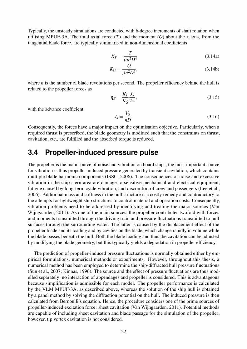
Typically, the unsteady simulations are conducted with 6-degree increments of shaft rotation whenutilising MPUF-3A. The total axial force (T ) and the moment (Q) about the x axis, from thetangential blade force, are typically summarised in non-dimensional coefficients

KT =T

ρn2D4 (3.14a)

KQ =Q

ρn2D5 , (3.14b)

where n is the number of blade revolutions per second. The propeller efficiency behind the hull isrelated to the propeller forces as

ηB =KT

KQ

JS

2π, (3.15)

with the advance coefficientJs =

VS

nD. (3.16)

Consequently, the forces have a major impact on the optimisation objective. Particularly, when arequired thrust is prescribed, the blade geometry is modified such that the constraints on thrust,cavitation, etc., are fulfilled and the absorbed torque is reduced.

3.4 Propeller-induced pressure pulse

The propeller is the main source of noise and vibration on board ships; the most important sourcefor vibration is thus propeller-induced pressure generated by transient cavitation, which containsmultiple blade harmonic components (ISSC, 2006). The consequences of noise and excessivevibration in the ship stern area are damage to sensitive mechanical and electrical equipment,fatigue caused by long-term cycle vibration, and discomfort of crew and passengers (Lee et al.,2006). Additional mass and stiffness in the hull structure is a costly remedy and contradictory tothe attempts for lightweight ship structures to control material and operation costs. Consequently,vibration problems need to be addressed by identifying and treating the major sources (VanWijngaarden, 2011). As one of the main sources, the propeller contributes twofold with forcesand moments transmitted through the driving train and pressure fluctuations transmitted to hullsurfaces through the surrounding water. The latter is caused by the displacement effect of thepropeller blade and its loading and by cavities on the blade, which change rapidly in volume whilethe blade passes beneath the hull. Both the blade loading and thus the cavitation can be adjustedby modifying the blade geometry, but this typically yields a degradation in propeller efficiency.

The prediction of propeller-induced pressure fluctuations is normally obtained either by em-pirical formulations, numerical methods or experiments. However, throughout this thesis, anumerical method has been employed to determine the ship-diffracted hull pressure fluctuations(Sun et al., 2007; Kinnas, 1996). The source and the effect of pressure fluctuations are thus mod-elled separately; no interaction of appendages and propeller is considered. This is advantageousbecause simplification is admissible for each model. The propeller performance is calculatedby the VLM MPUF-3A, as described above, whereas the solution of the ship hull is obtainedby a panel method by solving the diffraction potential on the hull. The induced pressure is thencalculated from Bernoulli’s equation. Hence, the procedure considers one of the prime sources ofpropeller-induced excitation force: sheet cavitation (Van Wijngaarden, 2011). Potential methodsare capable of including sheet cavitation and blade passage for the simulation of the propeller;however, tip vortex cavitation is not considered.

22

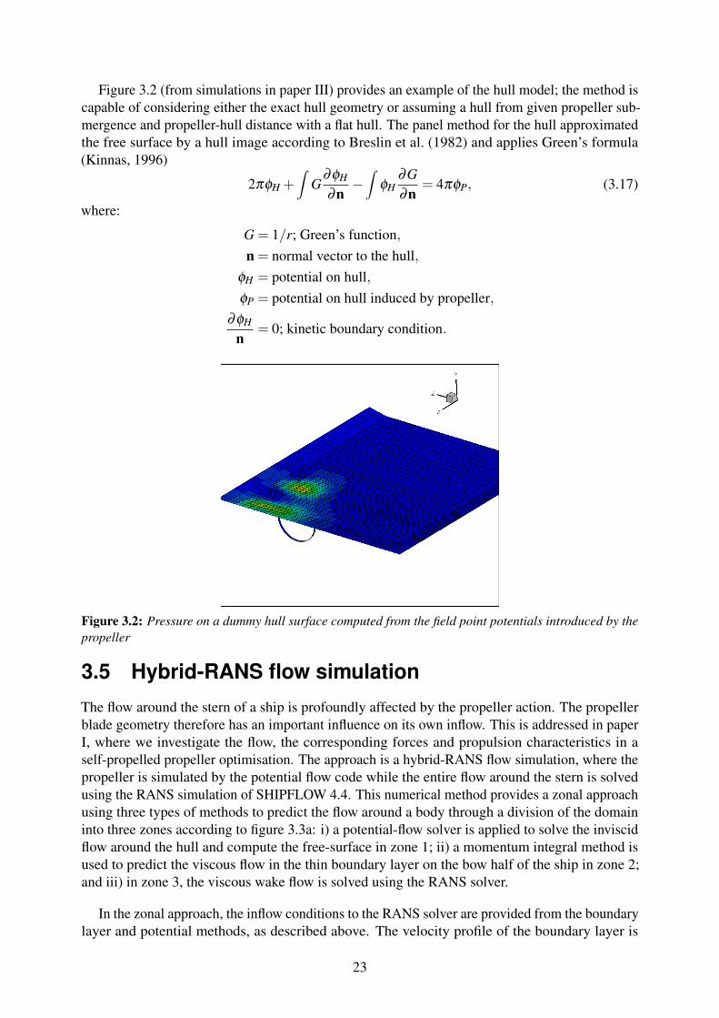
Figure 3.2 (from simulations in paper III) provides an example of the hull model; the method iscapable of considering either the exact hull geometry or assuming a hull from given propeller sub-mergence and propeller-hull distance with a flat hull. The panel method for the hull approximatedthe free surface by a hull image according to Breslin et al. (1982) and applies Green’s formula(Kinnas, 1996)

2πφH +∫

G∂φH

∂n−∫

φH∂G∂n

= 4πφP, (3.17)

where:

G = 1/r; Green’s function,n = normal vector to the hull,

φH = potential on hull,φP = potential on hull induced by propeller,

∂φH

n= 0; kinetic boundary condition.

Figure 3.2: Pressure on a dummy hull surface computed from the field point potentials introduced by thepropeller

3.5 Hybrid-RANS flow simulation

The flow around the stern of a ship is profoundly affected by the propeller action. The propellerblade geometry therefore has an important influence on its own inflow. This is addressed in paperI, where we investigate the flow, the corresponding forces and propulsion characteristics in aself-propelled propeller optimisation. The approach is a hybrid-RANS flow simulation, where thepropeller is simulated by the potential flow code while the entire flow around the stern is solvedusing the RANS simulation of SHIPFLOW 4.4. This numerical method provides a zonal approachusing three types of methods to predict the flow around a body through a division of the domaininto three zones according to figure 3.3a: i) a potential-flow solver is applied to solve the inviscidflow around the hull and compute the free-surface in zone 1; ii) a momentum integral method isused to predict the viscous flow in the thin boundary layer on the bow half of the ship in zone 2;and iii) in zone 3, the viscous wake flow is solved using the RANS solver.

In the zonal approach, the inflow conditions to the RANS solver are provided from the boundarylayer and potential methods, as described above. The velocity profile of the boundary layer is

23

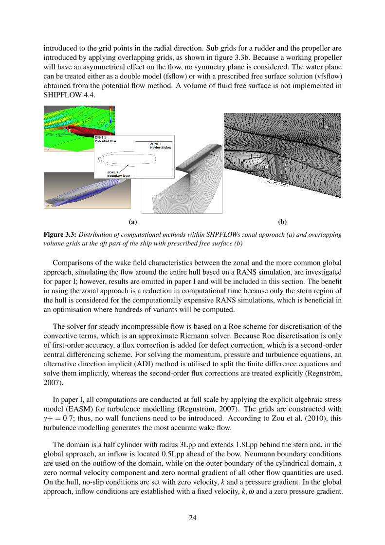
introduced to the grid points in the radial direction. Sub grids for a rudder and the propeller areintroduced by applying overlapping grids, as shown in figure 3.3b. Because a working propellerwill have an asymmetrical effect on the flow, no symmetry plane is considered. The water planecan be treated either as a double model (fsflow) or with a prescribed free surface solution (vfsflow)obtained from the potential flow method. A volume of fluid free surface is not implemented inSHIPFLOW 4.4.

(a) (b)

Figure 3.3: Distribution of computational methods within SHPFLOWs zonal approach (a) and overlappingvolume grids at the aft part of the ship with prescribed free surface (b)

Comparisons of the wake field characteristics between the zonal and the more common globalapproach, simulating the flow around the entire hull based on a RANS simulation, are investigatedfor paper I; however, results are omitted in paper I and will be included in this section. The benefitin using the zonal approach is a reduction in computational time because only the stern region ofthe hull is considered for the computationally expensive RANS simulations, which is beneficial inan optimisation where hundreds of variants will be computed.

The solver for steady incompressible flow is based on a Roe scheme for discretisation of theconvective terms, which is an approximate Riemann solver. Because Roe discretisation is onlyof first-order accuracy, a flux correction is added for defect correction, which is a second-ordercentral differencing scheme. For solving the momentum, pressure and turbulence equations, analternative direction implicit (ADI) method is utilised to split the finite difference equations andsolve them implicitly, whereas the second-order flux corrections are treated explicitly (Regnstrom,2007).

In paper I, all computations are conducted at full scale by applying the explicit algebraic stressmodel (EASM) for turbulence modelling (Regnstrom, 2007). The grids are constructed withy+ = 0.7; thus, no wall functions need to be introduced. According to Zou et al. (2010), thisturbulence modelling generates the most accurate wake flow.

The domain is a half cylinder with radius 3Lpp and extends 1.8Lpp behind the stern and, in theglobal approach, an inflow is located 0.5Lpp ahead of the bow. Neumann boundary conditionsare used on the outflow of the domain, while on the outer boundary of the cylindrical domain, azero normal velocity component and zero normal gradient of all other flow quantities are used.On the hull, no-slip conditions are set with zero velocity, k and a pressure gradient. In the globalapproach, inflow conditions are established with a fixed velocity, k,ω and a zero pressure gradient.

24

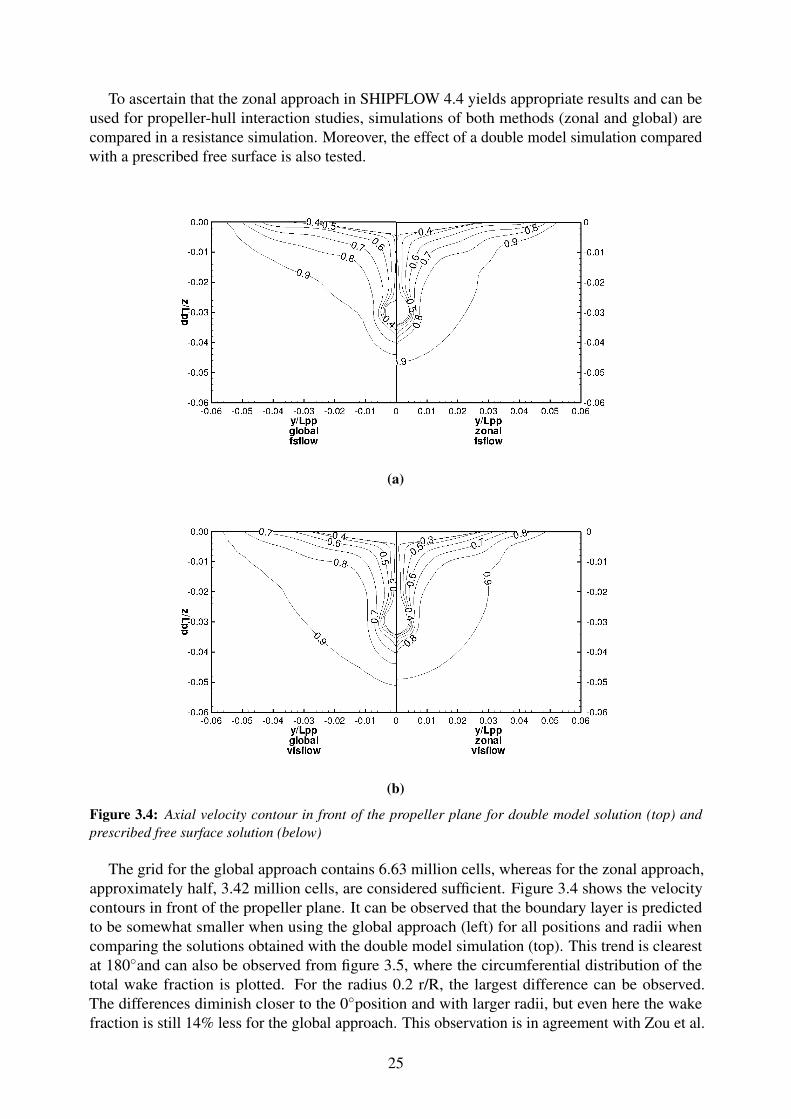
To ascertain that the zonal approach in SHIPFLOW 4.4 yields appropriate results and can beused for propeller-hull interaction studies, simulations of both methods (zonal and global) arecompared in a resistance simulation. Moreover, the effect of a double model simulation comparedwith a prescribed free surface is also tested.

(a)

(b)

Figure 3.4: Axial velocity contour in front of the propeller plane for double model solution (top) andprescribed free surface solution (below)

The grid for the global approach contains 6.63 million cells, whereas for the zonal approach,approximately half, 3.42 million cells, are considered sufficient. Figure 3.4 shows the velocitycontours in front of the propeller plane. It can be observed that the boundary layer is predictedto be somewhat smaller when using the global approach (left) for all positions and radii whencomparing the solutions obtained with the double model simulation (top). This trend is clearestat 180◦and can also be observed from figure 3.5, where the circumferential distribution of thetotal wake fraction is plotted. For the radius 0.2 r/R, the largest difference can be observed.The differences diminish closer to the 0◦position and with larger radii, but even here the wakefraction is still 14% less for the global approach. This observation is in agreement with Zou et al.

25

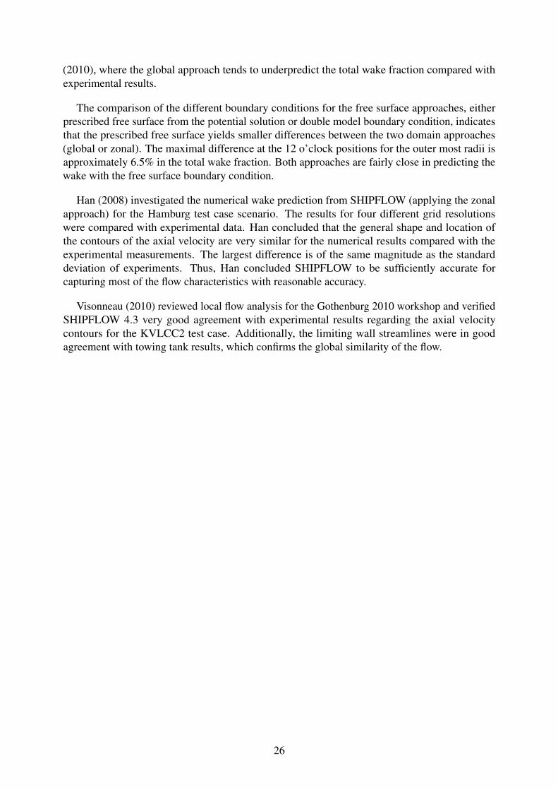
(2010), where the global approach tends to underpredict the total wake fraction compared withexperimental results.

The comparison of the different boundary conditions for the free surface approaches, eitherprescribed free surface from the potential solution or double model boundary condition, indicatesthat the prescribed free surface yields smaller differences between the two domain approaches(global or zonal). The maximal difference at the 12 o’clock positions for the outer most radii isapproximately 6.5% in the total wake fraction. Both approaches are fairly close in predicting thewake with the free surface boundary condition.

Han (2008) investigated the numerical wake prediction from SHIPFLOW (applying the zonalapproach) for the Hamburg test case scenario. The results for four different grid resolutionswere compared with experimental data. Han concluded that the general shape and location ofthe contours of the axial velocity are very similar for the numerical results compared with theexperimental measurements. The largest difference is of the same magnitude as the standarddeviation of experiments. Thus, Han concluded SHIPFLOW to be sufficiently accurate forcapturing most of the flow characteristics with reasonable accuracy.

Visonneau (2010) reviewed local flow analysis for the Gothenburg 2010 workshop and verifiedSHIPFLOW 4.3 very good agreement with experimental results regarding the axial velocitycontours for the KVLCC2 test case. Additionally, the limiting wall streamlines were in goodagreement with towing tank results, which confirms the global similarity of the flow.

26

Total

wakefraction

(wt)

(a)

Total

wakefraction

(wt)

(b)

Figure 3.5: Axial velocity contour in front of the propeller plane for double model solution (top) andprescribed free surface solution (below)

27

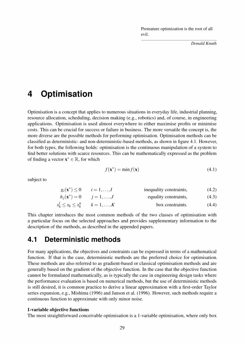
Premature optimization is the root of allevil.

Donald Knuth

4 Optimisation

Optimisation is a concept that applies to numerous situations in everyday life, industrial planning,resource allocation, scheduling, decision making (e.g., robotics) and, of course, in engineeringapplications. Optimisation is used almost everywhere to either maximise profits or minimisecosts. This can be crucial for success or failure in business. The more versatile the concept is, themore diverse are the possible methods for performing optimisation. Optimisation methods can beclassified as deterministic- and non-deterministic-based methods, as shown in figure 4.1. However,for both types, the following holds: optimisation is the continuous manipulation of a system tofind better solutions with scarce resources. This can be mathematically expressed as the problemof finding a vector x∗ ∈ R, for which

f (x∗) = min f (x) (4.1)

subject to

gi(x∗)≤ 0 i = 1, . . . , I inequality constraints, (4.2)h j(x∗) = 0 j = 1, . . . ,J equality constraints, (4.3)

xlk ≤ xk ≤ xu

k k = 1, . . . ,K box constraints. (4.4)

This chapter introduces the most common methods of the two classes of optimisation witha particular focus on the selected approaches and provides supplementary information to thedescription of the methods, as described in the appended papers.

4.1 Deterministic methods

For many applications, the objectives and constraints can be expressed in terms of a mathematicalfunction. If that is the case, deterministic methods are the preferred choice for optimisation.These methods are also referred to as gradient-based or classical optimisation methods and aregenerally based on the gradient of the objective function. In the case that the objective functioncannot be formulated mathematically, as is typically the case in engineering design tasks wherethe performance evaluation is based on numerical methods, but the use of deterministic methodsis still desired, it is common practice to derive a linear approximation with a first-order Taylorseries expansion, e.g., Mishima (1996) and Janson et al. (1996). However, such methods require acontinuous function to approximate with only minor noise.

1-variable objective functionsThe most straightforward conceivable optimisation is a 1-variable optimisation, where only box

29

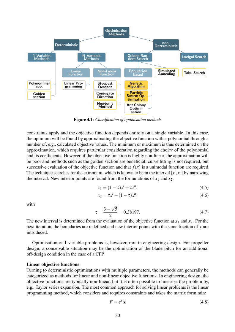
OptimisationMethods

Deterministicnon-

Deterministic

1-VariableMethods

N-VariableMethods

Polynominalapp.

Goldensection

LinearFunction

Non-LinearFunction

Linear Pro-gramming

SteepestDescent

ConjugateDirection

Newton’sMethod

Guided Ran-dom Search Locigal Search

Populationbased Tabu SearchSimulated

Annealing

GeneticAlgorithm

ParticleSwarm Op-timisation

Ant ColonyOptimi-sation

Figure 4.1: Classification of optimisation methods

constraints apply and the objective function depends entirely on a single variable. In this case,the optimum will be found by approximating the objective function with a polynomial through anumber of, e.g., calculated objective values. The minimum or maximum is thus determined on theapproximation, which requires particular consideration regarding the choice of the polynomialand its coefficients. However, if the objective function is highly non-linear, the approximation willbe poor and methods such as the golden section are beneficial; curve fitting is not required, butsuccessive evaluation of the objective function and that f (x) is a unimodal function are required.The technique searches for the extremum, which is known to be in the interval [xl,xu] by narrowingthe interval. New interior points are found from the formulations of x1 and x2,

x1 = (1− τ)xl + τxu, (4.5)

x2 = τxl +(1− τ)xu, (4.6)

with

τ =3−√

52

= 0.38197. (4.7)

The new interval is determined from the evaluation of the objective function at x1 and x2. For thenext iteration, the boundaries are redefined and new interior points with the same fraction of τ areintroduced.

Optimisation of 1-variable problems is, however, rare in engineering design. For propellerdesign, a conceivable situation may be the optimisation of the blade pitch for an additionaloff-design condition in the case of a CPP.

Linear objective functionsTurning to deterministic optimisations with multiple parameters, the methods can generally becategorized as methods for linear and non-linear objective functions. In engineering design, theobjective functions are typically non-linear, but it is often possible to linearise the problem by,e.g., Taylor series expansion. The most common approach for solving linear problems is the linearprogramming method, which considers and requires constraints and takes the matrix form min:

F = cT x (4.8)

30

subject to:

Ax = b (4.9)xi ≥ 0 i = 1, . . . ,n (4.10)

where c contains the cost coefficients, x are the decision variables, A is a matrix for all constraintequation coefficients, and vector b contains the constraints (Vanderplaats, 2001). There are severalalgorithms available for solving the linear system of equations, of which the simplex method isthe most famous.

Non-linear objective functionsThe most common optimisation problems are of the type of non-linear objective functions andcan only be solved iteratively from a starting point, with interrogation of the objective function’sgradient. The general optimisation strategy is the same for the methods listed in figure 4.1,

xi+1 = xi +α∗si, (4.11)

where xi is the current point, the vector si is the search direction to the next location, and α is ascalar for the step size of the movement in the search direction. The gradient ∇ f (xi) is calculatedto determine the search direction si =−∇ f (xi), which yields the next location xi+1. The step sizeα∗ represents the optimal step size for the current search direction. The determination is in itself a1-variable optimisation problem. Equation 4.11 outlines the first-order method steepest descent,which only uses the first derivative of f . The conjugate direction method is also of the first-ordertype, but it modifies the search direction based on the concept of conjugate direction, defined as

si+1 =−∇ f (xi)+βisi (4.12)

with

βi =‖∇ f (xi+1)‖2

‖∇ f (xi)‖2 . (4.13)

This method dramatically improves the steepest descent in terms of convergence rate and is usuallyapplied following a steepest descent optimisation (Vanderplaats, 2001).

Second-order methods also use the information of the second derivative of the objective functionto derive the search direction. The second derivative determines whether a stationary point at xis a minimum. In the general n-dimensional case, the second derivative is given by the Hessianmatrix H, which is positive definite in the case of a minimum at x. The search direction derivedby Newton’s method then reads as

si =−∇ f (xi)

∇2 f (xi). (4.14)

Algorithms commonly used to solve non-linear optimisation problems are typically based oneither one of the listed methods, e.g., the Gauss-Newton algorithm or the Levenberg-Marquardtalgorithm. The advantage of these methods is clearly a good convergence; provided that theobjective function is quadratic and convex, Newton’s methods, for instance, require only oneiteration to find the optimum (Vanderplaats, 2001). However, the calculation of the first andsecond derivatives of the objective function can become very expensive. More problems ariseif the objective function is noisy or if constraints are to be applied because the derivative ofeach constraint function is also required. An alternative deterministic approach utilises sensitivityderivatives of the objective function with respect to the decision variables to determine the direction

31

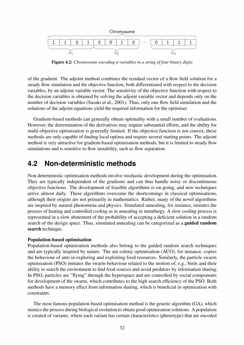
1 1 0 1 0 0 1 0 · · · 0 1 1 1

x1 xnx2

Chromosome

Figure 4.2: Chromosome encoding n variables in a string of four binary digits

of the gradient. The adjoint method combines the residual vector of a flow field solution for asteady flow simulation and the objective function, both differentiated with respect to the decisionvariables, by an adjoint variable vector. The sensitivity of the objective function with respect tothe decision variables is obtained by solving the adjoint variable vector and depends only on thenumber of decision variables (Sasaki et al., 2001). Thus, only one flow field simulation and thesolutions of the adjoint equations yield the required information for the optimiser.

Gradient-based methods can generally obtain optimality with a small number of evaluations.However, the determination of the derivatives may require substantial efforts, and the ability formulti-objective optimisation is generally limited. If the objective function is not convex, thesemethods are only capable of finding local optima and require several starting points. The adjointmethod is very attractive for gradient-based optimisation methods, but it is limited to steady flowsimulations and is sensitive to flow instability, such as flow separation.

4.2 Non-deterministic methods

Non-deterministic optimisation methods involve stochastic development during the optimisation.They are typically independent of the gradients and can thus handle noisy or discontinuousobjective functions. The development of feasible algorithms is on-going, and new techniquesarrive almost daily. These algorithms overcome the shortcomings in classical optimisations,although their origins are not primarily in mathematics. Rather, many of the novel algorithmsare inspired by natural phenomena and physics. Simulated annealing, for instance, imitates theprocess of heating and controlled cooling as in annealing in metallurgy. A slow cooling process isrepresented in a slow abatement of the probability of accepting a deficient solution in a randomsearch of the design space. Thus, simulated annealing can be categorized as a guided randomsearch technique.

Population-based optimisationPopulation-based optimisation methods also belong to the guided random search techniquesand are typically inspired by nature. The ant colony optimisation (ACO), for instance, copiesthe behaviour of ants in exploring and exploiting food resources. Similarly, the particle swarmoptimisation (PSO) imitates the swarm behaviour related to the motion of, e.g., birds and theirability to search the environment to find food sources and avoid predators by information sharing.In PSO, particles are ”flying” through the hyperspace and are controlled by social componentsfor development of the swarm, which contributes to the high search efficiency of the PSO. Bothmethods have a memory effect from information sharing, which is beneficial in optimisation withconstraints.

The most famous population-based optimisation method is the genetic algorithm (GA), whichmimics the process during biological evolution to obtain good optimisation solutions. A populationis created of variants, where each variant has certain characteristics (phenotype) that are encoded

32

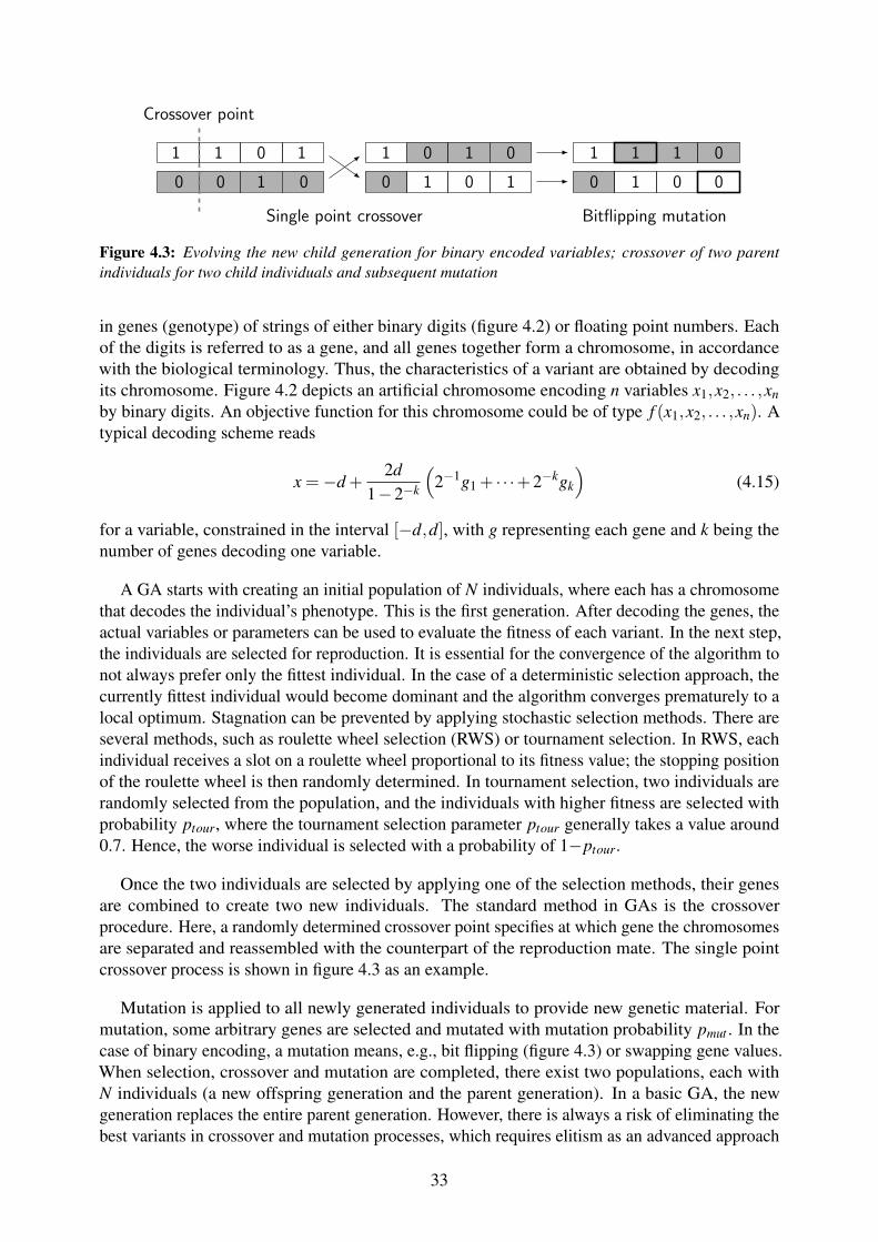
1 1 0 1

0 0 1 0

1 0 1 0

0 1 0 1

Crossover point

Single point crossover

1 11 0

0 1 0 0

Bitflipping mutation

Figure 4.3: Evolving the new child generation for binary encoded variables; crossover of two parentindividuals for two child individuals and subsequent mutation

in genes (genotype) of strings of either binary digits (figure 4.2) or floating point numbers. Eachof the digits is referred to as a gene, and all genes together form a chromosome, in accordancewith the biological terminology. Thus, the characteristics of a variant are obtained by decodingits chromosome. Figure 4.2 depicts an artificial chromosome encoding n variables x1,x2, . . . ,xnby binary digits. An objective function for this chromosome could be of type f (x1,x2, . . . ,xn). Atypical decoding scheme reads

x =−d +2d

1−2−k

(2−1g1 + · · ·+2−kgk

)(4.15)

for a variable, constrained in the interval [−d,d], with g representing each gene and k being thenumber of genes decoding one variable.

A GA starts with creating an initial population of N individuals, where each has a chromosomethat decodes the individual’s phenotype. This is the first generation. After decoding the genes, theactual variables or parameters can be used to evaluate the fitness of each variant. In the next step,the individuals are selected for reproduction. It is essential for the convergence of the algorithm tonot always prefer only the fittest individual. In the case of a deterministic selection approach, thecurrently fittest individual would become dominant and the algorithm converges prematurely to alocal optimum. Stagnation can be prevented by applying stochastic selection methods. There areseveral methods, such as roulette wheel selection (RWS) or tournament selection. In RWS, eachindividual receives a slot on a roulette wheel proportional to its fitness value; the stopping positionof the roulette wheel is then randomly determined. In tournament selection, two individuals arerandomly selected from the population, and the individuals with higher fitness are selected withprobability ptour, where the tournament selection parameter ptour generally takes a value around0.7. Hence, the worse individual is selected with a probability of 1−ptour.

Once the two individuals are selected by applying one of the selection methods, their genesare combined to create two new individuals. The standard method in GAs is the crossoverprocedure. Here, a randomly determined crossover point specifies at which gene the chromosomesare separated and reassembled with the counterpart of the reproduction mate. The single pointcrossover process is shown in figure 4.3 as an example.

Mutation is applied to all newly generated individuals to provide new genetic material. Formutation, some arbitrary genes are selected and mutated with mutation probability pmut . In thecase of binary encoding, a mutation means, e.g., bit flipping (figure 4.3) or swapping gene values.When selection, crossover and mutation are completed, there exist two populations, each withN individuals (a new offspring generation and the parent generation). In a basic GA, the newgeneration replaces the entire parent generation. However, there is always a risk of eliminating thebest variants in crossover and mutation processes, which requires elitism as an advanced approach

33

to maintain already good individuals. In elitism, a few exact copies of the best individuals areselected from the parent generation and placed in the new generation.

Binary encoding of genes features specific characteristics of an implicit probability distributionand characteristics of creating both expanding or contracting crossover (children solutions outsideand inside the bounded region by two parents), which is simulated in real value encoding, e.g.,by simulated binary crossover (SBX) (Deb et al., 1995). The method presents a spread factor,defined as a non-dimensional ratio of the distance between the two children (c1,c2) and twoparents (p1, p2) in parameter space

β = ‖ c1− c2

p1− p2‖. (4.16)

A probability distribution function P(β ) is introduced that depends not only on the spread factorbut also on a distribution index n

P(β ) =

{0.5(n+1)β n, if β ≤ 1;0.5(n+1) 1

β n+2 , otherwise,(4.17)

which determines where to create the new child solutions due to crossover. Thus, β ′ is determinedfrom a random number u as the cumulative probability

∫ β ′

0P(β )dβ = u. (4.18)

In figure 4.4a, the probability distribution is provided for different distribution indices n andfor only one side of the boundary region; a β of 1 corresponds the location of the parent, andaccordingly, β ≤ 1 corresponds to a contraction and β > 1 corresponds to an expansion.

The simulated binary mutation is obtained similarly. The value of one input variable is perturbedby a mutation operator using a polynomial probability distribution (Deb et al., 1996). The mutatedvalue is calculated with the probability distribution

P(δ ) = 0.5(n+1)(1−δ )n, (4.19)

a random number u and the cumulative probability. Figure 4.4b shows different probabilitydistributions, depending on the distribution index n. The mutated value is finally calculated withthe maximum perturbation ∆max as

c = p+δ ′∆max. (4.20)

Thus far, the general genetic algorithm considered only a single objective function for fitnessevaluation. However, in some cases, the system must meet more than one objective simultaneously.In such cases, the mathematical description (eqn. 4.1) becomes

min fl(x) l = 1, . . . ,L (4.21)

and a unique solution cannot be identified that simultaneously leads to the optimum in all objectives.A number of methods exist to overcome the problem of possibly conflicting objectives. Theclassical approach is weighting each objective in a linear combination to become a utility objective

34

-

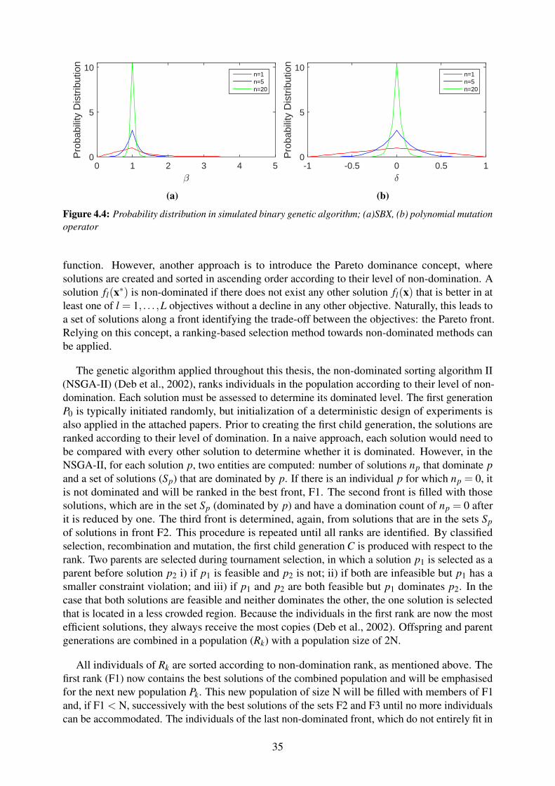
0 1 2 3 4 5

Pro

babi

lity

Dis

trib

utio

n

0

5

10n=1n=5n=20

(a)

/

-1 -0.5 0 0.5 1

Pro

babi

lity

Dis

trib

utio

n

0

5

10n=1n=5n=20

(b)

Figure 4.4: Probability distribution in simulated binary genetic algorithm; (a)SBX, (b) polynomial mutationoperator

function. However, another approach is to introduce the Pareto dominance concept, wheresolutions are created and sorted in ascending order according to their level of non-domination. Asolution fl(x∗) is non-dominated if there does not exist any other solution fl(x) that is better in atleast one of l = 1, . . . ,L objectives without a decline in any other objective. Naturally, this leads toa set of solutions along a front identifying the trade-off between the objectives: the Pareto front.Relying on this concept, a ranking-based selection method towards non-dominated methods canbe applied.

The genetic algorithm applied throughout this thesis, the non-dominated sorting algorithm II(NSGA-II) (Deb et al., 2002), ranks individuals in the population according to their level of non-domination. Each solution must be assessed to determine its dominated level. The first generationP0 is typically initiated randomly, but initialization of a deterministic design of experiments isalso applied in the attached papers. Prior to creating the first child generation, the solutions areranked according to their level of domination. In a naive approach, each solution would need tobe compared with every other solution to determine whether it is dominated. However, in theNSGA-II, for each solution p, two entities are computed: number of solutions np that dominate pand a set of solutions (Sp) that are dominated by p. If there is an individual p for which np = 0, itis not dominated and will be ranked in the best front, F1. The second front is filled with thosesolutions, which are in the set Sp (dominated by p) and have a domination count of np = 0 afterit is reduced by one. The third front is determined, again, from solutions that are in the sets Spof solutions in front F2. This procedure is repeated until all ranks are identified. By classifiedselection, recombination and mutation, the first child generation C is produced with respect to therank. Two parents are selected during tournament selection, in which a solution p1 is selected as aparent before solution p2 i) if p1 is feasible and p2 is not; ii) if both are infeasible but p1 has asmaller constraint violation; and iii) if p1 and p2 are both feasible but p1 dominates p2. In thecase that both solutions are feasible and neither dominates the other, the one solution is selectedthat is located in a less crowded region. Because the individuals in the first rank are now the mostefficient solutions, they always receive the most copies (Deb et al., 2002). Offspring and parentgenerations are combined in a population (Rk) with a population size of 2N.

All individuals of Rk are sorted according to non-domination rank, as mentioned above. Thefirst rank (F1) now contains the best solutions of the combined population and will be emphasisedfor the next new population Pk. This new population of size N will be filled with members of F1and, if F1 < N, successively with the best solutions of the sets F2 and F3 until no more individualscan be accommodated. The individuals of the last non-dominated front, which do not entirely fit in

35

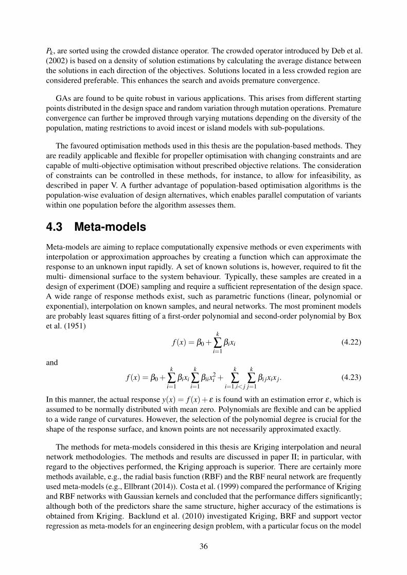
Pk, are sorted using the crowded distance operator. The crowded operator introduced by Deb et al.(2002) is based on a density of solution estimations by calculating the average distance betweenthe solutions in each direction of the objectives. Solutions located in a less crowded region areconsidered preferable. This enhances the search and avoids premature convergence.

GAs are found to be quite robust in various applications. This arises from different startingpoints distributed in the design space and random variation through mutation operations. Prematureconvergence can further be improved through varying mutations depending on the diversity of thepopulation, mating restrictions to avoid incest or island models with sub-populations.

The favoured optimisation methods used in this thesis are the population-based methods. Theyare readily applicable and flexible for propeller optimisation with changing constraints and arecapable of multi-objective optimisation without prescribed objective relations. The considerationof constraints can be controlled in these methods, for instance, to allow for infeasibility, asdescribed in paper V. A further advantage of population-based optimisation algorithms is thepopulation-wise evaluation of design alternatives, which enables parallel computation of variantswithin one population before the algorithm assesses them.

4.3 Meta-models

Meta-models are aiming to replace computationally expensive methods or even experiments withinterpolation or approximation approaches by creating a function which can approximate theresponse to an unknown input rapidly. A set of known solutions is, however, required to fit themulti- dimensional surface to the system behaviour. Typically, these samples are created in adesign of experiment (DOE) sampling and require a sufficient representation of the design space.A wide range of response methods exist, such as parametric functions (linear, polynomial orexponential), interpolation on known samples, and neural networks. The most prominent modelsare probably least squares fitting of a first-order polynomial and second-order polynomial by Boxet al. (1951)

f (x) = β0 +k

∑i=1

βixi (4.22)

and

f (x) = β0 +k

∑i=1

βixi

k

∑i=1

βiix2i +

k

∑i=1,i< j

k

∑j=1

βi jxix j. (4.23)

In this manner, the actual response y(x) = f (x)+ ε is found with an estimation error ε , which isassumed to be normally distributed with mean zero. Polynomials are flexible and can be appliedto a wide range of curvatures. However, the selection of the polynomial degree is crucial for theshape of the response surface, and known points are not necessarily approximated exactly.

The methods for meta-models considered in this thesis are Kriging interpolation and neuralnetwork methodologies. The methods and results are discussed in paper II; in particular, withregard to the objectives performed, the Kriging approach is superior. There are certainly moremethods available, e.g., the radial basis function (RBF) and the RBF neural network are frequentlyused meta-models (e.g., Ellbrant (2014)). Costa et al. (1999) compared the performance of Krigingand RBF networks with Gaussian kernels and concluded that the performance differs significantly;although both of the predictors share the same structure, higher accuracy of the estimations isobtained from Kriging. Backlund et al. (2010) investigated Kriging, BRF and support vectorregression as meta-models for an engineering design problem, with a particular focus on the model

36

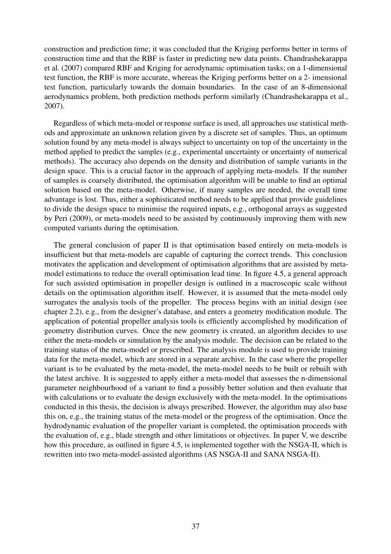
construction and prediction time; it was concluded that the Kriging performs better in terms ofconstruction time and that the RBF is faster in predicting new data points. Chandrashekarappaet al. (2007) compared RBF and Kriging for aerodynamic optimisation tasks; on a 1-dimensionaltest function, the RBF is more accurate, whereas the Kriging performs better on a 2- imensionaltest function, particularly towards the domain boundaries. In the case of an 8-dimensionalaerodynamics problem, both prediction methods perform similarly (Chandrashekarappa et al.,2007).

Regardless of which meta-model or response surface is used, all approaches use statistical meth-ods and approximate an unknown relation given by a discrete set of samples. Thus, an optimumsolution found by any meta-model is always subject to uncertainty on top of the uncertainty in themethod applied to predict the samples (e.g., experimental uncertainty or uncertainty of numericalmethods). The accuracy also depends on the density and distribution of sample variants in thedesign space. This is a crucial factor in the approach of applying meta-models. If the numberof samples is coarsely distributed, the optimisation algorithm will be unable to find an optimalsolution based on the meta-model. Otherwise, if many samples are needed, the overall timeadvantage is lost. Thus, either a sophisticated method needs to be applied that provide guidelinesto divide the design space to minimise the required inputs, e.g., orthogonal arrays as suggestedby Peri (2009), or meta-models need to be assisted by continuously improving them with newcomputed variants during the optimisation.

The general conclusion of paper II is that optimisation based entirely on meta-models isinsufficient but that meta-models are capable of capturing the correct trends. This conclusionmotivates the application and development of optimisation algorithms that are assisted by meta-model estimations to reduce the overall optimisation lead time. In figure 4.5, a general approachfor such assisted optimisation in propeller design is outlined in a macroscopic scale withoutdetails on the optimisation algorithm itself. However, it is assumed that the meta-model onlysurrogates the analysis tools of the propeller. The process begins with an initial design (seechapter 2.2), e.g., from the designer’s database, and enters a geometry modification module. Theapplication of potential propeller analysis tools is efficiently accomplished by modification ofgeometry distribution curves. Once the new geometry is created, an algorithm decides to useeither the meta-models or simulation by the analysis module. The decision can be related to thetraining status of the meta-model or prescribed. The analysis module is used to provide trainingdata for the meta-model, which are stored in a separate archive. In the case where the propellervariant is to be evaluated by the meta-model, the meta-model needs to be built or rebuilt withthe latest archive. It is suggested to apply either a meta-model that assesses the n-dimensionalparameter neighbourhood of a variant to find a possibly better solution and then evaluate thatwith calculations or to evaluate the design exclusively with the meta-model. In the optimisationsconducted in this thesis, the decision is always prescribed. However, the algorithm may also basethis on, e.g., the training status of the meta-model or the progress of the optimisation. Once thehydrodynamic evaluation of the propeller variant is completed, the optimisation proceeds withthe evaluation of, e.g., blade strength and other limitations or objectives. In paper V, we describehow this procedure, as outlined in figure 4.5, is implemented together with the NSGA-II, which isrewritten into two meta-model-assisted algorithms (AS NSGA-II and SANA NSGA-II).

37

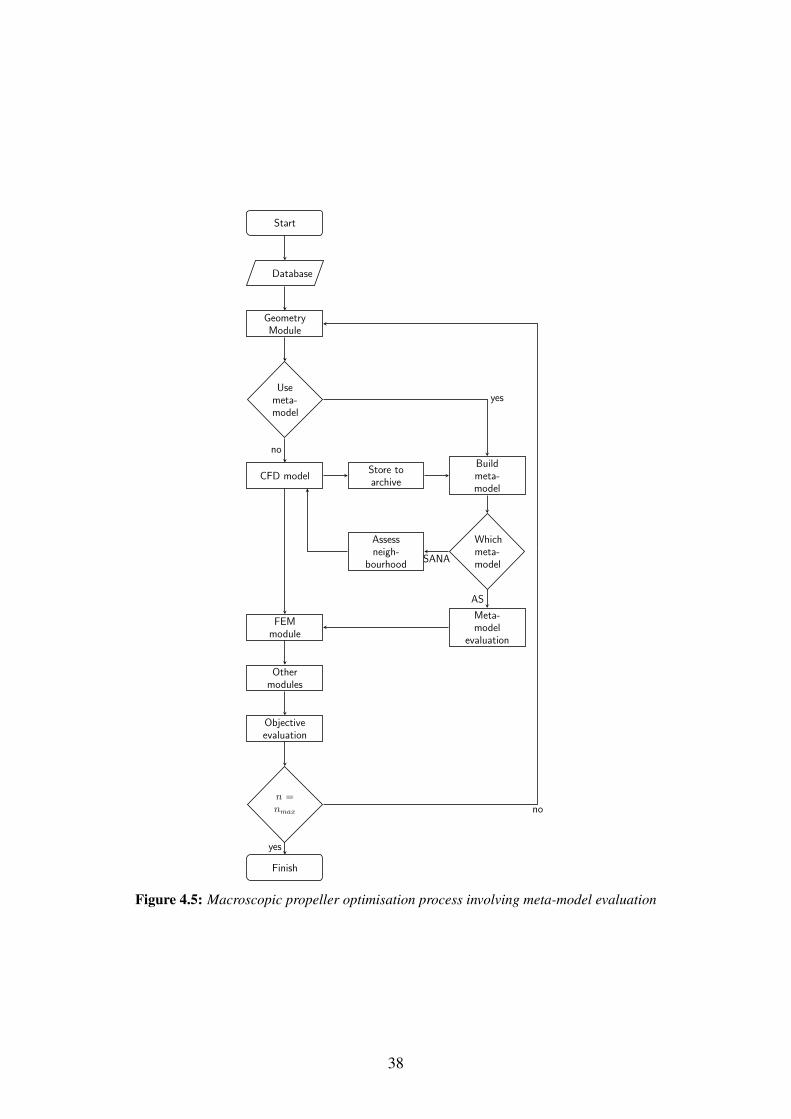
Start

Database

GeometryModule

Usemeta-model

CFD modelStore toarchive

Buildmeta-model

Whichmeta-model

Meta-model

evaluation

Assessneigh-

bourhood

FEMmodule

Othermodules

Objectiveevaluation

n =nmax

yes

no

AS

SANA

no

Finish

yes

Figure 4.5: Macroscopic propeller optimisation process involving meta-model evaluation

38

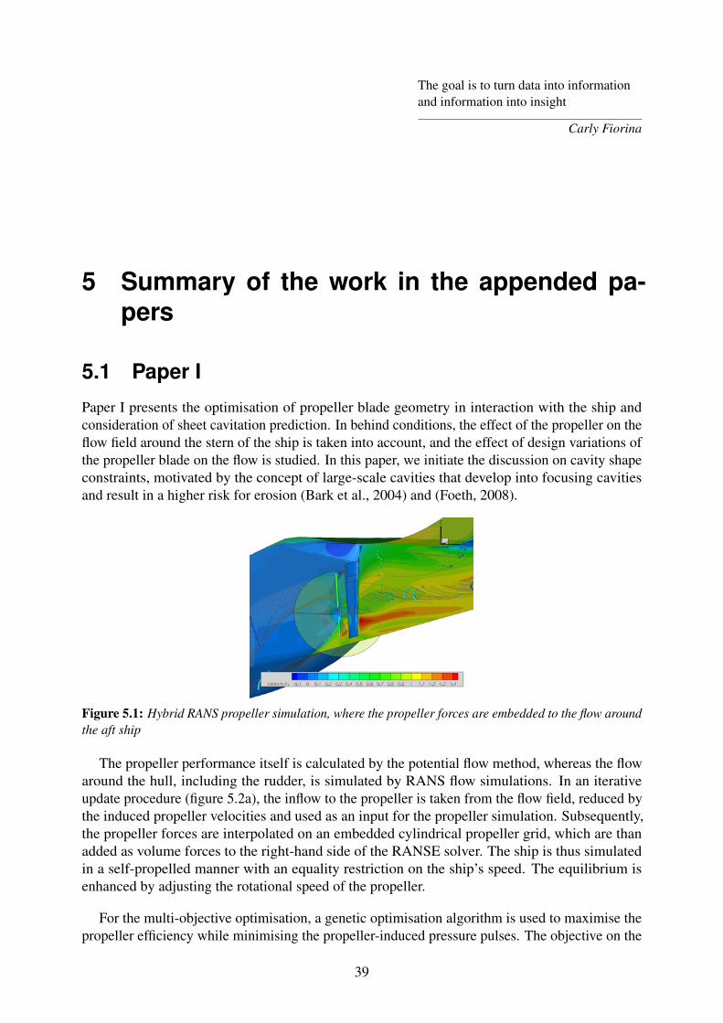
The goal is to turn data into informationand information into insight

Carly Fiorina

5 Summary of the work in the appended pa-pers

5.1 Paper I

Paper I presents the optimisation of propeller blade geometry in interaction with the ship andconsideration of sheet cavitation prediction. In behind conditions, the effect of the propeller on theflow field around the stern of the ship is taken into account, and the effect of design variations ofthe propeller blade on the flow is studied. In this paper, we initiate the discussion on cavity shapeconstraints, motivated by the concept of large-scale cavities that develop into focusing cavitiesand result in a higher risk for erosion (Bark et al., 2004) and (Foeth, 2008).

Figure 5.1: Hybrid RANS propeller simulation, where the propeller forces are embedded to the flow aroundthe aft ship

The propeller performance itself is calculated by the potential flow method, whereas the flowaround the hull, including the rudder, is simulated by RANS flow simulations. In an iterativeupdate procedure (figure 5.2a), the inflow to the propeller is taken from the flow field, reduced bythe induced propeller velocities and used as an input for the propeller simulation. Subsequently,the propeller forces are interpolated on an embedded cylindrical propeller grid, which are thanadded as volume forces to the right-hand side of the RANSE solver. The ship is thus simulatedin a self-propelled manner with an equality restriction on the ship’s speed. The equilibrium isenhanced by adjusting the rotational speed of the propeller.

For the multi-objective optimisation, a genetic optimisation algorithm is used to maximise thepropeller efficiency while minimising the propeller-induced pressure pulses. The objective on the

39

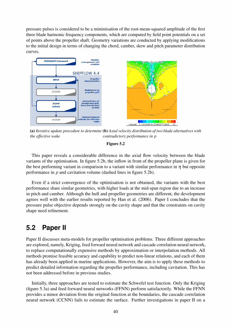
pressure pulses is considered to be a minimisation of the root-mean-squared amplitude of the firstthree blade harmonic frequency components, which are computed by field point potentials on a setof points above the propeller shaft. Geometry variations are conducted by applying modificationsto the initial design in terms of changing the chord, camber, skew and pitch parameter distributioncurves.

(a) Iterative update procedure to determinethe effective wake

(b) Axial velocity distribution of two blade alternatives withcontradictory performance in p

Figure 5.2

This paper reveals a considerable difference in the axial flow velocity between the bladevariants of the optimisation. In figure 5.2b, the inflow in front of the propeller plane is given forthe best performing variant in comparison to a variant with similar performance in η but oppositeperformance in p and cavitation volume (dashed lines in figure 5.2b).

Even if a strict convergence of the optimisation is not obtained, the variants with the bestperformance share similar geometries, with higher loads at the mid-span region due to an increasein pitch and camber. Although the hull and propeller geometries are different, the developmentagrees well with the earlier results reported by Han et al. (2006). Paper I concludes that thepressure pulse objective depends strongly on the cavity shape and that the constraints on cavityshape need refinement.

5.2 Paper II

Paper II discusses meta-models for propeller optimisation problems. Three different approachesare explored, namely, Kriging, feed forward neural network and cascade correlation neural network,to replace computationally expensive methods by approximation or interpolation methods. Allmethods promise feasible accuracy and capability to predict non-linear relations, and each of themhas already been applied in marine applications. However, the aim is to apply these methods topredict detailed information regarding the propeller performance, including cavitation. This hasnot been addressed before in previous studies.

Initially, three approaches are tested to estimate the Schwefel test function. Only the Kriging(figure 5.3a) and feed forward neural networks (FFNN) perform satisfactorily. While the FFNNprovides a minor deviation from the original function at the boundaries, the cascade correlationneural network (CCNN) fails to estimate the surface. Further investigations in paper II on a

40

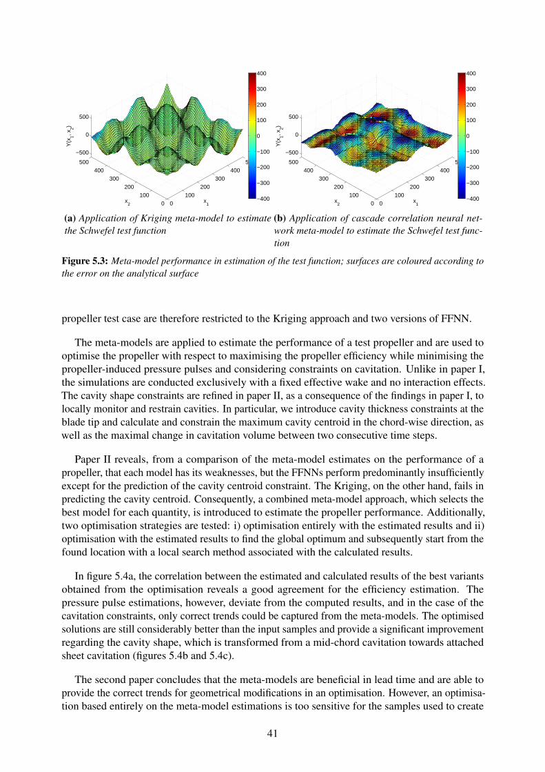
0100

200300

400500

0100

200300

400500

−500

0

500

x1

x2

Y(x

1, x2)

−400

−300

−200

−100

0

100

200

300

400

(a) Application of Kriging meta-model to estimatethe Schwefel test function

0100

200300

400500

0100

200300

400500

−500

0

500

x1

x2

Y(x

1, x2)

−400

−300

−200

−100

0

100

200

300

400

(b) Application of cascade correlation neural net-work meta-model to estimate the Schwefel test func-tion

Figure 5.3: Meta-model performance in estimation of the test function; surfaces are coloured according tothe error on the analytical surface

propeller test case are therefore restricted to the Kriging approach and two versions of FFNN.

The meta-models are applied to estimate the performance of a test propeller and are used tooptimise the propeller with respect to maximising the propeller efficiency while minimising thepropeller-induced pressure pulses and considering constraints on cavitation. Unlike in paper I,the simulations are conducted exclusively with a fixed effective wake and no interaction effects.The cavity shape constraints are refined in paper II, as a consequence of the findings in paper I, tolocally monitor and restrain cavities. In particular, we introduce cavity thickness constraints at theblade tip and calculate and constrain the maximum cavity centroid in the chord-wise direction, aswell as the maximal change in cavitation volume between two consecutive time steps.

Paper II reveals, from a comparison of the meta-model estimates on the performance of apropeller, that each model has its weaknesses, but the FFNNs perform predominantly insufficientlyexcept for the prediction of the cavity centroid constraint. The Kriging, on the other hand, fails inpredicting the cavity centroid. Consequently, a combined meta-model approach, which selects thebest model for each quantity, is introduced to estimate the propeller performance. Additionally,two optimisation strategies are tested: i) optimisation entirely with the estimated results and ii)optimisation with the estimated results to find the global optimum and subsequently start from thefound location with a local search method associated with the calculated results.

In figure 5.4a, the correlation between the estimated and calculated results of the best variantsobtained from the optimisation reveals a good agreement for the efficiency estimation. Thepressure pulse estimations, however, deviate from the computed results, and in the case of thecavitation constraints, only correct trends could be captured from the meta-models. The optimisedsolutions are still considerably better than the input samples and provide a significant improvementregarding the cavity shape, which is transformed from a mid-chord cavitation towards attachedsheet cavitation (figures 5.4b and 5.4c).

The second paper concludes that the meta-models are beneficial in lead time and are able toprovide the correct trends for geometrical modifications in an optimisation. However, an optimisa-tion based entirely on the meta-model estimations is too sensitive for the samples used to create

41

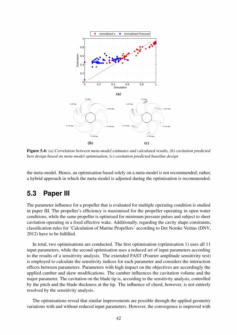
0 0.2 0.4 0.6 0.8 10

0.2

0.4

0.6

0.8

1

Simulation

Est

imat

ion

normalised η normalised Pressure

(a)θ=0 deg.

θ=60 deg.

θ=120 deg.

θ=180 deg.

θ=240 deg.

θ=300 deg.

(b)

θ=0 deg.

θ=60 deg.

θ=120 deg.

θ=180 deg.

θ=240 deg.

θ=300 deg.

(c)

Figure 5.4: (a) Correlation between meta-model estimates and calculated results, (b) cavitation predictedbest design based on meta-model optimisation, (c) cavitation predicted baseline design

the meta-model. Hence, an optimisation based solely on a meta-model is not recommended; rather,a hybrid approach in which the meta-model is adjusted during the optimisation is recommended.

5.3 Paper III

The parameter influence for a propeller that is evaluated for multiple operating condition is studiedin paper III. The propeller’s efficiency is maximised for the propeller operating in open waterconditions, while the same propeller is optimised for minimum pressure pulses and subject to sheetcavitation operating in a fixed effective wake. Additionally, regarding the cavity shape constraints,classification rules for ’Calculation of Marine Propellers’ according to Det Norske Veritas (DNV,2012) have to be fulfilled.

In total, two optimisations are conducted. The first optimisation (optimisation 1) uses all 11input parameters, while the second optimisation uses a reduced set of input parameters accordingto the results of a sensitivity analysis. The extended FAST (Fourier amplitude sensitivity test)is employed to calculate the sensitivity indices for each parameter and considers the interactioneffects between parameters. Parameters with high impact on the objectives are accordingly theapplied camber and skew modifications. The camber influences the cavitation volume and themajor parameter. The cavitation on the blade tip is, according to the sensitivity analysis, controlledby the pitch and the blade thickness at the tip. The influence of chord, however, is not entirelyresolved by the sensitivity analysis.

The optimisations reveal that similar improvements are possible through the applied geometryvariations with and without reduced input parameters. However, the convergence is improved with

42

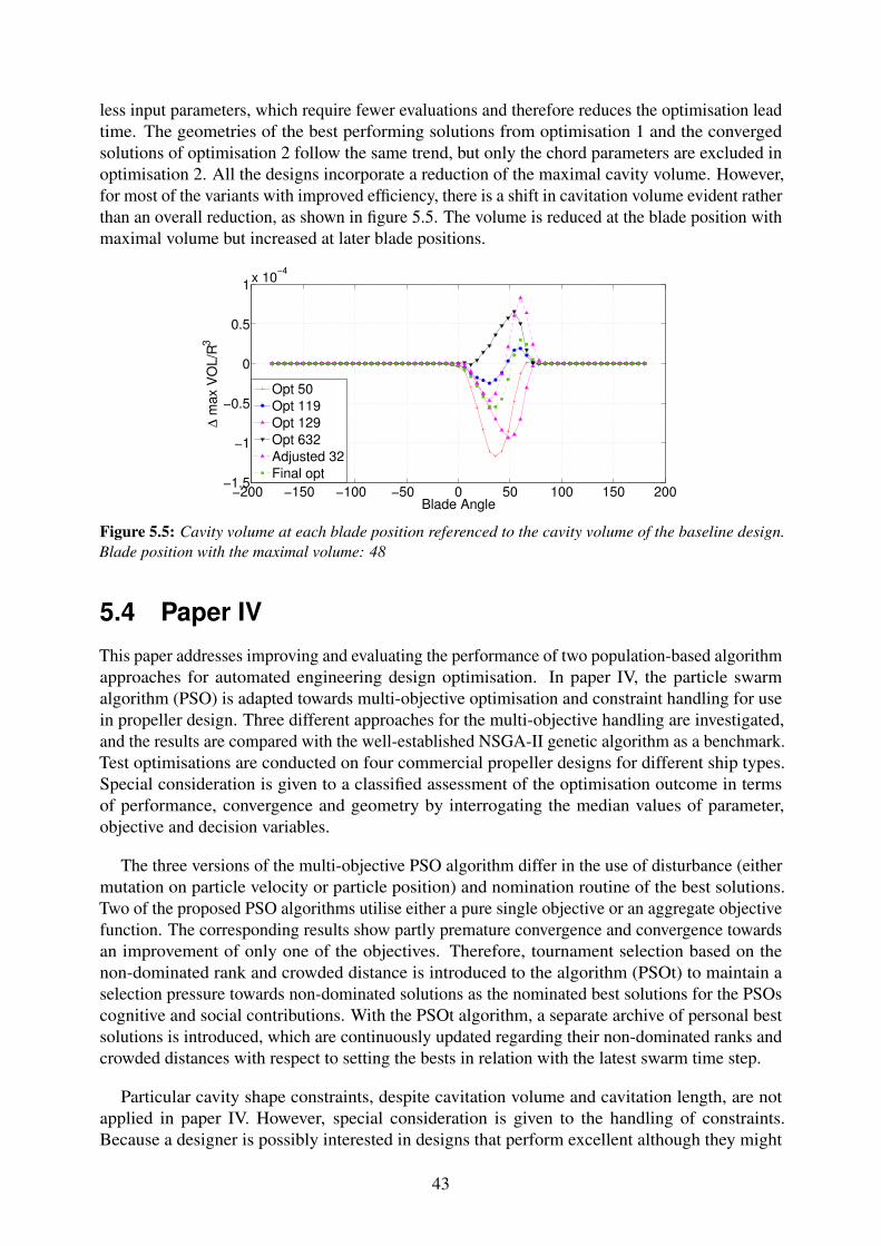
less input parameters, which require fewer evaluations and therefore reduces the optimisation leadtime. The geometries of the best performing solutions from optimisation 1 and the convergedsolutions of optimisation 2 follow the same trend, but only the chord parameters are excluded inoptimisation 2. All the designs incorporate a reduction of the maximal cavity volume. However,for most of the variants with improved efficiency, there is a shift in cavitation volume evident ratherthan an overall reduction, as shown in figure 5.5. The volume is reduced at the blade position withmaximal volume but increased at later blade positions.

−200 −150 −100 −50 0 50 100 150 200−1.5

−1

−0.5

0

0.5

1x 10

−4

Blade Angle

∆ m

ax V

OL

/R3

Opt 50

Opt 119

Opt 129

Opt 632

Adjusted 32

Final opt

Figure 5.5: Cavity volume at each blade position referenced to the cavity volume of the baseline design.Blade position with the maximal volume: 48

5.4 Paper IV

This paper addresses improving and evaluating the performance of two population-based algorithmapproaches for automated engineering design optimisation. In paper IV, the particle swarmalgorithm (PSO) is adapted towards multi-objective optimisation and constraint handling for usein propeller design. Three different approaches for the multi-objective handling are investigated,and the results are compared with the well-established NSGA-II genetic algorithm as a benchmark.Test optimisations are conducted on four commercial propeller designs for different ship types.Special consideration is given to a classified assessment of the optimisation outcome in termsof performance, convergence and geometry by interrogating the median values of parameter,objective and decision variables.

The three versions of the multi-objective PSO algorithm differ in the use of disturbance (eithermutation on particle velocity or particle position) and nomination routine of the best solutions.Two of the proposed PSO algorithms utilise either a pure single objective or an aggregate objectivefunction. The corresponding results show partly premature convergence and convergence towardsan improvement of only one of the objectives. Therefore, tournament selection based on thenon-dominated rank and crowded distance is introduced to the algorithm (PSOt) to maintain aselection pressure towards non-dominated solutions as the nominated best solutions for the PSOscognitive and social contributions. With the PSOt algorithm, a separate archive of personal bestsolutions is introduced, which are continuously updated regarding their non-dominated ranks andcrowded distances with respect to setting the bests in relation with the latest swarm time step.

Particular cavity shape constraints, despite cavitation volume and cavitation length, are notapplied in paper IV. However, special consideration is given to the handling of constraints.Because a designer is possibly interested in designs that perform excellent although they might

43

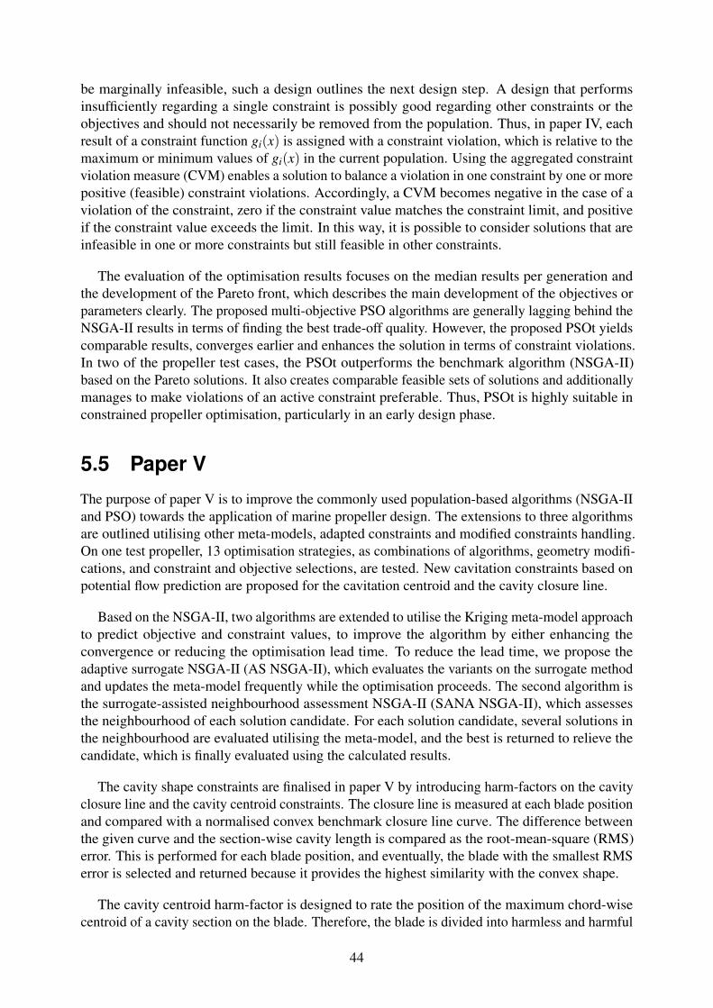
be marginally infeasible, such a design outlines the next design step. A design that performsinsufficiently regarding a single constraint is possibly good regarding other constraints or theobjectives and should not necessarily be removed from the population. Thus, in paper IV, eachresult of a constraint function gi(x) is assigned with a constraint violation, which is relative to themaximum or minimum values of gi(x) in the current population. Using the aggregated constraintviolation measure (CVM) enables a solution to balance a violation in one constraint by one or morepositive (feasible) constraint violations. Accordingly, a CVM becomes negative in the case of aviolation of the constraint, zero if the constraint value matches the constraint limit, and positiveif the constraint value exceeds the limit. In this way, it is possible to consider solutions that areinfeasible in one or more constraints but still feasible in other constraints.

The evaluation of the optimisation results focuses on the median results per generation andthe development of the Pareto front, which describes the main development of the objectives orparameters clearly. The proposed multi-objective PSO algorithms are generally lagging behind theNSGA-II results in terms of finding the best trade-off quality. However, the proposed PSOt yieldscomparable results, converges earlier and enhances the solution in terms of constraint violations.In two of the propeller test cases, the PSOt outperforms the benchmark algorithm (NSGA-II)based on the Pareto solutions. It also creates comparable feasible sets of solutions and additionallymanages to make violations of an active constraint preferable. Thus, PSOt is highly suitable inconstrained propeller optimisation, particularly in an early design phase.

5.5 Paper V

The purpose of paper V is to improve the commonly used population-based algorithms (NSGA-IIand PSO) towards the application of marine propeller design. The extensions to three algorithmsare outlined utilising other meta-models, adapted constraints and modified constraints handling.On one test propeller, 13 optimisation strategies, as combinations of algorithms, geometry modifi-cations, and constraint and objective selections, are tested. New cavitation constraints based onpotential flow prediction are proposed for the cavitation centroid and the cavity closure line.

Based on the NSGA-II, two algorithms are extended to utilise the Kriging meta-model approachto predict objective and constraint values, to improve the algorithm by either enhancing theconvergence or reducing the optimisation lead time. To reduce the lead time, we propose theadaptive surrogate NSGA-II (AS NSGA-II), which evaluates the variants on the surrogate methodand updates the meta-model frequently while the optimisation proceeds. The second algorithm isthe surrogate-assisted neighbourhood assessment NSGA-II (SANA NSGA-II), which assessesthe neighbourhood of each solution candidate. For each solution candidate, several solutions inthe neighbourhood are evaluated utilising the meta-model, and the best is returned to relieve thecandidate, which is finally evaluated using the calculated results.

The cavity shape constraints are finalised in paper V by introducing harm-factors on the cavityclosure line and the cavity centroid constraints. The closure line is measured at each blade positionand compared with a normalised convex benchmark closure line curve. The difference betweenthe given curve and the section-wise cavity length is compared as the root-mean-square (RMS)error. This is performed for each blade position, and eventually, the blade with the smallest RMSerror is selected and returned because it provides the highest similarity with the convex shape.

The cavity centroid harm-factor is designed to rate the position of the maximum chord-wisecentroid of a cavity section on the blade. Therefore, the blade is divided into harmless and harmful

44

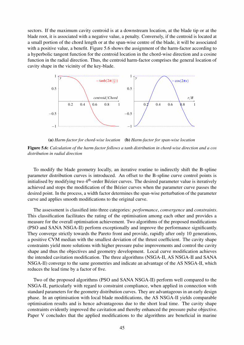
sectors. If the maximum cavity centroid is at a downstream location, at the blade tip or at theblade root, it is associated with a negative value, a penalty. Conversely, if the centroid is located ata small portion of the chord length or at the span-wise centre of the blade, it will be associatedwith a positive value, a benefit. Figure 5.6 shows the assignment of the harm-factor according toa hyperbolic tangent function for the centroid location in the chord-wise direction and a cosinefunction in the radial direction. Thus, the centroid harm-factor comprises the general location ofcavity shape in the vicinity of the key-blade.

− tanh(2π( x2))

0.2 0.4 0.6 0.8 1

−1

−0.5

0.5

1

centroid/Chord

y

(a) Harm-factor for chord-wise location

−cos(2πx)

0.2 0.4 0.6 0.8 1

−1

−0.5

0.5

1

r/R

y

(b) Harm-factor for span-wise location

Figure 5.6: Calculation of the harm-factor follows a tanh distribution in chord-wise direction and a cosdistribution in radial direction

To modify the blade geometry locally, an iterative routine to indirectly shift the B-splineparameter distribution curves is introduced. An offset to the B-spline curve control points isinitialised by modifying two 4th-order Bezier curves. The desired parameter value is iterativelyachieved and stops the modification of the Bezier curves when the parameter curve passes thedesired point. In the process, a width factor determines the span-wise perturbation of the parametercurve and applies smooth modifications to the original curve.

The assessment is classified into three categories: performance, convergence and constraints.This classification facilitates the rating of the optimisation among each other and provides ameasure for the overall optimisation achievement. Two algorithms of the proposed modifications(PSO and SANA NSGA-II) perform exceptionally and improve the performance significantly.They converge strictly towards the Pareto front and provide, rapidly after only 10 generations,a positive CVM median with the smallest deviation of the thrust coefficient. The cavity shapeconstraints yield more solutions with higher pressure pulse improvements and control the cavityshape and thus the objectives and geometry development. Local curve modification achievesthe intended cavitation modification. The three algorithms (NSGA-II, AS NSGA-II and SANANSGA-II) converge to the same geometries and indicate an advantage of the AS NSGA-II, whichreduces the lead time by a factor of five.

Two of the proposed algorithms (PSO and SANA NSGA-II) perform well compared to theNSGA-II, particularly with regard to constraint compliance, when applied in connection withstandard parameters for the geometry distribution curves. They are advantageous in an early designphase. In an optimisation with local blade modifications, the AS NSGA-II yields comparableoptimisation results and is hence advantageous due to the short lead time. The cavity shapeconstraints evidently improved the cavitation and thereby enhanced the pressure pulse objective.Paper V concludes that the applied modifications to the algorithms are beneficial in marine

45

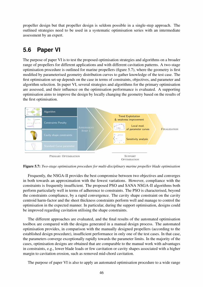
propeller design but that propeller design is seldom possible in a single-step approach. Theoutlined strategies need to be used in a systematic optimisation series with an intermediateassessment by an expert.

5.6 Paper VI

The purpose of paper VI is to test the proposed optimisation strategies and algorithms on a broaderrange of propellers for different applications and with different cavitation patterns. A two-stageoptimisation procedure is outlined for marine propellers (figure 5.7), where the geometry is firstmodified by parameterised geometry distribution curves to gather knowledge of the test case. Thefirst optimisation set-up depends on the case in terms of constraints, objectives, and parameter andalgorithm selection. In paper VI, several strategies and algorithms for the primary optimisationare assessed, and their influence on the optimisation performance is evaluated. A supportingoptimisation aims to improve the design by locally changing the geometry based on the results ofthe first optimisation.

AlgorithmPopulation

Initialisation

Termination

Parents

Offspring

Recombination

Mutation

Survivorselection

Parentsselection

Constraints Penalty

KT

CAVV olumeCAVShape

−1.5 −1 −0.5 0.5 1 1.5

−1

1

x

y

Cavity shape constraints

Standard Curve parameter

Skew Angle

AssessmentStep 1

Trend Exploitation& weakness improvement

Local mod.of parameter curvesr/R

0.3 0.4 0.5 0.6 0.7 0.8 0.9 1

C(r

)/D

BaselineNew Design

Pt

Sensitivity analysis

Finalization

SupportOptimisation

Primary Optimisation

Figure 5.7: Two-stage optimisation procedure for multi-disciplinary marine propeller blade optimisation

Frequently, the NSGA-II provides the best compromise between two objectives and convergesin both towards an approximation with the fewest variations. However, compliance with theconstraints is frequently insufficient. The proposed PSO and SANA NSGA-II algorithms bothperform particularly well in terms of adherence to constraints. The PSO is characterised, beyondthe constraints compliance, by a rapid convergence. The cavity shape constraint on the cavitycentroid harm-factor and the sheet thickness constraints perform well and manage to control theoptimisation in the expected manner. In particular, during the support optimisation, designs couldbe improved regarding cavitation utilising the shape constraints.

The different approaches are evaluated, and the final results of the automated optimisationtoolbox are compared with the designs generated in a manual design process. The automatedoptimisation provides, in comparison with the manually designed propellers (according to theestablished design procedure), insufficient performance in only one of the test cases. In that case,the parameters converge exceptionally rapidly towards the parameter limits. In the majority of thecases, optimisation designs are obtained that are comparable to the manual work with advantagesin constraints, e.g., lower blade loads or few cavitation or cavity shapes associated with a highermargin to cavitation erosion, such as removed mid-chord cavitation.

The purpose of paper VI is also to apply an automated optimisation procedure to a wide range

46

of test propellers and evaluate the optimal results to determine propeller-dependent optimisationsettings. The optimised propellers are, with respect to the applied settings, reasonably good;the designer may, however, consider design limitations that are beyond the applied evaluationmethods. However, the generated designs guide the designer to find better solutions faster. Todetermine reliable guidelines for optimisation settings, further optimisations need to be assessedand categorised according to the propeller design demands, e.g., a focus on cavitation, propellerefficiency or pressure pulse. In that context, the optimisation routine can be improved regardingstricter consideration of the KT constraint and in complexity, e.g., considering several operatingconditions or interchangeable settings of the objectives and constraints can be beneficial to achievebetter and possibly novel designs faster.

47

An expert is a person who has made all themistakes that can be made in a very narrowfield.

Niels Bohr

6 Discussion

The aim of this thesis is to further improve the procedure of propeller design by supplementing thepropeller designer with automated optimisation. The approach should assist the designer in findingbetter designs faster while simultaneously enhancing multi-disciplinary evaluation to reduce thelead time for propeller development and increase the quality of a design. Two tracks are thereforeexamined, namely, the strategies for optimisation and the improvement of constraints, and bothare aligned with the manual design procedure.

In the previous chapter 5, the performed work was outlined and the results of each study werediscussed separately. This chapter aims to provide a holistic perspective and show how the researchis connected.

In the papers attached to this thesis, the complexity of optimisation is consistently increasedto take the optimisation procedure to the same level of design considerations as done by anexperienced designer. In this manner, the optimisation outcome becomes more competitive withthe manual design and thus more useful for the designer to find new designs faster and with lessuser interaction.

The work performed for this thesis continuous thematically where Han (2008) finished withthe optimisation of propeller blade geometry in interaction with the ship hull and the rudder, butwith consideration of sheet cavitation as a design constraint. This set-up is the desired approach inpropeller design because of the interaction effects between the propeller and its inflow, as wellas a direct coupling to the hull geometry. Ideally, the propeller designer has the responsibilityof designing the entire propulsion unit, including the hull lines of the aft ship to take interactioneffects into account (Grunditz, 2015). Han (2008) also recommends including optimisation ofthe rudder geometry. However, simultaneously optimising hull lines and the propeller bladegeometry enlarges the design space considerably and accordingly requires more evaluations ofdesign alternatives. Numerical effort typically hinders such optimisation. In this thesis, thecomputational effort of such optimisation with hull interactions is addressed in a set-up of thenumerical simulations that consistently considers the computational effort by reducing the meshsize (with consideration of the accuracy) to a zonal approach, computing the propeller performancein a hybrid-RANS approach and re-using the converged simulations of the baseline design for thecomputation of a new variant. However, the numerical effort is considerable and hardly compatiblewith automated optimisation in a daily routine.

Optimisation algorithms require a certain number of objective function evaluations to gather

49

knowledge of the problem definition before they can converge to ’the optimal’ solution. Through-out this thesis, optimisations are entirely based on population-based optimisation algorithms. Thishas several reasons: population-based algorithms are to the greatest extent independent from thestarting point of the optimisation and are able to find the global optimum, they are independentfrom continuity of objective functions and objectives, and they are, unlike e.g. adjoint methods,readily applicable in unsteady flow simulations and generally very robust. However, the algorithmsrequire a large number of evaluations, which increase with the number of design variables andconstraints.

The lack of convergence is particularly evident from the optimisation performed in paper I,where too many decision variables are applied in combination with a population size that is toosmall. The optimisation is additionally hindered by numerous constraints that are neither alignedwith each other nor with the objective functions. However, the outcome of the optimisationprovides awareness of the effect of the blade geometry on the effective wake and, most importantly,a connection between the predicted cavity shape and the pressure pulse objective, as well as theneed for improved optimisation methods, from which the emphasis of this thesis originates. Inpaper I, the assessment of the optimisation outcome provides a relation between the cavity shapeand the propeller-induced pressure pulses and indicates a minor impact of cavitation volume onthe efficiency. This initiated the first track that is followed throughout this thesis. The cavitationconstraints in paper I are applied according to (Han et al., 2006) and refined in terms of cavityshape evaluation and a broadened range of calculated time steps that are interrogated. Han et al.(2006) examined only the angular blade position with the maximum cavity volume, which isreasonable when only the maximum cavity volume is constrained. However, when certain typesof cavity shapes have a greater effect on the applied objectives, as indicated in paper I and paperVI, a refined evaluation is important.

Throughout this thesis, cavity shape constraints are refined. From the incipient constraints forthe global appearance of cavitation, they evolved to specialised shape constraints with either anexplicit effect on the pressure pulse objective, e.g., the change in cavity volume, or an impliciteffect on the objectives by reducing, for instance, the thickness of the sheet cavity or by controllingthe cavity shape and location on the blade. The latter is also utilised to avoid global cavitation thatis known to possibly result in erosive local cavitation, as discussed in paper V and related to Barket al. (2004) and Foeth (2008). Although they are developed in connection with the prediction of apotential flow simulation prediction, they can readily be transferred to high-fidelity methods.

The evaluation of cavitation constraints for automated optimisation is generally seldom ad-dressed to such a detailed level of cavitation interrogation. In the majority of propeller optimi-sations, only the general cavitation amount is constrained, if at all. Han et al. (2006) utilises thecavitation volume and sectional cavitation area, pressure coefficient and Keller criteria; Kamarloueiet al. (2014) also applies the Keller criteria as well as the Bucket diagram; Gaggero et al. (2009)and Bertetta et al. (2012) use the cavity plan form area. All apply potential methods for predictingthe propeller performance. However, the constraints are rather useful for constraining only thetotal amount of cavitation rather than the location and shape. A restriction on the cavity shaperesults in possible trade-off solutions, which allow for higher propeller efficiency. The majorityof optimal solutions, obtained from optimisation throughout this thesis, provide a reduction incavity volume, which is related to the consequent restriction of cavity constraints, relative to thecorresponding baseline design.

It is crucial for automated optimisation to present information regarding a design solution in

50

single values. Gaggero et al. (2009) and Bertetta et al. (2012) apply cavitation as a constraint inpropeller efficiency and propeller noise optimisation by averaging different working conditionsrelated to a statistical analysis of the wake field, thereby reducing the information obtained from theflow simulations to a single averaged value. This is adequate for the applied cavitation constrainton the cavity plan form area. However, the aim of an intricate analysis of the sheet cavity formationrequires a finer interrogation of the prediction, which is accomplished by the conservative approachof determining the blade position with the maximum cavity volume (key-blade) and includingthe significant blade positions in the vicinity of the key-blade, from which the worst cavity shapeconstraint is selected.

Evidently, the cavity shape improves with the assistance of the proposed cavity shape constraints.However, the optimal trade-off propeller in paper III frequently provides results that shifted thecavitation towards blade positions that are not assessed during the optimisation. Such behaviouris similarly obtained from the optimal solution of Opt-1 6.1c and the optimal result from paperI (figure 6.1a). The manual design of Opt-1 also yields, however, a shifted cavitation volumetowards later blade positions. Such behaviour is certainly beneficial for the pressure pulseobjective but can still lead to erosive cavitation outside the interrogated blade positions. This isparticularly obvious from Opt-4 6.1f, where only the assessed blade positions achieve a reductionin cavitation volume, although the cavity volume is notably small. Figure 6.1 presents thenormalised change cavitation volume (∆maxVol/R3), referenced to the baseline design. Thus, ifthe manually designed benchmark or the optimised solution provide ∆maxVol/R3 below zero,there is a reduction in volume. For the majority of the cases optimised throughout this thesis, thecavitation is improved and from the comparison in figure 6.1 typically more restrictive regardingcavity volume compared to the benchmark designs. The optimisation outcome still requires criticalassessment by an experienced designer to avoid the risk of optimised results that are biased by thetools or constraints applied.

Constraints that are adapted to the objectives increase the connection between the optimisationaim and the decision variables, which improves the behaviour of the optimisation algorithm toenhance convergence and thereby reduce the lead time; this is the second track followed throughoutthis thesis. The first paper starts with a detailed analysis of the propeller working in the flow fieldaround the hull and indicates that this interaction is important for ensuring a robust design, but inthe design phase when exploring the design space, it is impractical due to a long evaluation pervariant. Han (2008) already indicated the need for reduced computational time and recommendedresponse surface estimations as a possible remedy.

Consequently, the lead time of propeller optimisation is particularly addressed in paper II, fo-cusing on the ability to substitute computations with estimations by meta-models. The applicationof meta-models in optimisations as well as optimisation in marine applications is not uncommon,e.g., Schmitz et al. (2002), Maisonneuve (2003) or Harries (2010). However, regarding propellerdesign, the reported research abates, and most of the recent research is restricted to hydrodynamicforce predictions, e.g., (Roddy et al., 2008) and (Calcagni et al., 2010); only Koushan (2000)includes the estimation of propeller-induced pressure pulse by an artificial neural network.

The application of meta-models for propeller optimisation including cavitation constraintsis challenging, as indicated by the results from paper II. The performance of meta-models onthe propeller performance, predicted by the potential flow simulation, varies both among themeta-models and the quantity that is estimated. In particular, the cavity shape constraints arehardly captured correctly; only the correct trends could be realised. However, optimisation that

51

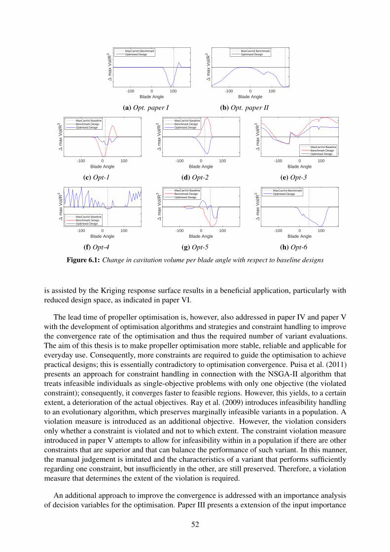
Blade Angle-100 0 100

" m

ax V

ol/R

3

MaxCavVol BenchmarkOptimised Design

(a) Opt. paper I


" m

ax V

ol/R

3


(b) Opt. paper II


" m

ax V

ol/R

3

MaxCavVol BaselineBenchmark DesignOptimised Design

(c) Opt-1


" m

ax V

ol/R

3


(d) Opt-2


" m

ax V

ol/R

3


(e) Opt-3


" m

ax V

ol/R

3


(f) Opt-4


" m

ax V

ol/R

3


(g) Opt-5


" m

ax V

ol/R

3


(h) Opt-6

Figure 6.1: Change in cavitation volume per blade angle with respect to baseline designs

is assisted by the Kriging response surface results in a beneficial application, particularly withreduced design space, as indicated in paper VI.

The lead time of propeller optimisation is, however, also addressed in paper IV and paper Vwith the development of optimisation algorithms and strategies and constraint handling to improvethe convergence rate of the optimisation and thus the required number of variant evaluations.The aim of this thesis is to make propeller optimisation more stable, reliable and applicable foreveryday use. Consequently, more constraints are required to guide the optimisation to achievepractical designs; this is essentially contradictory to optimisation convergence. Puisa et al. (2011)presents an approach for constraint handling in connection with the NSGA-II algorithm thattreats infeasible individuals as single-objective problems with only one objective (the violatedconstraint); consequently, it converges faster to feasible regions. However, this yields, to a certainextent, a deterioration of the actual objectives. Ray et al. (2009) introduces infeasibility handlingto an evolutionary algorithm, which preserves marginally infeasible variants in a population. Aviolation measure is introduced as an additional objective. However, the violation considersonly whether a constraint is violated and not to which extent. The constraint violation measureintroduced in paper V attempts to allow for infeasibility within in a population if there are otherconstraints that are superior and that can balance the performance of such variant. In this manner,the manual judgement is imitated and the characteristics of a variant that performs sufficientlyregarding one constraint, but insufficiently in the other, are still preserved. Therefore, a violationmeasure that determines the extent of the violation is required.

An additional approach to improve the convergence is addressed with an importance analysisof decision variables for the optimisation. Paper III presents a extension of the input importance

52

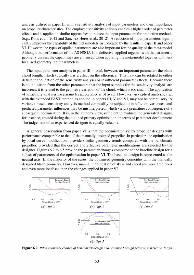
analysis utilised in paper II, with a sensitivity analysis of input parameters and their importanceon propeller characteristics. The employed sensitivity analysis enables a higher order of parametereffects and is applied in similar approaches to reduce the input parameters for prediction methods(e.g., Roos et al., 2012 and Sanchez-Heres et al., 2012). A reduction of input parameters signifi-cantly improves the capability of the meta-models, as indicated by the results in paper II and paperVI. However, the types of applied parameters are also important for the quality of the meta-model.Although the performance of the AS NSGA-II is defective, applied together with the parametricgeometry curves, the capabilities are enhanced when applying the meta-model together with lesslocalised geometry input parameters.

The input parameter analysis in paper III missed, however, an important parameter: the bladechord length, which typically has a effect on the efficiency. This flaw can be related to eitherdeficient application of the sensitivity analysis or insufficient parameter effects. Because thereis no indication from the other parameters that the input samples for the sensitivity analysis areincorrect, it is related to the geometry variation of the chord, which is too small. The applicationof sensitivity analysis for parameter importance is of avail. However, an explicit analysis, e.g.,with the extended FAST method as applied in papers III, V and VI, may not be compulsory. Avariance-based sensitivity analysis method can readily be subject to insufficient variances, andpredicted parameter influences may be misinterpreted, which yield a premature convergence of asubsequent optimisation. It is, in the author’s view, sufficient to evaluate the generated designs,for instance, created during the outlined primary optimisation, in terms of parameter development.The judgement of an experienced designer is equally valuable.

A general observation from paper VI is that the optimisation yields propeller designs withperformance comparable to that of the manually designed propeller. In particular, the optimisationby local curve modifications provide similar geometry trends compared with the benchmarkpropeller, provided that the correct and effective parameter modifications are selected by thedesigner. Figures 6.2 to 6.5 provide the parameter changes compared to the baseline design for asubset of parameters of the optimisation in paper VI. The baseline design is represented as theneutral axis. In the majority of the cases, the optimised geometry coincides with the manuallydesigned blade geometry. However, manual modification of skew and chord are more ambitiousand even more localised than the changes applied in paper VI.

Blade Radius [r/R]0.2 0.4 0.6 0.8 1

" P

/D

Benchmark DesignOptimised Design

(a) Opt-2Blade Radius [r/R]

0.4 0.6 0.8 1

" P

/D


(b) Opt-3Blade Radius [r/R]

0.4 0.6 0.8 1

" P

/D


(c) Opt-4

Blade Radius [r/R]0.4 0.6 0.8 1

" P

/D Benchmark DesignOptimised Design

(d) Opt-5

Figure 6.2: Pitch geometry change of benchmark design and optimised design relative to baseline design

53

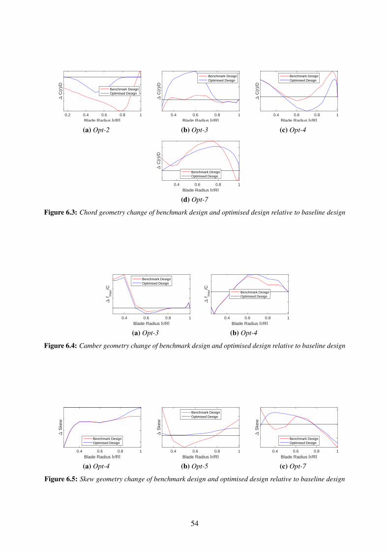
Blade Radius [r/R]0.2 0.4 0.6 0.8 1

" C

(r)/

D



0.4 0.6 0.8 1

" C

(r)/

D



0.4 0.6 0.8 1

" C

(r)/

D


(c) Opt-4


" C

(r)/

D


(d) Opt-7

Figure 6.3: Chord geometry change of benchmark design and optimised design relative to baseline design


" f m

ax/C



0.4 0.6 0.8 1

" f m

ax/C


(b) Opt-4

Figure 6.4: Camber geometry change of benchmark design and optimised design relative to baseline design


" S

kew



0.4 0.6 0.8 1

" S

kew



0.4 0.6 0.8 1

" S

kew


(c) Opt-7

Figure 6.5: Skew geometry change of benchmark design and optimised design relative to baseline design

54

It is not knowledge, but the act of learning,not possession but the act of getting there,which grants the greatest enjoyment.

Carl Friedrich Gauss

7 Conclusion

Propeller design is fascinating. In principle, propellers appear to be interchangeable; the generaldesign has not changed in approximately 100 years. However, each design is unique, and the flowaround the propeller blades is remarkably complex, which requires attention in the design of apropulsion unit. The goal of this thesis conforms to this attention by improving the procedure ofpropeller design through automated optimisation as a supplementary tool to assist the designer infinding better designs faster.

Two tracks are followed to improve automated propeller design: i) the development of strategiesand concepts for propeller optimisation, with the objective of developing optimisation algorithmswith enhanced convergence and consideration of constraints, and ii) the extension and explorationof constraints that are adapted to the principles and design considerations of the manual designprocedure. The work performed on the two tracks contributes to further developing population-based optimisation algorithms and constraints that automatically judge the cavitation on thepropeller. Additional constraints and limitations are added to the optimisation procedure, whichare often neglected in study cases but that commonly have to be considered by the designers. Thealgorithms and constraints are implemented in the designer’s toolbox for computer-aided propellerdesign and can be used on an everyday design task with access to all analysis tools available to thedesigner.

The optimisation procedure handles multi-disciplinary evaluation of multiple objectives andconstraints without user interaction; still, it yields propeller designs that are comparable witha manually designed propeller. The developed algorithms are persuasive in their ability tohandle constraints, which relates to a memory effect from storing the best solutions in the PSOand a continuous evaluation of the neighbourhood in the SANA NSGA-II. Both algorithmsare advantageous in the applied cases compared to the NSGA-II. The AS NSGA-II provides atremendous benefit in lead time while achieving the same results as the NSGA-II when appliedwith local curve modification. To determine reliable guidelines for optimisation settings, furtheroptimisations need to be assessed and categorised according to the propeller design demands, e.g.,a focus on cavitation, propeller efficiency or pressure pulse. However, the proposed preliminaryand supportive optimisation is one step in that direction and enhances the expectation of trulyfinding an optimal design.

Cavitation constraints clearly improve the quality of the optimisation outcome and the con-vergence of the optimisation by enhancement of the objective. The pressure pulse objective is

55

evidently related to certain types of cavitation and frequently provides in the conducted optimisa-tion the largest possible gains, which is related to the focus on cavitation constraints. Thus, incases with a clear focus on the efficiency, it may be beneficial to consider the pressure pulse as aconstraint rather than an objective.

The manual design is superior in terms of design quality, but automated optimisation possessesthe advantage of a broader exploration of the design space at the same lead time. There is, however,no evidence that optimisation guarantees better results. Optimisation, manual or automated, issubject to applied limitations provided by, e.g., analysis tools. The manual design is advantageousbecause the designer may consider limitations that are not provided by any analysis tools. It isstill the designer’s responsibility to set up a suitable combination of objectives, constraints anddecision variables to achieve a successful optimisation. With an improved and faster algorithm,the designer could be able to proceed towards the next design cycle in a shorter amount of time.

56

The more I learn, the more I realize howmuch I don’t know.

Albert Einstein

8 Further Work

The development of innovative optimisation algorithms and strategies suited for propeller designoptimisation will not end here. Automated optimisation for practical applications is just emerging.The general question is what to prioritise: the accuracy or the usability. Computational methods ofhigher fidelity analysis are typically more accurate and provide more details on the flow around thepropeller blade because they comprise more physical reality than potential methods. However, thepractical application of optimisation methods requires the consideration of numerous limitations,which can easily be extended from those realised within this thesis. Consequently, the mostobvious improvement can be realised with variable fidelity optimisation, composed of RANSsimulations, potential flow simulations and meta-models, together with an algorithm that is able todecide which evaluation to utilise. However, the optimisation with consideration of the hull is stilltoo demanding in the general blade geometry finding phase.

Further work, despite the fidelity of numerical evaluation methods, can be categorised intooptimisation and propeller design, constraints development and optimisation guidance.

Optimisation and propeller designThe optimisation algorithms should be further developed to automatically resolve when to analysethe propeller with simulations and when meta-model estimations are sufficient. The decision willthus depend on both the current training status of the meta-model and the distance of the parameterlocation in the design space relative to other computed solutions. Such a decision routine canreadily be extended to several levels of variable fidelity, but with careful consideration of matchingconstraints and objective representation of the different analysis tools.

Automated optimisation has the potential to become superior to manual design. The presentedoptimisation outlines a routine that imitates the manual design process to assist the designer.However, the optimisation can readily be extended to additionally consider several off-designconditions simultaneously and thereby enhance the product quality by adaptation to the entire lifecycle of the propeller and not only a single design point. In the case of a CPP, this will includean underlying optimisation of the optimal blade pitch adjustment for the off-design conditions.Manual design is of course capable of such optimisation; however, lead time typically restrictssuch extensive investigations.

Introducing several conditions to the optimisation can also be used for optimisation in a semi-unsteady wake, e.g., to account for the changing inflow to the propeller in waves. In such ascenario, the efficiency could be considered as an aggregated function, while the constraints aresubject to the most deficient performance.

57

ConstraintsAutomated optimisation depends more on the specified limitations and capabilities of the appliedanalysis tools than manual design. Several considerations of the designer during the manual designprocess can be considered by the parameter limits, e.g., maximum rake to avoid interference withthe hull or pod. However, there are important design considerations that have to be consideredduring the optimisation by simulations, e.g., tip vortex inception. Consequently, the continuousdevelopment of analysis tools is part of future work for propeller optimisation to further improvepossible constraints. Hence, we are improving a semi-analytical method for tip vortex inceptionbased on the simulations of a vortex lattice potential flow simulation. New cavitation constraintsare also under development for indicating erosive cavitation by evaluation of the cavitationcollapse.

However, the proposed constraints on cavitation could also be improved to be more flexibleand adaptable to the cavitation on the baseline design. Particularly, the cavitation closure lineharm-factor performed disappointingly due to lacking similarity between the specified polynomialand the simulated cavitation shape. This will be cured by fitting the polynomial to the cavity shapeof the baseline. However, other potential methods that are able to indicate the re-entrant jet areinteresting to be included in the optimisation and constraints development.

Optimisation guidanceEventually, the strategies for automated propeller optimisation will become more diverse yetuseful in particular problems. Hence, it is recommended to establish a database for optimisationproblems with respect to propeller design demands, e.g., a focus on cavitation, propeller efficiencyor pressure pulse. This should lead to the determination of reliable guidelines for optimisationsettings.

58

References

Abdel-Maksoud, M., ed. (2011). Proceedings of the Second International Symposium on MarinePropulsors. (Hamburg, Germany). Hamburg University of Technology.

Andersen, P., A.-S. Borrod, and H. Blanchot (2005). Evaluation of the service performance ofships. Marine Technology 42.4, 177–183.

Backlund, P. B., D. Shahan, and C. C. Seepersad (2010). Metamodeling techniques for multidi-mensional ship design problems. Ship Science & Technology 4.7, 43–54.

Bark, G., N. Berchiche, and M. Grekula (2004). Application of principles for observation andanalysis of eroding cavitation - The EROCAV observation handbook. Report. Dept. of NavalArchitecture and Ocean Engineering.

Benini, E. (2003). Multiobjective design optimization of B-screw series propellers using evolu-tionary algorithms. Marine Technology 40.4, 229–238.

Berger, S. et al. (2014). A Two-Stage Optimisation Method for Full-Scale Marine PropellersWorking Behind a Ship. Ship Technology Research 61.2, 64–79.

Bertetta, D. et al. (2012). CPP propeller cavitation and noise optimization at different pitches withpanel code and validation by cavitation tunnel measurements. Ocean Engineering 53, 177–195.

Bertram, V. (2012). Practical ship hydrodynamics. Elsevier.Binns, J., R. Brown, and N. Bose, eds. (2013). Proceedings of the Third International Symposium

on Marine Propulsors. (Launceston, Tasmania, Australia). University of Tasmania.Blount, D. (1993). “Prospects for Hard Chine, Monohull Vessels”. Proceedings: FAST’93.Box, G. E. and K. Wilson (1951). On the experimental attainment of optimum conditions. Journal

of the Royal Statistical Society. Series B (Methodological) 13.1, 1–45.Breslin, J. P. et al. (1982). Theoretical and experimental propeller-induced hull pressures arising

from intermittent blade cavitation, loading, and thickness. Transactions-Society of NavalArchitects and Marine Engineers 90, 111–151.

Burnside, O. H., D. D. Kana, and F. E. Reed (1979). A design procedure for minimizing propellerinduced vibration in hull structural elements. Export Date: 17 July 2012 Source: Scopus.

Calcagni, D. et al. (2010). “Automated Marine Propeller Design Combining HydrodynamicsModels and Neural Networks”. First International Symposium on Fishing Vessel EnergyEfficiency E-Fishing.

Carlton, J. (2007). “22 - Propeller design”. Marine Propellers and Propulsion (Second Edition).Ed. by J. Carlton. Second Edition. Oxford: Butterworth-Heinemann, pp. 435 –463.

Chandrashekarappa, P. and R. Duvigneau (2007). Radial basis functions and kriging metamodelsfor aerodynamic optimization. Tech. rep. 6151. Unite de recherche INRIA Sophia Antipolis.

Costa, J., L. Pronzato, and E. Thierry (1999). “A comparison between Kriging and radial basisfunction networks for nonlinear prediction.” NSIP, 726–730.

Cummings, D. E. (1973). Numerical Prediction of Propeller Characteristics. Journal of ShipResearch 17.1. cited By 0, 12–18.

Deb, K. and R. B. Agrawal (1995). Simulated Binary Crossover for Continuous Search Space.Complex Systems 9, 115–148.

Deb, K. and M. Goyal (1996). A Combined Genetic Adaptive Search (GenaAS) for EngineeringDesign. Computer Science and Informatics 26, 30–45.

Deb, K. et al. (2002). A Fast Elitist Multi-Objective Genetic Algorithm: NSGA-II. IEEE Transac-tions on Evolutionary Computation 6, 182–197.

DNV (2010). Rules for Classification of Ships. Det Norske Veritas.– (2012). Calcualtion of Marine Propellers. Det Norske Veritas.

59

Ellbrant, L. (2014). Multi-objective CFD-based design method for axial compressors. ChalmersUniversity of Technology.

Fine, N. E. (1992). “Nonlinear Analysis of Cavitating Propellers in Nonuniform Flow”. PhD thesis.Massachusetts Institute of Technology.

Foeth, E.-J. (2008). “The structure of three-dimensional sheet cavitation”. PhD Thesis. UniversityDelft.

– (2015). “Propeller optimization using an unsteady Boundary-Element Method”. Fourth Inter-national Symposium on Marine Propulsors. Ed. by S. A. Kinnas. Vol. II. The University ofTexas at Austin, 27–32.

Froude, R. (1889). On the part played in propulsion by differences of fluid pressure. Transactionsof the Institute of Naval Architects 30, 390–405.

Gaggero, S and S Brizzolara (2009). “Parametric CFD optimization of fast marine propellers”.10th International Conference on Fast Sea Transportation, Athens, Greece.

Goldstein, S. (1929). On the Vortex Theory of Screw Propellers. Proceedings of the Royal Societyof London A: Mathematical, Physical and Engineering Sciences 123.792, 440–465.

Greeley, D. S. and J. E. Kerwin (1982). Numerical methods for propeller design and analysis insteady flow. Transactions-Society of Naval Architects and Marine Engineers 90, 415–453.

Griffin, P (1998). “Computational techniques for the design and analysis of cavitating propellerblades”. Master’s thesis.

Griffin, P. E. and S. A. Kinnas (1998). A Design Method for High-Speed Propulsor Blades. Journalof Fluids Engineering 120.3, 556–562.

Grunditz, G. (2015). Optimizinf Propeller and Propulsion. Marine Technology 52.1, 48–55.Han, K.-J. (2008). Numerical optimization of hull/propeller/rudder configurations. [Doktorsavhan-

dlingar vid Chalmers tekniska hogskola]. Ny serie, Goteborg: Chalmers University of Technol-ogy, xii, 88 s.

Han, K.-J., G. Bark, and B. Regnstrom (2006). A Procedure for Optimizing Cavitating PropellerBlades in a Given Wake. Ship Technology Research 53.1, 39–52.

Harries, S. (2010). “Investigating Multi-dimensional Design Spaces Using First Principle Meth-ods”. Seventh International Conference On High-Performance Marine Vehicles (HIPER).

He, L (2010). “Numerical simulation of unsteady rotor/stator interaction and application topropeller/rudder combination (UT-OE Report 10-05)”. PhD thesis. University of Texas atAustin, Dept. of Civil Engineering.

He, L., S. Chang, and S. Kinnas (2010). MPUF-3A Version 3.0. Report. University of Texas.He, L., Y. Tian, and S. Kinnas (2011). MPUF-3A Version 3.1. Report. University of Texas.Hildebrand, J. A. (2009). Anthropogenic and natural sources of ambient noise in the ocean. Marine

Ecology Progress Series 395, 5–20.ISSC, ed. (2006). Dynamic Response. Vol. 1. 16th International Ship and Offshore Structures

Congress.ITTC (1999). ITTC – Recommended Procedures; Performance, Propulsion 1978 ITTC Perfor-

mance Prediction Method. International Towing Tank Conference.– (2002). “The Specialist Committee on Speed and Powering Trails”. 2. ITTC. 23rd International

Towing Tank Conference.– (2008). ITTC – Recommended Procedures and Guidelines; Testing and Extrapolation Methods,

Propulsion, Performance, Predicting Powering Margins. International Towing Tank Conference.Janson, C and L Larsson (1996). “A method for the optimization of ship hulls from a resistance

point of view”. 21st Symposium on Naval Hydrodynamics, Trondheim, Norway.Kamarlouei, M. et al. (2014). Multi-objective evolutionary optimization technique applied to

propeller design. Acta Polytechnica Hungarica 11.9, 163–182.

60

Kerwin, J, S Kinnas, and M. Wilson (1986). “Experimental and analytical techniques for the studyof unsteady propeller sheet cavitation”. Symposium on Naval Hydrodynamics, 16th. Ed. byW. C. Webster. Office of Naval Research, National Academy Press, 387–414.

Kerwin, J. E. (1961). “The solution of propeller lifting surface problems by vortex lattice methods”.PhD thesis. DTIC Document.

Kerwin, J. E. and J. B. Hadler (2010). Principles of Naval Architecture Series: Propulsion. TheSociety of Naval Architects and Marine Engineers (SNAME).

Kinnas, S. and N. Fine (1989). “Theoretical prediction of midchord and face unsteady propellersheet cavitation”. International Conference on Numerical Ship Hydrodynamics, 5th.

Kinnas, S. A. (1985). “Non-Linear Corrections to the Linear Theory for the Prediction of theCavitating Flow Around Hydrofoils.” PhD thesis. Massachusetts Institute of Technology.

Kinnas, S. A. (1991). Leading-edge corrections to the linear theory of partially caviting hydrofoils.Journal of Ship Research 35.1, 15–27.

– (1996). An international consortium on high-speed propulsion. Marine Technology and SNAMENews 33, 203–210.

Kinnas, S. A. and N. E. Fine (1993a). A numerical nonlinear analysis of the flow around two-andthree-dimensional partially cavitating hydrofoils. Journal of Fluid Mechanics 254, 151–181.

– (1993b). A numerical nonlinear analysis of the flow around two-and three-dimensional partiallycavitating hydrofoils. Journal of Fluid Mechanics 254, 151–181.

Koushan, K. (2000). “Prediction of Prepeller Induced Pressure Pulses Using Artificial NeuralNetworks”. 1st International Conference on Computer Application and Information Technologyin Maritime Industries, 248–254.

Kutta, W. (1910). Uber eine mit den Grundlagen des Flugproblems in Beziehung stehendezweidimensionale Stromung. Sitzungsbericht d. Bayr. Akad. d. Wiss., math.-phys. Klasse,Munchen 2, 65.

Lee, C.-S. (1979). “Prediction of steady and unsteady performance of marine propellers with orwithout cavitation by numerical lifting-surface theory”. PhD thesis. Massachusetts institute ofTechnology.

Lee, C.-S. et al. (2010). Performance optimization of marine propellers. International Journal ofNaval Architecture and Ocean Engineering 2.4, 211–216.

Lee, S.-K., M. Liao, and S. Wang (2006). “Propeller-induced hull vibration—analytical methods”.Proceedings of the second international ship noise and vibration conference. London, UK, June.Vol. 28. Citeseer.

Lerbs, H. W. (1952). Moderately loaded propellers with a finite number of blades and an arbitrarydistribution of circulation. Trans. SNAME 60.

Maisonneuve, J.-J. (2003). “Application Examples From Industry”. OPTIMISTIC Optimizationin Marine Design. Ed. by L. Birk and S. Harries. Berlin: Mensch & Buch Verlag. Chap. 7,pp. 151–172.

MAN (2011). Basic Principles of Ship Propulsion.Mishima, S. (1996). “Design of Cavitating Propeller Blades in Non-Uniform Flow by Numerical

Optimization”. PhD Thesis. Massachusetts Institute of Technology.Munk, M. M. (1919). Isoperimetrische Aufgaben aus der Theorie des Fluges. Gottingen: Di-

eterichsche Universitats-Buchdruckerei.Olsen, S. A. (2001). “Optimisation of propellers using the vortex-lattice method”. PhD thesis.

Technical University of Denmark.Peri, D. (2009). Self-Learning Metamodels for Optimization. Ship Technology Research 56.3,

95–109.Prandtl, L and A Betz (1919). Schraubenpropeller mit geringstem Energieverlust. Gottinger

Nachrichten 2.

61

Prandtl, L. (1918). Tragflugeltheorie. I. Mitteilung. Nachrichten von der Gesellschaft der Wis-senschaften zu Gottingen, Mathematisch-Physikalische Klasse 1918, 451–477.

Puisa, R. and H. Streckwall (2011). Prudent constraint-handling technique for multiobjectivepropeller optimisation. English. Optimization and Engineering 12.4, 657–680.

Rankine, W. J. M. (1865). On the mechanical principles of the action of propellers. publisher notidentified.

Ray, T. et al. (2009). “Infeasibility Driven Evolutionary Algorithm for Constrained Optimization”.Constraint-Handling in Evolutionary Optimization. Ed. by E. Mezura-Montes. Vol. 198. Studiesin Computational Intelligence. Springer Berlin Heidelberg. Chap. 7, pp. 145–165.

Regnstrom, B. (2007). XCHAP theoretical manual. Flowtech International AB, Gothenburg.Roddy, R. F., D. E. Hess, and W. Faller (2008). “Utilizing neural networks to predict forces and

moments on a submarine propeller”. 46th AIAA Aerospace Sciences Meeting and Exhibit.Roos, D., K. Cremans, and T. Jasper (2012). “Probability and variance-based stochastic design

optimization of a radial compressor concerning fluid-structure interaction”. 9th Weimar Opti-mization and Stochastic Days.

Sanchez-Heres, L. F., J. W. Ringsberg, and E. Johnson (2012). Study on the possibility of increasingthe maximum allowed stresses in fiber-reinforced plastics. Composite Materials 47.16, 1931–1941.

Sasaki, D., S. Obayashi, and H.-J. Kim (2001). “Evolutionary algorithm vs. adjoint method appliedto sst shape optimization”. The Annual Conference of CFD Society of Canada, Waterloo.

Schmitz, A., E. Besnard, and E. Vives (2002). “Reducing the cost of computational fluid dynamicsoptimization using multi layer perceptrons”. Proceedings of the International Joint Conferenceon Neural Networks. Vol. 2, 1877–1882.

Smith, T. et al. (2014). Third IMO GHG Study 2014. International Maritime Organization (IMO),London.

Sun, H. and S. Kinnas (2007). HULLFPP, HULL Field Point Potential. Report. University ofTexas.

Tachmindji, A. and W. Morgan (1957). The design and performance of supercavitating propellers.Tech. rep. No. DTMB-C-807. DTIC Document.

Triantafyllou, M. S. (1979). COMPUTER AIDED PROPELLER PRELIMINARY DESIGNUSING THE B-SERIES. Marine Technology Society Journal 16.4.

Tsakonas, S, J Breslin, and M Miller (1967). Correlation and application of an unsteady flowtheory for propeller forces. SNAME Transactions 75, 158–193.

Van Lammeren, W., J. Van Manen, and M. Oosterveld (1969). The Wageningen B-screw series.Trans. SNAME 77, 269–317.

Van Manen, J. D. (1966). The choice of propeller. Marine Technology 3.Van Wijngaarden, H. C. J. (2011). “Prediction of propeller-induced hull-pressure fluctuations”.

PhD thesis. Delft University of Technology.Vanderplaats, G. N. (2001). Numerical optimization techniques for engineering design, Vander-

plaats Research & Development. 3rd ed. Vabderplaats Research & Development, Inc.Vesting, F. (2010). Validation of Mpuf-3A v3.0 - Comparison of results from Mpuf-3A v2.3 and

v3.0 for 4 different test cases. Tech. rep. R-674. Rolls-Royce Hydrodynamic Research Centre.Vesting, F., R. Gustafsson, and R. Bensow. Development and Application of Optimisation Al-

gorithms for Propeller design. Manuscript submitted for publication to STR Journal of ShipTechnology Research.

Vesting, F. and R. Bensow. Particle Swarm Optimisation: An Alternative in Marine PropellerOptimisation? Manuscript submitted for publication to OPTE Journal of Optimization andEngineerging.

62

Vesting, F. et al. Procedure for application-oriented Optimisation of Marine Propellers. Manuscriptto be submitted for publication to OE Journal of Ocean Engineerging.

Vesting, F. and R. Bensow (2011). “Propeller Optimisation Considering Sheet Cavitation andHull Interaction”. Proceedings of the Second International Symposium on Marine Propulsors.(Hamburg, Germany). Ed. by M. Abdel-Maksoud. Hamburg University of Technology, 79–88.

Vesting, F., R. Johansson, and R. Bensow (2013). “Parameter Influence Analysis in PropellerOptimisation”. Proceedings of the Third International Symposium on Marine Propulsors.(Launceston, Tasmania, Australia). Ed. by J. Binns, R. Brown, and N. Bose. University ofTasmania, 397–404.

Vesting, F. and R. E. Bensow (2014). On surrogate methods in propeller optimisation. OceanEngineering 88.0, 214–227.

Visonneau, M. (2010). “Analysis of G2010 results for test cases 1.1a, 2.1, 2.3a, 3.1a, 3.1b, 3.5and 3.6 Local flow analysis”. Gothenburg 2010 Workshop on Numerical Ship Hydrodynamics.Chalmers University of Technology.

Vrijdag, A., J. de Jong, and H. von Nuland (2013). “Uncertainty in Bollard Pull Prediction”. ThirdSymposium on Marine Propulsors. Ed. by J. Binns, R. Brown, and N. Bose. Vol. 1, 447–453.

Young, Y. and S. Kinnas (1999). “Numerical and experimental validation of a cavitating propellerbem code”. Cavitation and Multiphase Flow Forum.

Zou, L. and L. Larsson (2010). “CFD prediction of the local flow around the KVLCC2 tanker infixed conditions”. Gothenburg 2010 Workshop on Numerical Ship Hydrodynamics. ChalmersUniversity of Technology.

63

marine propeller optimisation - strategy and algorithm ... · propeller efﬁciency, estimated fuel...

Documents