marital coitus across the life course - arizona · pdf filepredictor of marital coital...

J. biosoc. Sci. (first published online 2004) 00, 1–20� 2004 Cambridge University PressDOI: 10.1017/S002193200400690X

MARITAL COITUS ACROSS THE LIFE COURSE

ALEXANDRA BREWIS* MARY MEYER†

*Department of Anthropology, University of Georgia, USA and †Department of Statistics,University of Georgia, USA

Summary. It remains unclear whether the frequency of marital coitus does infact decline universally across the life course, what shape that decay normallytakes, and what best accounts for it: increasing marriage duration, women’sage or age of their partners. Using cross-sectional Demographic and HealthSurvey (DHS) data of 91,744 non-abstaining women in their first marriage,a generalized linear model is used to determine if there is a consistent patternin the life course pattern of degradation in the frequency of marital coitus.Datasets were drawn from nineteen countries in Asia, Africa and theAmericas. Use of very large samples allows proper disentangling of the effectsof women’s age, husband’s age and marital duration, and use of samplesfrom multiple countries allows consideration of the influence of variedprevailing fertility regimes and fertility-related practices on life coursetrajectories. It is found that declining coital frequency over time seems ashared demographic feature of human populations, but whether marriageduration, wife’s age or husband’s age is most responsible for that declinevaries by country. In many cases, coital frequency actually increases withwomen’s age into their thirties, once husband’s age and marriage duration aretaken into account, but in most cases coital frequency declines with husband’sage and marital duration.

Introduction

Of the three proximate determinants of fertility, frequency of intercourse is the leaststudied and thus arguably the least understood. Properly identifying the basic patternsof life course change in marital coitus is crucial because population variation in therate of decline could be a major determinant of differences in natural fertility (James,1979, p. 330). This study addresses three basic questions about the trajectory of lifecourse change in marital coitus: Is this decline a demographic universal? Is thetrajectory or shape of decline similar across populations? And, what best accounts fordecline: increasing age or increasing marital duration? To answer these, a generalizedlinear model (GLM) is applied to analysis of Demographic and Health Survey (DHS)

1

interview data on coital frequency for 91,744 women in nineteen countries in threedifferent world regions (Asia, Central and South America, Africa).

Demographic studies suggest the frequency of marital coitus normally declinesover time, although because most studies have been with US samples it remainsunclear if this pattern is a universal feature of human demography (e.g. Kinsey et al.,1953; Gould, 1972; Nag, 1972; Ware, 1979; especially Wood, 1994). Where decline inmarital coitus over time is observed, it is also not clear if the prevailing pattern ofchange is best characterized as steady or gradual (Ruzicka & Bhatia, 1982; Wood,1994, p. 310; Rao & DeMaris, 1995, p. 136) or takes a logarithmic shape that reflectsa sharper drop in coital rates early in marriage: the so-called ‘honeymoon effect’(Kinsey et al., 1953; James, 1979, 1981, 1983, 1985; Kahn & Udry, 1986; Trussell &Westoff, 1980). It also is unresolved which variables best account for a pattern ofdecline when it is observed: women’s ageing, men’s ageing or increasing marriageduration. Determining which variable(s) is most influential on life course changesprovides insights into the underlying patterns of human reproductive ageing. Forexample, some have argued that flagging male capacity for intercourse related toageing (Kinsey et al., 1953; Martin, 1981) or decreased energy and health levels(Birren, 1968; Talmon, 1968; Udry et al., 1982) is the major factor in declining sexualfrequency with time. Others suggest that age-related declines in coitus may result fromage-related changes in female hormone levels (Udry et al., 1982). Others propose thatmarriage duration has a dominant effect, given a loss of sexual novelty over time(Udry, 1970, 1980; Trussell & Westoff, 1980; Goldman et al., 1985; Jasso, 1985; Kahn& Udry, 1986; Goldman & Montgomery, 1989).

There is a substantive statistical problem that makes it difficult to disentangle theeffects of the extremely highly correlated variables of increasing wife’s and husband’sage and increasing marriage duration (see Wood, 1994, p. 310, for a discussion).Particularly, marriage duration, women’s age and husband’s age will always increasetogether at the exact same rate; these effects are completely confounded forlongitudinal data on a single couple, and extremely highly correlated for cross-sectional data for many couples. This problem can be solved through two means.First, the correct model must be selected. Coital frequency data are usually recordedas discrete data, perhaps number of episodes in a given length of time, or, as in theDHS data, the number of days since last intercourse. A least-squares regression model(which many previous studies have used: e.g. see Jasso, 1985) is therefore arguablyinappropriate as it requires a continuous response variable with (roughly) abell-shaped distribution. A generalized linear model (GLM) allows us to model thefrequency of coitus as a probability, as a function of various predictor variables.Second, very large cross-sectional samples are necessary to have any hope ofuntangling highly correlated data and producing results that are interpretable.

A further problem with describing life course patterns of marital coitus is thatwomen’s changing reproductive status over time can potentially influence coitalbehaviour and so confound the relationship between time variables and coitalfrequency. For example, if coital frequency declines with each subsequent birth, andparity can only rise and not fall over time, this may be confused with the effects ofincreasing age and marriage duration: studies with US samples do indicate thatnumber of children (especially arrival of the first child) is a significant negative

2 A. Brewis and M. Meyer

predictor of marital coital frequency and couples with no children had higherintercourse rates than those with any children, but couples with two or more childrenappeared to have higher frequencies than those with only one (James, 1974, 1981;Rao & DeMaris, 1995). Use of very large samples provides a means to take intoaccount the potentially significant influence of increasing parity over time andassociated changes in postpartum experience (such as duration of breast-feeding,postpartum amenorrhoea and postpartum abstinence) on the life course trajectory ofpatterns of marital coital frequency. This is particularly important when comparingthese relationships across samples drawn from populations with different fertilityprofiles and normative patterns of breast-feeding and postpartum abstinence.

Data and methods

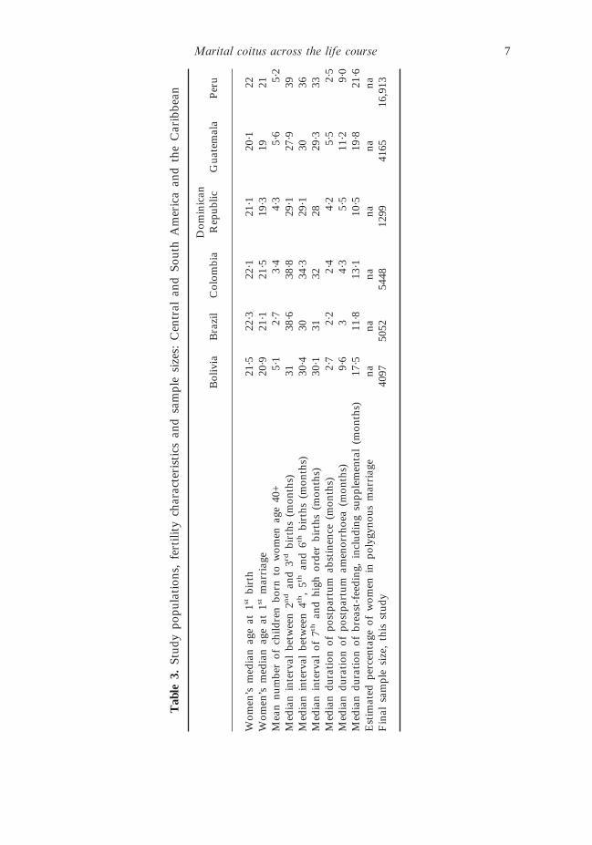
The data for this study were derived from Demographic and Health Surveys (DHS),based on interviews conducted with representative samples of reproductive age womenfrom all major developing world regions. Details of how these data were collectedand access to the databases are provided by the Macro International website(www.measuredhs.com). Country databases were included in this study if (a) therewas a sufficiently large sample of married women still in their first marriage for theform of modelling proposed, (b) data were collected on either the more recent DHS+or DHS III interview schedules (if both datasets were available for a country thenthese were combined), and (c) the variables of interest were available (for example,data on husband’s age is not available in all cases). This resulted in selection ofdatasets for nineteen countries from three world regions (Asia, Africa, the Americas).These countries have diverse fertility profiles and related reproductive practices, as isshown in Tables 1–3.

Limiting of the analyses to non-abstaining women makes the results much morereadily interpretable, and was feasible given the very large sample sizes. Thus, analysiswas then limited to only those women in each country sample who were at risk ofmarital coitus occurring: women who were currently married, whose husband wascurrently resident in the household, and who were not currently abstaining. Coupleswere defined as sexually abstinent if they had not had intercourse within the last year,regardless of the reason, and/or if they had not had sex since their last birth. Theanalyses thus exclude long term abstainers. Additionally, only women in their firstmarriages were included. This resulted in a total sample of 91,744 women for allnineteen countries combined, with sample sizes for each country ranging between 938and 16,913 (see bottom of Tables 1–3 for details).

Statistical analyses

The dependent variable in the model is ‘coital frequency’, measured as the time sincelast intercourse and modelled as a probability of coitus occurring on any given day.In DHS survey rounds, sexual frequency estimates are determined by the question:‘when was the last time you had sexual intercourse?’, with responses recorded asnumber of days, weeks, months or years ago. This is considered a relatively reliablemeans of eliciting such data in interview settings (Becker & Begum, 1994), and also

Marital coitus across the life course 3

provides a fairly simple way to consider statistically and so to model probability ofcoitus. These data were converted to a continuous variable of days since lastintercourse for the analyses. This resulted in clumping above reports of one week (twoweeks=14 days and 2 months=61 days, for example); it is reasonable to assume thiswill result in some lack-of-fit to the model, but should not affect the interpretation ofthe results. This measure of days since last intercourse then provided the basis forestimating the variable used in the analysis: probability of a woman having coitus onany given day.

The predictor variables in the model are woman’s age in years, marital durationin years, husband’s age in years, time since last birth (months), parity of the last birth,number of living children, whether the woman is experiencing postpartum amenor-rhoea, whether the woman is breast-feeding, whether the woman is pregnant andduration of pregnancy, and whether the woman has married within the precedingtwelve months. Number of living children was converted to categories of no children,one child, two or three children, and four or more children, as has been the fashionis previous studies of the relationship between number of children and coitalfrequency (e.g. James, 1974; Rao & DeMaris, 1995). Current duration of pregnancywas categorized by trimester. It should be noted that women may not report they arepregnant until well into the first trimester, and accordingly the sample sizes forwomen reporting first trimester of pregnancy are relatively small.

Statistically, a ‘honeymoon effect’ was considered to occur in a population if anindictor variable that has value 1 if married for one year or less, 0 for more than oneyear, combined in a model with number of years married, shows a significant andextra effect that is not consistent with the rate of change over the rest of the marriageduration. It is important to note that the DHS datasets contain few data reportingfrequency of sex in women under eighteen years of age, even though in many of thesecountries women often or even typically marry before this (see Tables 1–3). Thus thesexual behaviour during the honeymoon period of women who marry at very youngages cannot easily be examined.

A GLM was selected as the most appropriate way to determine the overall andspecific country patterns of change in marital coitus with time, given cross-sectionaldata. The probability of coitus on any given day is assumed to be a logistic functionof the various predictor variables, and the number of days since last intercourse ismodelled as a geometric random variable based on this probability. Thus theregression coefficients may be interpreted similarly to those for logistic regression, asthe effect of the variable on the log-odds of coitus. Technical details may be foundin the Appendix.

Procedurally, variables for the model were chosen using the entire dataset (allcountries together, N=91,744) and included only those that entered the model withp<0·005. This model was used for each country’s analysis, though some variablesmight not be significant predictors in all countries. The link function for the GLMis quadratic in the variables ‘years married’ and ‘wife’s age’; the variable ‘husband’sage’ affects the log-odds only linearly, as the quadratic term was not statisticallysignificant. Other highly significant predictors of coital frequency are pregnancystatus, number of months since last birth, number of children, whether the woman iscurrently breast-feeding, and the ‘honeymoon’ variable. The inverse of the number of


months since the last birth is used in the link function, since this effect might beassumed to be large at first and then tapering as the variable increases. There issome natural confounding between the last birth variable and the breast-feedingvariable, as women are more likely to be breast-feeding in the months after thebirth, but in such a large dataset the model can separate these effects quiteefficiently.

One important consideration in developing the model, as discussed above, isstatistically dealing with the relationships between coital frequency, wife’s age,husband’s age and duration of marriage. If it were found that coital frequencydeclined significantly as a function of marriage duration, then the substitution of themarriage duration variable with wife’s age is expected to produce the same significantdecline, since marriage duration and wife’s age are increasing at the same rate. Todetermine which of the three time variables (marriage duration, wife’s age andhusband’s age) most influence coital frequency, these variables must be included in thesame model. However, the interpretation of the effects of these variables is thenintricate. The standard interpretation of a regression coefficient is that it representsthe effect of a variable on the response, when the values of the other variables areheld constant. While it does not make sense to think of a wife’s age as increasingwhile her husband’s age is held constant, coital frequency may be compared acrosscouples with varying wife’s age but the same husband’s age. For this reason, a large,

Table 1. Study populations, fertility characteristics and sample sizes: Asia

Bangladesh Kazakhstan Nepal Philippines

Women’s median age at 1st birth 17–19 22·4 20 22·8Women’s median age at 1st marriage 15 21·2 16·6 21·6Mean number of children born to womenage 40+

5·6 2·9 5·7 4·4

Median interval between 2nd and 3rd births(months)

40·6 34·6 31·4 26·6

Median interval between 4th, 5th and 6th

births (months)37·7 35·4 32·3 29·9

Median interval of 7th and high order births(months)

35 34·7 32·2 28·3

Median duration of postpartum abstinence(months)

7·9 1·9 2·2 2·3

Median duration of postpartumamenorrhoea (months)

2·0 6·2 11·1 5·5

Median duration of breast-feeding,including supplemental (months)

30·1 7·1 32·8 14·1

Estimated percentage of women inpolygynous marriage

na na 5 na

Final sample size, this study 6276 4377 11,027 6336

Country figures in Tables 1–3 are based on basic DHS survey documentation and final countryreports (all available from www.measuredhs.com).


Tab

le2.

Stud

ypo

pula

tion

s,fe

rtili

tych

arac

teri

stic

san

dsa

mpl

esi

zes:

Afr

ica

Ben

inB

urki

naF

aso

Cam

eroo

nE

thio

pia

Ken

yaM

ali

Mal

awi

Zim

babw

eZ

ambi

a

Wom

en’s

med

ian

age

at1st

birt

h19

·919

·319

1919

·218

·819

19·6

18·7

Wom

en’s

med

ian

age

at1st

mar

riag

e18

·817

·617

·416

·418

·816

·518

19·2

17·1

Mea

nnu

mbe

rof

child

ren

born

tow

omen

age

40+

7·7

7·4

6·2

7·7

7·3

7·6

76·

67·

3

Med

ian

inte

rval

betw

een

2nd

and

3rdbi

rths

(mon

ths)

34·3

33·9

31·5

32·2

29·4

31·1

32·1

36·9

31·3

Med

ian

inte

rval

betw

een

4th,

5than

d6th

birt

hs(m

onth

s)35

·335

·231

·634

·730

·732

·535

·239

·231

·7

Med

ian

inte

rval

of7th

and

high

orde

rbi

rths

(mon

ths)

34·3

35·4

31·5

33·6

30·5

33·7

36·1

36·3

33·9

Med

ian

dura

tion

ofpo

stpa

rtum

abst

inen

ce(m

onth

s)8·

919

·211

·92·

43·

02·

45·

83·

54·

7

Med

ian

dura

tion

ofpo

stpa

rtum

amen

or-

rhoe

a(m

onth

s)11

·715

·910

·719

10·8

11·7

12·7

12·9

11·5

Med

ian

dura

tion

ofbr

east

-fee

ding

,in

clud

ing

supp

lem

enta

l(m

onth

s)22

·326

·918

·225

·521

·122

·624

·318

·820

Est

imat

edpe

rcen

tage

ofw

omen

inpo

lygy

n-ou

sm

arri

age

4555

3314

2043

1719

17

Fin

alsa

mpl

esi

ze,

this

stud

y27

6193

813

8949

3729

5941

4250

0417

6728

57


Tab

le3.

Stud

ypo

pula

tion

s,fe

rtili

tych

arac

teri

stic

san

dsa

mpl

esi

zes:

Cen

tral

and

Sout

hA

mer

ica

and

the

Car

ibbe

an

Bol

ivia

Bra

zil

Col

ombi

aD

omin

ican

Rep

ublic

Gua

tem

ala

Per

u

Wom

en’s

med

ian

age

at1st

birt

h21

·522

·322

·121

·120

·122

Wom

en’s

med

ian

age

at1st

mar

riag

e20

·921

·121

·519

·319

21M

ean

num

ber

ofch

ildre

nbo

rnto

wom

enag

e40

+5·

12·

73·

44·

35·

65·

2M

edia

nin

terv

albe

twee

n2n

dan

d3rd

birt

hs(m

onth

s)31

38·6

38·8

29·1

27·9

39M

edia

nin

terv

albe

twee

n4th

,5th

and

6thbi

rths

(mon

ths)

30·4

3034

·329

·130

36M

edia

nin

terv

alof

7than

dhi

ghor

der

birt

hs(m

onth

s)30

·131

3228

29·3

33M

edia

ndu

rati

onof

post

part

umab

stin

ence

(mon

ths)

2·7

2·2

2·4

4·2

5·5

2·5

Med

ian

dura

tion

ofpo

stpa

rtum

amen

orrh

oea

(mon

ths)

9·6

34·

35·

511

·29·

0M

edia

ndu

rati

onof

brea

st-f

eedi

ng,

incl

udin

gsu

pple

men

tal

(mon

ths)

17·5

11·8

13·1

10·5

19·8

21·6

Est

imat

edpe

rcen

tage

ofw

omen

inpo

lygy

nous

mar

riag

ena

nana

nana

naF

inal

sam

ple

size

,th

isst

udy

4097

5052

5448

1299

4165

16,9

13


cross-sectional dataset is necessary to attempt to determine which of the timevariables is most important in modelling changing coital frequency.

Where frequency of marital coitus changes over time, all three measures of thetime variable increase at the same rate. Yet the sentence ‘frequency of coitus declineswith duration of marriage’ suggests a different interpretation, and thus theory ofunderlying causes of change, than ‘frequency of coitus declines with husband’s age’.Determining if one of these time variables is the cause of change in coital frequencyis not possible; however, with large datasets it is possible to determine which of thethree variables is most strongly related to or the strongest predictor of temporalchanges in coital frequency. If longitudinal data were available for a given couple, thevariables ‘marital duration’, ‘wife’s age’ and ‘husband’s age’ would be completelyconfounding in any model, since they are exact linear functions of each other. In thelarge, cross-sectional dataset used here, these three variables are highly but not exactlycorrelated. In a principal component analysis (PCA) of the three variables, separatelyby country, the first (standardized) principal component is evenly weighted on allthree variables and explains between 88 and 94% of the total variation. The secondprincipal component may be described as a contrast between husband’s age andmarriage duration; this is consistent across all nineteen countries, probably becausethe DHS samples were selected based in part on the woman’s age. The highcorrelation between the time variables seen in PCA implies that there is one mostimportant dimension underlying these three variables, and that if frequency is seen todecline with only one time variable, such as wife’s age, in the model then it will alsodecline when husband’s age is the only time variable in the model. Standard practiceis to choose only one dimension to include in the model, either a single variable ora linear combination of the variables such as the first principal component. However,this dataset is sufficiently large to see separate effects of the three time variables, incountries where these might exist. The combination of these effects described by themodel comprises the variation over time.

Results

Descriptively, there is variation in the overall rate of coitus across countries, and inthe absolute and relative amount of change in coitus over time, as can be seen inTable 4. On the basis of the results of the regression analysis, it is found that maritalsexual frequency generally declines over time. Significant reductions were seen in allcountries except one: although some decline in Burkina Faso is evident, it proved tonot be statistically significant. Significant honeymoon effects, defined as occurringwhen those in the first year of marriage are having more frequent sex than would bepredicted based on age and marriage duration alone, are observed in Benin, Brazil,Ethiopia, Kazakhstan and Mali. The coefficient in all these cases is positive, indicatinghigher frequency in the first year of marriage. The honeymoon variable is also asignificant predictor in Burkina Faso, but here it has a negative effect, indicatingsignificantly lower frequency in the first year of marriage. In the remaining countriesthere is no honeymoon effect apparent.

The model described substantial differences across the populations in whether it ismarriage duration, women’ age or husband’s age that best predicts temporal change


in the risk of coitus occurring, once the other two time variables are controlled. Theserelationships are complex: for example, in Nepal, where N is a substantial 11,027, thelog odds of coitus occurring on any given day is seen to decrease quadratically withmarital duration, linearly with husband’s age; and further increases quadratically withwife’s age up to a peak at age 31, then declines. Each of these effects is statisticallysignificant with p<0·001. In contrast, the effect of husband’s age and marriageduration on coital frequency in Bolivia (N=4097) is not statistically significant oncewife’s age is included in the model, although any of the three variables is a significantpredictor in the absence of the other two. This implies that the strongest predictor ofchange in coital frequency in Bolivia is wife’s age (p<0·0001), and here a peak is alsoseen at age 31. In Cameroon, husband’s age is the strongest predictor (p<0·0001);neither marital duration nor wife’s age remains significant if husband’s age is in themodel. There is a strong linear decrease in log odds of coitus with husband’s age inthis country. The patterns in Malawi and Mali are very similar.

Table 4. Probability of coitus on any day for all countries early and late in the lifecourse, comparing scenarios assuming set age and marital duration

Daily risk of coitus

Earlier in thelife course

Later in thelife course

Absolutechange

Relative decline(%)

Dominican Republic 0·161 0·053 0·108 67·1Brazil 0·147 0·063 0·084 57·1Malawi 0·146 0·069 0·077 52·7Kazakhstan 0·137 0·040 0·097 70·8Ethiopia 0·131 0·038 0·093 71·0Zimbabwe 0·128 0·068 0·060 46·9Philippines 0·127 0·033 0·094 74·0Colombia 0·122 0·041 0·081 66·4Kenya 0·122 0·056 0·066 54·1Zambia 0·119 0·059 0·060 50·4Peru 0·104 0·038 0·066 63·5Guatemala 0·100 0·050 0·050 50·0Nepal 0·098 0·040 0·058 59·2Cameroon 0·095 0·026 0·069 72·6Bolivia 0·079 0·028 0·051 64·6Benin 0·071 0·020 0·051 71·8Bangladesh 0·068 0·054 0·014 20·6Mali 0·067 0·042 0·025 37·3Burkina Faso 0·065 0·050 0·015 23·1

Earlier in the life course: Assumes a non-pregnant women at age 20, just married with nochildren, with husband 5 years her senior.Later in the life course: Assumes a non-pregnant women at age 50, married for 30 years, witha husband 5 years her senior, who has had three children.Coital frequency is estimated as the risk of the couple having coitus on any given day.


Wife’s age was a significant predictor of change in ten of nineteen countries, wherethe log-odds of coitus varies quadratically (p<0·01) in wife’s age in seven of these.This describes a peak in coital frequency that is statistically explained by the wife’sage rather than either of the other time variables. The peak occurs close to 30 yearsof age in all seven countries: Bolivia (31 years), Brazil (28), Colombia (31), Guatemala(27), Kazakhstan (31), Nepal (31) and Peru (33). In Bangladesh, there is quadraticeffect in wife’s age, but the coefficient of the quadratic is positive, which indicates thatcoital frequency declines with wife’s age more rapidly than merely linearly, and thereis no peak. In Benin, Ethiopia and Mali, the log-odds of coitus decreases linearly withwife’s age; i.e. while there is a significant effect of wife’s age, it does not include asignificant peak.

In eleven of the nineteen countries, husband’s age was a significant predictor(p<0·01). There is a decline in coital frequency due to husband’s age in Brazil,Cameroon, Colombia, Dominican Republic, Ethiopia, Kenya, Malawi, Mali, Nepal,Peru and the Philippines.

Marital duration was a significant predictor of life course decline in coitus in sevencountries. In the Philippines, there is a significant quadratic effect of marital durationwith a peak occurring at just over two years married. In Mali and Nepal, there is asignificant peak due to marriage duration occurring at 10 years married. The log-oddsof coitus decreases quadratically for married couples in Colombia, and linearly forKenya and Peru. Log-odds of coitus actually increases linearly in Brazil, but as thereare negative effects of husband’s age, as well as significant effects from the wife’s age,these combine to give an overall life course decline.

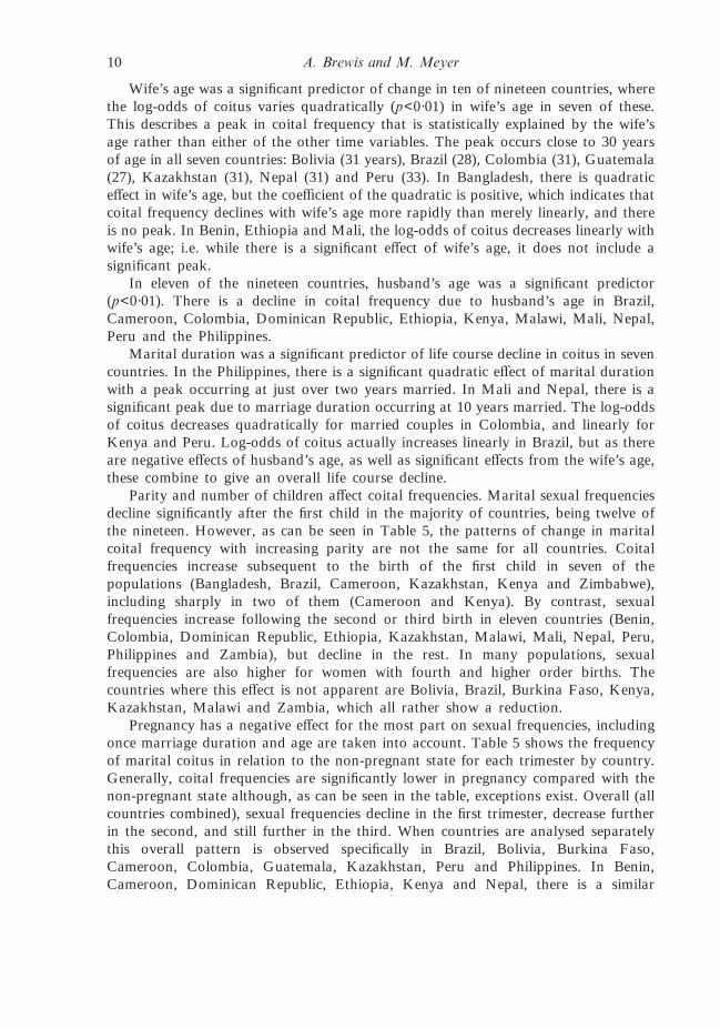
Parity and number of children affect coital frequencies. Marital sexual frequenciesdecline significantly after the first child in the majority of countries, being twelve ofthe nineteen. However, as can be seen in Table 5, the patterns of change in maritalcoital frequency with increasing parity are not the same for all countries. Coitalfrequencies increase subsequent to the birth of the first child in seven of thepopulations (Bangladesh, Brazil, Cameroon, Kazakhstan, Kenya and Zimbabwe),including sharply in two of them (Cameroon and Kenya). By contrast, sexualfrequencies increase following the second or third birth in eleven countries (Benin,Colombia, Dominican Republic, Ethiopia, Kazakhstan, Malawi, Mali, Nepal, Peru,Philippines and Zambia), but decline in the rest. In many populations, sexualfrequencies are also higher for women with fourth and higher order births. Thecountries where this effect is not apparent are Bolivia, Brazil, Burkina Faso, Kenya,Kazakhstan, Malawi and Zambia, which all rather show a reduction.

Pregnancy has a negative effect for the most part on sexual frequencies, includingonce marriage duration and age are taken into account. Table 5 shows the frequencyof marital coitus in relation to the non-pregnant state for each trimester by country.Generally, coital frequencies are significantly lower in pregnancy compared with thenon-pregnant state although, as can be seen in the table, exceptions exist. Overall (allcountries combined), sexual frequencies decline in the first trimester, decrease furtherin the second, and still further in the third. When countries are analysed separatelythis overall pattern is observed specifically in Brazil, Bolivia, Burkina Faso,Cameroon, Colombia, Guatemala, Kazakhstan, Peru and Philippines. In Benin,Cameroon, Dominican Republic, Ethiopia, Kenya and Nepal, there is a similar


pattern except that coital behaviour in the first trimester is not significantly differentfrom the non-pregnant state. In Zimbabwe decline is evident only in the thirdtrimester. Exceptions to the overall pattern are seen: in Bangladesh coitus is morecommon in the third trimester, and there is a significant rise in coital rates in the firsttrimester from a non-pregnant state reported by women in three African countries:Malawi, Mali and Zambia.

Figure 1 takes these country differences into account to provide country-specificillustrations of the relationship between marriage duration and coital frequency,including all the covariates in the model. These scenarios assume a hypotheticalwoman, married at median age for that sample to a man of the same age, who thenfollows a life course in which her age at her first birth, numbers of birth, birthspacing, duration of breast-feeding and postpartum amenorrhoea and abstinenceapproximate median values for that country (with these values taken from Tables 1–3and rounded). For example, in the Bangladeshi scenario, the change in marital coitusby marriage duration is modelled for a hypothetical woman who marries at 15, hasa first child 15 months later, breast-feeds for 24 months, has a second child 42 monthsafter the first, breast-feeds for a further 32 months, has a third child at 100 months,and breast-feeds an additional 32 months after that birth, and so on.

Table 5. Differences in frequency of coitus by parity

Current number of children

1 2–3 R4

Bangladesh / / /Benin b / /Bolivia / / bBrazil / / /Burkina Faso b / /Cameroon a b aColombia / / /Dominican Republic / / /Ethiopia a b /Guatemala / b /Kazakhstan / / bKenya / b /Malawi b / /Mali / / bNepal b a /Peru / / /Philippines / / aZambia / / /Zimbabwe / b a

/ no significant change from lower parity; a frequency is significantly lower than previousparity category; b frequency of coitus is significantly higher than previous parity category.Significance is based on p<0·01.


Discussion

There is significant decline in marital coital frequency across the life course in allcountries, except one. Burkino Faso does show evidence of decline, but it is notstatistically significant: it also has the smallest sample size of all the countries includedin this analysis, and given a larger sample the decline may have proved significant.Therefore, based on very large samples from nineteen countries, a basic conclusion isthat these samples suggest that marital sexual frequency universally declines across thelife course.

These analyses help clarify whether women’s age, husband’s age, or marriageduration best explains this general pattern of life course change: the findings are thatthere are differences across populations in whether marriage duration, husband ageand women’s age best predicts coital frequency across time. If marriage duration isused as the only time variable in the model, it has a significant effect (linear orquadratic) on the log-odds of coital frequency for all countries but Burkina Faso andBangladesh. If wife’s age is used as the only time variable, significant effects are seenin all countries but Burkina Faso. When husband’s age is the only time variable, it

Table 6. Differences in coital frequency by pregnancy trimester compared withnon-pregnant state

Pregnancy trimester

1st 2nd 3rd

Bangladesh / / aBenin / b bBolivia b b bBrazil b b bBurkina Faso b b bCameroon b b bColombia b b bDominican Republic / b bEthiopia / b bGuatemala b b bKazakhstan / b bKenya / b bMalawi a / bMali a / bNepal / b bPeru b b bPhilippines b b bZambia a / bZimbabwe / / b

/ no significant change from non-pregnant state; a frequency is significantly lower thannon-pregnant state; b frequency of coitus is significantly higher than non-pregnant state.Significance is based on p<0·01.


Fig. 1.


Fig. 1. Continued


significantly predicts coital frequency log-odds in all countries but Burkina Faso.Thus, in most countries the effect of time on coital frequency can be seen with anyof the three time variables. When they are all used together in the model, thedominant predictor(s) emerge, and these vary by country. The summary finding in

Fig. 1. Continued

Fig. 1. Representation of the modelled relationship between marriage duration andcoital frequency for each country. Each graph depicts predicted coital frequency fora ‘typical’ but imaginary woman in that country sample. These life course scenariosassume a hypothetical woman who married at the median age of women in thatcountry sample, married a man of the same age, who then follows a life course inwhich her age at her first birth, numbers of birth, birth spacing, and durations ofbreast-feeding, postpartum amenorrhoea and abstinence are median values for hercountry (values are taken from Tables 1–3 and rounded). The successive troughs andspikes indicate the effects of increasing parity: troughs generally represent theoccurrence of pregnancy and the immediate postpartum period, and spikes the patternbefore the onset of the next pregnancy and birth.


this regard is that there is no especially dominant predictor detectable in allcountries.

However, husband’s and wife’s age operate differently in the model in relation tochanging coital behaviour over time. There are no countries in which instances ofsexual frequency increase with husband’s age whether marriage duration and women’sage are controlled for or not. By contrast, women’s age can have a positive effectinitially in many countries (and in all countries combined) on coital frequency oncemarriage duration and husband’s age are controlled for. It is particularly curious thatthis pattern is seen in all the Latin American countries. This finding that femaleageing is not necessarily associated with declining coital behaviour once other factorsare taken into account, fails to support assertions that biological ageing is thedominant factor explaining negative age-related changes in coital behaviour (such asUdry & Morris, 1978, and Udry et al., 1982). However, the vast majority of thesample wives (over 90%) were younger than their husbands, sometimes much younger;different trends might appear in populations where the couple’s ages are roughly thesame; for example, the peak might be found at a higher wife’s age if the husbandstend to be younger.

Other findings confirm that pregnancy and successive births can, but need notalways, be associated with the decline of coital frequencies. In fact, in contrast to thepattern often observed in US samples (Rao & DeMaris, 1985), many countriesshowed an increase in coital frequency with increasing parity, including after the firstbirth. Rao & DeMaris (1985) proposed that the arrival of children additional to thefirst helps entertain the existing children reducing the emotional and practical toll ofparenting on the couple, or perhaps that the novelty of parenting may wear off overtime, allowing more time and energy for sexual activity. This explanation seems weakwhen faced with a range of countries with culturally varied approaches to parentingand very different sexual and emotional contexts of marriage. Perhaps a reversal ofthis cause-and-effect is possible, where those who tend to have more sex also tend tohave more children, especially in developing countries where effective contraceptiveuse rates are lower and fertility rates are higher. The finding that pregnancysuppresses coital rates temporarily in most countries (although not in every case) isnot surprising, but does underline the importance of controlling for frequency ofpregnancy in models that compare lifetime coital frequency patterns across popula-tions. Without this taken into account country differences in overall fertility rates, forexample, could mask underlying differences in marital coital patterns. (The same basicargument could apply to models examining within-population heterogeneity of coitalfrequency, which should also attempt to control for women’s pregnancy status.)

A significant finding is that many countries do not have a significant ‘honeymooneffect’, meaning that coital frequencies in the first year of marriage are notsignificantly higher than would be predicted based on age and marital duration alone.Honeymoon effects have been little studied by demographers: perhaps the assumptionthat they are a normal feature of populations means there has been little attempt tounderstand where and when they might not occur. It is notable, although perhapsonly coincidental, that the countries in this sample where there was no honeymooneffect are predominantly Catholic. Perhaps the honeymoon effect is reversed wherecouples are using forms of natural family planning such as periodic abstinence to


delay the first pregnancy until the very early marital period has passed. Perhapshoneymoon effects are subdued where proportionately more couples are pregnantwhen they marry, and experience birth and the early postpartum period during thefirst year of marriage. Or maybe in countries where biomedical contraception is notwidely used – whether because it is not readily available or because it is socially orreligiously unacceptable – earlier pregnancy in marriage interrupts the honeymoon.This would be suggested by the finding in this analysis that pregnancy has a strongnegative effect on sexual frequency across second and third trimesters in Catholiccountries. Another possibility is that prevailing marriage practices, such as neolocalversus patrilocal residency rules, may strongly influence the probability of maritalcoitus, especially early in marriage. These all suggest interesting predictions that couldbe tested against micro-demographic data at the local level.

In summary, the model developed here suggests that there is a basic life coursepattern of decline in the frequency of marital coitus, that a honeymoon effect is seenonly in some cases, and that there is no single underlying temporal variable (men’sageing, women’s ageing or increasing marital duration) that best explains decline overtime in all countries, but together they do.

References

Becker, S. & Begum, S. (1994) Reliability study of reporting of days since last sexualintercourse in Matlab, Bangladesh. Journal of Biosocial Science 26, 291–299.

Birren, J. (1968) Aging: psychological aspects. In Sills, D. (ed.) International Encyclopedia of theSocial Sciences, vol. 1. MacMillan, New York, pp. 176–196.

Goldman, N. & Montgomery, M. (1989) Fecundability and husband’s age. Social Biology 36,146–166.

Goldman, N., Westoff, C. & Paul, L. (1985) Estimation of fecundability from survey data.Studies in Family Planning 16, 252–259.

Gould, J. (1972). Comment. Current Anthropology 13, 249.James, W. H. (1974) Marital coital rates, spouses’ ages, family size and social class. Journal of

Sex Research 10, 205–218.James, W. H. (1979) The causes of decline in fecundability with age. Social Biology 26,

330–334.James, W. H. (1981) The honeymoon effect on marital coitus. Journal of Sex Research 17,

114–123.James, W. H. (1983) Decline in coital rate with spouses’ age and duration of marriage. Journal

of Biosocial Science 15, 83–87.James, W. H. (1985) Sex ratio, dominance status and maternal hormonal levels at the time of

conception. Journal of Theoretical Biology 114, 505–510.Jasso, G. (1985) Marital coital frequency and the passage of time: estimating the separate

effects of spouses’ ages and marital duration, birth and marriage cohorts, and periodinfluences. American Sociological Review 50, 224–241.

Kahn, J. & Udry, J. R. (1986) Marital coital frequency: unnoticed outliers and unspecifiedinteractions lead to erroneous conclusions. American Sociological Review 51, 734–737.

Kinsey, A., Pomeroy, W., Martin, C. & Gebhard, P. (1953) Sexual Behavior in the HumanFemale. WB Saunders, Philadelphia.

McCullagh, P. & Nelder, J. (1989) Generalized Linear Models, 2nd edn. Chapman and Hall.


Martin, C. E. (1981) Factors affecting sexual motivation in 60–79 year old males. Archives ofSexual Behavior 10, 399.

Nag, M. (1972) Sex, culture, and human fertility in India and the United States. CurrentAnthropology 13, 216–230.

Rao, K. V. & DeMaris, A. (1995) Coital frequency among married and cohabiting couples inthe United States. Journal of Biosocial Science 27, 135–150.

Ruzicka, L. & Bhatia, S. (1982) Coital frequency and sexual abstinence in rural Bangladesh.Journal of Biosocial Science 14, 397–420.

Talmon, Y. (1968) Aging: social aspects. In Sills, D. (ed.) International Encyclopedia of theSocial Sciences, vol. 5. MacMillan, New York.

Trussell, J. & Westoff, C. (1980) Contraceptive practice and trends in coital frequency. FamilyPlanning Perspectives 12, 246–249.

Udry, J. R. (1980) Changes in the frequency of marital intercourse from panel data. Archivesof Sexual Behavior 9, 319–335.

Udry, J. R., Deven, F. & Coleman, S. (1982) A cross-national comparison of the relativeinfluence of male and female age on the frequency of marital intercourse. Journal of BiosocialScience 14, 1–6.

Udry, J. R. & Morris, N. (1978) Relative contribution of male and female age to the frequencyof marital intercourse. Social Biology 25, 128–134.

Udry, R. (1970) The Social Context of Marriage. Lippincott, Philadelphia.Ware, H. (1979) Social influences on fertility at later ages of reproduction. Journal of Biosocial

Science (supplement) 6, 75–96.Wood, J. (1994) Dynamics of Human Reproduction: Biology, Biometry, Demography. Aldine de

Gruyter, New York.

Appendix

Description of the model

There are observations yi, i=1, . ,N, recording the number of days since the lastintercourse, with predictor variables x1i ,. ,xki, such as age (wife’s and husband’s),duration of marriage, family status, fertility status, etc.

Let pi be the proportion of days on which coitus occurs for the ith couple; thisdepends on the predictor variables x1i ,. ,xki. Model pi as in logistic regression, sothat:

pi �exp ��0 � �1x1i � ··· � �kxki�

1 � exp ��0 � �1x1i � ··· � �kxki�,

or equivalently,

�0 � �1x1i � ··· � �kxki � log F pi

1 � piG.

If it is observed whether or not intercourse occurred on the day preceeding theinterview, a logistic regression could be conducted, but the response is the number ofdays since last intercourse: note that this gives more information about coitalfrequency.

A generalized linear model can be constructed that combines a geometric randomvariable with logistic regression. Given pi, the probability that the number of dayssince intercourse yi equals k follows a geometric distribution, that is:


Prob �yi � k� � �1 � pi�k�1pi,

where k can take on positive integer values.Now given data y, . ,jn, the log likelihood can be written as:

l��;y� � �i�1

n

��0 � �1x1i � ··· � �kxki � yi log �1 � exp ��0 � �1 � ··· � �kxki�� .

This can be seen to be a generalized linear model with link function:

� � mean �y� � exp � � ��0 � �1x1i � ··· � �kxki�� 1.

Using standard generalized linear model theory (for reference see McCullagh &Nelder, 1989), one can obtain the maximum likelihood estimators of the parameters�0, . ,�k along with their standard errors. Inference concerning the parametersinvolves asymptotically normal z-statistics and deviance analysis.


marital coitus across the life course - arizona · pdf filepredictor of marital coital...

Documents