HAL Id: halshs-00566843https://halshs.archives-ouvertes.fr/halshs-00566843

Preprint submitted on 17 Feb 2011

HAL is a multi-disciplinary open accessarchive for the deposit and dissemination of sci-entific research documents, whether they are pub-lished or not. The documents may come fromteaching and research institutions in France orabroad, or from public or private research centers.

L’archive ouverte pluridisciplinaire HAL, estdestinée au dépôt et à la diffusion de documentsscientifiques de niveau recherche, publiés ou non,émanant des établissements d’enseignement et derecherche français ou étrangers, des laboratoirespublics ou privés.

Marital fertility and wealth in transition era France,1750-1850Neil Cummins

To cite this version:Neil Cummins. Marital fertility and wealth in transition era France, 1750-1850. 2009. �halshs-00566843�

WORKING PAPER N° 2009 - 16

Marital fertility and wealth

in transition era France, 1750-1850

Neil Cummins

JEL Codes: N33, J13, D31 Keywords: economic history, fertility decline, France,

family economics, wealth, inequality, social mobility

PARIS-JOURDAN SCIENCES ECONOMIQUES

LABORATOIRE D’ECONOMIE APPLIQUÉE - INRA

48, BD JOURDAN – E.N.S. – 75014 PARIS TÉL. : 33(0) 1 43 13 63 00 – FAX : 33 (0) 1 43 13 63 10

www.pse.ens.fr

CENTRE NATIONAL DE LA RECHERCHE SCIENTIFIQUE – ÉCOLE DES HAUTES ÉTUDES EN SCIENCES SOCIALES ÉCOLE NATIONALE DES PONTS ET CHAUSSÉES – ÉCOLE NORMALE SUPÉRIEURE

Marital Fertility and Wealth in Transition Era France, 1750-1850

Neil Cummins, Dept. of Economic History, LSE

n.j.cummins@lse.ac.uk

Abstract

The spectacularly early decline of French fertility is one of the

great puzzles of economic history. There are no convincing

explanations for why France entered a fertility transition over a

century before anywhere else in the world. This analysis links highly

detailed individual level fertility life histories to wealth at death data

for four rural villages in transition-era France, 1750-1850. The results

show that it was the richest groups who reduced their family size

first and that they used ‘spacing’ strategies to achieve this. In cross

section, measures of the environment for social mobility are strongly

associated with the fertility decline. The evidence presented here

demonstrates that socioeconomic status mattered during the early

French fertility decline. This study is a first step towards re-

establishing the French experience as paramount in our

understanding of Europe’s demographic transition.

Section 1: Introduction

Economic explanations for the European fertility transition,

such as demographic transition theory (Notestein 1945), micro

economic theory (Becker 1960, 1991) and more recently unified

growth theory (Galor 2004) have treated the early French fertility

decline as ‘noise’, the extreme tail end of a normal distribution. This

is the intellectual equivalent of treating Britain as the exception in

explaining the Industrial Revolution1. At the time fertility fell (apx.

1800), France was by far the largest country in Europe, excluding

Russia, with a population of almost 30 million people representing

27.7% of the total population of Western Europe (calculated from

Maddison 2003).

This analysis links highly detailed individual level fertility life

histories to wealth at death data for four rural villages in transition-

era France. The period of analysis is approximately 1750-1850 (based

on those who died 1810-70). The study presented here is the first to

analyze the wealth-fertility relationship during the period of the

French fertility decline. The quality of the data collected allows for

an in-depth investigation of the wealth-fertility relationship between

different demographic regimes, the mechanics behind these patterns

and also allows the testing of various hypotheses for why fertility

declined in France.

Background

1 Comparison borrowed from Van de Walle 1974 p.5.

2

Over the past two centuries, fertility in most of the World has

undergone a sustained and seemingly irreversible transition. Today, a

low fertility regime is the norm in the developed world, with some

regions (particularly in Europe) experiencing sub-replacement

fertility. This demographic transition enabled the productivity

advances of the Industrial Revolution to be transformed into higher

living standards and sustained economic growth. Understanding the

revolution in fertility behavior between the Malthusian and the

modern eras has therefore been a central research question. Despite

this interest, researchers of the transition have not approached a

consensus for the causal mechanisms behind the decline of fertility.

The European fertility project (EFP) led by Ainsley Coale at

Princeton University during the 1970s and ‘80s set out to provide an

empirical base for demographic transition theory. However, the EFP

concluded that the decline of marital fertility during the late 19th

century was almost completely unrelated to socioeconomic changes

(Coale and Watkins 1986). Time (the decade of the 1890s), as

opposed to any socio-economic measure, was the best indicator for

the onset of sustained fertility decline. Therefore, the transition was

an ‘ideational change’ and not an economic adaptation. Recent

criticisms have somewhat diluted the authority of the Princeton view.

Brown and Guinnane (2007) argue that the EFP’s conclusions were

biased by the level of aggregation. The sub-national districts used

(departments, counties, cantons etc.) were too large and internally

heterogeneous to be useful as distinct fertility regimes. Further, the

socioeconomic data collected was not the most relevant to parent’s

fertility decisions.

3

The implications for further research are clear: To go beyond

the EFP two issues must be addressed. Firstly, the level of

aggregation, and secondly, the relevance of the socioeconomic data.

The study presented here directly addresses these two concerns via

an individual level analysis of fertility behavior with real wealth

information.

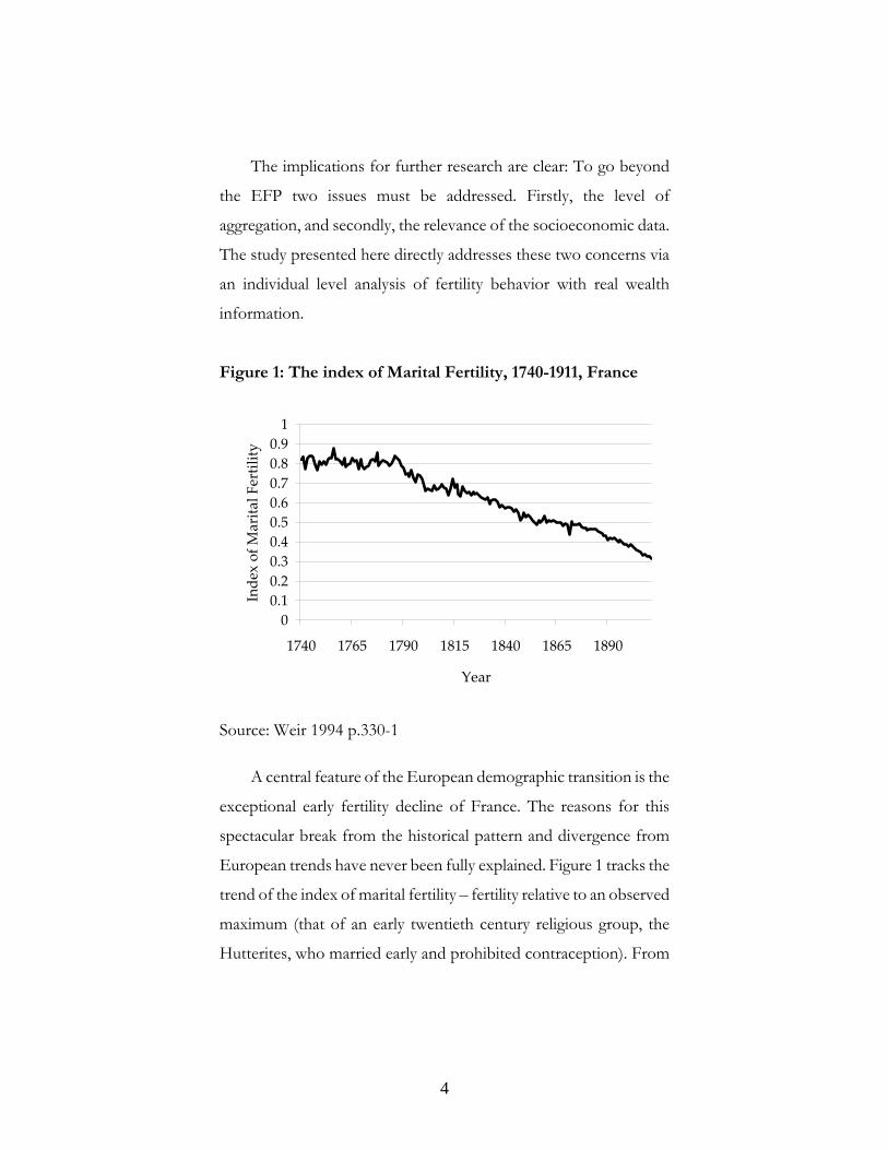
Figure 1: The index of Marital Fertility, 1740-1911, France

00.10.20.30.40.50.60.70.80.91

1740 1765 1790 1815 1840 1865 1890

Year

Inde

x of M

arita

l Fertility

Source: Weir 1994 p.330-1

A central feature of the European demographic transition is the

exceptional early fertility decline of France. The reasons for this

spectacular break from the historical pattern and divergence from

European trends have never been fully explained. Figure 1 tracks the

trend of the index of marital fertility – fertility relative to an observed

maximum (that of an early twentieth century religious group, the

Hutterites, who married early and prohibited contraception). From

4

the late 18th century on, fertility appears to begin a steady and

consistent decline from very high levels (80-90% of the Hutterites)

to very low levels (almost 30% of the Hutterites). Econometric

testing for structural breaks in this series places the transition at

1776. This is nearly a century before anywhere else in Europe

(Belgium (1874)), and 101 years before England and Wales (1877)

(see Cummins 2009 (forthcoming) for details).

There have been relatively few previous studies of the

relationship between economic status and family size at the

individual level for France at this period. Weir, using the Henry

demographic data, examined the income-fertility relationship in

Rosny-Sous-Bois, using tax records for 1747. In a cross-sectional

analysis, he found no difference in marital fertility behavior between

the income groupings. Fertility was high and varied little between his

three income stratifications, although the evidence does suggest a

reproductive advantage for his highest group relative to his lowest

(7.3 to 6.2 births per family respectively) (Weir 1995 p.15). Weir’s

sample size was very small however – he only had a total sample of

47 families to analyze. Hadeishi, with a larger sample size and also

using tax records, studied the town of Nuits in Burgundy from 1744-

1792, and found a positive relationship between marital fertility and

income (2003 p.489). My analysis adds to this literature by linking

pre-existing historical demographic data to new wealth data collected

from various Archives Departmentales in France. The geographic and

socioeconomic scope, along with the sample size, is far greater than

previous studies. This will allow the identification of differential

fertility patterns between socioeconomic strata with greater power.

5

Further, there has been no previous study (to the author’s

knowledge) which has examined the wealth-fertility relationship

during the period of the demographic transition in France (post

1790s).

The rest of this paper is comprised of five sections. Section 2

details the data and its summary characteristics. Section 3 is a detailed

examination of the wealth-fertility associations. Section 4 analyses

the mechanics behind the fertility patterns, while section 5 evaluates

explanations for the French fertility transition. Section 6 Concludes.

Section 2: The Data

The demographic data2 to be analysed is taken from Louis

Henry’s national random sample of 41 villages, roughly covering a

span of over two centuries, from the late 17th to early 19th centuries

(Weir 1995 p.2). This dataset3 is the result of the application of the

techniques of family reconstitution to parish registers and the

fruition of this is a goldmine of individual level information on the

demographic characteristics of historical France. Tens of thousands

of observations record linked births, deaths and marriages. However,

only 20% of the sample recorded the husband’s occupation. As van

de Walle has stated “unfortunately, the population of the parishes

usually is not clearly stratified and most attempts in finding lags in

the dates of fertility decline by socioeconomic groups have failed”

(1978 p.264). To understand the relationship between wealth and 2 I thank George Alter for providing his version of the Henry dataset. 3 The summary papers for the INED French family reconstitution are: Henry (1972), Henry and Houdaille (1973), Houdaille (1976), and Henry (1978).

6

fertility in France at this period, the Henry dataset must be

augmented with more detailed data.

The source for wealth data are the Tables des Successions et

Absences4 (TSA), which are stored in the various Archives

Departmentales in France. The TSAs were originally constructed for

tax purposes and recorded all deaths in a locality, along with detailed

information on date of death, residence, profession, age at death and

marital status. Uniquely, the value of an individual’s estate at death

was noted, with a distinction between cash and property holdings.

Crucially, the TSAs recorded everybody, including those with zero

assets at death (typically coded as “rien”). Almost ¼ of the

individuals in the sample I use fall into this category.

Due to the fact that the property valuation recorded in the TSAs

only covered property held in the locality, it is possible that the

values calculated here are underestimates of the true property wealth

of individuals. However, this bias only affects a small minority of the

sample. According to Bordieu et al, 85% of individuals in the “TRA”

sample (also based on the TSAs) had one property record, leaving

15% with two or more (2004 p.7). Attempts to assess the accuracy of

the wealth information in the TSAs are limited by the fact that “very

few alternative sources exist” (Bourdieu et al. 2004 p.25). However,

Bourdieu et al. test the validity of the Tables against other published

data and find the TSA to yield consistent results (2004 p.26).

4 In English: “Tables of Bequests and Absent Persons” (Bourdieu et al. 2004 p.4).

7

Figure 2: Villages in the Sample

The Henry demographic data set was linked to records from the

Tables des Successions et Absences. The links were based upon name,

profession, sex, age at death and date of death. These criteria serve

to place close to 100% certainty in the accuracy of the links.

Ultimately, four villages were selected on the basis that they were the

best represented after linking. These villages had the properties of

holding a significant number of individuals dying after 1810 (when

the TSAs start to record estimates of wealth), and also having the

TSAs preserved in the relevant Archive Departmental.

The sample covers the fertility experience of individuals who died

roughly between 1810 and 1870 and were born between the 1720s

and the 1820s. The relevant ‘fertile period’ covered is therefore 1750-

1850, roughly speaking. At this time approximately 80% of the

French population lived in rural villages of a similar size to those in

8

the sample (Coale and Watkins 1986 p.235). Fertility decline in

France cannot be understood without understanding what was

happening in these rural villages. However, the sample villages are

only 4 out of perhaps 40,000 villages in France as a whole. The

occupational distribution of these sample villages closely matched

that of the complete Henry Sample (41 villages). The deviations in

representativeness are detailed in the appendix. In order to judge

how representative the demographic regimes in these villages are,

their fertility pattern relative to the National trend is plotted in figure

3.

The National trend in (the index of marital fertility),

presented in figure 3, shows a sharp decline from high levels in the

1780-99 period. Interestingly, the sample villages display a high level

of heterogeneity with respect to the trend in marital fertility. Rosny

has exceptionally high marital fertility which then proceeds to decline

dramatically from 1760-79 period to the post 1780s. Both Cabris and

St Paul have relatively low levels of marital fertility (to the other

villages and the National trend), with a trend towards decline evident

in Cabris from the 1740-1759 period.

gI

The initial trend towards decline in St Paul stalls after 1760, and

along with St Chely, whose fertility remains high throughout, no

trend towards sustained decline is evident. The sample villages

capture the high level of heterogeneity within France with respect to

fertility patterns. Two of the villages – Rosny and Cabris – show

9

Figure 3: The Index of Marital Fertility, by Sample Village,

Contrasted with the National Trend

0.50

0.55

0.60

0.65

0.70

0.75

0.80

0.85

0.90

1740‐1759 1760‐1779 1780‐1799 1800‐1819

Inde

x of M

arita

l Fertility

France Cabris St PaulSt Chely Rosny

clear evidence for decline, while the other two – St Paul and St Chely

– do not share the same pattern. Examining the trend from the

1760-79 period to 1800-1819, we see that fertility in Rosny falls by

nearly 40% and in Cabris by almost 20%. In St Chely and St Paul,

fertility remains relatively constant. Therefore it is possible to

identify two demographic regimes amongst the sample villages, a

high fertility environment and a declining fertility environment. For

the analysis, the data from each village will be pooled and the varying

wealth effects will be tested for by demographic regime.

10

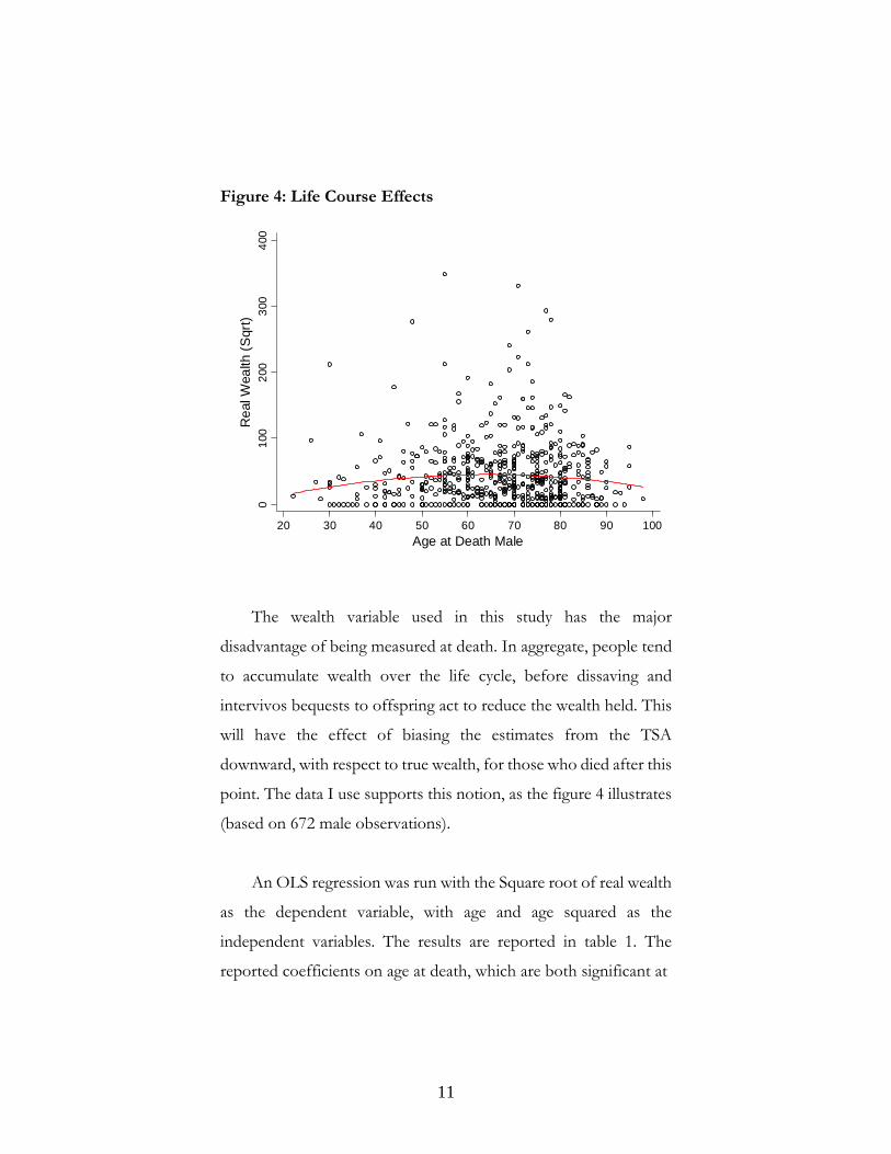
Figure 4: Life Course Effects

010

020

030

040

0R

eal W

ealth

(Sqr

t)

20 30 40 50 60 70 80 90 100Age at Death Male

The wealth variable used in this study has the major

disadvantage of being measured at death. In aggregate, people tend

to accumulate wealth over the life cycle, before dissaving and

intervivos bequests to offspring act to reduce the wealth held. This

will have the effect of biasing the estimates from the TSA

downward, with respect to true wealth, for those who died after this

point. The data I use supports this notion, as the figure 4 illustrates

(based on 672 male observations).

An OLS regression was run with the Square root of real wealth

as the dependent variable, with age and age squared as the

independent variables. The results are reported in table 1. The

reported coefficients on age at death, which are both significant at

11

Table 1: OLS Regression on the Square Root of Real Wealth

Variable Coeff. SE P Age at Death 2.04 0.96 0.03 Age at Death Squared -0.016 0.007 0.03

Constant -20.8 29.5 .48 Adjusted R-Squared 0.004

Observations 672

the 5% level, indicate a turning point age of 63.755, beyond which

the relationship between wealth and age at death turns negative.

There is a possibility that the life course pattern of wealth

accumulation and subsequent decline may blur the true level of

wealth of an individual in the sample. However, I consider this

probability quite small as the slope of the line is so flat. There are no

significant negative associations revealed by the analysis of the

aggregate data between the level of real wealth and age at death. In

total over 60% of the sample died above 64, and taking their value of

wealth at death carries a risk of undervaluation due to the life course

effects. The OLS regression on the square root of real wealth allows

us to calculate an average bias (assuming the true level of wealth is

reached at age 64) based on the average life course relationship

between wealth and age6.

5 Equivalent to the point on the quadratic fit of the wealth and age observations where the slope is equal to zero. Calculated via differentiating the regression equation of the quadratic fit, setting equal to zero, and solving for age at death. 6 These numbers are calculated using the deviation of the regression line from a flat line from age 64 onwards.

12

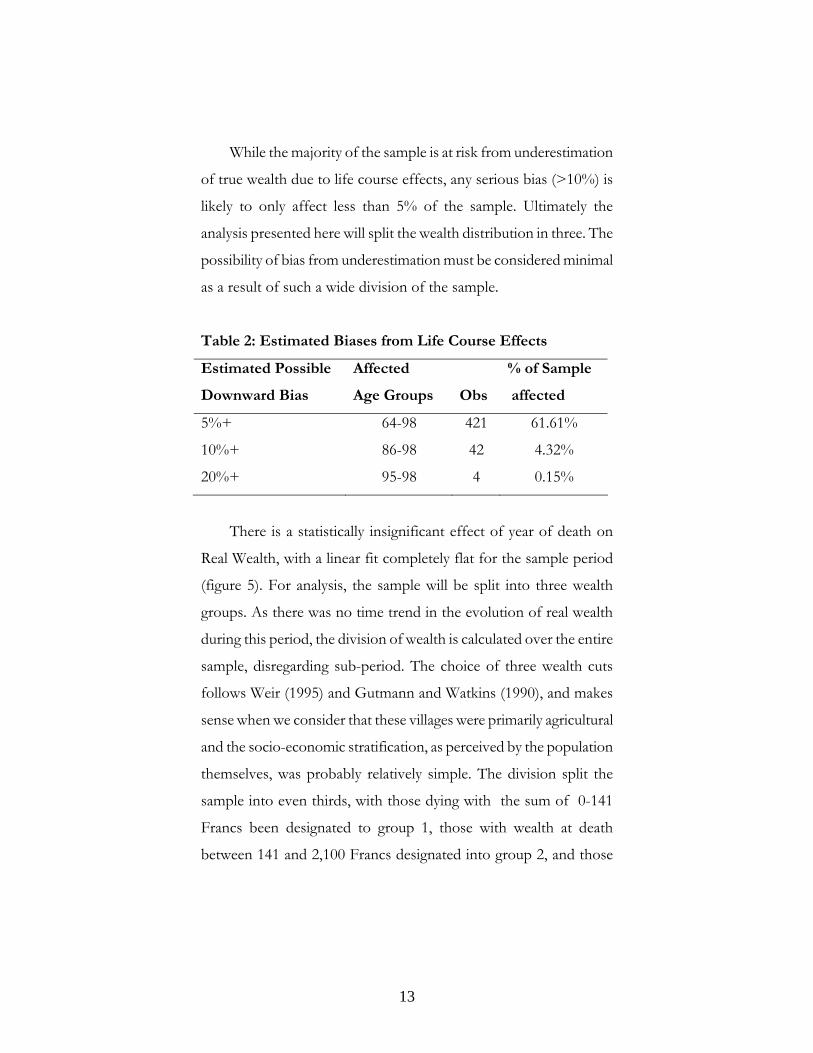
While the majority of the sample is at risk from underestimation

of true wealth due to life course effects, any serious bias (>10%) is

likely to only affect less than 5% of the sample. Ultimately the

analysis presented here will split the wealth distribution in three. The

possibility of bias from underestimation must be considered minimal

as a result of such a wide division of the sample.

Table 2: Estimated Biases from Life Course Effects

Estimated Possible

Downward Bias

Affected

Age Groups Obs

% of Sample

affected

5%+ 64-98 421 61.61%

10%+ 86-98 42 4.32%

20%+ 95-98 4 0.15%

There is a statistically insignificant effect of year of death on

Real Wealth, with a linear fit completely flat for the sample period

(figure 5). For analysis, the sample will be split into three wealth

groups. As there was no time trend in the evolution of real wealth

during this period, the division of wealth is calculated over the entire

sample, disregarding sub-period. The choice of three wealth cuts

follows Weir (1995) and Gutmann and Watkins (1990), and makes

sense when we consider that these villages were primarily agricultural

and the socio-economic stratification, as perceived by the population

themselves, was probably relatively simple. The division split the

sample into even thirds, with those dying with the sum of 0-141

Francs been designated to group 1, those with wealth at death

between 141 and 2,100 Francs designated into group 2, and those

13

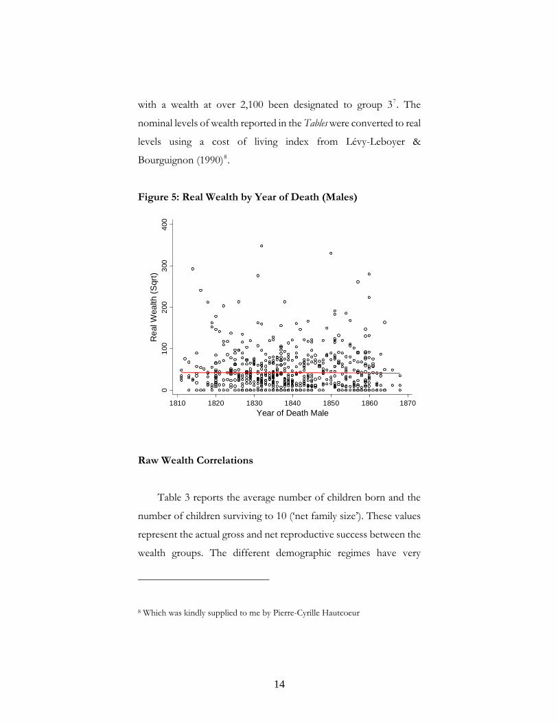
with a wealth at over 2,100 been designated to group 37. The

nominal levels of wealth reported in the Tables were converted to real

levels using a cost of living index from Lévy-Leboyer &

Bourguignon (1990)8.

Figure 5: Real Wealth by Year of Death (Males)

010

020

030

040

0R

eal W

ealth

(Sqr

t)

1810 1820 1830 1840 1850 1860 1870Year of Death Male

Raw Wealth Correlations

Table 3 reports the average number of children born and the

number of children surviving to 10 (‘net family size’). These values

represent the actual gross and net reproductive success between the

wealth groups. The different demographic regimes have very

8 Which was kindly supplied to me by Pierre-Cyrille Hautcoeur

14

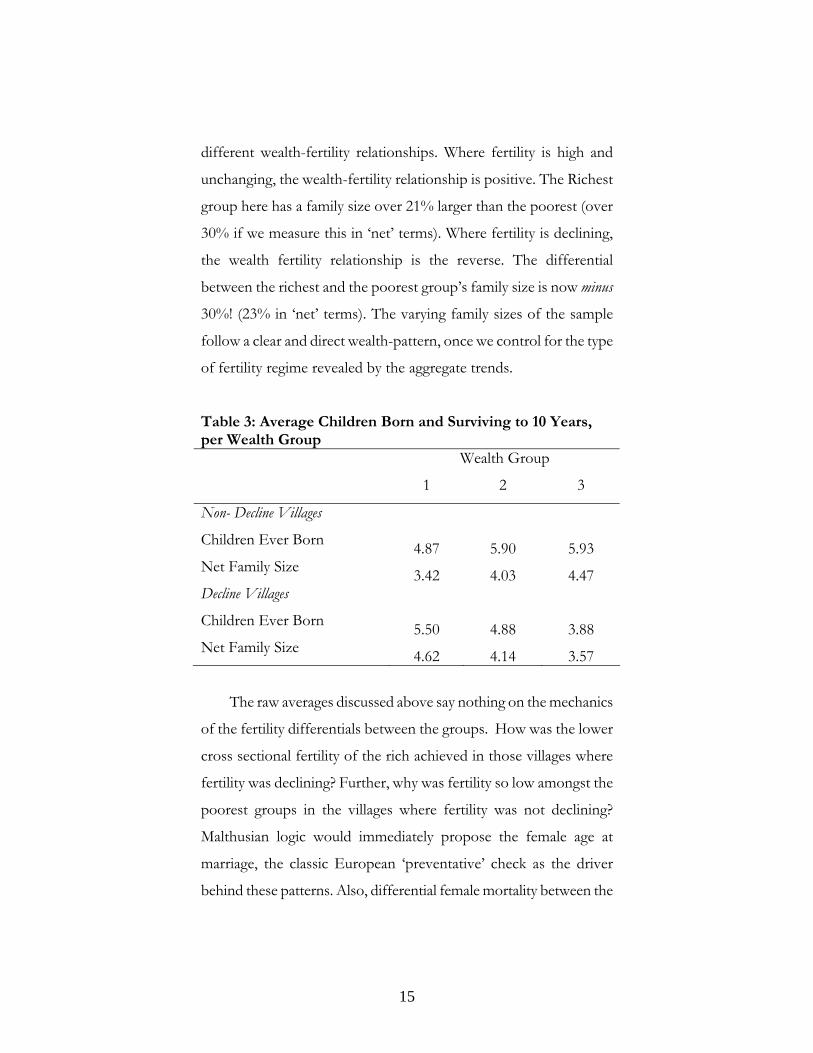
different wealth-fertility relationships. Where fertility is high and

unchanging, the wealth-fertility relationship is positive. The Richest

group here has a family size over 21% larger than the poorest (over

30% if we measure this in ‘net’ terms). Where fertility is declining,

the wealth fertility relationship is the reverse. The differential

between the richest and the poorest group’s family size is now minus

30%! (23% in ‘net’ terms). The varying family sizes of the sample

follow a clear and direct wealth-pattern, once we control for the type

of fertility regime revealed by the aggregate trends.

Table 3: Average Children Born and Surviving to 10 Years, per Wealth Group

Wealth Group

1 2 3

Non- Decline Villages

Children Ever Born 4.87 5.90 5.93 Net Family Size 3.42 4.03 4.47 Decline Villages Children Ever Born 5.50 4.88 3.88 Net Family Size 4.62 4.14 3.57

The raw averages discussed above say nothing on the mechanics

of the fertility differentials between the groups. How was the lower

cross sectional fertility of the rich achieved in those villages where

fertility was declining? Further, why was fertility so low amongst the

poorest groups in the villages where fertility was not declining?

Malthusian logic would immediately propose the female age at

marriage, the classic European ‘preventative’ check as the driver

behind these patterns. Also, differential female mortality between the

15

wealth groups could be generating a lot of the variation. Does the

perceived wealth effect act through these channels? The following

section details regressions designed to detect the wealth effects

controlling for these demographic variables and also event dummies

such as the French Revolution.

Section 3: Deconstructing the Wealth Effects

The equations below detail the components of net family size.

Any wealth effects on net family size have to operate through

differentials in these values.

)50,,,min(

*

FAgeMFAgeDMAgeDEU

FAgeMEUMD

CEDMDMFRNetF

CEDCEBNetF

=

−=

−=

−=

Where is net family size, and are children

ever born and died respectively,

NetF CEB CED

MFR is the marital fertility rate,

MD is the duration of the marriage, is the end of the union

(marriage), is the husbands age at death, and

are female age at marriage and death respectively.

EU

MAgeD FAgeM

FAgeD

Further, it can be expected that other forces, operating at the

village level, and also at the national level (for instance the

16

Revolution and the effects of the Napoleonic wars), have a influence

upon individual’s fertility choices . To examine the specific wealth

effects in the sample, a regression framework was established.

The model to be estimated takes the following functional form:

),,,,,,,.( WealthIMNWARsREVFageDFageMDCCEBf ii

Where represents a constant, C D is a fertility regime fixed effect,

represents a measure of infant mortality, and and

are categorical variables representing the Revolution and

Napoleonic wars respectively. The last mentioned ‘event’ variables

were coded relative to year of marriage, with those with a year of

marriage in 1789 or later receiving a Revolution effect, and those

married between 1802 and 1814 receiving a war effect. The

variable is included in the regression as a categorical variable

in order to account for expected non-linearities in the wealth fertility

relationship.

IM REV

NWARs

Wealth

Any analysis of fertility must account for the impact of child

deaths upon parent’s fertility decisions. Further, these child mortality

estimates must take into account the significant likelihood of the

omission of child deaths in the death registers. A popular way to

detect under registration in death records is to examine the frequency

of first name repetition within a family. Typically, later born siblings

would be given the name of a previously deceased child. Houdaille

has conducted an in-depth analysis of the Henry dataset for these

17

features. However, his results are based on the village level and will

tell us nothing on the wealth differentials within the villages with

respect to infant and child mortality. One result that is relevant here

is the completeness of the death records in Rosny, where no under

registration was detected at all (Houdaille 1984 p.88). For this study,

I employed a simple version of this technique. First, I counted up the

number of repeated names within a family. This was then compared

with the number of recorded child deaths. Where the number of

repeated names exceeded the number of child deaths, I corrected the

child deaths upwards to account for the probable omission of a

death from the records. Table 4 reports the corrected and non

orrected values by fertility regime and wealth division.

their rate is half that of

the richest group in the non-decline villages.

ositive

correlation between fertility and mortality (Guinnane et al.

c

There are huge differences in child mortality between the

villages. Within those were fertility is high, child mortality is high too.

Within the villages, child mortality varies to a far less extent, with

almost no differences between the wealth groups where fertility is

high. The wealthiest group in the decline villages have child mortality

far below any other group in the sample, and

Is the decline in fertility related to a reduction in child mortality

at this period? To examine this, I will proceed with a multivariate

regression. There is a probable endogenous relationship between

fertility and infant mortality. Firstly, the number of child deaths can

never exceed the number of births. This induces a p

18

Table 4: Child Mortality (until 10 years) by Fertility Regime

and Wealth Group, Rates per 1000 births

Wealth Group

1 2 3

Non- Decline Villages

Corrected 326.8 342.1 335.1

Uncorrected 283.1 320.6 314.2

Decline Villages

Corrected 201.5 211.0 166.6

Uncorrected 181.2 197.9 162.0

2006 p. 472). Secondly, parents may choose to replace a deceased

infant. Any interpretation of a parent’s gross family size must

therefore factor in the effects of the mortality experience. Following

Guinnane et al., I factor in mortality by including the proportion of

children dead as an independent variable in the regression. This

removes the structural correlation between mortality and fertility but

does not remove the endogenity.

As the dependant variable is a count variable and because the

data is ‘over dispersed’ relative to the Poisson distribution, the

appropriate method is to use negative binomial regression. The

19

Table 5: Negative Binomial Regressions on Children Ever

Born

Variable Coefficient

(Standard Error) Demographic variables Age at Marriage, Female -0.038***

(0.005) Age at Death, Female 0.035***

(0.004) Proportion of Children dead 0.269**

(0.001) Event variables Revolution -0.149**

(0.059) Napoleonic Wars -.043

(0.054) Wealth Effects Wealth Group1 (ref.) 0 Wealth Group2 0.181*

(0.049) Wealth Group3 0.145

(0.093) Wealth-Fertility Regime Interactions Main Decline Effect 0.085

(0.078) Wealth Group1 (ref.) 0 Wealth Group2 -0.291**

(0.102) Wealth Group3 -0.397***

(0.104) Constant .945***

(0.252) N 411 Psuedo R2 0.088 *** Significant at .001% level ** Significant at .01% level *Significant at .05% level

20

distribution of both gross and net fertility matched the negative

binomial distribution closely, and a comparison with the Poisson

distribution is detailed in the appendix.

Table 5 details the results of a negative binomial regression on

children ever born. Female age at marriage and at death are highly

significant and act in the expected directions9. The proportion of

dead children is also highly significant and it’s effect is large.

Intended to capture the effects of infant mortality, a reduction in this

value decreases the number of children born. The Revolution has a

significant negative effect on fertility, but the Napoleonic wars are

insignificant. The wealth effects are capture by interactions in the

model, and their ‘net’ effects are reported in table 6.

Table 6: Net Wealth Effects on Children ever born Wealth Group

1 2 3

Non- Decline Villages 5.95 7.14 6.88 Decline Villages 6.48 5.81 5.04

The ‘net’ wealth effects on fertility in table 6 are calculated from

the interaction coefficients in the negative binomial regressions. A

constant age at marriage for females (24) and complete life course

fertility (surviving to at least 50) is applied for each wealth group10.

These values represent the wealth effects on fertility ‘net’ of wealth

differentials in age at marriage, death and the proportion of children

9 Women who marry later should have fewer children for biological reasons, and women who die during their reproductive years should have fewer children. 10 The average age at marriage for all women in the sample as a whole was 23.8.

21

dead. Once the net effect is calculated for each wealth group, the

coefficient is exponentiated (as the beta coefficients of the negative

binomial regression are given in logarithms) to give the expected

numbers for each wealth group. These numbers can be understood

as representing the net wealth effects controlling for the factors

listed in the regression, and ignoring the effects of the Revolution

and Napoleonic Wars. In relation to the richest and poorest groups,

the strong positive wealth fertility relationship almost completely

disappears within the non-decline villages. Those in the middle of the

wealth distribution in the non-decline villages – Wealth Group 2,

appear to have the highest marital fertility. Where fertility decline has

already begun, the net wealth fertility relationship is still sharply

negative, with the richest groups having over 22% fewer births. In

summation: Pre-transition villages have a positive wealth-fertility

profile, whereas transition villages have a negative wealth-fertility

profile. This strongly implies that it is the rich, the top third of the

wealth distribution in these rural villages, who are the pioneers of the

decline in French fertility.

As mentioned, one feature the regression results highlight is the

high relative fertility of Wealth Group 2 in the non-decline villages.

One postulation on this feature could be that a proportion of the

richest groups in the non-decline villages are beginning to control their

fertility, but this proportion is too small to move the size of the

wealth effect below that of the poorest group. The quality of the

Henry dataset allows us to examine in fine detail the mechanics of

22

the wealth fertility differentials, and this is described in the next

section.

Section 4: The Mechanics behind the Fertility Patterns

The results from the regressions demonstrate systematically that

economic status mattered during the period of fertility decline in

France. What were the mechanics behind these patterns? The

regressions indicate that both the gross family size correlations with

wealth were independent of marriage age and age at death. The

significant negative association, particularly for Rosny and Cabris

(the ‘decline regime’ villages) for marriages after 1800, must therefore

represent an implementation of fertility limitation strategies within

marriage. There are two ways for couples to control their desired

family size. Firstly, they can stop bearing children once they reach a

certain target family size – this is known as ‘stopping’ behavior .

Secondly, they can increase their birth intervals–‘spacing’ behavior .

The European demographic transition has overwhelmingly been

attributed to ‘stopping behavior ’. However, the aggregation of

those pursuing different reproductive strategies may blur the true

picture. As van Bavel has stated; “research explicitly analyzing

stopping and spacing has hardly ever differentiated between social

status groups” (2002 p.7). The French fertility patterns discussed

here are delineated by economic categories, and this section evaluates

to what extent stopping and spacing can be attributed.

‘Stopping’ Behaviour

23

The Henry demographic dataset allows the calculation of

fertility measures such as Age Specific Fertility Rates, Coale’s index

of marital fertility, the Total Marital Fertility Rate and the Coale and

Trussell fertility control measures “M” and “m” (referred to as big

and little m respectively). The Coale-Trussell parameters are

calculated from the Age Specific Fertility Rates and represent

deviations from the age pattern of ‘natural fertility’. An M value of 1,

and an ‘m’ value of 0 indicate no fertility control. Typically,

researchers look for an ‘m’ value greater than .200 for an

unambiguous sign of a controlling population. M, is harder to

interpret, but may catch ‘spacing’ effects. The appendix details the

statistical derivation of the Coale-Trussell parameters. However,

these measures have been criticized in the literature and are far from

fool proof. Table 7 summarizes the calculated Age specific marital

fertility rates, Total Marital Fertility Rates and the Coale and Trussell

fertility control parameters.

The reproductive advantage of the richest group in the non-decline

villages is emphasized by the high value for M, 0.927. This means

that the richest group here has a fertility level very close to that of

the natural fertility schedule. For the non-decline villages, M has

decreased and the scale of the decrease is, again, closely related to

economic status. The richest have the lowest level of fertility and the

poorest wealth group have the highest. Focusing on ‘m’ – the

parameter indicating significant deviation from a natural age pattern

of marital fertility, the results indicate no unambiguous signs for

stopping behavior in any of the regimes. However, this value is

largest for the richest group in the decline villages (0.146). Despite

24

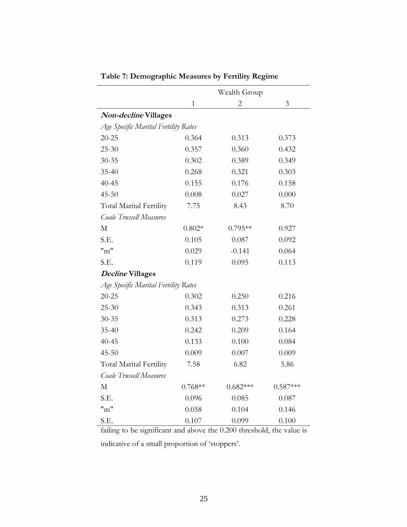
Table 7: Demographic Measures by Fertility Regime

Wealth Group 1 2 3 Non-decline Villages

Age Specific Marital Fertility Rates 20-25 0.364 0.313 0.373 25-30 0.357 0.360 0.432 30-35 0.302 0.389 0.349 35-40 0.268 0.321 0.303 40-45 0.155 0.176 0.158 45-50 0.008 0.027 0.000 Total Marital Fertility 7.75 8.43 8.70 Coale Trussell Measures M 0.802* 0.795** 0.927 S.E. 0.105 0.087 0.092 "m" 0.029 -0.141 0.064 S.E. 0.119 0.095 0.113 Decline Villages

Age Specific Marital Fertility Rates 20-25 0.302 0.250 0.216 25-30 0.343 0.313 0.261 30-35 0.313 0.273 0.228 35-40 0.242 0.209 0.164 40-45 0.133 0.100 0.084 45-50 0.009 0.007 0.009 Total Marital Fertility 7.58 6.82 5.86 Coale Trussell Measures M 0.768** 0.682*** 0.587*** S.E. 0.096 0.085 0.087 "m" 0.058 0.104 0.146 S.E. 0.107 0.099 0.100 failing to be significant and above the 0.200 threshold, the value is

indicative of a small proportion of ‘stoppers’.

25

Another way to detect ‘stopping’ behavior is to look at the

average age women have their last birth. These values are reported

for the regime and wealth group combinations in table 8. The values

are calculated only for those women and their husbands who died

after 50. The mean age at last birth in populations practicing ‘natural

fertility’ is approximately 40-41 years (Bongaarts (1983) as cited by

Kohler et al. 2002 p.28). Amongst the villages where fertility was not

declining, there is no significant variation to report. Age at last birth

is high, around 37-38 years for all wealth groups. For the villages

where fertility was declining, the top 2 wealth groups do show

evidence for ‘stopping’ behavior ; the mean age at last birth is

significantly below that of the other groups in the sample.

Table 8: Age at Last Birth by Fertility Regime

Wealth Group

1 2 3

Non-Decline Villages 37.81 38.62 36.92

Decline Villages 37.80 35.90 35.37

‘Spacing’ behavior

Having established some partial evidence for the presence of

‘stopping’ behavior amongst the wealthiest groups in the sample

villages, the question of ‘spacing’ arises. It is far easier to detect

‘stopping’ behavior in population sub-groups then it is to detect

‘spacing’ behavior. One way to detect spacing is to model the birth

26

intervals directly using a Cox proportional hazards model. The

results will describe the effects of the covariate independent variables

in terms of a ‘hazard rate’, which is defined as the instantaneous

probability of the event in question (in this case a birth), and is

therefore directly related to the length of the birth interval. As the

model is intended to reveal differences in spacing behavior, only

closed birth intervals are used. The formulation of the birth interval

model follows previous analyses by Alter (1988), Bengtsson and

Dribe (2006), Van Bavel (2004a, 2004b) and Van Bavel and Kok

(2004). After consideration of the varying inclusion of demographic

factors in these studies, it was decided to concentrate on those

factors most commonly found to affect the birth interval. This was

done with the aim of producing a parsimonious model which could

capture the wealth effects (if any) on the duration of the birth

interval. The demographic factors included were the age of the

mother (in 5 year age bands), the duration of the marriage, parity,

and the life status of the previous born child. In common with the

analysis by Bengtsson and Dribe, I include shared frailty at the

individual level to control for unobserved family-specific

heterogeneity in the sample (2006 p.736).

The Cox proportional hazards model is based on the following

identity:

)exp()()( 0 xththi β ′=

27

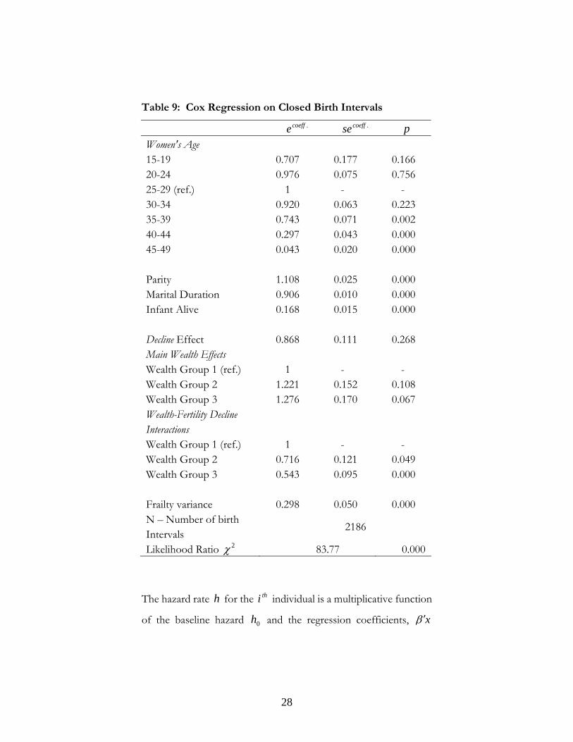
Table 9: Cox Regression on Closed Birth Intervals

.coeffe .coeffse p Women's Age 15-19 0.707 0.177 0.166 20-24 0.976 0.075 0.756 25-29 (ref.) 1 - - 30-34 0.920 0.063 0.223 35-39 0.743 0.071 0.002 40-44 0.297 0.043 0.000 45-49 0.043 0.020 0.000 Parity 1.108 0.025 0.000 Marital Duration 0.906 0.010 0.000 Infant Alive 0.168 0.015 0.000 Decline Effect 0.868 0.111 0.268 Main Wealth Effects Wealth Group 1 (ref.) 1 - - Wealth Group 2 1.221 0.152 0.108 Wealth Group 3 1.276 0.170 0.067 Wealth-Fertility Decline Interactions

Wealth Group 1 (ref.) 1 - - Wealth Group 2 0.716 0.121 0.049 Wealth Group 3 0.543 0.095 0.000 Frailty variance 0.298 0.050 0.000 N – Number of birth Intervals

2186

Likelihood Ratio 2χ 83.77 0.000

The hazard rate for the individual is a multiplicative function

of the baseline hazard and the regression coefficients,

h thi

0h xβ ′

28

(Cleves et al 2004 p.147-8). The great advantage of the Cox

proportional hazard model is that the functional form of , the

baseline hazard, is left unspecified. To account for unobserved

heterogeneity at the individual level a frailty component is included.

Rewriting the hazard:

0h

)exp()()( 0 xthth ii βα ′=

Where iα represents the shared frailty term, assumed to have

mean one and a variance estimated from the data (Cleves et al 2004

p.147-8). This is intended to capture mother specific effects on the

birth interval, constant across all the covariates. As mentioned, the

results reported in table 9 are presented as hazard ratios11. Where the

reported coefficient equals 1, there is no effect of that variable on the

hazard of a birth.

The Cox regressions on the hazard of a birth place attach high

significance to parity, marital duration and the presence of an infant.

Further, the natural fall off in fecundity is reflected by the falling

hazard ratios for age groups past the 25-29 reference category. The

11 The critical proportional hazards assumption was tested by analyzing the Schoenfeld residuals. Using stata’s spthtest revealed that there was a deviation from the proportional hazards assumption in the original formulation of the birth interval model (table 9). Variable by variable analysis indicated that the parity, marital duration and female age grouping variables were driving this violation of the proportional hazards assumption. The analysis was repeated omitting these variables and the new wealth coefficients were compared with the original models. They were extremely similar in both magnitude and significance. Therefore it was decided to report the original model’s results. The proportional hazards assumption was also checked graphically using stata’s stphplot command.

29

Table 10: Net Hazard Ratios and Mean Birth Interval (Months)

by Fertility Regime and Wealth Group

Wealth Group

1 2 3

Non-Decline Villages

Hazard rate 1.000 1.221 1.276 Interval 30.60 27.74 27.57 Decline Villages

Hazard rate 0.868 0.760 0.602 Interval 32.08 33.23 36.41

wealth effects are reported as interactions in the regression table. In

order to calculate the net wealth effects, these values are multiplied,

producing the values reported in table 10. The wealth effects are

large. For the non-decline villages, the hazard ratio for a birth increases

with the wealth category, indicating that the top 2 wealth groups

have significantly shorter birth intervals than the poorest group. For

the decline villages, the opposite is true. The richest here have much

longer birth intervals than the poorest group. The mean birth

interval for each wealth group varies with the hazard rates, and are

also reported in table 10. These results strongly indicate that spacing

played a substantial role in the declining fertility of the richer groups

in the sample. In comparison with the Coale-Trussell measures and

the age at last birth calculations, it appears that it was spacing, not

stopping, which was the primary driver behind the French fertility

decline.

30

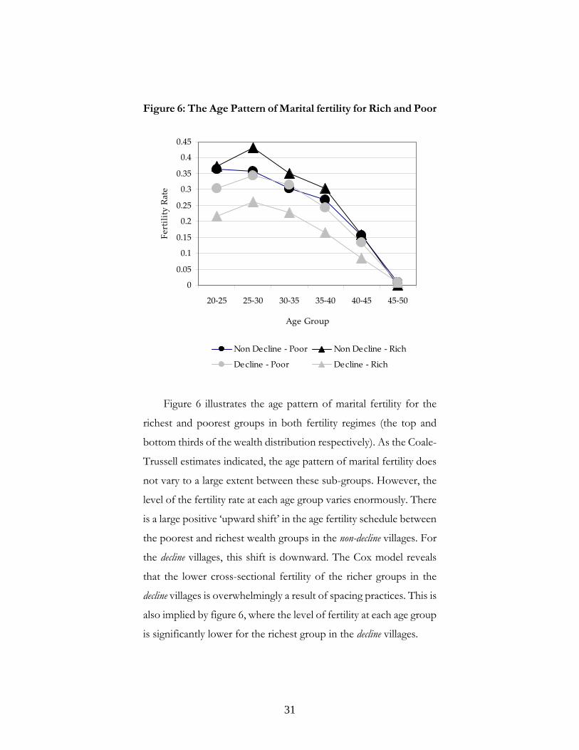
Figure 6: The Age Pattern of Marital fertility for Rich and Poor

0

0.05

0.1

0.15

0.2

0.25

0.3

0.35

0.4

0.45

20‐25 25‐30 30‐35 35‐40 40‐45 45‐50

Age  Group

Fertility Rate

Non Decline  ‐ Poor Non Decline  ‐ Rich

Decline  ‐ Poor Decline  ‐ Rich

Figure 6 illustrates the age pattern of marital fertility for the

richest and poorest groups in both fertility regimes (the top and

bottom thirds of the wealth distribution respectively). As the Coale-

Trussell estimates indicated, the age pattern of marital fertility does

not vary to a large extent between these sub-groups. However, the

level of the fertility rate at each age group varies enormously. There

is a large positive ‘upward shift’ in the age fertility schedule between

the poorest and richest wealth groups in the non-decline villages. For

the decline villages, this shift is downward. The Cox model reveals

that the lower cross-sectional fertility of the richer groups in the

decline villages is overwhelmingly a result of spacing practices. This is

also implied by figure 6, where the level of fertility at each age group

is significantly lower for the richest group in the decline villages.

31

Section 5: Why did fertility decline in France?

Any socioeconomic explanation for early French fertility decline

must consider that England, with a higher level of GDP per capita, a

smaller agrarian sector and a larger urbanization rate lagged behind

French fertility trends by over 100 years. This fact undermines

demographic transition theory, the microeconomic theory of fertility

and unified growth theory12. All of these theories rely on changes in

income, modernization and the labor force structure of the economy

in initiating a substitution of child quantity for quality. None of them

can explain why France was first.

The French themselves have long been preoccupied with the

unusual characteristics of their demographic history. An intellectual

climate obsessed with depopulation and the decline in French

fertility arose around the turn of the 20 century. Van de Walle briefly

discusses this mostly forgotten literature, criticizing its “outdated and

weak statistical content”, and states that the work amounted to a no

more than a series of hypotheses (1974 p.6). Some of these

hypotheses have survived to today, and I focus upon those

forwarded by Tony Wrigley and David Weir13.

12 At least in explaining the fertility transition. 13 Another popular explanation for the French fertility decline is the change in the inheritance laws which accompanied the Revolution. The Napoleonic code replaced primogeniture with equal partition. In order to preserve a concentration of wealth within the family, parents now had to curb their family size, as wealth could not solely be assigned to the eldest male. Chesnais questions this interpretation by pointing out that other countries adopted the same principles but didn’t experience a fertility decline. Further, primogeniture was not practised widely in the North, except amongst the aristocracy, and the South-West of

32

Neo-Malthusian Explanation

Wrigley sees the early adoption of family limitation in France as

“a variant form of the classic prudential system of maintaining an

equilibrium between population and resources to which Malthus

drew attention”. Essentially, the preventative check now operated

through marital fertility directly, and not indirectly through age at

marriage. The net reproduction rate in France from the late 18th to

late nineteenth century was always close to 1, suggesting that the

population was still finely constrained by available resources (Wrigley

p.55 1985). As previously mentioned, almost 80% of the French

population were rural, and nearly 70% lived off farming at the time

of the decline (Chesnais 1992 p.335). Chesnais also points out that

“farming remained primitive” and that there were numerous

indicators of overpopulation (such as increase in wheat prices from

the 1760s-1820s) (1991 p.336). These features certainly lend

themselves to a Malthusian interpretation of the fertility pattern.

The testable implication of this hypothesis, as stated by Weir, is

that there should be a strong positive relationship between real

income and fertility (1984a p.31). However, this ‘neo-Malthusian’

reasoning for the early decline for French fertility fails to be

supported by the individual level data collected in this analysis. If the

restriction on births was a response to an economic constraint, we

France, where primogeniture was common, had relatively low fertility in the Ancien Regime, and followed the same fertility pattern elsewhere post Revolution (1991 p.338).

33

would expect those closest to subsistence to initiate fertility control.

This is clearly not the case for the four villages in the sample. Where

fertility is declining, the wealth-fertility relationship is negative.

Fertility decline here is more pronounced for the richer groups; they

are the first to employ this new variant of the preventative check, but

this is not a ‘neo-Malthusian’ response.

The Revolution

Many scholars (Weir 1984b, and more recently Murphy and

Gonzalez-Bailón 2008) have explicitly linked the Revolution to the

fertility decline. At a superficial (and highly aggregated) level, the

events are near simultaneous (see figure 1). However, econometric

tests on the aggregate fertility rate place the decline in fertility before

the Revolution (1776, see Cummins 2009). Further, it is widely

accepted that many localities began their fertility transition long

before 1789 (Chesnais 1992 p.338). In the data collected for this

analysis, Rosny and Cabris have substantially declining fertility rates

before the Revolution (see figure 3). However, the ideological and

socioeconomic causes of the Revolution were germinating long

before 1789. Could these forces have also contributed to the fertility

revolution as well as the political?

An economic rationale for the decline in French fertility,

associated with the Revolution has been forwarded by Weir. He

states “evidence on fertility by social class is scarce, but tends to

support the idea that fertility control was adopted by an ascendant

“bourgeois” class of (often small) landowners“ (1984b p.613). The

34

Revolution enabled an element of the rural population to increase

their control over the land, while others lost out and became more

reliant on wage labour. For the new rural bourgeoisie, children

became “superfluous as labourers and costly as consumers” (Weir

1984b p.613). The decline of fertility in France in the early to mid

19th century was primarily due to the decline of the demand for

children by this new class. It was only after 1870 when France joined

the rest of Europe in a fertility transition which transcended the

social order (Weir 1984b p.614).

The results of this analysis support Weir’s hypothesis on the French

fertility transition. The new class of landowners created by the

Revolution would certainly lie within the top wealth category as

constructed here. The results clearly show, as Weir expected, that

fertility decline was initiated by this wealthy group. Further, the

effect of the Revolution on family size is large, negative and

significant (see table 11). This is captured in the negative binomial

regressions by coding a categorical variable for those who married

after 1789. A more precise testable implication of Weir’s hypothesis

is that those who have greater property wealth should have the

lowest fertility. Further, the cash component of total wealth at death

should be an insignificant predictor for family size. By splitting the

wealth measures into the property and cash components we can test

for this in the sample data. Once the value is separated, the

distribution is split into even thirds with respect to cash and property

35

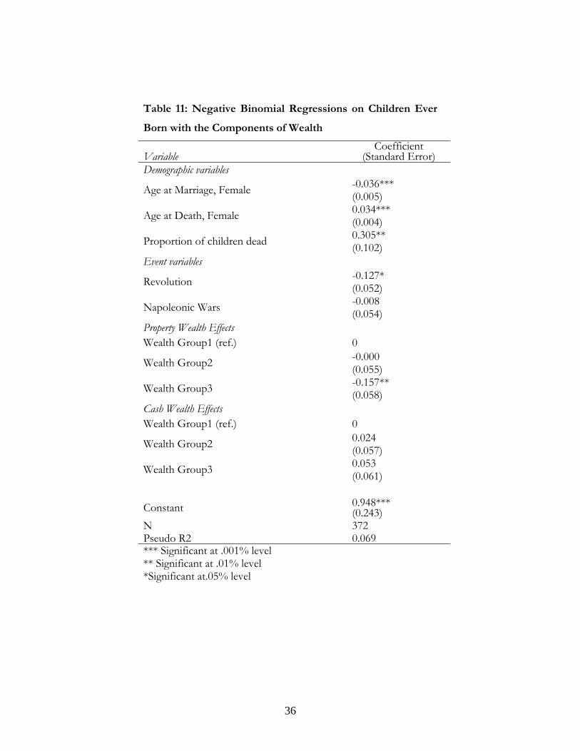
Table 11: Negative Binomial Regressions on Children Ever

Born with the Components of Wealth

Variable Coefficient

(Standard Error) Demographic variables Age at Marriage, Female -0.036***

(0.005)

Age at Death, Female 0.034*** (0.004)

Proportion of children dead 0.305** (0.102)

Event variables

Revolution -0.127* (0.052)

Napoleonic Wars -0.008 (0.054)

Property Wealth Effects Wealth Group1 (ref.) 0

Wealth Group2 -0.000 (0.055)

Wealth Group3 -0.157** (0.058)

Cash Wealth Effects Wealth Group1 (ref.) 0

Wealth Group2 0.024 (0.057)

Wealth Group3 0.053 (0.061)

Constant 0.948***

(0.243) N 372 Pseudo R2 0.069 *** Significant at .001% level ** Significant at .01% level *Significant at.05% level

36

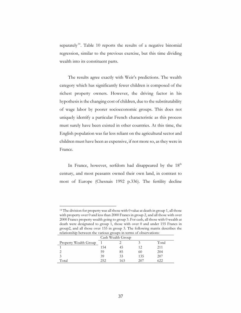
separately14. Table 10 reports the results of a negative binomial

regression, similar to the previous exercise, but this time dividing

wealth into its constituent parts.

The results agree exactly with Weir’s predictions. The wealth

category which has significantly fewer children is composed of the

richest property owners. However, the driving factor in his

hypothesis is the changing cost of children, due to the substitutability

of wage labor by poorer socioeconomic groups. This does not

uniquely identify a particular French characteristic as this process

must surely have been existed in other countries. At this time, the

English population was far less reliant on the agricultural sector and

children must have been as expensive, if not more so, as they were in

France.

In France, however, serfdom had disappeared by the 18th

century, and most peasants owned their own land, in contrast to

most of Europe (Chesnais 1992 p.336). The fertility decline

14 The division for property was all those with 0 value at death in group 1, all those with property over 0 and less than 2000 Francs in group 2, and all those with over 2000 Francs property wealth going to group 3. For cash, all those with 0 wealth at death were designated to group 1, those with over 0 and under 155 Francs in group2, and all those over 155 in group 3. The following matrix describes the relationship between the various groups in terms of observations: Cash Wealth Group Property Wealth Group 1 2 3 Total 1 154 45 12 211 2 59 85 60 204 3 39 33 135 207 Total 252 163 207 622

37

originated amongst the wealthiest of this property holding class15.

According to Chesnais, almost 63% of the population was

represented by landowners and their families in 1830 while the

comparable figure for Britain is 14% (1991 p.337). The widespread

ownership of land amongst the rural population is a unique feature

of the French socio-economic landscape at this time. Because of this,

economic inequality was lower in France than in England during the

19th century (Piketty et al. 2006 p.250). This implies that the

environment for social mobility was more fluid in 18th and 19th

century France than anywhere else in Europe. Arsene Dumont,

writing a century after the onset of the transition, placed social

mobility as the ‘raison de etre’ of the French fertility decline and

termed “social capillarity” as the phenomenon driving the limitation

of family sizes (Dumont 1890). The Revolution served “to increase

the thirst for equality and stimulate the social ambition of families,

both for themselves and their progeny” (Chesnais 1992 p.334). The

old social stratifications under the Ancien Regime, where hereditary

rights had determined social status, were weakened by the

Revolution. All of this served to facilitate individuals’ social

ambition, and the limitation of family size was a tool in achieving

upward social mobility16. This phenomenon, while associated with

the Revolution, originated before the political climax of 1789.

15 In aggregate terms. The nobility restricted their fertility far earlier than the rest of the population, see Livi Bacci 1986. 16 Recently, the issue of social mobility and relative status in understanding Europe’s fertility decline has been coming to the fore. Skirbekk (2008) and Van Bavel (2006) discuss the issue explicitly. Van Bavel (2006) finds a negative relationship between family size and children’s subsequent socioeconomic status (p.15) and suggests that these intergenerational motivations may be important in understanding the fertility transition (p.16).

38

The testable proposition of this hypothesis is that fertility

should be negatively related to the opportunities for social mobility.

A crude proxy for the social mobility environment is the level of

economic inequality. In a society with a large rural, landless majority

and a small group of elites, the prospects for social mobility are

limited. It makes no sense to control fertility if family size has no

impact upon a family’s relative social standing. The economic

distance between the bottom and the top status groups is too great,

and therefore upward social mobility is unattainable for the majority

of the population. However, changes in the distribution of

wealth/income between groups in the population reflect a changing

environment for the possibility of social mobility. As economic

inequality declines, fertility is induced to decline also, as parents now

realize that social mobility is possible and the prospects for it are

affected by family size.

One way to evaluate the strength of this hypothesis is to

examine the level of economic inequality in cross section in the

individual wealth data collected for transition era France. Table 12

reports gini coefficients based on total real wealth, by village, for the

sample. The levels of inequality are very high, and typical of the pre-

industrial era. For the villages where fertility is declining, the gini

coefficient is significantly lower than where it is not. This suggests

that the level of inequality was associated with the onset of the

fertility transition.

39

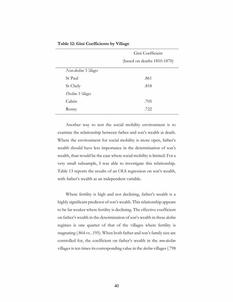
Table 12: Gini Coefficients by Village

Gini Coefficient

(based on deaths 1810-1870)

Non-decline Villages

St Paul .861

St Chely .818

Decline Villages

Cabris .705

Rosny .722

Another way to test the social mobility environment is to

examine the relationship between father and son’s wealth at death.

Where the environment for social mobility is more open, father’s

wealth should have less importance in the determination of son’s

wealth, than would be the case where social mobility is limited. For a

very small subsample, I was able to investigate this relationship.

Table 13 reports the results of an OLS regression on son’s wealth,

with father’s wealth as an independent variable.

Where fertility is high and not declining, father’s wealth is a

highly significant predictor of son’s wealth. This relationship appears

to be far weaker where fertility is declining. The effective coefficient

on father’s wealth in the determination of son’s wealth in these decline

regimes is one quarter of that of the villages where fertility is

stagnating (.864 vs. .195). When both father and son’s family size are

controlled for, the coefficient on father’s wealth in the non-decline

villages is ten times its corresponding value in the decline villages (.798

40

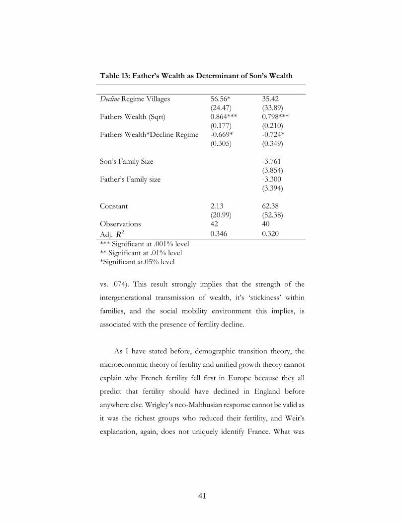
Table 13: Father’s Wealth as Determinant of Son’s Wealth

Decline Regime Villages 56.56*

(24.47) 35.42 (33.89)

Fathers Wealth (Sqrt) 0.864*** (0.177)

0.798*** (0.210)

Fathers Wealth*Decline Regime -0.669* (0.305)

-0.724* (0.349)

Son’s Family Size -3.761

(3.854) Father’s Family size -3.300

(3.394)

Constant 2.13 (20.99)

62.38 (52.38)

Observations 42 40 Adj. 2R 0.346 0.320 *** Significant at .001% level ** Significant at .01% level *Significant at.05% level

vs. .074). This result strongly implies that the strength of the

intergenerational transmission of wealth, it’s ‘stickiness’ within

families, and the social mobility environment this implies, is

associated with the presence of fertility decline.

As I have stated before, demographic transition theory, the

microeconomic theory of fertility and unified growth theory cannot

explain why French fertility fell first in Europe because they all

predict that fertility should have declined in England before

anywhere else. Wrigley’s neo-Malthusian response cannot be valid as

it was the richest groups who reduced their fertility, and Weir’s

explanation, again, does not uniquely identify France. What was

41

unique to France was the pattern of landholding and relative

affluence (to the rest of the world). There are many good reasons to

suspect that social mobility may be a factor behind the decline. The

level of inequality and the perseverance of wealth within families,

both highly related to the social mobility environment were both

found to be negatively associated with the presence of declining

fertility.

Section 6: Conclusion

Through linking the Henry demographic dataset to individual

measures of wealth, the socioeconomic correlates of the fertility

transition have been examined in this paper. The principal result is

the major shift in the wealth fertility relationship at the individual

level. Where fertility is high and non-declining, this relationship is

positive. Where fertility is declining, this relationship is negative. It is

the richest groups who reduce their fertility first. This result

contributes to a revisionist interpretation of the European fertility

decline. In opposition to the EFP’s conclusions, this disaggregated

analysis finds strong socioeconomic correlates for the decline of

fertility in France. The second principal result of this paper is that

spacing strategies, as opposed to stopping strategies, played the

strongest role in achieving a lower family size for the richest groups,

for the villages where fertility was declining. Thirdly, existing theories

on why fertility declined in France failed to be supported by the

empirical data collected. However, a fresh look at an old hypothesis,

does receive some support. Social mobility, as proxied by the level of

42

inequality in the villages and the perseverance of wealth within

families, is strongly associated with fertility decline.

The evidence presented here demonstrates that socioeconomic

status mattered during the early French fertility decline but cannot,

of course, claim to have cracked one of the greatest unsolved puzzles

in economic history. The root causes behind the World’s first fertility

decline are still poorly understood. It is perhaps time to reassess

conceptual models of the fertility transition. Empirically, a

comparative analysis with other European countries based upon

detailed individual level information can hopefully illuminate the

mystery of the early French fertility decline. This study is a first step

towards re-establishing the French experience as paramount in our

understanding of Europe’s demographic transition.

43

References

Archives Départementales de la Alpes-Maritime, serie Q3, Tables Des Successions et Absences.

Archives Départementales de la Dordogne, serie Q3, Tables Des Successions et Absences.

Archives Départementales de la Lozere, serie Q3, Tables Des Successions et Absences.

Archives Départementales de la Seine - St. Denis, serie Q3, Tables Des Successions et Absences.

Becker, Gary S., 1960 ‘An Economic Analysis of Fertility’ in Ainsley J. Coale, ed., Demographic and Economic Change in Developed Countries. Princeton, NJ: Princeton University Press: 209-40

Becker, Gary S. 1991 A treatise on the family. Enlarged ed. Cambridge, MA: Harvard U. Press.

Bengtsson, Tommy and Martin Dribe 2006 “Deliberate control in a natural fertility population: Southern Sweden, 1766–1864” Demography 43(4): 727–746.

Bongaarts, John. 1983. “The proximate determinants of natural marital fertility,” in Rodolfo A. Bulatao and Ronald. D. Lee (eds.), Determinants of Fertility in Developing Countries New York: Academic Press: 103–138.

Bourdieu, Jérôme, Gilles Postel-Vinay and Akiko Suwa-Eisenmann 2004 “Défense et illustration de l’enquête 3000 familles” Annales de démographie historique: 19-52.

Box-Steffensmeier, Janet M., and Bradford S. Jones 2004 Event History Modelling: A Guide for Social Scientists New York: Cambridge University Press

Brown, John C. and Timothy W. Guinnane 2007 “Regions and Time in the European Fertility Transition: Problems in the Princeton Project’s Statistical Methodology” Economic History Review, 60(3): 574-595

Burch, Thomas K. 1995 “Icons, Strawmen and Precision: Reflections on Demographic Theory of Fertility Decline” University of Western Ontario Discussion Paper 94 (4)

Castro, Nina. and Neil J. Cummins 2006 “The Relationship between Socioeconomic Status and Marital Fertility in 18th Century France” Unpublished ICPSR Project

Chesnais, Jean Claude 1992 The Demographic Transition: Stages, Patterns and Economic Implications Oxford: Oxford University Press

44

Coale, Ainsley J. and Susan. C. Watkins 1986 The Decline of Fertility in Europe: The revised proceedings of a conference on the Princeton European Population Project Princeton: Princeton University Press

Clark, Gregory and Gillian Hamilton. 2006 “Survival of the Richest. The Malthusian Mechanism in Pre-Industrial England.” Journal of Economic History, 66(3) (September): 707-36.

Cleves Mario. A., William W. Gould and Roberto G. Gutierrez, 2004 An Introduction to Survival Analysis Using Stata. Revised Edition College Station (TX): Stata Press

Cummins, Neil J. 2009 A Comparative Analysis of the Relationship between Wealth and Fertility during the Demographic Transition: England and France PhD Thesis London School of Economics (forthcoming)

Dumont, Arsene 1890 Dépopulation et civilisation: étude démographique Paris: Lecrosnier et Babé.

Galor, Oded 2004 "From Stagnation to Growth: Unified Growth Theory," CEPR Discussion Papers 4581

Guinnane, Timothy W., Carolyn M. Moehling and Cormac O’Grada 2006 “The fertility of the Irish in the United States in 1910” Explorations in Economic History 43(4): 465-485

Guttmann, Myron P. and Susan C. Watkins 1990 “Socio-Economic Differences in Fertility Control. Is There an Early Warning System at the Village Level?” European Journal of Population 6(1):69-101

Hadeishi, Hajime 2003 “Economic Well-Being and Fertility in France: Nuits, 1744–1792.” Journal of Economic History: 489-505.

Houdaille, Jacques 1984 “La mortalité des enfants dans la France rurale de 1690 a 1779” Population 1: 77-106

Houdaille, Jacques 1976 “Fécondité des mariages dans le quart nord-est de la France de 1670 a 1829” Annales de Demographie Historique: 341-92

Henry, Louis and Jacques Houdaille 1973 “Fécondité des mariages dans le quart nord-ouest” Population (French Edition) 28: 873-924

Henry, Louis 1972 ”Fécondité des mariages dans le quart sud-ouest de la France” Annales E.S.C 27: 612-39, 977-1023

Henry, Louis 1978 “Fecondite des mariages dans le quart sud-est de la France” Population (French Edition) 33: 855-83

Kohler, Hans-Peter, Francesco C. Billari, and José Antonio Ortega 2002 “The emergence of lowest-low fertility in Europe during the 1990s” Population and Development Review 28(4): 641–680

Levy-Leboyer, Maurice and François Bourguignon 1990 A Macroeconomic Model of France during the 19th Century: An Essay in Econometric Analysis Cambridge, Cambridge University Press

Livi-Bacci, Massimo 1986 “Social-group forerunners of fertility control in Europe” in Ansley J. Coale and Susan C. Watkins (eds.) The decline of

45

fertility in Europe Princeton, New Jersey, Princeton University Press: 182-200

Maddison, Angus 2003 The world economy: historical statistics Paris: OECD Murphy, T. and Sandra Gonzalez-Bailón 2008 “When Smaller Families

Look Contagious: A Spatial Look At The French Fertility Decline Using An Agent-Based Simulation Model“ Oxford Discussion Papers in Economic and Social History series 71

Notestein, Frank 1945 “Population; the Long View” in Schultz, Theodore, Food for the World: 36-57

Okun, Barbara 1994 “Evaluating Methods for Detecting Fertility Control: Coale and Trussell's Model and Cohort Parity Analysis” Population Studies 30: 193-222

Piketty, Thomas, Gilles P. Vinay and Jean L. Rosenthal “Wealth concentration in a developing economy : Paris and France, 1807-1994“ American Economic Review 96(1): 236-256

Schmertmann, Carl P. and André J. Caetano 1999 “Estimating Parametric Fertility Models with Open Birth Interval Data” Demographic Research available at http://www.demographic-research.org/Volumes/Vol1/5 (accessed 22 Jan 2008)

Skirbekk, Vergard 2008 “Fertility trends by social status” Demographic Research 18(5): 145-180

Stata Library, Analysing Count Data UCLA: Academic Technology Services, Statistical Consulting Group from http://www.ats.ucla.edu/stat/stata/library/count.htm (accessed 20 January 2008)

Van Bavel, Jan 2002 “Detecting Stopping and Spacing Behavior in Historical Fertility Transitions: A Critical Review of Methods” Working Paper, Department of Sociology, KU Leuven.

Van Bavel, Jan 2004 "Deliberate birth spacing before the fertility transition in Europe: evidence from nineteenth-century Belgium" Population Studies 58(1): 95-107

Van Bavel, Jan & Jan Kok 2004 “Birth spacing in the Netherlands. The effects of family composition, occupation and religion on birth intervals, 1820-1885” European Journal of Population 20(2): 119-140

Van de Walle, Etienne 1978 “Alone in Europe: The French Fertility Decline until 1850” In Historical Studies of Changing Fertility, edited by Charles Tilly, 257–88. Princeton, NJ: Princeton University Press: 257988

Weir, David. R. 1984a “Life Under Pressure: France and England, 1670-1870” Journal of Economic History 44(1) : 27-47

Weir, David. R. 1984b “Fertility Transition in Rural France, 1740-1829” Journal of Economic History 44(2) :612-4

46

Weir, David. R. 1994 “New Estimates of Nuptiality and Marital Fertility in France, 1740-1911” Population Studies, 48(2): 307-331

Weir, David R. 1995 “Family Income, Mortality, and Fertility on the Eve of the Demographic Transition: A Case Study of Rosny-Sous-Bois.” Journal of Economic History 55(1): 1-26

Wrigley, Edward A. 1985 “The Fall of Marital Fertility in Nineteenth-Century France: Exemplar or Exception? (Part I)” European Journal of Population 1(1): 31-60

Xie, Yu and Ellen E. Pimentel 1992 “Age Patterns of Marital Fertility: Revising the Coale-Trussell Method” Journal of the American Statistical Association 87: 977-84

47