mark voorhies 5/5/2017 - university of california, san...
TRANSCRIPT

Heuristic Approaches
Mark Voorhies
5/5/2017
Mark Voorhies Heuristic Approaches

PAM (Dayhoff) and BLOSUM matrices
PAM1 matrix originally calculated from manual alignments ofhighly conserved sequences (myoglobin, cytochrome C, etc.)
We can think of a PAM matrix as evolving a sequence by oneunit of time.
If evolution is uniform over time, then PAM matrices for largerevolutionary steps can be generated by multiplying PAM1 byitself (so, higher numbered PAM matrices represent greaterevolutionary distances).
The BLOSUM matrices were determined from automaticallygenerated ungapped alignments. Higher numbered BLOSUMmatrices correspond to smaller evolutionary distances.BLOSUM62 is the default matrix for BLAST.
Mark Voorhies Heuristic Approaches

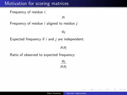
Motivation for scoring matrices
Frequency of residue i :pi
Frequency of residue i aligned to residue j :
qij
Expected frequency if i and j are independent:
pipj
Ratio of observed to expected frequency:
qijpipj
Log odds (LOD) score:
s(i , j) = logqijpipj
Mark Voorhies Heuristic Approaches

Motivation for scoring matrices
Frequency of residue i :pi
Frequency of residue i aligned to residue j :
qij
Expected frequency if i and j are independent:
pipj
Ratio of observed to expected frequency:
qijpipj
Log odds (LOD) score:
s(i , j) = logqijpipj
Mark Voorhies Heuristic Approaches

Motivation for scoring matrices
Frequency of residue i :pi
Frequency of residue i aligned to residue j :
qij
Expected frequency if i and j are independent:
pipj
Ratio of observed to expected frequency:
qijpipj
Log odds (LOD) score:
s(i , j) = logqijpipj
Mark Voorhies Heuristic Approaches
Motivation for scoring matrices
Frequency of residue i :pi
Frequency of residue i aligned to residue j :
qij
Expected frequency if i and j are independent:
pipj
Ratio of observed to expected frequency:
qijpipj
Log odds (LOD) score:
s(i , j) = logqijpipj
Mark Voorhies Heuristic Approaches

Motivation for scoring matrices
Frequency of residue i :pi
Frequency of residue i aligned to residue j :
qij
Expected frequency if i and j are independent:
pipj
Ratio of observed to expected frequency:
qijpipj
Log odds (LOD) score:
s(i , j) = logqijpipj
Mark Voorhies Heuristic Approaches

BLOSUM45 in alphabetical order
Mark Voorhies Heuristic Approaches

Clustering amino acids on log odds scores
import networkx as nxt r y :
import P y c l u s t e rexcept I m p o r t E r r o r :
import Bio . C l u s t e r as P y c l u s t e r
c l a s s S c o r e C l u s t e r :def i n i t ( s e l f , S , a l p h a a a = ”ACDEFGHIKLMNPQRSTVWY” ) :
””” I n i t i a l i z e from numpy a r r a y o f s c a l e d l o g odds s c o r e s . ”””( x , y ) = S . shapea s s e r t ( x == y == l e n ( a l p h a a a ) )
# I n t e r p r e t the l a r g e s t s c o r e as a d i s t a n c e o f z e r oD = max( S . r e s h a p e ( x∗∗2))−S# Maximum−l i n k a g e c l u s t e r i n g , w i th a use r−s u p p l i e d d i s t a n c e mat r i xt r e e = P y c l u s t e r . t r e e c l u s t e r ( d i s t a n c e m a t r i x = D, method = ”m” )
# Use NetworkX to read out the amino−a c i d s i n c l u s t e r e d o r d e rG = nx . DiGraph ( )f o r ( n , i ) i n enumerate ( t r e e ) :
f o r j i n ( i . l e f t , i . r i g h t ) :G . add edge (−(n+1) , j )
s e l f . o r d e r i n g = [ i f o r i i n nx . d f s p r e o r d e r (G, −l e n ( t r e e ) ) i f ( i >= 0 ) ]s e l f . names = ”” . j o i n ( a l p h a a a [ i ] f o r i i n s e l f . o r d e r i n g )s e l f . C = s e l f . permute ( S )
def permute ( s e l f , S ) :””” Given squa r e mat r i x S i n a l p h a b e t i c a l o rde r , r e t u r n rows and columnso f S permuted to match the c l u s t e r e d o r d e r . ”””r e t u r n a r r a y ( [ [ S [ i ] [ j ] f o r j i n s e l f . o r d e r i n g ] f o r i i n s e l f . o r d e r i n g ] )
Mark Voorhies Heuristic Approaches

BLOSUM45 – maximum linkage clustering
Mark Voorhies Heuristic Approaches

BLOSUM62 with BLOSUM45 ordering
Mark Voorhies Heuristic Approaches

BLOSUM80 with BLOSUM45 ordering
Mark Voorhies Heuristic Approaches

Smith-Waterman
The implementation of local alignment is the same as for globalalignment, with a few changes to the rules:
Initialize edges to 0 (no penalty for starting in the middle of asequence)
The maximum score is never less than 0, and no pointer isrecorded unless the score is greater than 0 (note that thisimplies negative scores for gaps and bad matches)
The trace-back starts from the highest score in the matrix andends at a score of 0 (local, rather than global, alignment)
Because the naive implementation is essentially the same, the timeand space requirements are also the same.
Mark Voorhies Heuristic Approaches

Smith-Waterman
A G C G G T A
G
A
G
C
G
GA
0 0 0 0 0 0 0 0
0
0
0
0
0
0
0
0 1 0 0 1 0 0
1 0 0 0 0 0 1
0 2 1 1 1 0 0
0 1 3 2 1 0 0
0 0 2 4 3 2 1
0 1 31 5 4 3
1 0 0 2 4 4 5
Mark Voorhies Heuristic Approaches

Basic Local Alignment Search Tool
Why BLAST?
Fast, heuristic approximation to a full Smith-Waterman localalignment
Developed with a statistical framework to calculate expectednumber of false positive hits.
Heuristics biased towards “biologically relevant” hits.
Mark Voorhies Heuristic Approaches

BLAST: A quick overview
Mark Voorhies Heuristic Approaches

BLAST: Seed from exact word hits
Mark Voorhies Heuristic Approaches

BLAST: Myers and Miller local alignment around seed pairs
Mark Voorhies Heuristic Approaches

BLAST: High Scoring Pairs (HSPs)
Mark Voorhies Heuristic Approaches

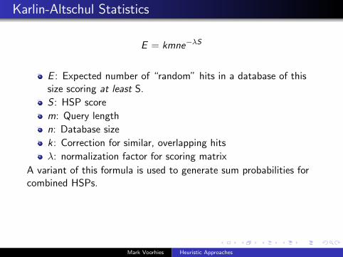
Karlin-Altschul Statistics
E = kmne−λS
E : Expected number of “random” hits in a database of thissize scoring at least S.
S : HSP score
m: Query length
n: Database size
k: Correction for similar, overlapping hits
λ: normalization factor for scoring matrix
A variant of this formula is used to generate sum probabilities forcombined HSPs.
p = 1− e−E
(If you care about the difference between E and p, you’re alreadyin trouble)
Mark Voorhies Heuristic Approaches

0th order Markov Model
Mark Voorhies Heuristic Approaches

1st order Markov Model
Mark Voorhies Heuristic Approaches

1st order Markov Model
Mark Voorhies Heuristic Approaches

1st order Markov Model
Mark Voorhies Heuristic Approaches

What are Markov Models good for?
Background sequence composition
Spam
Mark Voorhies Heuristic Approaches

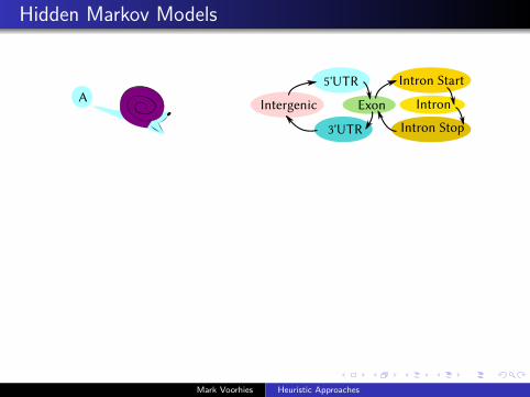
Hidden Markov Models
Mark Voorhies Heuristic Approaches
Hidden Markov Models
Mark Voorhies Heuristic Approaches

Hidden Markov Models
Mark Voorhies Heuristic Approaches

Hidden Markov Models
Mark Voorhies Heuristic Approaches

Hidden Markov Models
Mark Voorhies Heuristic Approaches

Hidden Markov Model
Mark Voorhies Heuristic Approaches

The Viterbi algorithm: Alignment
Mark Voorhies Heuristic Approaches

The Viterbi algorithm: Alignment
Dynamic programming, likeSmith-Waterman
Sums best log probabilitiesof emissions and transitions(i.e., multiplyingindependent probabilities)
Result is most likelyannotation of the targetwith hidden states
Mark Voorhies Heuristic Approaches

The Forward algorithm: Net probability
Probability-weighted sumover all possible paths
Simple modification ofViterbi (although summingprobabilities means we haveto be more careful aboutrounding error)
Result is the probability thatthe observed sequence isexplained by the model
In practice, this probabilityis compared to that of a nullmodel (e.g., randomgenomic sequence)
Mark Voorhies Heuristic Approaches

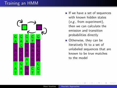
Training an HMM
If we have a set of sequenceswith known hidden states(e.g., from experiment),then we can calculate theemission and transitionprobabilities directly
Otherwise, they can beiteratively fit to a set ofunlabeled sequences that areknown to be true matchesto the model
The most common fittingprocedure is theBaum-Welch algorithm, aspecial case of expectationmaximization (EM)
Mark Voorhies Heuristic Approaches

Profile Alignments: Plan 7
(Image from Sean Eddy, PLoS Comp. Biol. 4:e1000069)
Mark Voorhies Heuristic Approaches

Profile Alignments: Plan 7 (from Outer Space)
(Image from Sean Eddy, PLoS Comp. Biol. 4:e1000069)
Mark Voorhies Heuristic Approaches

Rigging Plan 7 for Multi-Hit Alignment
(Image from Sean Eddy, PLoS Comp. Biol. 4:e1000069)
Mark Voorhies Heuristic Approaches

HMMer3 speeds
Eddy, PLoS Comp. Biol. 7:e1002195
Mark Voorhies Heuristic Approaches

HMMer3 sensitivity and specificity
Eddy, PLoS Comp. Biol. 7:e1002195
Mark Voorhies Heuristic Approaches

Stochastic Context Free Grammars
Can emit from both sides → base pairs
Can duplicate emitter → bifurcations
Mark Voorhies Heuristic Approaches

INFERNAL/Rfam
Modified from the INFERNAL User Guide – Nawrocki, Kolbe, and Eddy
Mark Voorhies Heuristic Approaches

INFERNAL/Rfam
Modified from the INFERNAL User Guide – Nawrocki, Kolbe, and Eddy
Mark Voorhies Heuristic Approaches

INFERNAL/Rfam
Modified from the INFERNAL User Guide – Nawrocki, Kolbe, and Eddy
Mark Voorhies Heuristic Approaches

INFERNAL/Rfam
Modified from the INFERNAL User Guide – Nawrocki, Kolbe, and Eddy
Mark Voorhies Heuristic Approaches

INFERNAL/Rfam
Modified from the INFERNAL User Guide – Nawrocki, Kolbe, and Eddy
Mark Voorhies Heuristic Approaches

INFERNAL/Rfam
Modified from the INFERNAL User Guide – Nawrocki, Kolbe, and Eddy
Mark Voorhies Heuristic Approaches

INFERNAL/Rfam
Modified from the INFERNAL User Guide – Nawrocki, Kolbe, and Eddy
Mark Voorhies Heuristic Approaches

Homework
Keep working on your dynamic programming code.
Mark Voorhies Heuristic Approaches