Market Access and Regional Specialization in a Ricardian World

A. Kerem CosarU. of Chicago Booth

Pablo D. FajgelbaumUCLA

October 2012

Abstract

When trade is costly within countries, international trade leads to concentration of eco-

nomic activity in locations with good access to foreign markets. Costly trade within countries

also makes it harder for remote locations to gain from international trade. We investigate the

role of these forces in shaping industry location, employment concentration and the gains from

international trade. We develop a model that features Ricardian comparative advantages be-

tween countries, coupled with di¤erences in proximity to international markets across locations

within a country. In the model, international trade creates a partition between a coastal and

an interior region that di¤er in population density and specialization patterns. We assess the

model prediction for industry location across U.S. counties. In tune with the theory, we �nd

that U.S. export-oriented industries are more likely to locate and to employ more workers closer

to international ports. We use the model to measure the importance of international trade

in concentrating economic activity, and of domestic trade costs in hampering the gains from

international trade.

1 Introduction

International trade is an important determinant of the geographic distribution of economic

activity within countries. In China, the export growth of the past few decades occurred jointly

with movements of rural workers and export oriented industries toward coastal regions (World

Bank, 2009). After the U.S.-Vietnamese trade agreement, employment expanded in Vietnamese

comparative-advantage industries located closer to major seaports (McCaig and Pavnick, 2012).

In Mexico, increased trade with the U.S. led to larger manufacturing employment near the U.S.

border (Hanson, 1996). It is also well known that the distribution of employment is skewed towards

coasts: half of the world population lives within 100 kilometers of coastlines or navigable rivers,

while 19 out of the 25 largest cities in the world are coastal.1 While the appeal of coastal sites

derives in part from their resources and amenities, a reason for their primacy is that they are well

suited for trading with other countries.

These examples showcase the impact of international trade on the regional distribution of eco-

nomic outcomes. At the same time, they highlight the relevance of costly trade within countries.

The larger the domestic trade costs, the stronger the incentives for export oriented industries to

concentrate in places with good access to international markets, and the harder for remote locations

to gain from trade. In this paper, we investigate the role of these forces in shaping the location

of industries, the concentration of employment, and the gains from international trade. For that,

we develop a theory of international trade with costly trade within countries, and we assess its key

empirical and quantitative implications.

Our approach features Ricardian comparative advantages across countries coupled with di¤er-

ences in international market access across locations within a country. We �rst lay out a baseline

model, and we use it to characterize how international and domestic trade costs determine industry

location, employment concentration and the gains from trade. The model is highly tractable, and

it o¤ers analytic solutions for all our key outcome variables. Then, we apply the theory to the

U.S. economy. In tune with the theory, we �nd that U.S. export-oriented industries are more likely

to locate and employ more workers closer to international gates such as ports or land crossings.

Finally, we use the model to establish the quantitative relevance of international trade for the

concentration of economic activity, and to measure by how much domestic trade costs hamper the

gains from international trade.

In the theory, we furnish the canonical model of international trade driven by Ricardian com-

parative advantages with a geography within countries. Locations within a country are arbitrarily

arranged in a map and di¤er in distance to an international gate such as a seaport, an airport

or a land crossing into another country. Within the country trade is costly, and international

shipments must cross through the international gate. To produce, each location uses a perfectly

mobile resource (workers) and an immobile resource (land). Congestion forces are represented by

decreasing returns to labor, so that it is not optimal to concentrate production in a single location.

1Authors�calculation from Harvard CID. The reported number is for 1995.

2

Relative productivity across industries is the same in all locations within a country, but di¤ers

between countries. International di¤erences in institutions, recently emphasized as an important

determinant of trade and specialization, exemplify a source of comparative advantage that does not

vary systematically across locations within countries.

We use the model to study how international and domestic trade costs interact to determine

regional patterns of production and employment. We �nd that whenever an open economy is not

fully specialized in what it exports, two distinct regions necessarily emerge. The equilibrium fea-

tures a region with high population density near the international gate that specializes in producing

export-oriented goods, followed by a region with low population density that is incompletely spe-

cialized and does not trade with the rest of the world. Thus, even though trade costs are uniform

across space, international trade generates a partition between a "coastal" and an "interior" re-

gion. The boundary between these regions, as well as their shares in employment and output, is

endogenous and depends on international and domestic trade costs.

We analyze how changes in trade costs interact with factor movements within the country and

with the gains from trade. Reductions in international or domestic trade costs lead to migration of

mobile factors toward the locations with good international market access. Lower trade costs also

cause the boundary between the coastal and the interior regions to move inland, so that marginal

locations switch from autarky to trading with the rest of the world, and the geographic extension of

the integrated region increases. As a result, employment density and the share in national income

rises in the coastal region relative to the interior region.

We conclude the theoretical analysis by investigating the impact of domestic trade costs on

the gains from international trade. Aggregate welfare and real income can be decomposed into a

familiar term that captures the gains from trade without domestic geography, and a new term that

captures the e¤ect of domestic trade frictions. The �rst component depends on the terms of trade,

as in a standard Ricardian model, and on congestion forces. The second component depends on

domestic trade costs, and on the size of the trading region in terms of employment and land use.

Since larger domestic frictions cause the trading region to shrink, the gains from international trade

decrease with domestic trade costs.

We apply our theory to the U.S. economy. Since in the U.S. domestic trade costs are relatively

small, applying the theory in this context represents a useful benchmark. We start by assessing

the implications of the model for the location of industries. The key ingredients from the theory,

di¤erences in international market access and Ricardian comparative advantages, cause industries

to arrange in space based on their export orientation at the national level. This suggests a way

of detecting an e¤ect of international market access on regional specialization: export-oriented

industries should be more likely than import-competing ones to locate, and to employ more work-

ers, closer to international gates such as seaports, international airports or land crossings. This

explanation for industry location complements common explanations given the literature, such as

natural advantages or agglomeration.2

2See Holmes and Stevens (2004) for a summary assessment of the forces determining industry location in the U.S.

3

We use U.S. data on specialization at the county and national levels to investigate this pre-

diction. We classify industries as either export-oriented or import-competing at the national level,

and we also rank these industries by the strength of their revealed comparative advantages. Then,

we use county-level employment data to investigate how employment varies within each industry

across districts based on the industry export orientation and on the county distance to interna-

tional gates. We �nd support for the prediction that export-oriented industries, or industries with

stronger revealed comparative advantages, are relatively more likely to locate closer to international

gates such as seaports, land-crossings or airports. Moving inland from a representative port for

400 miles, a value close to the 90th percentile of the distribution of county distances to the nearest

port, employment in export-oriented industries relative to import-competing industries shrinks by

between 18% and 44%, depending on the speci�cation.

Finally, we propose a simple quantitative methodology for measuring the e¤ects of the theory

on the concentration of employment and the gains from trade. According to Rappaport and Sachs

(2003), U.S. coastal counties collectively account for 13% of continental US land area and for 51% of

its 2000 population. In our model, international trade is the only source of dispersion in economic

activity across locations, and it generates an endogenous partition between coastal and interior

regions. Therefore, we ask, How important is international trade for the concentration of activity

in coastal areas?

Second, we measure the impact of domestic trade costs on the gains from international trade. A

recent literature emphasizes that the gains from international trade are relatively small.3 Needless

to say, understanding the forces that determine the gains from trade is important to inform both

theory and policy. Therefore, we ask, How important are domestic trade costs in hampering the

gains from international trade?

The answer to these questions depends on some key parameters of the model: domestic trade

costs, decreasing returns to scale, international comparative advantages, and sectorial consumption

shares. First, we obtain these parameters matching features of the data that are independent from

the geographic distribution of employment. As natural targets for the key parameters we use the

share of shipping costs in export-oriented shipments, the share of land in sectorial income, trade

intensity at the country level, and household expenditure shares. Then, we use the calibrated model

to predict the population density in the coastal relative to the interior region, and to measure the

gains from trade for di¤erent levels of domestic trade costs.

Depending on our de�nition of coastal districts in the data, we �nd that Ricardian comparative

advantages explain close to 1=3 of the concentration of activity in coastal districts in the U.S.

relative to interior districts. The part left unexplained by the model is naturally attributable to

forces that we do not consider, such as amenities, factor endowments or agglomeration. Finally,

we measure the gains from international trade in the U.S. to be in the order 0:4%. At the same

time, keeping all other parameters the same, if the magnitude of domestic trade costs in the model

3For example, Arkolakis et al. (2011) show that a certain class of trade models predicts that the share of realincome that the U.S. would loose if access to international trade were shut down is around 1%.

4

shrink by 50% these gains rise to 0:7%, while if domestic trade costs are suppressed they rise to

4:2%.

These results on population density and gains from trade hold even though, as pointed out by

others, domestic trade costs in the U.S. are quite small. In our calibration, they represent 1:5%

of the f.o.b price of exported products. Given that the baseline model does not include a number

of additional forces, the large e¤ect on the gains from trade is likely an upper bound for the e¤ect

of domestic frictions.4 Still, this large potential e¤ect of small domestic costs suggests that local

trade frictions might play an even more important role in poor countries, where infrastructure is

presumably underdeveloped relative to the U.S..

Relation to the Literature A vast literature is concerned with studying the concentration of

economic activity in contexts with agglomeration. However, few papers in that literature consider

an interaction between international and domestic trade costs. In a context with demand linkages,

Krugman and Livas-Elizondo (1996) and Behrens et al. (2006) present models where two regions

within a country trade with the rest of the world. Henderson (1982) and Rauch (1991) embed

system of cities models in open economy frameworks.5 Rossi-Hansberg (2004) studies the location

of industries that di¤er in relative productivity on a continuous space with externalities. All these

papers are based on an agglomeration force to induce concentration. In contrast, in our context,

concentration results exclusively from the interaction between heterogeneous market access within

countries and comparative advantages between countries. We focus on these forces in our empirical

and quantitative applications.

Closer to a neoclassical environment, Bond (1993) and Courant and Deardor¤ (1993) present

models with regional specialization where relative factor endowments may vary across discrete

regions within a country. These papers do not include heterogeneity in access to world markets.

Venables and Limao (2002) study geographic specialization across regions trading with a central

location but do not allow for factor mobility. More recently, Ramondo et al. (2011) study the gains

from trade and ideas di¤usion allowing for multiple regions within countries, but do not focus their

analysis on di¤erences in world market access across locations or on labor mobility within countries.

Redding (2012) extends the framework in Eaton and Kortum (2002) with labor mobility within a

country to study regional gains from trade. In his analysis, for each good there are independent

productivity draws across locations. We assume that locations share access to the same technologies

within a country, so that industries choose their location based on comparative advantages at the

national level and on distance to international gates.

4 In Section 5 of the paper, we lay out an extended model that adds additional forces not considered in the baselinecalibration. In the extended model, we consider industry-speci�c congestion forces and consumption of housing andservices. In ongoing work, we are developing a calibration of the extended model.

5We share with Rauch (1991) the presence of Ricardian comparative advantages with internal geography. Incontrast with that paper, we ask a di¤erent set of questions, we assess both empirical and quantitative implicationsof the theory, and we present a neoclassical model that is specially tractable to characterize the distribution ofpopulation and to illustrate the answer to our main questions.

5

Structure of the Paper We start in Section 2 by laying out the baseline model, characterizing

the general equilibrium and presenting the comparative statics of population density and welfare

with respect to domestic trade costs. In Section 3 we assess the model prediction for regional

specialization with U.S. data, and in section 4 we present the quantitative assessment. In Section

5 we develop an extended model.6 Section 6 concludes. Proofs are in the appendix.

2 Baseline Model

Geography and Trade Costs A country consists of a set of locations arbitrarily arranged on

a map. We index locations by `, and we assume that only location ` = 0 can trade with the rest

of the world. That is, a good can be shipped internationally from a location ` only if it crosses

through location ` = 0.

As it will be clear later on, given the nature of our model only the distance at which each

location ` lies from location 0 matters for the equilibrium. Therefore, we assume without loss of

generality that ` represents the distance separating locations ` and 0. We also let ` represent the

location at maximum distance from ` = 0.

There are two industries, i 2 fX;Mg. International and domestic trade costs are industryspeci�c. The international iceberg cost in industry i between ` = 0 and the rest of the world (RoW)

is e�i0 . Within the country, iceberg trade costs are constant per unit of distance. Therefore, the

cost of shipping a good for distance d in industry i equals e�i1d. This implies a cost of international

trade equal to e�i0+�

i1` in industry i from location `.

Given this geography, we can interpret ` = 0 as a port, the set locations surrounding it as a

coast, and the rest of the country as an interior. In the equilibrium of the model, there will be a

formal sense in which locations endogenously belong to a coastal or to an interior region.

More generally, we can think of ` = 0 as the point in space with the best access to international

markets. What is key is that not all locations have the same technology for trading with the RoW.

This will drive concentration near points with goods access. Internal geography vanishes when

� i1 = 0 for both industries.7

Endowments There are two factors of production, a perfectly mobile factor and a �xed factor.

We refer to the mobile factor as workers, and to the �xed factor as land. More generally, the �xed

factor could account for immobile workers, or for structures that take long to depreciate.

We choose units such that the national land endowment equals 1, and we let � (`) be the amount

of land available in each location `. Land is owned by immobile landlords who do not work and

who spend their rental income locally.

6We are currently working on the calibration of the extended model.7Our analysis equivalently applies to an arbitrary number of ports, as long as all ports face the same relative

prices in the rest of the world. In that case, we would let ` index the distance to the nearest port. If ports di¤ered inthe international prices that they face, the analysis would be heavier in notation but all the key results would carrythrough.

6

We let n be the total number of workers, equal to the labor to land ratio at the national level.

These workers are mobile across locations `. We let n (`) denote employment density at location `,

which is to be determined in equilibrium.

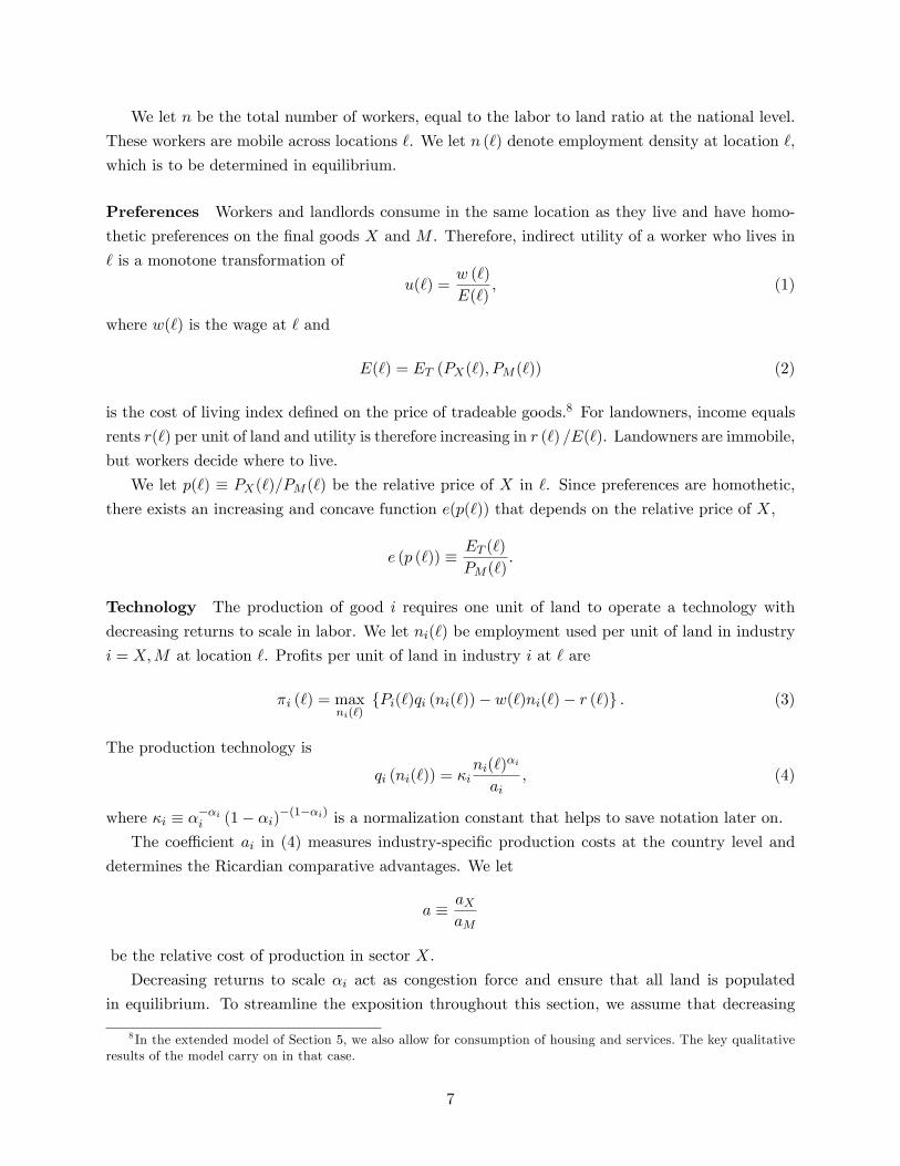
Preferences Workers and landlords consume in the same location as they live and have homo-

thetic preferences on the �nal goods X and M . Therefore, indirect utility of a worker who lives in

` is a monotone transformation of

u(`) =w (`)

E(`); (1)

where w(`) is the wage at ` and

E(`) = ET (PX(`); PM (`)) (2)

is the cost of living index de�ned on the price of tradeable goods.8 For landowners, income equals

rents r(`) per unit of land and utility is therefore increasing in r (`) =E(`). Landowners are immobile,

but workers decide where to live.

We let p(`) � PX(`)=PM (`) be the relative price of X in `. Since preferences are homothetic,

there exists an increasing and concave function e(p(`)) that depends on the relative price of X,

e (p (`)) � ET (`)

PM (`).

Technology The production of good i requires one unit of land to operate a technology with

decreasing returns to scale in labor. We let ni(`) be employment used per unit of land in industry

i = X;M at location `. Pro�ts per unit of land in industry i at ` are

�i (`) = maxni(`)

fPi(`)qi (ni(`))� w(`)ni(`)� r (`)g . (3)

The production technology is

qi (ni(`)) = �ini(`)

�i

ai, (4)

where �i � ���ii (1� �i)�(1��i) is a normalization constant that helps to save notation later on.The coe¢ cient ai in (4) measures industry-speci�c production costs at the country level and

determines the Ricardian comparative advantages. We let

a � aXaM

be the relative cost of production in sector X.

Decreasing returns to scale �i act as congestion force and ensure that all land is populated

in equilibrium. To streamline the exposition throughout this section, we assume that decreasing

8 In the extended model of Section 5, we also allow for consumption of housing and services. The key qualitativeresults of the model carry on in that case.

7

returns are the same in both industries: �X = �M = � .9

The local pattern of specialization at ` is captured by the amount of land �i(`) � �(`) used inby each industry i = X;M .

2.1 Local Equilibrium

We de�ne can characterize a local equilibrium at each location ` that takes prices fPX (`) ; PM (`)gand the real wage u� as given.

De�nition 1 (Local Equilibrium) A local equilibrium at ` consists of employment density n (`),labor demands fni (`)gi=X;M , specialization patterns f�i (`)gi=X;M , and factor prices fw (`) ; r(`)gsuch that

1. workers maximize utility,w (`)

E (`)� u�; = if n (`) > 0; (5)

2. pro�ts are maximized,

�i (`) � 0; = if �i (`) > 0, for i = X;M; (6)

where �i (`) is given by (3);

3. land and labor markets clear, Xi=X;M

�i(`) = �(`); (7)

Xi=X;M

�i(`)

�(`)ni(`) = n (`) ; and (8)

4. trade is balanced.

Conditions 2 to 4 resemble a small Ricardian economy that takes prices as given. In addition,

in each local economy ` the employment density n (`) is determined by (5).

We let pA be the autarky price in location `. By this, we mean the price prevailing in the

absence of trade with any other location or with the rest of the world, but when labor mobility is

allowed. Since in autarky both goods must be produced, condition (6) implies

pA = a. (9)

The specialization pattern can be readily characterized based on relative prices. Using (6),

location `must be fully specialized inX when p (`) > pA, and fully specialized inM when p (`) < pA.

9 In the extended model of Section 5 we allow for di¤erences in �i across industries.

8

The main implication is that a trading location is (generically) fully specialized. When a location

trades, with either the rest of the world or with other locations, it takes relative price p (`) as given.

Unless the relative price p (`) coincides with pA, the location will be fully specialized in one of the

two industries. When p (`) coincides with pA, the location might either export or stay in autarky.

This logic also implies that an incompletely specialized location is (generically) in autarky.10

The solution to the �rm�s problem yields labor demand per unit of land used by industry i,

ni(`) =�

1� �

�Pi(`)

aiw(`)

�1=(1��)(10)

for i = X;M and ` 2�0; `�. To solve for the wage w(`) we note that whenever a location is

populated, the local labor supply decision (5) must be binding:

w(`) = E(`) � u�. (11)

Expressions (10) and (11) convey the various forces that determine the location decision of

workers. Agents care about the e¤ect of prices on both their income and on their cost of living.

Our assumptions guarantee that agents employed in an industry-location pair (i; `) enjoy a higher

real income when the local relative price of industry i is higher in location `. That is, the income

e¤ect from a higher relative price necessarily o¤sets any cost-of-living e¤ect.11 At the same time

there are congestion forces, so that everything else equal agents prefer to avoid places with high

employment density.

Using (9) and (10) we see that if p (`) = pA then employment density is the same across sectors,

nX(`) = nM (`). Therefore, using the market clearing conditions (7) and (8), employment density

n(`) in location ` is

n(`) =

(nX(`)

nM (`)ifp (`) � pAp (`) < pA

. (12)

When p (`) 6= pA, locations are fully specialized and necessarily export. In this circumstance

n(`) increases with the relative price of the exported good. Also, regardless of whether a location

trades or is in autarky, an increase in the national real wage u� keeping relative prices constant

causes workers to emigrate from `.

We summarize the properties of local equilibrium as follows.

Proposition 1 (Local Equilibrium) Let pA be the autarky price in location `. Then: (i) location` is fully specialized in X when p (`) > pA, and fully specialized in M when p (`) < pA; (ii) if

p (`) 6= pA, population density n(`) is increasing in the relative price of the exported good; and (iii)population density n(`) is decreasing in the real wage u�.

10This also holds in the more general case of section 5 where �i di¤ers across sectors. In that case, pA must bedetermined endogenously, but the specialization pattern is still independent from � (`).

11For this note that PX(`)=E(`) = p (`) =e (p (`)) is increasing in the relative price of X, while PM (`)=E(`) =1=e (p (`)) is decreasing in p (`).

9

2.2 General Equilibrium

We have characterized the local equilibrium independently from a location�s geographic position.

We move on to study how market access matters for the employment density and the specialization

pattern in general equilibrium. We study a small economy that takes international prices fP �X ; P �Mgas given. We let

p� =P �XP �M

be the relative price at RoW, and we let

� j �1

2

Xi=X;M

� ij for j = 0; 1

be the average international and domestic iceberg cost across sectors.

No arbitrage implies that for any pair of locations prices satisfy

Pi(`0)=Pi(`) � e�

i1j`�`0j for i = X;M , `; `0 2

�0; `�. (13)

This condition binds if a good in industry i is shipped from ` to `0. A similar condition holds with

respect to RoW. In particular, since location ` = 0 can trade directly with RoW, (13) implies

e�2�0 � p(0)=p� � e2�0 . (14)

The �rst inequality is binding if the country exports X to RoW, while the second is if it imports

X. In turn, for any location ` we have

e�2�1` � p(`)=p(0) � e2�1`, (15)

where the �rst inequality binds if ` exports X to RoW, and second does if ` imports X.

We are ready to de�ne the general equilibrium of the economy.

De�nition 2 (General Equilibrium) An equilibrium in a small economy given international

prices fP �X ; P �Mg consists of a real wage u�, local outcomesnfni (`) ; �i (`)gi=X;M ; n (`) ; w (`) ; r(`)

oand goods prices fPi(`)gi=X;M such that

1. given fPi(`)gi=X;M and u�, the local outcomesnfni (`) ; �i (`)gi=X;M ; n (`) ; w (`) ; r(`)

ocon-

stitute a local equilibrium by De�nition 1 for all ` 2�0; `�;

2. the real wage u� adjusts such that the national labor market clears,

Z `

0n (`)� (`) d` = n; and (16)

3. relative prices p(`) satisfy the no-arbitrage conditions (14) and (15) for all ` 2�0; `�.

10

Since De�nition 1 of a local equilibrium includes trade balance for each location, trade must

also balance at the national level.

We show next that the no-arbitrage conditions restrict the set of trade �ows that can arise in

equilibrium. This feature of the equilibrium is important to characterize regional specialization

patterns.

Lemma 1 There are no bilateral trade �ows between any pair of locations within the country.Hence, the country is in international autarky if and only if all locations in the country are in

autarky and incompletely specialized.

This result is a type of spatial impossibility theorem, in the tradition of Starrett (1978). Since

all locations share the same relative unit costs, there are no gains from trade within the country.

With this in mind we can characterize the general equilibrium. We can partition locations into

the set of those that trade with RoW and those that stay in autarky. If the country exports X,

then all locations that trade with RoW must also export X. It follows that all locations ` such that

e�2(�0+�1`)p� < pA must stay in autarky, for if they specialized in X then, given the specialization

pattern from Proposition 1, the resulting price p (`) = e�2(�0+�1`)p� would induce specialization in

Y . In the same way, all locations ` such that e�2(�0+�1`)p� > pA must specialize in X, for if they

stayed in autarky, the equilibrium price p (`) = pA would violate the no-arbitrage condition (15).

We conclude that the distance to ` = 0 is the only fundamental di¤erence across locations. This

justi�es our previous statement that locations may be arbitrarily arranged on a map, as well as our

initial choice of indexing them by their distance to the port.

Hence, if the country is not in international autarky there is some boundary b 2�0; `�such

that all locations ` < b are fully specialized in the export industry. In turn, all locations ` > b do

not trade with the RoW and stay in autarky. Hence, the internal boundary b divides the country

between a trading "coastal region" comprising all locations ` 2 [0; b] close to the international gate,and an autarkic "interior region" comprising all locations ` 2 (b; `].

Since all locations ` 2 (b; `] are in autarky, they are incompletely specialized and their relativeprice is pA = a. Given this price in the autarkic region and the regional pattern of production, the

no-arbitrage conditions (14) and (15) give the price distribution:

p(`) =

8<:p�e�2(�0+�1min[`;b]) if the country is net exporter of X;p�e2(�0+�1min[`;b]) if the country is net exporter of M:(17)

Using this relative price function we can describe the distribution of employment across loca-

tions. From now on we assume that a < p�, so that the economy has comparative advantages in

sector X. As shown below this implies that, if the economy exports, it must export X. In this case

the employment density depends on location as follows:

n(`) =�

1� �

�p(`)=e(p(`))

aX � u�

�1=(1��)for ` 2

�0; `�. (18)

11

Employment density is governed by relative prices. When the country trades with RoW, the relative

price of the export industry decreases toward the interior, so that employment also decreases as we

move away from the port. Therefore, international and domestic trade costs a¤ect the distribution

of employment across locations through their impact on the relative price gradient in (17).

Using (18) in the aggregate labor-market clearing condition (16) we solve for the real wage as

function the boundary b:

u� =1

aX

��= (1� �)

n

�1�� Z b

0

�p(`)

e(p(`))

� 11��

� (`) d`+

�p(b)

e(p(b))

� 11��

Z `

b� (`) d`

!1��. (19)

In turn, continuity of the relative function determines the location of the boundary b,

p(b) � pA, = if b < `. (20)

We note that, when p(`) > pA, then b = ` and the interior region does not exist. The general

equilibrium is fully characterized by the pair fu�; bg that solves (19) and (20). From the second

equation we �nd a unique value for b, and using that value in (19) we determine the real wage. All

other variables easily follow from these two outcomes.

For future reference we now de�ne the average population density in the coastal region,

nC =

Z b

0n (`)

� (`)R b0 � (`) d`

d`, (21)

while nA � n (b) is average population density in the autarkic interior region.We summarize our �ndings so far as follows.

Proposition 2 (Population and Industry Location in General Equilibrium) Given the in-ternational relative price p�, there is a unique small-country equilibrium, where: (i) in international

autarky, the distribution of prices, wages and labor is uniform across locations; (ii) if the country

trades, employment density increases toward the coast; and (iii) if the country trades and is not

fully specialized, there exists an interior region (b; `] that is in autarky and incompletely specialized,

and a coastal region [0; b] with higher population density that trades with RoW and specializes in

the export-oriented industry.

These results demonstrate that international trade drives concentration of economic activity

and industry location. In the absence of international trade, there are no di¤erences in economic

outcomes across locations. In contrast, when the economy trades, population increases towards

international gates. Furthermore, when the economy trades but is not fully specialized, two dis-

crete regions emerge: a coastal region surrounding international gates that is densely populated,

connected to international markets and specialized in the export-oriented industry; and an interior

region that is lowly populated, disconnected from the rest of the world and incompletely specialized.

12

In our reasoning so far we have assumed a given trade pattern at the national level. Next, we

establish the conditions on the parameters that determine the national trade pattern and existence

of the interior region.

Proposition 3 (National Trade Pattern and Existence of Interior Region) (i) The coun-try exports X if pA=p� < e�2�0; in that case, the interior region exists if and only if e�2(�0+�1`) <

pA=p�; (ii) the country exports M if e2�0 < pA=p

�; in that case, the interior region exists if and

only if pA=p� < e2(�0+�1`); and (iii) the country is in international autarky if e�2�0 < pA=p� < e2�0.

The �rst implication of these results is that domestic trade costs��X1 ; �

M1

, while capable of

a¤ecting the gains and the volume of international trade, can not a¤ect the pattern or the existence

of it. In other words, the conditions that determine when international trade exists as well as the

direction of international trade �ows are the same as in an environment without domestic geography.

The second implication is that, when then country trades, there is an interior region when trade

cost f�1; �0g or the extension of land ` are su¢ ciently large, or when comparative advantages,captured by pA=p�, are not su¢ ciently strong.

2.3 Impact of Changes in International and Domestic Trade Costs

We use the model to characterize the impact of international and domestic trade costs on the

concentration of economic activity and the gains from trade. In the quantitative section we measure

the importance of these e¤ects.

Our motivating examples from the introduction show that international trade integration is

associated with shifts in economic concentration. In our model, population density varies across

locations based on the proximity to the international gate, and population density in the coastal

region relative to the interior region is endogenous. We summarize the impact of trade costs on

these outcomes as follows.

Proposition 4 (Internal Migration) Consider an initial equilibrium where the boundary is at

b 2�0; `�. Then, a reduction in international or in domestic trade costs causes b to move inland,

a net population increase in the coastal region [0; b], and an increase in the relative coastal density

nC=nA.

The direct impact of a reduction in trade costs is that the relative price of the exported industry

increases in the coastal region. In the case of a reduction in �0, the shift is uniform across locations,

while a lower �1 results in a �attening of the slope of relative prices toward the interior. In both

cases, the change in prices causes the relative price at b to be larger than the autarky price pA,

so that locations at the boundary now �nd it pro�table to specialize in export industries and the

boundary moves inland.

What are the internal migration patterns associated with these reductions in trade costs? As

we show below, a consequence of lower trade costs is an increase in the real wage u�. Since in the

13

interior relative prices remain constant, this causes labor demand to shrink. As a result, workers

migrate away from interior locations toward the coast, and relative population density increases in

the coastal region.

These results reproduce the cases that we highlight in the introduction: as trade costs decline,

employment migrates to coastal areas that host comparative-advantage industries. In the quantita-

tive section, we compare the model-generated and empirical values for the relative coastal density

nC=nA to measure the relevance international and domestic trade costs on employment concentra-

tion in the U.S.

We conclude with the impact of domestic trade costs �1 on the gains from international trade.

We �rst de�ne the real wage in the absence of domestic trade costs in an economy that faces relative

prices equal to p:

u (p) � p=e (p)aX

�1� ��

n

���1. (22)

As in a standard Ricardian model, the real wage is increasing in the terms of trade. In addition,

as long as � < 1, it decreases with the number of workers. In our economy with positive trade

costs, the real wage that would prevail in each local economy ` if the national economy was in

international autarky is ua � u (pA). Using the solution for the real wage u� from (19) together

with (22), we can express the gains from international trade when �1 > 0 as follows:12

u�

ua=

Z b

0

�u (p (`))

ua

�1=(1��)� (`) d`+

Z `

b� (`) d`

!1��.

The aggregate gains of moving from autarky to free trade, u�=ua, are a weighted average

of the gains from international trade faced by each local economy, u (p (`)) =ua. The weights

across locations are given their land shares, � (`). Since in interior locations ` 2 [0; b] we haveu (p (`)) =u (pA) = 1, the gains from trade are increasing with the equilibrium position of the

boundary b.

It follows that the larger the size of the export-oriented region, the more a country bene�ts

from openness. Since �1 causes the export oriented region to shrink, the lower the domestic trade

costs, the more we should expect the country to bene�t from openness. A lower �1 makes exporting

pro�table for locations further away from the port, allowing economic activity to spread out and

mitigate the congestion forces in dense coastal areas.

To formalize these results, we de�ne the elasticity of the consumer price index,

"(p) =de(p)=e (p)

dp=p.

12There are two factors of production in this model. For the perfectly mobile factor (labor), the real income u� isequalized across locations, while for the �xed factor (land), the real return r (`) =E (`) depends on location. In whatfollows, we focus our analysis on u. However, our production technology implies that the average real return to land,R `0(r (`) =E (`))� (`) d`, is proportional to u�. Therefore, our statements about the real wage also apply to aggregate

welfare and to aggregate income de�ated at local prices.

14

We also de�ne the share of location ` in total employment,

s (`) =n (`)� (`)

n.

Using these de�nitions, we have the following.

Proposition 5 (Gains from International Trade) The change in the real wage due to changesin p�, �0 or �1 is cu� = Z b

0[1� "(p(`))] s (`) dp(`)

p(`)d`: (23)

Therefore: (i) the change in the real wage caused by terms of trade improvement of bp is boundedabove by the employment share in export-oriented locations,

cu�bp <

Z b

0s (`) d`;

and (ii) domestic trade costs �1 reduce the gains from trade,

d(u�=ua)

d�1< 0.

Expression (23) describes the gains from a reduction in trade costs, either domestic or interna-

tional, as function of the relative price change faced by export-oriented locations, in turn weighted

by population shares s (`). Reductions in domestic or international trade costs cause the relative

price of the exported good to increase. This increase in relative prices has a positive e¤ect on

revenues and a negative e¤ect on the cost of living. The latter is captured by the price-index

elasticity "(p (`)), and mitigates the total gains. In this context, (i) shows that the gains from an

improvement in the terms of trade, caused by either lower �0 or larger p�, are bounded above by

the share of employment in export-oriented regions. In turn, (ii) captures our intuition that gains

from international trade are decreasing in domestic trade costs.

In the quantitative section, we measure by how much domestic trade costs hamper the gains

from international trade. A natural benchmark for measuring the impact of domestic trade costs

consists in considering the gains from trade when �1 = 0. In that case, the e¤ect of domestic

geography disappears and the real wage is u � u (p (0)). Therefore, the gains of moving from

autarky to trade can be decomposed as follows:

u�

ua= (�1; b) �

u

ua. (24)

where

(�1; b) � Z `

0

�u (p (`))

u

�1=(1��)� (`) d`

!1��.

The actual gains from trade, u�=ua, equal the gains from trade without domestic trade costs, u=ua,

15

adjusted by (�1; b). This function depends only on parameters and on international prices, it

is strictly below 1 as long as �1 > 0, and it equals 1 if �1 = 0. In the quantitative section 4 we

measure each component in (24).

3 Specialization Patterns across U.S. Regions

We now analyze regional patterns of specialization in the U.S. using our framework. The

model has two broad implications; one on the openness of regions and the other on the location of

industries. First, it predicts that regions with favorable access to world markets trade more with

the rest of the world. This is not a sharp prediction, in that it can also be generated in frameworks

without Ricardian comparative advantages. A more speci�c prediction resulting from comparative

advantages is that export-oriented industries at the national level are more likely to locate, and to

employ more workers, in places with better access to international markets.

For both predictions, the �rst challenge in mapping the model to the data is to build a location-

speci�c measure of market access. In what follows, we use data at the U.S. state or county level.

For each of 48 continental states and 3077 counties, we proxy market access by the distance to

international trade gateways. Including airports, seaports and land crossings, there are 288 inter-

national ports in the mainland for U.S. goods trade. We use data on trade volume by customs

district to identify the 49 largest ports that account for 90% of total U.S. trade. These ports are

located in 38 di¤erent counties.13 For each U.S. state and county, we then calculate the great-circle

distance between its population center and the population center of the nearest county where one

of these ports is located. Table 1 presents summary statistics of our distance measure. There is

considerable variation at both levels of geographical aggregation.14

Table 1: Summary Statistics of the Distance Measure (miles)

States CountiesMean 158 194Standard Deviation 114 121Median 140 175Maximum 500 (Nebraska) 571Minimum 15 (Maryland) 0

In the model, the coastal region trades a positive share of its total value added, while the interior

region does not trade. Therefore, the share of trade in regional GDP decreases with distance to

the international gates. Equivalently, the model predicts that the share of employment in export-

oriented activities declines with distance. These measures are readily available at the state level,

13See Figure 7 in the Data Appendix for a map with the port locations.14See the Data Appendix for further details of the data construction. We recognize the limitations of our market

access proxy due to the presence of rivers as transportation arteries and the endogeneity of airport locations, butwe consider it a useful starting point for our main hypothesis. We are currently exploring results for di¤erenttransportation modes.

16

Figure 1: Export Intensity and Distance to Ports Across U.S. States

AL

AZ

AR

CA

CO

CT

DE

FL

GA IDIL

IN

IA

KSKYLA

ME

MD

MA

MI

MN

MSMO

MT

NE

NV

NH

NJ

NM

NY

NC

ND

OH

OK

OR

PARI

SC

SD

TN

TXUT

VT

VA

WA

WV

WI

WY

0.2

5.5

.75

11.

251.

5

EX

PO

RTS

 / G

DP

0 100 200 300 400 500

Distance (miles)

slope : ­0.001266t­value :     ­4.03

ALAZ

AR

CACO

CT

DE

FL

GA

ID

ILIN

IA

KS

KY

LAME

MD

MA

MI

MN

MS

MO

MTNE

NV

NH

NJ

NM

NY

NC

ND

OH

OK

OR

PA

RI

SC

SD

TN

TX

UT

VT

VA

WA

WVWI

WY

0.0

5.1

.15

.2.2

5.3

.35

.4

% o

f m

anuf

actu

ring 

empl

oym

ent 

rela

ted 

to e

xpor

ts0 100 200 300 400 500

Distance (miles)

slope : ­0.000134t­value :     ­1.91

Notes: Exports data for states on the left panel is from the rep ort on the Origin of Movement of U.S. Exports by State issued by the Census Bureau .GDP data by state is from the Statistical Abstract of the United States, a lso issued by the Census Bureau . Data for the vertica l ax is on the rightpanel com es from the Census Exports from Manufacturing Establishments rep ort. A ll data is for 2008. See the text for the de�nition of the d istancem easure in the horizontal ax is. The �tted lines uses states� p opulation as weights.

and we plot them against state distance in the two panels of Figure 1. Both export intensity and

employment in export oriented goods decline with distance. The correlation coe¢ cient between

each of these measures and distance is negative and statistically signi�cant. The left panel implies

that a reduction in distance to international gates from 400 miles to less 100 miles results in a

three-fold increase in the export to value added ratio at the state level.

To dig further into the mechanism, we consider whether this increase in export participation

indeed re�ects industry composition as our theory predicts. As a preliminary inspection, Figure

2 plots the export/output ratios for 85 manufacturing industries in the four-digit North American

Industry Classi�cation System (NAICS) against the average industry distance to ports. Industry

distance is a weighted average of county distance, where the weights correspond to the shares of

employment across counties within each industry.15 The �gure shows that, on average, industries

with higher export/output ratios at the national level locate closer to ports.

We move on to a more systematic analysis of these associations using data at various levels

of geographical and industry aggregation. For that, we estimate versions of the following generic

equation:

eid = �i + �d + � � ln(distd)� TradeOrienti + "id; (25)

15 I.e., letting sic denote the share of industry i�s employment located in county c, then industry distance isdi =

Pc sicdc, where dc is county c�s distance to the nearest port and

Pc sic = 1. Therefore, the larger is di, the

farther away industry i locates from ports.

17

Figure 2: Export/Output Ratio and Average Distance to Ports Across U.S. Industries

0.1

5.3

.45

.6.7

5

Indu

stry

 Exp

ort/O

utpu

t

0 50 100 150 200

Distance (miles)

slope : ­0.0012t­value :     ­2.23

Notes: The vertica l ax is uses industry export data from the Census Bureau Foreign Trade D ivision together w ith output data from the NBER-CESdatabase. There are 85 manufacturing industries at four-d ig it NAICS classi�cation . A ll data is averages over 2001-2005. Table 8 in the dataapp endix rep orts the industries and their exp ort/output ratios. See the text for the de�nition of the d istance m easure in the horizontal ax is. The�tted line uses industries� employment as weights.

where eid is employment of industry i at district d, TradeOrienti is a measure of international trade

orientation by industry that takes positive or larger values for more export-oriented industries, and

distd is the measure of market access by district. The district d indexes either states or counties.

Our model predicts that � < 0. That is, industries with higher export orientation are more

likely to locate in districts situated closer to ports. In what follows, we consider this prediction for

alternative ways of capturing trade orientation TradeOrienti, and for di¤erent levels of industry

and geographic aggregation.

3.1 Revealed Comparative Advantage as a Measure of Trade Orientation

In the model, industry X grabs a positive share of world trade while industry M has no partic-

ipation in world trade. Hence, we can use the revealed comparative advantage (RCA) by industry

to measure TradeOrienti in (25). The RCA of industry i is

RCAi =XUSi =XWorld

i

XUS=XWorld:

The numerator is the share of U.S. exports in world exports in industry i; and the denominator

is the share of aggregate U.S. exports in aggregate world exports. A higher RCAi is interpreted

as stronger comparative advantages in industry i. With two industries, as in the model, we would

have that RCAX > RCAM . To build the RCA measure, we use U.S. and world exports data from

Feenstra et al. (2004), and we concord it from SITC product codes into four-digit SIC industries.16

16See the Data Appendix for details.

18

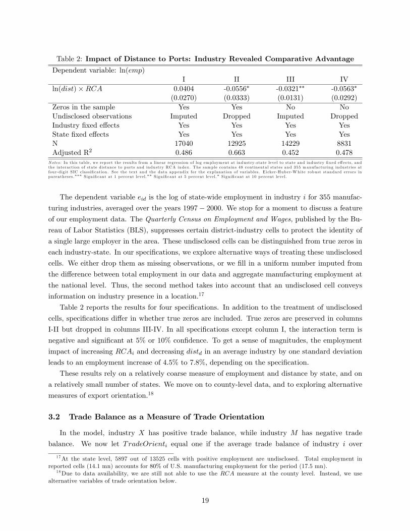
Table 2: Impact of Distance to Ports: Industry Revealed Comparative Advantage

Dependent variable: ln(emp)I II III IV

ln(dist)�RCA 0.0404 -0.0556� -0.0321�� -0.0563�

(0.0270) (0.0333) (0.0131) (0.0292)Zeros in the sample Yes Yes No NoUndisclosed observations Imputed Dropped Imputed DroppedIndustry �xed e¤ects Yes Yes Yes YesState �xed e¤ects Yes Yes Yes YesN 17040 12925 14229 8831Adjusted R2 0.486 0.663 0.452 0.478

Notes: In th is tab le, we rep ort the resu lts from a linear regression of log employm ent at industry-state level to state and industry �xed e¤ects, andthe interaction of state d istance to p orts and industry RCA index. The sample contains 48 continental states and 355 manufacturing industries atfour-d ig it SIC classi�cation . See the text and the data app endix for the exp lanation of variab les. E icker-Hub er-W hite robust standard errors inparentheses.��� Sign i�cant at 1 p ercent level.�� Sign i�cant at 5 p ercent level.� Sign i�cant at 10 p ercent level.

The dependent variable eid is the log of state-wide employment in industry i for 355 manufac-

turing industries, averaged over the years 1997� 2000. We stop for a moment to discuss a featureof our employment data. The Quarterly Census on Employment and Wages, published by the Bu-

reau of Labor Statistics (BLS), suppresses certain district-industry cells to protect the identity of

a single large employer in the area. These undisclosed cells can be distinguished from true zeros in

each industry-state. In our speci�cations, we explore alternative ways of treating these undisclosed

cells. We either drop them as missing observations, or we �ll in a uniform number imputed from

the di¤erence between total employment in our data and aggregate manufacturing employment at

the national level. Thus, the second method takes into account that an undisclosed cell conveys

information on industry presence in a location.17

Table 2 reports the results for four speci�cations. In addition to the treatment of undisclosed

cells, speci�cations di¤er in whether true zeros are included. True zeros are preserved in columns

I-II but dropped in columns III-IV. In all speci�cations except column I, the interaction term is

negative and signi�cant at 5% or 10% con�dence. To get a sense of magnitudes, the employment

impact of increasing RCAi and decreasing distd in an average industry by one standard deviation

leads to an employment increase of 4:5% to 7:8%, depending on the speci�cation.

These results rely on a relatively coarse measure of employment and distance by state, and on

a relatively small number of states. We move on to county-level data, and to exploring alternative

measures of export orientation.18

3.2 Trade Balance as a Measure of Trade Orientation

In the model, industry X has positive trade balance, while industry M has negative trade

balance. We now let TradeOrienti equal one if the average trade balance of industry i over

17At the state level, 5897 out of 13525 cells with positive employment are undisclosed. Total employment inreported cells (14.1 mn) accounts for 80% of U.S. manufacturing employment for the period (17.5 mn).

18Due to data availability, we are still not able to use the RCA measure at the county level. Instead, we usealternative variables of trade orientation below.

19

Table 3: Impact of Distance to Ports: Industry Trade Balance

Dependent variable: ln(emp)I II III IV

ln(dist)� TradeBalance -0.0216��� -0.0575��� -0.0185��� 0.00224(0.00732) (0.00892) (0.00578) (0.0145)

Zeros in the sample Yes Yes No NoUndisclosed observations Imputed Dropped Imputed DroppedIndustry �xed e¤ects Yes Yes Yes YesCounty �xed e¤ects Yes Yes Yes YesN 261545 183430 85684 22561Adjusted R2 0.456 0.425 0.291 0.413

Notes: In th is tab le, we rep ort the resu lts from a linear regression of log employm ent at industry-county level to county and industry �xede¤ects, and the interaction of county distance to p orts and a binary variab le that equals one if the industry exports exceed its imports. Thesample contains 3077 counties and 85 manufacturing industries at four-d ig it NAICS classi�cation . See the text and the data app endix for theexp lanation of variab les. E icker-Hub er-W hite robust standard errors in parentheses.��� Sign i�cant at 1 p ercent level.�� Sign i�cant at 5 p ercentlevel.� Sign i�cant at 10 p ercent level.

2001 � 2005 is positive, and zero otherwise. We also move to more disaggregated geographicalunits. Now, our dependent variable is the natural logarithm of employment at the county level

over the same time period. Employment and U.S. trade data are both available in the same

NAICS classi�cation system at the county level from the BLS and the Census Bureau Foreign

Trade Division, respectively.19

In using county-level employment data, we face tighter data disclosure limitations than with

states. Therefore, we conduct our analysis at a relatively more aggregate industry classi�cation

than with states. We consider employment in the 85 manufacturing industries at the 4-digit level of

the NAICS in 3077 counties. 27 of these industries have positive net exports and our data captures

close to 60 percent of U.S. manufacturing employment. As in the previous subsection, we estimate

(25) using two samples that treat undisclosed data di¤erently.

Table 3 reports the results. We include industry and county �xed e¤ects in all cases. We

�nd a signi�cant negative slope for the interaction term except if we drop both true zeros and

nondisclosed observations. To get a sense of magnitudes, moving toward the nearest port by one

standard deviation of the distance distribution increases employment in export oriented industries

by between 7:5% and 23% relative to import competing industries. If we consider the extremes

of the distance distribution, we have that moving inland from a representative port for 400 miles,

a value close to the 90th percentile of the distribution of distance, causes relative employment in

export-oriented industries to shrink by between 18% and 44%.

3.3 Export/Output Ratio as a Measure of Trade Orientation

In the model, the fraction of all shipments that are exported is larger in industry X than

in industry M . As an alternative measure of trade orientation we consider the exported share

19An advantage of using the trade balance for TradeOrienti, as well as the export-output ratio that we considerbelow, is that, in contrast with using RCAi, we only need U.S. data sources and we can bypass the concordancebetween trade and industry classi�cations.

20

Table 4: Impact of Distance to Ports: Industry Export Intensity

Dependent variable: ln(emp)I II III IV

ln(dist)� (EXP=Q) -0.0245 0.142��� -0.307��� -0.167���

(0.0266) (0.0325) (0.00514) (0.00437)Industries in the sample All All All AllZeros in the sample Yes Yes Yes YesUndisclosed observations Imputed Dropped Imputed DroppedIndustry �xed e¤ects Yes Yes No NoCounty �xed e¤ects Yes Yes Yes YesN 261545 183430 261545 183430R-squared 0.449 0.418 0.301 0.298

Notes: In th is tab le, we rep ort the resu lts from a linear regression of log employm ent at industry-county level to county and industry �xed e¤ects,and the interaction of county d istance to p orts and industry export/output ratio . The sample contains 3077 counties and 85 manufacturingindustries at four-d ig it NAICS classi�cation . See the text and the data app endix for the exp lanation of variab les. E icker-Hub er-W hite robuststandard errors in parentheses.��� Sign i�cant at 1 p ercent level.�� Sign i�cant at 5 p ercent level.� Sign i�cant at 10 p ercent level.

of output. Using export and industry output from the NBER-CES manufacturing dataset, we

compute the export/output ratios at the national level for the 85 industries in the sample.20 As

dependent variable we use, as before, the natural logarithm of county employment by industry.

In tables 4 and 5 we move across speci�cations that di¤er in whether we include industry �xed

e¤ects, in how we treat undisclosed observations, and in whether we break down the sample by the

industry trade balance. To avoid cluttering the presentation, we only include results with all the

zeros in the sample, and relegate results without zeros to the appendix.

Columns I and II of Table 4 report the baseline speci�cation in (25). The coe¢ cient of interest

is either not signi�cantly di¤erent from zero or has the wrong sign. In columns III-IV we repeat

the baseline speci�cation, but we do not include industry e¤ects �i. Without industry e¤ects, we

see again a signi�cant and negative gradient.

This discrepancy could arise due to several aspects of the data. One possibility is that the

export/output ratio is not a good measure of trade orientation at this level of industry aggregation.

For example, export/output ratios could vary across industries due to di¤erent levels of intra-

industry trade rather than to comparative advantages of the U.S.21 Alternatively, the distribution

of zeros and employment might be such that industry e¤ects pick up the concentration of export-

oriented industries near ports, while employment and export-output ratios vary with distance within

each type of industries due to forces not accounted for in the model.

Therefore, we repeat the speci�cations I and II of Table 4, including industry �xed e¤ects, within

subgroups of industries that di¤er in their trade balance. Table 5 reports the results for export

oriented industries in columns I-II, and for import competing industries in columns III-IV. Now,

the slopes have opposing signs for industries with di¤erent trade balance. For the export oriented

20The average export-output ratio across industries is 15%, with a standard deviation of 13%. See table 8 in theAppendix for a list of industries with their trade balance and export-output ratio.

21The correlation between export/output and import/output ratios across the 85 industries in the sample is 0.44.The mean Grubel�Lloyd index of intra-industry trade (= 1�jEXPi�IMPij=(EXPi+IMPi)), which varies between0-1 and is increasing in the extent of intra-industry trade, equals 0.69.

21

Table 5: Impact of Distance to Ports: Industry Export Intensity II

Dependent variable: ln(emp)I II III IV

ln(dist)� (EXP=Q) -0.195��� -0.530�10�5 0.0388 0.202���

(0.0557) (0.0689) (0.0300) (0.0363)Industries in the sample EXP > IMP EXP > IMP EXP < IMP EXP < IMPZeros in the sample Yes Yes Yes YesUndisclosed observations Imputed Dropped Imputed DroppedIndustry �xed e¤ects Yes Yes Yes YesCounty �xed e¤ects Yes Yes Yes YesN 83079 58266 178466 125164R-squared 0.431 0.436 0.460 0.409

Notes: In th is tab le, we run the regression describ ed in the prev ious tab le for two sub-samples of the data group ed by net exports. E icker-Hub er-W hite robust standard errors in parentheses.��� Sign i�cant at 1 p ercent level.�� Sign i�cant at 5 p ercent level.� Sign i�cant at 10 p ercentlevel.

industries � is negative, while for import competing industries it is positive. The coe¢ cient is

either statistically insigni�cant or positive, depending on how undisclosed data is treated. When

we include undisclosed cells, export oriented industries with higher export/output ratio reduce

their employment as we move further away from the nearest port (column I), while across import

competing industries there is no statistically signi�cant e¤ect (column III).

To sum up, using various measures of trade orientation and di¤erent levels of geographical

aggregation we �nd a negative correlation between industry proximity to ports and export status.

This suggests that domestic trade costs and international comparative advantages may play a role

in the location of industries. While other forces might cause this correlation, we see the result as

�rst-pass motivating evidence in support of the theory.

We move on to measuring the e¤ect of domestic trade costs on the concentration of economic

activity and the gains from trade using our model.

4 Quantitative Analysis using the Baseline Model

We propose a quantitative methodology to measure the impact of market access and compar-

ative advantages. We �rst discipline the parameters of the model matching features of the data

related to international trade. Then, we compare the model prediction for the concentration of

employment with its empirical counterpart, and we compute the counter-factual gains from trade

under alternative levels of domestic trade costs.

4.1 Calibration Strategy

For the calibration, we assume Cobb-Douglas preferences with share X in the exported good.

Since the distribution of land endowments � (`) does not a¤ect the outcome for n (`) we set it to be

uniform, � (`) = 1=`. By proper choice of units, we can normalize to one the labor to land ratio n

22

and the maximum distance to an international gate `.22 We can also set aY = 1 and write aX = a

without a¤ecting the equilibrium outcomes for the calibration or the counterfactual exercises.

Therefore we have 5 key parameters: returns to scale �, domestic trade costs �1, taste for

exported goods X , relative price at the port p(0), and relative cost in export oriented industries a.23

The �rst two parameters measure the e¤ects of domestic geography, while the last two parameters

measure the strength of comparative advantages.

The parameters X and � are chosen to match direct empirical counterparts. We set X equal

to �nal expenditures in industries where the U.S. is a net exporter as share of total expenditures

in manufacturing.24 Using 1997 US input-output tables, Herrendorf and Valeyinti (2008) impute

the cost share of land in manufacturing to be 0:03: In the model, the share of land costs in the

production of tradeables is equal to 1 � �; so we use � = 0:97 in the baseline calibration. After

fully calibrating the model, we check the robustness of results to variation around these values.

The last three key parameters fp(0); �1; ag are obtained by matching model outcomes withmoments from the data. The comparative-advantage parameter, a, is chosen to match the export

share in manufacturing output, equal to an average of 16:6% over the years 1989-2000. This is a

conventional target in the international trade literature. In turn, �1 and p (0) are chosen to match

relatively more novel targets related to the nature of our exercise.

The domestic trade cost �1 is set to match the share of domestic shipping costs in the value

of export shipments. The 1997 Commodity Flow Survey (CFS) reports the total f.o.b value for a

representative sample of export shipments. It also informs the number ton-miles for the domestic

segment of these shipments. To �nd the shipping cost associated with export-bound cargo, we use

the cost of shipping per ton-mile from U.S. Federal Highway Administration data. We compute

shipping costs to be 1:5% of the f.o.b shipment value and use this value as calibration target.25

This way of computing domestic trade costs as well as the magnitude that we �nd are similar to

Glaeser and Kollhase (2004).26

Finally, to determine p(0) we match the empirical counterpart of the domestic boundary b: In

the model, population density n(`) in (18) declines monotonically with distance between ` = 0

and b, and stays constant in�b; `�: To identify the value for b in the data, in Figure 3 we plot the

empirical counterpart of n(`) in the model. The �gure shows population density for U.S. counties

22Given our calibration strategy, choosing a di¤erent value for ` would only scale the calibrated �1 proportionallywithout a¤ecting model outcomes such as the land and population shares of the coastal region.

23We do not need to consider world prices p� or external trade costs �0 separately. What matters for modeloutcomes is the relative price at the port, p(0) = p�e��0 .

24We use U.S. manufacturing exports, imports and shipments data for six-digit NAICS. Total consumption isC = Y + IMP � EXP where Y is aggregate gross shipments, IMP is total imports and EXP is total exports.We then calculate CX as the sum of consumption in all industries that have positive trade balance. This yieldsCX=C = 0:454 for the period 1989-2000.

25The cost of a ton-mile shipment varies between 5 to 15 cents in 1997 dollars depending on the size and categoryof the truck. In the CFS data, $339 billion worth of export shipments by trucks traveled 51 billion ton-miles. At$0:1 per ton-mile, this makes shipping costs equal to 1:5% of the f.o.b shipment value. In the CFS sample morethan 60% of the value of all export bound cargo is carried to ports by trucks, so that we consider this measureme asrepresentative of domestic shipping costs.

26 In our baseline calibration of �1 = 0:38, domestic frictions are small but non-trivial: the ad-valorem equivalentvalue of shipping a good from the port is 3:9% to the boundary b and 46% to the innermost location in the territory.

23

Figure 3: Population and Density Across U.S. Counties

03

69

1215

1821

2427

3033

Den

sity

 (nor

mal

ized

)

0 .1 .2 .3 .4 .5 .6 .7 .8 .9 1

Distance (normalized)

against the measure of distance to the nearest port de�ned in Section 3, as well as its �tted spline.

Population density is normalized to the national average, and distance is expressed relative to the

most distant county. The �gure re�ects the well-known fact that population density in the U.S. is

biased toward coasts (Rappaport and Sachs, 2003).27

We see that in the data population density follows a similar pattern to the model. Population

declines fast as we move away from ports, but the slope �attens near counties separated from

their closest port by a distance equal to 10% the distance of the most distant counties.28 After

that, average density stays relatively constant as we keep moving inland. This provides a natural

mapping with the theory. Accordingly, we set b=` = 10%. Then, we use the equilibrium condition

(20), which determines the boundary, to pick p(0) such that p(b) = p(0)e�2�1b = a.29

Table 6 summarizes the parameters from our calibration. The �rst two parameters are matched

to their empirical counterparts without solving the model, while for the last three parameters we

solve the model and match the outcomes to the empirical moments.

4.2 Density in Coastal Areas

Using the calibrated model we compute the population density in the coastal region de�ned in

(21). We let bnC be the model-predicted value, and neC be the empirical value. To measure the27Since our distance measure is de�ned in relationship to the largest ports for U.S. trade, this �gure partly re�ects

population density close to some the U.S. largest airports, some of them situated in the interior of the country. Seethe de�nition of the distance measure in Section 3 and the map with the ports in the Appendix.

28The most distant location is at 570 miles, so that the change in slope happens near locations situated at about60 miles from the nearest port.

29From this expression, it is clear that only p (0) =a matters for the location of the boundary. Comparativeadvantages a then determine the trade share of GDP given the value of b.

24

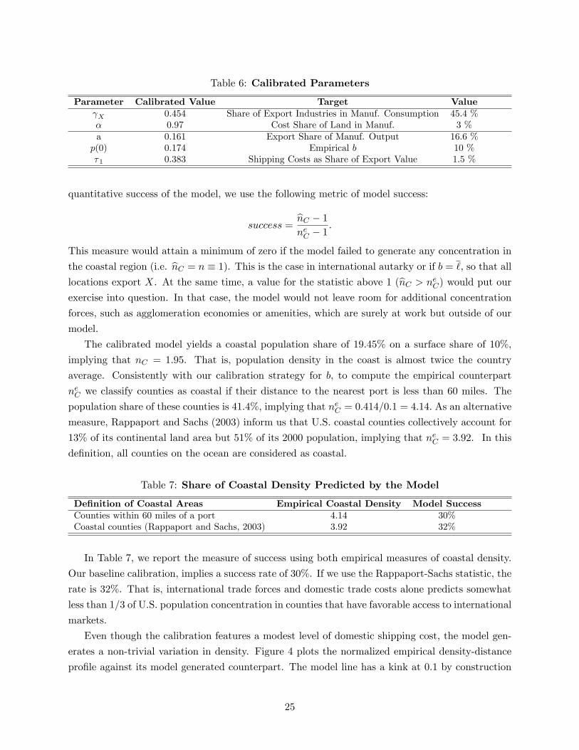
Table 6: Calibrated Parameters

Parameter Calibrated Value Target Value X 0.454 Share of Export Industries in Manuf. Consumption 45.4 %� 0.97 Cost Share of Land in Manuf. 3 %a 0.161 Export Share of Manuf. Output 16.6 %p(0) 0.174 Empirical b 10 %�1 0.383 Shipping Costs as Share of Export Value 1.5 %

quantitative success of the model, we use the following metric of model success:

success =bnC � 1neC � 1

.

This measure would attain a minimum of zero if the model failed to generate any concentration in

the coastal region (i.e. bnC = n � 1). This is the case in international autarky or if b = `, so that alllocations export X. At the same time, a value for the statistic above 1 (bnC > neC) would put ourexercise into question. In that case, the model would not leave room for additional concentration

forces, such as agglomeration economies or amenities, which are surely at work but outside of our

model.

The calibrated model yields a coastal population share of 19:45% on a surface share of 10%,

implying that nC = 1:95. That is, population density in the coast is almost twice the country

average. Consistently with our calibration strategy for b, to compute the empirical counterpart

neC we classify counties as coastal if their distance to the nearest port is less than 60 miles. The

population share of these counties is 41:4%, implying that neC = 0:414=0:1 = 4:14: As an alternative

measure, Rappaport and Sachs (2003) inform us that U.S. coastal counties collectively account for

13% of its continental land area but 51% of its 2000 population, implying that neC = 3:92. In this

de�nition, all counties on the ocean are considered as coastal.

Table 7: Share of Coastal Density Predicted by the Model

De�nition of Coastal Areas Empirical Coastal Density Model SuccessCounties within 60 miles of a port 4.14 30%Coastal counties (Rappaport and Sachs, 2003) 3.92 32%

In Table 7, we report the measure of success using both empirical measures of coastal density.

Our baseline calibration, implies a success rate of 30%. If we use the Rappaport-Sachs statistic, the

rate is 32%. That is, international trade forces and domestic trade costs alone predicts somewhat

less than 1=3 of U.S. population concentration in counties that have favorable access to international

markets.

Even though the calibration features a modest level of domestic shipping cost, the model gen-

erates a non-trivial variation in density. Figure 4 plots the normalized empirical density-distance

pro�le against its model generated counterpart. The model line has a kink at 0:1 by construction

25

Figure 4: Population Density and Distance: Model vs Data

02

46

810

12

Pop

ulat

ion 

Den

sity

 (nor

mal

ized

)

0 .1 .2 .3 .4 .5 .6 .7 .8 .9 1

Distance (normalized)

Data Model

and reaches about a third of the empirical intercept.

In the last section we perform various robustness checks and we show that the model is capable

of generating a reasonable level of concentration for an empirically relevant range of parameter

values around our calibrated values.

4.3 Domestic Trade Costs and Gains from Trade

We now use the calibrated model to study the e¤ect of domestic frictions on welfare. For

that, we vary �1 around a range of values at its calibrated value of 0:383, while keeping all other

parameters �xed. For each value of �1, we compute the coastal density, nC , and the percent gains

from trade u�=ua � 1. The results are shown in Figure 5. In each case, we highlight the calibratedvalue of �1. As we move to the right, domestic trade costs increase and the boundary b moves

towards ` = 0.

The left panel of Figure 5 shows that larger domestic trade costs lead to higher population

density in the coastal region. For a su¢ ciently low value of �1 = 0:038, b = ` and the economy fully

specializes in X. In this case population density in the coastal regions equals the country average.

The right panel presents the e¤ect on welfare. The theory tells us that domestic and interna-

tional trade costs are complementary: increasing �0 from actual values to the level that precludes

international trade has a stronger e¤ect on welfare when �1 is smaller. The gains from trade at the

calibrated value for the parameters are 0:33%, and as �1 grows they approximate zero. When �1 is

half of its calibrated value u�=ua increases to 0:63%, implying an elasticity of the gains from trade

with respect to domestic trade costs close to one near the calibrated parameters.

The elasticity increases as we reduce domestic trade costs further. In the frictionless world, with

26

Figure 5: Counterfactual Analysis of a Reduction in Domestic Trade Costs

0.0383 0.25 0.3833 0.5 0.75 11

1.25

1.5

1.75

1.9467

2.25

τ1

Coa

stal

 den

sity

  (n

c)

0.0383 0.25 0.3833 0.5 0.75 10

0.0033

0.01

0.02

0.0236

0.03

0.0427

τ1

Gai

ns f

rom

 tra

de in

 pct

. (u

* /ua ­1

)

complete specialization

completespecialization

calibrated value

calibrated value

�1 close to zero, real income is about 4:2% higher than in its autarky level. This is the upper bound

for the gains from trade, u=ua, that we de�ned in (24). Therefore, in terms of that decomposition,

we obtain:u�

ua|{z}�0:33%

= (�1; b)| {z }�1=13

� u

ua|{z}�4:2%

We conclude that domestic trade costs, despite having a small magnitude, have a potentially

large impact on the gains from trade. Since the baseline model does not include a number of

additional forces, this large e¤ect is likely an upper bound.

4.4 Robustness

We evaluate the sensitivity of the results to variation in the exogenously �xed parameters and

in the moments used to match the remaining parameters. The results do not vary considerably

with the external trade costs �0, with the preferences parameter X or with the export/output

target, but they are quite sensitive to the returns-to-scale parameter � and the domestic shipping

cost target. Figure 6 plots the model-generated coastal density in four cases, together with the

baseline value (red dashed line) and with the empirical value (black dashdot line).

First, we recalibrate the model for a range of values for � in the empirically relevant range of

[0:96; 0:98] according to estimates in the literature.30 The result is in in the upper-left panel of

30Caselli and Coleman (2001) use a value of 0:06 based on national income accounting by Jorgenson and Gollop(1992). Albouy (2012) and Rappaport (2008) report lower numbers, ranging between 0:016 and 0:025.

27

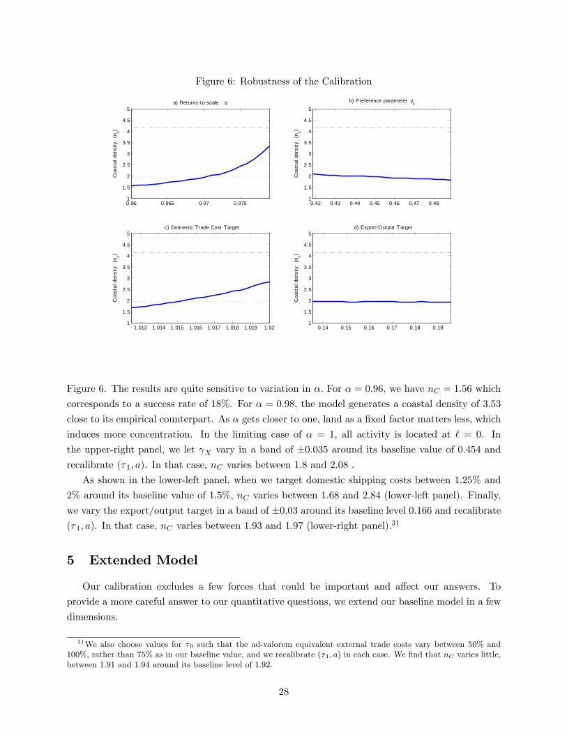
Figure 6: Robustness of the Calibration

0.96 0.965 0.97 0.9751

1.5

2

2.5

3

3.5

4

4.5

5a) Returns­to­scale α

Coa

stal

 den

sity

  (n

c)

0.42 0.43 0.44 0.45 0.46 0.47 0.481

1.5

2

2.5

3

3.5

4

4.5

5b) Preference parameter γx

Coa

stal

 den

sity

  (n

c)

1.013 1.014 1.015 1.016 1.017 1.018 1.019 1.021

1.5

2

2.5

3

3.5

4

4.5

5c) Domest ic Trade Cost Target

Coa

stal

 den

sity

  (n

c)

0.14 0.15 0.16 0.17 0.18 0.191

1.5

2

2.5

3

3.5

4

4.5

5d) Export/Output Target

Coa

stal

 den

sity

  (n

c)

Figure 6. The results are quite sensitive to variation in �: For � = 0:96, we have nC = 1:56 which

corresponds to a success rate of 18%. For � = 0:98; the model generates a coastal density of 3:53

close to its empirical counterpart. As � gets closer to one, land as a �xed factor matters less, which

induces more concentration. In the limiting case of � = 1; all activity is located at ` = 0. In

the upper-right panel, we let X vary in a band of �0:035 around its baseline value of 0:454 andrecalibrate (�1; a). In that case, nC varies between 1:8 and 2:08 .

As shown in the lower-left panel, when we target domestic shipping costs between 1:25% and

2% around its baseline value of 1:5%, nC varies between 1:68 and 2:84 (lower-left panel). Finally,

we vary the export/output target in a band of �0:03 around its baseline level 0:166 and recalibrate(�1; a). In that case, nC varies between 1:93 and 1:97 (lower-right panel).31

5 Extended Model

Our calibration excludes a few forces that could be important and a¤ect our answers. To

provide a more careful answer to our quantitative questions, we extend our baseline model in a few

dimensions.

31We also choose values for �0 such that the ad-valorem equivalent external trade costs vary between 50% and100%, rather than 75% as in our baseline value, and we recalibrate (�1; a) in each case. We �nd that nC varies little,between 1:91 and 1:94 around its baseline level of 1:92.

28

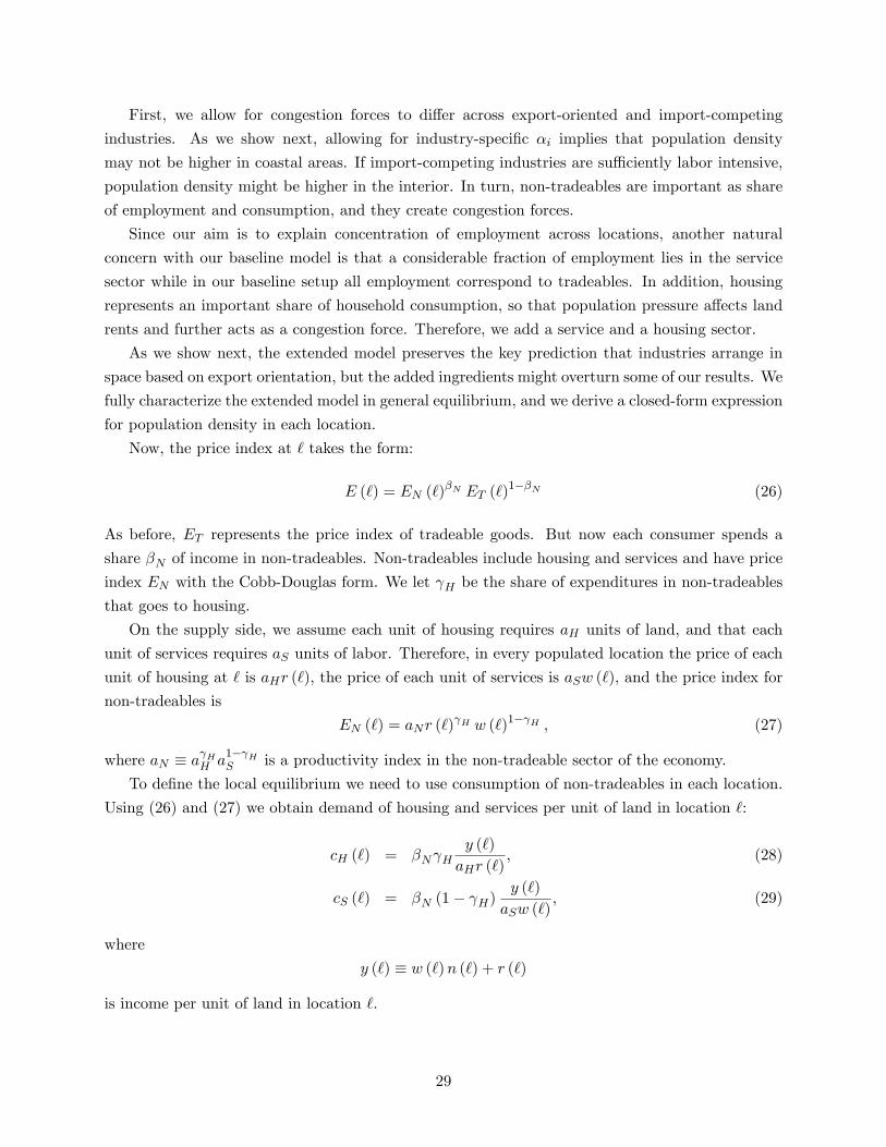
First, we allow for congestion forces to di¤er across export-oriented and import-competing

industries. As we show next, allowing for industry-speci�c �i implies that population density

may not be higher in coastal areas. If import-competing industries are su¢ ciently labor intensive,

population density might be higher in the interior. In turn, non-tradeables are important as share

of employment and consumption, and they create congestion forces.

Since our aim is to explain concentration of employment across locations, another natural

concern with our baseline model is that a considerable fraction of employment lies in the service

sector while in our baseline setup all employment correspond to tradeables. In addition, housing

represents an important share of household consumption, so that population pressure a¤ects land

rents and further acts as a congestion force. Therefore, we add a service and a housing sector.

As we show next, the extended model preserves the key prediction that industries arrange in

space based on export orientation, but the added ingredients might overturn some of our results. We

fully characterize the extended model in general equilibrium, and we derive a closed-form expression

for population density in each location.

Now, the price index at ` takes the form:

E (`) = EN (`)�N ET (`)

1��N (26)

As before, ET represents the price index of tradeable goods. But now each consumer spends a

share �N of income in non-tradeables. Non-tradeables include housing and services and have price

index EN with the Cobb-Douglas form. We let H be the share of expenditures in non-tradeables

that goes to housing.

On the supply side, we assume each unit of housing requires aH units of land, and that each

unit of services requires aS units of labor. Therefore, in every populated location the price of each

unit of housing at ` is aHr (`), the price of each unit of services is aSw (`), and the price index for

non-tradeables is

EN (`) = aNr (`) H w (`)1� H , (27)

where aN � a HH a1� HS is a productivity index in the non-tradeable sector of the economy.

To de�ne the local equilibrium we need to use consumption of non-tradeables in each location.

Using (26) and (27) we obtain demand of housing and services per unit of land in location `:

cH (`) = �N Hy (`)

aHr (`); (28)

cS (`) = �N (1� H)y (`)

aSw (`); (29)

where

y (`) � w (`)n (`) + r (`)

is income per unit of land in location `.

29

5.1 Local Equilibrium

Does the extended model preserve the key properties from the baseline setup? We can show

that, as in the baseline setup, the specialization pattern is independent from the land endowment

and depends only on each location�s distance to the port. For that, we de�ne a local equilibrium

in the extended model.

De�nition 3 (Local Equilibrium in the Extended Model) A local equilibrium at ` consists

of employment density n (`), labor demands fni (`)gi=X;M , specialization patterns f�i (`)gi=X;M ,consumption of non-tradeable goods fcS (`) ; cH (`)g, and factor prices fw (`) ; r(`)g such that

1. workers maximize utility,

w (`)

EN (`)�N ET (`)

1��N� u�; = if n (`) > 0; (30)

with demand of non-tradeables fcS (`) ; cH (`)g given by (28), (29);

2. pro�ts are maximized,

�i (`) � 0; = if �i (`) > 0, for i = X;M; (31)

where �i (`) is given by (3);

3. land and labor markets clear,

aHcH (`) +X

i=X;M

�i(`) = �(`); (32)

aScS (`) +X

i=X;M

�i(`)

�(`)ni(`) = n (`) ; and (33)

4. trade is balanced.

The de�nition of a local equilibrium is the same as in De�nition 1 except that now the land and

labor market clearing conditions (7) and (8) include resources used for housing and services. Since

�i is allowed to di¤er by sector, now conditions 2 to 4 resemble a small Hecksher-Ohlin economy

with a non-tradeable sector. As in the baseline model, specialization turns out to be independent

from land abundance. Labor mobility neutralizes factor-proportions e¤ects, and e¤ectively turns

each local economy into a Ricardian economy as in our baseline setup.

We can characterize the pattern of specialization in the local economy as follows. First, using

conditions (30) and (31), we de�ne the wage-rental ratio w (`) =r (`) that would prevail if the local

economy ` were to produce the tradeable good i:

!i (`) =

aia�N=(1��N )N

Pi (`) =ET (`)u�1=(1��N )

! 11��i+ H�N=(1��N )

if �i (`) > 0, for i = X;M . (34)

30

The wage-rental ratio decreases with the price of output Pi (`), since it increases the productivity

of land relative to other locations. A higher real wage u� naturally causes the wage-rental ratio to

increase by rising workers�outside options, as does a higher cost of living ET (`), which increases

the wage demanded by workers. A higher �i or �N increases the wage-rental rate by making the

techniques used in ` more labor intensive.

Next, we let ! (`) � w (`) =r (`) be the actual wage-rental ratio at location `. Then, (30) and(31) also imply that, in a local equilibrium,

! (`) = min f!X (`) ; !M (`)g ,

where if !X (`) < !M (`) then local economy fully specializes in X, while if !X (`) > !M (`) the

local economy fully specializes in M .

From this, we conclude that Proposition 1 also applies in the extended model. As before, the

autarky price is independent from the land endowment and therefore identical in all locations.

Hence, the pattern of specialization can be determined based on whether p (`) is above or below

pA. In contrast to the baseline model, pA is no longer equal to a but corresponds to the unique

value of p (`) for which !X (`) = !M (`). As such, it now depends on the real wage u�.

5.2 Population Density

We have just demonstrated that, as in our baseline model, the relationship between relative

prices, technology and preference parameters is su¢ cient to determine the trade pattern in each

location. As a consequence, distance to the international gate is the only fundamental characteristic

of a location that determines its specialization pattern. We conclude, as before, that whenever the

country is incompletely specialized it is partitioned into a coastal region ` 2 [0; b] and an interiorregion ` 2

�b; `�.

Before moving on to the quantitative exercise, we characterize how population density varies

based on the geographic position of each location when the country exports X to RoW. Solving for

the local equilibrium, we can show that

n (`) =

8<:�

1�N H+(1��N )(1��X)

� 1�

1!X(`)�

1�N H+(1��N )(1��A(b))

� 1�

1!X(b)

if` 2 [0; b]` 2

�b; `� . (35)

Note that for ` 2 [0; b], n (`) depends on the labor intensity in the export oriented industry, �X .In turn, for ` 2

�b; `�, intensity in land use only depends on demand conditions. In that case, we

have that �A is a weighted average of �X and �M :

�A (b) = sA (b)�X + (1� sA (b))�M

31

where the weights are given by

s (b) =a

a+ [!X (b)]�M��X � [cM=cX (p (b))]

.

and where cM=cX (p) is demand for M relative to X when the relative price of X is b implied by

the homothetic price index in the tradeable sector, ET .

As before, population in specialized regions increases towards the coast. However, the introduc-

tion of non-tradeables makes congestion forces stronger relative to a the benchmark. In addition,

when �X di¤ers from �M then n (`) is no longer continuous at the boundary b. For ` 2 [0; b], laborintensity equals �X , while for ` 2

�b; `�labor intensity depends on relative consumption in each

sector. As a consequence if �X > �M then �A < �X , and population density jumps down at the

boundary.

A general equilibrium of the extended model is then characterized by the values of fu�; bg suchthat the aggregate labor market condition (16) and condition (20) for the determination of b hold.

5.3 Quantitative Analysis with the Extended Model

[To be Completed]

6 Conclusion

We developed and quanti�ed a theory to characterize the interaction between international trade

and the geographic distribution of economic activity within countries. We presented a framework

that combines standard forces in international trade with a geographic dimension within countries.

Locations within countries di¤er in access to international markets and congestion forces deters

economic activity from concentrating in a single point.

We �nd that whenever an open economy is not fully specialized in what it exports, two dis-

tinct regions necessarily emerge: a specialized, high-population density region close to the port

that trades internationally; and a low-population density region in the interior that stays in au-

tarky. Even though space is continuous and trade costs are uniform, heterogeneous access to world

markets is su¢ cient to generate a dual economy. The model is consistent with three basic facts:

economic activity concentrates in areas with good access to international markets; international

trade integration is correlated with migration toward these areas; and comparative-advantage in-

dustries locate in these regions. I also implies that the gains from international trade are larger

when domestic trade costs are smaller.

We empirically assessed the main model prediction for industry location. Using U.S. data on

specialization at the county level, we found that U.S. export-oriented industries at the national

level are more likely to locate and to employ more workers in places situated at lower distance from

international gates such as seaports, airports or land crossings. Finally, we calibrated the model

to U.S. data to measure the importance of international trade in concentrating economic activity

32

in coastal areas, as well as the importance of domestic trade costs in hampering the gains from

trade. Our counterfactuals using the baseline model indicate that international trade can account

for approximately 1=3 of the concentration in coastal regions of the U.S., and that domestic trade

costs, despite being small, severely reduce the gains from trade.

33

References

[1] Albouy, David (2012), "What Are Cities Worth? Land Rents, Local Productivity, and the

Capitalization of Amenity Values," manuscript.

[2] Arkolakis, Costas, Arnaud Costinot, and Andrés Rodríguez-Clare (2011), "New Trade Models,

Same old Gains?", American Economic Review 102:1, pp. 94-130.

[3] Behrens, Kristian, Carl Gaigne, Gianmarco I. P. Ottaviano, and Jacques-Francoise Thisse

(2006), "Is Remoteness a Locational Disadvantage?," Journal of Economic Geography 6, pp.

347-368.

[4] Bond, Eric (1993), "Trade, factor mobility, and income distribution in a regional model with

compensating wage di¤erential," Regional Science and Urban Economics 23, pp. 67-84.

[5] Caselli, Francesco and Wilbur John Coleman II (2001), "The U.S. Structural Transformation

and Regional Convergence: A Reinterpretation," Journal of Political Economy 109:3, pp. 584-

616.

[6] Courant, Paul and Alan V. Deardor¤ (1993), "Amenities, Nontraded Goods, and the Trade of

Lumpy Countries," Journal of Urban Economics 34, pp. 299-317.

[7] Eaton, Jonathan and Samuel Kortum (2003), "Technology, Geography, and Trade," Econo-

metrica 70:5, pp. 1741-1775.

[8] Feenstra, Robert C., Robert E. Lipsey, Haiyan Deng, Alyson C. Ma, and Hengyong Mo (2004),

�World Trade Flows: 1962-2000,�NBER WP 11040.

[9] Glaeser, Edward and Janet Kollhase (2004), "Cities, Regions, and the Decline of Transport

Costs," Papers in Regional Science 83, pp. 197-228.

[10] Fujita and Mori (1996), "The role of ports in the making of major cities: Self-agglomeration

and hub-e¤ect," Journal of Development Economics 49, pp. 93-120.

[11] Hanson, Gordon (1996), "Economic integration, intraindustry trade, and frontier regions,"

European Economic Review 40, pp. 941-949.

[12] Valeyinti, Akos and Berthold Herrendorf (2008), "Measuring factor income shares at the sec-

toral level," Review of Economic Dyanmics 11, pp. 820-835.

[13] Henderson, Vernon (1982), "Systems of Cities in Closed and Open Economies," Regional Sci-

ence and Urban Economics 12, pp. 325-350.

[14] Holmes, Thomas J. and John Stevens (2004), "Spatial distribution of economic activities in

North America.", Handbok of Urban and Regional Economics, vol. 4, pp. 2797-2843.

[15] Hummels, David and Georg Schaur (2012), "Time as Trade Barrier," NBER WP 17758.

34

[16] Jorgenson, Dale W. and Frank Gollop (1992), "Productivity Growth in U.S. Agriculture: A

Postwar Perspective," American Journal of Agricultural Economics 74:3, pp. 745-750.

[17] Krugman, Paul and Raul Livas-Elizondo (1996), "Trade policy and the Third World metropo-

lis" Journal of Development Economics 49, pp. 137-150.

[18] McCaig, Brian and Nina Pavnick (2012), "Export markets and labor allocation in a poor

country," manuscript.

[19] Rauch, James (1991), "Comparative Advantage, Geographic Advantage and the Volume of

Trade," The Economic Journal 101, pp. 1230-1244.

[20] Ramondo, Natalia, Andres Rodriguez-Clare and Milagro Saborio-Rodriguez (2011), "Increas-

ing Returns and Economic Prosperity: How can Size not Matter?," manuscript.

[21] Rappaport, Jordan (2008), "Consumption amenities and city population density," Regional

Science and Urban Economics 38, pp. 533-552.

[22] Rappaport, Jordan and Je¤rey D. Sachs (2003),"The United States as a Coastal Nation,"

Journal of Economic Growth 8, pp. 5-46.

[23] Redding, Stephen (2012), "Goods Trade, Factor Mobility and Welfare," NBER WP 18008.

[24] Rossi-Hansberg, Esteban (2004), "A Spatial Theory of Trade," American Economic Review

95.

[25] Starrett, David (1978), "Market Allocations of Location Choice in a Model with Free Mobility,"

Journal of Economic Theory 17, pp. 21-37.

[26] U.S. Census Bureau (2006), �Exports from Manufacturing Establishments�.

[27] Venables, Anthony and Nuno Limao (2002), "Geographical disadvantage: a Heckscher�Ohlin�

von Thunen model of international specialization," Journal of International Economics 58.

[28] World Bank (2009), World Development Report: Reshaping Economic Geography.

35

A Proofs

Proof of Proposition 1 (i) Pro�t maximization implies that �i (`) = (Pi(`)=ai)1=(1��i)w (`)��i=(1��i).

Therefore, (6) implies that �X (`) � �M (`) ! p (`) � a and �X (`) � �M (`) ! p (`) � a.

Since autarkic locations must consume, �i (`) > 0 for i = X;M and therefore (6) implies that

�X (`) = �M (`) ! p (`) = pA = a. (ii) and (iii) follow from (12).

Proof of Lemma 1 Suppose that there is bilateral trade between locations `X ; `M at distance

� > 0. If `X is the X-exporting location in the pair, the Proposition 1 implies that p (`M ) � pA �p (`X), so that the relative price of X is larger higher in the X-exporting location. At the same

time, domestic trade costs imply that the relative price of X is strictly larger in the X-importing

location, as implied by (13), a contradiction.

Proof of Proposition 2 (i) From Lemma 1, in international autarky there is no trade between

locations within the country. Therefore, �i (`) > 0 for i = X;M and p (`) = pA for all `. This

implies that n (`) = n and, normalizing the price ofM in autarkic locations to 1, w (`) = u� �e (a)EAin all locations. (ii) With trade, if the country is net exporter of X then n (`) is given by 18. Since

p0 (`) < 0 and p=e (p) is decreasing with p, n0 (`) < 0. If the economy is net exporter of M , then

p0 (`) > 0 but n (`) = (�=1� �) (aM � u�e(p(`)))�1=(1��) so that n0 (`) < 0. (iii) If the country

is net exporter of X, all locations that trade with RoW must produce X. (15) implies that

e�2(�0+�1`)p� � p(`). Therefore, all locations ` such that e�2(�0+�1`)p� > pA specialize in X. Sincethe country is not fully specialized, there must be autarkic locations. If e�2(�0+�1`)p� < pA then

specialization X is not feasible, and the location must stay in autarky. Therefore, there must exist

b < ` such e�2(�0+�1b)p� = pA. Higher population density in the coastal region nC=nA > 1 follows

from the fact that n (`) is continuous and strictly decreasing in ` as long as �1 > 0.

Proof of Proposition 3 (i) and (ii) If pA=p� < e�2�0 but the country is in international autarky

or exports M then the no-arbitrage conditions (14) and (15) are violated. In that case, equilibrium

condition (20) implies that b < ` ! pA=p� < e2(�0+�1`). Similar reasoning applies when the

country exportsM . If e�2�0 < pA=p� < e2�0 but the country exports X orM then the no-arbitrage

conditions (14) and (15) are violated.

Proof of Proposition 4 Average population density in the interior region is:

nA =�

1� �

�a=e(a)

aX � u�

�1=(1��):

From (19), we have that @u�=@�1 < 0, @u�=@�0 < 0, @u�=@p� > 0. These shocks causes nA to

increase. At the same time, condition (20) implies that @b@�1

< 0, @b@�0

< 0, @b@p� > 0. Finally, using

(21) and the labor market clearing condition (16), the ratio of population density between the

36

coastal and interior regions can be expressed as:

nCnA

=n

nA�R `b � (`) d`R b0 � (`) d`

.

Since nA decreases and b increases with a reduction in �0 or �1 or an increase in p�, nC=nA increases

with these shocks. Since population density decreases in coastal locations�b; `�, it means that this

region experiences a decrease in population and the coastal region experiences a population increase.

Proof of Proposition 5 From the labor market clearing condition (16) and the condition (20)

for the boundary, any change in prices that is not caused by changes in�`; � (`) ; n

implies:

Z `

0

dn (`)

n(`)s (`) d` = 0. (36)

When the economy is net exporter of X, we have from (18) that

dn(`)

n(`)=

1

1� �

�dp(`)

p(`)� de (p(`))e (p(`))

� du�

u�

�(37)

Using the de�nition of "(p) and (37) in (36) we have:

du�

u�=

Z b

0[1� "(p(`))] s (`) dp(`)

p(`)d`.

For (i), we have that an increase in the terms of trade imply dp(`)=p (`) = p� for all ` 2 [0; b]. Then,(23) gives: cu�bp =

Z b

0[1� "(p (`))]s (`) d` <

Z b

0s (`) d`:

whereR b0 s (`) d` is the share of employment in export-oriented locations. For (ii), we have that

d� i1 > 0 implies dp(`)=p (`) = �`d� i1 < 0 for all ` 2 [0; b] so d(u�=ua)=d�1 < 0.

37

B Data Appendix

B.1 Construction of the distance measure

[ To be Completed ]

Figure 7: Top U.S. Ports by Export Share

B.2 Concordance between trade and industry data

[ To be Completed ]

38

Table 8: List of NAICS Manufacturing Industries Used in Section 3NAICS code Industry Trade Balance EXP/Q

3364 AEROSPACE PRODUCTS AND PARTS 1 0.4323336 ENGINES, TURBINES, AND POWER TRANSM ISSION EQUIPMENT 1 0.3543331 AGRICULTURE AND CONSTRUCTION MACHINERY 1 0.3513339 OTHER GENERAL PURPOSE MACHINERY 1 0.3383345 NAVIGATIONAL, MEASURING , ELECTROMEDICAL ETC . INSTRUMENTS 1 0.2773359 ELECTRICAL EQUIPMENT AND COMPONENTS, NESOI 1 0.2403251 BASIC CHEMICALS 1 0.2373252 RESIN , SYNTHETIC RUBBER, & ARTIFIC IAL & SYNTHETIC FIBERS 1 0.2343253 PESTIC IDES, FERTILIZERS AND OTHER AGRICULTURAL CHEMICALS 1 0.2163391 MEDICAL EQUIPMENT AND SUPPLIES 1 0.1843334 VENTILATION, HEATING , AIR -CONDITIONING ETC. EQUIPMENT 1 0.1703259 OTHER CHEMICAL PRODUCTS AND PREPARATIONS 1 0.1513112 GRAIN AND OILSEED MILLING PRODUCTS 1 0.1243256 SOAPS, CLEANING COMPOUNDS, AND TOILET PREPARATIONS 1 0.0953122 TOBACCO PRODUCTS 1 0.0923366 SHIPS AND BOATS 1 0.0833324 BOILERS, TANKS, AND SHIPPING CONTAINERS 1 0.0813261 PLASTICS PRODUCTS 1 0.0803116 MEAT PRODUCTS AND MEAT PACKAGING PRODUCTS 1 0.0793255 PAINTS, COATINGS, AND ADHESIVES 1 0.0773222 CONVERTED PAPER PRODUCTS 1 0.0633119 FOODS, NESOI 1 0.0623362 MOTOR VEHICLE BODIES AND TRAILERS 1 0.0573111 ANIMAL FOODS 1 0.0543231 PRINTED MATTER AND RELATED PRODUCT, NESOI 1 0.0493133 FIN ISHED AND COATED TEXTILE FABRICS 1 0.0463321 CROWNS, CLOSURES, SEALS AND OTHER PACKING ACCESSORIES 1 0.0113343 AUDIO AND VIDEO EQUIPMENT 0 0.6263344 SEM ICONDUCTORS AND OTHER ELECTRONIC COMPONENTS 0 0.4533341 COMPUTER EQUIPMENT 0 0.4513161 LEATHER AND HIDE TANNING 0 0.4063314 NONFERROUS METAL (EXCEPT ALUMINUM) AND PROCESSING 0 0.3863159 APPAREL ACCESSORIES 0 0.3543333 COMMERCIAL AND SERVICE INDUSTRY MACHINERY 0 0.3023169 OTHER LEATHER PRODUCTS 0 0.2913332 INDUSTRIAL MACHINERY 0 0.2803346 MAGNETIC AND OPTICAL MEDIA 0 0.2523399 M ISCELLANEOUS MANUFACTURED COMMODITIES 0 0.2293353 ELECTRICAL EQUIPMENT 0 0.2273329 OTHER FABRICATED METAL PRODUCTS 0 0.2253363 MOTOR VEHICLE PARTS 0 0.2133335 METALWORKING MACHINERY 0 0.1923342 COMMUNICATIONS EQUIPMENT 0 0.1913132 FABRICS 0 0.1863272 GLASS AND GLASS PRODUCTS 0 0.1753325 HARDWARE 0 0.1723369 TRANSPORTATION EQUIPMENT, NESOI 0 0.1703352 HOUSEHOLD APPLIANCES AND MISCELLANEOUS MACHINES, NESOI 0 0.1573162 FOOTWEAR 0 0.1463262 RUBBER PRODUCTS 0 0.1413322 CUTLERY AND HANDTOOLS 0 0.1373271 CLAY AND REFRACTORY PRODUCTS 0 0.1363365 RAILROAD ROLLING STOCK 0 0.1363313 ALUM INA AND ALUMINUM AND PROCESSING 0 0.1333254 PHARMACEUTICALS AND MEDICINES 0 0.1293221 PULP, PAPER, AND PAPERBOARD MILL PRODUCTS 0 0.1273152 APPAREL 0 0.1263351 ELECTRIC LIGHTING EQUIPMENT 0 0.1243361 MOTOR VEHICLES 0 0.1043279 OTHER NONMETALLIC M INERAL PRODUCTS 0 0.0983211 SAWMILL AND WOOD PRODUCTS 0 0.0953311 IRON AND STEEL AND FERROALLOY 0 0.0953326 SPRINGS AND W IRE PRODUCTS 0 0.0933149 OTHER TEXTILE PRODUCTS 0 0.0853141 TEXTILE FURNISHINGS 0 0.0613212 VENEER, PLYWOOD, AND ENGINEERED WOOD PRODUCTS 0 0.0603114 FRUIT AND VEGETABLE PRESERVES AND SPECIALTY FOODS 0 0.0573131 FIBERS, YARNS, AND THREADS 0 0.0523151 KNIT APPAREL 0 0.0503372 OFFICE FURNITURE (INCLUDING FIXTURES) 0 0.0493117 SEAFOOD PRODUCTS PREPARED, CANNED AND PACKAGED 0 0.0443113 SUGAR AND CONFECTIONERY PRODUCTS 0 0.0413241 PETROLEUM AND COAL PRODUCTS 0 0.0393371 HOUSEHOLD AND INSTITUTIONAL FURNITURE AND KITCHEN CABINETS 0 0.0363327 BOLTS, NUTS, SCREWS ETC. PRODUCTS 0 0.0353121 BEVERAGES 0 0.0273219 OTHER WOOD PRODUCTS 0 0.0213312 STEEL PRODUCTS FROM PURCHASED STEEL 0 0.0193115 DAIRY PRODUCTS 0 0.0183315 FOUNDRIES 0 0.0163323 ARCHITECTURAL AND STRUCTURAL METALS 0 0.0163118 BAKERY AND TORTILLA PRODUCTS 0 0.0133274 LIME AND GYPSUM PRODUCTS 0 0.0133379 FURNITURE RELATED PRODUCTS, NESOI 0 0.0123273 CEMENT AND CONCRETE PRODUCTS 0 0.004

Notes: Trade balance equals one if exp orts exceed imports over 1997-2000, and zero otherw ise. (EXP=Q) is exp ort/output ratio .

39