WP/06/104

Market-Based Estimation of Default Probabilities and Its Application to

Financial Market Surveillance

Jorge A. Chan-Lau

© 2006 International Monetary Fund WP/06/104

IMF Working Paper

Monetary and Financial Systems Department

Market-Based Estimation of Default Probabilities and Its Application to Financial Market Surveillance

Prepared by Jorge A. Chan-Lau1

Authorized for distribution by David D. Marston

April 2006

Abstract

This Working Paper should not be reported as representing the views of the IMF. The views expressed in this Working Paper are those of the author(s) and do not necessarily represent those of the IMF or IMF policy. Working Papers describe research in progress by the author(s) and are published to elicit comments and to further debate.

This paper reviews a number of different techniques for estimating default probabilities from the prices of publicly traded securities. These techniques are useful for assessing credit exposure, systemic risk, and stress testing financial systems. The choice of techniques was guided by their ease of implementation and their applicability to a wide cross-section of countries and markets. Simple one-period cases are studied to sharpen the reader’s intuition, and the usefulness of each technique for enhancing financial surveillance is illustrated with real applications. JEL Classification Numbers: G12, G15, G2 Keywords: Default probability, security prices, systemic risk, financial surveillance. Author(s) E-Mail Address: jchanlau@imf.org

1 The paper benefited greatly from discussions on credit risk modeling and derivatives pricing with Arnaud Jobert, Janet Kong, Yinqiu Lu, André Santos, and especially Amadou Sy. All errors and omissions are my sole responsibility.

- 2 -

Contents Page

I. Market-Based Default Probabilities and Financial Surveillance............................................3

II. Credit Default Swaps ............................................................................................................4

III. Bonds ...................................................................................................................................7

IV. Equity Prices........................................................................................................................9

V. From Risk-Neutral Probabilities to Real-World Probabilities............................................13

VI. Conclusions........................................................................................................................14

References................................................................................................................................16 Figures 1. Argentina: Maximum Recovery Rate and 5-Year Default Probability .................................6 2. Brazil, Sovereign Default Probability, 2001–05....................................................................8 3. Dah-Sing Bank: Distance-to-Default...................................................................................10 4. General Motors: 5-Year Default Probability .......................................................................12 5. Korea, Malaysia, and Thailand: Expected Number of Defaults ..........................................12 6. General Motors: 5-Year Risk-Neutral and Real-World Default Probabilities.....................14

- 3 -

I. MARKET-BASED DEFAULT PROBABILITIES AND FINANCIAL SURVEILLANCE

Estimating default probabilities for individual obligors is the first step when assessing the credit exposure and potential losses faced by an investor or financial institutions. From a policy perspective and for regulatory purposes, it is also the first step in evaluating systemic risk and stress testing financial systems at the national, regional, and global level. In particular, once the default probabilities of a subset of obligors are known, it is straightforward to estimate the associated loss distribution, a key ingredient for assessing risks and vulnerabilities in the corporate and financial system.2 Estimating default probabilities, however, could be challenging owing to limitations on data availability. Fortunately, there are a number of techniques that allow us to overcome these limitations. These techniques can be broadly classified into two categories: market-based techniques, which rely on security prices and ratings, and fundamental-based techniques, which rely on financial statement data and/or systematic market and economic factors. The purpose of this paper is to review a number of different techniques for estimating default probabilities using market-based information and to illustrate their usefulness for financial surveillance. Whenever possible, the analysis of simple, one-period cases is included to sharpen the reader’s intuition. Each technique is illustrated with an example using real data obtained from Bloomberg LLP. The choice of techniques was guided by their ease of implementation. Indeed, some of the examples presented here were solved using basic Excel tools. Unfortunately, this guidance left out more powerful but also more technically demanding techniques. Learning the ropes using simpler models, however, may encourage the reader to explore this area further. Also, one advantage of simpler methods is that data requirements are lower, and hence, they are applicable for a wider cross-section of countries and markets. Market-based techniques can be applied whenever there is a relatively liquid secondary market for securities issued by, or credit derivatives referencing, the obligor or entity of interest. Under the assumption of market efficiency, securities and credit derivatives prices are forward-looking and capture all publicly available information on the default risk of an obligor. Because market prices are observable, market-based techniques rely on reverse-engineering asset pricing formulas for extracting the obligor’s default probability. The paper explains the reverse-engineering process for different types of securities. Namely, Section II explains how to obtain the default probabilities implied from credit default swaps. These instruments, which are deemed the cleaner measure of credit risk, may not be available in many countries and markets. In their absence, it is possible to use prices and spreads of corporate and sovereign bonds, a topic explored in detail in Section III. Even when fixed income markets are underdeveloped, most countries have domestic stock markets. Therefore, Section IV explains how equity price and balance sheet information can go a long way in disclosing the default risk of a firm. 2 See, for instance Chan-Lau and Gravelle (2005).

- 4 -

We should note, though, that the default probabilities so obtained are referred to as “risk-neutral” or “risk-adjusted” probabilities since they are corrected to reflect investors’ risk aversion. Risk-neutral probabilities, therefore, can be very different from real world probabilities. Therefore, Section V introduces a simple method to recover real world probabilities from their risk-neutral counterparts. Section VI concludes.

II. CREDIT DEFAULT SWAPS

Credit default swaps (CDSs) are the most liquid contracts in the credit derivatives universe. These contracts are analogous to insurance against default; the buyer of the credit derivative contract, or protection buyer, pays a quarterly fee, or CDS spread, in exchange for protection against the default of a reference obligor during the life of the contract. If the obligor defaults, the protection buyer delivers the bond or loan of the reference obligor to the protection seller in exchange for the face value of the bond or loan. CDS contracts are available for a wide universe of firms in continental Europe, Japan, United Kingdom, and the United States, emerging market sovereign issuers and some selected emerging market corporations. The typical contract maturity is 5 years for corporates, and from 1 to 10 years for sovereign issuers. CDS spreads are quoted as spreads over the swap curve rather than the Treasuries curve, as the former curve better reflects the funding costs faced by market participants. Clearly, the CDS spread price depends heavily on the default probability of the reference obligor, a fact exploited by Chan-Lau (2003, 2005) and Neftci, Santos, and Lu (2005) for predicting sovereign defaults using credit default swap spreads. This dependence is illustrated in the next one-period example. Assume a one-period CDS contract with a unit notional amount. The protection seller is exposed to an expected loss, L, equal to (1) (1 )L p RR= − , where p is the default probability, and RR is the expected recovery rate at default. The recovery rate and default are assumed to be independent. In the absence of market frictions, fair pricing arguments and risk neutrality imply that the CDS spread, S, or “default insurance” premium, should be equal to the present value of the expected loss:

(2) (1 )1

p RRSr

−=

+,

where r is the risk-free rate. The default probability can be recovered from (2) if the recovery rate, the CDS spread, and the discount factor are known. We illustrate more generally how to extract the default probability from a CDS contract with maturity T using the constant hazard model of Duffie (1999).3 Assume the CDS spread is

3 Assuming a constant hazard rate is appropriate when the CDS contracts are available for only one maturity, as is the case for most corporate CDS. When prices for CDS contracts

(continued…)

- 5 -

paid in periods T(i), i=1,..,n, where T=T(n), and that the default probability in period T(i) is given by (3) ( )( ( )) 1 T ip T i e λ−= − . Therefore, the CDS spread, S(T), is given by the following equation:

(4) ( , )( ) (1 )( , )

B TS T RRA Tλλ

= − ,

where RR is the expected recovery rate at default, and A and B are given by

1

[ ( )] ( )

1

( ) ( ) ( 1) ( )

( , ) ( ) ... ( ),

( ) ,( , ) ( ) ... ( ),

( ) ( ),

n

y i T ii

n

y i T i T i T ii

A T a a

a eB T b b

b e e e

λ

λ λ

λ λ λ

λλ λ λ

λ

− +

− − − −

= + +

=

= + +

= −

where y(i) is the risk-free yield corresponding to period T(i). Therefore, given data on the risk-free yield curve and the expected recovery rate, it is possible to extract the hazard rate from equation (4) and estimate the default probability using equation (3). This procedure is illustrated in the following example. Example 1. GMAC: 1-Year default probabilities General Motors Assurance Company (GMAC), the financing arm of General Motors, has been under pressure recently owing to the problems faced by its parent company, which was downgraded to junk status in May 2005. In March 21, 2005, the 1-year CDS spread was 365 basis points (bps), and the 6-month and 1-year swap rates were 3.308 percent and 3.585 percent, implying 6-month and 1-year forward default probabilities of 6 percent and 12 percent, respectively. By December 6, 2005, the 1-year CDS spread rose to an all-time high of 715 bps with the 6-month and 1-year swap rates standing at 4.676 percent and 4.713 percent, respectively. The corresponding 6-month and 1-year default probabilities jumped to 11 percent and 23 percent, respectively.

with different maturities are available, it is possible to recover a time-varying hazard rate function from standard CDS pricing models such as those presented in Duffie (1999), and Hull and White (2000).

- 6 -

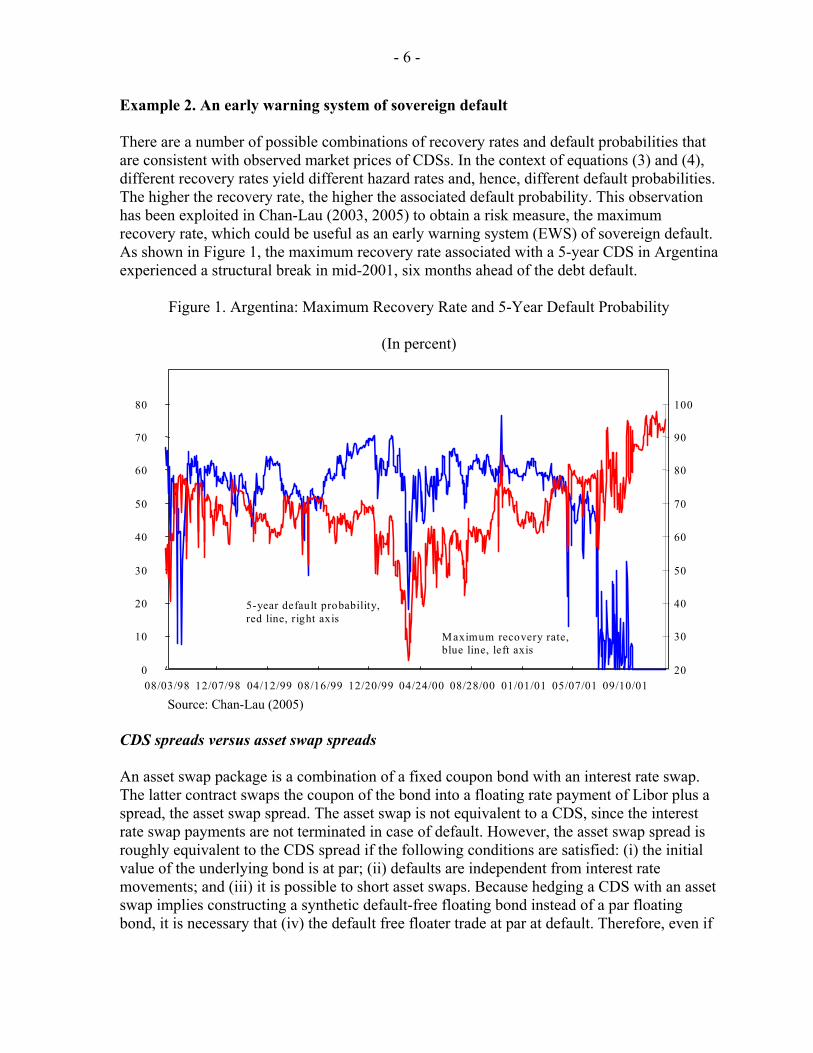
Example 2. An early warning system of sovereign default There are a number of possible combinations of recovery rates and default probabilities that are consistent with observed market prices of CDSs. In the context of equations (3) and (4), different recovery rates yield different hazard rates and, hence, different default probabilities. The higher the recovery rate, the higher the associated default probability. This observation has been exploited in Chan-Lau (2003, 2005) to obtain a risk measure, the maximum recovery rate, which could be useful as an early warning system (EWS) of sovereign default. As shown in Figure 1, the maximum recovery rate associated with a 5-year CDS in Argentina experienced a structural break in mid-2001, six months ahead of the debt default.

Figure 1. Argentina: Maximum Recovery Rate and 5-Year Default Probability

(In percent)

0 10 20 30 40 50 60 70 80

08/03/98 12/07/98 04/12/99 08/16/99 12/20/99 04/24/00 08/28/00 01/01/01 05/07/01 09/10/01 20

30

40

50

60

70

80

90

100

5-year default probability,red line, right axis

Maximum recovery rate,blue line, left axis

Source: Chan-Lau (2005) CDS spreads versus asset swap spreads An asset swap package is a combination of a fixed coupon bond with an interest rate swap. The latter contract swaps the coupon of the bond into a floating rate payment of Libor plus a spread, the asset swap spread. The asset swap is not equivalent to a CDS, since the interest rate swap payments are not terminated in case of default. However, the asset swap spread is roughly equivalent to the CDS spread if the following conditions are satisfied: (i) the initial value of the underlying bond is at par; (ii) defaults are independent from interest rate movements; and (iii) it is possible to short asset swaps. Because hedging a CDS with an asset swap implies constructing a synthetic default-free floating bond instead of a par floating bond, it is necessary that (iv) the default free floater trade at par at default. Therefore, even if

- 7 -

there are no CDSs on an obligor, if there is a liquid asset swap market it is possible to apply the techniques described in this section to extracting default probabilities.

III. BONDS

Bond prices also provide information about default probabilities as illustrated in the next one-period example. Assume a zero-coupon bond paying one unit of value at maturity. The default probability of the bond is p, the fixed recovery rate is RR, and the risk-free discount rate is r. If the bond is currently valued at B, risk neutrality implies:

(5) (1 )1p pRRB

r− +

=+

.

Equation (5) can be solved for the probability of default as a function of the recovery rate, the risk-free discount rate, and the price of the bond:

(6) 1 (1 )1

r BpRR

− +=

−.

The intuition derived from the previous example has been generalized by Fons (1987) under the assumption of risk neutrality. For a bond with N periods to redemption and a notional principal of 100, its price in period t, B(t), is given by its expected discounted cash flow:

(7) 1 2

1 2

( ) ( ) (100 )...1 1 1

t t t Nt

t t Nt

E C E C E CBr r r

+= + + +

+ + +,

where rit is the risk-free rate corresponding to each cash flow period. Assume a flat term structure of default probabilities, or equivalently, that the probability of defaulting in any of the coupon periods is the same, i.e., pt1 = pt2 = .. .= ptN = pt,. If the recovery rate, RR, and the coupon payments, C, are constant, equation (5) can be rewritten as

(8)

2

1 2

1

[(1 ) ] [(1 ) (1 )]1 1

[(1 ) (1 ) ]( 100)...1

t t t t tt

t t

N Nt t t

Nt

p RRp p RRp p CBr r

p RRp p Cr

−

− + − + −= +

+ +

− + − ++ +

+

Equation (8) can be used to back up the default probability pt if the current bond price, the recovery rate, the coupon, and the risk-free yield curve are known. In addition, the probability of experiencing a default in the next M coupon payments is given by (9) 1 (1 )M

M tP p= − − .

- 8 -

Example 3. Brazil, sovereign default probability, 2001–05 The method described above was used to evaluate Brazil’s sovereign risk during the period January 2001 to December 2005, as illustrated in Figure 3.4 Sovereign risk rose dramatically in the second half of 2002, as market confidence eroded rapidly due to uncertainty surrounding that year’s presidential election. Once it became clear that the economic policies pursued by the newly elected administration were not going to differ significantly from those of the departing administration, sovereign risk subsided rapidly.

Figure 2. Brazil, Sovereign Default Probability, 2001–05

(In percent)

5

10

15

20

25

30

01/08/01 07/02/01 12/20/01 06/18/02 12/04/02 05/30/03 11/17/03 05/11/04 10/28/04 04/21/05 10/11/055

10

15

20

25

30

Source: Bloomberg LLP, and author’s calculations. Bond spreads versus CDS spreads Bond prices are quoted as spreads over treasury bond yields, which raises the question of whether bond spreads could be used for estimating default probabilities. The answer is yes, provided that the right spread is used. No arbitrage arguments show that the CDS spread should be equal to the spread over LIBOR, or Z-spread, of a bond trading at par, or par spread (Duffie, 1999, and Hull and White, 2000). The Z-spread of the bond, however, is not exactly equal to the CDS spread and should be adjusted to account for the fact that the bond may not be trading at par, different coupon convention payments, the treatment of coupons in

4 The bond used in the analysis is the U.S.-dollar-denominated 8 percent coupon Brazilian C-bond with expiration date April 15, 2014. The assumed recovery rate is 25 percent, in line with standard market practice. Cash flows were discounted using the U.S. dollar swap curve, which is available for the following maturities: one week, 3 and 6 months, and 1, 2, 3, 4, 5, 6, 7, 8, 9, 10, 15, 20, and 30 years. Cubic splines were used to interpolate between maturities.

- 9 -

the event of default, and the potential cost to unwind a bond position. The adjusted Z-spread, then, can be used to estimate default probabilities using the procedure described in Section II. It should be kept in mind, though, that technical factors affecting market liquidity may cause even adjusted Z-spreads to be different from CDS spreads (Chan-Lau, 2003). If both CDS spreads and bond spreads are available, there remains the question of price discovery, or what instrument captures first changes in default risk. Empirical evidence suggests that price discovery takes place first in the CDS market referencing corporate issuers in advanced economies, as liquidity in the former market exceeds that of the cash bond market (Blanco, Brennan, and Marsh 2005). In the case of emerging market sovereign issuers, no particular market dominates the price discovery process (Chan-Lau and Kim, 2005).

IV. EQUITY PRICES

Black and Scholes (1973) and Merton (1974) first drew attention to the insight that corporate securities are contingent claims on the asset value of the issuing firm.5 This insight is clearly illustrated in the simple case of a firm issuing one unit of equity and one unit of a zero-coupon bond with face value D and maturity T. At expiration, the value of debt, BT, and equity, ET, are given by: (10) min( , ) max( ,0)T T TB V D D D V= = − − , (11) max( ,0)T TE V D= − , where VT is the asset value of the firm at expiration. The interpretation of equations (10) and (11) is straightforward. Bondholders only get paid fully if the firm’s assets exceed the face value of debt; otherwise, the firm is liquidated and assets are used to compensate them partially. Equity holders, thus, are residual claimants in the firm since they only get paid after bondholders. Note that equations (10) and (11) correspond to the payoff of standard European options. The first equation states that the bond value is equivalent to a long position on a risk-free bond and a short position on a put option with strike price equal to the face value of debt. The

5 Models built on the insight of Black and Scholes, and Merton, are known in the literature as structural models. Jarrow (2001) has suggested that the contingent claim analogy is not needed to extract default probabilities from equity prices and instead proposed using a reduced form model, i.e., the default process follows an exogenous process. Jarrow’s methodology is implemented empirically in Janosi, Jarrow, and Yildirim (2003). This paper does not discuss Jarrow’s methodology since it relies on rather advanced mathematic techniques.

- 10 -

second equation states that equity value is equivalent to a long position on a call option with strike price equal to the face value of debt. Given the standard assumptions underlying the derivation of the Black-Scholes option pricing formulas, the default probability in period t for a horizon of T years is given by the following formula:

(12)

2

ln ( )2

t A

tA

V r TDp N

T

σ

σ

⎡ ⎤+ −⎢ ⎥

= −⎢ ⎥⎢ ⎥⎢ ⎥⎣ ⎦

,

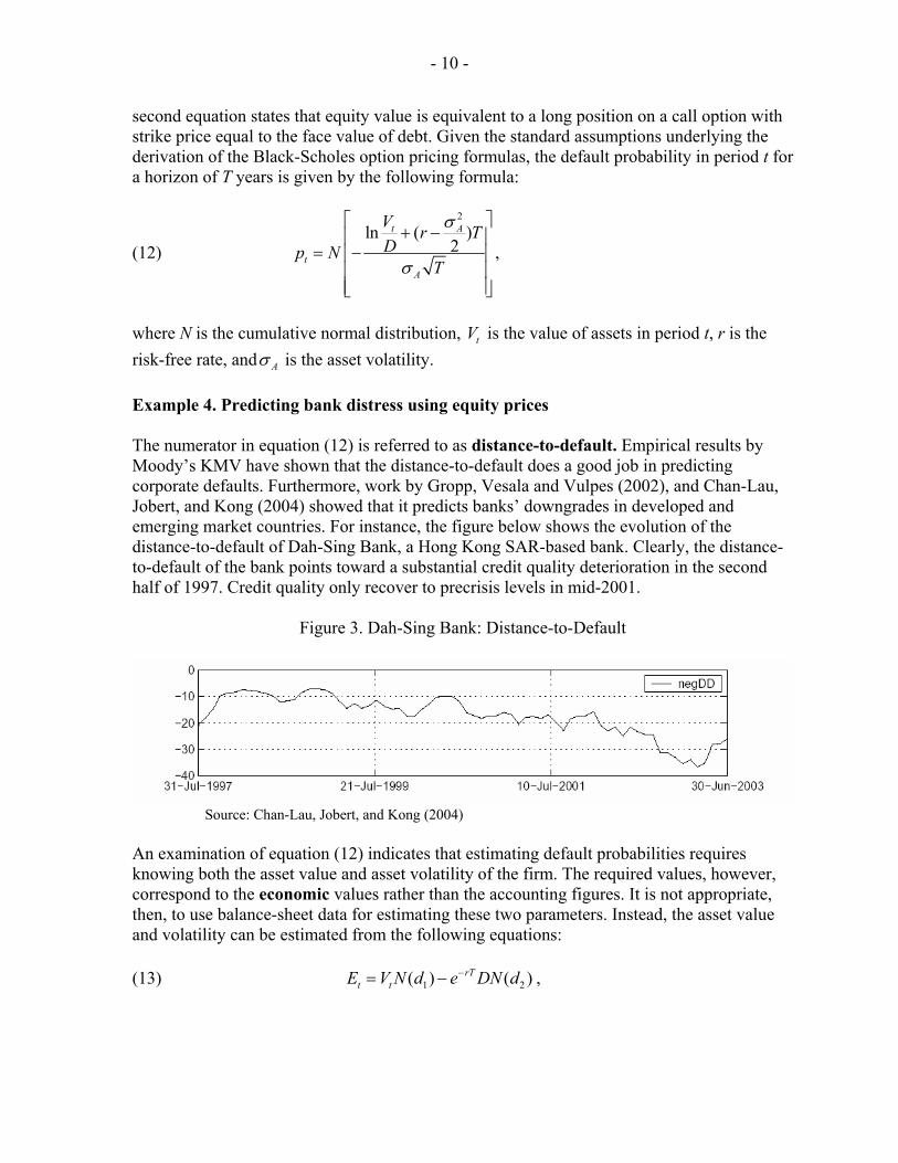
where N is the cumulative normal distribution, tV is the value of assets in period t, r is the risk-free rate, and Aσ is the asset volatility. Example 4. Predicting bank distress using equity prices The numerator in equation (12) is referred to as distance-to-default. Empirical results by Moody’s KMV have shown that the distance-to-default does a good job in predicting corporate defaults. Furthermore, work by Gropp, Vesala and Vulpes (2002), and Chan-Lau, Jobert, and Kong (2004) showed that it predicts banks’ downgrades in developed and emerging market countries. For instance, the figure below shows the evolution of the distance-to-default of Dah-Sing Bank, a Hong Kong SAR-based bank. Clearly, the distance-to-default of the bank points toward a substantial credit quality deterioration in the second half of 1997. Credit quality only recover to precrisis levels in mid-2001.

Figure 3. Dah-Sing Bank: Distance-to-Default

Source: Chan-Lau, Jobert, and Kong (2004)

An examination of equation (12) indicates that estimating default probabilities requires knowing both the asset value and asset volatility of the firm. The required values, however, correspond to the economic values rather than the accounting figures. It is not appropriate, then, to use balance-sheet data for estimating these two parameters. Instead, the asset value and volatility can be estimated from the following equations: (13) 1 2( ) ( )rT

t tE V N d e DN d−= − ,

- 11 -

(14) 1( )tE

t

V N dE

σ = ,

where Eσ is the equity price volatility, and d1 and d2 are given by:

(15)

2

1

ln ( )2

t A

A

V r TDd

T

σ

σ

+ −= ,

(16) 2 1 Ad d Tσ= − . It is possible to solve equations (13) and (14) for the asset value and volatility if the value of equity, Et, equity volatility, Eσ , and the face value of liabilities are known. The first two parameters can be calibrated from market data: the value of equity corresponds to the market value of the firm, and the equity volatility corresponds either to historical equity volatility or implied volatility from equity options. The last parameter, the face value of liabilities, D, is usually assumed equal to the face value of short-term liabilities plus half of the face value of long-term liabilities. The time horizon T is usually fixed at one year, as based on work done by Moodys KMV. Once the asset value and volatility are estimated, it is possible to recover the default probability of the firm from equation (12). Equations (12) to (15) are used to track the credit deterioration that General Motors has experienced during the past year in the next example. Example 5. General Motors: 5-Year default probability General Motors (GM), the second-largest global corporate borrower, has struggled during the past year owing to weak sales, profit warnings, mounting pension liabilities, and declining market share in the United States. As a result, the 5-year default probability started to increase rapidly in March 2005 prior to GM’s downgrade to junk status by Standard & Poor’s in May 5, 2005. However, massive stock buying by a corporate raider supported equity prices leading to a fall in equity-implied probabilities. Equity prices were also aided by hopes of a possible turnaround, and the possibility that price discounts might allow GM to post profits for the second quarter of 2005. The bankruptcy of Delphi, an auto supplier with close links to GM, together with the failure to meet profit expectations for the second quarter of 2005 reverted the downward trend and pushed the default probability to an all-time high of 75 percent in the first week of January 2006.

- 12 -

Figure 4. General Motors: 5-Year Default Probability

(In percent)

0

10

20

30

40

50

60

70

80

9/1/2004

10/1/2004

11/1/2004

12/1/2004

1/1/2005

2/1/2005

3/1/2005

4/1/2005

5/1/2005

6/1/2005

7/1/2005

8/1/2005

9/1/2005

10/1/2005

11/1/2005

12/1/2005

0

10

20

30

40

50

60

70

80

Source: Bloomberg LLP and author’s calculations.

Example 6. Measuring corporate vulnerability in East Asia The usefulness of equity-implied probabilities for conducting real-time financial surveillance work is illustrated in Chan-Lau and Gravelle (2005). They used a structural model à la Merton and loss distribution modeling techniques to construct a corporate vulnerability indicator, the expected number of defaults (END), for three Asian countries, Korea, Malaysia, and Thailand. The END indicator captures the increase in systemic corporate sector risk during the Asian crisis in these three countries. Of interest is that although the END indicator rises in each country with the onset of the Asia crisis as expected, it continues to rise well into 2000 for Malaysia and Thailand and into early 2001 for Korea.

Figure 5. Korea, Malaysia, and Thailand: Expected Number of Defaults

K o r e a

M a la y s ia

T h a ila n d

0

5

1 0

1 5

2 0

2 5

3 0

1 1 /1 8 /9 6 7 /2 8 /9 7 4 /6 /9 8 1 2 /1 4 /9 8 8 /2 3 /9 9 5 /1 /0 0 1 /8 /0 1 9 /1 7 /0 1 5 /2 7 /0 2 2 /3 /0 3 1 0 /1 3 /0 30

5

1 0

1 5

2 0

2 5

3 0E x p e c ted N u m b er o f D e fa u l ts

Source: Chan-Lau and Gravelle (2005)

- 13 -

V. FROM RISK-NEUTRAL PROBABILITIES TO REAL-WORLD PROBABILITIES

The techniques described in the previous sections allow extracting default probabilities from the prices of a variety of financial instruments. These probabilities, however, are not real-world (or objective) probabilities but risk-neutral (or risk-adjusted) probabilities that reflect investors’ aversion to certain outcomes. As an illustration, assume that there are two equally likely outcomes for a firm: survival and default. If investors have a strong aversion to default, the risk-neutral probability would be higher than the real world probability of one-half. Investors, thus, are pricing the firm’s securities as if default were more likely to occur, and hence, punishing their prices by more than warranted by the real world probability. In other words, investors are demanding a default risk premium for facing a potential default by the firm. For pricing purposes, knowledge of the risk-neutral distribution suffices for pricing assets and eliminating arbitrage opportunities. Therefore, there is not much interest or need in the financial industry to evaluate the linkages between risk-neutral and real-world probabilities. But risk-neutral probabilities tend to paint a too pessimistic view of the world.6 Why should policymakers care about real-world probabilities? From a policy perspective, it is usually preferable to err on the conservative side. But being too conservative could impose unnecessary burdens on businesses, such as excessive regulatory capital or regulatory provisioning against potential losses, especially when stress-testing individual institutions and financial systems. It is important, then, to have tools for moving back and forth between the risk-neutral world and the real world. In contrast to some other methods recently proposed in the academic literature, this paper proposes a simple tool.7 The simplicity is achieved by modeling the default event as a Bernoulli trial, that is, a random variable with only two possible outcomes, default and no default. Assume that in case of no default, the investor is paid the face value of the security, assumed equal to 100. Otherwise, the investor receives 100 times the recovery rate, RR. It is straightforward to show that, for an investor whose wealth preferences are given by the utility function u, the risk-neutral default probability, q, and the real world default probability, p, are related by 6 In contrast, estimating real world probabilities correctly is a major concern in the insurance industry. As a result, in recent years insurance companies have been major sellers of protection in credit derivatives market. Such market activity has been justified by some on the grounds that the pricing of credit derivatives is based on risk-neutral probabilities of default that largely exceed historical, or real world, default probabilities.

7 For instance, see Ait-Sahalia and Lo (2000), Bakshi, Kapadia, and Madan (2003), Bliss and Panigirtzoglou (2004), and Liu, Shackleton, Taylor, and Xu (2004).

- 14 -

(17) '(100)

1

1 '(100 )1

q uqp q u RR

q

−=− ×

−

,

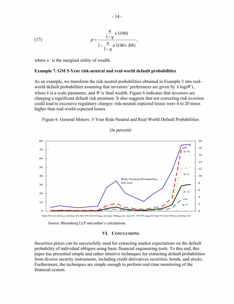
where u΄ is the marginal utility of wealth. Example 7. GM 5-Year risk-neutral and real-world default probabilities As an example, we transform the risk neutral probabilities obtained in Example 3 into real-world default probabilities assuming that investors’ preferences are given by log( )k W , where k is a scale parameter, and W is final wealth. Figure 6 indicates that investors are charging a significant default risk premium. It also suggests that not correcting risk aversion could lead to excessive regulatory charges: risk-neutral expected losses were 4 to 20 times higher than real-world expected losses.

Figure 6. General Motors: 5-Year Risk-Neutral and Real-World Default Probabilities

(In percent)

.

0

10

20 30

40 50

60

70 80

Sep-04 Oct-04 Nov-04 Dec-04 Jan-05 Feb-05Mar-05Apr-05May-05 Jun-05 Jul-05Aug-05 Sep-05 Oct-05 Nov-05 Dec-05

0

2

4

6

8

10

12

14

16

18

20

Risk-Neutral Probability,left axis

k=4

k=3

k=2

k=1

Source: Bloomberg LLP and author’s calculations.

VI. CONCLUSIONS

Securities prices can be successfully used for extracting market expectations on the default probability of individual obligors using basic financial engineering tools. To this end, this paper has presented simple and rather intuitive techniques for extracting default probabilities from diverse security instruments, including credit derivatives securities, bonds, and stocks. Furthermore, the techniques are simple enough to perform real-time monitoring of the financial system.

- 15 -

One common criticism raised against these probability estimates is that they do not reflect real-world probabilities since they may be biased upward by the presence of a default risk premium. To overcome this criticism, the paper has introduced a simple method to transform risk-neutral probabilities into real-world probabilities and vice versa. Finally, the paper has also discussed how the estimated default probabilities can be used to enhance financial market surveillance work, as they are the basic ingredients for constructing vulnerability indicators, modeling credit risk and loss distributions, and stress-testing financial systems. Indeed, work along these lines has been done or is under progress at policy institutions worldwide. But it goes without saying that much needs to be done. Hopefully, by starting to familiarize readers with the potential of financial engineering tools, this note will encourage them to think about how best to apply financial economic knowhow to policy issues.

- 16 -

REFERENCES

Ait-Sahalia, Yacine, and Andrew W. Lo, 2000, “Nonparametric Risk Management and Implied Risk Aversion,” Journal of Econometrics, Vol. 94, pp. 9–51.

Bakshi, Gurdip, Nikuni Kapadia, and Dilip Madan, 2003, “Stock Return Characteristics,

Skew Laws, and the Differential Pricing of Individual Equity Options,” Review of Financial Studies 16, pp. 101–143.

Bliss, Robert R., and Nikolaos Panigirtzoglou, 2004, “Option-Implied Risk Aversion,”

Journal of Finance 59, pp. 407–446. Black, Fischer and Myron S. Scholes, 1973, “The Pricing of Options and Corporate

Liabilities,” Journal of Political Economy 81, pp. 637–654. Blanco, Roberto, Simon Brennan, and Ian W. Marsh, 2005, “An Empirical Analysis of the

Dynamic Relationships Between Investment Grade Bonds and Credit Default Swaps,” Journal of Finance 60, pp. 2255–2281.

Chan-Lau, Jorge A., 2003, “Anticipating Credit Events using Credit Default Swaps, with an

Application to Sovereign Debt Crises,” IMF Working Paper 03/106 (Washington). Available at http://papers.ssrn.com/sol3/papers.cfm?abstract_id=414361.

———, 2005, “Credit Default Swaps, Maximum Recovery Rates, and Defaults,”

(unpublished,Washington). ———, and Toni Gravelle, 2005, “The END: A New Indicator of Financial and

Nonfinancial Corporate Sector Vulnerability,” IMF Working Paper 05/321 (Washington). Available at http://papers.ssrn.com/sol3/papers.cfm?abstract_id=876385.

Chan-Lau, Jorge A., Arnaud Jobert, and Janet Q. Kong, 2004, “An Option-Based Approach

to Bank Vulnerabilities in Emerging Markets,” IMF Working Paper 04/33 (Washington). Available at http://papers.ssrn.com/sol3/papers.cfm?abstract_id=520182.

Chan-Lau, Jorge A., and Yoon S. Kim, 2005, “Equity Prices, Credit Default Swaps, and

Bond Spreads in Emerging Markets,” The ICFAI Journal of Derivatives Markets 2, pp. 26-48. Available at http://papers.ssrn.com/sol3/papers.cfm?abstract_id=564241.

Chan-Lau, Jorge A., and Chris Morris, 2005, “Pricing Contagion: N-th to Default Credit

Default Swaps,” Global Markets Monitor, January 24. ———, and ———, 2004, “First-to-Default Swaps,” Global Markets Monitor,

November 18.

- 17 -

Duffie, Darrel J., 1999, “Credit Swap Valuation,” Financial Analysts Journal, Jan./Feb., pp. 73-87.

Fons, Jerome, 1987, “The Default Premium and Corporate Bond Experience,” Journal of

Finance 42, pp. 81-97. Gropp, Reint, Jukka Vesala, and Giuseppe Vulpes, 2002, “Equity and Bond Market Signals

as Leading Indicators of Bank Fragility,” Working Paper 150 (Frankfurt: European Central Bank).

Hull, John, and Alan White, 2000, “Valuing Credit Default Swaps I: No Counterparty

Default Risk,” Journal of Derivatives 8 (Fall), pp. 29–40. Janosi, Tibor, Robert Jarrow, and Yildiray Yildirim, 2003, “Estimating Default Probabilities

Implicit in Equity Prices,” Journal of Investment Management, First Quarter, pp. 1-30.

Jarrow, Robert, 2001, “Default Parameter Estimation Using Market Prices,” Financial

Analysts Journal 57, pp. 75-92. Liu, Xiaoquan, Mark Schackleton, Stephen Taylor, and Xinzhong Xu, 2005, “Closed-Form

Transformations from Risk-Neutral to Real-World Distributions,” unpublished. Merton, Robert C., 1974, “On the Pricing of Corporate Debt: the Risk Structure of Interest

Rates,” Journal of Finance 29, pp. 449-470. Neftci, Salih, Andre O. Santos, and Yinqiu Lu, 2005, “Credit Default Swaps and Financial

Crisis Prediction,” unpublished.