Market Liquidity as a Sentiment Indicator*

Malcolm BakerHarvard Business School

Jeremy C. SteinHarvard Economics Department and NBER

First draft: October 2001This draft: May 2002

Abstract

We build a model that helps explain why increases in liquiditysuch as lower bid-askspreads, a lower price impact of trade, or higher turnoverpredict lower subsequentreturns in both firm-level and aggregate data. The model features a class of irrationalinvestors, who underreact to the information contained in order flow, thereby boostingliquidity. In the presence of short-sales constraints, high liquidity is a symptom of the factthat the market is dominated by these irrational investors, and hence is overvalued. Thistheory can also explain how managers might successfully time the market for seasonedequity offerings, by simply following a rule of thumb that involves issuing when the SEOmarket is particularly liquid. Empirically, we find that: i) aggregate measures of equityissuance and share turnover are highly correlated; yet ii) in a multiple regression, bothhave incremental predictive power for future equal-weighted market returns.

* We thank Josh Coval, Ken French, Anthony Lynch, Andrei Shleifer, Tuomo Vuolteenaho and seminarparticipants at the Atlanta Finance Forum (Georgia Tech, Georgia State, and Emory Universities), HarvardBusiness School, and the Texas Finance Festival for helpful comments. Financial support from the Divisionof Research of the Harvard Graduate School of Business Administration (Baker) and from the NationalScience Foundation (Stein) is gratefully acknowledged.

Market Liquidity as a Sentiment Indicator

Abstract

We build a model that helps explain why increases in liquiditysuch as lower bid-askspreads, a lower price impact of trade, or higher turnoverpredict lower subsequentreturns in both firm-level and aggregate data. The model features a class of irrationalinvestors, who underreact to the information contained in order flow, thereby boostingliquidity. In the presence of short-sales constraints, high liquidity is a symptom of the factthat the market is dominated by these irrational investors, and hence is overvalued. Thistheory can also explain how managers might successfully time the market for seasonedequity offerings, by simply following a rule of thumb that involves issuing when the SEOmarket is particularly liquid. Empirically, we find that: i) aggregate measures of equityissuance and share turnover are highly correlated; yet ii) in a multiple regression, bothhave incremental predictive power for future equal-weighted market returns.

1

I. Introduction

A growing body of empirical evidence suggests that liquidity predicts stock returns, both

at the firm level and in the time series of the aggregate market. Amihud and Mendelson (1986),

Brennan and Subrahmanyam (1996), and Brennan, Chordia, and Subrahmanyam (1998) find that

measures of increased liquidity, including a low price impact of trade, low bid-ask spreads and

high share turnover, are associated with lower future returns in cross sections of individual firms.

More recently, Chordia, Roll and Subrahmanyam (2000, 2001), Hasbrouck and Seppi (2001),

and Huberman and Halka (2001) document that there is considerable time-variation in market-

wide liquidity, and Amihud (2000) and Jones (2001) show that these market-wide movements in

liquidity also forecast aggregate returns.

The traditional explanation for why liquidity might affect expected returns is a

straightforward one (Amihud and Mendelson (1986), Vayanos (1998)). Investors anticipate

having to sell their shares at some point in the future, and recognize that when they do so, they

will face transactions costs. These costs can stem either from the inventory considerations of

risk-averse market makers, or from problems of adverse selection. 1 But in either case, when the

transactions costs are greater, investors rationally discount the asset in question by more. This

story would seem to fit most naturally with the purely cross-sectional results. In particular, if we

compare two stocks, and one is observed to have permanently lower bid-ask spreads and price

impacts than the other, as well as higher turnover, it is plausible that the more liquid stock would

have a somewhat higher price, and hence lower expected returns. 1 On the former, see Demsetz (1968), Garman (1976), Stoll (1978), Amihud and Mendelson (1980), and Grossmanand Miller (1988). On the latter, see Copeland and Galai (1983), Glosten and Milgrom (1985), Kyle (1985), Easleyand O’Hara (1987) and Admati and Pfleiderer (1988).

2

It is less clear whether the same story can be carried over without modification to explain

the time-series results for the aggregate market. First of all, we do not have a well-developed

understanding of what drives the common time-series variation in measures of liquidity. For

example, though it is a possibility, it seems more of a stretch to argue that there are large swings

in the degree of asymmetric information about the market as a whole. Second, as Jones (2001)

shows, and as we verify below, the predictive power of aggregate liquidity for market returns,

particularly for equal-weighted returns, is large. In a univariate regression, a one-standard-

deviation increase in stochastically detrended turnover (equivalent to turnover going from, say,

the 1932-1998 mean of 30 percent up to 42 percent in a given year) reduces expected returns on

the CRSP equal-weighted index over the next year by approximately 13 percent.

In this paper, we develop an alternative theory to explain the connection between

liquidity and expected returns.2 More specifically, our focus is on understanding why time-

variation in liquidity, either at the firm level or for the market as a whole, might forecast changes

in returns. We implicitly accept the premise that the traditional theory is best suited to explaining

why permanent cross-firm differences in liquidity are associated with permanent cross-firm

differences in expected returns.

Our model rests on two key assumptions. First, there is a class of irrational investors, who

underreact to the information contained in order flows. The presence of these irrational investors

lowers the price impact of trades, thus boosting liquidity generally.3 Second, there are short-sales 2 Although our focus is on the stock market, the link between high prices and market liquidity seems to be pervasive.See, e.g., Shleifer and Vishny (1992) and Stein (1995) for models of the market for corporate asset sales and thehousing market, respectively. We discuss the relationship of our theory to this work below.3 Odean (1998a) and Kyle and Wang (1997) use a similar mechanism to tie overconfidence to liquidity. But thesemodels make no predictions about the relationship between liquidity and expected returns.

3

constraints. The short-sales constraints imply that irrational investors will only be active in the

market when their valuations are higher than those of rational investors—i.e., when their

sentiment is positive and when the market is, as a result, overvalued. When the sentiment of

irrational investors is negative, the short-sales constraint keeps them out of the market altogether.

Since the irrational investors tend to make the market more liquid, measures of liquidity provide

an indicator of the relative presence or absence of these investors, and hence of the level of

prices relative to fundamentals.

This theory also provides a novel perspective on a set of issues in corporate finance

which have been the focus of much work recently. Stigler (1964), Ritter (1991), Loughran and

Ritter (1995), Speiss and Affleck-Graves (1995), and Brav and Gompers (1997), among others,

find that firms that issue equity have low stock returns in the subsequent few years—this is the

so-called “new issues puzzle”. Baker and Wurgler (2000) uncover an analogous pattern in the

aggregate data: if economy-wide equity issuance is high in a given year, the market as a whole

performs poorly in the next year. The usual interpretation of these facts is that the managers

making issuance decisions are “smart money”: they have a better estimate of the long-run

fundamental value of their firms than is embodied in the current market price, and they

purposefully time their financing decisions to exploit this advantage.4

We do not dispute that this smart-money mechanism may be part of what is going on.

After all, in Graham and Harvey (2001), managers place market timing high on their list of

reasons to issue equity. However, our model offers a potentially complementary way of

4 See Stein (1996) for a model along these lines.

4

rationalizing these phenomena, without requiring a high degree of managerial timing ability.

Whether or not managers make an attempt—smart or misguided—to come up with independent

estimates of fundamental value, their financing decisions may still convey information about

future returns, if they follow a simple and plausible rule of thumb. In particular, suppose that

managers are more willing to issue equity in periods when the market for new offerings is more

liquid, in the sense of there being a reduced adverse price impact upon the announcement of a

new issue. If they behave this way, their financing choices will be a passive mirror of market

liquidity, and will thus, for the reasons outlined above, tend to forecast returns. Again, this

mechanism can work even if managers never bother to take a stand on the relationship between

prices and long-run fundamental value.

We view the contribution of this paper to be primarily a theoretical one, and as such do

not attempt to provide a definitive empirical test of the model. Nevertheless, we do briefly

examine some aggregate data on turnover, equity issuance and stock returns, and document the

following patterns. First, consistent with the corporate-finance element of our theory, there is a

very strong correlation between turnover in a given year and the share of equity in total external

finance. The simple correlation coefficient between the two variables is as high as 0.64 (in the

period prior to the deregulation of the brokerage industry), and the strength of this relationship is

largely unaffected by standard controls for valuation levels, such as the dividend-price ratio, and

past returns. Thus our premise that equity issuance is a mirror of market liquidity seems to be

borne out in the data.

5

Second, both turnover and the equity share have considerable forecasting power for year-

ahead returns, especially when we focus on an equal-weighted, as opposed to a value-weighted

index. This is true when each variable is considered separately from the other; in this respect we

are just confirming the earlier work of Jones (2001) and Baker and Wurgler (2000). Moreover, in

spite of their high correlation with one another, each plays a significant role when they are

entered in the regressions together, and the overall explanatory power for future returns is

substantially augmented. In the context of our model, this can be thought of as reflecting the

notion that both turnover and the equity share are noisy measures of “true” market liquidity.

The third message that we take away from our brief empirical exercise is that the

forecasting power of turnover appears to be large in economic terms. As already noted, in a

simple univariate regression, a one-standard-deviation increase in detrended turnover implies a

downward revision in year-ahead equal-weighted expected returns of roughly 13 percent. While

we do not have a specific calibration of the effects that might be generated by a more traditional

model, and while the standard error associated with our point estimate is large, this estimate

would appear to cast doubt on the notion that the time-variation in expected market returns arises

solely from the reaction of rational investors to fluctuations in trading costs.

The rest of the paper proceeds as follows. In Section II, we develop our basic model,

which shows how measures of secondary-market liquidity such as price impact and turnover can

forecast returns. In Section III we extend the model to incorporate firms’ equity issuance

decisions, and demonstrate how these too can forecast returns. In Section IV we discuss some of

6

the model’s implications in light of existing evidence, and in Section V we present our own

empirical results. Section VI concludes.

II. The basic model: investor sentiment and market liquidity

1. Assumptions

We model the pricing of a single stock, which is available in supply Q. There are three

dates. At time 3, the stock pays a terminal dividend of F + η + ε, where ε and η are independent

normally distributed shocks that are not made public prior to liquidation. The variance of ε is

standardized to unity. The variance of η is assumed to be infinitesimally small—in particular,

what matters is that it is small relative to the variance of ε. As will become clear, this is just an

expositional trick that simplifies the analysis slightly, by keeping the fundamental risk of the

stock—and hence the risk premium—constant from time 1 to time 2.

At time 2, there is an “insider” who obtains early private information about the value of

η, and who may trade in infinitesimally small quantities based on this private information. 5 Such

trades will partially reveal η to outside investors, and we denote by ηE the time-2 rational

expectation of η based on the information set available to outsiders. We will say more about

insider trading behavior and the inference process that determines ηE momentarily.6

5 By making the insider’s trades at time 2 small, we keep the overall supply of shares in the hands of outsiders atapproximately Q, which again simplifies the exposition by keeping the risk premium constant from time 1 to time 2.6 In our setup, the insider’s private information η is not publicly revealed until liquidation. An alternative approachis to think of η as relatively short-term private information, so that while it is made public at time 3, there is achance that the liquidating dividend is not paid out until some later time 4. It is straightforward to extend the modelin this direction. However, we need a small probability that the liquidating dividend arrives at the same time as η ismade public at time 3. Intuitively, we require that a rational investor who believes the stock to be overpriced relativeto long-run fundamentals not wish to take a long position at time 2, even if the market is underreacting to positiveinformation about η at this time. As long as there is some chance that the price will converge to fundamental valueby time 3, this condition is satisfied and our basic results go through.

7

In addition to the insider who appears at time 2, there are two types of outside investors

who are present at all times. Both types research the stock and formulate estimates of the

terminal dividend. Those investors in the first class are “smart” and have rational expectations,

so their resulting time-1 estimate of the dividend, which we denote by SV1 , is simply F. Those

investors in the second class are “dumb”, and their time-1 estimate of the dividend, DV1 , can be

either greater than or less than F. We let δ = ( )FV D −1 denote the dumb investors’ initial

“sentiment,” or misvaluation.

At time 2, when the insider trades, smart investors make a rational inference about the

implications of this trade, and incorporate it fully into their estimates of the terminal dividend.

That is, SV2 = SV1 + ηE = F + ηE. In contrast, dumb investors underreact to the information

embodied in time-2 trading activity. As a simple way of capturing this, we assume that DV2 =

DV1 + θηE = F + δ + θηE, where ½ < θ < 1. In other words, dumb investors update their

valuations in the right direction, but not far enough. 7

Both types of outside investors have constant-absolute-risk-aversion (CARA) utility. The

aggregate risk tolerance of the smart group is given by Sγ , while the aggregate risk tolerance of

the dumb group is given by Dγ . Both groups are assumed to be subject to short-sales constraints.

Thus, at time 2, one period before liquidation, the demand of the smart group, SD2 , is given by

( ){ }0,max 222 PVD SSS −= γ , (1)

7 As will become clear, the requirement that θ exceed ½ is a technical condition that ensures that our version ofKyle’s (1985) model has an interior equilibrium solution for the degree of market liquidity.

8

where P2 is the price of the stock at time 2. Similarly, the time-2 demand of the dumb group,

DD2 , is given by

( ){ }0,max 222 PVD DDD −= γ . (2)

The results that follow are driven by the interplay of two key assumptions: i) the short-

sales constraints; and ii) the fact that dumb investors underreact to the information contained in

insider trades at time 2. With respect to the former, there has been a renewed appreciation of the

potential relevance of short-sales constraints in recent work.8 In part, this reflects a growing

understanding that such constraints arise not only from the direct transactions costs associated

with shorting, but also from a variety of institutional frictions, such as the widespread tendency

for mutual-fund charters to simply prohibit the taking of short positions (Almazan et al. (2001)).

While the existence of these kinds of frictions makes it plausible that both types of outside

investors in our model might behave in a short-sales-constrained fashion, our key predictions

actually only require one of the two types to be constrained. For example, we could equally well

have the dumb group–call them retail investors–be constrained and the smart group–call them

arbitrageurs–be unconstrained.

With respect to the latter assumption, there are a number of underlying behavioral

mechanisms that might give rise to underreaction. For example, dumb investors might be

overconfident in their priors (their time-1 signal DV1 ) and hence reluctant to revise these priors

8 See, e.g., Chen, Hong and Stein (2002), D’Avolio (2002), Geczy, Musto and Reed (2002), Hong and Stein (2002),Lamont and Jones (2002) and Diether, Malloy and Scherbina (2002). Notable earlier papers include Harrison andKreps (1978), Jarrow (1980), and Diamond and Verrecchia (1987).

9

when new information comes in. Or, they may suffer from a conservatism bias (Edwards

(1968)). Or more prosaically, they may simply not be paying attention, and hence may be

unaware of the fact that anything newsworthy has happened at time 2. In any case, it is becoming

increasingly clear that a variety of stock-market phenomena can be usefully understood by

appealing to investor underreaction of this kind.9 Moreover, it is important to stress that, for our

purposes, we do not require that dumb investors underreact to all forms of information—only to

the information contained in trading activity. To the extent that this sort of news is more subtle

and less salient than say, a quarterly earnings announcement, the premise of underreaction would

seem to be all the more reasonable.10

2. Liquidity, trading volume and expected returns

Given the demand curves in (1) and (2), it is easy to solve for P2 as a function of smart

and dumb investors’ time-2 valuations, SV2 and DV2 . Moreover, once P2 has been pinned down, it

follows immediately that P1 = E1(P2). That is, P1 is just the rational expectation of P2 based on

information available at time 1, which is obtained simply by taking P2 and replacing ηE with its

ex-ante expectation of zero. This is an arbitrage relationship, because both smart and dumb

traders share the same time-1 forecast of P2, and because the one-period-ahead conditional

9 Barberis, Shleifer and Vishny (1998) and Hong and Stein (1999) argue that patterns like post-earningsannouncement drift (Bernard and Thomas (1989, 1990)) and medium-term price momentum (Jegadeesh and Titman(1993)) reflect investor underreaction to news. Hong, Lim and Stein (2000) present further evidence consistent withthe underreaction hypothesis.10 Klibanoff, Lamont and Wizman (1998) show that underreaction is greater when news is less salient.

10

variance of P2 is negligible—the only news that hits the market at time 2 is news about η, which

has infinitesimally small variance. Proposition 1 and Figure 1 summarize the results for prices.

Proposition 1: At t = {1, 2}, prices can be described by their behavior in three distinct regions

of investor sentiment.

Region 1. Low investor sentiment, SQS

tD

t VVγ

−< . In this region, only smart investors

participate in the market at time 2, and dumb investors sit out. Prices are given by SQS

tt VPγ

−= .

Region 2. Intermediate investor sentiment, DSQS

tD

tQS

t VVVγγ

+≤≤− . In this region, both

groups of investors participate in the market at time 2. Prices are given by

DSDS

D

DS

S QDt

Stt VVP

γγγγ

γ

γγ

γ

+++−⋅+⋅= .

Region 3. High investor sentiment, DQS

tD

t VVγ

+> . In this region, only dumb investors

participate in the market at time 2, and smart investors sit out. Prices are given by DQD

tt VPγ

−= .

The next step is to be more explicit about insider trading behavior at time 2, and the

associated updating process that determines ηE. To do so, we follow Kyle (1985). The insider

who observes η at time 2 is assumed to be rational and risk-neutral, and to trade by means of a

market order. Unlike the outside investors, we allow the insider to go both long and short.11 His

market order is absorbed by the pool of outside investors, who play a role analogous to that of

Kyle’s market-makers in this set-up. More precisely, since the insider’s market order is of

11 Alternatively, since the insider is risk-neutral one can equivalently think of any sales as coming from his existingholdings of the stock.

11

infinitesimal size, it only affects prices insofar as the information it contains alters outside

investors’ time-2 valuations, SV2 and DV2 .

In addition to the insider, there are also some non-strategic liquidity traders active at time

2, who place exogenously given market orders in total amount z. The variance of z is also taken

to be infinitesimally small, and for notational economy, we assume that it is the same as the

variance of η.12

While the insider observes η, he—unlike either type of outside investor—makes no

attempt to estimate F. Nor does he have any direct knowledge of δ. To keep things especially

simple, we assume that, prior to observing η, the insider’s best estimate of the terminal dividend

is simply the time-1 price P1. In other words, the insider may have a tip about an upcoming

earnings announcement, but he does not know anything else about fundamental value, and so just

relies on P1 as a summary statistic for the information about F that he does not have.13

Let the size of the insider’s market order be given by m. He seeks to maximize

E{m(F+η+ε – P2)}, which, given that his estimate of F is P1, can be written as

( ){ }2max PmE ∆−η , (3)

12 A natural extension of the model is to allow the variance of z to depend on whether or not dumb investors areparticipating in the market. To the extent that dumb investors have a greater propensity for turning over theirpositions based on local changes in their sentiment, this would lead to a higher variance of z in Regions 2 and 3. Wediscuss this extension below.13 P1 will in fact be the rational estimate of the terminal dividend for an agent who does not know F or δ if wechoose the appropriate ex ante distribution for δ. For example, suppose that δ is symmetrically distributed, andtakes on one of two values, each with probability one-half: either δ =Q/γS + Q/γD; or δ = – Q/γS – Q/γD. FromProposition 1, it follows that either P1 = F + Q/γS (Region 3); or P1 = F – Q/γS (Region 1). So P1 is an unbiasedestimator of F.

12

where ∆P2 = (P2 – P1). Intuitively, the insider trades off exploiting his private information η

against the adverse price impact of trade ∆P2. The total order flow at time 2, which we denote by

f, is given by f = m + z—i.e., the total order flow is the sum of that coming from the insider and

the liquidity traders.

Given our assumptions, ∆P2 can be written as

EwP η=∆ 2 , (4)

where w is an indicator variable that takes on the following values: w = 1 in Region 1;

DS

S

wγγ

γθθ+

−+= )1( in Region 2; and w = θ in Region 3. That is, the extent to which ∆P2

reflects a full rational-expectations reaction to the new information available at time 2 depends

on which region we are in, and hence on the sentiment parameter δ. As δ increases, and we move

from Region 1 to Region 3, the weight of the dumb traders in the pricing function increases, and

∆P2 is progressively less influenced by ηE.

The rational-expectations revision ηE, can in turn be pinned down from a regression of η

on the order flow f :

fE βη = , (5)

where ( )( )f

fvar

,cov ηβ = . So we can alternatively write ∆P2 as

ffwP λβ ≡=∆ 2 , (6)

13

where λ is the familiar Kyle (1985) depth parameter that measures the price impact of order

flow. Note that here λ = wβ , which contrasts with the standard fully rational version of the Kyle

model, where the equivalent statement is simply that λ = β .

The insider seeks to maximize his objective function as stated in Equation (3), taking the

price-impact parameter λ as given. His first-order condition is therefore:

λη2

=m. (7)

Given this expression for m, and the assumption that η and z have equal variance, we can

compute the regression parameter β as:

2412

λλ

β+

=. (8)

Recalling that λ = wβ , we have the following equilibrium condition for λ:

2412

λλ

λ+

=w

. (9)

Solving, we have that the equilibrium λ, which we denote as λ*, is given by:

412* −

=w

λ. (10)

Since w is decreasing as we move from Region 1 to Region 3, it follows from (10) that

the price impact of a trade is also decreasing. Moreover, this decreased price impact leads to

increased trading volume. To see this, note that a natural measure of expected time-2 trading

volume, which we denote by T, is simply the variance of the order flow f :

14

( ) ( ) ( ) ( )2

2

441

varvarvarvarλ

λη

+=+== zmfT

. (11)

We have thus established the following.

Proposition 2: Liquidity increases with investor sentiment. As we move from Region 1 to

Region 2 to Region 3, the market becomes more liquid at time 2, in the sense that the price

impact of a trade decreases. Correspondingly, trading volume at time 2 also increases.

The intuition for the proposition, which is illustrated in Figure 2, is very simple. As can

be seen from Equation (10), the price impact of a trade is increasing in w, which is nothing more

than a measure of the weight of the smart traders in the pricing function. In Region 1, where the

smart traders dominate the market, w is high (it equals one) and hence liquidity and trading

volume are low. At the other extreme, in Region 3, where the dumb traders dominate the market

and smart traders are sitting on the sidelines, w is low (it equals θ) and hence liquidity and

trading volume are high.

It is also worth pointing out that the results in Proposition 2 would be strengthened if we

were to follow Admati and Pfleiderer (1988) and make the variance of liquidity trading

endogenous, as opposed to keeping it a fixed exogenous constant. With optimizing liquidity

traders, any decrease in λ brought about by a decline in w will tend to feed on itself—the lower

price impact will induce liquidity traders to place more aggressive orders, thereby further

15

reducing the information content of the order flow and causing a second-round multiplier

decrease in λ.

The model’s implications for the link between liquidity and expected returns now follow

immediately. As dumb investors become more optimistic—as δ and hence DtV rise relative to

StV —not only do liquidity and trading volume increase, but expected returns fall. More

precisely, we have that:

Proposition 3: Expected returns are decreasing in liquidity. Define the expected return from

time t until the terminal date, EtR , as t

St

Et PVR −= . For t = {1, 2}, the average value of E

tR is

decreasing in dumb-investor sentiment δ and hence decreasing as we move from Region 1 to

Region 2 to Region 3. Thus, increases in market liquidity and trading volume at time 2 are

associated with a reduction in subsequent expected returns—i.e., with a reduction in ER2 .

To see the key role played by the short-sales constraint, note that if this constraint is

absent, it is as if we are always in Region 2, with both groups of investors active and the price

given by DSDS

D

DS

S QDt

Stt VVP

γγγγ

γ

γγ

γ

+++−⋅+⋅= . This is now a standard noise-trader model, as in De

Long et al. (1990). In such a case, it is still true that as dumb investors’ sentiment goes up,

expected returns fall, since dumb investors have a non-zero relative weight of DS

S

γγ

γ

+ in the

pricing formula. However, there is no longer any variation in liquidity or trading volume, since

this relative weight is now a constant for all parameter values, and w is therefore also constant at

DS

S

wγγ

γθθ+

−+= )1( . Intuitively, even if dumb investors are much more optimistic than smart

16

investors, and hence are doing all the buying, smart investors continue to exert the same

marginal influence on price, by taking short positions.

By adding the short-sales constraint to our model, we create the following new effect: as

dumb investors become more optimistic, they drive the smart investors to the sidelines and hence

gain a greater weight in the pricing function. At the extreme, in Region 3, smart investors are

completely out of the picture, and the dumb investors have a weight of unity in the pricing

function. This greater weight, combined with the assumption that dumb investors underreact to

the information contained in trades, leads to a more liquid market.

Another way to express the basic idea behind our model is to say that when the market is

observed to be highly liquid, this suggests that it is currently being dominated by dumb

investors—i.e., the inmates have taken over the asylum. And of course, in a world with short-

sales constraints, the fact that the market is being dominated by dumb investors means that the

sentiment of these dumb investors is positive, and hence that expected returns are relatively low.

Although our primary focus is on the negative correlation between liquidity and expected

returns, the model also makes another subsidiary prediction, linking liquidity to the conditional

profitability of momentum strategies. In particular, the model suggests that momentum strategies

should do better when the market is more liquid.

Proposition 4: Momentum profits are increasing in liquidity. When the market is particularly

liquid at time 2, this is because investors are underreacting to the η-information contained in the

17

order flow at this time. As a result, a strategy of buying following positive returns at time 2 and

selling following negative returns is profitable in Region 2 and Region 3, but not in Region 1.

III. A corporate-finance variation: equity issues and expected returns

It is easy to modify our model so that the notion of “liquidity” it captures is liquidity in

the market for seasoned equity offerings (SEOs). We keep the basic structure and timing as

before, and make a couple of changes. First, the insider who observes η at time 2 is no longer a

trader, but instead is the manager of the firm, who is contemplating an (infinitesimally small)

equity issue.14 We assume that the manager’s behavior can be summarized by a simple objective

function. In particular, he will issue equity if and only if

02 ≥+∆+− KPη , (12)

where K is the net present value of the investment that can be financed with the equity issue.

Thus the manager prefers to issue equity when his inside information η is unfavorable, when the

adverse price impact of an issue ∆P2 is small, and when the NPV of investment K is large.

This rendition of the manager’s objectives is similar to that of Myers and Majluf (1984),

with one crucial difference. In our formulation, the manager does not attempt to make a

comprehensive judgement of the firm’s fundamental value—i.e., he does not have an estimate of

14 Again, the reason for making the equity issue infinitesimally small is so that it does not affect the overall supplyof shares outstanding, and hence does not change the equilibrium risk premium.

18

either F or δ. Thus prior to observing η, the manager, like the insider in the previous section,

takes the price at time 1 to be a summary statistic for the expected terminal dividend.15

We use this formulation not because we believe it is necessarily the most realistic one.

Perhaps managers do in fact have some comparative advantage in judging whether their firms are

over- or undervalued relative to long-run fundamentals. But our goal is to show that even if they

are not such astute market timers, and behave in a more simple rule-of-thumb fashion that

ignores the relationship of the time-1 price to the fundamental F, their financing decisions can

still forecast subsequent returns. So long as the rule of thumb contains an element of “issue

equity when the price impact is small,” financing decisions will be a mirror of market liquidity.

And in our framework, market liquidity forecasts returns for reasons that have nothing to do with

managers being well informed about fundamentals.

The only other modification we make to the model of the previous section is to assume

that η is now uniformly, rather than normally distributed.16 As will become clear, this just

simplifies the analysis. The support of η is on [-x, x], and to avoid degenerate solutions where all

types always issue equity regardless of their draw of η, we require that K < x.

The inequality in (12) can be re-written as

0≥++− Kw Eηη , (13)

15 As noted earlier, by picking the right ex-ante distribution for δ, we can make the time-1 price the best estimate ofthe terminal dividend for an agent who does not observe either F or δ.16 Given that η has infinitesimal variance relative to ε, it is still the case that the terminal dividend is (approximately)normally distributed. So CARA utility still generates the sort of simple linear demand schedules and pricingrelationships that we have been using.

19

where w is defined as before, and where ηE is now the rational expectation of η conditional on

there being an equity issue.

Equilibrium in this version of the model consists of a threshold value of η, denoted by η*,

such that only a manager observing η ≤ η* chooses to issue equity. If managers behave this way,

then conditional on observing an equity issue, the rational inference is that:

2

* xE −=

ηη

. (14)

Plugging (14) into (13) and setting the inequality to zero, we can solve for η*:

wwxK

−−

=2

2*η. (15)

Note that η* is decreasing in w, since ( )2

*

222

wxK

dwd

−−=η , and K < x. Since η* is effectively a

measure of the intensity of equity issuance—the probability of an equity issue is given by xx

2

* +η —

it follows that equity issuance increases as we move from Region 1 to Region 3 and w falls. It is

also easy to verify that the new issues market becomes more liquid, in the sense that the

equilibrium price impact ∆P2 becomes smaller, as we move from Region 1 to Region 3. Thus we

have established:

Proposition 5: Expected returns are lower in hot issues markets. Expected returns from time 2

until the terminal date, ER2 , are lower following hot issues markets, where a “hot” market is

defined as one in which either: i) more equity issues are observed at time 2; or ii) the price

impact of an equity issue at time 2 is smaller.

20

Figure 3 provides an illustration. Again, the striking feature to be emphasized is that

financing decisions can forecast long-run returns even though managers themselves have no

view about F, the dominant component of long-run fundamental value.

IV. Discussion

We believe that the most attractive aspect of our theory is that it provides a unified

framework for thinking about two quite distinct—and at first glance, unrelated—branches of

empirical research: the body of work in market microstructure which seeks to relate measures of

liquidity and trading volume to expected returns; and the corporate-finance literature on equity

offerings and subsequent stock returns. Indeed, the theory can shed light on several more

narrowly-defined topics within these two broad areas: i) time-variation in firm-level liquidity and

stock returns; ii) the behavior of Internet stocks during that sector’s boom; iii) commonality in

liquidity across firms and its link to aggregate stock returns; iv) the firm-level new issues puzzle;

and v) economy-wide hot issue markets.

1. Firm-level liquidity and stock returns

The existing empirical evidence suggests that firm-level stock returns are increasing in

the bid-ask spread, increasing in the price impact of trade, and decreasing in trading volume.

Amihud and Mendelson (AM) (1986) sort firms into portfolios according to their bid-ask spread,

once a year from 1961 to 1980. The beta-adjusted returns of the high-spread portfolio exceed

21

those of the low-spread portfolio by 0.7 percent per month (AM Table 2). Similarly, Brennan and

Subrahmanyam (BS) (1996) sort firms into portfolios in 1984 and 1988 according an estimate of

the Kyle (1985) price-impact parameter λ. The three-year average monthly returns for the high-λ

firms (in the periods that follow) are higher than the returns on the low-λ firms by 0.6 to 1.4

percent per month (size-adjusted differences in BS Table 1). Brennan, Chordia and

Subrahmanyam (1998) find a negative relationship between lagged dollar volume and stock

returns.17 In each case, the economic significance is large, perhaps too large to square with

reasonable levels of turnover and a transaction-costs view of the liquidity premium.

It is important to note that each of these results has two components: the excess returns

come from both within-firm time-series variation in liquidity as well as between-firm variation.

Our theory can at most take partial credit for the former, while the latter is probably better

explained with the traditional transaction-costs view. We clearly have little to say about why a

firm whose stock is chronically illiquid has higher returns, year in and year out, than one whose

stock is more liquid.

Another implication of our model involves the momentum effect in stock returns. By

introducing a class of irrational investors who underreact to subtle information, we guarantee that

momentum strategies will be unconditionally profitable, fitting the results of Jegadeesh and

Titman (1993) by assumption. A somewhat more subtle prediction (Proposition 4) is that

momentum profits are conditionally more profitable when liquidity is high. Consistent with this

17 By contrast, Gervais, Kaniel and Mingelgrin (2001) find that firms that experience unusually high trading volumehave higher subsequent returns. This “high volume premium” focuses on liquidity shocks rather than the level ofliquidity and short-run rather than long-run returns, and so is not inconsistent with the basic relationship betweenhigh levels of turnover and low subsequent returns documented in Brennan, Chordia and Subrahmanyam (1998).

22

prediction, Lee and Swaminathan (2000) find that there is more momentum in stocks with high

trading volume.

2. Behavior of Internet stocks during the boom

Many of the effects in our model are vividly illustrated by the behavior of Internet stocks

during the boom period from January 1998 to February 2000. Ofek and Richardson (OR) (2001)

document that the extraordinarily high valuations in this sector at this time were accompanied by

very low bid-ask spreads and unusually high trading volume. For example, Ofek and Richardson

report a median bid-ask spread for Internet firms of 0.5 percent over this period, compared with a

statistically different 0.8 percent for non-Internet firms (OR Table 7). Similarly, turnover for

Internet firms was three times higher (OR Table 1B).

The low spreads in particular are hard to rationalize in the context of standard models of

liquidity. From an inventory-management perspective, the high volatility of Internet stocks (with

twice the variance of daily returns of non-Internet stocks) would seem to imply greater inventory

risk for market makers, and hence wider spreads. And from an adverse-selection perspective, it is

hard to imagine exogenous reasons why there should be less private information available to

market participants about the prospects of Internet firms, especially given a flow rate of news in

general (as proxied for by volatility) substantially higher than that in other industries.

In the context of our model, the explanation for the narrow spreads would begin with the

premise that the Internet sector was greatly overvalued during this period. (This would seem to

be a safe statement with 20/20 hindsight.) With short-sales constraints, this is equivalent to

23

saying that the market for Internet stocks was dominated by irrational investors. These irrational

investors were not apt to revise their valuations on the basis of subtle signals such as those

embodied in order flow. In a revealing example of just this kind of underreaction, Schultz and

Zaman (2001) and Meulbroek (2000) document that insider sales in Internet companies—unlike

similar transactions in “old economy” firms—were not accompanied by negative stock-price

impacts.18 Faced with such stickiness in valuations, it seems plausible that market makers could

safely quote narrow spreads, confident that any resulting inventory imbalances they had to

offload would be absorbed with minimal price concessions.

Our model can also explain the high turnover of Internet stocks with a corollary logic:

given the tighter spreads, it became cheaper for investors to trade, and so they did more of it.

However, this part of the story may be a bit hard to take literally, since it asserts that all of the

increase in turnover came from a reduction in the costs of trading, as opposed to an outward shift

in the demand to trade. Casual empiricism suggests that increased trading demand must also

have played an important role during the Internet boom.

It is straightforward to extend our model to capture this trading-demand effect. The key

to doing so is to assume that dumb investors are more prone to churning their positions—absent

any real information about fundamentals—than are smart investors. To be more specific, keep

aggregate dumb-investor demand exactly as before at both time 1 and time 2, but introduce some

small divergences in the relative valuations of dumb investors at time 2 only. In other words,

18 Of course, there are several possible interpretations of this finding. The first is that there was little asymmetricinformation at this time in this industry. The second is that Internet insiders were particularly undiversified and thushad other, non-information-related reasons to sell stock. And the third is that private information was simply notincorporated into prices in the process of trading, consistent with our Proposition 2.

24

some dumb investors become slightly more optimistic at time 2, and some become slightly more

pessimistic. This implies that if dumb investors are long to begin with at time 1—i.e., we are in

Region 2 or 3 of the model—they trade among themselves at time 2. Since this is informationless

trade, it is equivalent to an increase in the variance of the time-2 liquidity shock z.

Thus the reduced form of this version of the model has the property that the variance of z

is greater in Regions 2 and 3 than it is in Region 1. Following standard arguments, this leads not

only to more turnover when prices are high, but also to further reductions in the cost of trading.

Consequently, both trading volume and liquidity increase more sharply with prices than in the

baseline version of the model. Still, the underlying economic mechanism is very similar in both

cases: the crucial element is the short-sales constraint, which implies that those investors who

contribute the most to market liquidity (either by underreacting to the information in order flow,

or by having a greater desire to trade among themselves) are only present when prices are

relatively high.19

3. Commonality in liquidity and aggregate stock returns

Recent research suggests that common market-wide factors drive firm-level liquidity.

Chordia, Roll and Subrahmanyam (CRSa) (2000) show that quoted spreads, depth, and effective

spreads for NYSE firms move with the time-series of the across-firm averages (CRSa Table 3).

In addition, quoted spreads are strongly negatively related to market and industry turnover

19 While the augmented version of the model (where the variance of z differs across regions) strengthens the linkfrom prices to turnover and trading costs, it has no impact on our results for equity issues. The price reaction to anequity issue does not depend on z, since equity issues are not pooled with general order flow.

25

(CRSa Table 8). Huberman and Halka (2001) and Hasbrouck and Seppi (2001) come to similar

conclusions with different underlying data. Using a different approach, Lo and Wang (2000) find

that a single factor explains as much as 80 percent of the variation in turnover in a cross-section

of stock portfolios.

Chordia, Roll and Subrahmanyam (CRSb) (2001) identify some of the common market-

wide factors in liquidity, finding that changes in spreads, depths, and turnover respond to short-

term interest rates, the term spread, and past market returns and volatility (CRSb Table 5). None

of these models explain more than about a third of the variation in liquidity, however.

Consistent with our model as well as with the traditional view of liquidity, Amihud

(2000) and Jones (2001) find that market turnover, the ratio of the absolute market return to

turnover (a rough notion of price impact), and the average bid-ask spread are good predictors of

future returns. The distinguishing empirical prediction of our model is the extent of this

predictability, which we evaluate below. While rational transaction-cost theories would seem to

suggest relatively modest effects, investor-sentiment-driven movements in liquidity can in

principle be associated with greater predictability.

4. The new issues puzzle

A long list of papers, including Stigler (1964), Ritter (1991), Loughran and Ritter (1995),

and Speiss and Affleck-Graves (1995), document that issuing firms earn low returns relative to

market benchmarks. There is some question as to whether the market overall is a good

benchmark. Issuers tend to be small and have high ratios of market to book value, a combination

26

of characteristics that Brav and Gompers (1997) connect with low returns among non-issuers.

And Fama (1998) and Mitchell and Stafford (2000) raise additional questions of economic

significance (value-weighted average returns are higher) and statistical significance (issuing

activity is clustered in time and so issuers’ returns are not independent). However, nobody

disputes that the typical returns are low. In Brav and Gompers (1997), the average issuing firm

performs worse than Treasury bills.

Low post-issue returns are consistent with both liquidity-motivated and market-timing

theories of equity issuance. However, Eckbo, Masulis and Norli (EMN) (2000) offer micro

evidence that suggests that liquidity is at least part of the story. They document that issuers, all

else equal, tend to be more liquid than non-issuers: issuers’ turnover in the period up to five

years prior to an SEO is a third higher than that of size and book-to-market matched firms (EMN

Table 11). Again, this seems to fit with the key ideas in our model: that financing decisions may

be made on the basis of the market’s current willingness to absorb new issues; and that this form

of liquidity, like spreads, depth, and trading volume, carries information about the extent to

which irrational traders are influential in the market, and hence about expected returns.

5. Hot issue markets and aggregate stock returns

Like liquidity, equity issuance varies dramatically over time. Bayless and Chaplinsky

(1996) find that “hot issue markets”—i.e., periods of heavy SEO activity—coincide with a

reduced average price impact of issue. By itself, this finding could be perfectly well explained in

a fully rational model with time-varying adverse selection; indeed just such an approach is taken

27

by Choe, Masulis and Nanda (1993). But a rational adverse-selection-based model cannot

explain the important other side of the coin, namely that, as shown by Baker and Wurgler (2000),

hot issue markets also portend low future market-wide returns. Conversely, a simple story

whereby smart managers exploit dumb investors may rationalize the Baker-Wurgler finding, but

such a story has nothing to say about time-variation in announcement event impacts. Our model

offers a unified interpretation for these aggregate facts about hot issue markets, and does so

without relying on the assumption that managers are better judges of long-run value than the

average investor.

V. Evidence on Aggregate Turnover, Equity Issuance and Stock Returns

We now turn to a brief examination of the aggregate data on share turnover, equity issues

and stock returns. As discussed in the Introduction, our aim is not to provide a sharp test of the

model, but rather to document some broad-brush facts that are suggestively consistent with it.

The one potential wedge between the traditional view of liquidity and our model is the economic

significance of liquidity as a predictor of future returns. Examining this predictive power, and

documenting the surprisingly strong correlation between turnover and new equity issues, are the

two main goals of this section.

1. Data

We generate an annual series on turnover by taking the ratio of reported NYSE share

volume to average shares listed; both of these components come from the NYSE Fact Book, and

28

are available since 1900.20 Our measure of equity issuance is the ratio of common and preferred

issues in a given year to the sum of these two items plus public and private debt issues; these

items are from the Federal Reserve Bulletin and are available since 1927. Baker and Wurgler

(2000) provide a more detailed description of how the equity share is constructed. Our stock

market returns are those on the CRSP value-weighted and equal-weighted portfolios, converted

to real terms with the consumer price index from Ibbotson (2001). We control for general

valuation levels using the corresponding CRSP dividend yield. The binding constraint is the

availability of the equity share data, so our full sample period runs from 1927 to 1998.

2. Turnover and the equity share in new issues

Figure 4 plots the level of turnover and the equity share over this period. The two series

generally appear to move together closely, though there is a pronounced break in the turnover

series that roughly coincides with the so-called “Big Bang” deregulation of brokerage

commissions in 1975. In May of that year, a Securities and Exchange Commission (SEC) ruling

prevented securities exchanges from fixing brokerage commission rates.21 Afterward,

competition intensified, prices fell, and turnover increased. In another apparent structural break,

the equity share declines dramatically (and separately from turnover) in the mid-1980s. Baker

and Wurgler (2000) attribute the six-fold real increase in debt issues between 1982 and 1986

partly to lower interest rates and a growing market for junk bonds. In addition, Baker,

20 We unfortunately do not have access to other measures of aggregate market liquidity over this long a sampleperiod. In Jones’ (2001) proprietary data set, market-wide turnover and bid-ask spreads seem to capture a good dealof common information—the correlation of annual changes is –0.40 over the period 1900-1998.21 See Ofer and Melnick (1978) for more detail on the SEC ruling.

29

Greenwood, and Wurgler (2001) document a declining maturity of new debt issues prior to this

period, leading to more rapid refinancing.

In light of these sharp trends in the latter part of the sample period, we often work with

stochastically detrended versions of our variables, where the stochastic detrending is done very

simply, by subtracting the mean of the previous five years’ realizations from the current value.

Gallant, Rossi, and Tauchen (1992) and Andersen (1996) advocate this sort of detrending in

share turnover data. Again, because of the constraint on the equity share data, this further reduces

our sample (by five years) to the period from 1932 to 1998. Lo and Wang (2000, 2001) prefer to

use levels of turnover and instead divide the sample into subperiods. So we also do some limited

experimentation with a shorter, pre-Big-Bang sample period of 1927 to 1974.

Table 1 presents summary statistics for our raw data, presented in levels in the first four

columns and in detrended levels in the second four columns. Panel A shows the pre-1975

sample, and Panel B shows the full sample. In the full sample, turnover averages about 24

percent per year, though the average in the last ten years has been much higher, at 59 percent per

year. The standard deviation of the level of turnover is 25 percent. Detrended turnover is less

variable, with a standard deviation of 12 percent, in part because detrending leaves us with a

shorter sample period that begins in 1932 and that thus excludes the volatile years around the

crash of 1929. The mean share of equity to total new equity and debt issues is about 20 percent.

All of the detrended means are slightly below zero, indicating a low frequency downward trend

in turnover, equity issues, and dividend yields from 1927 to 1998.

30

Turnover and the equity share are highly correlated. The lowest correlation coefficient is

0.36–for the full sample period in levels. In the pre-1975 sample, the correlation is as high as

0.67. Both of these variables are negatively correlated with dividend yields. In other words, when

valuations are high relative to dividends, so too are liquidity and equity issues. These correlations

are generally slightly stronger in the detrended data and with the value-weighted dividend yield.

We examine the relationship between equity issues and turnover somewhat more

formally in Table 2, regressing the equity share on contemporaneous turnover and the dividend

yield. We also include three years of past returns as additional controls, given the well-known

tendency for turnover to be related to past returns (Shefrin and Statman (1985), Lakonishok and

Smidt (1986), Odean (1998b)). Our regression specification is thus:

ttttt

tt uRdRdRdPD

cbTurnoveraS ++++++= −−− 332211 , (16)

where S is the equity share, PD is the CRSP value-weighted dividend yield, and R is the return on

the CRSP value-weighted market portfolio.

The strong univariate correlation between turnover and the equity share from Table 1

generally holds up well in this multivariate setting. The only exceptions occur, not too

surprisingly, when we use the full sample period and fail to detrend the data. When we either

restrict attention to the pre-1975 sample period, or detrend the data (or both), the relationship is

quite economically significant, even controlling for the dividend yield and past returns. For

example, depending on the exact specification, a one-standard-deviation change in turnover leads

31

to an increase in the equity share of between four and ten percent (so that the equity share rises

from, say, its sample mean of 20 percent to between 24 and 30 percent).

3. Turnover and the equity share as predictors of future returns

Next, in Table 3, we use turnover and the equity share to predict one-year-ahead real

value-weighted and equal-weighted returns, while controlling for the known influence of the

dividend yield. Our regressions are all variants on the following general specification,

tt

ttt uPD

dcTurnoverbSaR ++++=−

−−1

11 , (17)

though in some cases we look at univariate or bivariate versions of the specification, effectively

setting subsets of the coefficients b, c and d to zero. In contrast to the previous two tables, Table

3 restricts attention to the full sample period, which means that returns are measured over the

interval 1933-1999. In unreported tests, we find that the point estimates of the turnover

coefficient c are generally higher in the pre-1975 subsample, but less precisely estimated.

Unlike Baker and Wurgler (2000) and Jones (2001), we use detrended levels of the equity

share and turnover. For the equity share, this detrending makes little difference. However, for

turnover, which is more persistent, detrending makes a considerable difference in forecasting

power. The results shown here are stronger than Jones (2001) for this reason, and for two

additional reasons: (i) we use a shorter sample period that excludes the very volatile pre-1927

turnover data; and, (ii) we present results with an equal-weighted index, thus giving more

emphasis to the impact of turnover on the returns of small stocks.

32

A caveat here is that using a small sample and OLS regressions to forecast stock returns

can lead to biased coefficients. Stambaugh (1999) shows that the magnitude of the bias depends

on the persistence of the explanatory variables and the contemporaneous correlation between

innovations in the explanatory variables and stock returns. For example, in a univariate model

given by

ttt ubXaR ++= −1 (18)

ttt vdXcX ++= −1 , (19)

Stambaugh shows that the bias is equal to

]ˆ[]ˆ[ 2 ddEbbEv

uv −=−σσ , (20)

where the hats represent OLS estimates. The first term on the right-hand-side of (20) is

increasing in the contemporaneous correlation between changes in the predictor X and returns R,

and the second term is increasing in absolute value in the degree of persistence in the predictor

d.22 For the equity share, the bias is small, because both d and 2v

uv

σ

σ are small. For turnover and

the dividend yield, we cannot dismiss the problem so easily. In both cases, d is large and u and v

are highly correlated.

To deal with the problem, we use a bootstrap estimation technique. The approach closely

resembles Vuolteenaho (2001), but it is also similar in spirit to Kothari and Shanken (1997),

Stambaugh (1999), and Ang and Bekaert (2001). For each regression, we perform two sets of

simulations, the first to generate a bias-adjusted point estimate, the second to generate a p-value

22 Kendall (1954) shows that when d is large, the OLS estimate of d is biased downward.

33

that corresponds to the probability of observing the OLS point estimate under the null of no

predictability. In the first set, we simulate (18) and (19) recursively starting with X0, using the

OLS coefficient estimates, and drawing with replacement from the empirical distribution of the

errors u and v. We throw out the first 100 draws, drawing an additional N observations, where N

is the size of the original sample.23 With each simulated sample, we re-estimate (18). This gives

us a set of coefficients b*. Our bias-adjusted coefficient then subtracts the bootstrap bias estimate

(which is the mean of b* minus the OLS estimate of b) from the OLS b.

In the second set of simulations, we redo everything as before, except under the null

hypothesis of no predictability—i.e., we impose the restriction that b is equal to zero. This gives

us a second set of coefficients b**. With these in hand, we can determine the probability of

observing an estimate as large as the OLS b by chance, when the true b is equal to 0—this is

where the p-values we report come from. In the multivariate regressions, we need a separate

simulation for each predictor. In each case, the null hypothesis is no marginal predictive power

for that variable.

Table 3 shows the results of our forecasting exercise. In a univariate regression, we find

that a one-standard-deviation increase in detrended turnover leads to a reduction in year-ahead

value-weighted returns of four percent and to a reduction in year-ahead equal-weighted returns

of 13 percent.24 The bootstrap standard errors are large, so the value-weighted results are not

statistically significant. However, the equal-weighted estimates are significant at the two percent

23 The effect of throwing out the first 100 draws is to draw from the unconditional distribution of X.24 These bias-adjusted coefficients are noticeably lower than the OLS point estimates. Because turnover is persistentand its innovations are contemporaneously correlated with returns, this bias is anticipated. The equity share, bycontrast, does not share these properties and therefore has little bias in its OLS coefficients.

34

level.25 The univariate results for the equity share imply similar economic magnitudes, but the

standard errors are a good deal smaller, so these results are statistically significant in all cases.

When we look at the multiple regressions that include both turnover and the equity share

simultaneously (along with the dividend yield), the coefficient on each drops noticeably, which

is not surprising given their strong positive correlation with one another. However, for equal-

weighted returns, both turnover and the equity share retain an economically meaningful

independent effect: the incremental impact of a one-standard-deviation increase in either variable

is to reduce year-ahead expected returns by roughly nine percent, and the two variables together

produce a strikingly large OLS R2 of 29 percent.26 One interpretation is that both of these

variables capture a component of “true” market liquidity, and by extension, a component of

underlying investor sentiment.

To put the magnitudes in Table 3 into perspective, note that Jones (2001) finds that the

standard deviation of commissions plus the bid-ask spread is 0.43 percent in the period from

1900 to 1998. According to a traditional theory of liquidity premia, this time-series variation in

trading costs would have to explain the large time-series variation in expected returns that we

document. Given that turnover is almost always less than 100 percent per year, it is hard to see

why a rational representative investor would react to a partially transitory 0.43 percentage-point

increase in trading costs by discounting stock prices to the point that they return an additional

several percent over the next year alone.

25 In unreported regressions, we find that the equal-weighted results are quite sensitive to sample period used. Forexample, the 13 percent figure rises to 17 percent when we focus on the pre-1975 period, but falls to 6 percent whenwe exclude the extraordinarily high equal-weighted return of 139 percent in 1933.26 The multivariate estimates for turnover are now only significant at the ten percent level, however.

35

VI. Conclusions

The basic idea of this paper is that, in a world with short-sales constraints, market

liquidity can be a sentiment indicator. An unusually liquid market is one in which pricing is

being dominated by irrational investors, who tend to underreact to the information embodied in

either order flow or equity issues. Thus high liquidity is a sign that the sentiment of these

irrational investors is positive, and that expected returns are therefore abnormally low.

The model we have used to formalize this idea is admittedly very simplistic. For

example, it lacks any real dynamic element, and hence cannot speak to issues such as the horizon

over which return predictability plays itself out. The model also requires—in addition to the

short-sales constraints—a strong assumption, namely that the same investors who are subject to

sentiment swings are also the most prone to underreact to certain kinds of subtle news. While

one can appeal to a variety of a priori arguments and experimental evidence to motivate the

plausibility of this assumption, we believe that our use of it is ultimately best defended on the

grounds of the explanatory mileage that it yields.

In particular, the model is able to provide a unified explanation for a wide range of

liquidity-related phenomena in stock markets. Many of the individual findings—from the return-

forecasting power of measures of trading activity and trading costs, to the new issues puzzle and

the existence of hot issue markets—have heretofore been rationalized separately, each with a

story of its own. But as our preliminary empirical work suggests, these facts are intimately

related to one another. So it is natural to want to be able to understand them within the context of

a single conceptual framework. This paper has been a first attempt at developing such a

framework; it would seem that there is room for much more to be done in this vein.

36

Ranging further afield, one might ask whether our liquidity-as-sentiment approach can

also shed some light on the workings of other, more “real” asset markets, such as those for

physical corporate assets or for houses. Many of these real markets are also characterized by a

strong link between prices and measures of both trading volume and liquidity. This link has been

studied by Shleifer and Vishny (1992), Stein (1995), and Pulvino (1998), all of whom assume

rational investors and emphasize instead the roles of borrowing constraints and asset specificity.

But perhaps investor sentiment also has some part to play in explaining the joint behavior of

prices and liquidity in these other types of asset markets.27 It would be interesting to develop this

conjecture more completely, and to see whether it yields any novel empirical predictions.

27 At a minimum, these markets satisfy a necessary condition of our model, in that shorting is essentially impossible.Indeed, on this score, the real markets are a better fit to our assumptions than is the stock market.

37

References

Andersen, Torben, 1996, Return volatility and trading volume: An information flowinterpretation, Journal of Finance 51, 169-204.

Admati, Anat, and Paul Pfleiderer, 1988, A theory of intraday patterns: Volume and pricevariability, Review of Financial Studies 1, 3-40.

Almazan, Andres, Beth Brown, Murray Carlson, and David Chapman, 2001, Why constrain yourmutual fund manager, Unpublished working paper, University of Texas.

Amihud, Yakov, 2000, Illiquidity and stock returns: Cross-section and time-series effects,Unpublished working paper, NYU.

Amihud, Yakov and Haim Mendelson, 1980, Dealership market: Market-making with inventory,Journal of Financial Economics 8, 31-53.

Amihud, Yakov and Haim Mendelson, 1986, Asset pricing and the bid-ask spread, Journal ofFinancial Economics 17, 223-49.

Ang, Andrew and Geert Bekaert, 2001, Stock return predictability: Is it there?, NBER workingpaper #8207.

Baker, Malcolm and Jeffrey Wurgler, 2000, The equity share in new issues and aggregate stockreturns, Journal of Finance 55, 2219-2257.

Baker, Malcolm, Robin Greenwood, and Jeffrey Wurgler, 2002, The maturity of debt issues andpredictable variation in bond returns, Unpublished working paper, Harvard BusinessSchool.

Barberis, Nicholas, Andrei Shleifer, Robert Vishny, 1998, A model of investor sentiment,Journal of Financial Economics 49, 307-43.

Bayless, Mark, and Susan Chaplinsky, 1996, Is there a window of opportunity for seasonedequity issuance? Journal of Finance 51, 253-78.

Bernard, Victor and Jacob Thomas, 1989, Post-earnings-announcement drift: Delayed priceresponse or risk premium? Journal of Accounting Research 27, 1-36.

Bernard, Victor and Jacob Thomas, 1990, Evidence that stock prices do not fully reflect theimplications of current earnings for future earnings, Journal of Accounting & Economics13, 305-40.

Brav, Alon, and Paul A. Gompers, 1997, Myth or reality? The long-run underperformance ofinitial public offerings: Evidence from venture capital and nonventure capital-backedcompanies, Journal of Finance 52, 1791-1822.

Brennan, Michael and Avanidhar Subrahmanyam, 1996, Market microstructure and assetpricing: On the compensation for illiquidity in stock returns, Journal of FinancialEconomics 41, 441-64.

Brennan, Michael, Tarun Chordia, and Avanidhar Subrahmanyam, 1998, Alternative factorspecifications, security characteristics, and the cross-section of expected stock returns,Journal of Financial Economics 49, 345-73.

38

Chen, Joseph, Harrison Hong, and Jeremy C. Stein, 2002, Breadth of ownership and stockreturns, Journal of Financial Economics forthcoming.

Choe, Hyuk, Ronald Masulis, and Vikram K. Nanda, 1993, Common stock offerings across thebusiness cycle: Theory and evidence, Journal of Empirical Finance 1, 3-31.

Chordia, Tarun, Richard Roll and Avanidhar Subrahmanyam, 2000, Commonality in liquidity,Journal of Financial Economics 56, 3-28.

Chordia, Tarun, Richard Roll, and Avanidhar Subrahmanyam, 2001, Market liquidity and tradingactivity, Journal of Finance 56, 501-30.

Copeland, Thomas, Dan Galai, 1983, Information effects on the bid-ask spread, Journal ofFinance 38, 1457-69.

D’Avolio, Gene, 2002, The market for borrowing stock, Journal of Financial Economics,forthcoming.

De Long, J. Bradford, Andrei Shleifer, Lawrence H. Summers, and Robert J. Waldmann, 1990,Noise trader risk in financial markets, Journal of Political Economy 98, 703-738.

Demsetz, Harold, 1968, The cost of transacting, Quarterly Journal of Economics 82, 33-53.

Diamond, Douglas and Robert Verrecchia, 1987, Constraints on short-selling and asset priceadjustment to private information, Journal of Financial Economics 18, 277-311.

Diether, Karl B., Christopher Malloy, and Anna Scherbina, 2002, Differences of opinion and thecross-section of stock returns, Journal of Finance, forthcoming.

Easley, David and Maureen O'Hara, 1987, Price, trade size, and information in securitiesmarkets, Journal of Financial Economics 19, 69-90.

Eckbo, B. Espen, Ronald A. Masulis, and Oyvind Norli, 2000, Seasoned public offerings:Resolution of the “new issues puzzle,” Journal of Financial Economics 56, 251-292.

Edwards, W., 1968, Conservatism in human information processing, in Formal Representationof Human Judgment (New York: Wiley & Sons).

Fama, Eugene F., 1998, Market efficiency, long-term returns, and behavioral finance, Journal ofFinancial Economics 49, 283-306.

Gallant, Ronald, Peter Rossi, and George Tauchen, 1992, Stock prices and volume, Review ofFinancial Studies 5, 199-242.

Garman, Mark, 1976, Market microstructure, Journal of Financial Economics 3, 257-75.

Geczy, Christopher, Musto, David, Reed, Adam, 2002, Stocks are special too: An analysis of theequity lending market, Journal of Financial Economics, forthcoming.

Gervais, Simon, Ron Kaniel, and Dan H. Mingelgrin, 2001, The high-volume return premium,Journal of Finance 56, 877-919.

Glosten, Lawrence and Paul Milgrom, 1985, Bid, ask, and transaction prices in a specialistmarket with heterogeneously informed traders, Journal of Financial Economics 14, 71-100.

39

Graham, John R., and Campbell R. Harvey, 2001, The theory and practice of corporate finance:Evidence from the field, Journal of Financial Economics 60, 187-243.

Grossman, Sanford and Merton Miller, 1988, Liquidity and market structure, Journal of Finance43, 617-37.

Harrison, J. Michael and David Kreps, 1978, Speculative investor behavior in a stock marketwith heterogeneous expectations, Quarterly Journal of Economics 92, 323-36.

Hasbrouck, Joel and Duane Seppi, 2001, Common factors in prices, order flows, and liquidity,Journal of Financial Economics 59, 383-411.

Hong, Harrison and Jeremy C. Stein, 1999, A unified theory of underreaction, momentumtrading, and overreaction in asset markets, Journal of Finance 54, 2143-84.

Hong, Harrison, and Jeremy C. Stein, 2002, Differences of opinion, short-sales constraints andmarket crashes, Review of Financial Studies, forthcoming.

Hong, Harrison, Terence Lim, and Jeremy C. Stein, 2000, Bad news travels slowly: Size, analystcoverage, and the profitability of momentum strategies, Journal of Finance 55, 265-95.

Huberman, Gur and Dominika Halka, 2001, Systematic liquidity, Journal of Financial Research24, 161-178.

Ibbotson Associates, 2001, Stocks, Bonds, Bills, and Inflation, Ibbotson Associates, Chicago.

Jarrow, Robert, 1980, Heterogeneous expectations, restrictions on short sales, and equilibriumasset prices, Journal of Finance 35, 1105-13.

Jegadeesh, Narasimhan and Sheridan Titman, Returns to buying winners and selling losers:Implications for stock market efficiency, Journal of Finance 48, 65-91.

Jones, Charles, 2001, A century of stock market liquidity and trading costs, Unpublishedworking paper, Columbia University.

Kendall, M. G., 1954, Note on bias in estimation of auto-correlation, Biometrika 41, 403-404.

Klibanoff, Peter, Owen Lamont, and Thierry Wizman, 1998, Investor reaction to salient news inclosed-end country funds, Journal of Finance 53, 673-99.

Kothari, S.P., and Jay Shanken, 1997, Book-to-market, dividend yield, and expected marketreturns: A time-series analysis, Journal of Financial Economics 44, 169-203

Kyle, Albert S., 1985, Continuous auctions and insider trading, Econometrica 53, 1315-35.

Kyle, Albert S. and F. Albert Wang, 1997, Speculation duopoly with agreement to disagree: Canoverconfidence survive the market test? Journal of Finance 52, 2073-2090.

Lamont, Owen and Charles Jones, 2002, Short sale constraints and stock returns, Journal ofFinancial Economics, forthcoming.

Lakonishok, Josef and Seymour Smidt, 1986, Volume for winners and losers: Taxation and othermotives for stock trading, Journal of Finance 41, 951-74.

Lee, Charles and Bhaskaran Swaminathan, 2000, Price momentum and trading volume, Journalof Finance 55, 2017-69.

40

Lo, Andrew and Jiang Wang, 2000, Trading volume: Definitions, data analysis, and implicationsof portfolio theory, Review of Financial Studies 13, 257-300.

Lo, Andrew and Jiang Wang, 2001, Trading volume: Implications of an intertemporal capitalasset pricing model, Unpublished working paper, MIT.

Loughran, Tim, and Jay Ritter, 1995, The new issues puzzle, Journal of Finance 50, 23-51.

Meulbroek, Lisa K., 2000, Does risk matter? Corporate insider transactions in Internet-basedfirms, Unpublished working paper, Harvard University.

Mitchell, Mark L. and Erik Stafford, 2000, Managerial decisions and long-term stock priceperformance, Journal of Business 73, 287-329.

Myers, Stewart C., and Nicholas S. Majluf, 1984, Corporate financing and investment decisionswhen firms have information that investors do not have, Journal of Financial Economics13, 187-221.

Odean, Terrance, 1998a, Volume, volatility, price, and profit when all traders are above average,Journal of Finance 53, 1887-1934.

Odean, Terrance, 1998b, Are investors reluctant to realize their losses?, Journal of Finance 53,1775-98.

Ofek, Eli and Matthew Richardson, 2001, DotCom mania: A survey of market efficiency in theInternet sector, Unpublished working paper, New York University.

Ofer, Aharon R., and Arie Melnik, 1978, Price deregulation in the brokerage industry: Anempirical analysis, Bell Journal of Economics 9, 633-41.

Pulvino, Todd C., 1998, Do asset fire sales exist? An empirical investigation of commercialaircraft transactions, Journal of Finance 53, 939-978.

Ritter, Jay, 1991, The long-run performance of initial public offerings, Journal of Finance 42,365-394.

Schultz, Paul, and Mir Zaman, 2001, Do the individuals closest to Internet firms believe they areovervalued? Journal of Financial Economics 59, 347-381.

Shefrin, Hersh, and Meir Statman, 1985, The disposition to sell winners too early and ride loserstoo long: Theory and evidence, Journal of Finance 40, 777-90.

Shleifer, Andrei and Robert W. Vishny, 1992, Liquidation values and debt capacity: A marketequilibrium approach, Journal of Finance 47, 1343-1366.

Speiss, D. Katherine, and John Affleck-Graves, 1995, Underperformance in long-run stockreturns following seasoned equity offerings, Journal of Financial Economics 38, 243-267.

Stambaugh, Robert F., 1999, Predictive regressions, Journal of Financial Economics 54, 375-421.

Stein, Jeremy C., 1995, Prices and trading volume in the housing market: A model with down-payment effects, Quarterly Journal of Economics 110, 379-406.

Stein, Jeremy C., 1996, Rational capital budgeting in an irrational world, Journal of Business 69,429-455.

41

Stigler, George J., 1964, Public regulation of the securities markets, Journal of Business 37, 117-142.

Stoll, Hans R., 1978, The supply of dealer services in securities markets, Journal of Finance 33,1133-51.

Vayanos, Dimitri, 1998, Transaction costs and asset prices: A dynamic equilibrium model,Review of Financial Studies 11, 1-58.

Vuolteenaho, Tuomo, 2000, Understanding the aggregate book-to-market ratio and itsimplications to current equity-premium expectations, Unpublished working paper,Harvard University.

42

Figure 1. Market pricing and investor sentiment. The relationship between market prices and the sentiment ofdumb investors. There are three regions. In the first region, only smart investors participate. In the second region,both types of investors participate. In the third region, only dumb investors participate.

Investor Sentiment (δ )

Mar

ket P

rice

s

Region 1 Region 2 Region 3

43

Figure 2. Market liquidity and investor sentiment. The relationship between market liquidity and the sentiment ofdumb investors. Market liquidity is measured with both the price impact of trade (first panel) and share turnover(second panel). There are three regions. In the first region, only smart investors participate. In the second region,both types of investors participate. In the third region, only dumb investors participate. The reaction of dumbinvestors to news (the parameter θ) is set to 0.6.

Investor Sentiment (δ )

Pri

ce im

pact

of t

rade

Region 1 Region 2 Region 3

Investor Sentiment (δ )

Turn

over

Region 1 Region 2 Region 3

44

Figure 3. New equity issues and investor sentiment. The relationship between equity issues and the sentiment ofdumb investors. We measure both the price impact of an equity issue (first panel) and the volume of equity issues(second panel). There are three regions. In the first region, only smart investors participate. In the second region,both types of investors participate. In the third region, only dumb investors participate. The reaction of dumbinvestors to news (the parameter θ) is set to 0. We set the investment opportunity (K) equal to 0 and the support ofthe uniform distribution (x) equal to 1.

Investor Sentiment (δ )

SE

O A

nnou

ncem

ent E

ffec

t

Region 1 Region 2 Region 3

Investor Sentiment (δ )

SE

O V

olu

me

Region 1 Region 2 Region 3

45

Figure 4. Market liquidity and equity issues. Market liquidity is the ratio of reported share volume to averageshares listed from the NYSE Fact Book . Equity issues are scaled by total equity and debt issues and plotted on thesame axis as market liquidity. Equity and debt issue volumes are from the Federal Reserve Bulletin . Equity includesboth common and preferred equity issues. Debt includes both public and private debt issues. NYSE marketcapitalization is from CRSP.

0.0

20.0

40.0

60.0

80.0

100.0

120.0

140.0

1927 1937 1947 1957 1967 1977 1987 1997

NYSE Turnover Equity share

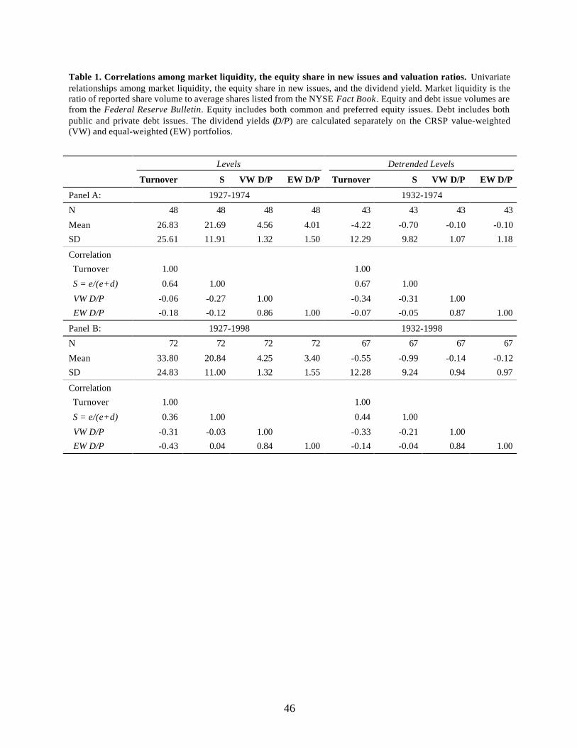
46

Table 1. Correlations among market liquidity, the equity share in new issues and valuation ratios. Univariaterelationships among market liquidity, the equity share in new issues, and the dividend yield. Market liquidity is theratio of reported share volume to average shares listed from the NYSE Fact Book . Equity and debt issue volumes arefrom the Federal Reserve Bulletin. Equity includes both common and preferred equity issues. Debt includes bothpublic and private debt issues. The dividend yields (D/P) are calculated separately on the CRSP value-weighted(VW) and equal-weighted (EW) portfolios.

Levels Detrended Levels

Turnover S VW D/P EW D/P Turnover S VW D/P EW D/P

Panel A: 1927-1974 1932-1974

N 48 48 48 48 43 43 43 43

Mean 26.83 21.69 4.56 4.01 -4.22 -0.70 -0.10 -0.10

SD 25.61 11.91 1.32 1.50 12.29 9.82 1.07 1.18

Correlation

Turnover 1.00 1.00

S = e/(e+d) 0.64 1.00 0.67 1.00

VW D/P -0.06 -0.27 1.00 -0.34 -0.31 1.00

EW D/P -0.18 -0.12 0.86 1.00 -0.07 -0.05 0.87 1.00

Panel B: 1927-1998 1932-1998

N 72 72 72 72 67 67 67 67

Mean 33.80 20.84 4.25 3.40 -0.55 -0.99 -0.14 -0.12

SD 24.83 11.00 1.32 1.55 12.28 9.24 0.94 0.97

Correlation

Turnover 1.00 1.00

S = e/(e+d) 0.36 1.00 0.44 1.00

VW D/P -0.31 -0.03 1.00 -0.33 -0.21 1.00

EW D/P -0.43 0.04 0.84 1.00 -0.14 -0.04 0.84 1.00

47

Table 2. Market liquidity and the equity share in new issues. OLS regressions of the equity share in new issueson market liquidity and valuation ratios:

ttttt

tt uRdRdRdPD

cbTurnoveraS ++++++= −−− 332211 ,

where S denotes the equity share in new issues. Equity and debt issue volumes are from the Federal ReserveBulletin . Equity includes both common and preferred equity issues. Debt includes both public and private debtissues. Market liquidity (Turnover) is the ratio of reported share volume to average shares listed from the NYSEFact Book . The dividend yield (D/P) is calculated on the CRSP value-weighted (VW) portfolio. The independentvariables are standardized within each subperiod to have unit variance. The first four columns show regressions inlevels. The second four columns show stochastically detrended results, where the prior five-year mean is subtractedfrom the current level of the dependent and independent variables. T-statistics are in braces and use two-lag Newey-West standard errors.

Levels Detrended Levels

coef [t-stat] coef [t-stat] coef [t-stat] coef [t-stat]

Panel A: 1927-1974 1932-1974

Turnover 7.68 [4.89] 9.59 [5.71] 6.61 [8.63] 6.73 [5.14]

VW D/P -1.85 [-1.26] -0.31 [-0.16]

Ret-1 2.46 [1.58] 1.37 [0.68]

Ret-2 0.79 [0.64] -0.69 [-0.41]

Ret-3 -0.36 [-0.26] -1.27 [-1.39]

N 48 46 43 43

R2 0.42 0.50 0.45 0.50

Panel B: 1927-1998 1932-1998

Turnover 4.00 [1.50] 3.30 [0.93] 4.10 [2.71] 3.84 [2.24]

VW D/P 1.55 [0.82] -0.05 [-0.04]

Ret-1 2.40 [1.78] 1.45 [1.01]

Ret-2 0.60 [0.45] -0.30 [-0.26]

Ret-3 -0.17 [-0.17] -0.03 [-0.03]

N 72 70 67 67

R2 0.13 0.12 0.20 0.22

48

Table 3. Multivariate regressions for predicting one-year-ahead market returns, 1933-1999. Regressions ofannual real equity market returns on the equity share in new issues, market liquidity, and valuation ratios:

tt

ttt uPD

dcTurnoverbSaR ++++=−

−−1

11 ,

where R denotes real percentage returns on the CRSP value-weighted (VW) or equal-weighted (EW) portfolio.Equity and debt issue volumes are from the Federal Reserve Bulletin. Equity includes both common and preferredequity issues. Debt includes both public and private debt issues. Market liquidity is the ratio of reported sharevolume to average shares listed from the NYSE Fact Book . The dividend yields (D/P) are calculated separately onthe CRSP value-weighted (VW) and equal-weighted (EW) portfolios. The independent variables are standardizedwithin each subperiod to have unit variance and stochastically detrended. We report OLS coefficients and smallsample bootstrap, bias-adjusted coefficients below. Bootstrap p-values are in brackets, and represent a two-tailed testof the null hypothesis of no predictability.

Value-Weighted Equal-Weighted

(1) (2) (3) (4) (1) (2) (3) (4)

S -7.21 -6.24 -6.11 -13.37 -8.96 -9.05

-7.25 -6.45 -6.37 -13.37 -9.09 -9.26

[0.01] [0.02] [0.02] [0.00] [0.02] [0.02]

Turnover -5.01 -2.21 -1.73 -14.07 -10.05 -9.49

-4.25 -1.33 -0.99 -12.84 -8.82 -8.42

[0.18] [0.53] [0.64] [0.02] [0.07] [0.10]

D/P 1.63 3.69

0.90 2.60

[0.54] [0.32]

N 67 67 67 67 67 67 67 67

R2 0.15 0.07 0.16 0.16 0.20 0.21 0.29 0.30