market models for predicting phev adoption and diffusion

Technical Challenges of Plug-In Hybrid Electric Vehicles and Impacts to the U.S. Power System, Subcontract No. 46827, Task 2c: Market Models for Predicting PHEV Adoption and Diffusion, Final Report

Market Models for Predicting PHEV Adoption and Diffusion

Walter McManus and Richard Senter, Jr.

University of Michigan Transportation Research Institute

2

Technical Report Documentation Page

1. Report No.

UMTRI-2009-37

2. Government Accession No. 3. Recipient’s Catalog No.

5. Report Date July 2009 4. Title and Subtitle Market Models for Predicting PHEV Adoption and Diffusion 6. Performing

Organization Code

7. Author(s) Walter McManus and Richard Senter, Jr.

8. Performing Organization Report No.

10. Work Unit no. (TRAIS)

9. Performing Organization Name and Address Automotive Analysis Division

University of Michigan Transportation Research Institute 2901 Baxter Road Ann Arbor, Michigan 48109-2150 U.S.A.

11. Contract or Grant No.

13. Type of Report and Period Covered

12. Sponsoring Agency Name and Address U.S. Department of Energy

14. Sponsoring Agency Code

15. Supplementary Notes

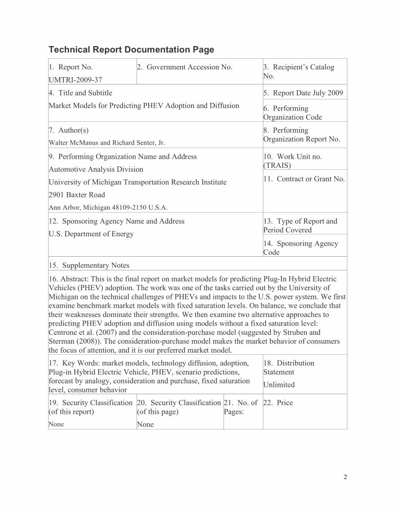
16. Abstract: This is the final report on market models for predicting Plug-In Hybrid Electric Vehicles (PHEV) adoption. The work was one of the tasks carried out by the University of Michigan on the technical challenges of PHEVs and impacts to the U.S. power system. We first examine benchmark market models with fixed saturation levels. On balance, we conclude that their weaknesses dominate their strengths. We then examine two alternative approaches to predicting PHEV adoption and diffusion using models without a fixed saturation level: Centrone et al. (2007) and the consideration-purchase model (suggested by Struben and Sterman (2008)). The consideration-purchase model makes the market behavior of consumers the focus of attention, and it is our preferred market model.

17. Key Words: market models, technology diffusion, adoption, Plug-in Hybrid Electric Vehicle, PHEV, scenario predictions, forecast by analogy, consideration and purchase, fixed saturation level, consumer behavior

18. Distribution Statement Unlimited

19. Security Classification (of this report) None

20. Security Classification (of this page) None

21. No. of Pages:

22. Price

3

Table of Contents

Market Models for Predicting PHEV Adoption and Diffusion.............................................1

Technical Report Documentation Page..................................................................................2

Table of Contents....................................................................................................................3

List of Figures .........................................................................................................................4

List of Tables...........................................................................................................................5

Introduction ............................................................................................................................6

Market and Demographic Assumptions ................................................................................8

Models with a Fixed Saturation Level....................................................................................9

The Benchmark Models.........................................................................................................9 Results with a Fixed Saturation Level.................................................................................. 13

Discussion of Results with a Fixed Saturation Level............................................................ 14

Models without a Fixed Saturation Level ............................................................................ 15

Centrone Model .................................................................................................................. 15 Consideration-Purchase Model........................................................................................... 21

Summary of Research Findings ........................................................................................... 27

Sources and References ........................................................................................................ 29

Appendix ............................................................................................................................... 30

HEV Data 1999-2008.......................................................................................................... 30 Estimated Parameters of HEV Diffusion Models ................................................................. 30

4

List of Figures Figure 1: Annual U.S. Sales of New Vehicles to Households ....................................................8 Figure 2: Benchmark Scenario Predictions of PHEV Adoptions.............................................. 13 Figure 3: Benchmark Scenario Predictions of Cumulative PHEV Adoptions........................... 14 Figure 4: Centrone Scenario Predictions of PHEV Sales ......................................................... 18 Figure 5: Centrone Scenario Prediction of Total Potentials & Adopters................................... 19 Figure 6: Centrone Scenario Adopters Share of Potentials....................................................... 20 Figure 7: Schematic Diagram of the Consideration-Purchase Model ....................................... 21 Figure 8: Survey Price Scenario Predictions of PHEV Sales ................................................... 25 Figure 9: Survey Price Scenario Predictions of PHEV Stocks ................................................. 26

5

List of Tables Table 1: Assumed Parameters of Benchmark Diffusion Models .............................................. 12 Table 2: Assumed Parameters of the Centrone Model ............................................................. 16 Table 3: Assumed Parameters of the Consideration-Purchase Model....................................... 24 Table 4: Historical HEV Data ................................................................................................. 30 Table 5: HEV Bass Model ...................................................................................................... 30 Table 6: HEV Generalized Bass Model................................................................................... 31 Table 7: HEV Logistic Model ................................................................................................. 31 Table 8: HEV Gompertz Model .............................................................................................. 31 Table 9: HEV Centrone Model................................................................................................ 32 Table 10: HEV Consideration-Purchase Model ....................................................................... 32

6

Introduction This is the final report on market models for predicting Plug-In Hybrid Electric Vehicles (PHEV) adoption. The work was one of the research tasks carried out by the University of Michigan (in cooperation with PNNL) to examine the technical challenges of and impacts to the U.S. power system.

As we seek means to protect the environment and enhance our energy security, the transportation system is a logical place to look for tools that mitigate the sector’s negative impacts on the environment (emissions of pollutants and greenhouse gases) and energy security (through its inelastic demand for oil). Converting some portion of the installed base of vehicles used for personal mobility to PHEVs is one of a number of mitigation strategies that have been proposed. Our research focused on three critical challenges to achieving conversion of a large enough portion of the installed base of vehicles to matter: technological trade offs between PHEV performance and cost; market acceptance of a switch to PHEVs; and potential negative impact of a large base of PHEVs on the reliability of the electric grid.

These challenges are closely linked. Technology defines the set of PHEVs that are technically feasible in terms of performance; design and engineering effort; and production costs. Consumer demand is strongly influenced by vehicle performance, price, and costs of operation. For a sustainable PHEV market (i.e., without government incentives in the long run) to develop, manufacturers must discover and produce the PHEV configurations that provide more value to consumers than they cost to produce and operate. The relationship between cost and value determines the ultimate market potential of PHEVs and the rate at which it is attained, which in turn determine the impact PHEVs have on demand for electricity and the reliability of the electric grid.

Our research on market acceptance involved both data collection and analytical modeling. The effort was carried out in three sub-tasks: surveying consumers to collect information on their attitudes and beliefs about PHEVs (Task 2a), simulating the dynamics of consumer adoption using a complex system model (Task 2b), and (the subject of this report) predicting the adoption and diffusion of PHEVs using market models (Task 2c). In addition to the consumer data collected by survey, additional data were collected to support the analysis of the survey and both modeling tasks.

Complex system models (or agent based models) and market models represent distinct but complementary approaches. Market models focus on predicting aggregate market-level outcomes, such as product units produced and sold, selling price, production cost, and the ultimate size of the potential market. Economic theory links the aggregate market outcomes to the underlying choice behavior of individual consumers, dealers, or other entities that participate in the market. In effect, all individual consumers are aggregated into a single “representative consumer” who is a rational economic optimizer. Agent based modeling, on the other hand, starts with agent (buyer, dealers, government) preferences and basic behavior rules and allows them to interact, thus projecting into the future and looking for collective responses (market penetration), which may or may not be optimal. The two approaches working together permit a thorough elucidation of the behavior of the players and a better sense of the likely

7

success of PHEVs in the automobile marketplace. Several considerations make predicting the adoption and diffusion of PHEVs difficult. Revealed preference data (derived from the actual market choices that consumers make) are generally the best information for generating stable and accurate forecasts. However, since PHEVs have not yet been introduced to the market (they are expected in 2010), there are no sales data to extrapolate, no PHEV owners to interview. Information collected in Task 2a [Curtin et al. (2009)] includes stated preferences for HEVs and PHEVs.

The automobile is a mature product that is deeply integrated into modern American society. The dynamic relationships between purchase, use, resale, and disposal can greatly influence the attractiveness of PHEVs to consumers and the rate of diffusion in the market.

The report is organized as follows. The common demographic and market assumptions maintained in all the prediction scenarios are described immediately following this introduction. The next section covers models with fixed saturation levels (a fixed ultimate market potential), which we refer to as “benchmark” models. We describe the benchmark models, explain our parameter assumptions, and discuss the strengths and weaknesses of the benchmark models’ prediction scenarios. On balance, we conclude that the weaknesses dominate the strengths.

Next, we present two alternative approaches to predicting PHEV adoption and diffusion using models without a fixed saturation level. Our first no-fixed-saturation-level model was presented in Centrone et al. (2007). The second model, which we refer to as the “consideration-purchase” model, was suggested by Struben & Sterman (2008). The Centrone model is in the tradition of the Bass model, in that it makes no behavioral assumptions. We attempted the same approach to predicting PHEV adoption and diffusion with the Centrone model that we used for the fixed-saturation benchmark models—parameter assumptions derived from an analysis of HEV sales 2000-08. However, the parameters and the predictions we make with them are fragile.

The consideration-purchase model, in contrast to Centrone, makes the market behavior of consumers the focus of attention. We present it as our preferred market model to predict PHEV adoption and diffusion. This allows us to enhance our market predictions by using behavioral assumptions derived from the PHEV survey reported in Curtin et al. (2009). We present these predictions and discuss describe the flexibility that we have built into the consideration-purchase model.

8

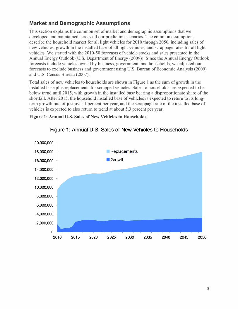
Market and Demographic Assumptions This section explains the common set of market and demographic assumptions that we developed and maintained across all our prediction scenarios. The common assumptions describe the household market for all light vehicles for 2010 through 2050, including sales of new vehicles, growth in the installed base of all light vehicles, and scrappage rates for all light vehicles. We started with the 2010-50 forecasts of vehicle stocks and sales presented in the Annual Energy Outlook (U.S. Department of Energy (2009)). Since the Annual Energy Outlook forecasts include vehicles owned by business, government, and households, we adjusted our forecasts to exclude business and government using U.S. Bureau of Economic Analysis (2009) and U.S. Census Bureau (2007). Total sales of new vehicles to households are shown in Figure 1 as the sum of growth in the installed base plus replacements for scrapped vehicles. Sales to households are expected to be below trend until 2015, with growth in the installed base bearing a disproportionate share of the shortfall. After 2015, the household installed base of vehicles is expected to return to its long-term growth rate of just over 1 percent per year, and the scrappage rate of the installed base of vehicles is expected to also return to trend at about 5.3 percent per year. Figure 1: Annual U.S. Sales of New Vehicles to Households

9

Models with a Fixed Saturation Level “Unconditional forecasts based on a data-based estimate of a fixed saturation level form a difficult benchmark to beat.” –Meade & Islam (2001)

We developed four “benchmark” models that predict the diffusion of PHEVs. They are: Bass (1969), Generalized Bass (Krishnan et al. (1999)), Logistic, and Gompertz models. All four models have a fixed saturation level, and three (Bass, Logistic, and Gompertz) generate unconditional predictions since they are one-variable functions of time. In Generalized Bass (GBass), sales depend on time, price, and the value of fuel saved; so that to predict sales one needs first to predict price and value of fuel saved. In models with a fixed saturation level, price and other variables operate to change the shape of the diffusion curve, but not the ultimate market potential.

Bass and Generalized Bass describe the diffusion of new products as the result of social interaction between users and potential users of the product. Like many economic models, Bass models predict the aggregate market outcomes with parameters estimated on aggregate data, which are then interpreted in terms of the behavior of individual consumers. It could be argued that Logistic and Gompertz are not economic models since they lack a Bass-like micro level interpretation. However, because the empirical challenge that all four benchmark models face is the same, fitting an S-shaped, or sigmoid, curve, then a micro level interpretation is a flimsy basis for preferring Bass and GBass to Logistic and Gompertz.

The Benchmark Models In this section, we describe the application of the benchmark models to predict PHEV adoption and diffusion. We developed a scenario prediction for each benchmark model (Bass, GBass, Logistic, and Gompertz) under the common set of market and demographic assumptions with assumed parameter values that we derived from an analysis of sales of HEVs for 2000-08. This method of forecasting technology adoption is called forecasting by analogy (Schnaars 2009). We assume that the situation of PHEVs with respect to adoption is similar enough to the historical situation of HEVs so that they are analogous. We also assume that the products are not so similar that they could be considered simply generations of the same product. The data and statistical estimates of the HEV adoption parameters are provided in the Appendix.

The producers (sellers) of a new product (hope they) can influence the rate at which potential users become users through the four Ps of marketing—product, price, place, and promotion. The rate at which potential users become users is also influenced by social and economic interaction between users and potential users—word-of-mouth and plainly visible (even conspicuous) consumption choices of neighbors, co-workers, and co-commuters. The four Ps are external interventions that aim to directly influence some potential users to become users. Word-of-mouth and conspicuous consumption are channels of influence that are internal parts of the social/market system.

We now explain the equations that define the benchmark models. Time, t, is defined by calendar year. We assume the first adoptions of PHEVs occur in 2010, so that t=1 in 2010. We present scenario predictions that extend through 2050 (t=49). We define A t( ) to represent the

10

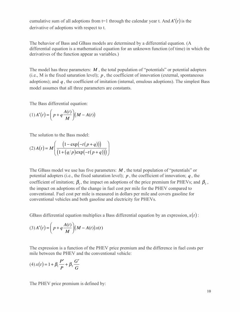
cumulative sum of all adoptions from t=1 through the calendar year t. And !A t( ) is the derivative of adoptions with respect to t. The behavior of Bass and GBass models are determined by a differential equation. (A differential equation is a mathematical equation for an unknown function (of time) in which the derivatives of the function appear as variables.)

The model has three parameters: M , the total population of “potentials” or potential adopters (i.e., M is the fixed saturation level); p , the coefficient of innovation (external, spontaneous adoptions); and q , the coefficient of imitation (internal, emulous adoptions). The simplest Bass model assumes that all three parameters are constants.

The Bass differential equation:

(1) !A t( ) = p + q A(t)M

"#$

%&'M ( A(t)( )

The solution to the Bass model:

(2)A t( ) = M1! exp !t p + q( )( )( )

1+ q p( )exp !t p + q( )( )( )"

#$

%

&'

The GBass model we use has five parameters: M , the total population of “potentials” or potential adopters (i.e., the fixed saturation level); p , the coefficient of innovation; q , the coefficient of imitation; !1 , the impact on adoptions of the price premium for PHEVs; and !2 , the impact on adoptions of the change in fuel cost per mile for the PHEV compared to conventional. Fuel cost per mile is measured in dollars per mile and covers gasoline for conventional vehicles and both gasoline and electricity for PHEVs.

GBass differential equation multiplies a Bass differential equation by an expression, x t( ) :

(3) !A t( ) = p + qA(t)M

"#$

%&'M ( A(t)( )x(t)

The expression is a function of the PHEV price premium and the difference in fuel costs per mile between the PHEV and the conventional vehicle:

(4) x t( ) = 1+ !1"PP

+ !2"G

G

The PHEV price premium is defined by:

11

(5)P t( ) = price of PHEV ! price of conventionalprice of conventional

The difference in cost per mile is defined by:

(6)G t( ) = cpm1 ! cpm0

Cost per mile is defined for each vehicle type (n=0 for conventional and n=1 for PHEV):

(7)cpmn =price of fuel in cents per unit

miles per unit of fuel

The solution to the GBass model:

(8)A t( ) = M1! exp ! p + q( ) t + "1 ln P t( )( ) + "2 ln G t( )( )( )( )

1+ q p( )exp ! p + q( ) t + "1 ln P t( )( ) + "2 ln G t( )( )( )( )#

$%%

&

'((

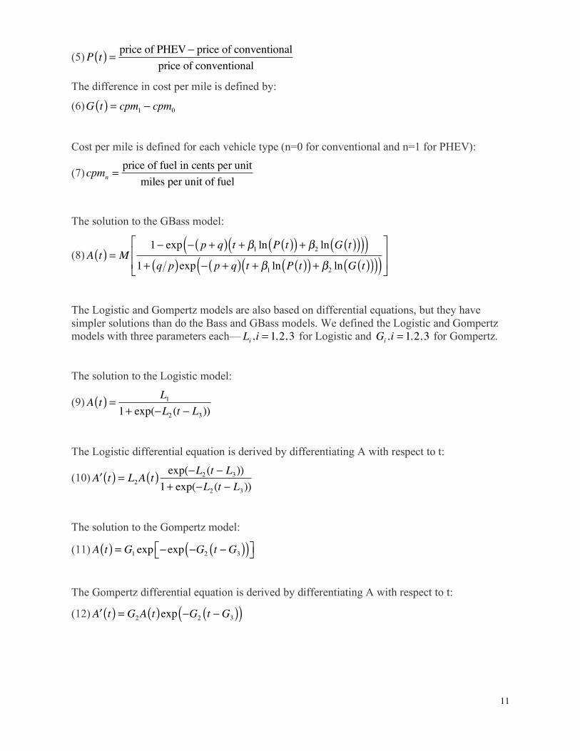
The Logistic and Gompertz models are also based on differential equations, but they have simpler solutions than do the Bass and GBass models. We defined the Logistic and Gompertz models with three parameters each— Li ,i = 1,2,3 for Logistic and Gi ,i = 1,2,3 for Gompertz.

The solution to the Logistic model:

(9)A t( ) = L11+ exp(!L2 (t ! L3))

The Logistic differential equation is derived by differentiating A with respect to t:

(10) !A t( ) = L2A t( ) exp("L2 (t " L3))1+ exp("L2 (t " L3))

The solution to the Gompertz model:

(11)A t( ) = G1 exp ! exp !G2 t !G3( )( )"# $%

The Gompertz differential equation is derived by differentiating A with respect to t:

(12) !A t( ) = G2A t( )exp "G2 t "G3( )( )

12

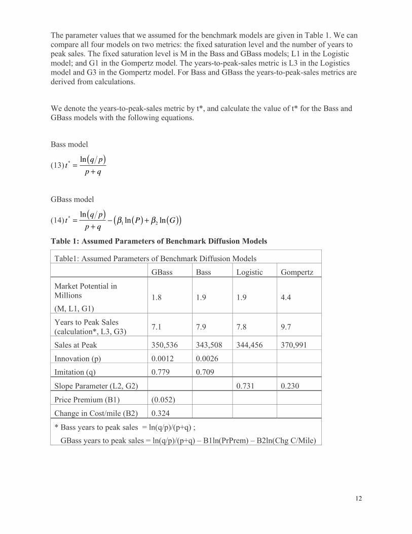
The parameter values that we assumed for the benchmark models are given in Table 1. We can compare all four models on two metrics: the fixed saturation level and the number of years to peak sales. The fixed saturation level is M in the Bass and GBass models; L1 in the Logistic model; and G1 in the Gompertz model. The years-to-peak-sales metric is L3 in the Logistics model and G3 in the Gompertz model. For Bass and GBass the years-to-peak-sales metrics are derived from calculations.

We denote the years-to-peak-sales metric by t*, and calculate the value of t* for the Bass and GBass models with the following equations.

Bass model

(13) t* =ln q p( )p + q

GBass model

(14) t* =ln q p( )p + q

! "1 ln P( ) + "2 ln G( )( )

Table 1: Assumed Parameters of Benchmark Diffusion Models

Table1: Assumed Parameters of Benchmark Diffusion Models

GBass Bass Logistic Gompertz

Market Potential in Millions (M, L1, G1)

1.8 1.9 1.9 4.4

Years to Peak Sales (calculation*, L3, G3) 7.1 7.9 7.8 9.7

Sales at Peak 350,536 343,508 344,456 370,991

Innovation (p) 0.0012 0.0026

Imitation (q) 0.779 0.709

Slope Parameter (L2, G2) 0.731 0.230

Price Premium (B1) (0.052)

Change in Cost/mile (B2) 0.324

* Bass years to peak sales = ln(q/p)/(p+q) ; GBass years to peak sales = ln(q/p)/(p+q) – B1ln(PrPrem) – B2ln(Chg C/Mile)

13

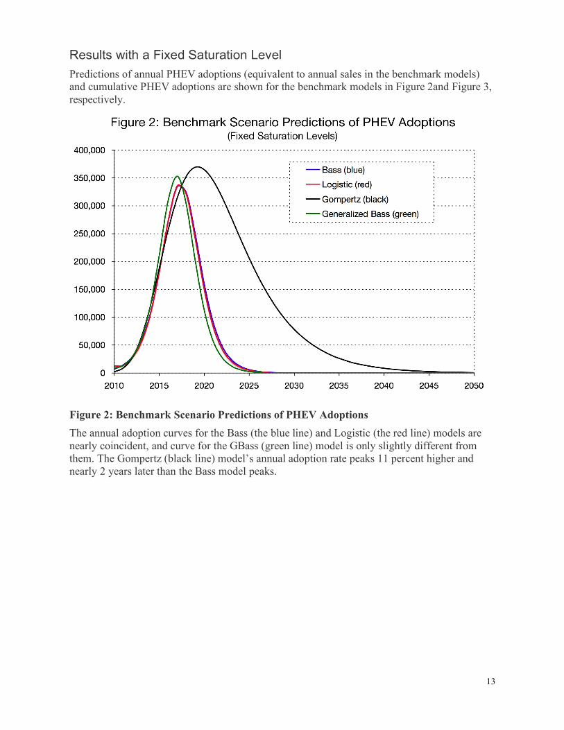
Results with a Fixed Saturation Level Predictions of annual PHEV adoptions (equivalent to annual sales in the benchmark models) and cumulative PHEV adoptions are shown for the benchmark models in Figure 2and Figure 3, respectively.

Figure 2: Benchmark Scenario Predictions of PHEV Adoptions The annual adoption curves for the Bass (the blue line) and Logistic (the red line) models are nearly coincident, and curve for the GBass (green line) model is only slightly different from them. The Gompertz (black line) model’s annual adoption rate peaks 11 percent higher and nearly 2 years later than the Bass model peaks.

14

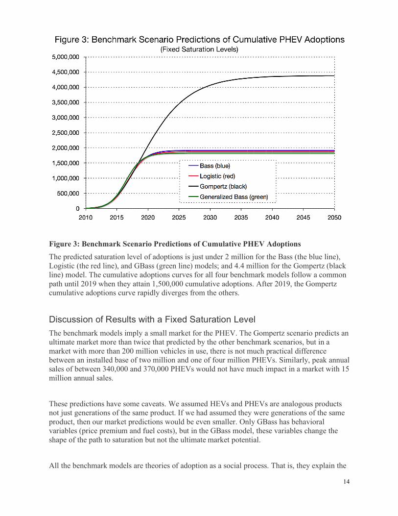
Figure 3: Benchmark Scenario Predictions of Cumulative PHEV Adoptions The predicted saturation level of adoptions is just under 2 million for the Bass (the blue line), Logistic (the red line), and GBass (green line) models; and 4.4 million for the Gompertz (black line) model. The cumulative adoptions curves for all four benchmark models follow a common path until 2019 when they attain 1,500,000 cumulative adoptions. After 2019, the Gompertz cumulative adoptions curve rapidly diverges from the others.

Discussion of Results with a Fixed Saturation Level The benchmark models imply a small market for the PHEV. The Gompertz scenario predicts an ultimate market more than twice that predicted by the other benchmark scenarios, but in a market with more than 200 million vehicles in use, there is not much practical difference between an installed base of two million and one of four million PHEVs. Similarly, peak annual sales of between 340,000 and 370,000 PHEVs would not have much impact in a market with 15 million annual sales.

These predictions have some caveats. We assumed HEVs and PHEVs are analogous products not just generations of the same product. If we had assumed they were generations of the same product, then our market predictions would be even smaller. Only GBass has behavioral variables (price premium and fuel costs), but in the GBass model, these variables change the shape of the path to saturation but not the ultimate market potential.

All the benchmark models are theories of adoption as a social process. That is, they explain the

15

movement of consumers from the potential social group to the adopter social group. However, the models are usually estimated using sales and cumulative sales, ignoring both replacement purchases of the new product technology by past adopters and defections by past adopters to the old technology. In the first few years after the new technology is introduced, this approach is accurate since the vast majority of sales are likely to be first-time adoptions. However, as the market matures, sales include a growing fraction of replacements by prior adopters, and the rate of adoption is overstated.

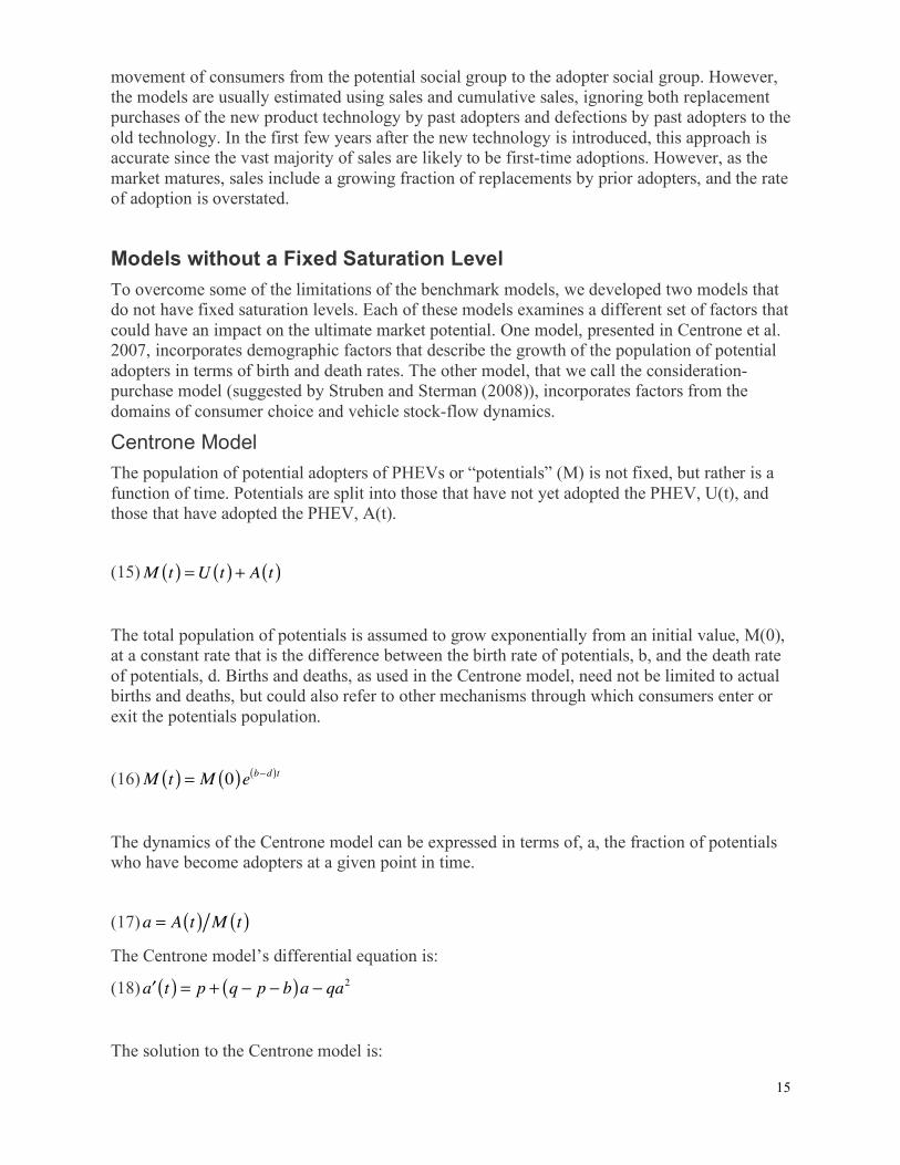
Models without a Fixed Saturation Level To overcome some of the limitations of the benchmark models, we developed two models that do not have fixed saturation levels. Each of these models examines a different set of factors that could have an impact on the ultimate market potential. One model, presented in Centrone et al. 2007, incorporates demographic factors that describe the growth of the population of potential adopters in terms of birth and death rates. The other model, that we call the consideration-purchase model (suggested by Struben and Sterman (2008)), incorporates factors from the domains of consumer choice and vehicle stock-flow dynamics.

Centrone Model The population of potential adopters of PHEVs or “potentials” (M) is not fixed, but rather is a function of time. Potentials are split into those that have not yet adopted the PHEV, U(t), and those that have adopted the PHEV, A(t).

(15)M t( ) =U t( ) + A t( )

The total population of potentials is assumed to grow exponentially from an initial value, M(0), at a constant rate that is the difference between the birth rate of potentials, b, and the death rate of potentials, d. Births and deaths, as used in the Centrone model, need not be limited to actual births and deaths, but could also refer to other mechanisms through which consumers enter or exit the potentials population.

(16)M t( ) = M 0( )e b!d( )t

The dynamics of the Centrone model can be expressed in terms of, a, the fraction of potentials who have become adopters at a given point in time.

(17)a = A t( ) M t( )

The Centrone model’s differential equation is:

(18) !a t( ) = p + q " p " b( )a " qa2

The solution to the Centrone model is:

16

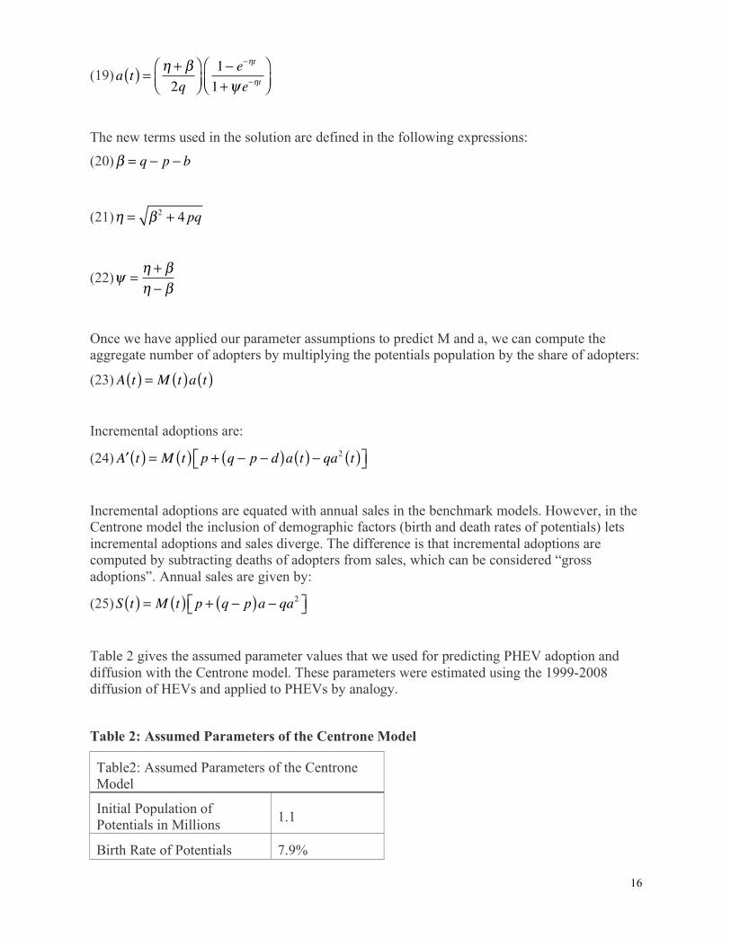
(19)a t( ) = ! + "2q

#$%

&'(

1) e)!t

1+* e)!t#$%

&'(

The new terms used in the solution are defined in the following expressions:

(20)! = q " p " b

(21)! = " 2 + 4 pq

(22)! =" + #" $ #

Once we have applied our parameter assumptions to predict M and a, we can compute the aggregate number of adopters by multiplying the potentials population by the share of adopters:

(23)A t( ) = M t( )a t( )

Incremental adoptions are:

(24) !A t( ) = M t( ) p + q " p " d( )a t( ) " qa2 t( )#$ %&

Incremental adoptions are equated with annual sales in the benchmark models. However, in the Centrone model the inclusion of demographic factors (birth and death rates of potentials) lets incremental adoptions and sales diverge. The difference is that incremental adoptions are computed by subtracting deaths of adopters from sales, which can be considered “gross adoptions”. Annual sales are given by:

(25)S t( ) = M t( ) p + q ! p( )a ! qa2"# $%

Table 2 gives the assumed parameter values that we used for predicting PHEV adoption and diffusion with the Centrone model. These parameters were estimated using the 1999-2008 diffusion of HEVs and applied to PHEVs by analogy.

Table 2: Assumed Parameters of the Centrone Model

Table2: Assumed Parameters of the Centrone Model

Initial Population of Potentials in Millions 1.1

Birth Rate of Potentials 7.9%

17

Death Rate of Potentials 0.000000151%

Innovation (p) 0.00259

Imitation (q) 0.62029

18

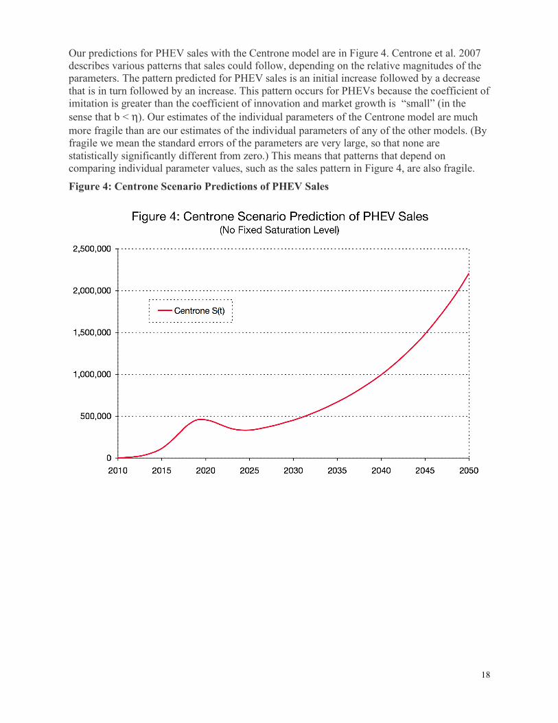
Our predictions for PHEV sales with the Centrone model are in Figure 4. Centrone et al. 2007 describes various patterns that sales could follow, depending on the relative magnitudes of the parameters. The pattern predicted for PHEV sales is an initial increase followed by a decrease that is in turn followed by an increase. This pattern occurs for PHEVs because the coefficient of imitation is greater than the coefficient of innovation and market growth is “small” (in the sense that b < η). Our estimates of the individual parameters of the Centrone model are much more fragile than are our estimates of the individual parameters of any of the other models. (By fragile we mean the standard errors of the parameters are very large, so that none are statistically significantly different from zero.) This means that patterns that depend on comparing individual parameter values, such as the sales pattern in Figure 4, are also fragile.

Figure 4: Centrone Scenario Predictions of PHEV Sales

19

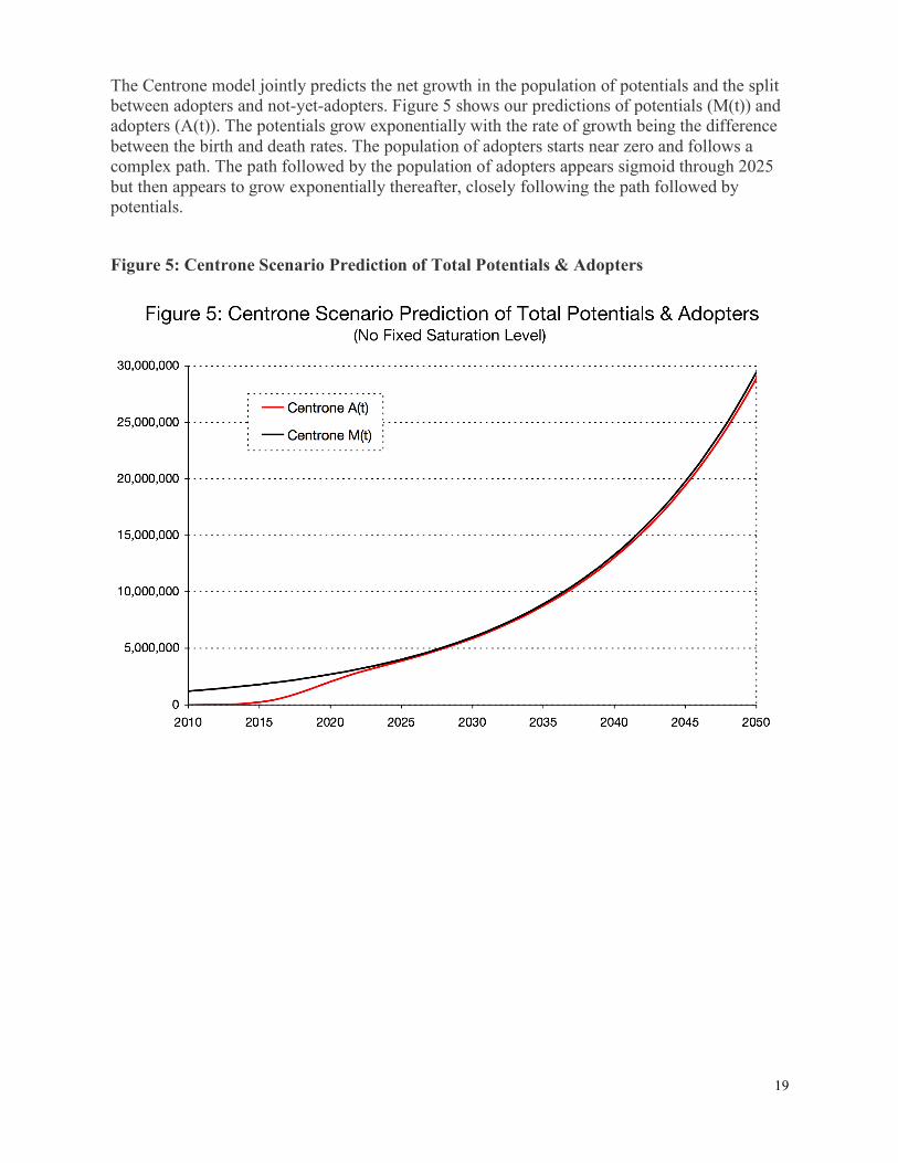
The Centrone model jointly predicts the net growth in the population of potentials and the split between adopters and not-yet-adopters. Figure 5 shows our predictions of potentials (M(t)) and adopters (A(t)). The potentials grow exponentially with the rate of growth being the difference between the birth and death rates. The population of adopters starts near zero and follows a complex path. The path followed by the population of adopters appears sigmoid through 2025 but then appears to grow exponentially thereafter, closely following the path followed by potentials.

Figure 5: Centrone Scenario Prediction of Total Potentials & Adopters

20

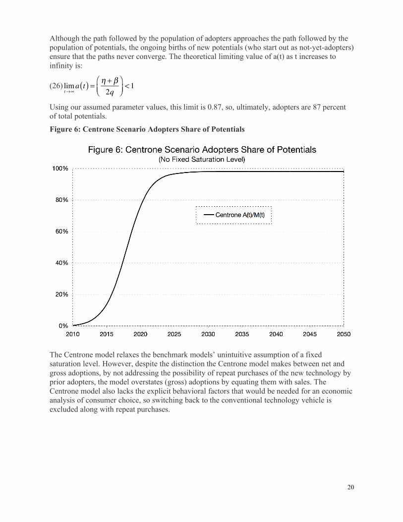
Although the path followed by the population of adopters approaches the path followed by the population of potentials, the ongoing births of new potentials (who start out as not-yet-adopters) ensure that the paths never converge. The theoretical limiting value of a(t) as t increases to infinity is:

(26) limt!"

a t( ) = # + $2q

%&'

()*< 1

Using our assumed parameter values, this limit is 0.87, so, ultimately, adopters are 87 percent of total potentials.

Figure 6: Centrone Scenario Adopters Share of Potentials

The Centrone model relaxes the benchmark models’ unintuitive assumption of a fixed saturation level. However, despite the distinction the Centrone model makes between net and gross adoptions, by not addressing the possibility of repeat purchases of the new technology by prior adopters, the model overstates (gross) adoptions by equating them with sales. The Centrone model also lacks the explicit behavioral factors that would be needed for an economic analysis of consumer choice, so switching back to the conventional technology vehicle is excluded along with repeat purchases.

21

Consideration-Purchase Model We developed the consideration-purchase model (suggested in Struben and Sterman (2008)) to build on the strengths of the benchmark and Centrone models, while overcoming some of their limitations. The model explicitly incorporates a consumer choice component that can be expanded well beyond its current simplified form. The highly simplified form was chosen to match the “choice experiment” in the PHEV survey (Curtin et al. 2009). The model also accounts for the dynamics of vehicle sales, stock, and scrappage.

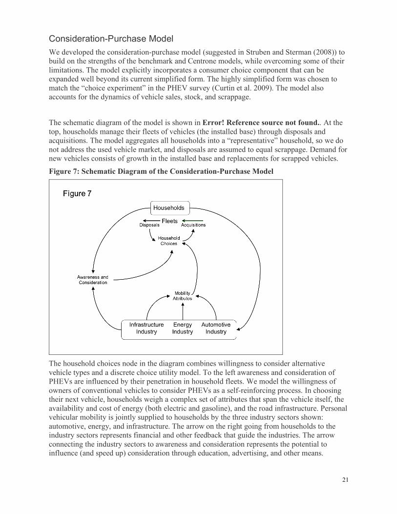
The schematic diagram of the model is shown in Error! Reference source not found.. At the top, households manage their fleets of vehicles (the installed base) through disposals and acquisitions. The model aggregates all households into a “representative” household, so we do not address the used vehicle market, and disposals are assumed to equal scrappage. Demand for new vehicles consists of growth in the installed base and replacements for scrapped vehicles.

Figure 7: Schematic Diagram of the Consideration-Purchase Model

The household choices node in the diagram combines willingness to consider alternative vehicle types and a discrete choice utility model. To the left awareness and consideration of PHEVs are influenced by their penetration in household fleets. We model the willingness of owners of conventional vehicles to consider PHEVs as a self-reinforcing process. In choosing their next vehicle, households weigh a complex set of attributes that span the vehicle itself, the availability and cost of energy (both electric and gasoline), and the road infrastructure. Personal vehicular mobility is jointly supplied to households by the three industry sectors shown: automotive, energy, and infrastructure. The arrow on the right going from households to the industry sectors represents financial and other feedback that guide the industries. The arrow connecting the industry sectors to awareness and consideration represents the potential to influence (and speed up) consideration through education, advertising, and other means.

22

Mathematically, the consideration-purchase model is contained in a set of equations, (27) through (32). The dynamics of the household fleets are defined in (27). The total installed base of household vehicles, V, consists of two types: conventional vehicles, V0, and PHEVs, V1. The annual growth in the total installed base is derived from our market and demographic assumptions (Figure 1). We split total growth between V0 and V1 in proportion to their share of the total stock. The disposal rate of conventional vehicles is close to the overall total stock rate (5.3%), reflecting the maturity of the conventional products. The disposal rate for PHEVs is assumed to start at zero with the launch, and to gradually rise toward the 5.3% overall rate as the PHEV market matures.

Overall vehicle dynamics:

(27)Vt = V0,t +V1,tVt = Vt!1 + " t( )Vt!1 ! #0 t( )V0,t!1 ! #1 t( )V1,t!1

For each of the vehicle types, the installed base in period t is equal to the installed base of the same type in period t-1, minus scrappage of the same type, plus new sales of the same type.

Dynamics of V0 and V1

(28)V0,t = V0,t!1 ! "0 t( )V0,t!1 + S0,tV1,t = V1,t!1 ! "1 t( )V1,t!1 + S1,t

Market demand for new vehicles consists of customers in four situations: replacing a conventional vehicle (V0 owners), replacing a PHEV (V1 owners), adding a vehicle to an all-conventional fleet, and adding a vehicle to an all-PHEV fleet. [This is an attempt at a simple explanation. What we are doing is splitting overall fleet growth between V0 and V1 in the same ratio as V1 and V0 are to each other in the installed base.] The δ parameters are scrappage rates, the γ parameters are growth rates, and ∏ij is the probability that an i-owner buys a j-vehicle (whether replacement or growth) conditional on the i-owner’s willingness to consider the j-vehicle. We assume (following Struben and Sterman (2008)) that all consumers consider the conventional vehicle, and that all PHEV owners returning to the new-vehicle market consider a PHEV replacement purchase.

Sales equations

(29)S0,t = !00 "0 t( )V0,t#1 +!10 "1 t( )V1,t#1 +!00 $ t( )V0,t#1 +!10 $ t( )V1,t#1S1,t = !01"0 t( )V0,t#1 +!11"1 t( )V1,t#1 +!01 $ t( )V0,t#1 +!11 $ t( )V1,t#1

The discrete choice probabilities for PHEV (V1) owners are functions of the relative utilities only (with u0=0), since all PHEV (V1) owners are assumed to consider both PHEV (V1) and conventional (V0).

23

(30)!11 =

exp u1( )1+ exp u1( )

!10 = 1" !11 =1

1+ exp u1( )

The discrete choice probabilities for conventional (V0) owners are functions of the relative utilities and the willingness to consider the PHEV (V1), w(t) ≤ 1.

(31)

!00 = 1" !01 =1

1+ w t( )exp u1( )

!01 =w t( )exp u1( )

1+ w t( )exp u1( )

We apply a Bass-type model to describe the dynamic behavior of the willingness of owners of conventional vehicles to consider the PHEV. The differential equation and the solution are familiar.

The differential equation:

!w t( ) = a + bw( ) 1" w( )

The solution:

(32)w t( ) = 1! e! a+b( )t

1+ b a( )e! a+b( )t

For a given price, the consideration-purchase model has three parameters: the coefficient of innovation in the willingness of conventional owners to consider the PHEV (a), the coefficient of imitation in the willingness of conventional owners to consider the PHEV (b), and the exponential utility of the PHEV (exp(u1)). We assume that exp(u1) is the same for all consumer, whether they are conventional owners or PHEV owners.

24

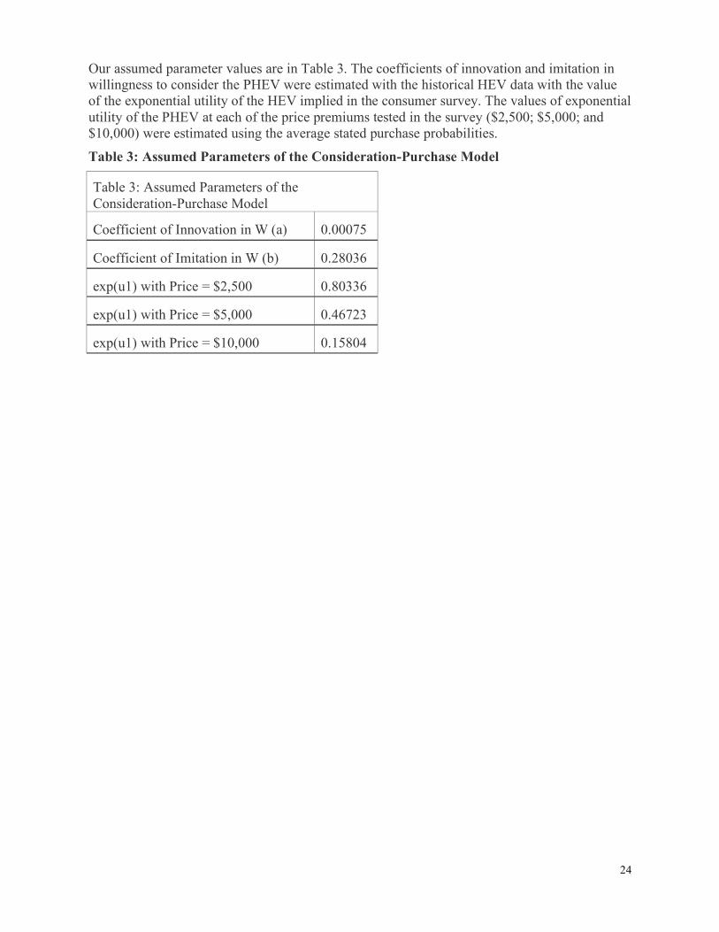
Our assumed parameter values are in Table 3. The coefficients of innovation and imitation in willingness to consider the PHEV were estimated with the historical HEV data with the value of the exponential utility of the HEV implied in the consumer survey. The values of exponential utility of the PHEV at each of the price premiums tested in the survey ($2,500; $5,000; and $10,000) were estimated using the average stated purchase probabilities.

Table 3: Assumed Parameters of the Consideration-Purchase Model

Table 3: Assumed Parameters of the Consideration-Purchase Model

Coefficient of Innovation in W (a) 0.00075

Coefficient of Imitation in W (b) 0.28036

exp(u1) with Price = $2,500 0.80336

exp(u1) with Price = $5,000 0.46723

exp(u1) with Price = $10,000 0.15804

25

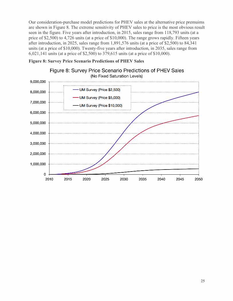
Our consideration-purchase model predictions for PHEV sales at the alternative price premuims are shown in Figure 8. The extreme sensitivity of PHEV sales to price is the most obvious result seen in the figure. Five years after introduction, in 2015, sales range from 118,793 units (at a price of $2,500) to 4,726 units (at a price of $10,000). The range grows rapidly. Fifteen years after introduction, in 2025, sales range from 1,891,576 units (at a price of $2,500) to 84,341 units (at a price of $10,000). Twenty-five years after introduction, in 2035, sales range from 6,021,141 units (at a price of $2,500) to 379,615 units (at a price of $10,000).

Figure 8: Survey Price Scenario Predictions of PHEV Sales

26

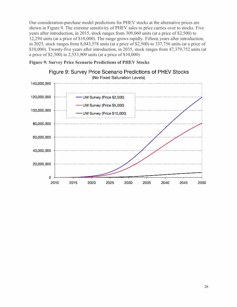
Our consideration-purchase model predictions for PHEV stocks at the alternative prices are shown in Figure 9. The extreme sensitivity of PHEV sales to price carries over to stocks. Five years after introduction, in 2015, stock ranges from 309,060 units (at a price of $2,500) to 12,294 units (at a price of $10,000). The range grows rapidly. Fifteen years after introduction, in 2025, stock ranges from 8,043,578 units (at a price of $2,500) to 337,756 units (at a price of $10,000). Twenty-five years after introduction, in 2035, stock ranges from 47,379,752 units (at a price of $2,500) to 2,533,909 units (at a price of $10,000).

Figure 9: Survey Price Scenario Predictions of PHEV Stocks

27

Summary of Research Findings In this study, we examined predictions of PHEV adoption and diffusion derived from six market models. Four models assumed fixed saturation levels and were used as benchmarks: Bass, Generalized Bass, Logistic, and Gompertz. One model used demographic factors to describe growth in market potential in terms of births and deaths of the population of potential adopters: Centrone. Our preferred model used factors related to consumer consideration and purchase choice; and factors related to vehicle stocks and flows to describe PHEV adoption and diffusion as a complex dynamic system. The predicted annual adoptions for the Bass, GBass, and Logistic models are very similar. Peak sales of roughly 350,000 are predicted to occur 7 to 8 years after introduction. The Gompertz model’s annual adoptions peak 11 percent higher and nearly 2 years later than the Bass model.

The predicted saturation level of adoptions is just under 2 million for the Bass, Logistic, and GBass models; and 4.4 million for the Gompertz model. The benchmark models track very closely for the first 9 years after introduction, attaining 1.5 million cumulative adoptions. Thereafter, the Gompertz cumulative adoptions curve rapidly diverges from the others.

The benchmark models imply a small market for the PHEV. The Gompertz scenario predicts an ultimate market more than twice that predicted by the other benchmark scenarios, but in a market with more than 200 million vehicles in use, there is not much practical difference between an installed base of two million and one of four million PHEVs. Similarly, peak annual sales of between 340,000 and 370,000 PHEVs would not have much impact in a market with 15 million annual sales. These predictions have some caveats. We assumed HEVs and PHEVs are analogous products not just generations of the same product. If we had assumed they were generations of the same product, then our market predictions would be even smaller. Only GBass has behavioral variables (price premium and fuel costs), but in the GBass model, these variables change the shape of the path to saturation but not the ultimate market potential.

To overcome some of the limitations of the benchmark models, we developed two models that do not have fixed saturation levels. Each of these models examines a different set of factors that could have an impact on the ultimate market potential. One model, presented in Centrone et al. 2007, incorporates demographic factors that describe the growth of the population of potential adopters in terms of birth and death rates. The other model, that we call the consideration-purchase model (suggested by Struben and Sterman (2008)), incorporates factors from the domains of consumer choice and vehicle stock-flow dynamics. Incremental adoptions are equated with annual sales in the benchmark models. However, in the Centrone model the inclusion of demographic factors (birth and death rates of potentials) lets incremental adoptions and sales diverge. The difference is that incremental adoptions are computed by subtracting deaths of adopters from sales, which can be considered “gross adoptions”.

The pattern predicted for PHEV sales by the Centrone model is an initial increase followed by a decrease that is in turn followed by an increase. This pattern occurs for PHEVs because the coefficient of imitation is greater than the coefficient of innovation and market growth is relatively small. The Centrone model predicts annual sales to remain under 500,000 units for 20 years after introduction, and to subsequently grow more rapidly. Sales of 1,000,000 per year are predicted 30 years after introduction, and sales of more than 2,000,000 per year are predicted 40 years after introduction.

28

The population of potentials grows exponentially at just under 8 percent per year. The population of adopters starts near zero and grows to a maximum of 87 percent of the population of potentials by 12 to 14 years after introduction.

The Centrone model relaxes the benchmark models’ unintuitive assumption of a fixed saturation level. However, despite the distinction the Centrone model makes between net and gross adoptions, by not addressing the possibility of repeat purchases of the new technology by prior adopters, the model overstates (gross) adoptions by equating them with sales. The Centrone model also lacks the explicit behavioral factors that would be needed for an economic analysis of consumer choice, so switching back to the conventional technology vehicle is excluded along with repeat purchases. We developed the consideration-purchase model (suggested in Struben and Sterman (2008)) to build on the strengths of the benchmark and Centrone models, while overcoming some of their limitations. The model explicitly incorporates a consumer choice component that can be expanded well beyond its current simplified form. The highly simplified form was chosen to match the “choice experiment” in the PHEV survey (Curtin et al. 2009). The model also accounts for the dynamics of vehicle sales, stock, and scrappage. Our consideration-purchase model predictions for PHEV sales are extremely sensitive to price premiums. Five years after introduction, in 2015, sales range from 118,793 units (at a price of $2,500) to 4,726 units (at a price of $10,000). The range grows rapidly. Fifteen years after introduction, in 2025, sales range from 1,891,576 units (at a price of $2,500) to 84,341 units (at a price of $10,000). Twenty-five years after introduction, in 2035, sales range from 6,021,141 units (at a price of $2,500) to 379,615 units (at a price of $10,000). The extreme sensitivity of PHEV sales to price premiums carries over to stocks. Five years after introduction, in 2015, stock ranges from 309,060 units (at a price of $2,500) to 12,294 units (at a price of $10,000). The range grows rapidly. Fifteen years after introduction, in 2025, stock ranges from 8,043,578 units (at a price of $2,500) to 337,756 units (at a price of $10,000). Tewnty-five years after introduction, in 2035, stock ranges from 47,379,752 units (at a price of $2,500) to 2,533,909 units (at a price of $10,000).

29

Sources and References Bass, F.M. (1969). A new product growth for model consumer durables, Manage. Sci. 15(5) 215–227.

Centrone, F., Goia, A., Salinelli, E. (2007) Demographic processes in a model of innovation diffusion with a dynamic market, Technological Forecasting & Social Change 74 247 - 266

Curtin, R., Shrago, Y., and Mikkelsen, J. (2009). Plug-in Hybrid Electric Vehicles. Ann Arbor, MI: University of Michigan.

Dodson, J.A. and Muller, E. (1978) Models of new product diffusion through advertising and word-of-mouth, Manage. Sci. 24(15) 1568–1578.

Horsky, D. (1990) A diffusion model incorporating product benefits, price, income and information, Mark. Sci. 9(4) 342–365.

Jain, D.C. and Rao, R.C. (1990) Effect of price on the demand for durables: modeling, estimation and findings, J. Bus. Econ. Stat. 8(2) 163–170.

Krishnan, T.V., Bass, F.M. Bass, and Jain, D.C. (1999). Optimal Pricing Strategy for New Products, Management Science, v.45 n.12, p.1650-1663.

Mahajan, and Muller, V. E. (1979) Innovation diffusion and new product growth models in marketing, J. Mark. 43(4) 55–68. Meade, N, and Islam, T. (2001). Forecasting the diffusion of innovations: implications for time series extrapolation. In J.S. Armstrong (Ed.), Principles of forecasting: A handbook for researchers and practitioners (pp. 577-595). Norwell, MA: Kluwer Academic Publishers.

Schnaars, S. 2009. Forecasting the future of technology by analogy—An evaluation of two prominent cases from the 20th century. Technology in Society 31(2) 187-195.

StataCorp. 2007. Stata Statistical Software: Release 10. College Station, TX: StataCorp LP. Struben, J. and Sterman, J. (2008). Transition Challenges for Alternative Fuel Vehicle and Transportation Systems. Environment and Planning B. 35(6) 1070-1097 U.S. Bureau of Economic Analysis (2009). National Economic Accounts, Underlying Detail Table 7.2.5S. Auto and Truck Unit Sales, Production, Inventories, Expenditures, and Price Revised on June 26, 2009 Next Release Date August 07, 2009.

U.S. Census Bureau (2007). Statistical Abstract of the United States: 2007, 127th edn. Washington DC: Department of Commerce.

U.S. Department of Energy (2009). Annual Energy Outlook 2009, Report #:DOE/EIA-0383(2009) Release date full report: March 2009. Next release date full report: February 2010.

30

Appendix HEV Data 1999-2008 Table 4: Historical HEV Data

Historical Hybrid Electric Vehicle (HEV) Data

Year HEV Sales

Cumulative HEV Sales

Total Household Vehicle Sales

Price Premium

Reduction in Cost per Mile ($)

1999 0 0 12,880,000 0.0% 0.000

2000 9,367 9,367 13,234,000 4.4% 0.043

2001 20,282 29,649 13,062,000 4.4% 0.031

2002 36,035 65,684 12,831,000 4.4% 0.029

2003 47,600 113,284 12,699,000 4.4% 0.032

2004 84,199 197,483 12,869,000 4.5% 0.038

2005 209,711 407,194 12,932,000 4.5% 0.047

2006 252,636 659,830 12,593,000 22.2% 0.049

2007 352,274 1,012,104 11,662,000 22.2% 0.050

2008 312,386 1,324,490 9,545,000 22.2% 0.055

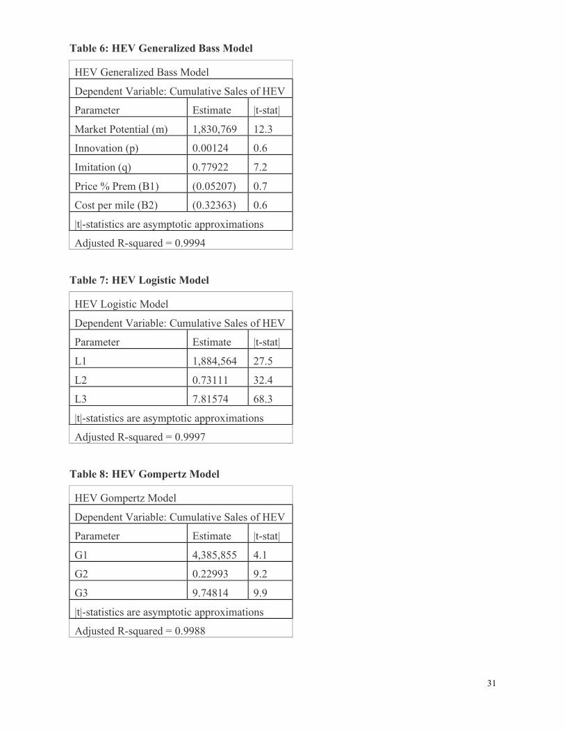
Estimated Parameters of HEV Diffusion Models The tables below present the results of our statistical analysis. The parameters of the models were estimated by nonlinear regression using HEV historical data for 1999-2008. We used statistical software from StataCorp. 2007.

Table 5: HEV Bass Model

HEV Bass Model

Dependent Variable: Cumulative Sales of HEV

Parameter Estimate |t-stat|

Market Potential (m) 1,922,806 21.1

Innovation (p) 0.00262 10.2

Imitation (q) 0.70935 24.4

|t|-statistics are asymptotic approximations

Adjusted R-squared = 0.9996

31

Table 6: HEV Generalized Bass Model

HEV Generalized Bass Model



Market Potential (m) 1,830,769 12.3

Innovation (p) 0.00124 0.6

Imitation (q) 0.77922 7.2

Price % Prem (B1) (0.05207) 0.7

Cost per mile (B2) (0.32363) 0.6



Table 7: HEV Logistic Model

HEV Logistic Model



L1 1,884,564 27.5

L2 0.73111 32.4

L3 7.81574 68.3



Table 8: HEV Gompertz Model

HEV Gompertz Model



G1 4,385,855 4.1

G2 0.22993 9.2

G3 9.74814 9.9



32

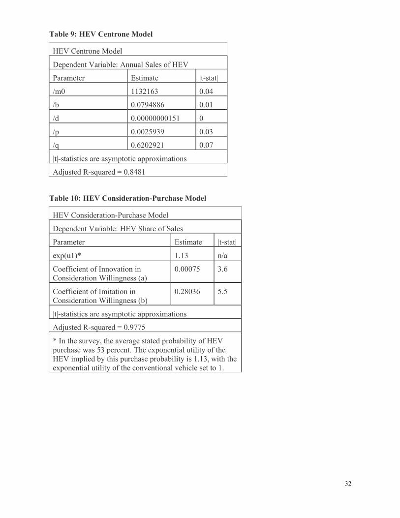
Table 9: HEV Centrone Model

HEV Centrone Model

Dependent Variable: Annual Sales of HEV


/m0 1132163 0.04

/b 0.0794886 0.01

/d 0.00000000151 0

/p 0.0025939 0.03

/q 0.6202921 0.07



Table 10: HEV Consideration-Purchase Model

HEV Consideration-Purchase Model

Dependent Variable: HEV Share of Sales


exp(u1)* 1.13 n/a

Coefficient of Innovation in Consideration Willingness (a)

0.00075 3.6

Coefficient of Imitation in Consideration Willingness (b)

0.28036 5.5



* In the survey, the average stated probability of HEV purchase was 53 percent. The exponential utility of the HEV implied by this purchase probability is 1.13, with the exponential utility of the conventional vehicle set to 1.

market models for predicting phev adoption and diffusion

Documents