Research Division Federal Reserve Bank of St. Louis Working Paper Series

Market Timing with Aggregate and Idiosyncratic Stock Volatilities

Hui Guo and

Jason Higbee

Working Paper 2005-073B http://research.stlouisfed.org/wp/2005/2005-073.pdf

December 2005 Revised February 2006

FEDERAL RESERVE BANK OF ST. LOUIS Research Division

P.O. Box 442 St. Louis, MO 63166

______________________________________________________________________________________

The views expressed are those of the individual authors and do not necessarily reflect official positions of the Federal Reserve Bank of St. Louis, the Federal Reserve System, or the Board of Governors.

Federal Reserve Bank of St. Louis Working Papers are preliminary materials circulated to stimulate discussion and critical comment. References in publications to Federal Reserve Bank of St. Louis Working Papers (other than an acknowledgment that the writer has had access to unpublished material) should be cleared with the author or authors.

Market Timing with Aggregate and Idiosyncratic Stock Volatilities

Hui Guo Jason Higbee

This Version: January 18, 2006

Hui Guo is senior economist and Jason Higbee is a senior research associate at the Federal Reserve Bank of St. Louis. Please address correspondence to Hui Guo, Research Division, Federal Reserve Bank of St. Louis, P.O. Box 442, St. Louis, MO, 63166; Hui.Guo@stls.frb.org; Phone (314) 444-8717; Fax (314) 444-8731. We especially thank an anonymous referee for many detailed and constructive comments, which greatly improved the paper. The views expressed in this paper are those of the authors and do not necessarily reflect the official positions of the Federal Reserve Bank of St. Louis or the Federal Reserve System.

1

Abstract

Guo and Savickas [2005] show that aggregate stock market volatility and average

idiosyncratic stock volatility jointly forecast stock returns. In this paper, we quantify the

economic significance of their results from the perspective of a portfolio manager. That

is, we evaluate the performance, e.g., the Sharpe ratio and Jensen’s alpha, of a mean-

variance manager who tries to time the market based on those two variables. We find

that, over the period 1968-2004, the associated market-timing strategy outperforms the

buy-and-hold strategy, and the difference is statistically and economically significant.

Keywords: Stock return predictability, CAPM, ICAPM, Idiosyncratic Volatility, Stock

Market volatility.

JEF number: G1.

2

Economic theories, e.g., Merton’s (1973) intertemporal capital asset pricing

model (ICAPM), suggest that risk-averse investors require a higher excess stock market

return when volatility increases.1 Early authors (e.g., French, Schwert, and Stambaugh

[1987]), however, find that realized stock market variance, MV, has negligible

forecasting power for returns. In a recent study, Guo and Savickas [2005] show that the

effect of MV becomes significantly positive after including realized idiosyncratic stock

variance, IV, as an additional predictor. Also, IV is found to have significantly negative

effects on returns, although it is positively correlated with MV. Their results suggest that

early authors fail to uncover a positive risk-return tradeoff possibly because of a classic

omitted variables problem: The coefficient of MV is downward biased if we do not

control for IV.

IV is constructed as the value-weighted cross-sectional average of variance of

stock price movements that are not explained by known systematic risk—for example, as

captured by the capital asset pricing model (CAPM) or the Fama and French [1993] 3-

factor model. That is, IV is a measure of average variations in stock prices that are driven

only by firm-specific news. Many authors, e.g., Shalen [1993], have shown that a high

level of IV could be related to a high level of dispersion of opinion about individual

stocks. Therefore, as we briefly explain below, the negative relation between IV and

future stock market returns is potentially consistent with the hypothesis advanced by

Miller [1977].2

In particular, Miller [1977] argues that, as opposed to optimistic investors, the

more pessimistic ones cannot express their views due to the costs and constraints of

shorting individual stocks. As a result, stocks will tend to be overvalued when there is

3

high dispersion of opinion; however, these stocks will suffer a capital loss when

dispersion eventually diminishes in the future. Therefore, IV is negatively related to

future returns possibly because it is a proxy for dispersion of opinion. Note that this

conjecture is also supported by the cross-sectional evidence: Diether, Molloy, and

Scherbina [2002], Ang, Hodrick, Xing, and Zhang [2005], and Boehme, Danielsen, and

Sorescu [2006] find that stocks with higher dispersion of opinion or higher price

volatility tend to have lower expected returns, especially when interacted with short sale

constraints.

Guo and Savickas [2005] show that IV and MV forecast stock returns only when

combined. This is because aggregate volatility tends to be higher when there is more

dispersion of opinion. For example, both stock market prices and volatility increased

dramatically in the late 1990s. This episode poses a challenge to Merton’s ICAPM

because it predicts that an increase in volatility should be associated with an increase in

the equity premium and thus a decrease in stock prices [see, e.g., Guo and Whitelaw

[2005]). One potential explanation is that the stock price run-up reflects a sharp increase

in dispersion of opinion about technology stocks, as evidenced by a historically high level

of IV during this period. This episode is admittedly somewhat unusual; however, we find

that excluding it does not change our main results in any qualitative manner.

In this paper, we quantify the economic significance of Guo and Savickas’ [2005]

results from the perspective of a portfolio manager. That is, we evaluate the performance,

e.g., the Sharpe ratio and Jensen’s alpha, of a mean-variance manager who tries to time

the market using MV and IV. Our analysis indicates that these two variables indeed have

statistically significant market-timing abilities, which are also important economically.

4

For example, over the period 1968:Q4 to 2004:Q4, the annualized Sharpe ratio of the

trading strategy based on MV and IV is 53 percent, compared with 33 percent for the

buy-and-hold strategy. Similarly, Jensen’s alpha tests show that the excess portfolio

return remains significantly positive after we adjust for its loadings on systematic risk

using CAPM or the Fama and French 3-factor model. These results are quite stable across

time and robust to the consideration of short-sale constraints, borrowing constraints, and

transaction costs. Overall, our evidence suggests that stock market returns are predictable.

Some recent authors have cast doubt on both market timing and stock return

predictability. For example, Lee [1997] and Goyal and Welch [2003], among others,

argue that the forecasting power of many commonly used variables—e.g., the dividend

yield, the default premium, the term premium, and the short-term interest rate—have

diminished substantially in the recent period. Our findings, however, suggest that their

conclusion should be interpreted with caution because these authors do not use the more

efficient forecasting variables, as we do in our paper.

Lettau and Ludvigson [2001] find that the consumption-wealth ratio (CAY) is a

strong predictor of stock market returns; also, Guo [2006] finds that its forecasting power

improves substantially when combined with MV. However, the CAY variable has some

serious limitations for practitioners because these authors do not take into account the

fact that macroeconomic data used in the estimation of CAY are subject to the data-

release delay and periodic data revisions. To address this issue, Guo [2003] constructs the

CAY variable using only information available at the time of the forecast and finds that it

has negligible market-timing abilities (see also Andrade, Babenko, and Tserlukevich

5

[2005]). In contrast, portfolio managers can easily adopt trading strategies based on IV

and MV, as investigated in this paper.

Data

We use the S&P 500 index returns, which are available at the daily frequency, as

a proxy for aggregate stock market returns. The monthly risk-free rate is the yield on 3-

month T-bills and we construct the daily risk-free rate by assuming that it is constant

within a month. The excess stock market return is the difference between the stock

market return and the risk-free rate.

As in Merton [1980] and many others, MV is the sum of squared daily excess

stock market returns in a quarter:

(1) 2, ,

1( )

tD

t m d f dd

MV R R=

= −∑ ,

where ,m dR and ,f dR are the stock market return and the risk-free rate, respectively, for

day d and tD is the number of trading days in quarter t. The 1987 stock market crash has

a confounding effect on our volatility measure; following Guo and Whitelaw [2005] and

others, we replace MV for 1987:Q4 with the second-largest observation in our sample.

Similar to Campbell, Lettau, Malkiel, and Xu [2001], IV is defined as

(2) , ,

2, , , , 1

1 1 12

i t i tt D DN

t i t i d i d i di d d

IV w e e e −= = =

⎡ ⎤= +⎢ ⎥

⎣ ⎦∑ ∑ ∑ with , 1

,

, 11

t

i ti t N

j tj

vw

v

−

−=

=

∑,

where tN is the number of stocks in quarter t, ,i de is the idiosyncratic shock to stock i in

day d, , 1i tv − is the market capitalization of stock i at the end of quarter t-1, and ,i tw is the

6

market share of stock i. We calculate the daily idiosyncratic shock using the Fama and

French 3-factor model:

(3) , , ,i d i d f d de R R fα β⎡ ⎤= − − − ⋅⎣ ⎦ ,

where ,i dR is the return on stock i, df is a vector of the three Fama and French factors,

and α and β are ordinary least squares (OLS) estimates using daily data over the period

d-130 to d-1. To obtain less-noisy estimates, we require a minimum of 45 daily

observations in the OLS regression. We also exclude stocks with less than 15 return

observations in a quarter and drop the autocorrelation term ,

, , 11

2i tD

i d i dd

e e −=∑ from equation

(2) if , ,

2, , , 1

1 12

i t i tD D

i d i d i dd d

e e e −= =

+∑ ∑ is less than zero. Also, as in Guo and Savickas [2005], we use

only 500 stocks with the largest market capitalization measured at the end of the previous

quarter. We obtain individual stock returns and market capitalization data from CRSP

(the Center for Research for Security Prices) and the Fama and French factors from

Kenneth French at Dartmouth College.

For comparison, in some specifications, we also include the term premium,

TERM, and the stochastically detrended risk-free rate, RREL, as additional forecasting

variables. TERM is the yield spread between 10-year T-bonds and 3-month T-bills,

which are obtained from the Federal Reserve Board. RREL is the difference between the

risk-free rate and its average in the previous 12 months. Early authors, e.g., Lee [1997],

Shen [2003], and Andrade, Babenko, and Tserlukevich [2005], have investigated whether

these variables have market-timing abilities. Throughout the paper, we use simple returns

and our data cover the sample period 1963:Q3-2004:Q4.

7

Market-Timing Strategies

For simplicity, we assume that a portfolio manager can invest wealth only in the

S&P 500 and 3-month T-bills. As in Guo [2006], among others, the weight of equities in

the portfolio at the beginning of each quarter is

(4) , 1 , 1,

1

( )( )

t m t f tM t

t t

E R RW

E MVγ+ +

+

−= ,

where , 1 , 1( )t m t f tE R R+ +− is the expected excess stock market return, 1( )t tE MV + is the

expected stock market variance, and γ is the investor’s relative risk-aversion coefficient.

Thus, the weight of 3-month T-bills is ,(1 )M tW− . We assume that the expected stock

return is the one-quarter-ahead forecast based on a linear regression:

(5) , 1 , 1ˆˆ( )t m t f t t t tE R R a b x+ +− = + ,

where ˆta and t̂b are the point estimates obtained using an expanding sample available at

quarter t and tx is a vector of predictive variables. We measure expected stock market

variance, 1( )t tE MV + , as the average of MV from 1963:Q3 to quarter t.

We choose γ using two alternative methods. First, γ is set to 5, which is very

close to the point estimate of 4.93, as reported by Guo and Whitelaw [2005]. Second, γ

is chosen for each strategy such that the average weight of equities is equal to 1. The

second method allows us to directly compare the return on the managed portfolio with the

return on the buy-and-hold portfolio because the two portfolios have the same average

leverage ratios. However, the other performance measures, i.e., the market-timing ability

test statistic, the Sharpe ratio, and Jensen’s alpha test, do not depend on γ .

8

We consider three specifications for expected stock returns by including (1) MV

and IV; (2) MV, IV, and RREL; and (3) MV, IV, and TERM as the forecasting variables

in equation (5). We estimate the initial portfolio weight, ,M tW , using the sample period

1963:Q3-1968:Q3 and use it to make the initial investment decision for 1968:Q4. We

then estimate the weight recursively using an expanding sample.

Empirical Results

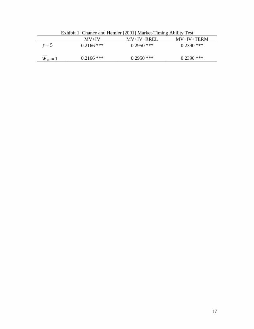
Chance and Hemler [2001] suggest that we can test market-timing abilities using

Spearman’s rank correlation between the weight of equities, ,M tW , and the excess stock

return, , 1 , 1m t f tR R+ +− . We consider the two specifications for γ ; however, as expected,

Exhibit 1 shows that the market-timing ability test does not depend on γ . Note that,

throughout the paper, ** and *** denote significance at the 5 percent and 1 percent

levels, respectively. We find that the correlation is positive and highly significant for all

three trading strategies, indicating that these forecasting variables have statistically

significant market-timing abilities.

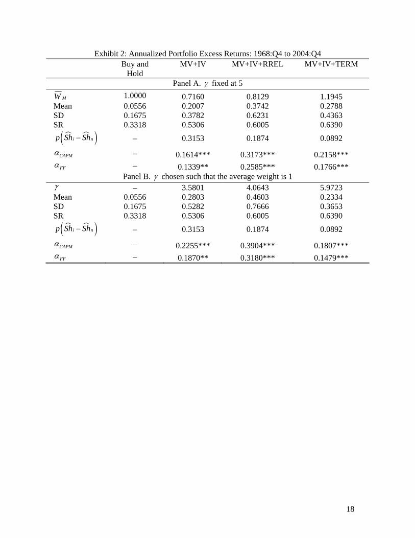
In Exhibit 2, we present summary statistics of annualized excess portfolio returns

for three timing strategies as well as the buy-and-hold strategy. Again, we consider two

specifications for γ : It is fixed at 5 in panel A and is chosen for each strategy such that

the average weight of equities is equal to 1 in panel B. We also report the average weight

of equities, MW , in panel A.

We first discuss the results in panel A of Exhibit 2. The trading strategy based on

MV and IV has an annualized average excess return of 20 percent, which is substantially

9

higher than 6 percent for the buy-and-hold strategy (row “Mean”). However, the former

has an annualized standard deviation of 38 percent, which is also much higher than 17

percent for the latter (row “SD”). Overall, the strategy based on MV and IV has an

annualized Sharpe ratio of 53 percent, compared with only 33 percent for the buy-and-

hold strategy (row “SR”). We also investigate whether the difference between the Sharpe

ratios is statistically significant using the Jobson and Korkie [1981] test with the Memmel

[2003] modification; in Table 2, “ ( )i np Sh Sh− ” denotes the associated significance

level. This test, however, needs to be interpreted with caution because, as noted by

Jobson and Korkie, it has low power in small samples. With this caveat in mind, we show

that the null hypothesis of no difference in the Sharpe ratios is not rejected at

conventional levels. However, we bootstrap excess returns on the S&P 500 and the

timing portfolio jointly and find less than a 14 percent chance of obtaining a Sharpe ratio

for the buy-and-hold strategy that is higher than the MV and IV strategy. Lastly, Jensen’s

alpha tests show that the excess portfolio return remains significantly positive after we

control for systematic risk using CAPM (row “ CAPMα ”) or the Fama and French 3-factor

model (row “ FFα ”). Also, we find that adding RREL (column “IV+MV+RREL”) or

TERM (column “IV+MV+TERM”) to the forecasting equation tends to improve the

Sharpe ratio. In particular, including TERM allows rejection of the same Sharpe ratio at

the 10 percent significance level. To summarize, market-timi3ng abilities of MV and IV

are both economically and statistically significant.

In panel B of Exhibit 2, we choose γ such that the average weight of equities for

each strategy is equal to 1 (row “γ ”). As expected, the main performance measures, e.g.,

the Sharpe ratio, the Jobson and Korkie [1981] test, and Jensen’s alpha tests, do not

10

change with γ . Note that the average returns differ somewhat from those reported in

panel A because of the different shares in equities. For brevity, we fix γ at 5 in the

remainder of the paper.

To investigate whether our results are driven by any particular event, we also

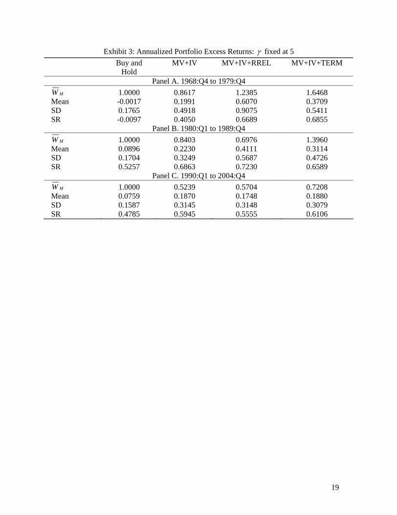
examine three subsamples: 1968:Q4-1979:Q4, 1980:Q1-1989:Q4, and 1990:Q1-2004:Q4.

As shown in Exhibit 3, all trading strategies produce higher excess returns and higher

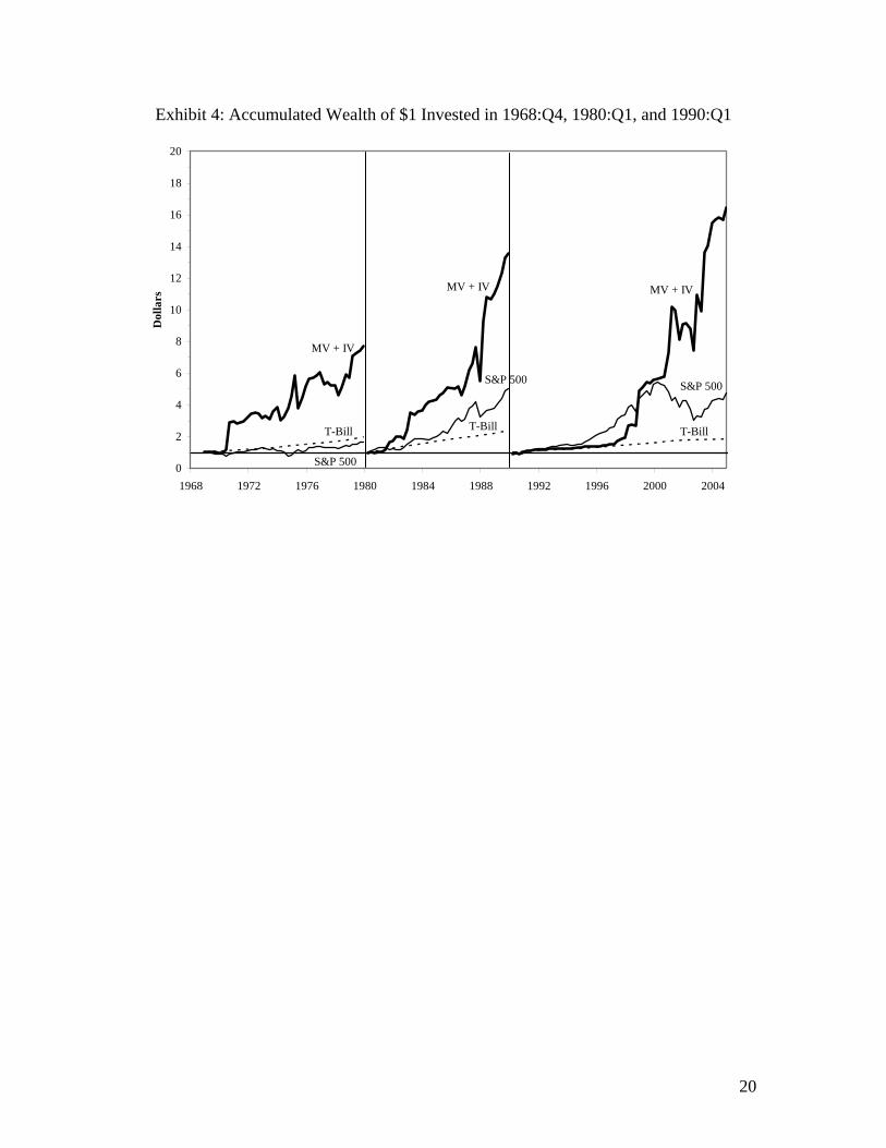
Sharpe ratios than the buy-and-hold strategy does in each of the subsamples. Exhibit 4

shows the accumulated wealth of one dollar invested during the three subsamples. The

accumulated wealth based on the MV and IV strategy is predominantly above that for the

strategy of investing only in the S&P 500 or 3-month T-bills. Therefore, in contrast with

early authors, e.g., Lee [1997], we find that the superior performance of the trading

strategy based on MV and IV is quite reliable across time.

Robustness Checks

We conduct a number of checks to ensure that our main results are robust. For

brevity, we provide only a brief summary here but details are available upon request. (1)

We conduct the market-timing ability test proposed by Cumby and Modest [1987] and

find essentially the same results. (2) We consider a switching strategy: Investors hold the

S&P 500 if the expected equity premium is positive and hold 3-month T-bills otherwise.

Although it is very conservative, the strategy based on MV and IV generates an

annualized average return and a Sharpe ratio of 6.4 percent and 47 percent, respectively,

which are noticeably higher than those for the buy-and-hold strategy (as reported in panel

11

A of Exhibit 2). (3) We estimate conditional stock market variance using the out-of-

sample forecast based on an autoregressive specification with two lags. In this case, the

managed portfolio based on MV and IV has an annualized average return and a Sharpe

ratio of 9.8 percent and 53 percent, respectively. (4) We consider a 25-basis-point

proportional (roundtrip) transaction cost, which is in the upper range for trading the S&P

500 (e.g., Balduzzi and Lynch [1999]). The transaction cost has a relatively small effect

on the results; for example, it reduces the strategy based on MV and IV by only 1.5

percent annually. (5) We use CRSP value-weighted stock market returns in place of the

S&P 500 returns and find essentially the same results. To summarize, our finding that

MV and IV have significant market-timing abilities appears to be quite robust.

Discussion and Conclusion

Many early authors, e.g., Samuelson [1994], have argued that stock market return

predictability cannot persist, once uncovered, for at least two reasons. First, in an

efficient market, investors will exploit the newly uncovered predictability until the

associated profit is arbitraged away. Second, stock return predictability might simply

reflect spurious data mining and thus cannot be used to form profitable trading strategies.

These explanations are plausible because, as mentioned above, stock return predictability

documented by early authors has indeed disappeared in the recent period.

Some recent authors (e.g., Campbell and Cochrane [1999] and Guo [2004]),

however, argue that stock return predictability reflects the time-varying risk premium and

thus cannot be arbitraged away. In particular, Merton’s ICAPM dictates a positive

relation between the conditional stock market risk and return. To exploit this relation, a

12

portfolio manager needs to buy stocks or provide liquidity to the stock market when

volatility rises—for example, as it did during the 1998 Russian default crisis—precisely

the time when investors want to bail out of the market.

To summarize, our analysis indicates that the trading strategy based on MV and

IV outperforms the buy-and-hold strategy, and the difference is very important

economically. The proposed strategy is easy to implement and quite reliable across time;

therefore, it might have important implications for portfolio management. However,

investors should be cautioned that the market-timing abilities of MV and IV might not

suggest an arbitrage opportunity because they could reflect time-varying systematic risk.

A further investigation of this issue is warranted and we leave it for future research.

13

Notes

1. Strictly speaking, the positive relation between the conditional excess stock market

return and variance holds only approximately because the conditional return is also

affected by the hedge demand for time-varying investment opportunities. See Merton

[1980] for conditions under which the effect of the hedge demand is negligible.

2. Alternatively and complementarily, Guo and Savickas [2005] also note that IV

forecasts stock returns possibly because it is a measure of variance of a priced risk factor,

which is omitted from standard asset pricing models (see, e.g., Lehmann [1990]).

14

References

Andrade, Sandro C., Ilona Babenko, and Yuri Tserlukevich. “Market Timing with Cay.”

Journal of Portfolio Management, forthcoming (2005).

Ang, Andrew, Robert Hodrick, Yuhang Xing, and Xiaoyan Zhang. "The Cross-Section of

Volatility and Expected Returns.” Journal of Finance, forthcoming (2005).

Balduzzi, Pierluigi, and Anthony Lynch. “Transaction Costs and Predictability: Some

Utility Cost Calculations.” Journal of Financial Economics, 52 (1999), pp. 47-78.

Boehme, Rodney, Bartley Danielsen and Sorin M. Sorescu. “Short Sale Constraints,

Differences of Opinion, and Overvaluation.” Journal of Financial and Quantitative

Analysis, forthcoming (2006).

Campbell, John, Y., and John Cochrane. “By Force of Habit: A Consumption-Based

Explanation of Aggregate Stock Market Behavior.” Journal of Political Economy, 107

(1999), pp. 205-251.

Campbell, John Y., Martin Lettau, Burton Malkiel and Yexiao Xu. “Have Individual

Stocks Become More Volatile? An Empirical Exploration of Idiosyncratic Risk.” Journal

of Finance, 56 (2001), pp. 1-43.

Chance, Don M., Michael Hemler. “The Performance of Professional Market Timers:

Daily Evidence from Executed Strategies” Journal of Financial Economics, 62 (2001),

pp. 377–411.

Cumby, Robert, and David Modest. “Testing for Market Timing Ability: A Framework

for Evaluation.” Journal of Financial Economics, 19 (1987), pp. 169-189.

Diether, Karl, Christopher J. Malloy, and Anna Scherbina. “Differences of Opinion and

the Cross Section of Stock Returns.” Journal of Finance, 57 (2002), pp. 2113-2141.

15

Fama, Eugene, and Kenneth French. “Common Risk Factors in the Returns on Stocks and

Bonds.” Journal of Financial Economics, 33 (1993), pp. 3-56.

French, Kenneth, William Schwert, and Robert Stambaugh. “Expected Stock Returns and

Volatility.” Journal of Financial Economics, 19 (1987), pp. 3-29.

Goyal, Amit, and Ivo Welch. “Predicting the Equity Premium with Dividend Ratios”

Management Science, 49 (2003), pp. 639-654.

Guo, Hui. "On the Real-Time Forecasting Ability of the Consumption-Wealth Ratio."

Working Paper 2003-007B, Federal Reserve Bank of St. Louis.

Guo, Hui. "Limited Stock Market Participation and Asset Prices in a Dynamic Economy"

Journal of Financial and Quantitative Analysis, 39 (2004), pp. 495-516

Guo, Hui, and Robert Savickas. “Idiosyncratic Volatility, Stock Market Volatility, and

Expected Stock Returns.” Journal of Business and Economics Statistics, forthcoming

(2005).

Guo, Hui. "On the Out-of-Sample Predictability of Stock Market Returns." Journal of

Business, forthcoming (2006).

Guo, Hui, and Robert Whitelaw. “Uncovering the Risk-Return Relation in the Stock

Market." Journal of Finance, forthcoming (2005).

Jobson, J. D., Bob Korkie. “Performance Hypothesis Testing with the Sharpe and

Treynor Measures” Journal of Finance, 36 (1981), pp. 889-908.

Lee, Wai. “Market Timing and Short-Term Interest Rates.” Journal of Portfolio

Management, 23 (1997) pp. 35-46.

Lehmann, Bruce. “Residual Risk Revisited.” Journal of Econometrics, 45 (1990), pp. 71-

97.

16

Lettau, Martin, and Sydney Ludvigson. “Consumption, Aggregate Wealth, and Expected

Stock Returns.” Journal of Finance, 56 (2001), pp. 815-849.

Merton, Robert. “An Intertemporal Capital Asset Pricing Model.” Econometrica, 41

(1973), pp. 867-887.

Merton, Robert. “On Estimating the Expected Return on the Market: An Exploratory

Investigation.” Journal of Financial Economics, 8 (1980), pp. 323-361.

Memmel, Christoph. “Performance Hypothesis Testing with the Sharpe Ratio.” Finance

Letters, 1 (2003), pp. 21-23.

Miller, Edward. “Risk, Uncertainty, and Divergence of Opinion.” Journal of Finance, 32

(1977), pp. 1151-1168.

Shalen, Catherine T. “Volume, Volatility, and the Dispersion of Beliefs.” Review of

Financial Studies, 6 (1993), pp. 405-434.

Shen, Pu. “Market Timing Strategies That Worked: Based on the E/P Ratio of the S&P

500 and Interest Rates.” Journal of Portfolio Management, 29 (2003) pp. 57-68.

Samuelson, Paul A. “The Long-Run Case for Equities.” Journal of Portfolio

Management, 21 (1994), pp. 15-24.

17

Exhibit 1: Chance and Hemler [2001] Market-Timing Ability Test MV+IV MV+IV+RREL MV+IV+TERM

5γ = 0.2166 *** 0.2950 *** 0.2390 ***

1MW = 0.2166 *** 0.2950 *** 0.2390 ***

18

Exhibit 2: Annualized Portfolio Excess Returns: 1968:Q4 to 2004:Q4 Buy and

Hold MV+IV MV+IV+RREL MV+IV+TERM

Panel A. γ fixed at 5

MW 1.0000 0.7160 0.8129 1.1945 Mean 0.0556 0.2007 0.3742 0.2788 SD 0.1675 0.3782 0.6231 0.4363 SR 0.3318 0.5306 0.6005 0.6390

( )i np Sh Sh− – 0.3153 0.1874 0.0892

CAPMα – 0.1614*** 0.3173*** 0.2158*** FFα – 0.1339** 0.2585*** 0.1766***

Panel B. γ chosen such that the average weight is 1 γ – 3.5801 4.0643 5.9723 Mean 0.0556 0.2803 0.4603 0.2334 SD 0.1675 0.5282 0.7666 0.3653 SR 0.3318 0.5306 0.6005 0.6390

( )i np Sh Sh− – 0.3153 0.1874 0.0892

CAPMα – 0.2255*** 0.3904*** 0.1807*** FFα – 0.1870** 0.3180*** 0.1479***

19

Exhibit 3: Annualized Portfolio Excess Returns: γ fixed at 5 Buy and

Hold MV+IV MV+IV+RREL MV+IV+TERM

Panel A. 1968:Q4 to 1979:Q4 MW 1.0000 0.8617 1.2385 1.6468

Mean -0.0017 0.1991 0.6070 0.3709 SD 0.1765 0.4918 0.9075 0.5411 SR -0.0097 0.4050 0.6689 0.6855

Panel B. 1980:Q1 to 1989:Q4 MW 1.0000 0.8403 0.6976 1.3960

Mean 0.0896 0.2230 0.4111 0.3114 SD 0.1704 0.3249 0.5687 0.4726 SR 0.5257 0.6863 0.7230 0.6589

Panel C. 1990:Q1 to 2004:Q4 MW 1.0000 0.5239 0.5704 0.7208

Mean 0.0759 0.1870 0.1748 0.1880 SD 0.1587 0.3145 0.3148 0.3079 SR 0.4785 0.5945 0.5555 0.6106

20

Exhibit 4: Accumulated Wealth of $1 Invested in 1968:Q4, 1980:Q1, and 1990:Q1

0

2

4

6

8

10

12

14

16

18

20

1968 1972 1976 1980 1984 1988 1992 1996 2000 2004

Dol

lars

MV + IV

MV + IV MV + IV

T-Bill T-Bill T-Bill

S&P 500

S&P 500 S&P 500