Marketmaking Middlemen∗

Pieter Gautier † Bo Hu‡ Makoto Watanabe§

† ‡ § VU University Amsterdam, Tinbergen Institute

April 7, 2015

Very Preliminary

Abstract

This paper develops a model in which market structure is determined endogenously

by the choice of intermediation mode. We consider two representative business modes

of intermediation that are widely used in real-life markets: one is a market-making

mode by which an intermediary offers a platform for buyers and sellers to trade by

their own; the other is a middleman mode by which an intermediary holds inventories

which he stocks from sellers for the purpose of reselling to buyers. In our model,

buyers and sellers have an option of searching in an outside market as well as using the

service offered by a monopolistic intermediary. We derive the conditions under which

the mixture of the two intermediation modes is selected over an exclusive use of either

of the modes.

Keywords: Middlemen, Marketmakers, Platform, Search

JEL Classification Number:D4, F1, G2, L1, L8, R1

∗We thank seminar and conference participants at U Essex, U Bern, U Zurich, and the Symposium on JeanTirole 2014 for useful comments.†VU University Amsterdam, Tinbergen Institute, Address: Department of Economics, VU Amsterdam, De

Boelelaan 1105, NL-1081 HV Amsterdam, The Netherlands, p.a.gautier@vu.nl‡VU University Amsterdam, Tinbergen Institute, Address: Department of Economics, VU Amsterdam, De

Boelelaan 1105, NL-1081 HV Amsterdam, The Netherlands, huboshufe@gmail.com§VU University Amsterdam, Tinbergen Institute, Address: Department of Economics, VU Amsterdam, De

Boelelaan 1105, NL-1081 HV Amsterdam, The Netherlands, makoto.wtnb@gmail.com

1

1 Introduction

This paper considers a framework in which market structure is determined by the intermediation

service offered to customers. We consider two representative business modes of intermediation

that are widely used in real-life markets. In one mode, an intermediary acts as a middleman (or

a merchant), who is specialized in buying and selling by his own account and typically operates

by holding inventory (e.g. supermarkets, and traditional brick and mortar retailers). In the other

mode, an intermediary acts as a marketmaker, who offers a marketplace or a platform where the

participating buyers and sellers trade with each other (e.g. eBay).

In most real-life markets, however, intermediaries are not one of those extremes but operate

both as a middleman and a marketmaker at the same time. This is what we call a marketmaking

middleman.1 For example, the well-known electronic intermediary Amazon, one of the largest

marketmaking middlemen nowadays, started off as a pure middleman, buying and reselling prod-

ucts in its own name since its founding in 1994. In the early 2000s, Amazon moved toward a

marketmaker, by allowing other suppliers to participate as independent sellers. In 2014, those

independent sellers accounted for 50% of gross merchandise volume of Amazon. Similar operation

patterns are used by both Rakuten and JD.com, which are Amazon’s counterparts in Japan and

China. Other examples of marketmaking middlemen include real-estate agents, dealer/brokers in

financial markets, and department stores.2

We present a model in which the intermediated-market structure is determined endogenously

as a result of the strategic choice of a monopolistic intermediary. In our model, there are two

markets open to individuals, one is an intermediated market operated by the intermediary, and

the other is a decentralized market where buyers and sellers search randomly. The intermediated

market combines two business modes: acting as a middleman, the intermediary is prepared to

serve many buyers at a time by holding inventories; acting as a marketmaker, the intermediary

offers a platform. The intermediary’s decision is essentially about how to allocate the attending

buyers among these two business modes.

1In the finance literature, different terminologies are used to classify the type of intermediaries: brokers refer tointermediaries who do not trade for their own account, but act merely as conduits for customer orders, akin to ourmarketmakers; dealers refer to intermediaries who do trade for their own account, akin to our middlemen/merchants.The marketmakers (or specialists) in financial markets correspond broadly to our market-making middlemen, sincethey quote prices to buy or sell the asset as well as take market positions.

2In particular, real-estate agents match buyers and sellers, and also stock properties themselves for sale;dealer/brokers in financial markets engage in trading securities on behalf of clients as well as for their own ac-counts; some department stores also rent shelf spaces to manufacturers. Further examples can be found in Hagiuand Wright (2015).

2

In either way of intermediated trade, we formulate the intermediated market as a directed

search market in order to feature the intermediary’s technology of spreading price and capacity

information efficiently.3 In addition, this approach enables us to highlight the middleman’s ad-

vantage in the high selling capacity that mitigates search frictions and provides customers with

proximity. Thus, the middleman mode outperforms the marketmaker mode in allocation effi-

ciency. The decentralized market represents an individuals’ outside option that determines the

lower bound of their market utility.

With this set up, we consider two situations, single-market search versus multiple-market

search. With the single market search, agents have to choose which market to search in advance,

either the decentralized market or the intermediated market. This implies that the intermediary

needs to subsidize either buyers or sellers with their expected value in the decentralized market,

but once they participate, the intermediated market operates without fear of competitive pressure

outside. In this situation, the intermediary can extract the individual surplus monopolistically for

each realized transaction. This can be done either by setting a monopolistic intermediation fee as

a marketmaker, or by charging a monopolistic price for the inventory as a middleman – in either

way, the per-transaction profits are the same. Given the middleman mode is more efficient in

realizing transactions, the intermediary uses the middleman-mode exclusively when agents search

a single market.

When agents are allowed to search multiple markets, attracting buyers and sellers becomes less

costly compared to the single-market search case — the intermediary does not need to subsidy

either of the sides to induce participation. However, this time, the prices/fees charged in the

intermediated market must be acceptable relative to the available option in the decentralized

market. Thus, with the multiple-market search, the outside option creates competitive pressure

to the overall intermediated market. On the one hand, a higher capacity of the middleman leads

to a larger number of successful transactions in the intermediated market. This happens due to

the demand stimulating effect: a higher capacity induces more buyers to buy from the middleman,

and fewer buyers to search in the platform, which increases the intermediary’s profit. On the other

hand, the demand effect makes sellers less likely to be successful in the platform, so that more

sellers are available when a buyer attempts to search in the decentralized market. Accordingly, the

buyers expect a higher value from the decentralized market, which causes a competitive pressure on

3Using the search function in the Amazon website, for example, one can receive instantly all relevant informationsuch as prices, stocks of individual sellers and Amazon’s inventories.

3

the price that the intermediary can charge. Hence, the intermediary trade-offs a larger quantity

against lower price/fees to operate as a larger-scaled middleman. This trade-off pins down an

optimal structure of intermediation modes.

In real-life economy, the single-market search may correspond to the traditional search tech-

nology for supermarkets or brick and mortar retailers. Over the course of shopping trip under

such a market structure, consumers usually have to search, buy and transport the purchased items

during a fixed amount of time. Given the time constraint, they visit a limited number of shops –

typically one supermarket –, and appreciate the proximity provided by its inventory. In contrast,

the multi-market search may be related to the advanced search technologies available in the digital

economy. Such a technology may allow the online-customers to search with ease and convenience,

and to compare various options. A similar can happen in the market for durable goods such as

housing or expensive items where customers are usually exposed for a sufficiently long time period

to ponder multiple available options thoroughly.

Given these technologies, our theory is in line with a casual observation that internet inter-

mediaries such as Amazon and e-Bay often face massive offline competitors, and by organizing

a platform, they attract offline sellers. Eventually, the burgeon of the online/mobile commerce

sometimes leads to the decline of high street retailers.

The comparison of the above two cases delivers an interesting policy implication of intermedi-

ated markets. In our economy, the optimal business mode from the social planner’s viewpoint is

the middleman mode because it minimizes market frictions and can implement an efficient trade.

In the presence of outside competition, however, using a platform can be profitable for the inter-

mediary and it reduces its inventory from the efficient level. Hence, competition for intermediation

can deteriorate efficiency and welfare.

This paper contributes to two strands of literature. One is the literature of middlemen de-

veloped by Rubinstein and Wolinsky (1987), Duffie, Garleanu, and Pedersen (2006), Lagos and

Rocheteau (2009), Shevichenko (2004), Johri and Leach (2002), Masters (2007), and Wong and

Wright (2014).4 Using a directed search approach, Watanabe (2010, 2013) provide a model of an

intermediated market operated by middlemen with high inventory holdings. The middlemen’s high

4Rubinstein and Wolinsky (1987) show that an intermediated market can be active under frictions, when itis operated by middlemen who have an advantage in the meeting rate over the original suppliers. Given someexogenous meeting process, two main reasons have been considered for the middlemens advantage in the rate ofsuccessful trades: a middleman may be able to guarantee the quality of goods (Biglaiser, 1993, Li, 1998), or tosatisfy buyers demand for a varieties of goods (Shevichenko, 2004). While these are clearly sound reasons forthe success of middlemen, the buyers search is modeled as an undirected random matching process, thereby themiddlemens capacity cannot influence buyers search decisions in these models.

4

capacity enables them to serve many buyers at a time, thus to lower the likelihood of stock-out,

which generates a retail premium of inventories. This mechanism is adopted by the middleman

in our model as well. Hence, if there is no market-making mode, then our model is a simplified

version of Watanabe where we added an outside market. It is worth mentioning that in Watanabe

(2010, 2013), the middleman’s inventory is modeled as a discrete unit, i.e., a positive integer, so

that the middlemen face a non-degenerate distribution of their selling units as other sellers do.

In contrast, we model the inventory as measured by mass, assuming more flexible inventory tech-

nologies, so that the middleman faces a degenerate distribution of sales. This simplification allows

us to characterize the middleman’s profit maximizing level of inventory – in Watanabe (2010)

the inventory level of middlemen is determined by aggregate demand-supply balancing. Recently,

Holzner and Watanabe (2015) study a labor market equilibrium using a directed search approach

to model a job-brokering service (i.e., a market-making service), offered by Public Employment

Agencies, but the choice of intermediation mode is not the scope of their paper.

The other related strand is the two-sided market literature, e.g. Rochet and Tirole (2003,

2006), Caillaud and Jullien (2003), Rysman (2004), Armstrong (2006), Hagiu (2006) and Weyl

(2010).5 The critical feature of platform is the presence of the cross-group externality, i.e. the

participants’ expected gains from a platform depend positively on the number of participants on

the other side of it. When such a cross-group externality exists, the marketmaker can use “divide-

and-conquer” strategies, namely, subsidizing one group of participants in order to attract another

group and extract the ensuing externality benefit (see, Caillaud and Jullien, 2003). This strategy

is adopted by the intermediary in our model as well. Broadly speaking, if there is no middleman

mode, then our model is a directed search version of Caillaud and Jullien (2003) in combination

with a decentralized market.

Finally, Hagiu and Wright (2015) study the profitability of intermediation modes as is de-

termined by marketing activities. In their model, it is assumed that the owner of a product has

private information on how effective their marketing activity will be. Then, they show that the op-

timal design of intermediation mode is determined, among others, by the cross-product spillovers

of marketing activity, and the degree of owners’ informational advantage. For each product, an

intermediary only takes the preferred extreme mode instead of a hybrid one, and their theory

5Closely related papers based on a similar spirit can be found in Baye and Morgan (2001), Rust and Hall (2003),Nocke et al. (2007), Loertscher (2007), Galeotti and Moraga-Gonzalez (2009) and Edelman and Wright (2015). Forearlier contributions of this strand of literature, see, e.g., Stahl (1988), Gehrig (1993), Yavas (1994, 1996), Spulber(1996) and Fingleton (1997).

5

explains which products the intermediary should offer in which mode. In contrast, we show that

even for a homogeneous product and homogeneous agents, a hybrid intermediation mode can oc-

cur in equilibrium. As the driving force of our result is the competitive thread, our theory explains

how the intermediary should organize its intermediated structure depending on the competitive

environment.

The rest of the paper is organized as follows. Section 2 presents the basic setup and section

3 studies the optimal strategy of a marketmaker mode. Section 4 brings the middleman mode

into the benchmark model and characterizes the intermediary’s optimal strategy under exclusivity.

Section 5 extends the analysis to allow for non-exclusivity and gives the key finding of the paper.

Section 6 discusses the welfare and other modeling issues. Section 7 concludes. Some proofs are

in the appendix.

2 Setup

We consider a large economy with two types of agents: a mass B of buyers and a mass S of

sellers. Agents of each type are homogeneous. Each buyer has unit demand of a homogeneous

good, and each seller has a production technology of that good. The consumption value for the

buyer is normalized to 1. The marginal production cost is denoted by c ∈ [0, 1). Sellers are able

to produce as much as they want but their selling/trading capability is limited so that each seller

can sell only one unit of the good.

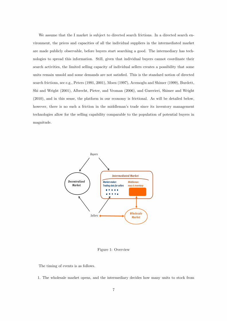
There are two retail markets, an intermediated market and a decentralized market (see Figure

1). The decentralized market (hereafter D market) is featured by random matching and bilateral

bargaining. Without loss of generality, we assume that a buyer finds a seller with probability λb

and a seller finds a buyer with probability λs, satisfying Bλb = Sλs and λb, λs ∈ (0, 1). This linear

matching technology is extended to general non-linear matching functions in Section 6. Matched

partners follow an efficient bargaining process, which yields a linear sharing of the total surplus,

with β ∈ (0, 1) as the share for the buyer, and 1− β for the seller.

The intermediated market (hereafter I market) is operated by a monopolistic intermediary. The

intermediary can perform two different intermediation activities. As a middleman, he purchases

a good from sellers in a competitive wholesale market, and holds it as an inventory to resell to

buyers. As a marketmaker, he does not buy and sell but instead provides a platform where buyers

and sellers can trade with each other upon paying transaction fees and registration fees.

6

We assume that the I market is subject to directed search frictions. In a directed search en-

vironment, the prices and capacities of all the individual suppliers in the intermediated market

are made publicly observable, before buyers start searching a good. The intermediary has tech-

nologies to spread this information. Still, given that individual buyers cannot coordinate their

search activities, the limited selling capacity of individual sellers creates a possibility that some

units remain unsold and some demands are not satisfied. This is the standard notion of directed

search frictions, see e.g., Peters (1991, 2001), Moen (1997), Acemoglu and Shimer (1999), Burdett,

Shi and Wright (2001), Albrecht, Pieter, and Vroman (2006), and Guerrieri, Shimer and Wright

(2010), and in this sense, the platform in our economy is frictional. As will be detailed below,

however, there is no such a friction in the middleman’s trade since its inventory management

technologies allow for the selling capability comparable to the population of potential buyers in

magnitude.

Pure marketmakerPure middleman Marketmaking middleman

DecentralizedMarket

Sellers

Buyers

WholesaleMarket

SupermarketsRetailersiTunes

eBay, TaobaoApple storeGoogle Play

Amazon, bol.com, RakutenReal estate agentsDealers in financial markets

Market-maker:Trading slots for sellers

Middleman:mass k inventory

Intermediated Market

Figure 1: Overview

The timing of events is as follows.

1. The wholesale market opens, and the intermediary decides how many units to stock from

7

sellers. The amount of inventory is denoted by k ∈ [0, B]. There is no limit on sellers’

production capacity, hence the inventory demand of the middleman can always be satisfied.

We assume the wholesale market to be competitive so that the wholesale price equals the

marginal production cost c. The wholesale market then closes.

2. Two retail markets open to buyers and sellers, an I market and a D market. The I market is

operated by the intermediary, who announces its inventory k for the middleman sector, and

a set of fees F ≡{f b, fs, gb, gs

}for participation and transaction in the marketmaker sector.

In particular, f b, fs ∈ [0, 1] is a transaction fee charged to a buyer or a seller, respectively,

and satisfies f ≡ f b + fs ∈ [0, 1], gb, gs ∈ [−1, 1] is a registration fee charged to a buyer or

a seller, respectively.

3. Observing the fees F and inventory k, buyers and sellers simultaneously decide which market

to participate in. In Section 3 and 4, we explore the exclusivity case where they can only

attend one market. In Section 5, we consider the non-exclusivity case where they can attend

both markets sequentially.

4. Once in the I market, buyers and sellers as well as the middleman are engaged in a standard

directed search game that determines the equilibrium price for individual sellers ps and the

middleman pm, as will be detailed shortly below.

3 Directed search model of marketmaker

Assuming for the moment k = 0, we start with the case where the middlemen option is absent

so the only intermediation is a marketmaker mode. We also restrict the meeting technology

to be exclusive so that agents are allowed to visit only one market, either the C or D market.

Our derivation follows backward induction. We starts with an analysis of the directed search

equilibrium in the C market, and then solve for the intermediary’s optimal fees F .

Directed search equilibrium in the marketplace Given an announced set of fees, suppose

that a mass BC of buyers and a mass SC of sellers have decided to participate in the C market.

Then, the C market has the following stages. In the first stage, all the participating sellers

simultaneously post a price which they are willing to sell at. Observing the prices, all buyers

simultaneously decide which seller to visit in the second stage. Each buyer can visit one seller. If

8

more than one buyer visits a seller, then the good is allocated randomly. Assuming buyers cannot

coordinate their actions over which seller to visit, a symmetric equilibrium is investigated where

all buyers use an identical visiting strategy for any configuration of the announced prices, and all

sellers play the same strategy which in this case implies that they post an identical price denoted

by ps.

Each individual seller is characterized by an expected queue of buyers, denoted by x. The

number of buyers visiting a given seller who has expected queue x is a random variable, denoted

by N , which in a larger market has a Poisson distribution, Prob[N = n] = e−xxn

n! . In a symmetric

equilibrium where xs is the expected queue length of buyers at a seller, each buyer visits some

seller with probability SCxs. They should satisfy the accounting identity,

SCxs = BC , (1)

requiring that the number of buyers visiting individual sellers sums up to the total population of

buyers. The buyer’s probability of being served by a seller depends on the expected queue length

xs and is denoted by ηs(xs). The equilibrium values of buyers and sellers, denoted by V b and V s

respectively, should satisfy

V b = ηs (xs) (1− ps − f b)

V s = xsηs (xs) (ps − fs − c).

Given a symmetric equilibrium, suppose a seller deviates to a price pd 6= ps. If a buyer visits

this deviating seller then the probability that it will get served is given by

ηs(xd)

=1− e−xd

xd,

where xd is the expected queue length for this deviating seller. To understand this probability,

note that the probability of this seller to receive at least one buyer is given by xdηs(xd) = 1−e−xd

where e−xd

= Prob[N = 0]. Since buyers must be indifferent between visiting any sellers (including

the deviating seller), the buyer’s market utility condition is

V b = ηs(xd)

(1− pd − f b).

Given V b, this equation determines the relationship between xd and pd, which we denote by

xd = xd(pd|V b). Since in a large market, individual buyers and sellers cannot affect market

utility, the deviant takes V b as given and V b does not depend on pd.

9

We now determine the equilibrium price. Taking into account the relationship between the

expected queue length xd and price pd, the optimal price pd∗ has to maximize the expected payoff

of the deviant,

pd∗ = argmaxpdxd(pd)ηs

(xd(pd)

)(pd − fs − c).

Since there exists a one to one relationship between pd and xd, the problem can be written as

if the seller selects a queue length xd rather than a price pd. Hence, substituting out the price

pd = 1− f b − xd

1−e−xdV b, the expected profit of the seller with queue length xd is

(1− e−x

d)

(1− f − c)− xdV b,

where f ≡ fs + f b is the sum of transaction fees. Taking V b as given, the first order condition

with respect to xd yields V b = e−xd∗

(1 − f − c). In a symmetric equilibrium, the optimal xd∗

coincides with the equilibrium expected queue length, xd∗ = xs. Hence,

V b = e−xs

(1− f − c). (2)

The second order condition is satisfied. Substituting it back into the price, the equilibrium price

can be written as

ps = 1− f b − xse−xs

1− e−xs(1− f − c). (3)

Finally, the value for a seller is

V s =(

1− e−xs

− xse−xs)

(1− f − c). (4)

Lemma 1 Given an announced set of fees, F = {f b, fs, gb, gs}, suppose that BC > 0 buyers

and SC > 0 sellers have decided to participate in the C market. Given that the intermediary

has no inventory k = 0 and acts as a marketmaker, a directed search equilibrium in marketplace

exists and is unique. It is described as a queue of buyers, xs ∈ (0, BC/SC), an equilibrium price

ps ∈ (0, 1), the value of buyers V b ∈ (0, 1) and the value of sellers V s ∈ (0, 1), satisfying (1), (3),

(2) and (4), respectively.

Define the matching elasticity as βC ≡dxsηs(xs)/dxs

xsηs(xs)/xs = xse−xs

1−e−xs ∈ (0, 1). In the directed search

equilibrium, sellers are matched with probability xsηs(xs) = 1 − e−xs

, and get a revenue of

ps − fs − c = (1− βC)(1− f − c) and buyers are matched with probability ηs(xs) = 1−e−xs

xs and

gain 1 − f b − ps = βC(1 − f − c). Hence, it is clear that whoever bears the transaction fee does

10

not matter because the equilibrium price will adjust so that the total surplus 1− f − c is always

divided according to the share βC . Hereafter, we assume that buyers pay all the transaction fees.

Marketmaker’s problem To model how the intermediary should set fees, we follow the lit-

erature of two-sided markets (Caillaud and Jullien, 2003). In particular, we assume that agents

hold pessimistic expectations on the participation decision of agents on the other side of the mar-

ket. More precisely, in a bad-expectation market allocation, users coordinate on a distribution

that yields minimal profits for the marketmaker. For instance, a pessimistic expectation of sellers

means that sellers believe the number of buyers registering with the C market is zero whenever

λbβ (1− c) > −gb,

where λbβ (1− c) is the expected payoff of buyers in the D market and they believe that no sellers

would be in the C market so that all buyers receive in the C market is −gb (it is a participation

subsidy when gb < 0).

Under those beliefs, a profitable strategy for the marketmaker is necessarily a divide-and-

conquer strategy. To divide buyers and conquer sellers, referred to as a DbCs strategy, it is

required that

Db : −gb ≥ λbβ (1− c) , (5)

Cs : V s − gs ≥ 0. (6)

The divide-condition Db tells us that the marketmaker should provide a negative entrance fee to

buyers so that the participating buyers can be guaranteed at least what they would get in the D

market, even if no sellers were operating in the C market. This makes sure that buyers will join

the marketplace. The conquer-condition Cs guarantees the participation of sellers, by giving them

a nonnegative payoff. Since under this strategy all buyers are in the C market, and the D market

is empty, the expected payoff from the D market is zero. Here, the expected value of sellers in the

C market V s is as given by (4), and all the agents will participate in the C market, i.e., BC = B

and SC = S.

Similarly, a strategy to divide sellers and conquer buyers (DsCb) requires that

Ds : −gs ≥ λs(1− β) (1− c) , (7)

Cb : V b − gb ≥ 0. (8)

11

Under either of the divide-and-conquer strategies, the marketmaker’s expected profit is

Π = Bgb + Sgs + Tf,

where Bgb and Sgs are registration fees from buyers and sellers, Tf is the transaction fee, T ≡

S(1−e−xs) is the expected amount of trades in the marketplace. Substituting the binding divide-

and-conquer constraints, the expected profits with a DbCs strategy or a DsCb strategy, denoted

by ΠDbCs and ΠDsCb respectively, are given by

ΠDbCs = −Bλbβ (1− c) + S(

1− e−xs)

(ps + f − c) , (9)

ΠDsCb = −Sλs(1− β) (1− c) + S(

1− e−xs)

(1− ps) , (10)

where the expected queue length of buyers is xs = BS .

Substituting equilibrium price (3) and taking derivatives with respect to f , we have

∂ΠDbCs

∂f= Sxse−x

s

> 0,

∂ΠDsCb

∂f= S(1− e−x

s

− xse−xs

) > 0.

Thus, the optimal transaction fee is given by f = 1− c, and

ΠDbCs =[−Bλbβ + S(1− e−x

s

)]

(1− c) ,

ΠDsCb =[−Sλs(1− β) + S(1− e−x

s

)]

(1− c) .

The intuition is as follows. An increase in f merely implies transfers from buyers and sellers

to the intermediary. A higher f certainly harms buyers and sellers, and the registration fees

decline correspondingly. The result of the trade-off is determined by the fact that using a divide

and conquer strategy only the value of one type of agents can be collected using registration

fees. Therefore, in the perspective of the intermediary, the overall effect of f is positive. The

intermediary would like to set f as high as possible. To summarize the analysis so far, we get the

following proposition.

Proposition 1 Given k = 0, the profit-maximizing transaction fee set by a monopolistic market-

maker is f = 1−c. When β < 1−β, the marketmaker divides buyers and conquers sellers (DbCs)

by setting gb = −λbβ (1− c) and gs = 0. When β > 1 − β, the marketmaker divides sellers and

conquers buyers (DsCb) by setting gs = −λs(1− β) (1− c) and gb = 0.

12

The profit-maximizing marketmaker subsidies one side by guaranteeing their outside value,

and then profits from the other side by charging them the highest possible transaction fee. Since

Bλb = Sλs, it is the value of bargaining power β that decides which side should be subsidized

(divided). When β < 1 − β, it is less costly to divide buyers and conquer sellers, whereas when

β > 1− β, it is less costly to divide sellers and conquer buyers.

4 Single-market search

In this section, we introduce the middleman mode, that is k ≥ 0, into the directed search framework

set out in the last section and explore the optimal structure of a hybrid intermediary under

exclusive service.

4.1 Directed search equilibrium in the marketplace

If the intermediary also works as a middleman by holding its own inventory, then in the centralized

market there are three types of agents: a mass BC of buyers, a mass SC of sellers and the in-

termediary/middleman. The symmetric equilibrium is characterized by an expected queue length

xs per seller, and an expected queue length xm of the middleman. They satisfy the accounting

identity,

SCxs + xm = BC , (11)

requiring that the number of buyers visiting individual sellers and the middleman sums up to the

total population of buyers.

Since the middleman has a continuum inventory, total matched buyers at the middleman equals

the minimum of inventory and the mass of visiting buyers, min {k, xm}. The probability for a

buyer to be served at the middleman is

ηm (xm) =min {k, xm}

xm.

Given this probability, the equilibrium values of buyers at sellers and the middleman in the C

market, denoted by V b(s) and V b(m) respectively, are given by

V b(s) = ηs(xs) (1− ps − f) ,

V b(m) = ηm (xm) (1− pm) ,

where ηs(xs) ≡ 1−e−xs

xs as defined before. In equilibrium, buyers should be indifferent between

visiting sellers and the middleman, thus V b(s) = V b(m).

13

Next, turn to the supply side. The value of an independent seller is

V s = xsηs(xs) (ps − c) .

The value of the intermediary consists of two parts, the profit of the middleman sector

xmηm (xm) pm − kc, and the profit from organizing the marketplace BCgb + SCgs + Tf, where

T ≡ SC(1− e−xs

)equals the expected platform transactions. Under pessimistic expectations, the

intermediary must employ divide-and-conquer strategies to attract users. Using these strategies

all the agents will participate in the C market, i.e., BC = B and SC = S. Taking inventory k and

the set of fees F as given, the intermediary’s expected profit is

Π (pm; k, F ) = Bgb + Sgs + Tf + xmηm (xm) pm − kc.

Notice at the moment that sellers and the middleman post prices, registration fees gb, gs are paid

and thus are taken as given.

Let’s turn to the determination of ps. ps can be derived by considering a deviating seller setting

pd 6= ps. This part is similar as in section 3. The expected queue length for this deviating seller

is denoted by xd. In the equilibrium, buyers must be indifferent between visiting this deviating

seller and other sellers,

V b = ηs(xd)(1− pd − f

).

Each seller is infinitely small, and can’t influence the market utility of buyers, thus from the

deviant’s perspective, V b can be treated as a constant. To determine the optimal price pd∗,

substitute the price pd = 1− f − xd

1−e−xdV b into V s

V s(xd)

=(

1− e−xd)

(1− f − c)− xdV b.

The first order condition with respect to xd is e−xd∗

(1− f − c) − V b = 0. In a symmetric

equilibrium, the optimal arrival rate xd∗ is equal to the equilibrium arrival rate, i.e. xd∗ = xs.

This leads to

V b(s) = e−xs

(1− f − c) (12)

The second order condition is satisfied. Substituting it back yields the optimal retail price of

sellers

ps = 1− f − xse−xs

1− e−xs(1− f − c) , (13)

14

and the equilibrium value of sellers

V s =(

1− e−xs

− xse−xs)

(1− f − c) . (14)

We now turn to pm. First, it is easy to see that xm can’t be larger than B as there are simply

no more than B buyers. Also, any k > B will not help to improve the matching probability,

but only incur extra inventory costs. Without loss of generality, we impose xm, k ∈ [0, B]. The

optimal retail price pm is characterized by maximizing the intermediary’s expected profit taking k

and f as given, subject to the condition that buyers are indifferent between visiting independent

sellers and the middleman,

V b = ηm (xm) (1− pm) .

Critically, the intermediary holds a continuum of inventories so that it can influence V b and

xs purposely. To reflect all these effects, we should take into account that xs (xm) and V b (xm)

are functions of xm satisfying (11) and (12). Thus, the buyers’ indifference condition V b(s) = V b(m)

becomes

pm (xm) = 1− 1

ηm (xm)e−

B−xmS (1− f − c) . (15)

This expression clearly states that pm is positively correlated with the transaction fee f . In

particular, when f is not bounded above, that is f = 1 − c is feasible, the intermediary sets

a monopoly price for its inventory pm = 1, which makes the middleman mode more profitable;

when f is bounded above due to outside competition, the monopoly price is not possible, and the

marketmaking mode might become more attractive. Whether f will be restricted depends on the

market structure and the configuration on exclusivity. As we shall see later, the restriction on f

is the key factor for the intermediary’s optimal structure.

Substituting pm from (15), the problem can be regarded as if the intermediary is choosing an

expected queue xm instead of the price,

maxxm

Π (xm; k, F ) = Bgb + Sgs + Tf + xmηm (xm) pm (xm)− kc. (16)

This problem can be easily solved as shown in Lemma 2.

Lemma 2 Given B > 0, S > 0, f ∈ [0, 1− c] and k ∈ [0, B], the optimal expected queue length of

the middleman satisfies xm = min {x̃m (f) , k} , where x̃m (f) ∈ (0, B] satisfies

1− e−B−xmS − xm

Se−

B−xmS (1− f − c) = 0.

15

The intuition behind the lemma is as follows. Given the coordination frictions in the inter-

mediated platform, a larger middleman sector creates more transactions that potentially gives

higher profits. However, to attract more buyers to the middleman (a higher xm), the interme-

diary has to lower the price pm and give buyers a higher surplus V b. This trade off determines

the unique x̃m (f). Moreover, having more buyers than the inventory xm > k does not increase

transactions since it is bounded above by k. This suggests any xm > k can’t be optimal. That is,

xm = min {x̃m (f) , k}.

As shown in the lemma, inventory k only plays a role as a turning point of the piecewise

profit function, and thus any interior solution of xm is not affected by the value of k. This

feature will help to further clarify the optimal k in the first stage of the game. We thus finish the

characterization of the directed search equilibrium, which is summarized in the following lemma.

Lemma 3 Given an announced set of fees, F = {f, gb, gs}, inventory k, a mass of B > 0

buyers and a mass of S > 0 sellers have decided to participate in the C market, a directed search

equilibrium in the marketplace exists and is unique. It is described by queues of buyers at each

seller, xs ∈ (0, B/S), and at the middleman, xm ∈ (0, B), equilibrium prices ps, pm ∈ (0, 1), and

the value of buyers V b ∈ (0, 1), of sellers V s ∈ (0, 1), and of the intermediary Π ∈ (0, B) satisfying

(11), (12), (13), (15), (14), (16) and lemma 2.

4.2 Intermediation structure and fees

At the first stage of the game, the intermediary chooses inventory k and the fee structure F ,

taking into account of its effect on xm (k, F ). The divide and conquer conditions (5), (6), (7) and

(8) of section 3 continue to hold. Substituting them into (16) leads to profits for each strategy.

The DbCs strategy divides buyers by gb = −λbβ (1− c) and extracts gs = V s from sellers by

registration fees,

ΠDbCs = −Bλbβ (1− c) + S(

1− e−xs)

(ps + f − c)

+xmηm (xm) pm − kc. (17)

The DsCb strategy divides sellers by gs = −λs (1− β) (1− c) and extracts gb = V b from buyers,

ΠDsCb = −Sλs (1− β) (1− c) + S(

1− e−xs)

(1− ps)

+xmηm (xm) pm − kc. (18)

16

The profits of the marketmaker sector are the same as marketmaker’s profits (9) and (10) in

section 3, except xs = B−xmS < B

S .

Next, we show that the optimal inventory is such that the intermediary in the second stage

will always choose exactly the same amount of buyers, xm = k∗. Suppose this is not the case, then

according to lemma 2, xm = x̃m (f) < k. The intermediary can do better by saving the unnecessary

inventory k − x̃m (f). Thus, we shall focus on the candidate values such that k ≤ x̃m (f). This

implies that once k is determined, the optimal xm is equal to it and is independent of f .

Given this argument, the intermediary can choose f ignoring its effect on xm. Following

the same intuition as in section 2, setting the largest f = 1 − c is profit maximizing. For the

marketmaker sector, levying the highest f is necessary to extract all users’ surplus. The middleman

sector also benefits from imposing a higher price since pm is increasing in f according to (15).

When f = 1− c, according to (13) and (15), equilibrium prices ps = c and pm = 1. The profit

functions (17) and (18) become

ΠDbCs = −Bλbβ (1− c) + S(

1− e−xs)

(1− c) + k (1− c) ;

ΠDsCb = −Sλs (1− β) (1− c) + S(

1− e−xs)

(1− c) + k (1− c) .

In both expressions, the first items regarding the dividing step are constant. Only the rest part

S(1− e−xs

)(1− c) + k (1− c) matters for the trade-off on k. It is a sum of the marketmaker

profit S(1− e−xs

)(1− c), which is decreasing in k, and the middleman profit k (1− c), which is

increasing in k. Therefore, increasing inventory level k is equivalent to increasing the middleman

sector and compressing the marketmaker sector, and vice versa. A marginal increase in k increases

trades of the middleman mode by 1, and decreases trades in the marketmaker mode by less than

1. This can be verified by taking the derivative of the marketmaker transactions S(1− e−xs

)with respect to k,

∂S(1−e−xs)

∂k = e−xs

< 1. Thus, the middleman mode would create more

transactions. Since the per-transaction profit is always 1− c for a trade in either sector, a higher

k certainly renders a higher reward for the intermediary. This optimal strategy is characterized

in the following proposition.

Proposition 2 Given k ≥ 0, the profit-maximizing transaction fee and inventory set by a mo-

nopolist marketmaking middleman is

f∗ = 1− c, k∗ = B.

17

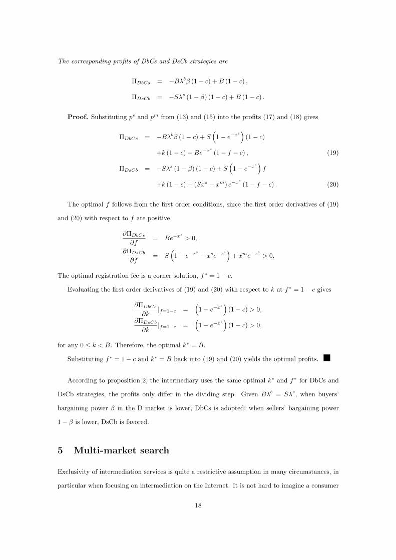
The corresponding profits of DbCs and DsCb strategies are

ΠDbCs = −Bλbβ (1− c) +B (1− c) ,

ΠDsCb = −Sλs (1− β) (1− c) +B (1− c) .

Proof. Substituting ps and pm from (13) and (15) into the profits (17) and (18) gives

ΠDbCs = −Bλbβ (1− c) + S(

1− e−xs)

(1− c)

+k (1− c)−Be−xs

(1− f − c) , (19)

ΠDsCb = −Sλs (1− β) (1− c) + S(

1− e−xs)f

+k (1− c) + (Sxs − xm) e−xs

(1− f − c) . (20)

The optimal f follows from the first order conditions, since the first order derivatives of (19)

and (20) with respect to f are positive,

∂ΠDbCs

∂f= Be−x

s

> 0,

∂ΠDsCb

∂f= S

(1− e−x

s

− xse−xs)

+ xme−xs

> 0.

The optimal registration fee is a corner solution, f∗ = 1− c.

Evaluating the first order derivatives of (19) and (20) with respect to k at f∗ = 1− c gives

∂ΠDbCs

∂k|f=1−c =

(1− e−x

s)

(1− c) > 0,

∂ΠDsCb

∂k|f=1−c =

(1− e−x

s)

(1− c) > 0,

for any 0 ≤ k < B. Therefore, the optimal k∗ = B.

Substituting f∗ = 1− c and k∗ = B back into (19) and (20) yields the optimal profits.

According to proposition 2, the intermediary uses the same optimal k∗ and f∗ for DbCs and

DsCb strategies, the profits only differ in the dividing step. Given Bλb = Sλs, when buyers’

bargaining power β in the D market is lower, DbCs is adopted; when sellers’ bargaining power

1− β is lower, DsCb is favored.

5 Multi-market search

Exclusivity of intermediation services is quite a restrictive assumption in many circumstances, in

particular when focusing on intermediation on the Internet. It is not hard to imagine a consumer

18

looking for some specific good will usually visit his favorite intermediation service providers first,

and if he is not satisfied, he might continue to search in his living city. This section is therefore

devoted to the analysis on how an intermediary works with non-exclusive intermediation being

possible. Under non-exclusive intermediation, buyers and sellers use the intermediary’s service as

well as search by themselves. We start with an adjustment on timing, then analyze two cases, one

with the C market opens first, and the other with the D market opens first.

Timing Non-exclusivity makes the operating time of the intermediary relevant. If the inter-

mediation operates before the D market, then buyers and sellers still hold their outside options

when participating in the C market. Therefore, if they are not matched at the intermediary, there

are still chances in the D market. In this way, there will be a substantial difference compared to

the exclusivity case, as will be shown in sections 5.2 and 5.3. In contrast, if the intermediation

operates after the D market closes, then by the time that the C market opens, all participating

buyers and sellers are those who are not matched in the D market. We essentially go back to a

exclusivity situation as will be shown in section 5.1. Instead of any specific sequence between the

C and D market, we allow the intermediary to choose its business hours. A comparison of the

two operating time shows that the intermediary would like to take the first moving advantage.

This partly explains why many online retailers are enthusiastic in making their websites fast and

easy to use, providing a wide range of information on the commodity, offering personalized service

such as special offer emails tailored to a customer’s interest, etc. These are to enhance customer

experiences, create loyalty and thus make the intermediary a first-mover.

Formally, the timing of events is as follows.

1. A competitive wholesale market opens where the intermediary stocks its inventory as a

middleman, denoted by k ∈ [0, B]. The wholesale market then closes.

2. The C and D retail markets open. The intermediary chooses the opening time, either before

or after the D market closes.

3. The intermediary announces a set of fees F ={f, gb, gs

}for the marketmaker sector and the

inventory k of the middleman sector, where the transaction fee f ∈ [0, 1− c], the registration

fees gb, gs ∈ [−1, 1].

4. Observing the fees and the inventory, buyers and sellers independently decide which mar-

19

ket(s) to participate in. If the C market opens first, individuals could attend the C market

and then the D market (if they are not matched in the C market), or ignore the C market

and only join the D market later. If the D market opens first, individuals could attend the

D market and then the C market (if they are not matched in the D market). Since the D

market is of free access, there is no reason to ignore the D market and only join the C market

later. Registration fees need to be paid in advance before entering the C market, whereas

entering the D market is free.

5. Matched pairs are formed in each market, and transactions are implemented.

5.1 The case where the D market opens first

Given the D market is of free access, all individuals attend it. After the matches in the D

market, there are B(1 − λb) buyers and S(1 − λs) sellers left unmatched. Since agents have lost

outside options, a slightly negative registration fee is enough to divide one type, gi = 0, i = B,S.

According to proposition 2, it is optimally for the intermediary to be a pure middleman, and

charge a monopolistic price pm = 1. The corresponding profit is B(

1− λb)

(1 − c). We will

compare this profit with that when the C market opens first and decide which opening time is

optimal for the intermediary in proposition 4.

5.2 The case where the C market opens first

In this subsection, we follow backward induction to solve the directed search equilibrium in the

second stage of the game, and the intermediary’s profit maximization problem in the first stage.

5.2.1 Second stage: the directed search equilibrium

We now consider the directed search equilibrium when the C market opens first. Under pessimistic

expectations, a profitable strategy for the intermediary must be a divide-and-conquer strategy.

This amounts to all buyers and sellers who participate in the C markets. Among a mass of B

buyers, Sxs will visit some independent sellers, and the rest xm will visit the middleman,

Sxs + xm = B. (21)

The equilibrium value of a buyer visiting an independent seller is

V b(s) = ηs (xs) (1− ps − f) + (1− ηs (xs))λbe−xs

β (1− c) . (22)

20

where ηs (xs) ≡ 1−e−xs

xs as defined before. This equation can be interpreted as follows. With a

chance of ηs (xs), the buyer is served and gets the value of the commodity after paying the price

ps and the transaction fee f . With a probability 1 − ηs (xs), the buyer will not be served. Still

he gets β (1− c) if he is matched in the D market with another seller who can’t trade in the C

market. This happens with a probability of λb (1− xsηs (xs)) = λbe−xs

.

Similarly, the equilibrium value of buyers visiting the middleman is

V b(m) = ηm (xm) (1− pm) + (1− ηm (xm))λbe−xs

β (1− c) . (23)

where ηm (xm) ≡ min{k,xm}xm is the serving probability at the middleman. With probability

ηm (xm), the buyer will be served and receives 1 − pm. In the equilibrium, a buyer should be

indifferent between visiting an independent seller or the middleman in the centralized market.

Thus, V b(s) = V b(m).

Consider the value of a seller. With probability xsηs (xs), the seller will be matched in the C

market and receives ps − c. With probability of (1− xsηs (xs))λs, the seller will not be matched

in the C market but be matched in the D market with another buyer. To eventually conclude a

transaction in the D market, the matched buyer must fail to trade in the C market, which happens

with probability ξ (xm, k), defined as

ξ (xm, k) ≡ 1−(xm

Bηm (xm, k) +

B − xm

Bηs (xs)

).

The expression in the brackets is the expected chance of a buyer to trade in the C market. In

particular, xm out of the B buyers are matched at the middleman, and the rest B − xm are

matched in the marketmaker sector. Summarizing all the elements yields the seller’s equilibrium

value

V s = xsηs (xs) (ps − c) + (1− xsηs (xs))λsξ (xm, k) (1− β) (1− c) .

Finally, the profits of the intermediary consists of two parts, platform fees and inventory profits,

Π (pm; k, F ) = Bgb + Sgs + Tf + xmηm (xm) pm − kc, (24)

where T is the expected amount of trades on the platform. Registration fees gb, gs are taken as

given at the moment.

Sellers Consider a deviating seller posting a price pd 6= ps. This seller is characterized by an

expected queue of buyers measured by xd 6= xs. The optimal price of this seller can be determined

21

by maximizing the expected profit,

V s =(

1− e−xd) (pd − c

)+ e−x

d

λsξ (xm, k) (1− β) (1− c) ,

subject to a market utility condition indicating that buyers are indifferent between visiting this

deviating seller and other sellers,

V b =1− e−xd

xd(1− pd − f

)+

(1− 1− e−xd

xd

)λbe−x

s

β (1− c) .

Each seller is infinitely small, and therefore can take V b as given.

To solve this problem, first substitute the price from the constraint into the objective to get

the expected profit of the deviating seller in terms of the arrival rate xd. Taking V b as given, the

optimal xd∗ satisfies the first order condition∂V s(xd∗)

∂xd= 0. The second order condition is satisfied.

In a symmetric equilibrium, all sellers have the same arrival rate xd∗ = xs. The equilibrium price

ps satisfies

ps − c = (1− βC) (v − f) + λsξ (1− β) (1− c) , (25)

where βC ≡ xse−xs

1−e−xs is the bargaining power for buyers induced by directed search equilibrium, and

v ≡[1− λbe−xsβ − λsξ (1− β)

](1− c) can be regarded as the total payoff that can be divided

by a buyer and a seller in the C market, taking into account their outside market values λbe−xs

β

and λsξ (1− β), respectively.

Inserting the equilibrium price ps (25) yields the equilibrium values of buyers and sellers

V b(s) = e−xs

(v − f) + λbe−xs

β (1− c) , (26)

V s =(

1− e−xs

− xse−xs)

(v − f) + λsξ (1− β) (1− c) . (27)

Finally, using equilibrium values V b(m) in (23), V b(s) in (26) and V b(s) = V b(m), the equilibrium

price pm can be written as

pm = 1− λbe−xs

β (1− c)− xme−xs

min {k, xm}(v − f) . (28)

Incentive constraints Because the intermediary opens first, agents know whether they are

matched in the I market before the D market opens. But even an agent is matched in the I

market, he might forgo this trading opportunity and continue to search in the coming D market.

For example, a matched seller will receive ps − c by trading on the I market platform, and his

expected value in the coming D market is λsξ (xm, k) (1− β) (1− c), thus the seller would indeed

22

to trade in the I market if and only if

ps − c ≥ λsξ (xm, k) (1− β) (1− c) .

Similarly, to have buyers trade in the I market ex post, prices must satisfy

1− pm ≥ λb (1− xsηs (xs))β (1− c) ,

1− ps − f ≥ λb (1− xsηs (xs))β (1− c) ,

where the first and the second condition correspond to a buyer visiting the middleman and the

platform, respectively.

Using expression (25) for ps and (28) for pm, the three incentive constraints can be simplified

to one restriction on f

f ≤ v ≡[1− λbe−x

s

β − λsξ (xm, k) (1− β)]

(1− c) . (29)

Basically, inequality (29) imposes an upper bound on the transaction fee that depends on the

outside option values of buyers (λbe−xs

β) and sellers (λsξ (xm, k) (1− β)). It differs from the

natural upper bound of 1− c as in the exclusivity case.

Intermediary We now turn to the intermediary’s pricing pm. With the one-to-one relationship

(28) between pm and xm, and taking intermediation fees and inventory as given, the intermediary’s

problem in the second stage is to choose the optimal xm, subject to the incentive constraint,

maxxm∈[0,B]

Π (xm; k, F ) = S(

1− e−xs)f + min {k, xm} pm (xm)− kc

s.t. f ≤ v. (30)

Problem (30) can be solved using the standard Kuhn-Tucker method as shown in lemma 4. The

intuition behind the lemma is exactly the same as behind lemma 2.

Lemma 4 Given B > 0, S > 0, f ∈ [0, 1− c] and k ∈ [0, B], the optimal expected queue of the

middleman satisfies xm = min {x̃m (f) , k} , where x̃m (f) ∈ (0, B] does not depend on k.

Finally, the directed search equilibrium analyzed so far is summarized in the following lemma.

Lemma 5 Given an announced set of fees, F = {f, gb, gs}, and inventory k, B > 0 buyers and

S > 0 sellers have decided to participate in the C market, a directed search equilibrium exists

23

and is unique. It is described by a queue of buyers at the middleman xm ∈ (0, B), a queue of

buyers at each seller xs ∈ (0, B/S), the equilibrium prices ps, pm ∈ (0, 1), and the value of buyers

V b ∈ (0, 1), of sellers V s ∈ (0, 1), and of the intermediary Π ∈ (0, B) satisfying (21), (24), (25),

(26), (27), (28), and lemma (4).

5.2.2 First stage: intermediation structure and fees

In this section, we study the determination on the intermediary’s optimal fees and inventory.

Concerning the divide and conquer strategy, the difference to exclusive service is that now any

negative registration fee ensures that individuals take the C market as the second home to cash

the subsidy, since they need not to give up the D market to do so. So attracting one side of the

market becomes less costly. By contrast, conquering the other side becomes more difficult, since

the conquered side still holds the trading opportunity in the D market.

The DsCb condition under non-exclusive service is

Ds: − gs ≥ 0,

Cb: V b − gb ≥ λbe−xs

β (1− c) .

The divide seller condition Ds tells us that the intermediary should provide a slightly negative

entrance fee so that all sellers will participate in and cash the fee even when there is no buyer at

all. The conquer buyer condition Cb thus extracts the surplus of buyers by giving them merely

the value of only attending the D market. Since matching is first implemented in the C market,

buyers devoted to the D market can only trade successfully with a probability of λbe−xs

, and thus

the value of the D market is λbe−xs

β (1− c). Similarly, the DbCs condition under non-exclusive

service is

Db: − gb ≥ 0,

Cs: V s − gs ≥ λsξ (xs, xm) (1− β) (1− c) .

Let’s first consider the relationship between xm and the optimal inventory. In particular,

whether the intermediary would like to hold more inventory than its queue length, k > xm. As

in section 3, the optimal behavior of the intermediary must be consistent. That is, the optimal

inventory is such that the intermediary can later accommodate exactly the same amount of buyers,

xm (k, f) = k. Less buyers than inventory (x̃m (f) < k) manifests an unnecessary spending on the

24

inventory. The intermediary gains a higher profit by reducing the redundant inventory. We thus

have the following lemma.

Lemma 6 The optimal inventory satisfies k ≤ x̃m (f).

Given xm = k, the accounting identity becomes

B = k + Sxs. (31)

The matching probability at the middleman becomes ηm = 1.

The intermediary’s problem in the first stage is to choose the optimal inventory k and trans-

action fee f to maximize

Π (k, F ) = Bgb + Sgs + S(

1− e−xs)f + k (pm (k, f)− c)

subject to incentive constraint (29) and divide-and-conquer conditions described above.

Applying V b(s) = V b(m), we have

pm (k, f)− c =(

1− λbe−xs

β)

(1− c)− e−xs

(v − f) .

Substituting the divide-and-conquer conditions yields registration fees under DbCs

gb = 0, gs =(

1− e−xs

− xse−xs)

(v − f) ,

and registration fees under DsCb

gs = 0, gb = e−xs

(v − f) .

To solve the problem, let’s start with the transaction fee. The intuition in previous sections

continues to hold. An increasing in f raises platform fees and price pm directly, but also reduces

buyers and sellers’ values and thereby reduces their registration fees. However, the overall effect is

positive since divide and conquer strategies only extract the value of one type, either that of the

buyers or sellers. The optimal f is ultimately bounded above, imposed by the incentive constraint

f = v.

To continue with the choice on k, insert the bounded f = v, the registration fees under either

divide and conquer strategy become zero, and the profits of DbCs and DsCb then become the

same,

Π (k) ={S(

1− e−xs)(

1− λbe−xs

β − λsξ (1− β))

+ k(

1− λbe−xs

β)}

(1− c) .

25

It is a sum of profits in two sectors, which again implies that the problem of choosing the optimal

inventory is essentially to allocate buyers between the two modes. Increasing inventory is equiva-

lent to increasing the fraction of middleman and decreasing the fraction of the platform, and vice

versa.

There are two concerns involved in choosing the relative sizes of the platform and the middle-

man. First, it follows from previous sections that the middleman mode offers a lower out-of-stock

risk, and a higher k creates more transactions. What’s new in the current setting is the outside

competition, represented by buyers and sellers’ decentralized market values. These outside val-

ues cap the intermediary’s price as stated in the incentive constraints, f ≤ v. Reflected in the

profit function, buyers’ outside value λbe−xs

β (1− c) is deprived from intermediary’s profit for

each transaction, whether it is on the platform or at the middleman, and sellers’ outside value

λsξ (xm, k) (1− β) (1− c) is deprived for each transaction of the platform. Notably, as the inter-

mediary moves towards a larger middleman sector (k increases), less sellers will be matched in

the C market due to the shrinking platform, more buyers will be matched in the C market by

trading with the middleman. Therefore, more sellers and less buyers are left to be available in the

D market. Accordingly, the buyers’ outside value increases and sellers’ outside value decreases.

When k is large, the former one is the main concern. The intermediary would have the incentive

to decrease k in order to lower the buyers’ outside value. In the following proposition, we show

that this competition effect is so strong that it overcomes the effect of the transaction efficiency

and yields an optimal inventory k∗ < B. We thus explained the endogenous choice of a hybrid

intermediation mode.

Proposition 3 With non-exclusivity, when the C market opens first, the intermediary’s optimal

strategy is to charge zero registration fees for buyers and sellers, the optimal transaction fee f∗ =

v (k∗), the optimal inventory is set to be strictly smaller than B, k∗ ∈ [0, B). In particular, when

1− λbe−BS β − e−BS v(B

S

)(1− β) + λb

(1− e−BS

)(1− e−BS − β

)≤ 0, (32)

the pure marketmaker mode (k∗ = 0) is optimal.

Proof. Given that

∂Π (k)

∂k=

−e−xsv + 1− λbe−xsβ − S(1−e−x

s)+k

S λbe−xs

β

+λb(1− e−xs

)2(1− β)

(1− c) ,

26

we have ∂Π(k)∂k |k=B = −BS λ

bβ (1− c) < 0. This shows k∗ < B. When ∂Π(k)∂k |k=0 ≤ 0 (which is

simplified to inequality (32) in the proposition), k∗ = 0. Since Π (k) is concave over the relevant

set of k,

∂2Π (k)

∂k2=

(−e−xs

Sv − 3λb

Se−x

s(

1− e−xs)− k

S2λbe−x

s

β

)(1− c) < 0 .

the second order condition holds.

If we set S = 1 − B, we can visualize inequality (32) in the space of(β,B, λb

), as shown in

figure ??. The shadowed region is the parameter set that yields k∗ = B. As one can see, this

happens when the mass of buyers B is small and the buyer’s outside option is large (λb and β are

of big values).

0.0

0.5

1.0

β

0.0

0.5

1.0

B

0.0

0.5

1.0

λb

Figure 2: Illustration of the parameter space (shadowed region) where pure marketmaker mode isoptimal

The explanation of proposition 3 is consistent with the rise of the online shopping and the

decline of brick and mortar stores. If we regard the decentralized market as the enormous tradi-

tional high street shops, and the centralized market as the online intermediary such as Amazon,

27

then we do see that the intermediary undercuts the price in the decentralized market to engage

customers in the model, which seems to fit the commonly held view that online intermediaries

benefit consumers by lowering prices. However, as is shown, the consumers are actually worse due

to the platform strategy. The decline of the high street shops reduces buyers’ market value, so

that the intermediary can eventually impose a even higher price. If one takes into account the

traditional store experiences, such as browsing and lingering in the bricks-and-mortar bookstores

or record shops, the utility decrease described by the model would only be a lower bound.

Next, we study the optimal inventory with regards to changes of the buyer’s bargaining power

β. When β increases, the buyers’ outside market value e−xs

λbβ (1− c) increases. This indicates

the effect of using the marketmaker mode to lower buyers’ outside value becomes more important.

As a result, the optimal k should decrease.

Corollary 1 (Comparative statics) An increase in buyer’s bargaining power β in the decen-

tralized market leads to a lower optimal inventory k∗.

To compare whether the intermediary chooses to move first, we evaluate the first-move profit

at a suboptimal inventory level of k = B. This yields a profit of B(

1− λbβ)

(1− c), which is

strictly larger than that when the intermediary opens after the D market B(

1− λb)

(1− c). We

conclude that the intermediary would optimally take the ”first move advantage”.

Proposition 4 With non-exclusive intermediation, the intermediary optimally opens the C mar-

ket before the D market, and uses the optimal strategy characterized in proposition 3.

6 Discussion and extensions

This part discusses the implications of the previous results and some extensions.

Efficiency and welfare The social optimum is achieved when all buyers are matched with

suppliers, either independent sellers or the middleman. Apparently, when the inventory of the

middleman is set at k = B, all buyers are matched. As long as the marketmaker mode is employed,

the directed search friction renders a less efficient allocation. This implies that the optimal strategy

of the intermediary is, however, not optimal for society. Given our analysis before, the reason lies in

28

the competition from the outside market. The incentives for the intermediary to be a marketmaker

is to absorb sellers from the outside market and thus reduce buyers’ outside value. In other words,

it is market competition, rather than market power, that brings efficiency and welfare loss. This

conclusion is at odds with the common wisdom.

In terms of welfare of buyers and sellers, we find that under exclusivity, buyers and sellers

get their expected values in the decentralized market, the same as when there is no intermediary.

Under non-exclusivity, the intermediary attracts transactions using a platform, which lowers the

buyer and seller’s expected values. They get even less than that without the intermediary.

Mortenson and Pissarides type matching functions in the D market Our conclusion

holds for a very general setting of the D market. Instead of a linear matching function, assume

the flow of contacts between sellers and buyers in the D market is given by a matching technology

M = M(BD, SD

),

where BD and SD denote the amount of buyers and sellers that actually participate in the D

market. It is standard to assume the function M is continuous, nonnegative, with M(0, SD

)=

M(BD, 0

)= 0 for all

(BD, SD

).

Define the matching probabilities λb(BD, SD

)=

M(BD,SD)BD

and λs(BD, SD

)=

M(BD,SD)SD

for buyers and sellers, respectively. Under exclusive intermediation, we have the same conclusion

with new defined matching probabilities λb = λb (B,S), λs = λs (B,S).

With non-exclusive intermediation, under a fairly reasonable condition that λb(BD, SD

)is

decreasing in BD and increasing in SD, we can show our conclusion holds. If the C market opens

first, then the matching in the D market depends on how many buyers and sellers are not matched

in the C market. In particular, min {k, xm} + S(1− e−xs

)buyers and S

(1− e−xs

)sellers are

matched in the C market, and thus

BD = B −min {k, xm} − S(

1− e−xs),

SD = S − S(

1− e−xs).

Following the same derivation as in section 5, we have the intermediary’s profits

Π (k) =

S(1− e−xs

) (1− λb

(BD, SD

)β − λs

(BD, SD

)(1− β)

)+k(

1− λb(BD, SD

)β)

(1− c) ,

29

where the first item in the brace is the platform profit, and the second item is the middleman

profit. The first order derivative with respect to inventory is

∂Π (k)

∂k=

−e−xs

(1− λb

(BD, SD

)β − λs

(BD, SD

)(1− β)

)+S

(1− e−xs

)(1− ∂λb(BD,SD)

∂k β − ∂λs(BD,SD)∂k (1− β)

)+(

1− λb(BD, SD

)β)− k ∂λ

b(BD,SD)∂k β

(1− c) .

Evaluating this derivative at k = B drops all items in the brace except the last one,

∂Π (k)

∂k|k=B = −B

∂λb(BD, SD

)∂k

β (1− c) .

To make a pure middleman model non-optimal (∂Π(k)∂k |k=B < 0), we need

∂λb(BD,SD)∂k > 0, which

can be decomposed into two parts,

∂λb(BD, SD

)∂k

=∂λb

(BD, SD

)∂BD

∂BD

∂k+∂λb

(BD, SD

)∂SD

∂SD

∂k.

Since ∂BD

∂k < 0 and ∂SD

∂k > 0, we need∂λb(BD,SD)

∂BD≤ 0,

∂λb(BD,SD)∂SD

≥ 0,∂λb(BD,SD)

∂BD×∂λ

b(BD,SD)∂SD

6= 0.

Heterogenous search costs In the real world, individuals have different search costs in the

outside market. This may be due to many factors, such as shopping experiences, living locations,

whether the agent is a local resident or a foreigner, etc. In our model, we can also capture this

by assuming agents sample a search cost from a distribution. This gives more flexibility for the

intermediary. In particular, besides divide and conquer strategies, there is a new strategy where

the intermediary just sets a high price to extract all trade surplus and waits for the high search cost

agents to arrive. The flip side is that such a strategy would disappear in the non-exclusivity case.

To see why, consider a pure marketmaker. In this scenario, dividing an agent is free by simply

giving the agent a small positive value. Thus, the low search cost agents can also be divided.

Moreover, if these low search cost agents are not matched in the D market, their outside market

value becomes zero, and they would like to trade in the C market. This means, there exists a

divide and conquer strategy, where the intermediary serves as the second source for low search

cost agents that strictly dominates the proposed new strategy. Therefore, our modeling doesn’t

lose much in this aspect.

30

7 Conclusion

This paper presents a theory of a hybrid intermediary using a standard directed search approach

within a two-sided markets framework. When the intermediary works as a marketmaker, it orga-

nizes a marketplace where price and capacity information spreads efficiently and only coordination

frictions exist, i.e. search is directed. When the intermediary works as a middleman, it purchases

a large inventory from a competitive wholesale market and resells to buyers. Middleman’s inven-

tory can provide buyers with immediate service under market frictions, thereby it increases the

number of transactions.

We explored whether and when the mixture of the two modes, the marketmaking middleman,

would be optimal, under both single-market and multiple-market search technologies. In the

former case, we find the intermediary’s optimal mode is to be a pure middleman in order to

create as many trades as possible. In the latter case, due to competition from other retailers (the

decentralized market in the model), the intermediary has to slash retail price in order to compete

with the outside market. Rather than going to a cut-throat price war, the intermediary’s best

response is to have rivals join its business and become a marketmaking middleman.

This article considers only the monopoly case. For future research, it would be interesting to

also study the oligopoly case. In particular, we could check whether our conclusion still holds

when another marketmaking middleman is explicitly characterized. Since our model provides a

microfoundation for the mixture of middleman mode and marketmaker mode, it can be potentially

extended to discuss more specific intermediaries such as marketmakers in financial markets.

31

8 Appendix

8.1 Proof of lemma 2

The intermediary aims to maximize Π (pm; k, f). Substituting pm = 1− xm

min{k,xm}e−xs (1− f − c) gives

Π (xm; k, f) = Bgb + Sgs + S(

1− e−xs)f + min {k, xm} − xme−x

s

(1− f − c)− kc.

To find the optimal xm, consider two cases: xm > k or xm ≤ k.When xm > k, the first order derivative is

∂Π (xm; k, f)

∂xm= −e−x

s

f − e−xs

(1− f − c)− xme−xs

S(1− f − c) < 0,

thus the optimal xm ≤ k.When xm ≤ k, the first order derivatives is

∂Π (xm; k, f)

∂xm= 1− e−x

s

(1− c)− xm

Se−x

s

(1− f − c) .

∂Π(xm;k,f)∂xm

= 0 gives x̃m (f) .

Notice ∂Π(xm;k,f)∂xm

|xm=0 = 1− e−BS (1− c) > 0, thus x̃m (f) > 0. But

∂Π (xm; k, f)

∂xm|xm=B = c− B

S(1− f − c) ≷ 0,

depending on f .The second order condition is satisfied since Π (xm; k, f) is concave in xm,

∂2Π (xm; k, f)

∂ (xm)2 = − 1

Se−x

s

(1− c)− S + xm

S2e−x

s

(1− f − c) < 0.

8.2 Proof of lemma 4

Substitute pm (xm) into the profit function, we have the problem as

maxxm

Π (xm; k, F ) = S(

1− e−xs)f + min {k, xm}

(1− λbe−x

s

β (1− c))− xme−x

s

(v − f)

s.t. f ≤ v,

where v ≡(

1− λbe−xs

β − λsξ (1− β))

(1− c) , and ξ = 1− min{k,xm}B

− SB

(1− e−x

s).

First, we show that any xm > k can’t be optimal.Suppose xm > k and the incentive constraint is binding (f = v), then set the Lagrangian as

L = S(

1− e−xs)f + k

(1− λbe−x

s

β (1− c))− xme−x

s

(v − f) + µ (v − f) ,

where µ > 0. However,

∂L∂xm

= −e−xs

f − k

Sλbe−x

s

β (1− c)− µλbe−x

s

B(1− c) < 0.

Suppose xm > k and the incentive constraint is not binding (f < v). We can derive the first orderderivative

∂Π (xm; k, F )

∂xm= −e−x

s

f −(

1 +xm

S

)e−x

s

(v − f)

− kSλbe−x

s

β (1− c) +xme−x

s

Bλbe−x

s

(1− c) .

If ∂Π(xm;k,F )∂xm

< 0 for ∀xm ∈ (k,B], then we can immediately conclude any xm > k can’t be optimal.

If ∂Π(xm;k,F )∂xm

> 0 for ∀xm ∈ (k,B], we must have the optimal xm = B. But a marginal increase in k

at the first stage of the game raises profits by(1− λbβ

)(1− c) till k = xm. A contradiction.

32

If ∃x̆m ∈ (k,B] such that ∂Π(xm;k,F )∂xm

|x̆m = 0, then optimality can only be achieved at such x̆m. Thesecond order derivative follows that

∂2Π (xm; k, F )

∂xm2|x̆m =

1

S

∂Π (xm; k, F )

∂xm|x̆m + φ (x̆m)

where

∂Π (xm; k, F )

∂xm|x̆m =

{−e−x

s

f − kSλbe−x

s

β (1− c)− e−xs

(v − f)

− x̆m

Se−x

s

(v − f)− x̆me−xs ∂v∂xm|x̆m

},

φ (x̆m) ≡

{−e−x

s ∂v∂xm|x̆m − 1

Se−x

s

(v − f)− x̆m

Se−x

s ∂v∂xm|x̆m

−x̆me−xs(

∂v∂xm|x̆m + ∂2v

∂xm2 |x̆m) }

,

∂v

∂xm|x̆m = −λ

b

Se−x

s

(1− c) , ∂2v

∂xm2|x̆m = − λ

b

S2e−x

s

(1− c) .

Given ∂Π(xm;k,F )∂xm

|x̆m = 0, we have

1

Se−x

s

(v − f) =1

S

{−e−x

s

f − kSλbe−x

s

β (1− c)− x̆

m

Se−x

s

(v − f)− x̆me−xs ∂v∂xm|x̆m

}≤ − 1

Sx̆me−x

s ∂v

∂xm|x̆m ,

thus ∂2Π(xm;k,F )

∂xm2 |x̆m = φ (x̆m) > 0. Thus the second order condition is not satisfied.

Second, we consider the problem when xm ≤ k. The Lagrangian becomes

L = S(

1− e−xs)f + xm

(1− λbe−x

s

β (1− c))− xme−x

s

(v − f) + µ (v − f) .

Since there is no k in this expression, the solution should only depends on f and other parameters, denotedas x̃m (f).

Sum up the analysis, we conclude the optimal queue xm at the second stage is

xm (k, f) = min {x̃m (f) , k} .

8.3 Proof for Corollary 1

We first deal with the corner solutions. If k∗ = 0, then increase in β certainly won’t decrease the optimalinventory as it is on the lower bound.

Turn to the interior solution k∗ ∈ (0, B). Define F (k, β) = 11−c

∂Π∂k

(k, β) = 0. Given ∂k∂β

= −∂F (k,β)∂β

∂F (k,β)∂k

,

and ∂F (k,β)∂k

< 0, to show ∂k∂β

< 0, we only need to prove ∂F (k,β)∂β

< 0. This is the case,

∂F (k, β)

∂β=

1

1− c∂2Π

∂β∂k(k, β)

= −e−xs

λsξ − λb(

1− e−xs)−S(

1− e−xs)

+ k

Sλbe−x

s

− λb(

1− e−xs)2

< 0.

33

References

[1] Acemoglu, D. and R. Shimer, (1999), Holdup and Efficiency with Search Frictions, Interna-

tional Economic Review, 47, 651-699.

[2] Albrecht, J., P. Gautier, and S. Vroman (2006), Equilibrium Directed Search with Multiple

Applications, Review of Economic Studies, 73 (4), 869-891.

[3] Armstrong, M. (2006), Competition in Two-Sided Markets, RAND Journal of Economics, 37

(3), 668-691.

[4] Baye, M., and J., Morgan (2001), Information Gatekeepers on the Internet and the Compet-

itiveness of Homogeneous Product Markets, American Economic Review, 91 (3), 454-74.

[5] Biglaiser, G. (1993), Middlemen as Experts, RAND Journal of Economics, 24 (2), 212-223.

[6] Burdett, K., S. Shi, and R. Wright (2001), Pricing and Matching with Frictions, Journal of

Political Economy, 109 (5), 1060-1085.

[7] Caillaud, B., B. Jullien (2001), Software and the Internet Competing Cybermediaries, Euro-

pean Economic Review, 45, 797-808.

[8] —————————— (2003), Chicken and Egg: Competition among Intermediation Service

Providers, RAND Journal of Economics, 34 (2), 309-328.

[9] Chen, K. -P and Y. -C. Huang (2012), A Search-Matching Model of the Buyer-Seller Plat-

forms, CESifo Economic Studies, 58 (4), 626-49.

[10] Duffie, D., N. Garleanu, and L. H. Pedersen (2005), Over-the-Counter Markets, Econometrica,

73 (6), 1815-1847.

[11] Edelman, B. and J. Wright (2015), Price Restrictions in Multi-sided Platforms: Practices

and Responses, Harvard Business School NOM Unit Working Paper No. 15-030.

[12] Fingleton, J., (1997), Competition among middlemen when buyers and sellers can trade

directly, Journal of Industrial Economics 45 (4), 405-427.

[13] Galeotti, A. and J.L. Moraga-Gonzalez (2009), Platform Intermediation in a Market for

Differentiated Products, European Economic Review, 53 (4), 417-428.

[14] Gehrig, T. (1993), Intermediation in Search Markets, Journal of Economics and Management

Strategy 2 (1), 97-120.

[15] Guerrieri, V., R. Shimer and R. Wright, (2010), Adverse Selection in Competitive Search

Equilibrium, Econometrica, 78, 1823-1862.

[16] Hagiu, A. (2006), Pricing and Commitment by Two-Sided Platforms, RAND Journal of

Economics, 37 (3), 720-737.

34

[17] Hagiu, A. and J. Wright (2013), Do You Really Want to Be an eBay?, Harvard Business

Review, 91 (3), 102–108.

[18] ——————————— (2014), Marketplace or Reseller?, Management Science, 61 (1), 184

- 203.

[19] Hendershott, T. and A.J. Menkveld (2014), Price Pressures, Journal of Financial Economics,

114 (3), 405-423.

[20] Holzner, C. and M. Watanabe (2015), Labor Market Equilibrium with Public Employment

Agency, Tinbergen Institute working paper.

[21] Johri, A. and J. Leach (2002), Middlemen and the Allocation of Heterogeneous Goods, In-

ternational Economic Review 43 (2), 347-361.

[22] Lagos, R., and G. Rocheteau (2007), Search in Assets Markets: Market Structure, Liquidity,

and Welfare, American Economic Review, 97 (2), 198-202.

[23] ————————————— (2009), Liquidity in Asset Markets With Search Frictions,

Econometrica, 77 (2), 403-426.

[24] Li, Y. (1998), Middlemen and Private Information, Journal of Monetary Economics, 42 (1),

131-159.

[25] Loertscher, S. (2007), Horizontally Differentiated Market Makers, Journal of Economics and

Management Strategy, 16 (4), 793-825.

[26] Masters, A. (2007), Middlemen in Search Equilibrium, International Economic Review, 48

(1), 343-362.

[27] Moen, E. R. (1997), Competitive Search Equilibrium, Journal of Political Economy, 105,

385-411.

[28] Nocke, V., Peitz, M. and Stahl, K. (2007), Platform Ownership. Journal of the European

Economic Association, 5 (6) 1130–1160.

[29] Peters, M., (1991), Ex Ante Pricing in Matching Games: Non Steady States, Econometrica,

59, 1425-1454.

[30] Peters, M., (2001), Limits of Exact Equilibria for Capacity Constrained Sellers with Costly

Search, Journal of Economic Theory, 95, 139-168.

[31] Rochet, J.-C. and J. Tirole (2003), Platform Competition in Two-Sided Markets. Journal of

the European Economic Association, 1(4), 990-1029.

[32] ———————————— (2006), Two-Sided Markets: A Progress Report, Rand Journal

of Economics, 37 (3), 645-667.

[33] Rubinstein, A., and A. Wolinsky. (1987), Middlemen, Quarterly Journal of Economics, 102

(3), 581-594.

35

[34] Rust, J., and R., Hall. (2003), Middlemen versus Market Makers: A Theory of Competitive

Exchange, Journal of Political Economy, 111 (2), 353-403.

[35] Rysman, M. (2009), The Economics of Two-Sided Markets, Journal of Economic Perspectives,

23 (3), 125-143.

[36] Shevichenko, A. (2004), Middlemen, International Economic Review 45 (1), 1-24.

[37] Spulber, D.F. (1996), Market Making by Price Setting Firms, Review of Economic Studies

63 (4), 559-580.

[38] —————— (1999), Market Microstructure, Cambridge.

[39] Stahl, Dale O. (1988), Bertrand Competition for Inputs and Walrasian Outcomes, American

Economic Review, 78 (1), 189-201.

[40] Watanabe, M. (2010), A Model of Merchants, Journal of Economic Theory, 145 (5), 1865-

1889.

[41] ——————— (2013), Middlemen: A Directed Search Equilibrium Approach, VU Univer-

sity Amsterdam and Tinbergen Institute working paper.

[42] Weyl, G. (2010), A Price Theory of Multi-Sided Platforms, American Economic Review, 100

(4), 1642-72.

[43] Wong, Y. and R. Wright (2014), Buyers, Sellers and Middlemen: Variations on Search-

Theoretic Themes, International Economic Review 55 (2), 375-397.

[44] Yavas, A. (1994), Middlemen in Bilateral Search Markets, Journal of Labor Economics, 12(3),

406-429.

[45] ————— (1996), Search and Trading in Intermediated Markets, Journal of Economics &

Management Strategy, 5(2), 195-216.

36