1

Markets, transportation infrastructure and food prices in Nepal

Gerald Shively (contact author) Department of Agricultural Economics

Purdue University West Lafayette, IN 47907

shivelyg@purdue.edu (765) 494-4218 (voice) (765) 494-9176 (fax)

Ganesh Thapa

International Food Policy Research Institute Kathmandu, Nepal

thapaganesh@gmail.com

Forthcoming in the American Journal of Agricultural Economics ABSTRACT. We study transportation infrastructure and food markets in Nepal over the period 2002 to 2010, combining monthly price data from 37 local and regional markets and 7 Indian border markets. We use a series of autoregressive models to study price determination, spatial and temporal price transmission, and price variance. We account for district-level agricultural production, correcting for bi-directional causality between output and prices using ground station rainfall data. In addition, to test hypotheses regarding the importance of transportation infrastructure we incorporate information on road and bridge density and fuel costs. For both rice and wheat, we find strong evidence of local price intertemporal carryover and very weak evidence of price transmission from regional, central and border markets to local markets, suggesting very low degrees of market integration. Fuel costs are positively correlated with food prices, and road and bridge density are negatively correlated with prices. We find evidence of asymmetric effects: positive price shocks are correlated with higher subsequent price volatility compared with negative price shocks of similar magnitude. Roads and bridges are important for moderating price levels and price volatility in Nepal’s rice and wheat markets, explaining roughly half of the spatial and temporal variation in price mark-ups between regional and local markets. Key words: bridges, food prices, markets, rice, roads, wheat, Nepal JEL codes: Q02; Q11; R40

Authors are listed alphabetically. Support for this research was provided by the Feed the Future Innovation Lab for Nutrition, which is funded by the United States Agency for International Development. The opinions expressed herein are those of the authors and do not necessarily reflect the views of the sponsoring agency. We thank two anonymous reviewers and Molly Brown, Jake Ricker-Gilbert and Raymond Florax for helpful suggestions. In Nepal, Senior Agriculture Officer Mr. Bhojraj Sakot and Plant Protection Officer Mr. Manoj Pokhrel were instrumental in facilitating access to data. A data and model appendix as well as an online appendix of supporting information accompany this article.

2

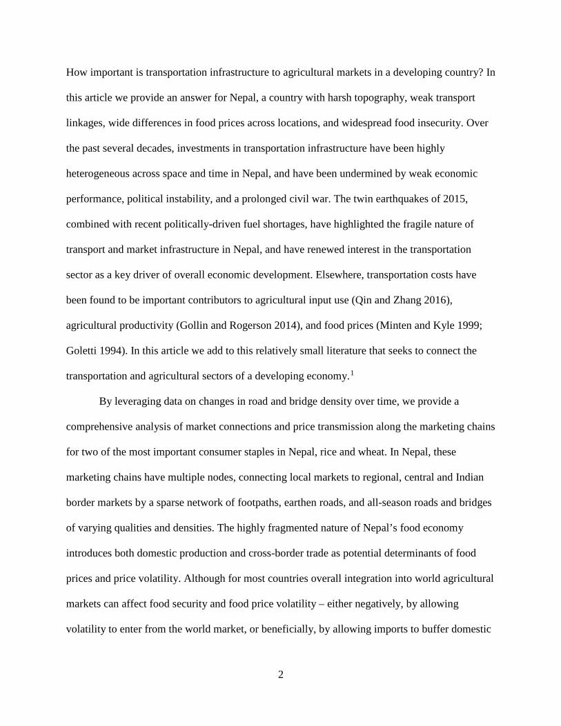
How important is transportation infrastructure to agricultural markets in a developing country? In

this article we provide an answer for Nepal, a country with harsh topography, weak transport

linkages, wide differences in food prices across locations, and widespread food insecurity. Over

the past several decades, investments in transportation infrastructure have been highly

heterogeneous across space and time in Nepal, and have been undermined by weak economic

performance, political instability, and a prolonged civil war. The twin earthquakes of 2015,

combined with recent politically-driven fuel shortages, have highlighted the fragile nature of

transport and market infrastructure in Nepal, and have renewed interest in the transportation

sector as a key driver of overall economic development. Elsewhere, transportation costs have

been found to be important contributors to agricultural input use (Qin and Zhang 2016),

agricultural productivity (Gollin and Rogerson 2014), and food prices (Minten and Kyle 1999;

Goletti 1994). In this article we add to this relatively small literature that seeks to connect the

transportation and agricultural sectors of a developing economy.1

By leveraging data on changes in road and bridge density over time, we provide a

comprehensive analysis of market connections and price transmission along the marketing chains

for two of the most important consumer staples in Nepal, rice and wheat. In Nepal, these

marketing chains have multiple nodes, connecting local markets to regional, central and Indian

border markets by a sparse network of footpaths, earthen roads, and all-season roads and bridges

of varying qualities and densities. The highly fragmented nature of Nepal’s food economy

introduces both domestic production and cross-border trade as potential determinants of food

prices and price volatility. Although for most countries overall integration into world agricultural

markets can affect food security and food price volatility – either negatively, by allowing

volatility to enter from the world market, or beneficially, by allowing imports to buffer domestic

3

supply shocks – Nepal is relatively isolated from world markets. Because it is landlocked, with a

formidable northern border crossing to Tibet and a controlled and highly politicized southern

border with India, local food security is quite sensitive to internal production and trade. If

Nepal’s local markets are not well connected to regional and border markets, and if those same

local markets are characterized by insufficient production and storage, high price volatility and

incomplete price transmission are likely to prevail. Under such conditions, one might

hypothesize, as we do here, that isolated markets are not likely to receive either price signals or

food shipments in a timely fashion, and that high transportation and storage costs will discourage

traders from engaging in the kinds of spatial and temporal arbitrage that improve market

integration. For these reasons, Nepal is an excellent case for investigating the importance of

transportation to agricultural prices. Below, we empirically test several hypotheses, including a

conjecture that higher road and bridge densities at the district level result in lower prices, lower

price volatility, and reduced transport costs. We also test whether fuel costs are positively

correlated with food prices and food price volatility, and measure their contribution to price

differences across locations and time. A key innovation in our approach is to incorporate

multiple levels of price-to-price transmission effects simultaneously. That is, contemporaneous

and lagged values of regional, border and central market prices are all included in the model for

monthly local prices. Such an approach obviously raises conceptual and statistical concerns

regarding multicollinearity among these various prices, an issue that we address by comparing

results from models in which regional, border and central market prices are treated as alternative

exogenous prices.

To the best of our knowledge, no previous studies – whether in Nepal or elsewhere –

have examined econometrically the connections between road and bridge infrastructure and food

4

prices. Our findings have implications not only for Nepal, but also for other settings where local

markets are fairly isolated, either by policy or by structure and geography. Our interest in food

prices and food price volatility is motivated by the large catalog of research demonstrating that

poor consumers can be adversely affected by increases in food prices (Alem and Soderbom

2011; Andreyeva et al. 2010; Bouis 2008; Deaton 1989; Hawkes 2012; Timmer 1989; Von

Braun 2008). Higher food prices undermine expenditures on nutrition-sensitive basic needs such

as health care and education (FAO et al. 2011); have been linked to the worsening of child health

and nutrition outcomes (Anriquez et al. 2013; Grace et al. 2014; Lavy et al. 1996; Thomas et al.

1992); and have been implicated in a range of negative social and non-nutritional outcomes

(Swan et al. 2009; Hadley et al. 2012), including social unrest (Bellemare 2014).2 Food price

volatility is also of concern. Large unexpected price fluctuations have been identified as a major

threat to food security in developing countries, especially where there is an underlying lack of

diet diversity (FAO 2010a). Price variability has been shown to have a negative effect on a range

of household welfare indicators (Cummings 2012; Dawe and Timmer 2012; Bellemare et al.

2013; Akter et al. 2014), and Kharas (2011) argues that, by creating economic and political

turbulence, price volatility jeopardizes long run social stability. Using data from Ghana, Shively

(2001) demonstrates that high price volatility raises the cost of stockholding as much as four-

fold, reducing incentives for traders and undermining market performance itself.

Given the widespread importance of food prices to nutritional outcomes in developing

countries, as well as a specific recognition of the long-standing economic, political and

environmental challenges facing Nepal, it is somewhat surprising that relatively little attention

has been devoted to the study of agricultural markets and prices in Nepal. Before the earthquakes

of early 2015, problems with food distribution were already widespread and the cost of

5

transportation was high, a situation often attributed to harsh topography and the isolation of

food-deficit regions (NAPMDD 2010; NMOAD 2012). The 2015 earthquakes have further

complicated the situation and underscored that little is formally known about agricultural price

transmission in Nepal. Most studies of Nepal’s agricultural markets to date have been highly

descriptive in nature (e.g. WFP/FAO 2007; Agostinucci and Loseby 2008; WFP/NDRI 2008;

FAO 2010b). A small number of price studies have employed econometric techniques (see

Sanogo 2008; Sanogo and Amadou 2010; Shrestha 2013), but few have focused

comprehensively on agricultural price transmission. Moreover, all past studies for Nepal use

relatively short price series and an extremely limited set of covariates, making it difficult to draw

strong inferences from the findings. We rectify these shortcomings below.

Empirical strategy

Our empirical approach builds upon price-focused models of commodity trade. Early empirical

models testing the law of one price in this way include Blyne (1973), Cummings (1967) and

Harriss (1979). Conceptually, whenever the price of a commodity in one market exceeds the

price of the same commodity in another market by more than the cost of transportation and

marketing, traders have an opportunity to engage in spatial arbitrage until prices converge,

thereby restoring spatial equilibrium (Ravallion 1986; Goodwin et al. 1990; Sexton et al. 1991;

Badiane and Shively 1998). Models in which market segmentation is related to transfer cost

thresholds were introduced by Baulch (1997) and Goodwin and Piggott (2001). Myers and Jayne

(2012) and Burke and Myers (2014) allow for threshold effects stemming from trade volume.

The assumption in all of these models is that suppliers and traders in regional and transit hubs

supply grain to various markets, adapting their marketing strategies to target destinations where

6

there is the greatest arbitrage opportunity. Temporary equilibriums and shortages lead traders to

shift their short-term focus among different areas and nodes. When markets are well connected

and when price signals are completely transmitted among markets, temporary disequilibria are

infrequent and quickly resolved. When information and products do not flow quickly or easily,

disequilibria may persist, suggesting potential pathways to improving overall welfare by raising

prices for producers, lowering prices for consumers, or both.3 Our innovation and contribution is

to incorporate multiple levels of price-to-price transmission effects simultaneously, whilst

explicitly accounting for market-specific factors that affect transfer costs.

Figure 1 illustrates the current market structure in Nepal and highlights the importance of

hubs located in the Terai as suppliers and transshipment points to the rest of the country. To

provide some sense of the heterogeneity in transportation infrastructure across space and time in

Nepal, figure 2 charts changes in transportation density in three representative districts of the

country: Jumla, located in the mountains; Kaski, in the middle hills; and Mahottari, in the Terai

(the plains bordering India). Largely because of low population density and a high cost of road

construction in the hills and mountains, in past decades the Terai has been given priority for road

and bridge construction (time paths of road construction in these districts is provided in

Appendix figure A1). More recently, the government has begun to boost investment in road and

bridge construction in the hills and mountains, but many remote districts remain inaccessible.4

As recently as 2010, 15 of 75 districts in the country were not road connected (FAO 2010c), and

as of 2015, Humla and Dolpa districts remained unconnected by roads to other parts of the

country. In many locations, several hours or days of road travel are required to reach the district

headquarters (CBS 2011). In 2005, it was estimated that more than a quarter of all households in

Nepal had to walk for at least eight hours to reach a road (FAO 2010c). In remote locations,

7

goods are often either airlifted or carried by mules or porters, adding substantially to the price of

final goods, especially during some periods of the year.

Roads and bridges, of course, are only one element contributing to transportation costs.

Another important component is fuel. Nepal imports all of its required refined oil from India via

the Nepal Oil Corporation Limited (NOC), a state-owned trading company that is solely

responsible for importation, transportation, storage, and distribution of petroleum products.

Although fuel prices in Nepal are not directly determined by the international market, increases

in international fuel prices are usually passed through to domestic consumers by the NOC.

Although petroleum products are heavily subsidized, between 1986 and 2013 the nominal diesel

price in Nepal increased nearly ten-fold, and spiked several times (Appendix figure A2).

To quantify the transmission of price signals and test the importance of transportation

infrastructure to food prices, we begin with Ravillion’s (1986) model. We make two fundamental

modifications. First, instead of focusing on a single market, we use a panel of local markets. We

connect each local market to its (a) Nepal-India border market (b) regional market and (c) central

market. Second, in contrast to studies which treat a primary supply location as the central market,

we assume that Nepal’s central market is Kathmandu. We reason that because approximately

10% of Nepal’s population lives in Kathmandu (NPHC 2011) and because Kathmandu’s demand

largely determines the position of the national demand curve (WFP/FAO 2007), demand from

the Kathmandu valley likely plays a key role in setting prices at the margin.

With Nepal’s market structure in mind, we define local markets as those small and

locally important trading centers that are located (mainly) in food deficit districts of the country.

These markets receive inflows of foods via border and regional markets. Regional markets are

located in districts with high production potential, storage facilities, and comparatively good

8

transportation links to other parts of the country. Border markets connect Nepal with India.5 The

central market for all local markets in Nepal is the capital, Kathmandu. Local food prices are

expected to depend on local supply, and to be influenced through trade by prices in regional,

central and border markets.6 We focus on 28 local markets with fairly complete time series for

rice and wheat prices. These markets are typical, but we make no strong claims regarding their

overall representativeness for Nepal.

Figures 3-5 display how the border (panel A), regional (B), and central (C) market prices

move with local market prices. Time trends for these prices are displayed in panel D of each

figure. Prices in Nepal are usually higher than in border markets and are widely assumed to be

influenced by Indian market prices. The NRB (2007), in fact, argues that food prices in Nepal are

determined by India, a conjecture we reject below. Figures 3A-5A show that border market

prices are positively correlated with local agricultural prices in the hills and Terai (Kaski and

Mahottari) but not the mountains (Jumla).

All of the regional markets are located in the Terai. We expect them to play an important

role in stabilizing food prices country-wide by providing storage, spatial and temporal arbitrage,

and intermediary activity for imports from India (Action Aid Nepal 2006). One might reasonably

expect supply shocks affecting regional markets to be transmitted to local markets. For example,

figures 3B to 5B illustrate that rice prices in the hills and Terai move closely with prices in their

corresponding regional markets. Similarly, figures 3C-5C show that the same prices are

positively correlated with the central market price.

With the forgoing definitions of markets in mind, we model the local market price as:

9

(1) Pilt = αi0 + αi1T + αi2M + αi3Y + αi4L + γiPilt−1 + ��βik

3

k=1

Pikt−j

1

j=0

+ 𝛉𝛉′𝐃𝐃 + 𝛅𝛅′𝐒𝐒 + ϑiEt + µilt

where 𝑃𝑃𝑖𝑖𝑖𝑖𝑖𝑖 represents the retail price for commodity i in market l at time t; 𝑇𝑇 is a unit-step

(monthly) time trend;. 𝑀𝑀, 𝑌𝑌 and 𝐿𝐿 are month, year, and location (agro-ecology) fixed effects;

𝑃𝑃𝑖𝑖𝑖𝑖𝑖𝑖−𝑗𝑗 is the price observed for commodity i in companion market k (either regional, central or

border) at time t, with lag j. Here 𝛼𝛼is, 𝛾𝛾𝑖𝑖,𝛽𝛽𝑖𝑖𝑖𝑖, 𝜽𝜽, 𝜗𝜗𝑖𝑖 and 𝜹𝜹 are parameters to be estimated. The

error term, 𝜇𝜇𝑖𝑖𝑖𝑖𝑖𝑖, is assumed to be independently and identically distributed across the

observations. Parameters 𝛽𝛽𝑖𝑖𝑖𝑖 and 𝛾𝛾𝑖𝑖 are coefficients for spatial market price transmission and

auto-regressive lags, respectively; D and S are column vectors representing demand and supply

shifters and 𝐸𝐸𝑖𝑖 is the exchange rate, which we assume can influence both demand and supply. D

includes annual district population. S includes infrastructure (roads and bridges), fuel prices, and

agricultural production.

Directly incorporating agricultural production as an independent variable in equation (1)

is problematic because prices can both influence and be influenced by output. To address the

endogeneity issue introduced by this bi-directionality, we predict the quantity harvested (𝑄𝑄𝑖𝑖𝑖𝑖𝑖𝑖)

using a time trend (𝑇𝑇), rainfall (𝑅𝑅𝑖𝑖𝑖𝑖𝑖𝑖), total area planted (𝐴𝐴𝑖𝑖𝑖𝑖𝑖𝑖) and a pair of binary ecological zone

indicators (Z) for the Terai and the Hills. Here, rainfall serves as an instrumental variable.7 The

maintained assumption is that, at the temporal and spatial scales observed, rainfall influences

prices only through production, and can therefore be excluded from the price equation itself. The

harvested quantity equation is expressed as:

(2) Qilt = βi0 + βi1T + βi2Rilt + βi3Ailt + φZ + ϵilt

10

where 𝛽𝛽’s and 𝜑𝜑 are coefficients to be estimated. 𝜖𝜖𝑖𝑖𝑖𝑖𝑖𝑖 is the error term, which we assume to be

independent and identically distributed. Predicted output based on equation (2) is included as a

regressor in the estimated version of equation (1).

Using the estimated coefficients from equation (1), a set of specific hypotheses regarding

price determinants, market segmentation, and short- and long-run market integration can be

tested. In a long-run equilibrium, market prices are assumed to be constant over time and

undisturbed by local stochastic effects. If 𝛽𝛽𝑖𝑖𝑖𝑖 = 0 ∀ 𝑖𝑖, then the local market is segmented from

other markets. If 𝛽𝛽𝑖𝑖𝑖𝑖 = 1 ∀ 𝑖𝑖 and 𝛾𝛾𝑖𝑖 = 0, then local markets are integrated with other markets in

the short-run. If markets are integrated in the long-run, then 𝛾𝛾𝑖𝑖+∑𝛽𝛽𝑖𝑖𝑖𝑖=1, given the number of

lags required for the equality to hold.

Our analysis explicitly accounts for specific determinants of prices, including agricultural

production, exchange rates, lagged market prices, fuel prices and roads and bridges. Given the

overall negative effects of food price variances on nutrition and food security in Nepal, it seems

equally important to investigate the determinants of food price variances. Past studies conducted

in Africa have included production measures, exchange rates and lagged market prices to help

explain local market price variances (Shively 1996; Badaine and Shively 1998). Studies from

different countries reveal mixed results on the effect of fuel prices on agricultural commodity

prices. Abbott et al. (2008) and Chang and Su (2010) indicate that oil prices are a main factor

driving food prices. In contrast, Zhang et al. (2010) and Gilbert (2010) find no strong linkages

between oil prices and agricultural prices. Although fuel prices are directly set by the

government in Nepal, and are less volatile than one might find elsewhere, during the last decade

the fuel price has fluctuated somewhat, and so it seems possible that fuel prices could have

contributed to food price volatility.

11

When errors exhibit time-varying heteroskedasticity, failing to account for this can distort

standard errors and mislead one regarding statistical inference. From a statistical point of view,

efficiency gains are possible by using an autoregressive conditionally heteroskedastic (ARCH)

estimation strategy instead of OLS (Engle 1982; Bollerslev et al., 1992). The process involves

estimating the parameters of the mean and variance equations simultaneously. The Panel ARCH

model can be written as:

(3) Pilt = αi0 + αi1T + αi2M + αi3Y + αi4L + γiPilt−1 + ∑ ∑ βik3k=1 Pikt−j1

j=0 +

𝛉𝛉′𝐃𝐃 + 𝛅𝛅′𝐒𝐒 + ϑiEt + µilt, i = 1 to 2, l = 1 … 28, t = 1. , T

(4) σilt2 = γi0 + γi1ϵilt−12 + γi2T + γi3Et + γi4L + ∑ ∑ γikPikt−j3k=1

1j=0 + 𝛙𝛙𝐃𝐃 +

𝛌𝛌𝐒𝐒 + ϑilt

The ARCH structure adds to the conditional mean equation (3) the conditional variance

equation (4). The variances of the regression disturbances (𝜎𝜎𝑖𝑖𝑖𝑖𝑖𝑖2 ) are assumed to be conditional on

the size of prior unanticipated innovations i.e., 𝜖𝜖𝑖𝑖𝑖𝑖𝑖𝑖−12 (lagged values of the squared regression

disturbances) and factors expected to influence food price variances. In equation (4), 𝛾𝛾𝑖𝑖1 are

parameters to be estimated. The 𝜗𝜗𝑖𝑖𝑖𝑖𝑖𝑖 are assumed to be independently and identically distributed

with expected value zero. Since the conditional variances must be positive, the model requires

𝛾𝛾𝑖𝑖0>0 and 𝛾𝛾𝑖𝑖1 ≥ 0. If 𝛾𝛾𝑖𝑖1 = 0, then there are no dynamics in the conditional variance equation.

Adding lagged conditional variances to equation (4) results in the generalized autoregressive

conditionally heteroskedastic (GARCH) regression (Engle, 1982; Bollerslev, 1986).

GARCH(m,n) is a standard notation where m indicates the number of autoregressive lags (or

ARCH terms) and n indicates the number of moving average lags (or GARCH terms). Although

a GARCH model is conditionally heteroskedastic and mean reverting, unconditional variance is

12

assumed to be constant. The variance component of the panel GARCH(1,1) model for our needs

can be written as:

(5) σilt2 = γi0 + γi1ϵilt−12 + βi1σilt−12 + γi2T + γi3Et + γi4L +

∑ ∑ γikPikt−j3k=1

1j=0 + 𝛙𝛙𝐃𝐃 + 𝛌𝛌𝐒𝐒 + ϑilt

The condition 𝛾𝛾𝑖𝑖1 + 𝛽𝛽𝑖𝑖1 < 1 is sufficient to guarantee covariance stationarity for each cross-

section in the panel (Bollerslev, 1986). Disturbances in the model are assumed to be cross-

sectionally independent, a strong assumption that we test below.

Although the linearity property of the GARCH model facilitates parameter estimation

and tests for homoscedasticity, GARCH models may suffer from various limitations (Nelson

1991). First, since the conditional variance must be non-negative, the model remains highly

constrained. Second, standard GARCH models respond symmetrically to both positive and

negative innovations. However price volatility might behave asymmetrically to positive and

negative shocks. Shively (2001), for example, finds price thresholds relating to price volatility in

Ghana’s maize market, arguing that isolated and thin markets, which tend to be less integrated

both spatially and temporally, may be especially prone to non-linear and asymmetric adjustments

in price. Agricultural price formation in some markets of Nepal may well be explained by an

asymmetric GARCH model. There are many forms of asymmetric GARCH models, including

the asymmetric GARCH (AGARCH) model (Engle 1990) and the threshold GARCH

(TGARCH) model (Rabemananjara and Zakoian 1993; Glosten et al. 1993). Adding the term

𝛾𝛾𝑖𝑖2𝜖𝜖𝑖𝑖𝑖𝑖𝑖𝑖−1 to equation (5) produces the AGARCH(1,1) structure:

(6) σilt2 = γi0 + γi1ϵilt−12 + γi2ϵilt−1 + βi1σilt−12 + γi3T + γi4Et + γi5L +

∑ ∑ γikPikt−j3k=1

1j=0 + 𝛙𝛙𝐃𝐃 + 𝛌𝛌𝐒𝐒 + ϑilt

13

where positive values for 𝛾𝛾𝑖𝑖2 imply that positive shocks result in larger increases in price

volatility than negative shocks of the same absolute magnitude. Adding the indicator function

term 𝛾𝛾𝑖𝑖2(𝐼𝐼𝜖𝜖𝑖𝑖𝑖𝑖𝑖𝑖>0)𝜖𝜖𝑖𝑖𝑖𝑖𝑖𝑖−12 to equation (5) produces the TGARCH(1,1) model, which allows the

conditional variance to depend on the sign of lagged innovations:

(7) σilt2 = γi0 + γi1ϵilt−12 + (γi2�Iϵilt−1>0) ) ϵilt−12 � + βi1σilt−12 + γi3T + γi4Et +

γi5L + ∑ ∑ γikPikt−j3k=1

1j=0 + 𝛙𝛙𝐃𝐃 + 𝛌𝛌𝐒𝐒 + ϑilt

The indicator function in equation (7) is 1 when the error is positive and 0 when it is negative. If

𝛾𝛾𝑖𝑖2 is positive, negative errors are leveraged and positive shocks have larger effects on volatility

than negative shocks. Detailed information on the various forms of ARCH and GARCH models

is provided by Bollerslev (2007). We present diagnostic tests and results for five regression

models: AR(1), ARCH(1), GARCH(1,1), AGARCH(1,1), and TGARCH(1,1).

Data

Definitions, units of measure, and basic descriptive statistics for all variables used in the

regressions are provided in table 1. We estimate our model using the average monthly retail

prices of coarse rice and wheat flour from 28 district markets, 8 regional markets, 1 central

market, and 7 Indian border markets. These markets are listed in Appendix table A1 and mapped

in Appendix figure A3. Nominal prices from the Nepal Agribusiness Promotion and Marketing

Development Directorate were deflated using the country-wide consumer price index (CPI) as

reported by the IMF (www.indexmundi.com/facts/nepal/consumer-price-index). Out of 24,192

prices in our dataset, 2,364 (9.7%) were linearly interpolated to replace missing values in order

to maintain continuity of the series. All reported regressions use real prices, expressed in natural

14

logs. Prices cover a period of 108 months between January 2002 and December 2010.8 Price

distributions are displayed in the Appendix (see figures A4 and A5).

Annual district-level data on total planted area and total harvested amounts for rice and

wheat come from the Ministry of Agriculture Development (NMOAD), Nepal (Appendix figure

A6). Monthly rainfall data from January 2002 to December 2010 were obtained for 282 rainfall

stations from the Department of Hydrology and Meteorology, Nepal. Rainfall stations are always

coincident with production locations, and therefore we use these ground station data rather than

satellite-derived or interpolated measures. Depending on the size of the district, multiple

meteorological stations may be located in or near production areas. Where we have multiple

observations for a district, we simply average the available values within a district. The locations

of these rainfall stations are indicated on the map included in the Appendix (figure A3). We align

the rainfall data with the crop calendar. Because in most areas of the country rice is produced

only once each year, and depends heavily on the quantity and distribution of monsoon rainfall

that arrives between May and September, we aggregate rainfall received during this window for

rice. For wheat, production starts in October and ends in March, and so we use this five-month

window to build our rainfall measure for wheat.

We obtained district-level data on roads from the Department of Roads (DOR), Ministry

of Physical Planning, Works and Transport Management. The DOR publishes Nepal Road

Statistics (NRS) in alternate years.9 Annual progress reports prepared by the DOR list all roads

completed in a district in that year. The road data published by the DOR, and hence the variables

included in the regressions, focus on Nepal’s “Strategic Road Network,” i.e., National Highways

and Feeder Roads. To account for road quality, we compute an index using weights that account

for different road qualities and the travel times these imply. We assume that a blacktopped road

15

is five times faster than a gravel road and fifty times faster than an earthen road. 10 We then

express the index as a density by dividing by district area in km2/1000. The Department of Roads

and the Department of Local Infrastructure Development and Agricultural Roads (DoLIDAR)

regularly report on bridge construction. Using their data we calculate the total number of bridges

constructed in each district in each year over the period of 2002-2010. We lack the information

needed to account for bridge quality. We compute bridge density as the number of bridges

existing along the district’s strategic roads in each year, divided by district area in km2/1000. Our

assumption is that low bridge density indicates low investment where bridges are needed. We

believe this generally holds at the district level in Nepal, but acknowledge that in some districts

low density could reflect low demand where bridges are not needed.

Monthly fuel prices are region-specific. They come from the Nepal Oil Corporation

Limited (NOC).11 The Nepal/India official exchange rate comes from the Nepal Rastra Bank and

has been converted to a Nepal/USD index. To account for demand shifts, we include annual

district population as reported by NMOAD. Unfortunately, we cannot incorporate grain storage

in the model. Data on private stocks are not available, and data on public storage are incomplete,

unreliable, and infrequently reported or updated. We also are unable to incorporate data that shed

light on the role of communications infrastructure. Undoubtedly, price patterns across time and

geography are influenced by information flows. These flows have been evolving rapidly in

conjunction with the build-out of mobile telephone coverage in Nepal. Implicitly, our model

assumes either that communication is homogenous across Nepal or perfectly correlated with

transportation infrastructure. Failures in this assumption could introduce bias of an unknown

form into our regressions. Incorporating information on communications infrastructure for price

analysis will likely constitute a fruitful avenue for future research in Nepal and elsewhere.

16

Results and discussion

Results are presented in tables 2-5.12 We begin by discussing our instrumentation approach for

district-level agricultural production, and then describe diagnostic tests, regression estimates, and

implications for inference regarding market integration. We then discuss robustness of our

results and conclude this section with an analysis of transportation costs.

Agricultural production function regressions

Table 2 displays results for the district-level regressions of annual rice and wheat production that

we use to generate instrumented values for use in our price models. The time trends for both are

positive but insignificant, implying no obvious technical progress in Nepal over the period, at

least of a Hicks-neutral form. The coefficients for rice and wheat planted area are positive and

statistically significant. These coefficients represent the average productivity (2.64 and 1.71 tons

per hectare, respectively) over the period. For both rice and wheat a higher amount of district-

level rainfall during the relevant window is associated with a larger subsequent harvest. Rice and

wheat yields are higher in the Terai than in the hills and mountains, reflecting the more favorable

agro-climatic conditions of the Terai. The predicted values of annual, district-level rice and

wheat production derived from these regressions are assumed to be exogenous to prices, and are

used as regressors in the price regressions reported below.

Diagnostic testing

Table 3 reports results from diagnostic tests. Before conducting the time series analysis on

prices, we performed panel unit root tests to examine the time series properties of the monthly

time series variables. We implemented a Breitung and Das (2005) test for stationarity for all

17

price series. The test is robust under cross-sectional dependence. Based on results reported in

table 3, we rejected the hypothesis that the panels contain unit roots. Consequently, we did not

difference our price series.

Given that our model is based on a spatial price transmission process, the assumption of

cross-sectional independence of errors is a strong one. To test the validity of the assumption we

performed the Pesaran (2004) CD test and the Breusch-Pagan LM test to examine whether the

residuals from regression model (1) are spatially independent. Here, the rejection of the null

hypothesis implies the presence of spatial dependence. The Pesaran’s test of cross sectional

independence is -0.69 with a p-value of 0.49. Based on this test, we fail to reject the null

hypothesis of spatial dependence at any reasonable level of statistical significance. The Breusch-

Pagan χ2 test statistic for cross-sectional independence is 358 with a p-value of 0, which rejects

the null hypothesis of spatial independence. We calculated Driscoll and Kraay (1998) and panel

corrected standard errors for our AR(1) model. Although a slight change in the magnitude of

standard errors was noticed, overall the pattern of statistical significance of the estimated

coefficients is preserved. We assume that similar results hold for the Panel ARCH/GARCH

models. Unfortunately, we are not aware of method to correct the standard errors for the Panel

ARCH/GARCH models. Despite finding evidence of spatial cross-sectional error, the extent of

bias in our results, if any, depends on the degree of spatial correlation across the panels. Given

poor-infrastructure and high market frictions in Nepal, we are confident in assuming that spatial

correlation is likely to be small, and therefore not likely to exert significant influence over our

results.

The test for ARCH effects is a Lagrange multiplier (LM) test which relies on the F-

statistic for the regression of the squared residuals on their own lagged values. Equation (1) was

18

estimated for each crop using ordinary least squares and residuals were retained and used for the

tests. For rice and wheat, the LM test statistics have values of 136.5 and 541.9, respectively.

These are statistically significant when judged against the χ2 1% critical value of 6.63. The null

hypothesis of homoscedasticity is rejected in favor of first-order autoregressive conditional

heteroskedasticity.

We also conducted Wooldridge tests of the null hypothesis of no first-order

autocorrelation in panel data (Wooldridge 2002; Drukker 2003). The null hypothesis is rejected

in favor of the alternative hypothesis of first-order autocorrelation for both the rice and wheat

flour price equations at less than a 1% level of statistical significance. This suggests a first-order

process for both commodities.13

We estimated AR(1), ARCH(1), and three versions of GARCH and tested for the best

fitting model. As indicated by AIC values, the AGARCH model of Engle (1990) best fits rice

prices, and the TGARCH model of Glosten et al. (1993) best fits wheat prices. For most

variables, only a slight change in the magnitude of coefficients is observed across models. Our

discussion focuses on results from our preferred, best-fitting models. Tables 4 and 5 report

results for the rice and wheat regressions. The upper panels of each table report results for the

mean equations and the lower panels report results for the variance equations.14

Mean equation regression results

In the mean price components of the regressions we find mixed evidence for a statistically

significant upward trend in real wheat prices, and no change in the real price of rice over the

period examined. Coefficients for lagged local prices are positive, less than one, and statistically

significant. These indicate strong local persistence in prices. A 1% increase in the real price of

19

rice or wheat is associated with price increases of 0.90% and 0.87% in the subsequent month.

From a statistical point of view, regional prices appear to be more important for price formation

in the rice market than in the wheat market, and to exhibit positive contemporaneous correlation

and negative lagged correlation. Conversely, wheat prices appear to be more strongly associated

with border market prices. Results regarding the strength of central market influence are mixed,

with positive contemporaneous correlation in the case of rice and negative lagged correlation in

the case of wheat. The current price transmission elasticity between the regional market and local

market is about 0.06. This means that a 1% increase in the regional market price is correlated

with the increase of 0.06% increase of local market price. In case of the central market, the

current price transmission elasticity between the central market and the local market is about

0.03. For wheat, the current price transmission elasticity between the border market and the local

market is 0.09. Overall, these patterns suggest markets in which there is a relatively weak

transmission of price information from aggregator markets to local markets.15

Turning to our main hypotheses of interest, regarding transportation, we find that the

estimated coefficients for the road density index are negative and statistically significant at less

than 1% test levels in all estimated models. The estimated coefficients for bridge density and

road density are negative and, in all cases except bridge density in the wheat model, statistically

significant at the 1% test level. To account for potential differences in infrastructure effects

across AEZs, we include interaction terms between AEZ and our transportation variables. The

estimated interaction coefficients between mountain and road density index are negative and

statistically significant for both the rice and wheat flour price models, suggesting the especially

crucial influence of roads on food prices in the mountains. The estimated coefficient on the

interaction term is negative and statistically significant in the case of the mountain zone. This

20

indicates greater than average price-moderating effects of roads in the mountains. Not

surprisingly, the estimated coefficient for the monthly fuel price is positive in both cases, and

statistically significant in the rice model. The fuel price transmission elasticities are low: roughly

0.06 for rice and 0.03 (and not significantly different from zero) for wheat. We return to this

evidence of a weak correlation between fuel and food prices below.

Annual district population, a demand shifter, has a positive correlation with price,

although only at statistically significant levels in the case of wheat. The estimated coefficients

for rice and wheat production are negative and, in the case of wheat, statistically significant at

the 1% test level. In aggregate terms, each 10% increase in annual wheat production is associated

with a 0.6% decrease in the annual price. The coefficients on the monthly exchange rate are

negative in both models, but significant only for rice. Higher valued Rupees facilitate imports,

driving down local prices. Agroecological zones (AEZs) enter the regressions as binary

indicators (for mountains and the Terai; the omitted category is hills). As expected, we find rice

and wheat prices to be higher, on average, in the mountains and lower in the Terai than in the

hills.

Variance equation regression results

Results from the variance equations are presented in the lower panels of tables 4 and 5. In both

cases, asymmetric GARCH effects are observed. This suggests that both the magnitude and

direction of price shocks matter to price volatility. For rice, the positive and statistically

significant value of the asymmetric term implies that a positive price shock is correlated with a

larger increase in future price volatility than a negative price shock of the same absolute

21

magnitude. The conditional variance is positive for the rice equation. In the case of wheat, the

threshold effect is positive, which implies that positive shocks are amplified.

In the variance equations the lagged values of the squared regression disturbances are

statistically significant at a 1% test level implying dynamics in the conditional variance equation.

In both the rice and wheat models, higher lagged monthly border and central market prices are

associated with greater local market price variance. However, a higher regional market price is

correlated with subsequently lower local price variance for rice. An increase in district-level rice

production is significantly correlated with lower local price variance of rice. Importantly, we find

consistent evidence across all estimated models in support of our hypothesis that road density is

negatively correlated with price variance. Contrary to expectations, higher fuel prices are

negatively correlated with price variances.16 Population density is positively correlated with

price variance. Results for the monthly exchange rate are mixed.

Tests of market segmentation and market integration

Tests for local market segmentation and market integration between local and regional, central

and border markets reject the null hypothesis of local market integration at a level of statistical

significance below 1%. First, we find strong local carryover in prices, with between-period

coefficients on local prices in the 0.80-0.90 range. Second, for both rice and wheat the

coefficients on the regional, central, and border market prices are all either insignificant or

significant and very small (on the order of 0.01-0.10). Since price increases in regional, central

and border markets are not immediately passed through to local markets, we easily reject the

hypothesis of short-run market integration. We also tested the null hypothesis of long-run market

integration, namely 𝛾𝛾𝑖𝑖 + 𝛽𝛽𝑖𝑖𝑖𝑖=1. This hypothesis is rejected in every model at less than 1% level

22

of significance, for both rice and wheat.17 With the observed low price transmission elasticity

(typically less than 5%) between local and companion markets, and the rejection of the short-

and long-run market integration hypothesis, results indicate poor price transmission/pass-through

of price changes from regional (and central and border) markets to local markets. Conditions

hinder the flow of price signals to economic agents and prohibit spatial and temporal arbitrage,

suggesting the persistence of a rather wide price band in local markets. We suspect these results

are driven by the high transaction costs and marketing margins that characterize trade in Nepal,

and are relatively more important for wheat than for rice, since imports from India constitute a

larger proportion of overall trade for wheat than rice. We address this conjecture in greater detail

below.

Robustness checks

As a check of the robustness of these results, we provide in Appendix tables A3 and A4 results

from a set of similar regressions estimated using the same sample but various subsets of our

independent variables. Although point estimates are broadly similar in sign, magnitude and

significant to those of the fully-specified models reported in tables 4 and 5, there are occasional

differences that are noteworthy. Of particular importance to our investigation of the role of

transportation infrastructure in price determination, it seems clear that regressions using price

data alone over-estimates the magnitude of “pure” price transmission between regional and local

markets (by something on the order of 2-20%). This is likely because a proportion of the

explanatory power of companion market prices is more appropriately attributed directly to

infrastructure (and local production). Moreover, there seems to be some misspecification bias

associated with omitting transportation variables from the price regressions, in particular in the

23

rice model (where the under-specified model assigns no significant influence to the central

market). To the extent price transmission occurs in Nepal, it occurs because roads and bridges

facilitate it. And to the extent markets are segmented, local prices are closely tied to local

production. This is both confirmatory evidence of the importance of infrastructure and

agricultural production in Nepal’s agricultural markets, and cautionary evidence against

inference based on parsimonious regressions employing price data alone.

Results reported in Appendix tables A5 address the potential for imprecise estimates and

type II errors. If, for example, local prices are influenced by central market prices and central

market prices are influenced by regional prices, then both regional and central market prices

have some effect on local prices. Econometrically, this is a problem of multicollinearity, but

conceptually it could lead one to falsely conclude that one market or the other (or both) has no

influence on local prices. We estimate a series of separate regressions parallel to those reported

in tables 4 and 5 in which regional; border and central market prices are treated as alternative

exogenous prices. Point estimates are highly consistent across these models, leading us to

conclude that multicollinearity is unlikely to be a problem in our main regressions. As further

confirmation, we tested for multicollinearity among our price series using a variance inflation

factor (VIF) test. VIFs are consistently below 10, the threshold value of concern (see Appendix

table A6).

As a final check on the robustness of our results to assumptions regarding the weights

used to construct our quality-adjusted road index, we re-estimated our regressions using road

index values that are weighted under the alternative assumptions that sealed roads are 10x or 20x

faster than earthen roads. These results are reported in Appendix table A7. We find point

estimates in the mean equations to be largely invariant in sign and significance across a plausible

24

range of weighting schemes. The primary effect of changing weights appears to be one of scaling

in the estimated values of the constant and index parameters in the variance component of the

model. Inference regarding our main investigation remains unchanged.

Transaction costs

To further explore the nature of the transaction costs implied by our regressions, and the role of

transportation infrastructure and fuel prices as drivers of price differentials, we re-estimated the

regressions reported in the final columns of tables 4 and 5 after making three modifications.

First, we incorporated annual time steps as fixed effects, in combination with the district fixed

effects. Second, we focused our attention on price transmission between the regional and local

markets only. And third, we estimated the price regressions in levels. These auxiliary regressions

provide for each commodity a set of time- and market-specific intercepts corresponding to the

regression equation 𝑝𝑝𝑖𝑖𝑖𝑖𝑖𝑖𝑙𝑙𝑙𝑙𝑙𝑙𝑖𝑖 = 𝑎𝑎𝑖𝑖𝑖𝑖 + 𝑏𝑏𝑝𝑝𝑖𝑖𝑖𝑖𝑟𝑟𝑟𝑟𝑟𝑟𝑖𝑖𝑙𝑙𝑟𝑟𝑙𝑙𝑖𝑖 + 𝐜𝐜′𝐙𝐙 + 𝑒𝑒, where Z includes the set of all other

regressors used in our reported regressions. This structure allows us to directly interpret the point

estimates of 𝑎𝑎�𝑖𝑖𝑖𝑖 as the estimated costs (in Rupees) of transporting one unit of rice or wheat from

the respective regional market to local market i at time t. As a set, cover 9 years and 28 markets

for each commodity. Stacking these 252 cost estimates as data, we then estimate a set of

parsimonious regressions in which our road density, bridge density and fuel price variables

appear as explanatory variables. Overall, we find strong and consistent patterns of negative

correlations between the estimated transport cost and road and bridge density, and a consistent

positive correlation between cost and fuel price. Using analysis of variance (ANOVA)

decomposition for these models, we find that bridge density explains less than 2% of observed

variance in the estimated transport cost for both rice and wheat. Road density accounts for 54%

25

of the variance in cost for wheat and 41% of the variance for rice. Fuel costs account for 12% of

the variance for wheat, but only 2% for rice. The latter patterns are not surprising, and are

consistent with two observations: Nepal’s relatively larger reliance on imports of wheat than

rice; and the relatively small differences observed in our fuel price data across locations.

Conclusion

We measured movements in the means and variances of monthly rice and wheat prices in Nepal,

and tested the importance of transportation infrastructure in price formation. Data came from 28

district markets, 8 regional markets and 7 Indian border markets, and covered the period 2002 to

2010. Panel ARCH effects were found to be significant in both price series. AIC tests confirmed

that an asymmetric GARCH model was the best fit to rice prices and a threshold GARCH model

was the best fit to wheat prices.

For rice, regional and central market prices were found to matter for both local price

levels and price variances. A price increase in the regional market is associated with an increase

in the local price but a decrease in price variance. Lagged central market prices were found to be

correlated with local price variance for rice. Although an increase in the border rice price was

found to be associated with an increase in local price variance, no statistically significant

evidence was found for the effect of border prices on the local rice price level. For wheat, an

increase in the border price was correlated with both the mean and variance of local price.

We tested several hypotheses regarding the importance of transportation infrastructure for

prices and transport costs. Improved market infrastructure, measured here by an increase in a

quality-adjusted road density index, was found to be associated with statistically significant

decreases in the means and variances of rice and wheat prices. The association between roads

and food prices was found to be stronger and statistically significant in mountain districts.

26

Increased bridge density was found to be significantly and negatively correlated with rice prices.

District-level rice production is negatively correlated with rice price variance while district-level

wheat production is negatively correlated with local wheat price levels. Exchange rate

movements are negatively correlated with price levels and variances for both rice. We found

relatively weak price transmission between local and regional markets, and strong evidence of

between-period price persistence at the local level, which supports a conjecture that markets in

Nepal are segmented. Results from an analysis of estimated transport margins suggest that

differences in road densities across time and space explain a much larger share of the variance in

transport costs (on the order of 40-50 per cent) than do differences in bridge density or fuel costs.

Five policy recommendations emanate from our findings. First, district-level rice and

wheat harvests are negatively correlated with food prices and food price variance. From a policy

perspective, this underscores the importance of continuing to emphasize policies at all levels that

help to strengthen Nepal’s agricultural capacity. Second, improving connections between local

and regional markets through the construction or improvement of roads and bridges will

undoubtedly strengthen price transmission in Nepal, reducing price levels in remote locations

and dampening price volatility in local markets. This means that policies aimed at infrastructure

improvement can be supported on food security grounds, and highlights that food security

advocates should also become strong advocates for investments in roads and bridges. Third, and

closely related to the previous point, we note (without direct evidence) that segmented local

markets and low price transmission can be caused not only by weak transportation and physical

infrastructure, but also by deficient commercial and institutional infrastructure (such as a weak or

corrupt commercial legal system that fails to protect property and enforce contracts).18 These

institutional shortcomings, which are difficult for the econometrician to measure but nonetheless

27

amenable to change, can create high market risk and transaction costs that also segment markets

and impede price transmission. Fourth, although the elasticities of price transmission from

regional and border markets to local markets are relatively small, some pass-through occurs,

suggesting that policies directed at companion markets will have spillovers in local markets. For

rice, regional markets in Nepal seem to be the appropriate point of entry for market interventions

and market improvements while for wheat, border markets matter more. Lastly, higher fuel

prices are associated with higher food prices, but the overall importance of fuel costs to the final

price of food in Nepal’s markets seems to be modest, and perhaps less important than commonly

asserted. Our findings and policy implications are likely applicable in other settings where local

food markets are isolated from the world market. The results also reinforce the need for analysts

to incorporate data on transportation infrastructure in studies of prices, price volatility and

market integration, in order to improve statistical inference and strengthen economic insights.

Collecting such data currently requires time-consuming “old school” approaches, including

visiting government offices and combing through written records. In time, however, more

streamlined methods based on remote sensing and mapping may prove to be fruitful avenues for

exploration, as will the incorporation of information on communication infrastructure, perhaps

using mobile telephone data.

28

References

Abbott, P.C., C. Hurt, and W.E. Tyner. 2008. What's Driving Food Prices? Farm Foundation

Issue Report, July 2008. Oak Brook, IL: Farm Foundation.

Action Aid. 2006. Import Surge in Nepal, a Case Study of Rice. Katmandu: Action Aid Nepal.

Agostinucci, G., and M. Loseby. 2008. Soaring Food Prices and Food Security in LIFDCs: The

case of Nepal. Rivista de Economia Agraria 63(4): 573-596.

Alem, Y., and M. Soderbom. 2012. Household-level Consumption in Urban Ethiopia: The

Effects of a Large Food Price Shock. World Development 40(1): 146–162.

Akter, S., and S. A. Basher. 2014. The Impacts of Food Price and Income Shocks on Household

Food Security and Economic Well-Being: Evidence from Rural Bangladesh. Global

Environmental Change 25(1): 150-162.

Andreyeva, T., M.W. Long, and K.D. Brownell. 2010. The Impact of Food Prices on

Consumption: A Systematic Review of Research on the Price Elasticity of Demand for

Food. American Journal of Public Health 100(2): 216–222.

Anriquez, G., S. Daidone, and E. Mane. 2013. Rising Food Prices and Undernourishment: A

Cross-Country Inquiry. Food Policy 38: 190-202.

Badiane, O., and G.E. Shively. 1998. Spatial Integration, Transport Costs, and the Response of

Local Prices to Policy Changes in Ghana. Journal of Development Economics 56(2):

411–431.

Baulch, B. 1997. Transfer costs, spatial arbitrage, and testing for food market integration.

American Journal of Agricultural Economics 79: 477–487.

Bellemare, M.F., C.B. Barrett, and D.R. Just. 2013. The Welfare Impacts of Commodity Price

29

Volatility: Evidence from Rural Ethiopia. American Journal of Agricultural Economics

95(4): 877–899.

Bellemare, M.F. 2014. Rising Food Prices, Food Price Volatility, and Social Unrest. American

Journal of Agricultural Economics 96(1): 1-21.

Blyne, G. 1973. Price series correlation as a measure of market integration. Indian Journal of

Agricultural Economics 28(1): 56–59.

Bollerslev, T. 1986. Generalized Autoregressive Conditional Heteroskedasticity. Journal of

Econometrics 31(3): 307–27.

Bollerslev, T., R.Y. Chou, and K.F. Kroner. 1992. ARCH Modelling in Finance: A Review of

the Theory and Empirical Evidence. Journal of Econometrics 52(1-2): 5-59.

Bollerslev, T. 2007. Glossary to ARCH (GARCH). Duke University and NBER. Accessed from

http://public.econ.duke.edu/~boller/Papers/glossary_arch.pdf on 12/26/2014.

Bouis, H. 2008. Rising Food Prices will Result in Severe Declines in Mineral and Vitamin

Intakes of the Poor. Washington, DC: HarvestPlus.

Breitung, J., S. Das. 2005. Panel Unit Root Tests under Cross-Sectional Dependence. Statistica

Neerlandica 59: 414–433.

Burke, W.J. and R.J. Myers. 2014. Spatial equilibrium and price transmission between Southern

African maize markets connected by informal trade. Food Policy 49(1): 59-70.

CBS. 2011. Nepal Living Standard Survey. Kathmandu: Nepal Central Bureau of Statistics.

Chang, T., and H. Su. 2010. The Substitutive Effect of Biofuels on Fossil Fuels in the Lower and

Higher Crude Oil Price Periods. Energy 35(7): 2807–2813.

30

Cummings, R. W. Jr., 2012. Experience with Managing Food Grains Price Volatility in Asia.

Global Food Security 1(2): 150-156.

Dawe, D., and C.P. Timmer. 2012. Why Stable Food Prices are a Good Thing: Lessons from

Stabilizing Rice Prices in Asia. Global Food Security 1(2): 127-133.

Deaton, A. 1989. Household Survey Data and Pricing Policies in Developing Countries. World

Bank Economic Review 3(2): 183–210.

DOR. 2012. Annual Progress Report. Kathmandu: Department of Road.

DOR. 2013. Annual Progress Report. Kathmandu: Department of Road.

Driscoll, J., and A. C. Kraay. 1998. Consistent covariance matrix estimation with spatially

dependent data. Review of Economics and Statistics 80: 549–560.

Drukker, D. M. 2003. Testing for Serial Correlation in Linear Panel-Data Models. Stata Journal

3: 168-177.

Engle, R. 1982. Autoregressive Conditional Heteroskedasticity with Estimates of the Variance of

United Kingdom Inflations. Econometrica 50(4): 987-1008.

Engle, R., T. Ito, and W.L. Lin. 1990. Meteor Showers or Heat Waves? Heteroskedastic Intra-

Daily Volatility in the Foreign Exchange Market. Econometrica 58(3): 525– 42.

Esmaeili, A., and Z. Shokoohi. 2011. Assessing the Effect of Oil Price on World Food Prices:

Application of Principal Component Analysis. Energy Policy 39(2):1022-1025.

FAO. 2010a. Price Volatility in Agricultural Markets (Economic and Social Perspectives Policy

Brief 12). Rome: Food and Agriculture Organization of the United Nations.

FAO. 2010b. Pricing Policies for Agricultural Inputs and Outputs in Nepal. Rome: Food and

31

Agriculture Organization of the United Nations.

FAO. 2010c. Assessment of Food Security and Nutrition Situation in Nepal. Pulchowk, Nepal:

Food and Agriculture Organization of the United Nations.

FAO, IFAD, IMF, OECD, UNCTAD, WFP, WB, WTO, IFPRI, and UNHLTF. 2011.

Interagency Report to the G20 on Food Price Volatility. Rome: FAO.

Gilbert, C.L., 2010. How to understand high food prices. Journal of Agricultural Economics

61(2): 398–425.

Glosten, L.R., R. Jagannathan, and D. E. Runkle. 1993. On the Relation between the Expected

Value and the Volatility of the Nominal Excess Returns on Stocks. Journal of Finance

48(5): 1779–801.

Goletti, F. 1994. The Changing Public Role in a Rice Economy Approaching Self-Sufficiency:

The case of Bangladesh. IFPRI Research Report 98. Washington, DC: IFPRI.

Gollin, D., and R. Rogerson. 2014. Productivity, Transport Costs, and Subsistence Agriculture.

Journal of Development Economics 107:38-48.

Goodwin, B.K., T.J. Grennes, and M.K. Wohlgenant. 1990. A Revised Test of the Law Of One

Price using Rational Price Expectations. American Journal of Agricultural Economics

72(3): 682–693.

Goodwin, B.K., Piggott, N.E. 2001. Spatial market integration in the presence of threshold

effects. American Journal of Agricultural Economics 83: 302–317.

Grace, K., M. Brown, and A. McNally. 2014. Examining the Link between Food Prices and

Food Insecurity: A Multi-Level Analysis of Maize Price and Birth-Weight in Kenya.

Food Policy 46: 56–65.

32

Gurung, N.S. 2010. Community-led Rural Road Construction in Nepal. Occasional Paper. Future

Generations, Graduate School. Applied Community Change and Conservation. Accessed

from http://www.future.org/sites/future .org/files/Rural%20Road%20Construction%20

in%20 Nepal%20.pdf on 11/1/2014.

Hadley, C., E.G.J. Stevenson, Y. Tadesse, and T. Belachew. 2012. Rapidly Rising Food Prices

and the Experience of Food Insecurity in Urban Ethiopia: Impacts on Health and Well-

being. Social Science & Medicine 75(12): 2412–2419.

Harriss, B. 1979. There is method in my madness: or is it vice versa? Measuring agricultural

market performance. Food Research Institute Studies 17: 197–218.

Hawkes, C. 2012. Food Taxes: What type of Evidence is Available to Inform Policy

Development? Nutrition Bulletin 37(1): 51–56.

Kharas, H. 2011. Making Sense of Food Price Volatility. Washington, D.C.: Brookings

Institution. http://www.brookings.edu/research/opinions/2011/03/03-food-prices-kharas.

Accessed on 11/18/2014.

Lavy, V., J. Strauss, D. Thomas, and P. D. Vreyer. 1996. Quality of Health Care, Survival and

Health Outcomes in Ghana. Journal of Health Economics 15(3): 333–357.

Minten, B., and S. Kyle. 1999. The Effect of Distance and Road Quality on Food Collection,

Marketing Margins, and Traders’ Wages: Evidence from the Former Zaire. Journal of

Development Economics 60(2): 467-495.

Myers, R.J., Jayne, T.S. 2012. Multiple-regime spatial price transmission with an application to

maize markets in Southern Africa. American Journal of Agricultural Economics 94: 174-

188.

33

NMOAD. 2012. Statistical Information on Nepalese Agriculture. Kathmandu: Ministry of

Agricultural Development.

NAPMDD. 2010. Agricultural Marketing Information Bulletin. Kathmandu: Nepal Agri-

business Promotion and Marketing Development Directorate.

Nelson, D. B. 1991. Conditional Heteroscedasticity in Asset Returns: A New Approach.

Econometrica 59: 347–70.

Newbery, D.M.G., and J.E. Stiglitz. 1981. The Theory of Commodity Price Stabilization: A Study

in the Economics of Risk. Oxford: Clarendon Press.

NOC. 2013. Import and Sales. Accessed on 11/19/2014 at http://www.nepaloil.com.np/Import-

and-Sales/22/. Kathmandu: Nepal Oil Corporation.

NPHC. 2011. National population and housing census 2011. National Report. Volume 01.

Government of Nepal. National Planning Commission Secretariat. Central Bureau of

Statistics. Kathmandu, Nepal.

NRB. 2007. Inflation in Nepal. Research Department. Nepal Rastra Bank. Kathmandu.

Pesaran, M. H. 2004. General diagnostic tests for cross section dependence in panels. Cambridge

Working Papers in Economics No. 0435. Cambridge University, Faculty of Economics.

Qin, Y., and X. Zhang. 2016. The Road to Specialization in Agricultural Production: Evidence

from Rural China. World Development 77: 1–16.

Rabemananjara, R., and J. M. Zakoian. 1993. Threshold ARCH models and Asymmetries in

Volatility. Journal of Applied Econometrics 8(1): 31–49.

Ravallion, M. 1986. Testing Market Integration. American Journal of Agricultural Economics

34

68(1): 102–109.

Sanogo, I. 2008. Spatial Integration of the Rice Markets: Empirical Evidence from the Mid-West

and Far-West Nepal and the Nepalese–Indian Border. Asian Journal of Agriculture and

Development 4(1): 139–156.

Sanogo, I., and M.M. Amadou. 2010. Rice Market Integration and Food Security in Nepal: The

Role of Cross-Border Trade with India. Food Policy 35(4): 312-322.

Sexton, R.J., C.L. Kling, and H.F. Carman. 1991. Market Integration, Efficiency of Arbitrage,

and Imperfect Competition: Methodology and Application to US Celery. American

Journal of Agricultural Economics 73(3): 568–580.

Shively, G. 1996. Food Price Variability and Economic Reform: An ARCH Approach for

Ghana. American Journal of Agricultural Economics 78(1):126-136.

Shively, G.E. 2001. Price Thresholds, Price Volatility, and the Private Costs of Investment in a

Developing Country Grain Market. Economic Modelling 18(3): 399–414.

Shrestha, R.B. 2013. Factors Affecting Price Spread of Rice in Nepal. Journal of Agriculture and

Environment 13: 47–52.

Stephens, E.C., E. Mabaya, S von Camon-Taubadel and C.B. Barrett. 2012. Spatial Price

Adjustment with and Without Trade. Oxford Bulletin of Economics and Statistics 74(3):

453-469.

Swan, S.H., S. Hadley, and B. Cichon. 2009. Feeding Hunger and Insecurity: The Global Food

Price Crisis. Hunger Watch Briefing Paper. New York: Action Against Hunger.

Timmer, C.P. 1989. Food Price Stabilization: Rationale, Design, and Implementation.

Cambridge, MA: Harvard Institute for International Development.

35

Thomas, D., and J. Strauss. 1992. Prices, Infrastructure, Household Characteristics and Child

Height. Journal of Development Economics 39(2):139-331.

UNOCHA. 2008. Nepal Needs Analysis Framework. Key Findings. September 2008.

Kathmandu: United Nations Office for the Coordination of Humanitarian Affairs

(UNOCHA).

Von Braun, J. 2008. Food and Financial Crises: Implications for Agriculture and the Poor.

Washington, DC: International Food Policy Research Institute.

Wooldridge, J. M. 2002. Econometric Analysis of Cross Section and Panel Data. Cambridge,

MA: MIT Press.

WFP/FAO. 2007. Food and Agricultural Markets in Nepal. Final Report of the World Food

Program. Kathmandu: United Nations Food and Agricultural Organization.

WFP/NDRI. 2008. Market and Price Impact Assessment – Nepal. Kathmandu: United Nations

World Food Programme (WFP) and Nepal Development Research Institute (NDRI).

Williams, C. J., and D.B. Wright. 1991. Storage and Commodity Markets. Cambridge:

Cambridge University Press.

Zhang, Z., L. Lohr, C. Escalante, and M. Wetzstein. 2010. Food versus Fuel: What do Prices Tell

Us? Energy Policy 38(1): 445–451.

36

Table 1: Descriptive statistics for variables used in the regressions

Variable Obs Mean St. Dev. Min Max Rice harvest ('000 tons)

252 42.3 39.6 2.5 180.6

Wheat harvest ('000 tons)

252 17.0 16.2 1.5 64.5

Rice planted area ('000 ha)

252 16.4 14.6 1.4 65.0

Wheat planted area ('000 ha)

252 8.9 7.2 1.8 32.3

Average monsoon rainfall (May-September, in mm)

252 1186.2 1381.1 27.7 8362.0

Average monsoon rainfall (Oct-Feb, in mm)

252 92.7 107.6 0.0 792.5

Local market coarse rice price (real Nepal Rs/kg)

3024 23.3 8.3 9.9 79.4

Regional market coarse rice price (real Nepal Rs/kg)

864 18.2 3.6 12.6 66.2

Central market coarse rice price (real Nepal Rs/kg)

108 23.7 4.4 17.0 36.5

Border market coarse rice price (real Nepal Rs/kg)

756 15.7 2.0 9.4 25.4

Local market wheat flour price (real Nepal Rs/kg)

3024 25.3 9.9 10.3 134.4

Regional market wheat flour price (real Nepal Rs/kg)

864 18.9 4.4 9.9 138.5

Central market wheat flour price (real Nepal Rs/kg)

108 21.0 2.1 17.4 27.8

Border market wheat flour price (real Nepal Rs/kg)

756 16.7 2.4 9.9 26.2

Total road length in district (km)

252 123.6 66.6 0.0 271.2

Index of road density in district (weighted km/km2)

252 49.3 44.7 0.0 157.8

Bridge density in district (#/km2)

252 0.7 1.0 0.0 3.7

Average diesel fuel price in district (real Nepal Rs/litre)

252 40.7 6.8 28.6 56.5

Monthly exchange rate (Nepal Rs/USD)

108 72.7 4.3 63.0 81.8

37

Table 2: Agricultural production regression results

Variables Rice Wheat

Time trend (annual unit step)

0.279 (0.186)

0.0237 (0.683)

Terai (0/1)

0.841 (5.276)

10.122*** (1.531)

Mountain (0/1)

-2.463** (1.114)

-1.147*** (0.295)

Annual planted area: rice (1000 ha)

2.642*** (0.146)

-

Monsoon rainfall (May-September average, in mm)

0.0009*** (0.0003)

-

Annual planted area: wheat (1000 ha)

- 1.713*** (0.069)

Monsoon rainfall (October-February average, in mm)

- 0.004*** (0.001)

Constant -3.36** (1.603)

-0.332 (0.554)

Observations 252 252

R-squared 0.97 0.97

Notes: regressions use annual, district-level production (2002-2010) as dependent variables; robust standard errors reported in parentheses. *** p<0.01, ** p<0.05, * p<0.1.

38

Table 3: Results from Breitung panel unit-root test

Variable Lambda

Local market coarse rice price (real, log) -9.04

Regional market coarse rice price (real, log) -4.07

Central market coarse rice price (real, log) -3.02

Border market coarse rice price (real, log) -3.80

Local market wheat flour price (real, log) -7.13

Regional market wheat flour price (real, log) -8.60

Central market wheat flour price (real, log) -3.67

Border market wheat flour price (real, log) -4.61

Exchange rate (real, log) -5.96

Fuel price, diesel (real, log) -2.54

Notes: All values are statistically significant at less than 1% level; the null hypothesis is that the panel contains a unit root. Time trend not included; 28 panels, 108 periods.

39

Table 4: Regression results for real rice prices in Nepal, 2002-2010

AR ARCH GARCH AGARCH Mean equation Time trend (monthly unit-step)

-0.00006 (0.00016)

0.00008 (0.00014)

0.00007 (0.00015)

0.000004 (0.00014)

Local price (t-1)

0.89358*** (0.00822)

0.89848*** (0.00770)

0.90817*** (0.00809)

0.89708*** (0.00846)

Regional market price (current)

0.04457** (0.01827)

0.05130*** (0.01545)

0.05659*** (0.01501)

0.06164*** (0.01464)

Regional market price (t-1)

-0.05396*** (0.01850)

-0.05912*** (0.01296)

-0.05722*** (0.01446)

-0.05415*** (0.01395)

Central market price (current)

0.01727 (0.01865)

0.03075* (0.01667)

0.02870* (0.01596)

0.02744* (0.01517)

Central market price (t-1)

0.01534 (0.01770)

0.00338 (0.01583)

0.00562 (0.01507)

0.01172 (0.01465)

Border market price (current)

-0.03083 (0.02356)

-0.01012 (0.01995)

-0.01036 (0.01972)

-0.01460 (0.01911)

Border market price (t-1)

0.01812 (0.02234)

0.01484 (0.01751)

0.00557 (0.01660)

-0.00130 (0.01657)

Road density (weighted km/km2)

-0.00033*** (0.00009)

-0.00021*** (0.00008)

-0.00020*** (0.00007)

-0.00018*** (0.00007)

Bridge density (#/km2)

-0.00319 (0.00351)

-0.00403 (0.00250)

-0.00456* (0.00245)

-0.00412** (0.00206)

Mountain×Road density (interaction)

-0.00056*** (0.00021)

-0.00049* (0.00026)

-0.00039* (0.00023)

-0.00059*** (0.00022)

Mountain×Bridge density (interaction)

-0.03137 (0.13566)

-0.00962 (0.21744)

-0.02477 (0.17294)

0.06495 (0.17181)

Terai×Road density (interaction)

-0.00013 (0.00028)

-0.00001 (0.00026)

-0.00007 (0.00023)

-0.00013 (0.00020)

Terai×Bridge density (interaction)

0.00906 (0.00710)

0.00803 (0.00571)

0.01021* (0.00523)

0.01076** (0.00469)

Monthly fuel price (Rs/liter)

0.07788** (0.03890)

0.04450 (0.03432)

0.04096 (0.03628)

0.05568* (0.03347)

District population (#/km2)

0.00011** (0.00005)

0.00006 (0.00005)

0.00007 (0.00005)

0.00007 (0.00004)

Rice production (1000 MT)a

-0.00458*** (0.00175)

-0.00333 (0.00313)

-0.00365 (0.00262)

-0.00416* (0.00250)

Monthly exchange rate (Nepal Rs/USD)

-0.13413*** (0.05124)

-0.12487*** (0.04121)

-0.12164*** (0.04250)

-0.12635*** (0.03832)

Terai (0/1)

-0.03093** (0.01378)

-0.03353** (0.01379)

-0.02778** (0.01218)

-0.02468** (0.01207)

Mountain (0/1)

0.02512*** (0.00868)

0.02392** (0.01091)

0.01997** (0.00978)

0.02624*** (0.00949)

Constant 0.61776*** (0.22943)

0.62004*** (0.18076)

0.59370*** (0.18058)

0.59170*** (0.17097)

40

Table 4 concluded

AR ARCH GARCH AGARCH Variance equation Time trend (monthly unit-step)

0.00483*** (0.00076)

0.00729*** (0.00110)

0.00778*** (0.00115)

Regional market price (t-1)

-0.86301*** (0.14516)

-2.40035*** (0.29140)

-2.58417*** (0.30193)

Central market price (t-1)

0.60384*** (0.10990)

1.23128*** (0.15432)

1.55865*** (0.17907)

Border market price (t-1)

0.44107** (0.18111)

1.09205*** (0.27366)

0.68651** (0.28588)

Road density (weighted km/km2)

-0.01068*** (0.00076)

-0.00987*** (0.00089)

-0.01100*** (0.00110)

Bridge density (#/km2)

-0.00088 (0.03116)

0.01901 (0.03984)

0.02329 (0.04543)

Monthly fuel price (Rs/liter)

-2.01761*** (0.16199)

-1.88669*** (0.21345)

-1.87075*** (0.23513)

District population (#/km2)

0.00191*** (0.00033)

0.00192*** (0.00038)

0.00186*** (0.00041)

Rice production (1000 MT)a

-0.06817** (0.02769)

-0.07126** (0.02896)

-0.06180** (0.02858)

Monthly exchange rate (Nepal Rs/USD)

-3.11732*** (0.31058)

-2.41057*** (0.39955)

-2.56508*** (0.49125)

Terai (0/1)

0.08380 (0.10714)

-0.01993 (0.12923)

0.13433 (0.13049)

Mountain (0/1)

0.66053*** (0.06250)

0.54614*** (0.07243)

0.50983*** (0.07076)

Constant 15.21905*** (1.78097)

11.12585*** (2.15816)

12.24641*** (2.64345)

L.ARCH 0.08820*** (0.01189)

0.11664*** (0.01300)

0.12002*** (0.01261)

L.GARCH 0.57512*** (0.02926)

0.60096*** (0.02782)

L.AGARCH 0.01669*** (0.00203)

Districts 28 28 28 28 Observations 2,996 2,996 2,996 2,996 AIC -5547.54 -6010.79 -6093.93 -6133.51 Note: Standard errors appear in parentheses; adenotes an instrumented value (see footnote 14); ***indicates p<0.01, **p<0.05, *p<0.1. Agricultural prices, fuel prices, exchange rate, and harvest variables have been converted to natural logarithms. Agroecological zone (k=3), year, and monthly fixed effects are included in the mean equations.

41

Table 5: Regression results for real wheat prices in Nepal, 2002-2010

AR ARCH GARCH TGARCH Mean equation Time trend (monthly unit-step)

0.00024 (0.00021)

0.00029* (0.00017)

0.00031** (0.00015)

0.00020 (0.00015)

Local price (t-1)

0.79054*** (0.01123)

0.81685*** (0.00992)

0.86825*** (0.00807)

0.88336*** (0.00849)

Regional market price (current)

0.00788 (0.02238)

0.03407 (0.02150)

0.01809 (0.01882)

0.01561 (0.01897)

Regional market price (t-1)

-0.02033 (0.02222)

-0.02793 (0.02358)

-0.03185* (0.01832)

-0.02566 (0.01900)

Central market price (current)

0.05017 (0.03597)

0.03913 (0.02884)

0.01649 (0.02608)

0.02647 (0.02778)

Central market price (t-1)

-0.10670*** (0.03294)

-0.11712*** (0.02512)

-0.11211*** (0.02062)

-0.09958*** (0.02054)

Border market price (current)

0.00120 (0.03171)

0.05980** (0.02519)

0.06959*** (0.02138)

0.08353*** (0.02093)

Border market price (t-1)

-0.05933* (0.03033)

-0.09804*** (0.02461)

-0.10522*** (0.01940)

-0.10184*** (0.01960)

Road density (weighted km/km2)

-0.00060*** (0.00012)

-0.00035*** (0.00009)

-0.00029*** (0.00007)

-0.00030*** (0.00008)

Bridge density (#/km2)

-0.00170 (0.00444)

-0.00416 (0.00279)

-0.00120 (0.00222)

0.00039 (0.00233)

Mountain×Road density (interaction)

-0.00168*** (0.00030)

-0.00140*** (0.00031)

-0.00071*** (0.00020)

-0.00070*** (0.00025)

Mountain×Bridge density (interaction)

-0.09603 (0.17095)

-0.09837 (0.17630)

-0.25420 (0.16110)

-0.16598 (0.16078)

Terai×Road density (interaction)

0.00065* (0.00037)

0.00059* (0.00032)

0.00043* (0.00023)

0.00015 (0.00025)

Terai×Bridge density (interaction)

0.00358 (0.00904)

0.00363 (0.00664)

0.00362 (0.00508)

0.00407 (0.00561)

Monthly fuel price (Rs/liter)

0.03495 (0.05015)

0.05804 (0.03909)

0.02729 (0.03678)

0.03496 (0.03669)

District population (#/km2)

0.00006 (0.00007)

-0.00001 (0.00006)

0.00003 (0.00005)

0.00006 (0.00005)

Wheat production (1000 MT)a

-0.01839*** (0.00519)

-0.00909** (0.00435)

-0.00454 (0.00318)

-0.00680* (0.00361)

Monthly exchange rate (Nepal Rs/USD)

-0.00247 (0.06339)

-0.03878 (0.04635)

-0.03046 (0.04496)

-0.02942 (0.04517)

Terai (0/1)

-0.07731*** (0.01785)

-0.06738*** (0.01500)

-0.06270*** (0.01242)

-0.03799*** (0.01287)

Mountain (0/1)

0.08362*** (0.01266)

0.07568*** (0.01196)

0.05976*** (0.00907)

0.05531*** (0.00958)

Constant

0.93708*** (0.30636)

0.85502*** (0.23704)

0.85015*** (0.20911)

0.66032*** (0.20998)

42

Table 5 concluded

AR ARCH GARCH TGARCH Variance equation Time trend (monthly unit-step)

0.00110

(0.00089)

-0.00622***

(0.00199)

-0.00478***

(0.00174) Regional market price (t-1)

0.04317 (0.20005)

-0.47785 (0.56856)

-0.74719 (0.53708)

Central market price (t-1)

1.39358*** (0.18690)

2.87326*** (0.61448)

3.40730*** (0.53416)

Border market price (t-1)

0.40386*** (0.14429)

2.45252*** (0.39280)

2.18289*** (0.37957)

Road density (weighted km/km2)

-0.01839*** (0.00086)

-0.01085*** (0.00195)

-0.00968*** (0.00166)

Bridge density (#/km2)

-0.07268*** (0.02731)

-0.04810 (0.06351)

0.02304 (0.04815)

Monthly fuel price (Rs/liter)

-1.82765*** (0.19184)

-0.66597 (0.42652)

-0.93467*** (0.35195)

District population (#/km2)

0.00312*** (0.00037)

0.00085 (0.00066)

0.00096 (0.00059)

Monthly exchange rate (Nepal Rs/USD)

-1.14529*** (0.35907)

3.20059*** (0.77033)

0.33904*** (0.05739)

Wheat production (1000 MT)a

0.09084*** (0.03096)

0.27129*** (0.06546)

2.96762*** (0.7205)

Terai (0/1)

-0.37612*** (0.11007)

-0.14566 (0.18010)

-0.40826*** (0.15676)

Mountain (0/1)

0.26411*** (0.04541)

0.61174*** (0.10319)

0.83793*** (0.08501)

Constant 1.5877 (1.892)

-32.24587*** (4.01647)

-30.60131*** (3.69811)

L.ARCH 0.20467*** (0.02053)

0.29731*** (0.01793)

0.14089*** (0.01751)

L.GARCH 0.66565*** (0.01430)

0.67152*** (0.01372)

L.TGARCH 0.26551*** (0.02828)

Districts 28 28 28 28 Observations 2,996 2,996 2,996 2,996 AIC -4144.75 -4960.55 -5224.51 -5254.30 Note: Standard errors appear in parentheses; adenotes an instrumented value (see footnote 14); ***indicates p<0.01, **p<0.05, *p<0.1. Agricultural prices, fuel prices, exchange rate, and harvest variables have been converted to natural logarithms. Agroecological zone (k=3), year, and monthly fixed effects are included in the mean equations.

43

Figure 1: Food grain markets and commodity flows in Nepal (Source: adapted from WFP/FAO 2007)

   

45  

Figure 2: Road and population densities in three districts of Nepal in 2005 and 2010

(Note: Jumla is located in the mountain zone, Kaski is located in the hills, and Mahottari is located in the Terai. Road index is

weighted by quality. See text for details of construction. Source: Government of Nepal, Department of Roads)

2005

2010

20052010

20052010

KaskiMahottari

Jumla0

25

50

75

100

125

150

175Roaddensity(km/km 2)

0 100 200 300 400 500 600 700

Population density (persons/km 2)

2005

2010

2005

2010

2005

2010

Mahottari

KaskiJumla

0

1

2

3

4Bridgedensity(#/km2)

0 100 200 300 400 500 600 700Population density (persons/km 2)

45

Figure 3: Monthly real rice prices in Jumla (mountains) and companion markets (2002-2010)

Data source: Nepal Agribusiness Promotion and Marketing Development Directorate

A

20

30

40

50

60

70

80Local(Rs/Kg)

10 15 20 25 30 35Border (Rs/Kg)

20

30

40

50

60

70

80Local(Rs/Kg)

10 15 20 25 30 35Regional (Rs/Kg)

B

20

30

40

50

60

70

80Local(Rs/Kg)

10 15 20 25 30 35Central (Rs/Kg)

C

20

30

40

50

60

70

80Price(Rs/Kg)

2002m1 2003m1 2004m1 2005m1 2006m1 2007m1 2008m1 2009m1 2010m1 2011m1

Local Regional Border Central

D

46

Figure 4: Monthly real rice prices in Kaski (hills) and companion markets (2002-2010)

Data source: Nepal Agribusiness Promotion and Marketing Development Directorate

10

15

20

25

30Local(Rs/Kg)

10 15 20 25 30 35Border (Rs/Kg)

A

10

15

20

25

30Local(Rs/Kg)

10 15 20 25 30 35Regional (Rs/Kg)

B C

10

15

20

25

30Local(Rs/Kg)

10 15 20 25 30 35Central (Rs/Kg)

D

10

15

20

25

30

35Price(Rs/Kg)

2002m1 2003m1 2004m1 2005m1 2006m1 2007m1 2008m1 2009m1 2010m1 2011m1

Local Regional Border Central

47

Figure 5: Monthly real rice prices in Mahottari (Terai) and companion markets (2002-2010)

Data source: Nepal Agribusiness Promotion and Marketing Development Directorate

A

10

15

20

25Local(Rs/Kg)

10 15 20 25 30 35Border (Rs/Kg)

10

15

20

25Local(Rs/Kg)

10 15 20 25 30 35Regional (Rs/Kg)

B C

10

15

20

25Local(Rs/Kg)

10 15 20 25 30 35Central (Rs/Kg)

D

10

15

20

25

30

35Price(Rs/Kg)

2002m1 2003m1 2004m1 2005m1 2006m1 2007m1 2008m1 2009m1 2010m1 2011m1

Local Regional Border Central

48

Notes

1 Gurung (2010) argues that improved access to roads has lowered food costs in several districts

of Nepal, and provided other benefits including greater production of cash crops, improved

access to services, and increased employment and incomes.

2 Higher food prices are potentially beneficial for net-sellers, since they result in higher incomes.

But in Nepal, a majority of agricultural households are net-buyers of food and a typical

household spends 60 per cent of its total budget on food (WFP/NDRI 2008; CBS 2011). As a

result of this high food expenditure share, UNOCHA (2008) estimates that about 4.4 million

people in Nepal are at nutritional risk from a rise in food prices. In part, nutritional risk in Nepal

is driven by geography and isolation. WFP/NDRI (2008) found that communities in Nepal that

were located farther away from markets were more likely to face high food prices and to

consume lower quality foods.

3 Disequilibria also may cause price instability. As Williams and Wright (1991) and Newbery

and Stiglitz (1981) point out, exactly who might be harmed by price instability, and by how

much, depends on a range of factors including risk-taking behaviors and the slopes of the supply

and demand curves.

4 In 2013-14, the government allocated approximately 8% of its total budget to the transportation

sector. In recent years, roughly two-thirds of the total budget allocated for transportation

development came from foreign sources (DOR 2012). The World Bank and the Asian

Development Bank (ADB) have been the main supporters of road and bridge projects in Nepal.

5 Nepal and India share an open and porous 1185 km border. Of the 30 customs offices in Nepal,

20 are located on the Indian border. All would-be traders must complete a customs transit and

summary declaration form through which all imports are officially registered and subjected to

49

customs duty and taxes (Ministry of Finance, Nepal). Although a high volume of Nepal’s trade is

informal and unregistered, it is reasonable to assume that observed border prices incorporate

information regarding total formal and informal trade between India and Nepal.

6 Recent evidence suggests that trade itself may not be required for price transmission, as long as

there is a flow of price information (Burke and Myers 2014; Stephens et al. 2012).

7 Temperature is also important for production. Temperature is exogenous to price but correlated

with rainfall. Including a variable for temperature would likely change the estimated coefficient

on rainfall and would probably improve the predictive accuracy of our instrument.

Unfortunately, incorporating temperature is a challenge for Nepal because altitude and terrain

exert a large influence on solar irradiance and growing conditions, and available temperature

datasets provide neither high-resolution ground-level information on temperature nor

geostationary thermal observations at high enough resolution to be useful that have been

corrected for solar irradiance and altitude. Excluding temperature is a weakness in our approach,

but the fundamental assumptions supporting our choice of instrument still hold.

8 We focus on rice and wheat. The main staple food in most parts of Nepal, and for most

Nepalese, is rice. Rice is planted in all ecological regions of the country and traded in most

markets. Potatoes and barley are important in the hilly and mountainous districts, and wheat flour

is considered by many Nepalese to be a close but imperfect substitute for all grades of rice.

Prices for these items tend to move together, and have positive and statistically significant

pairwise correlations, as shown in Appendix table A2.

9 Missing data for years in which NRS was not published were provided by the DOR’s annual,

unpublished, progress reports, which were obtained directly from government offices in

Kathmandu.

50

10 Between 2003 and 2013 the length of sealed, gravel and earthen roads expanded by 129%,

18%, and 47%, respectively (DOR 2013). Our weights are arbitrary, but based on observed

transportation time differentials. To assess the importance of our weighting approach, we

conduct sensitivity analysis by assuming a range of different weights. These results are reviewed

in the Robustness checks subsection.

11 Diesel is used in large volumes in Nepal, and contributed about 66% of total fuel imports in

2013 (NOC 2013). Petrol constitutes about 20% of fuel imports and is mainly used by light-duty

vehicles. We focus on diesel fuel, given its importance in lorry-based food transportation.

12 All results were generated using the arch,xtcsd,xttest2,xtunitroot,

xtserial, xtpcc and xtscc commands and subcommands in Stata version 13.

13 For the coarse rice price equation, the Wooldridge test for autocorrelation in panel data (H0:

No first-order autocorrelation) yields the results F(1, 27) = 164.78 (Prob>F = 0.00). For the

wheat flour price equation, the test yields F (1,27) = 36.43 (Prob>F = 0.00).

14 The standard errors reported in tables 4 and 5 are uncorrected. The literature provides little

guidance regarding alternative procedures for correcting standard errors in panel ARCH and

GARCH models incorporating instrumented variables. Our preferred approach would be to

bootstrap over the entire set of covariates included each regression, but when we do this our full

models do not iterate to convergence with the given data. Bootstrapping more parsimonious

versions of the reported models generally leads to statistical inferences that differ little from

those drawn from the non-bootstrapped results reported in the tables. However, in the specific

case of the standard errors for predicted values of output (rice and wheat), when we use a partial

bootstrapping technique (drawing 50 times from the distribution of the instrumented production

variables only), to generate the standard errors for the production variable point estimates

51

reported in the mean and variance equations of tables 4 and 5, the resulting standard errors are

larger, and the significance of these variables is substantially lower. In the order presented, by

column, the adjusted standard errors are 0.0135, 0.0104, 0.1726, 0.0095, 0.1796, 0.0111 and

0.1880 for the rice models and 0.0257, 0.0199, 0.3881, 0.0180, 0.9130, 0.0188 and 0.6964 for

the wheat models, none of which support a hypothesis that the coefficient on the production

variable is significantly different from zero at standard test levels. Given that we are unable to

produce fully corrected standard errors for these models in a definitive fashion, one should

exercise caution when interpreting results for the annual production variables.

15These patterns do not necessarily preclude market integration between adjacent district markets

or between district markets and adjacent border markets. For example, Sanogo and Amadou

(2010) studied market integration between a regional market (Morang) and its neighboring

border market (Jogbani) using monthly wholesale coarse rice prices. For these markets, border

market price transmission to the regional market was very high. A one unit increase in the border

market price increased the regional market rice price by 0.88 unit. However, these results were

derived using a regression that included just the border market price as a regressor, raising the

strong possibility of omitted variable bias in their estimate and potential model misspecification.

16 The fuel price only varies across ecological zones, so perhaps it is only an imprecise measure

of local transport costs. A more precise measurement of transport cost would account for actual

miles travelled and effort required, perhaps by accounting for changes in elevation.

17 The coefficients on the first lag of the local market price and the current and first lag of the

regional, central and border market prices were used to test the long-run market integration

hypothesis. The relevant test results are F(1, 2957)=7.27, Prob> F=0.01 (for rice), and F(1,

2957)=24.94, Prob> F=0.00 (for wheat).

52

18 For this insight, we thank an attentive and engaged referee.