Markov Approximation for Combinatorial Network Optimization

Minghua Chen

Joint work with Soung‐Chang Liew Ziyu Shao Caihong Kai and Shaoquan ZhangSoung‐Chang Liew, Ziyu Shao, Caihong Kai, and Shaoquan Zhang

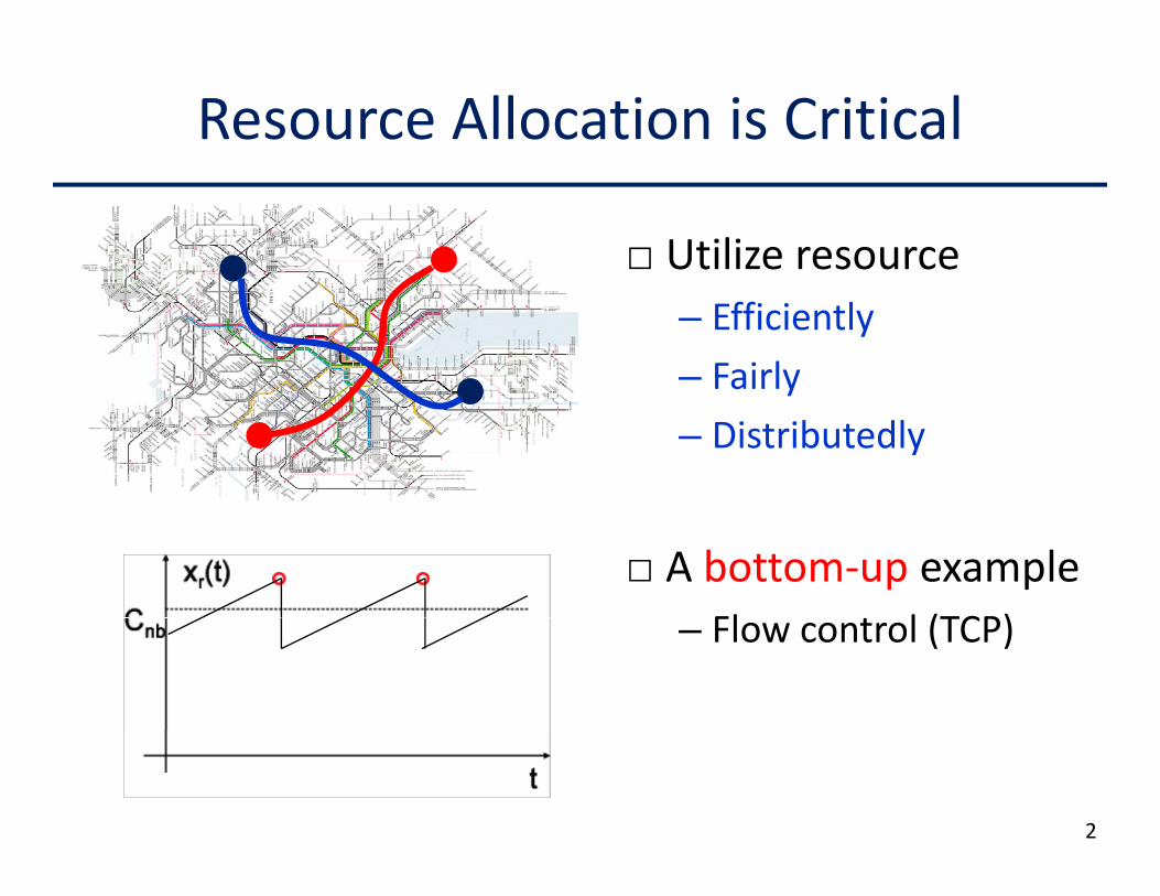
Resource Allocation is Critical

□ Utilize resource– Efficiently– Fairlyy– Distributedly

□ A bottom‐up exampleFl l (TCP)– Flow control (TCP)

2

Convex Network Optimization: Popular and EffectivePopular and Effective

□ Formulate resource allocation as a utility bl [ ll l ]maximization problem [Kelly 98, Low et. al. 99, …]X

maxx≥0

Xs∈S

Us(xs)

A Cs.t. Ax ≤ C

□ Design distributed solutionsLocal decision adapt to dynamics– Local decision, adapt to dynamics

3

Example: Understanding TCP

X 1accessing efficiency + fairness 

[Mo‐Walrand 00]max

xr≥0,r∈R−Xr∈R T

2r xr

s tX

x ≤ C ∀l ∈ Lincoming rate less 

[ ]

s.t.Xs:l∈s

xs ≤ Cl, ∀l ∈ L than the link capacity

– End users: run TCP based on end‐to‐end measurement– Routers: drop packets based on local information

□ Local actions jointly solve global problem

4

Combinatorial Network Optimization: Popular but HardPopular but Hard

□ Joint routing and flow control problem

maxx≥0,A

Xs∈S

Us(xs)s∈S

s.t. Ax ≤ C,

A ∈ {feasible?

{

routing matrices}?

□Many others: Wireless utility maximization, 

5

channel assignment, topology control …

Observations and Messages

Convex: solved Combinatorial: open

• Top‐down approach• (mostly) convex problems

• Top‐down approach• Combinatorial problemsy p

• Theory‐guided distributed solutions

p

• ??solutions

□ This talk: Explore theory‐guided design for distributedl f b l k blsolutions for combinatorial network problems

6

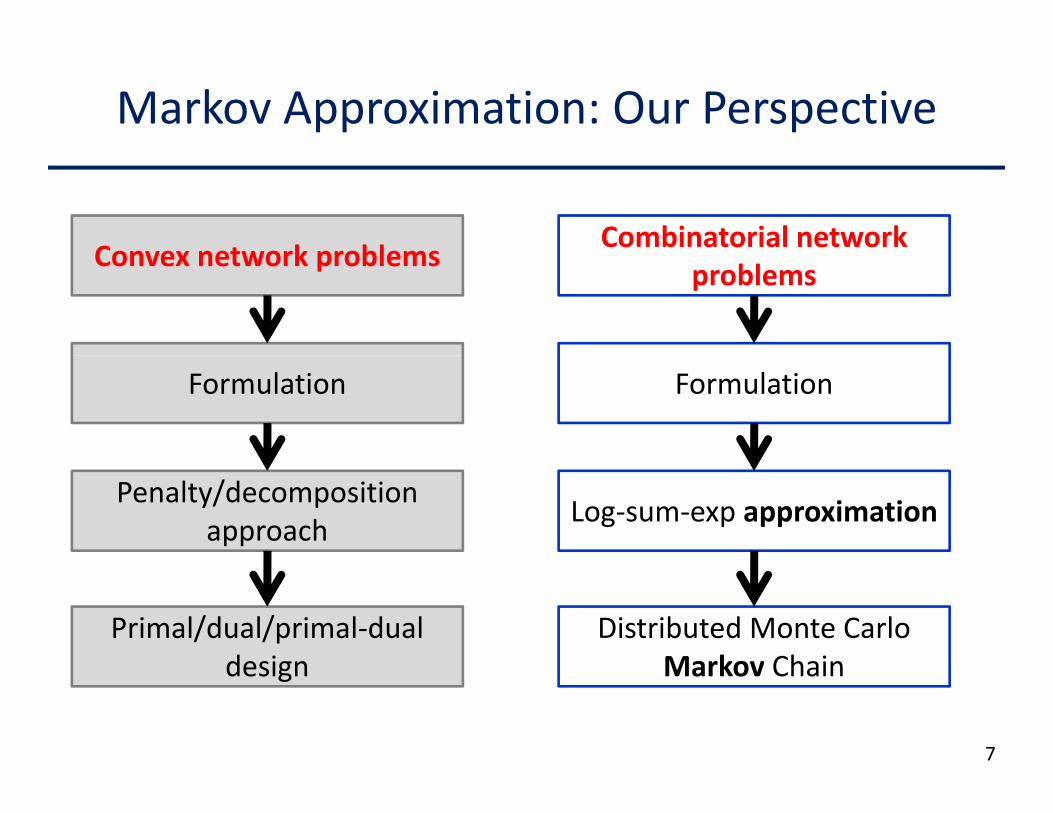
Markov Approximation: Our Perspective

Convex network problems Combinatorial network Convex network problems problems

Formulation Formulation

Penalty/decomposition approach Log‐sum‐exp approximation

Primal/dual/primal‐dual design

Distributed Monte Carlo Markov Chain

7

design Markov Chain

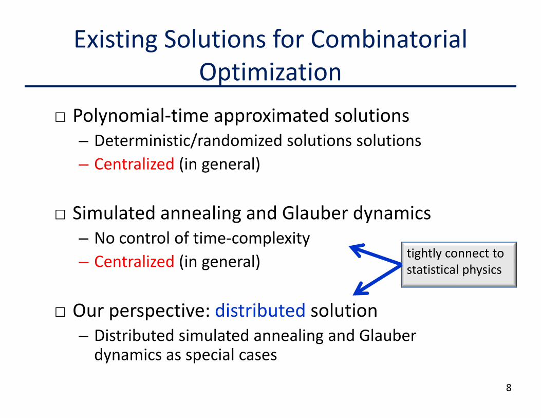
Existing Solutions for Combinatorial OptimizationOptimization

□ Polynomial‐time approximated solutions– Deterministic/randomized solutions solutions– Centralized (in general)

□ Simulated annealing and Glauber dynamicsNo control of time complexity– No control of time‐complexity

– Centralized (in general) tightly connect to statistical physics

□ Our perspective: distributed solution– Distributed simulated annealing and Glauberistributed simulated annealing and Glauberdynamics as special cases

8

Generic Form of Combinatorial Network Optimization ProblemOptimization Problem

Wmaxf∈F Wf .

□ System settings:– A set of user configurations, f =[f1, f2, …, f|R|]∈F1 2 |R|

– System performance under f, Wf

□ Goal: maximize network‐performance by choosing configurations

9

choosing configurations

Examples

□Wireless network utility maximization Newy– Configuration f: independent set

□ Channel assignments in WiFi networks

New  perspective

New

□ Channel assignments in WiFi networks– Configuration f: one combination of channel assignments

New perspective and new 

□ Path selection and flow control– Configuration f: one combination of 

solutionsselected paths □ Peering in Peer‐to‐Peer systems…

10

Wireless Network Utility Maximization

maxX

U (z )maxz≥0,p≥0

Xs∈S

Us(zs)

s.t.X

zs ≤X

pf , ∀l ∈ Ls.t.X

s:l∈s,s∈Szs ≤

Xf :l∈f

pf , ∀l ∈ LXpf = 1

□ z : rate of user s

Xf∈F

pf

Wireless link □ zs: rate of user s□ L: set of links, each with unit capacity□ F : set of all independent sets (configurations)

capacity constraints

□ pf: percentage of time f is active

11

Wireless Network Utility Maximization

maxX

Us(zs) L3∅Wireless link 

capacity constraintsz≥0,p≥0

Xs∈S

s( s)

s.t.X

zs ≤X

pf , ∀l ∈ L L2

3L1

L2

p y

Xs:l∈s,s∈S

Xf :l∈fX

pf = 1

2

L1

L2

L3

□ zs: rate of user s

f∈FL1L3

independent 3‐links interference 

graph□ L: set of links, each with unit capacity□ F : set of all independent sets (configurations)

sets

□ pf: percentage of time f is active

12

Scheduling Problem: Key Challenge

iX

U ( )X X

λ +X X

λminλ≥0

maxz≥0

Xs∈S

Us(zs)−Xs∈S

zsXl∈s

λl +maxp≥0

Xf∈F

pfXl∈f

λl

s tX

p 1 (scheduling)s.t.Xf∈F

pf = 1.

A NP h d bi i l M W i h d□ An NP‐hard combinatorial Max Weighted Independent Set problem

maxp≥0

Xf∈F

pfXl∈f

λl = maxf∈F

Xl∈f

λlX13

s.t.Xf∈F

pf = 1.

Related Work on Scheduling

□ Wireless scheduling is NP‐hard [Lin‐Shroff‐Srikant 06, …]g [ , ]

□ It is recently shown that bottom‐up CSMA can solve the scheduling problem approximately – [Wang‐Kar 05, Liew et. al. 08, Jiang‐Walrand 08, Rajagopalan‐Shah 08, Liu‐Yi‐Proutiere‐Chiang‐Poor 09, Ni‐Rajagopalan Shah 08, Liu Yi Proutiere Chiang Poor 09, NiSrikant 09, …]

f k id d i□ Our framework provides a new top‐down perspective– Note that our framework applies to general combinatorial problemsp

14

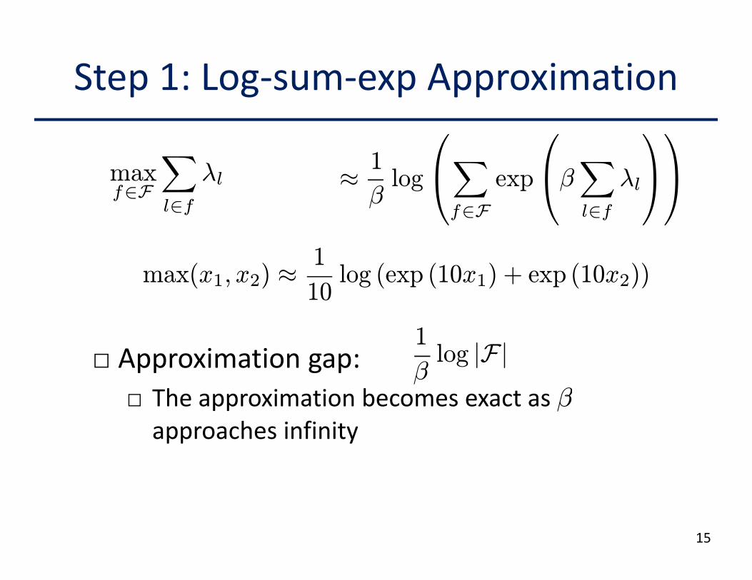
Step 1: Log‐sum‐exp Approximation

maxX

λl ≈1log

⎛⎝X exp

⎛⎝βX

λl

⎞⎠⎞⎠maxf∈F

Xl∈f

λl ≈βlog⎝X

f∈Fexp⎝β

Xl∈f

λl⎠⎠1

max(x1, x2) ≈1

10log (exp (10x1) + exp (10x2))

□ Approximation gap: □ The approximation becomes exact as β

1

βlog |F|

□ The approximation becomes exact as βapproaches infinity 

15

Step 1: Log‐sum‐exp Approximation

maxX

λl ≈1log

⎛⎝X exp

⎛⎝βX

λl

⎞⎠⎞⎠maxf∈F

Xl∈f

λl ≈βlog⎝X

f∈Fexp⎝β

Xl∈f

λl⎠⎠Log‐sum‐exp is a concave and closed function, double conjugate i i lf

maxp≥0

XpfX

λl maxp≥0

XpfX

λl −1

β

Xpf log pf

is itself 

p≥0

Xf∈F

Xl∈f

s.t.X

pf = 1.

p≥0f∈F l∈f β

f∈F

s.t.Xf∈F

pf = 1.

16

f∈F f∈F

Big Picture After Approximation

□ The new maxz≥0,p≥0

Xs∈S

Us(zs)−1

β

Xf∈F

pf log pf

primal problemf

s.t.X

s:l∈s,s∈Rzs ≤

Xf :l∈f

pf , ∀l ∈ L

□ Solution:

Xf∈F

pf = 1.

Distributed?□ Solution:⎧⎪⎪zs = αs

hU

0s(zs)−

Pl∈s λl

i+D ?

TCP‐like⎪⎪⎨⎪⎪⎪s s

hs( s)

Pl∈s l

izs

λl = kl

hPs:l∈s,s∈S zs −

Pl∈f pf (βλ)

i+λl

?Local queue

17

⎪⎩Schedule f for pf (βλ) percentage of time. ?

Schedule by a Product‐form Distribution

maxX

λl ≈1

βlog

⎛⎝X exp

⎛⎝βX

λl

⎞⎠⎞⎠maxf∈F

Xl∈f

λlβlog⎝X

f∈Fexp⎝β

Xl∈f

λl⎠⎠

pf (λ) pf (λ) =1

C(βλ)exp

⎛⎝βX

λl

⎞⎠C(βλ)

⎝l∈f

⎠

f ∈ F f ∈ F

18

□ Computed by solving the Karush‐Kuhn‐Tucker conditions to the entropy‐approximated problem

Step 2: Achieving pf(λ) Distributedly

f f 0pf (λ) =1

C(βλ)exp

⎛⎝βX

λl

⎞⎠ f fpf (λ)C(βλ)

exp⎝βXl∈f

λl⎠f 000 f 00

f ∈ F pf (λ) qf,f 0 = pf 0 (λ) qf 0,f

□ Regard pf (λ) as the steady‐state distribution of a l f ti ibl M k Ch iclass of time‐reversibleMarkov Chains– States: all the independent sets f ∈ F– Transition rate: new design spaceTransition rate: new design space– Time‐reversible: detailed balance equation holds

19

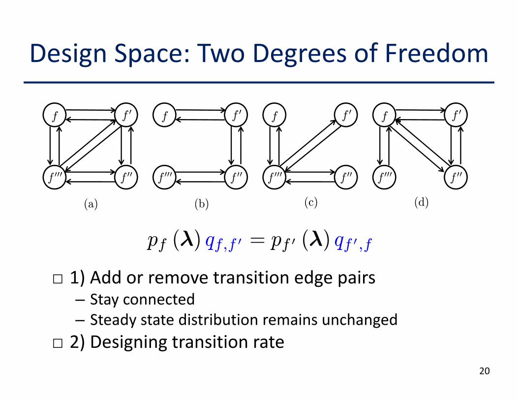
Design Space: Two Degrees of Freedom

f f 0 f f 0 f f 0 f f 0

f 000 f 00 f 000 f 00 f 000 f 00 f 000 f 00f 000 f 00

(a)

f 000 f 00

(b)

f 000 f 00

(c)

f 000 f 00

(d)

□ 1) Add or remove transition edge pairs

pf (λ) qf,f 0 = pf 0 (λ) qf 0,f

□ 1) Add or remove transition edge pairs– Stay connected– Steady state distribution remains unchangedy g

□ 2) Designing transition rate20

Design Goal: Distributed Implementation

L1Implement a Markov chain

∅L2 L1L3

Implement a Markov chain=

Realize the transitions

L3

Realize the transitions

□What leads to distributed implementation?E t iti i l l li k– Every transition involves only one link

– Transition rates Involve only local Information

21

Every Transition Involves Only One Link

□ From f to f’ = f ∪ {Li}: Li starts to send□ From f’ = f ∪ {Li} to f: Li stops transmission

L1L3

∅L2 L1L3L2 ∅∅ L1L3

LL1

LLL3 starts/stops

L1 starts/stops

22

L33‐links conflict graph

L3L3 1

Designed Markov chain

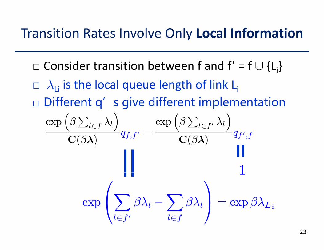
Transition Rates Involve Only Local Information

□ Consider transition between f and f’ = f ∪ {Li}□ λLi is the local queue length of link Li□ Different�q’s give�different�implementation

exp³βP

l∈f λl´

C(βλ)qf,f 0 =

exp³βP

l∈f 0 λl´

C(βλ)qf 0,f

C(βλ) C(βλ)

11

exp

⎛⎝X βλl −X

βλl

⎞⎠ = expβλL23

exp⎝Xl∈f 0

βλlXl∈f

βλl⎠ = expβλLi

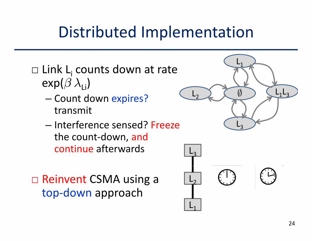
Distributed Implementation

□ Link Li counts down at rate L1

iexp(β λLi)– Count down expires? ∅L2 L1L3

transmit– Interference sensed? Freezethe count down and

L3the count‐down, and continue afterwards L3

□ Reinvent CSMA using a top‐down approach

L2top down approach

24

L1

The Overall Distributed Solution

Distributed?⎧⎪⎪⎪⎨zs = αs

hU

0s(zs)−

Pl∈s λl

i+zs

+

Distributed?TCP‐like⎨⎪⎪⎪⎩λl = kl

hPs:l∈s,s∈S zs −

Pl∈f pf (βλ)

i+λl

Distributed MCMC achieves distribution pf (βλ).

Local queue

CSMA‐like

□ Converges to the optimal solution with or

⎩f ( )

□ Converges to the optimal solution with or without time‐scale separation– Proof utilizes Lyapunov arguments, stochastic y p g ,approximation, and mixing time bounds

25

Examples

□Wireless network utility maximization Newy– Configuration f: independent set

□ Channel assignments in WiFi networks

New  perspective

New

□ Channel assignments in WiFi networks– Configuration f: one combination of channel assignments

New perspective and new 

□ Path selection and flow control– Configuration f: one combination of 

solutionsselected paths □ Peering in Peer‐to‐Peer systems…

26

Channel Assignment in WiFi Networks

– 3 WiFi channels available– N access points: each chooses one channel– Channel‐configuration affects Interference

G l i h l di t ib t dl f d f□ Goal: assign channels distributedly for good performance

27

Challenges That Make the Problem Open

□ The number of configurations are exponential□ The number of configurations are exponential – Example: 8 APs, 3 channels, 38 = 6561

□ Assignment needs to consider traffic demand

28

Problem Formulation

N

maxf∈FXi=1

Ui

³Rfi

´

□ Channel configuration f =[f1, f2, …, fN] f th h l d b AP i□ fi: the channel used by AP i

□ : downlink throughput observed by AP I d fi i f

Rfi

under configuration f□ Ui (): utility function to guarantee fairness 

29

Markov Approximation

aX NX

U³Rf´ 1 X

logmaxp≥0Xf∈F

pfXi=1

Ui

³Rfi

´−

β

Xf∈F

pf log pf

s tX

p 1

P d f l i

s.t.Xf∈F

pf = 1.

□ Product form solution:³βPN

U³Rf´´

p∗f =exp

³βPN

i=1 Ui

³Rfi

´´C

, ∀f ∈ F .

30

Distributed Markov Chain Design

□ Only allow transitions involve one AP chaning its h lchannel

□ One transition rate design:

exp³βPN

i=1 Ui

³Rfi

´´C

qf,f 0 =exp

³βPN

i=1 Ui

³Rf

0

i

´´C

qf 0,fC C

exp

Ã−β

NXUi

³Rf´! Ã

βNXU³Rf

0´!□ Recent general results: can use local estimate to 

exp

Ã−β

Xi=1

Ui

³Ri

´!exp

ÃβXi=1

Ui

³Rfi

´!

replace the global information

31

Distributed Markov Chain Implementation

□ Initially each AP randomly picks a channel

□ Each AP counts down with an exponential random variable with meanvariable with mean

exp

Ãβ

NXi=1

Ui

³Rfi

´!– Our recent general results: robust to using local estimate to replace the global information

Ãi 1

!

□ Count‐down expires– Randomly hop to a different channel– Reinitiate another count‐down

32

Simulation Results

□ Eight APs random networks (10 instances)□ Eight APs, random networks (10 instances)– 3 channels available– Each AP on average has 3 neighbors– ∆ T: aggregate throughput gap– ∆ U: aggregate utility gap– β: 10– β: 10

33

Conclusions and Future WorkCombinatorial network 

optimization Combinatorial network bl

• Top‐down approach• Combinatorial problems

problems

Formulationp

•Markov approximation for designing distribution

Formulation

Log‐sum‐expfor designing distribution solutions 

Log sum exp approximation

Distributed Monte Carlo Markov Chain

34

Conclusions and Future Work□ Convergence (mixing) time, and applications

– Connections to statistical physics (Glauber dynamics, etc.)Connections to statistical physics (Glauber dynamics, etc.)

□ Alternative Markov chain designsAlt ti t d i– Alternative parameters design

– How about non‐time‐reversible Markov chain

□ Alternative approximation?– May lead to a different set of design framework

□ Applications– Multipath/P2P routing [another example in INFOCOM 10 

]paper]– P2P VoD topology control [submitted]

35

Th kTh kThank Thank youyou

36Minghua Chen :: http://www.ie.cuhk.edu.hk/~mhchen/