markov chain monte carlo - faculty.mccombs.utexas.edu
TRANSCRIPT
Markov chain Monte Carlo1
I Historical background
I Gibbs sampler
I Metropolis-Hastings algorithms
1Based on Gamerman and Lopes (2007) Markov Chain Monte Carlo:Stochastic Simulation for Bayesian Inference, Chapman&Hall/CRC.Page 1 of 32
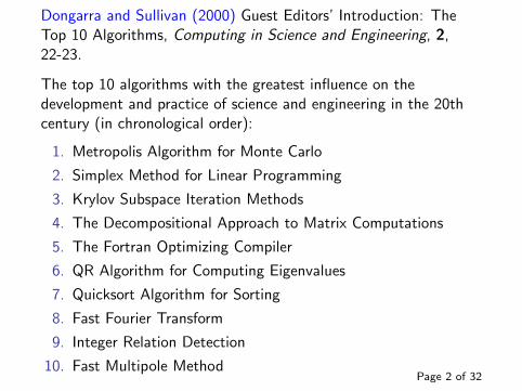
Dongarra and Sullivan (2000) Guest Editors’ Introduction: TheTop 10 Algorithms, Computing in Science and Engineering, 2,22-23.
The top 10 algorithms with the greatest influence on thedevelopment and practice of science and engineering in the 20thcentury (in chronological order):
1. Metropolis Algorithm for Monte Carlo
2. Simplex Method for Linear Programming
3. Krylov Subspace Iteration Methods
4. The Decompositional Approach to Matrix Computations
5. The Fortran Optimizing Compiler
6. QR Algorithm for Computing Eigenvalues
7. Quicksort Algorithm for Sorting
8. Fast Fourier Transform
9. Integer Relation Detection
10. Fast Multipole MethodPage 2 of 32
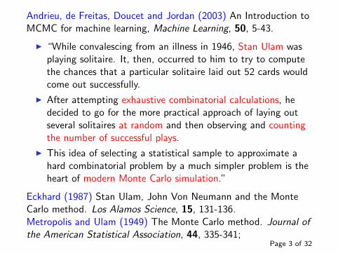
Andrieu, de Freitas, Doucet and Jordan (2003) An Introduction toMCMC for machine learning, Machine Learning, 50, 5-43.
I “While convalescing from an illness in 1946, Stan Ulam wasplaying solitaire. It, then, occurred to him to try to computethe chances that a particular solitaire laid out 52 cards wouldcome out successfully.
I After attempting exhaustive combinatorial calculations, hedecided to go for the more practical approach of laying outseveral solitaires at random and then observing and countingthe number of successful plays.
I This idea of selecting a statistical sample to approximate ahard combinatorial problem by a much simpler problem is theheart of modern Monte Carlo simulation.”
Eckhard (1987) Stan Ulam, John Von Neumann and the MonteCarlo method. Los Alamos Science, 15, 131-136.Metropolis and Ulam (1949) The Monte Carlo method. Journal ofthe American Statistical Association, 44, 335-341;
Page 3 of 32

1940s and 1950s
Stan Ulam soon realized that computers could be used in thisfashion to answer questions of neutron diffusion and mathematicalphysics;
He contacted John Von Neumann and they developed many MonteCarlo algorithms (importance sampling, rejection sampling, etc);
In the 1940s Nick Metropolis and Klari Von Neumann designednew controls for the state-of-the-art computer (ENIAC);
Metropolis and Ulam (1949) The Monte Carlo method. Journal ofthe American Statistical Association, 44, 335-341;
Metropolis, Rosenbluth, Rosenbluth, Teller and Teller (1953)Equations of state calculations by fast computing machines.Journal of Chemical Physics, 21, 1087-1091.
Page 4 of 32
1970s
Hastings and his student Peskun showed that Metropolis and themore general Metropolis-Hastings algorithm are particularinstances of a larger family of algorithms.
Hastings (1970) Monte Carlo sampling methods using Markovchains and their applications. Biometrika, 57, 97-109.
Peskun (1973) Optimum Monte-Carlo sampling using Markovchains. Biometrika, 60, 607-612.
Page 5 of 32
1980s
Geman and Geman (1984)Stochastic relaxation, Gibbs distributions and the Bayesianrestoration of images. IEEE Transactions on Pattern Analysis andMachine Intelligence, 6, 721-741.
Pearl (1987)Evidential reasoning using stochastic simulation. ArtificialIntelligence, 32, 245-257.
Page 6 of 32
1990s
Tanner and Wong (1987)The calculation of posterior distributions by data augmentation.Journal of the American Statistical Association, 82, 528-550.
Gelfand and Smith (1990)Sampling-based approaches to calculating marginal densities.Journal of the American Statistical Association, 85, 398-409.
Page 7 of 32
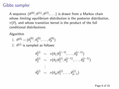
Gibbs sampler
A sequence {θ(0), θ(1), θ(2), . . . } is drawn from a Markov chainwhose limiting equilibrium distribution is the posterior distribution,π(θ), and whose transition kernel is the product of the fullconditional distributions:
Algorithm
1. θ(0) = (θ(0)1 , θ
(0)2 , . . . , θ
(0)p )
2. θ(j) is sampled as follows:
θ(j)1 ∼ π(θ1|θ(j−1)
2 , . . . , θ(j−1)p )
θ(j)2 ∼ π(θ2|θ(j)
1 , θ(j−1)3 , . . . , θ
(j−1)p )
...
θ(j)p ∼ π(θp|θ(j)
1 , . . . , θ(j)p−1)
Page 8 of 32
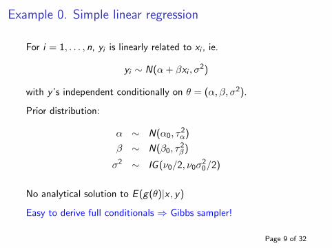
Example 0. Simple linear regression
For i = 1, . . . , n, yi is linearly related to xi , ie.
yi ∼ N(α + βxi , σ2)
with y ’s independent conditionally on θ = (α, β, σ2).
Prior distribution:
α ∼ N(α0, τ2α)
β ∼ N(β0, τ2β)
σ2 ∼ IG (ν0/2, ν0σ20/2)
No analytical solution to E (g(θ)|x , y)
Easy to derive full conditionals ⇒ Gibbs sampler!
Page 9 of 32
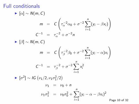
Full conditionalsI [α] ∼ N(m,C )
m = C
(τ−2α α0 + σ−2
n∑
i=1
(yi − βxi )
)
C−1 = τ−2α + σ−2n
I [β] ∼ N(m,C )
m = C
(τ−2β β0 + σ−2
n∑
i=1
(yi − α)xi
)
C−1 = τ−2β + σ−2
n∑
i=1
x2i
I [σ2] ∼ IG(ν1/2, ν1σ
21/2
)
ν1 = ν0 + n
ν1σ21 = ν0σ
20 +
n∑
i=1
(yi − α− βxi )2
Page 10 of 32
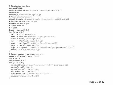
# Simulating the data
set.seed(1244)
n=100;alpha=0;beta=2;sig2=0.5;true=c(alpha,beta,sig2)
x=rnorm(n)
y=rnorm(n,alpha+beta*x,sqrt(sig2))
# Prior hyperparameters
alpha0=0;tau2a=10;beta0=0;tau2b=10;nu0=3;s02=1;nu0s02=nu0*s02
# Setting up starting values
alpha=0;beta=0;sig2=1
# Gibbs sampler
M = 1000
draws = matrix(0,M,3)
for (i in 1:M){
var = 1/(1/tau2a+n/sig2)
mean = var*(sum(y-beta*x)/sig2+alpha0/tau2a)
alpha = rnorm(1,mean,sqrt(var))
var = 1/(1/tau2b+sum(x^2)/sig2)
mean = var*(sum((y-alpha)*x)/sig2+beta0/tau2b)
beta = rnorm(1,mean,sqrt(var))
sig2 = 1/rgamma(1,(nu0+n)/2,(nu0s02+sum((y-alpha-beta*x)^2)/2))
draws[i,] = c(alpha,beta,sig2)
}
# Markov chains + marginal posterior
names = c("alpha","beta","sig2")
ind = 101:M
par(mfrow=c(3,3))
for (i in 1:3){
ts.plot(draws[,i],xlab="iterations",ylab="",main=names[i])
abline(v=ind[1],col=4)
abline(h=true[i],col=2,lwd=2)
acf(draws[ind,i],main="")
hist(draws[ind,i],prob=T,main="",xlab="")
abline(v=true[i],col=2,lwd=2)
}
Page 11 of 32
alpha
iterations
0 200 400 600 800 1000
−0.
3−
0.1
0.1
0.2
0 5 10 15 20 25 30
0.0
0.2
0.4
0.6
0.8
1.0
Lag
AC
F
Den
sity
−0.3 −0.1 0.0 0.1 0.2
01
23
45
beta
iterations
0 200 400 600 800 1000
1.8
1.9
2.0
2.1
2.2
2.3
0 5 10 15 20 25 30
0.0
0.2
0.4
0.6
0.8
1.0
Lag
AC
F
Den
sity
1.8 1.9 2.0 2.1 2.2 2.3
01
23
4
sig2
iterations
0 200 400 600 800 1000
0.4
0.5
0.6
0.7
0.8
0 5 10 15 20 25 30
0.0
0.2
0.4
0.6
0.8
1.0
Lag
AC
F
Den
sity
0.4 0.5 0.6 0.7 0.8 0.9
01
23
45
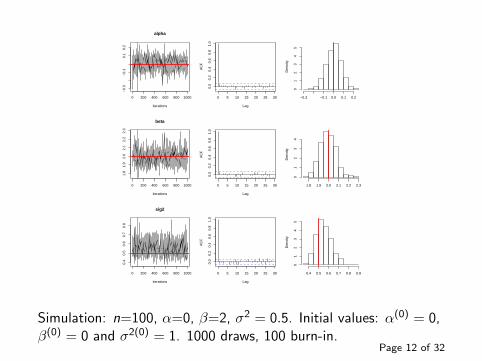
Simulation: n=100, α=0, β=2, σ2 = 0.5. Initial values: α(0) = 0,β(0) = 0 and σ2(0) = 1. 1000 draws, 100 burn-in.
Page 12 of 32
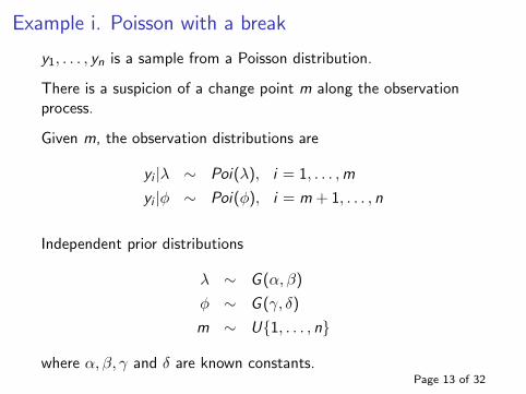
Example i. Poisson with a break
y1, . . . , yn is a sample from a Poisson distribution.
There is a suspicion of a change point m along the observationprocess.
Given m, the observation distributions are
yi |λ ∼ Poi(λ), i = 1, . . . ,m
yi |φ ∼ Poi(φ), i = m + 1, . . . , n
Independent prior distributions
λ ∼ G (α, β)
φ ∼ G (γ, δ)
m ∼ U{1, . . . , n}
where α, β, γ and δ are known constants.Page 13 of 32
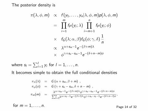
The posterior density is
π(λ, φ, m) ∝ f (y1, . . . , yn|λ, φ,m)p(λ, φ,m)
=m∏
i=1
fP(yi ; λ)n∏
i=m+1
fP(yi ; φ)
× fG (λ;α, β)fG (φ; γ, δ)1
n
∝ λα+sm−1e−(β+m)λ
× φγ+sn−sm−1e−(δ+n−m)φ
where sl =∑l
i=1 yi for l = 1, . . . , n.
It becomes simple to obtain the full conditional densities
πλ(λ) = G (α + sm, β + m) ,
πφ(φ) = G (γ + sn − sm, δ + n −m) ,
πm(m) =λα+sm−1e−(β+m)λφγ+sn−sm−1e−(δ+n−m)φ
Pnl=1λ
α+sl−1e−(β+l)λφγ+sn−sl−1e−(δ+n−l)φ,
for m = 1, . . . , n. Page 14 of 32
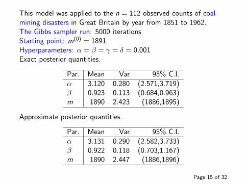
This model was applied to the n = 112 observed counts of coalmining disasters in Great Britain by year from 1851 to 1962.The Gibbs sampler run: 5000 iterationsStarting point: m(0) = 1891Hyperparameters: α = β = γ = δ = 0.001Exact posterior quantities.
Par. Mean Var 95% C.I.
α 3.120 0.280 (2.571,3.719)β 0.923 0.113 (0.684,0.963)m 1890 2.423 (1886,1895)
Approximate posterior quantities.
Par. Mean Var 95% C.I.
α 3.131 0.290 (2.582,3.733)β 0.922 0.118 (0.703,1.167)m 1890 2.447 (1886,1896)
Page 15 of 32
(a)
years
1860 1880 1900 1920 1940 19600
12
34
56
(b)
years
1860 1880 1900 1920 1940 1960
050
100
150
(c)
1 2 3 4
0.0
0.5
1.0
1.5 π(φ)
π(λ)
(d)
years
1880 1885 1890 1895 1900
0.00
0.05
0.10
0.15
0.20
0.25
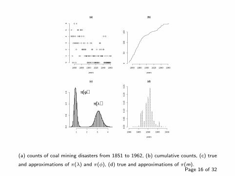
(a) counts of coal mining disasters from 1851 to 1962, (b) cumulative counts, (c) true
and approximations of π(λ) and π(φ), (d) true and approximations of π(m).Page 16 of 32
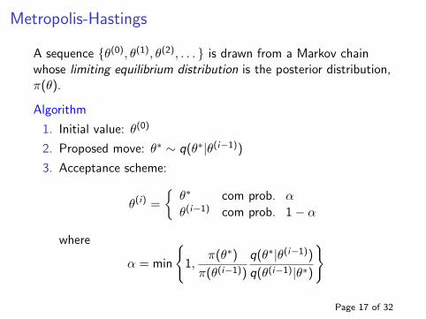
Metropolis-Hastings
A sequence {θ(0), θ(1), θ(2), . . . } is drawn from a Markov chainwhose limiting equilibrium distribution is the posterior distribution,π(θ).
Algorithm
1. Initial value: θ(0)
2. Proposed move: θ∗ ∼ q(θ∗|θ(i−1))
3. Acceptance scheme:
θ(i) =
{θ∗ com prob. α
θ(i−1) com prob. 1− α
where
α = min
{1,
π(θ∗)π(θ(i−1))
q(θ∗|θ(i−1))
q(θ(i−1)|θ∗)
}
Page 17 of 32
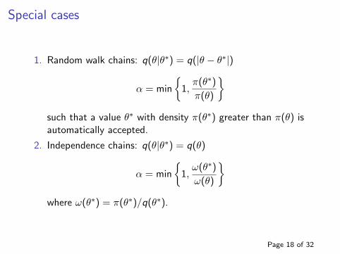
Special cases
1. Random walk chains: q(θ|θ∗) = q(|θ − θ∗|)
α = min
{1,
π(θ∗)π(θ)
}
such that a value θ∗ with density π(θ∗) greater than π(θ) isautomatically accepted.
2. Independence chains: q(θ|θ∗) = q(θ)
α = min
{1,
ω(θ∗)ω(θ)
}
where ω(θ∗) = π(θ∗)/q(θ∗).
Page 18 of 32
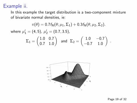
Example ii.In this example the target distribution is a two-component mixtureof bivariate normal densities, ie:
π(θ) = 0.7fN(θ; µ1, Σ1) + 0.3fN(θ;µ2,Σ2).
where µ′1 = (4, 5), µ′2 = (0.7, 3.5),
Σ1 =
(1.0 0.70.7 1.0
)and Σ2 =
(1.0 −0.7−0.7 1.0
).
−2
0
2
4
60
2
4
6
8
0.0
0.2
0.4
0.6
0.8
θ1
θ2
Page 19 of 32
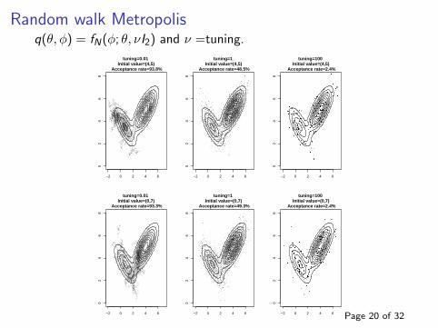
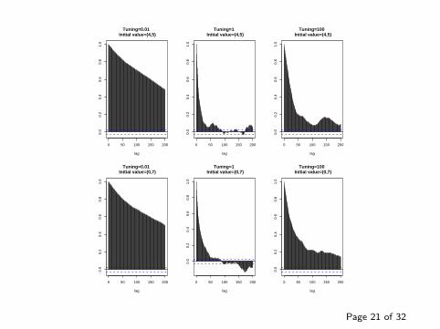
Random walk Metropolisq(θ, φ) = fN(φ; θ, νI2) and ν =tuning.
−2 0 2 4 6
02
46
8
tuning=0.01 Initial value=(4,5)
Acceptance rate=93.8%
−2 0 2 4 6
02
46
8
tuning=1 Initial value=(4,5)
Acceptance rate=48.5%
−2 0 2 4 6
02
46
8
tuning=100 Initial value=(4,5)
Acceptance rate=2.4%
−2 0 2 4 6
02
46
8
tuning=0.01 Initial value=(0,7)
Acceptance rate=93.3%
−2 0 2 4 6
02
46
8
tuning=1 Initial value=(0,7)
Acceptance rate=49.3%
−2 0 2 4 6
02
46
8
tuning=100 Initial value=(0,7)
Acceptance rate=2.4%
Page 20 of 32
0 50 100 150 200
0.0
0.2
0.4
0.6
0.8
1.0
lag
Tuning=0.01 Initial value=(4,5)
0 50 100 150 200
0.0
0.2
0.4
0.6
0.8
1.0
lag
Tuning=1 Initial value=(4,5)
0 50 100 150 200
0.0
0.2
0.4
0.6
0.8
1.0
lag
Tuning=100 Initial value=(4,5)
0 50 100 150 200
0.0
0.2
0.4
0.6
0.8
1.0
lag
Tuning=0.01 Initial value=(0,7)
0 50 100 150 200
0.0
0.2
0.4
0.6
0.8
1.0
lag
Tuning=1 Initial value=(0,7)
0 50 100 150 200
0.0
0.2
0.4
0.6
0.8
1.0
lag
Tuning=100 Initial value=(0,7)
Page 21 of 32
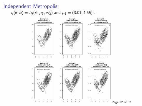
Independent Metropolisq(θ, φ) = fN(φ; µ3, νI2) and µ3 = (3.01, 4.55)′.
−2 0 2 4 6
02
46
8
tuning=0.5 Initial value=(4,5)
Acceptance rate=9.9%
Acceptance rate=9.9%
−2 0 2 4 6
02
46
8
tuning=5 Initial value=(4,5)
Acceptance rate=30.9%
Acceptance rate=30.9%
−2 0 2 4 6
02
46
8
tuning=50 Initial value=(4,5)
Acceptance rate=5%
Acceptance rate=5%
−2 0 2 4 6
02
46
8
tuning=0.5 Initial value=(0,7)
Acceptance rate=29.4%
Acceptance rate=29.4%
−2 0 2 4 6
02
46
8
tuning=5 Initial value=(0,7)
Acceptance rate=32.2%
Acceptance rate=32.2%
−2 0 2 4 6
02
46
8
tuning=50 Initial value=(0,7)
Acceptance rate=4.3%
Acceptance rate=4.3%
Page 22 of 32
0 50 100 150 200
0.0
0.2
0.4
0.6
0.8
1.0
lag
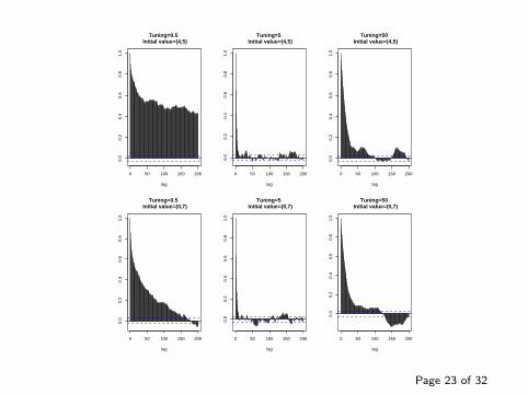
Tuning=0.5 Initial value=(4,5)
0 50 100 150 200
0.0
0.2
0.4
0.6
0.8
1.0
lag
Tuning=5 Initial value=(4,5)
0 50 100 150 200
0.0
0.2
0.4
0.6
0.8
1.0
lag
Tuning=50 Initial value=(4,5)
0 50 100 150 200
0.0
0.2
0.4
0.6
0.8
1.0
lag
Tuning=0.5 Initial value=(0,7)
0 50 100 150 200
0.0
0.2
0.4
0.6
0.8
1.0
lag
Tuning=5 Initial value=(0,7)
0 50 100 150 200
0.0
0.2
0.4
0.6
0.8
1.0
lag
Tuning=50 Initial value=(0,7)
Page 23 of 32
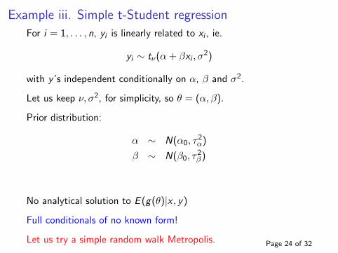
Example iii. Simple t-Student regression
For i = 1, . . . , n, yi is linearly related to xi , ie.
yi ∼ tν(α + βxi , σ2)
with y ’s independent conditionally on α, β and σ2.
Let us keep ν, σ2, for simplicity, so θ = (α, β).
Prior distribution:
α ∼ N(α0, τ2α)
β ∼ N(β0, τ2β)
No analytical solution to E (g(θ)|x , y)
Full conditionals of no known form!
Let us try a simple random walk Metropolis. Page 24 of 32
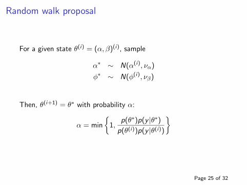
Random walk proposal
For a given state θ(i) = (α, β)(i), sample
α∗ ∼ N(α(i), να)
φ∗ ∼ N(φ(i), νβ)
Then, θ(i+1) = θ∗ with probability α:
α = min
{1,
p(θ∗)p(y |θ∗)p(θ(i))p(y |θ(i))
}
Page 25 of 32
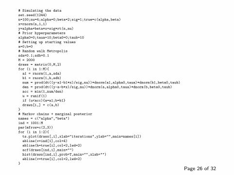
# Simulating the data
set.seed(1244)
n=100;nu=4;alpha=0;beta=2;sig=1;true=c(alpha,beta)
x=rnorm(n,1,1)
y=alpha+beta*x+sig*rt(n,nu)
# Prior hyperparameters
alpha0=0;taua=10;beta0=0;taub=10
# Setting up starting values
a=0;b=0
# Random walk Metropolis
sda=0.1;sdb=0.1
M = 2000
draws = matrix(0,M,2)
for (i in 1:M){
a1 = rnorm(1,a,sda)
b1 = rnorm(1,b,sdb)
num = prod(dt((y-a1-b1*x)/sig,nu))*dnorm(a1,alpha0,taua)*dnorm(b1,beta0,taub)
den = prod(dt((y-a-b*x)/sig,nu))*dnorm(a,alpha0,taua)*dnorm(b,beta0,taub)
acc = min(1,num/den)
u = runif(1)
if (u<acc){a=a1;b=b1}
draws[i,] = c(a,b)
}
# Markov chains + marginal posterior
names = c("alpha","beta")
ind = 1001:M
par(mfrow=c(2,3))
for (i in 1:2){
ts.plot(draws[,i],xlab="iterations",ylab="",main=names[i])
abline(v=ind[1],col=4)
abline(h=true[i],col=2,lwd=2)
acf(draws[ind,i],main="")
hist(draws[ind,i],prob=T,main="",xlab="")
abline(v=true[i],col=2,lwd=2)
}
Page 26 of 32
alpha
iterations
0 500 1000 1500 2000
−0.
6−
0.2
0.0
0.2
0.4
0.6
0 5 10 15 20 25 30
0.0
0.2
0.4
0.6
0.8
1.0
Lag
AC
F
Den
sity
−0.4 −0.2 0.0 0.2 0.4
0.0
0.5
1.0
1.5
2.0
2.5
beta
iterations
0 500 1000 1500 2000
0.0
0.5
1.0
1.5
2.0
2.5
0 5 10 15 20 25 30
0.0
0.2
0.4
0.6
0.8
1.0
Lag
AC
F
Den
sity
1.6 1.8 2.0 2.2
0.0
0.5
1.0
1.5
2.0
2.5
3.0
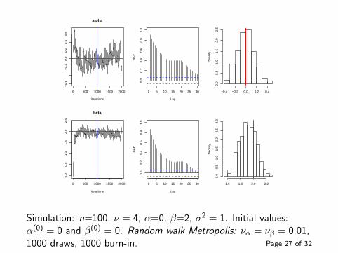
Simulation: n=100, ν = 4, α=0, β=2, σ2 = 1. Initial values:α(0) = 0 and β(0) = 0. Random walk Metropolis: να = νβ = 0.01,1000 draws, 1000 burn-in. Page 27 of 32
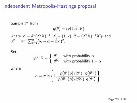
Independent Metropolis-Hastings proposal
Sample θ∗ fromq(θ) = fN(θ, θ̂, V )
where V = σ̂2(X ′X )−1, X = (1, x), θ̂ = (X ′X )−1X ′y andσ̂2 = n−1
∑ni=1(yi − α̂− β̂xi )
2.
Set
θ(i+1) =
{θ∗ with probability α
θ(i) with probability 1− α
where
α = min
{1,
p(θ∗)p(y |θ∗)p(θ(i))p(y |θ(i))
q(θ(i))
q(θ∗)
}.
Page 28 of 32
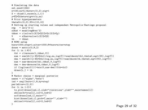
# Simulating the data
set.seed(1244)
n=100;nu=4;theta=c(0,2);sig=1
X = cbind(1,rnorm(n,1,1))
y=X%*%theta+sig*rt(n,nu)
# Prior hyperparameters
theta0=c(0,0);V0=c(10,10)
# Setting up starting values and independent Metropolis-Hastings proposal
reg = lm(y~X-1)
s2hat = mean(reg$res^2)
thhat = c(solve(t(X)%*%X)%*%t(X)%*%y)
V = s2hat*solve(t(X)%*%X)
th = thhat
# MCMC setup
burn=1000;step=1;niter=1000;M=burn+niter*step
draws = matrix(0,M,2)
for (i in 1:M){
th1 = c(rmvnorm(1,thhat,V))
num = sum(dt((y-X%*%th1)/sig,nu,log=T))+sum(dnorm(th1,theta0,sqrt(V0),log=T))
den = sum(dt((y-X%*%th)/sig,nu,log=T))+sum(dnorm(th,theta0,sqrt(V0),log=T))
num = num-dmvnorm(th1,thhat,V,log=T)
den = den-dmvnorm(th,thhat,V,log=T)
if (log(runif(1))<min(0,num-den)){th=th1}
draws[i,] = th
}
# Markov chains + marginal posterior
names = c("alpha","beta")
ind = seq((burn+1),M,by=step)
par(mfrow=c(2,3))
for (i in 1:2){
ts.plot(draws[ind,i],xlab="iterations",ylab="",main=names[i])
abline(h=true[i],col=2,lwd=2)
acf(draws[ind,i],main="")
hist(draws[ind,i],prob=T,main="",xlab="")
abline(v=true[i],col=2,lwd=2)
}Page 29 of 32
alpha
iterations
0 200 400 600 800 1000
−0.
4−
0.2
0.0
0.2
0.4
0.6
0 5 10 15 20 25 30
0.0
0.2
0.4
0.6
0.8
1.0
Lag
AC
F
Den
sity
−0.4 0.0 0.2 0.4 0.6
0.0
0.5
1.0
1.5
2.0
beta
iterations
0 200 400 600 800 1000
1.6
1.8
2.0
2.2
2.4
0 5 10 15 20 25 30
0.0
0.2
0.4
0.6
0.8
1.0
Lag
AC
F
Den
sity
1.6 1.8 2.0 2.2 2.4
0.0
0.5
1.0
1.5
2.0
2.5
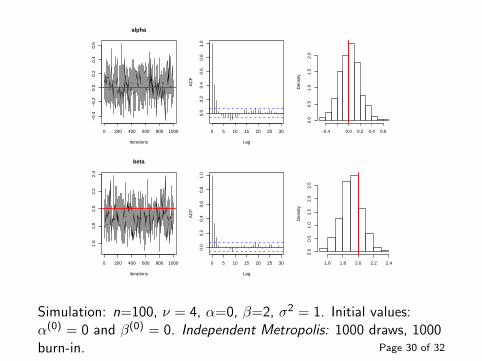
Simulation: n=100, ν = 4, α=0, β=2, σ2 = 1. Initial values:α(0) = 0 and β(0) = 0. Independent Metropolis: 1000 draws, 1000burn-in. Page 30 of 32
References
Andrieu, de Freitas, Doucet and Jordan (2003) An Introduction to MCMC for machinelearning, Machine Learning, 50, 5-43.
Dongarra and Sullivan (2000) Guest Editors’ Introduction: The Top 10 Algorithms,Computing in Science and Engineering, 2, 22-23.
Eckhard (1987) Stan Ulam, John Von Neumann and the Monte Carlo method. LosAlamos Science, 15, 131-136.
Gelfand, A. E. and Smith, A. F. M. (1990) Sampling-based approaches to calculatingmarginal densities. Journal of the American Statistical Association, 85, 398-409.
Geman and Geman (1984) Stochastic relaxation, Gibbs distributions and the Bayesianrestoration of images. IEEE Transactions on Pattern Analysis and MachineIntelligence, 6, 721-741.
Hastings (1970) Monte Carlo sampling methods using Markov chains and theirapplications. Biometrika, 57, 97-109.
Metropolis, N., Rosenbluth, A. W., Rosenbluth, M. N., Teller, A. H. and Teller, E.(1953) Equation of state calculations by fast computing machine. Journal of ChemicalPhysics, 21, 1087-91.
Page 31 of 32
Metropolis and Ulam (1949) The Monte Carlo method. Journal of the AmericanStatistical Association, 44, 335-341.
Pearl (1987) Evidential reasoning using stochastic simulation. Artificial Intelligence,32, 245-257.
Peskun (1973) Optimum Monte-Carlo sampling using Markov chains. Biometrika, 60,607-612.
Tanner and Wong (1987) The calculation of posterior distributions by dataaugmentation. Journal of the American Statistical Association, 82, 528-550.
Page 32 of 32