markov chain monte carlo estimation of stochastic ... · markov chain monte carlo estimation of...
TRANSCRIPT

Tampere University of Technology
Markov Chain Monte Carlo Estimation of Stochastic Volatility Models with Finite andInfinite Activity Lévy Jumps
CitationYang, H. (2015). Markov Chain Monte Carlo Estimation of Stochastic Volatility Models with Finite and InfiniteActivity Lévy Jumps: Evidence for Efficient Models and Algorithms. (Tampere University of Technology.Publication; Vol. 1331). Tampere University of Technology.Year2015
VersionPublisher's PDF (version of record)
Link to publicationTUTCRIS Portal (http://www.tut.fi/tutcris)
Take down policyIf you believe that this document breaches copyright, please contact [email protected], and we will remove accessto the work immediately and investigate your claim.
Download date:05.04.2020


Tampereen teknillinen yliopisto. Julkaisu 1331 Tampere University of Technology. Publication 1331 Hanxue Yang Markov Chain Monte Carlo Estimation of Stochastic Volatility Models with Finite and Infinite Activity Lévy Jumps Evidence for Efficient Models and Algorithms Thesis for the degree of Doctor of Philosophy degree to be presented with due permission for public examination and criticism in Festia Building, Auditorium Pieni Sali 1, at Tampere University of Technology, on the 13th of November 2015, at 12 noon. Tampereen teknillinen yliopisto - Tampere University of Technology Tampere 2015

ISBN 978-952-15-3597-0 (printed) ISBN 978-952-15-3617-5 (PDF) ISSN 1459-2045

Abstract
A financial model plays a key role in the valuation and risk management of financialderivatives, and it serves as an important tool for investors to measure the risk exposure oftheir portfolios and make predictions and decisions. However, the popular a�ne stochasticvolatility models without jumps, such as the Heston model, have been questioned in thefinance literature in terms of their appropriateness for modelling stock prices and pricingderivatives. Many alternative model specifications have been proposed in recent decades,including the specification of non-a�ne variance dynamics and the inclusion of Lévyjumps. However, the complexity introduced by further model specifications leads to poorprobabilistic properties, and hence most popular estimation methods are not applicable.The Bayesian estimation method is among the few that work. In this thesis, I discuss therole of new model specifications and investigate the performance of Bayesian estimationmethods.
First, I use an extensive empirical data set to study how the use of infinite-activity Lévyjumps in stock returns and variance improves model performance. The stock returns andvariance are driven by di�usions and di�erent Lévy jumps, including the finite-activitycompound Poisson jump and infinite-activity Variance Gamma and Normal InverseGaussian (NIG) jumps. Moreover, the non-a�ne linear variance process is compared tothe a�ne square-root stochastic process. With the conventional Markov Chain MonteCarlo (MCMC) algorithms, including the Gibbs sampler and Metropolis-Hastings (MH)methods, and the Damien-Wakefield-Walker method to cope with complicated posteriors,eighteen di�erent model specifications are estimated using the joint information of theS&P 500 index and the VIX index for 1996–2009. There is clear evidence that in terms ofthe goodness of fit and option pricing performance, a relatively parsimonious model withinfinite-activity NIG jumps in returns and non-a�ne variance dynamics is particularlycompetitive.
In the second part of the thesis, I examine the performance of advanced MCMC algorithms.The e�ciency of the MH algorithm has been questioned because of its slow mixing speed,especially in the presence of high dimensions and a strong dependence between modelparameters and state variables. Generally, a class of algorithms seeks to improve theMH by constructing more e�ective proposals, and another combines the MCMC withthe Sequential Monte Carlo algorithms. To investigate, I first conduct simulation studiesto compare the estimation performance of seven advanced Bayesian estimation methodsagainst the MH. Specifically, I use the a�ne Heston model, the a�ne Bates model, and ana�ne model with NIG return jumps, and examine whether the di�erent jump structuresa�ect the estimation results. Second, I estimate the non-a�ne model with NIG returnjumps using the joint information of the S&P 500 index and the VIX for 2002–2005with selected algorithms that perform well in the simulation studies. The results of thesimulation and empirical studies are mixed about the performance of the algorithms. The
i

ii Abstract
Fast Universal Self-tuned Sampler algorithms are particularly competitive in generatingvirtually independent samples and achieving the fastest mixing with a fixed numberof MCMC runs, and their performance is stable regardless of the model specifications.However, they are computationally expensive. The computational costs of the ParticleMarkov Chain Monte Carlo (PMCMC) methods are much cheaper and also e�cient inmixing, and they perform best when estimating the models without jumps/with NIGjumps in the simulation studies, as well as in the fit to the VIX in the empirical studies.However, the PMCMC methods are more vulnerable to model specifications than theother algorithms; in particular, the rare large compound Poisson jumps in the Batesmodel significantly reduce the acceptance rate and worsen the estimation performance ofthe PMCMC methods.

Preface
The research presented in this thesis was carried out at the Department of IndustrialManagement at Tampere University of Technology between 2013 and 2015, within theMarie Curie Initial Training Network HPCFinance. During the writing of this thesis, Iwas financially supported by the European Union Seventh Framework Programme undergrant agreement No. 289032.
I would like to express my sincere gratitude to my supervisor, Professor Juho Kanniainen,for giving me such an invaluable opportunity to work on the HPCFinance project, andmore importantly, for his insightful guidance and consistent support that helped memanage many di�cult problems. In my research, I have always been encouraged byhis enthusiasm and honest criticism and advice. I am also especially grateful for theinspiring cooperation with, and support from, Professor Luca Martino, who proposed anddeveloped the powerful FUSS algorithms and guided me in applying the algorithms tofinancial problems. In addition, I would like to express my gratitude to the pre-examiners,Professor Michael Johannes and Professor Andreas Kaeck, for their helpful commentsand suggestions.
Furthermore, I wish to thank my colleagues at the Department of Industrial Managementand in the HPCFinance project. In particular, I thank Milla Siikanen, Sindhuja Ran-ganathan, Jaakko Valli, and Binghuan Lin in the finance group for the helpful discussionsand activities outside of work. Special thanks go to my o�cemates, Jun Hu and Ye Yue,for providing a fun and stimulating work environment. I am also thankful to the projectmanagers, Dr. Santiago Velasquez and Dr. Hanna-Riikka Sundberg, and the departmentsecretary, Ms. Heli Kiviranta, for their assistance and administrative support.
I want to thank Jukka Annala and his wife Tuija for inviting me to their beautifulhome and summer cottage. I will never forget the journey into the deep forest and theexperiences of taking a sauna and jumping into the cold lake, picking mushrooms, andtasting karjalanpiirakka. A special mention goes to the lovely couple Huiling Wangand Tinghuai Wang. I am glad to have friends like you, who have made my life hereunforgettable.
Last but not least, I owe my deepest thanks to my parents and my dearest grandmotherfor their endless encouragement and love. Thank you for sharing your lives with me. Youremain my best friends, no matter how far away you are.
iii


Contents
Abstract i
Preface iii
Acronyms vii
1 Introduction 11.1 Background and Motivation . . . . . . . . . . . . . . . . . . . . . . . . . . 11.2 Questions and Research Methods . . . . . . . . . . . . . . . . . . . . . . . 61.3 Outline and Contributions of the Thesis . . . . . . . . . . . . . . . . . . . 8
2 Jumps and Volatility Dynamics for the S&P 500 Index:Conventional MCMC 132.1 Description of Models and Notations . . . . . . . . . . . . . . . . . . . . . 132.2 Change of Measure . . . . . . . . . . . . . . . . . . . . . . . . . . . . . . . 162.3 VIX . . . . . . . . . . . . . . . . . . . . . . . . . . . . . . . . . . . . . . . 192.4 Estimation Method . . . . . . . . . . . . . . . . . . . . . . . . . . . . . . . 212.5 Data Description and Option Pricing Settings . . . . . . . . . . . . . . . . 252.6 Estimation Results . . . . . . . . . . . . . . . . . . . . . . . . . . . . . . . 282.7 Discussion . . . . . . . . . . . . . . . . . . . . . . . . . . . . . . . . . . . . 45
3 Model Estimation with Advanced MCMC Algorithms:Simulation Studies 473.1 Motivation . . . . . . . . . . . . . . . . . . . . . . . . . . . . . . . . . . . 473.2 Review: Conventional MCMC Methods . . . . . . . . . . . . . . . . . . . 483.3 Particle Filters . . . . . . . . . . . . . . . . . . . . . . . . . . . . . . . . . 503.4 Advanced MCMC Methods . . . . . . . . . . . . . . . . . . . . . . . . . . 513.5 Simulation Studies: Data Generation . . . . . . . . . . . . . . . . . . . . . 563.6 Implementation of Algorithms . . . . . . . . . . . . . . . . . . . . . . . . . 583.7 Results . . . . . . . . . . . . . . . . . . . . . . . . . . . . . . . . . . . . . . 623.8 Discussion . . . . . . . . . . . . . . . . . . . . . . . . . . . . . . . . . . . . 76
4 Model Estimation with Advanced MCMC Algorithms:Empirical Studies 794.1 Motivation . . . . . . . . . . . . . . . . . . . . . . . . . . . . . . . . . . . 794.2 Data . . . . . . . . . . . . . . . . . . . . . . . . . . . . . . . . . . . . . . . 804.3 Implementation of Algorithms . . . . . . . . . . . . . . . . . . . . . . . . . 814.4 Results . . . . . . . . . . . . . . . . . . . . . . . . . . . . . . . . . . . . . . 824.5 Discussion . . . . . . . . . . . . . . . . . . . . . . . . . . . . . . . . . . . . 96
v

vi Contents
5 Discussion and Conclusion 97
Bibliography 101
Appendices 109
A Simulation Studies: Extracted Variance 111
B Simulation Studies: Extracted Jumps 117
C Empirical Studies: Extracted Variance of the SV-NIG-1 Model 121
D Empirical Studies: Model-implied VIX of the SV-NIG-1 Model 125

Acronyms
ACF Autocorrelation FunctionAM Adaptive MetropolisAPF Auxiliary Particle FilterAR Acceptance RateARMS Adaptive Rejection Metropolis-SamplingARS Adaptive Rejection SamplingBS Black-ScholesCBOE Chicago Board Options ExchangeCEV Constant Elasticity of VarianceDIC Deviance Information CriterionDWW Damien-Wakefield-WalkerFUSS Fast Universal Self-tuned SamplerLL Log-LikelihoodMC Monte CarloMCMC Markov Chain Monte CarloMH Metropolis-HastingsMLE Maximum Likelihood EstimationMSE Mean Squared ErrorNIG Normal Inverse GaussianPDF Probability Density FunctionPF Particle filterPG Particle GibbsPGAS Particle Gibbs with Ancestor SamplingPMCMC Particle Markov Chain Monte CarloPMMH Particle Marginal Metropolis HastingsRC Rejection ChainRMSE Root Mean Squared ErrorRS Rejection SamplingSMC Sequential Monte CarloSQR Square RootVG Variance Gamma
vii


1 Introduction
1.1 Background and Motivation
A financial model can be regarded as an approximation of the true dynamics of a financialasset. It is a mathematical model that uses variables to abstract parameters of interestand is designed to capture some of the most important empirical features of the financialmarket. It enables us to introduce randomness and make assumptions on the basis ofmarket observations to link the variables representing di�erent features of the market anddi�erent types of risk, and more importantly, to quantify and evaluate the risk and make auseful analysis. The financial model is a key element of the valuation and risk managementof complicated financial derivatives and an important tool for investors to estimate futurereturns, measure the risk exposure of their portfolios, and make predictions and decisions.
1.1.1 Financial ModelsThe empirical evidence has shown that the Black-Scholes (BS) model proposed by Blackand Scholes (1973) fails to provide a satisfactory description of the dynamics of real-lifestock prices. That is, the stock prices are not log-normally distributed; rather, thedistribution of stock returns is usually negatively skewed and has long and fat tails andhigh peaks. More importantly, jumps, especially downside jumps, may occur randomlyin the path of the stock price. If investors base their investment and risk managementdecisions on a model that misses the fundamental features of stock prices, they will beexposed to a substantial risk of loss.
In response, many more flexible and realistic models have been proposed for stock prices,such as the stochastic volatility model and the model with Lévy jumps.
Stochastic volatility models
As its name suggests, the stochastic volatility model replaces the constant volatility inthe BS model with another random variable described by some stochastic process. TheHeston model (Heston, 1993) is one of the most popular stochastic volatility models. Itdescribes the spot variance as a mean-reverting square-root (SQR) process that is drivenby a Brownian motion correlated with the Brownian innovation in the process of thestock returns. By assuming a negative correlation between two Brownian innovations inreturns and variance, the Heston model takes account of the volatility feedback e�ect,that is, changes in stock returns and variance are negatively correlated. Moreover, theintroduction of stochastic volatility can alter the skewness and kurtosis of the distributionof stock prices. Yet the performance of the Heston model has been questioned in theliterature. Jones (2003) argues that the stochastic volatility model with an SQR varianceprocess is unable to generate realistic variance dynamics, and he concludes that the
1

2 Chapter 1. Introduction
Constant Elasticity of Variance (CEV) model is more consistent with index returns andoption prices and is, hence, a better choice for describing the variance process. Similarobservations have been made in many finance studies. For instance, Christo�ersen et al.(2010a) suggest that the stochastic volatility model with linear di�usion for variance,compared to SQR di�usion, is much better in the aspects of modelling the realisedvolatility and index returns and pricing options.
Moreover, in the historical time series of stock returns and realised variance, many fre-quent small jumps and some large jumps typically occur randomly, and while stochasticvolatility models may resolve some empirical biases of the BS model, they do not accountfor unexpected frequent jumps. The Bates model proposed by Bates (1996) augments theHeston model by adding a compound Poisson jump component to the dynamics of stockreturns. However, the results in both Bates (2000) based on options and Pan (2002) basedon the joint information of stock prices and options suggest that the Bates model fails totrace systematic variations in option prices, and that a model with jump components inthe variance process is highly useful. Du�e et al. (2000) propose the double-Poisson-jumpmodel as a generalisation of the Heston, Bates, and Merton jump di�usion models. Thismodel is constructed by adding another compound Poisson jump component to the vari-ance process, whose jump times and sizes are simultaneous and correlated, respectively,with those in stock returns. Eraker et al. (2003) examine the double-Poisson-jump modelusing return data, and their empirical results are clearly in favour of this model ratherthan the Heston and Bates models, because the double-Poisson-jump model success-fully captures unexpected large jumps. Consequently, Eraker et al. (2003) argue thatthe inclusion of a double-Poisson-jump specification might be indispensable, especiallyunder extreme market conditions. However, when models are estimated and comparedusing the joint information of index returns and option prices, the inclusion of jumps invariance seems less important, as Eraker (2004) and Kaeck and Alexander (2012) point out.
Lévy processes
Most of the finance literature relies on the use of Brownian motion to capture normalasset price variations and on compound Poisson jumps to capture large price movementsin returns and variance. In fact, both Brownian motion and compound Poisson jumpbelong to the class of Lévy processes. By definition, a Lévy process is a stochastic process,the distribution of whose increments is stationary and independent of its past track.
According to the behaviour of the Lévy measure, a Lévy process can be classified in termsof jump activity: finite activity and infinite activity. A finite-activity Lévy process cangenerate only a finite number of small and large jumps in a finite time interval. Brownianmotion and the compound Poisson process are two examples of the finite-activity Lévyprocess. In contrast, the infinite-activity Lévy process can generate an infinite number ofsmall jumps; however, the number of large jumps can only be finite because the Lévyprocess is often assumed with càdlàg paths. Importantly, infinite-activity jumps are moreflexible to generate distributions with desired kurtosis, skewness, or tails.
Over the years, a number of option pricing models with infinite-activity Lévy jumpshave been proposed, such as the Variance Gamma (VG) model (Madan et al., 1998), theNormal Inverse Gaussian (NIG) model (Barndor�-Nielsen, 1997b,a), the CGMY model(Carr et al., 2002), and the finite moment log stable process (Carr and Wu, 2003). Carret al. (2003) propose the time-changed Lévy model and incorporate stochastic volatilityinto the Lévy process through an instantaneous time change, and the resultant modelis still a tractable a�ne model, according to Du�e et al. (2003) and Kallsen (2006).

1.1. Background and Motivation 3
Moreover, Wu (2005) conducts an extensive analysis of the empirical performance ofdi�erent types of time-changed Lévy models discussed in Carr et al. (2003).
Combination of stochastic volatility and jumps
Combining stochastic volatility models and infinite-activity Lévy jumps may furtherimprove model performance, but this specification has not been widely studied. Twonotable exceptions are Li et al. (2008) and Yu et al. (2011). Specifically, they comparea�ne SQR stochastic volatility models with infinite-activity VG and Log Stable (LS)jumps in the return process, without jumps in the variance process, against the Batesmodel and the double-Poisson-jump model. The models are estimated using the S&P500 index returns in Li et al. (2008) and the joint information of the S&P 500 indexreturns and short-term ATM SPX option prices in Yu et al. (2011). Their empiricalresults show that models with infinite-activity Lévy jumps significantly outperform theBates and double-Poisson-jump models in goodness of fit and achieve better performancein the option pricing test in Yu et al. (2011). More recently, with a discrete-time a�neGARCH model, Ornthanalai (2014) estimates five types of infinite-activity Lévy jumpsusing the joint information of index returns and option prices by the maximum likelihoodestimation (MLE) method, and suggests that infinite-activity jumps, rather than Brownianmotion, should be “the default modelling choice” for option valuation. The di�erencebetween my research and theirs lies mainly in the use of non-a�ne variance dynamicsand infinite-activity variance jumps.
Previous empirical studies have not focused on whether the use of jumps in both thereturn and variance processes can obviate the non-a�ne variance process, or vice versa.One interesting paper is Kaeck and Alexander (2012), which uses an extensive data setto estimate and compare the model specifications of the non-a�ne linear variance processand the CEV process with the inclusion of a finite-activity compound Poisson jumpstructure in the return and variance processes. Kaeck and Alexander (2012) conclude thatthe inclusion of compound Poisson jumps is less important than allowing for non-a�nedynamics. The main di�erence between my research and Kaeck and Alexander (2012)lies in the use of infinite-activity Lévy jumps.
Surprisingly, very little research focuses on the empirical option pricing performance ofstochastic volatility models with infinite-activity Lévy jumps in both variance and returns,especially with non-a�ne variance dynamics, perhaps due to computational challenges.The first part of this thesis aims to fill this gap.
Overall, empirical research with long-term data sets, including booms and crises, isnecessary for making robust conclusions on the empirical performance of di�erent typesof infinite-activity jumps and non-a�ne variance dynamics. The recent literature containsonly a few papers that use the joint information of returns and options to study modelperformance with infinite-activity Lévy jumps. Some exceptions include Yu et al. (2011),Li (2011), and Ornthanalai (2014). In this thesis, I use the S&P 500 index returns andoption prices via the 30-day VIX index from January 1996 to December 2009, a 14-yearperiod in which several financial crises occurred, to estimate the models. The VIX iscomputed by averaging the weighted prices of SPX call and put options with the targetmaturity over a wide range of strike prices, and under certain model assumptions, itmeasures the square root of expected integrated variance over the horizon defined bythe target maturity. Since the VIX index is computed from a portfolio of option prices,it contains aggregated information about option prices and can be used to derive therisk-neutral dynamics of a model. It is worth mentioning that the optimal strategy is

4 Chapter 1. Introduction
using option prices directly to estimate models, because the VIX index averages out theinformation contained in option prices. However, because I consider both the a�ne andnon-a�ne models in this thesis, I employ the VIX index, instead of option prices, toestimate the risk-neutral model parameters. Specifically, since the characteristic functionsof non-a�ne models are not available in closed form, the e�cient Fast Fourier Transform(FFT) proposed in Carr and Madan (1999) is not applicable. Therefore, with optionprices, time-consuming Monte Carlo methods should be used to estimate the models.However, since the closed-form formula of the VIX index can be derived in all the a�neand non-a�ne models discussed in this thesis, using the VIX enables me to estimate thenon-a�ne models e�ciently. Several previous studies, such as Ait-Sahalia and Kimmel(2007), Duan and Yeh (2010), Kaeck and Alexander (2012), and Kanniainen et al. (2014),have already confirmed the e�ectiveness of using the VIX for estimating the risk-neutralmodel dynamics.
1.1.2 Bayesian Estimation MethodsMany financial research papers apply the classic MLE method to estimate and comparemodels (see, for example Ait-Sahalia and Kimmel, 2007; Bates, 2006). However, theapplication of the MLE requires that the form of the joint probability density function(PDF) of the data and the specifications of the moments of the joint PDF should be known.It also requires that the joint PDF be evaluated for all parameter values. Therefore,although the MLE has proved excellent for model estimation, its application is limited.Many other estimation methods with relaxed assumptions are employed in finance studies,such as the Generalised Method of Moments in Andersen and Sørensen (1996) and Chackoand Viceira (2003), the E�cient Method of Moments in Chernov and Ghysels (2000),and the Method of Moments techniques used in Pan (2002). However, these estimationtechniques require that the moments be fully specified, although the assumption of afully-specified distribution in the MLE is removed.
In contrast, Bayesian estimation methods do not have the above requirements. Theirimplementations by means of sophisticated Monte Carlo techniques (Liu, 2004; Robert andCasella, 2004) have become very popular over the last two decades. In particular, Bayesianmethods have recently gained popularity in the finance research and have been appliedto estimate complicated financial models (see, for example, Christo�ersen et al., 2010a;Eraker et al., 2003; Kaeck and Alexander, 2013a; Li, 2011, and reference therein). First,Bayesian methods are very flexible and can combine the information of index returns andoptions prices. Second, Bayesian methods allow for not only estimating the parametersbut also extracting the latent state variables of models, such as jumps and variance. Third,as general and flexible tools for simulating complicated stochastic processes, Bayesianmethods can be combined with other estimation methods. For example, when integratedwith the MLE, they can solve the problem of a likelihood that is not known in closedform (see, for example, Jacquier et al., 2007; Johansen et al., 2008).
One shortcoming of Bayesian methods is that they are typically implemented on thebasis of approximation. In most cases where Bayesian methods are employed, we cannotdirectly sample from the true distribution that we are interested in, that is, p(�, X|Y ),where � is the parameter set, X represents the latent state variable, and Y representsthe data. Bayesian methods try to approximate the true distribution by generatingapproximate samples, and this has plagued designers of Bayesian estimation algorithmssince the beginning. Although the literature contains powerful mathematical theory forassessing the mixing and accuracy of Bayesian methods, such as the asymptotic and limit

1.1. Background and Motivation 5
theories, in many problems, it is di�cult to assess the approximating performance ofBayesian algorithms.
Generally, there are two classes of Bayesian estimation methods: Sequential Monte Carlo(SMC) and Markov Chain Monte Carlo (MCMC). MCMC algorithms generate samplesfrom a target distribution by drawing from a simpler proposal distribution (Liang et al.,2010; Liu, 2004) and by generating a Markov chain. SMC algorithms, or particle filters,use a finite set of particles to represent the target distribution and compute probabilisticproperties on the basis of the particle set. SMC algorithms are on-line estimation methods,which means that when a new observation arrives, the particles can be updated to accountfor the information brought by the new observation; in contrast, o�-line MCMC algorithmshave to be restarted. However, since particle filters were originally designed for extractinglatent state variables in a model, they were not capable of dealing with estimationinvolving unknown, fixed model parameters. In the past two decades, although therehave been various adaptations of particle filters aimed at simultaneously handling theestimation of state variables and unknown fixed parameters, their performance mustbe tested further. Conversely, MCMC algorithms are typically flexible in dealing withproblems of estimating parameters and state variables, but the mixing speed of theMarkov chain, which is the key to the success of MCMC algorithms, can be very slow,especially when the proposal is poorly selected.
In the past decade, numerous new Bayesian estimation methods have been proposed,targeted at solving the problems of conventional MCMC algorithms in the presence of highdimensions, complicated target distributions, and complex patterns of dependence betweenstable variables and parameters. The second part of this thesis seeks to apply thesemethods to estimate di�erent financial models and compare their estimation performance.
The Adaptive Metropolis (AM) algorithm, introduced by Haario et al. (1999a, 2001), aimsto develop an e�ective Gaussian proposal by updating its variance on the basis of pastsamples generated in the MCMC chain. According to Haario et al. (1999a, 2001, 2006),the MCMC chain generated by this on-line tuning proposal is no longer Markovian orreversible. However, according to Haario et al. (2001), under some regularity conditionsabout how the adaptation is conducted, the chain is ergodic and retains the desiredstationary distribution.
Moreover, several automatic and self-tuned samplers have been proposed for dealingwith more general proposals, such as Adaptive Rejection Sampling (ARS) (Gilks, 1992;Gilks and Wild, 1992), Adaptive Rejection Metropolis Sampling (ARMS) (Gilks et al.,1995, 1997; Meyer et al., 2008), Independent Doubly Adaptive Rejection MetropolisSampling (Martino et al., 2012, 2014), and Adaptive Sticky Metropolis (Martino et al.,2013). Generally, these algorithms construct the proposals with a number of supportpoints, and adaptively modify the proposals by adding new points. However, the ARScannot dealing with log-concave target distributions, since it is based on the rejectionsampling technique and the proposal must always be above the target. In the ARMS,support points cannot be added inside regions where the proposal is below the target.Moreover, the performance of the above algorithms is dependent on the choice of initialsupport points, and it is di�cult to ensure their ergodicity, especially in applicationswithin the Gibbs sampler (Gilks et al., 1997; Robert and Casella, 2004). Recently, theFast Universal Self-tuned Sampler (FUSS) algorithm (Martino et al., 2015) is proposedto overcome the above drawbacks. The FUSS algorithms construct e�ective self-tunedproposals, starting with a large number of support points, and then remove many ofthem according to some pruning scheme combining relevant information. The numerical
6 Chapter 1. Introduction
experiments in Martino et al. (2015) show that FUSS algorithms are able to generatevirtually independent samples in the presence of high dimensions and spiky distributions.
Alternatively, it is possible to make use of an SMC algorithm as the proposal distributionwithin an MCMC algorithm. More specifically, an SMC algorithm can be used toapproximate the likelihood to be used within a standard Metropolis-Hastings (MH)algorithm, and the resultant algorithm can be regarded as an approximation to a marginalMH that targets the marginal posterior p(�|Y ) of the joint posterior p(�, X|Y ), whereY represents the data, � represents the set of parameters in a model, and X representsthe latent state variables. This approach, called Particle Marginal Metropolis-Hastings(PMMH) in Andrieu et al. (2010), is used in some literature (see, for example, An andSchorfheide, 2007; Fernández-Villaverde and Rubio-Ramírez, 2005), and Andrieu et al.(2010) prove the convergence of the algorithm, such that to ensure the convergence of thegenerated chain, the resampling algorithm should be unbiased, so that the estimationerror produced by the approximation does not change the equilibrium distribution.
Andrieu et al. (2010) also propose a new scheme called Particle Gibbs (PG) sampler, whichcan be regarded as an approximation of the Gibbs sampler that targets the joint posteriorp(�, X|Y ). In Andrieu et al. (2010), the PMMH and PG sampler are collectively calledParticle Markov Chain Monte Carlo (PMCMC) methods. The PG sampler uses a so-calledconditional SMC update to ensure that the PG kernel leaves the exact target distributioninvariant. In a conditional SMC update, a pre-specified reference trajectory of latent statevariables with an ancestral lineage survives after all the resampling steps. After a completerun of the SMC update, a new reference trajectory is selected from the particle set withprobabilities given by the importance weights of the particles. However, as underlined inLindsten and Schön (2013) and Chopin and Singh (2013), a potential problem with thePG sampler is that in the presence of high dimensions, the path degeneracy is inevitableand the mixing of the chain may be poor. This problem is addressed by the ParticleGibbs with Ancestor Sampling (PGAS), proposed in Lindsten et al. (2014), by addinga backward sampling step to the PG sampler. Numerical experiments show that thisbackward sampling step can significantly improve the mixing speed of the chain, evenwith a small number of particles.
While some finance research applies the conventional MCMC or SMC algorithms toestimate stochastic volatility models with jumps, few attempts have been made to applythe above newly proposed algorithms. Indeed, the problem of estimating stochasticvolatility models with jumps is particularly di�cult because of the strong dependencebetween parameters and state variables and the model complexity brought by jumpcomponents. Therefore, it would be interesting to examine how the advanced estimationmethods perform in estimating complicated financial models compared to the conventionalMCMC algorithms.
1.2 Questions and Research Methods
This research is divided into two parts. The first part of the research focuses on esti-mating and comparing di�erent model specifications, namely, the inclusion of returnjumps of finite or infinite activity to the stochastic volatility model, a�ne/non-a�nevariance dynamics, and the inclusion of variance jumps correlated with return jumps.Eighteen model specifications are estimated from an extensive data set using conventionalMCMC algorithms and are then compared in terms of goodness of fit and option pricingperformance. The second part focuses on the application and comparison of advanced

1.2. Questions and Research Methods 7
Bayesian estimation methods, with the aim to identifying a method that is capable ofe�ciently estimating the unknown fixed model parameters and latent state variablesin the presence of high dimensions, strong dependence between parameters and statevariables, and complicated target distributions.
In the first part of my research, I study the models with infinite-activity return jumps,augmented with correlated infinite-activity variance jumps and specifications of a�ne andnon-a�ne variance dynamics. I use both VG and NIG jumps, which are popular examplesof infinite-activity pure jump processes; the VG of finite variation with a relatively lowarrival rate of small jumps; and the NIG of infinite variation with a sample path that mayhave infinite total variation in any bounded time interval, almost surely. These modelsare compared against the benchmark Heston model without any jump component andthe Bates and double-Poisson-jump models with finite-activity compound Poisson jumps.
This research aims to answer the following questions:
– Do inclusions of infinite-activity jump components in returns and variance and theuse of a non-a�ne variance process improve the goodness of fit and option pricingperformance, as compared to the standard SQR models with or without finite-activity compound Poisson jumps (the Heston, Bates, and double-Poisson-jumpmodels)?
– In particular, which Lévy jump, VG or NIG, in returns and variance, better describesthe return and variance dynamics and prices options?
– Moreover, how do Lévy jumps of finite activity and infinite activity di�er in capturingjumps in returns and variance?
These are important questions because there is a trade-o� between model accuracy anda real computational challenge due to the need for Monte Carlo methods in the optionpricing that use double-infinite-activity-jump models or non-a�ne models.
In the first part of the research, I estimate the models using the joint information ofthe S&P 500 index returns and option prices via the 30-day VIX index from January1996 to December 2009, a 14-year period with several financial crises. The models areestimated with conventional MCMC algorithms, including the Gibbs sampler, the MHalgorithm, and the Damien-Wakefield-Walker (DWW) method to increase e�ciency.After the estimation, I compare the model performance in terms of goodness of fit andoption pricing errors in two sample periods: January 1996–December 2009 and January2010–December 2010. The option prices are computed with the Monte Carlo method,and instead of using the realised return time series or a simulation method to predictthe daily spot variance when pricing multiple daily cross-sections of options, I use theVIX-based technique to extract the time series of daily spot variance, as in Kanniainenet al. (2014). The results in Kanniainen et al. (2014) clearly show that this technique canimprove the option pricing performance across di�erent models, including the NGARCHand the Heston-Nandi models, over the traditional approach of estimating spot variancefrom realised returns.
In the second part of the research, I examine the performance of advanced MCMCalgorithms. The algorithms comprise the AM, the FUSS, the PMMH, and the PGAS.
I aim to answer the following questions:

8 Chapter 1. Introduction
– Do inclusions of jump components of finite or infinite activity a�ect the estimationperformance?
– Can the problems of conventional MCMC algorithms be solved, or at least alleviated,by using advanced MCMC algorithms?
– Which algorithm performs best with a fixed length of chain?
– What are the advantages and disadvantages of each algorithm in estimating thefinancial models?
I first conduct simulation studies to compare the performance of algorithms. In thesimulation studies, I simulate one-year data of index returns and variance from the a�neHeston and Bates models and the a�ne model with NIG return jumps and then usethe simulated index returns as observations to estimate the model parameters under thephysical measure. Then I examine the performance of algorithms with di�erent chainlengths and numbers of particles in the PMMH and PGAS algorithms and comparethe algorithms in terms of the parameter estimates, extraction of variance and jumps,acceptance rate, and the likelihood of the estimation result. Next, I apply the advancedMCMC algorithms to more complex problems with a large volume of empirical data.Both the physical and risk-neutral dynamics of the non-a�ne model with NIG returnjumps, which performs best in the model comparison part, are estimated using the jointinformation of the S&P 500 index returns and option prices via the 30-day VIX indexfrom January 2002 to December 2005. Besides the aspects compared in the simulationstudies, I employ the estimated model to price the index options in 2002–2010, andcompare the option pricing performance.
1.3 Outline and Contributions of the Thesis
This thesis is divided into five chapters. The contents of each chapter are summarisedas follows. Chapter 1 briefly introduces the financial models and Bayesian estimationmethods and describes the motivation, objectives, and contributions of the thesis. Chapter2 describes the physical and risk-neutral dynamics of the models studied in this thesis,explains the application of the conventional MCMC estimation methods, and presentsthe empirical results. Chapter 3 introduces the general ideas and designs of advancedMCMC algorithms, explains their applications to selected financial models, and presentsthe estimation results using the simulated data. Chapter 4 focuses on the application ofadvanced MCMC algorithms to model estimation using the empirical data. Chapter 5concludes the thesis.
The empirical results in the first part are summarised as follows. First and most im-portantly, the inclusion of infinite-activity return jumps is critical for non-a�ne (linear)variance specification. In particular, the non-a�ne model with infinite-activity NIGreturn jumps significantly outperforms the a�ne and non-a�ne models with and withoutfinite-activity return jumps in both goodness of fit and option pricing. Its performance isalso clearly better than that of the non-a�ne model with VG return jumps. Interestingly,the performance of infinite-activity VG and NIG return jumps is mixed with the a�ne(SQR) variance specification, suggesting that using unrealistic a�ne variance dynamicsmay negatively a�ect the identification of the models’ jump components. Overall, it is thecombination of infinite-activity NIG jumps in the return process and non-a�ne variancespecification that makes the model e�cient and robust.

1.3. Outline and Contributions of the Thesis 9
Second, the role of infinite-activity variance jumps is less important than that of infinite-activity return jumps. Obviously, in terms of goodness of fit, the relatively parsimoniousnon-a�ne model with NIG return jumps is almost as good as the more complex modelswith infinite-activity jumps in both the return and variance processes. In terms of optionpricing, the non-a�ne model with NIG return jumps performs best among all the modelsthat I test, including the complex models with return and variance jumps. Moreover,variance jumps are insignificant for the models with NIG jumps in returns, since theyworsen the goodness of fit and cause a small improvement only in the option pricing testwith a�ne models. However, according to the goodness-of-fit results, if one still prefersusing a model with infinite-activity jumps in both returns and variance, the inclusionof NIG variance jumps, rather than VG variance jumps, in the models with VG returnjumps is more appropriate. This is plausible because the NIG is of infinite variation andis more capable of capturing the frequent small jumps in the variance dynamics than thefinite-variation VG.
The above findings provide two financial economic insights. First, although the Batesand double-Poisson-jump models may capture rare, large jumps with the finite-activitycompound Poisson jumps, they miss a large number of frequent small jumps that maycause potential substantial losses in investment and risk management. On the otherhand, the inclusion of infinite-activity jumps in the return process better captures theuncertainty of future jumps, generates more realistic return dynamics and option prices,and obviates the complex models with variance jumps. In particular, the infinite-variationNIG process as return jumps produces a larger jump risk premium than the finite-variationVG process and outperforms the VG in goodness of fit and option pricing.
Second, despite the popularity of tractable a�ne models in derivative pricing, my researchresults clearly demonstrate the dominance of non-a�ne models over a�ne ones in goodnessof fit and option pricing, which is in line with the recent literature (see, for example,Christo�ersen et al., 2010b; Kaeck and Alexander, 2012). More importantly, the non-a�nevariance specification improves model robustness, whereas the a�ne variance specificationmay lead to unstable option pricing performance between di�erent samples. It may bedangerous to use a�ne models for making investment and risk management decisions;therefore, decision makers must seriously consider the trade-o� between computationtime and model robustness.
In the second part of my research, I note that di�erent jump structures significantly a�ectthe estimation performance of algorithms. The results of the simulation studies show thatthe algorithms fail to distinguish the randomness created by the infinite-activity jumpsand Brownian di�usions in the return process of the a�ne model with NIG return jumps.This makes parameter estimation and variance extraction very challenging, and the extracomplexity introduced by the NIG jumps requires the FUSS and PMCMC methods toincrease the numbers of MCMC runs and particles, while the MH and AM are less capableof dealing with the complicated model specification. Compound Poisson jumps createrare but significant changes in the return process of the a�ne Bates model, which aredistinctive of the di�usions; therefore, all the algorithms perfectly extract the compoundPoisson jumps when estimating the a�ne Bates model. However, the inclusion of rare,large return jumps significantly reduces the acceptance rates of the PMCMC methods,and thus their estimation performance deteriorates. In contrast, the other algorithms areless vulnerable to the specification of compound Poisson jumps and performs consistentlyin estimating di�erent models.
Considering the complexity and computational costs of di�erent algorithms, I conclude

10 Chapter 1. Introduction
that for models with a simple specification, the MH is very competitive owing to its lowcomputational cost. However, if the target distribution is complicated or the proposalof the MH is inappropriate, the acceptance rate may be very low, and most generateddraws are wasted. The AM makes use of the previous samples and dynamically tunes theproposal, and this online-tuned adaptive proposal can significantly raise the acceptancerate and speed up the convergence of the chain. Moreover, in the presence of a spiky andcomplicated target distribution and high-dimensional state variables, numerous MCMCiterations may be required for the chain generated by the MH and AM to converge.The FUSS algorithms can tackle this problem by constructing an e�cient proposaland producing virtually independent samples, as noted in Martino et al. (2015). Ashortcoming of the FUSS algorithms is that with a fixed number of MCMC iterations,they are slower than the very fast MH and AM algorithms. However, if one focuses onachieving a good estimation performance, despite the relatively high computational cost,the FUSS algorithms are very competitive due to their fast and good mixing properties.In addition, the PMCMC methods can deal with complicated target distributions andstrong dependence between parameters and state variables, and their computational costis significantly lower than that of the FUSS algorithms, making them very competitive.However, when the other algorithms achieve a stable estimation performance acrossdi�erent model specifications, the performance of the PMCMC methods depends largelyon the properties of the specific problem, and their performance may deteriorate whenthe dependence between state variables is weak. Moreover, as pointed out in Lindstenet al. (2014), the relative performances of the PMMH and PGAS depend on whether theideal marginal MH or the Gibbs sampler, that is, the samplers that PMMH and PGASapproximate, respectively, has the better mixing property for the specific problem. Inestimating the Heston-0 and SV-NIG-0 models, the PGAS outperforms the PMMH andthe other algorithms with a small number of MCMC iterations and particles, suggestingthe fast and good mixing of the PGAS kernel in estimating these two models.
In the empirical studies, the adaptive proposal used in the AM increases the acceptancerate of the MH and reduces the autocorrelation between samples of the spot variance.The FUSS-RC and PGAS further improves the extraction of the spot variance in thatthe autocorrelation functions (ACFs) of the spot variance extracted by the FUSS-RC andPGAS drop sharply. Furthermore, the FUSS-RC even reduces the ACF with negativeautocorrelation, suggesting that the chain is e�cient in generating good representatives ofthe target distribution. In contrast, the acceptance rates of the PMMH algorithms are verylow owing to the model specification of independent NIG return jumps, and jump-relatedparameters are poorly identified by the PGAS. This suggests that compared to the MH,AM, and FUSS-RC, the PMCMC methods are less capable of extracting independentjumps; moreover, the inclusion of independent jumps may negatively a�ect the estimationperformance of the PMCMC methods. Furthermore, the choice of estimation methodsa�ects the option pricing performance. In particular, the model-implied VIX based onmodels estimated with the PMMH-PF1 almost completely coincides with the marketVIX; therefore, since the option pricing performance is highly correlated with the fit tothe VIX, the PMMH-PF1 outperforms the other algorithms in the option pricing test. Incontract, the PGAS performs the worst in all three option samples owing to the poorlyidentified jump-related parameters under the risk-neutral measure. The MH is the secondbest algorithm in predicting option prices due to the use of realised variance as the initialvariance, which leads to an estimation result consistent with the market conditions in2006–2010.
According to the results of the empirical studies, the PGAS can cope with strong

1.3. Outline and Contributions of the Thesis 11
dependence between parameters and state variables, and if one emphasises the fit toobservations that can be represented as a function of model parameters and state variables,the PMMH-PF1 is very competitive. However, the performance of the PMMH-PF1 andthe PGAS may be weakened by the inclusion of independent jumps. In contrast, the otheralgorithms are less vulnerable to the inclusion of independent jumps, and they achievea stable performance in parameter estimation, extraction of state variables, fit to theVIX, and option pricing. In particular, an appropriate choice of initial values for statevariables can significantly improve the performance of the MH; moreover, the FUSS-RCis very competitive because it can improve the estimation performance of the MH andAM and generate good representatives of the target distribution of state variables in thepresence of high dimensions and a strong dependence structure.
Finally, I declare that I am the sole author of this thesis. Although this PhD thesis is amonograph and is not presented as a collection of papers, it relates to three papers that Ihave co-authored. First, Chapter 2 is closely related to Yang and Kanniainen (2015).1For this paper, I coded the MCMC algorithms, estimated the models, and mainly wrotethe paper. Prof. Kanniainen mainly coded the option pricing framework and participatedin the writing.
The estimation results in Chapters 3 and 4 have not been reported in any previouspaper, but part of the results are obtained by the FUSS algorithms proposed by Martinoet al. (2015).2 This paper presents the key idea and design of the FUSS algorithms anduses numerical experiments to illustrate their estimation performance compared to otherMCMC methods. For this paper, I coded the external MCMC algorithm to estimate astochastic volatility model with VG return jumps, estimated the model using simulateddata, and wrote the financial example. I did not code the FUSS algorithms that wereapplied inside the external MCMC.
Kanniainen et al. (2014)3 present an e�cient way to employ information of the VIX indexin option valuation, which I also employ in this thesis. For this paper, I participated inimplementing the MLE method and I had a minor role in the writing.
1Yang, H. and J. Kanniainen (2015), “Jump and Volatility Dynamics for the S&P 500: Evidence forInfinite-Activity Jumps with Non-A�ne Volatility Dynamics from Stock and Option Markets”, submittedto Review of Finance (under revision).
2Martino, L., H. Yang, D. Luengo, J. Kanniainen, J. Corander (2015),“A Fast Universal Self-tunedSampler within Gibbs Sampling”, forthcoming in Digital Signal Processing.
3 Kanniainen, J., B. Lin, and H. Yang (2014), “Estimating and Using GARCH Models with VIXData for Option Valuation”, Journal of Banking and Finance, 43, 200-211.


2 Jumps and Volatility Dynamics forthe S&P 500 Index:Conventional MCMC
In this chapter, I compare 18 stochastic volatility models with finite/infinite-activity Lévyjumps in returns, or in both returns and variance, and with a�ne/non-a�ne variancedynamics in terms of goodness of fit and option pricing errors. The models are estimatedwith conventional MCMC algorithms using the joint information of the S&P 500 indexreturns and 30-day VIX index reformulated from option data during 1996–2009.This chapter seeks to answer the following questions:
• Do the inclusion of infinite-activity jump components in returns and variance andthe use of a non-a�ne variance process improve the goodness of fit and the optionpricing performance, compared to the standard SQR models with or without finite-activity compound Poisson jumps (the Heston, Bates, and double-Poisson-jumpmodels)?
• In particular, which Lévy jump, VG or NIG, in returns and variance, better describesthe return and variance dynamics and prices options?
• Moreover, how do Lévy jumps of finite/infinite activity di�er in capturing jumps inreturns and variance?
The outline of this chapter is as follows. Section 2 introduces the a�ne and non-a�nemodels with finite/infinite-activity jumps and describes the change of measure. In Section3, I derive the formulae of the model-implied VIX index and assume a relation between themarket VIX and model-implied VIX. Section 4 describes the estimation method. Section5 describes the data set and option pricing methods. Section 6 presents the empiricalresults, including parameter estimation, extracted jumps, goodness of fit, and optionpricing errors. Section 7 concludes the chapter.
2.1 Description of Models and Notations
In this part, I briefly describe the models to be compared in this chapter. First, the typesof Lévy jumps considered here comprise the compound Poisson jump, which is of finiteactivity, and the VG and NIG jumps, which are of infinite activity. Second, stochasticvolatility is generated by di�usion and Lévy jumps that are correlated with jumps inthe return process. Moreover, apart from the conventional SQR variance process, thenon-a�ne variance process with the linear di�usion term is used.
13

14Chapter 2. Jumps and Volatility Dynamics for the S&P 500 Index:
Conventional MCMC
Lévy processes are used because of their flexible distributions, whereas Brownian motion,as a special type of Lévy process with continuous paths, restricts itself to following thesymmetric normal distribution. The Lévy process may generate any path as long as thedistribution of the increments of the path is stationary and independent of its past track,and the path does not have to be continuous. When used in a model to fit a real-life stockprice, the Lévy process may help resolve some known empirical biases of the BS model,such as the realised skewness and excess kurtosis in the distribution of stock returns, andmay capture the jump risks that are missed by the BS and Heston models.
As in Carr and Wu (2004) and Tankov (2003), the Lévy process can be classified in termsof jump activity according to the behaviour of the Lévy measure fi: if fi satisfies
⁄ Œ
≠Œfi(dx) < Œ,
the Lévy process is of finite activity. This implies thats
|x|<1
fi(dx) < Œ and thats|x|Ø1
fi(dx) < Œ; therefore, the Lévy process can have only a finite number of both smalland large jumps per unit of time. However, if fi satisfies
⁄ Œ
≠Œfi(dx) = Œ,
the Lévy process is of infinite activity. This means that this Lévy process can generatean infinite number of small jumps and a finite number of large jumps per unit of time,because
s|x|<1
fi(dx) = Πands
|x|Ø1
fi(dx) < Œ, where the latter inequality is entailed bythe definition of the Lévy process. As pointed out in Li et al. (2008), the infinite-activityLévy process can generate small jumps for the path of stock returns that are too big forBrownian motion, and too small and frequent for the finite-activity compound Poissonprocess, to capture.
Let {Y
t
} be the continuously compounded return of the S&P 500 index, and let {v
t
} bethe instantaneous squared volatility of the return. Then under the physical measure P ,I assume that the return dynamics of the S&P 500 index is described by the followingstochastic di�erential equations:
dY
t
=3
µ
t
≠ 12v
t
+ „
P
J
(≠i)4
dt + Ôv
t
dW
Y,t
+ dJ
Y,t
, (2.1)
dv
t
= Ÿ
P (◊P ≠ v
t
)dt + –v
—
t
(fldW
Y,t
+
1 ≠ fl
2
dW
v,t
) + dJ
v,t
, (2.2)
where W
Y,t
and W
v,t
are mutually independent Brownian motions. J
Y,t
and J
v,t
areLévy jumps in the return and variance processes, respectively, of finite or infinite activity.„
P
J
(u) is calculated from E
P [eiuJY,t ] = e
≠t„
PJ (u), and it measures the expectation of e
JY,t
because E
P [eJY,t ] = e
≠t„
PJ (≠i); therefore, E
P [St
], the expectation of the index priceS
t
= e
Yt , equals S
0
E
P [es t
0
µsds], as in Madan et al. (1998). µ
t
is the physical time-varyingdrift of the index return, Ÿ
P is the physical rate of the mean reversion of v
t
, ◊
P representsthe physical long-term mean of v
t
, – controls the di�usion term in the variance process,and fl controls the correlation between Y
t
and v
t
and captures the leverage e�ect. Theparameter — determines whether the variance dynamics is an a�ne SQR process or anon-a�ne linear process. The linear specification is often called the continuous-timeGARCH model (see, for example, Ait-Sahalia and Kimmel, 2007).

2.1. Description of Models and Notations 15
2.1.1 Benchmark Models: Heston, Bates, and Double-Poisson-JumpModels
The models considered as benchmarks are the Heston, Bates, and double-Poisson-jumpmodels. The last model has contemporaneous jumps in both returns and varianceoccurring at random times, depending on the increments of the Poisson process N
t
withintensity ⁄:
J
Y,t
=Ntÿ
i=1
›
Y
i
, J
v,t
=Ntÿ
i=1
›
v
i
, N
t
≥ Poisson(⁄t). (2.3)
The size of jumps in the variance process follows an exponential distribution: ›
v
t
≥ exp(µv
),where µ
v
is the scale parameter. The reason for choosing the exponential distribution forvariance jumps is to ensure the positiveness of these jumps given the economic observationthat realised variance typically demonstrates large, positive jumps. The size of jumps inthe return process follows a normal distribution with the mean correlated with the jumpsin variance: ›
Y
t
|›v
t
≥ N(µy
+ fl
J
›
v
t
, ‡
2
y
), where fl
J
models the correlation between returnand variance jumps. The double-Poisson-jump model nests the Bates model by removingthe variance jumps, J
v,t
, and the Heston model by removing both J
Y,t
and J
v,t
.
In this thesis, the double-Poisson-Jump models are labelled SV-P-P-0 when — = 0.5 andSV-P-P-1 when — = 1 (the notation comes from Stochastic Volatility, compound Poissonjumps in returns, and compound Poisson jumps in variance). Similarly, the Heston andBates models are labelled SV and SV-P, respectively, but for simplicity, their existingnames are used and the models are labelled Heston-0, Heston-1, Bates-0, and Bates-1,depending on the values of —.
2.1.2 Infinite-Activity Lévy JumpsFirst, the VG and NIG jumps are added only in the return process, and the resultantmodels are labelled SV-VG-i or SV-NIG-i, according to the choice of return jumps andvalues of —. The VG process can be defined by subordinating a Brownian motion withdrift “ and variance ‡ by an independent Gamma process G
Y
with a unit mean rate anda variance rate ‹:
J
Y,t
(‡, “, ‹) = “G
Y,t
(‹) + ‡W
Y,GY,t(‹)
(2.4)
and its Lévy measure is
fi
V G
(dx) = e
≠Mx
dx
‹x
, x > 0; fi
V G
(dx) = e
≠N |x|dx
‹|x| , x < 0, (2.5)
where
M =A
12“‹ +
Ú14“
2
‹
2 + 12‡
2
‹
B≠1
, (2.6)
N =A
≠12“‹ +
Ú14“
2
‹
2 + 12‡
2
‹
B≠1
. (2.7)
Similarly, an NIG process can be obtained by subordinating a Brownian motion withdrift “ and variance ‡ by an independent inverse Gaussian process G
Y
. G
Y
is the first

16Chapter 2. Jumps and Volatility Dynamics for the S&P 500 Index:
Conventional MCMC
time that a Brownian motion with drift ‹ reaches the positive level t. The Lévy measureof the NIG is
fi
NIG
(dx) = ‡–
fi
e
—x
K
1
(–|x|)|x| dx, (2.8)
where – = ‹
2
/‡
2 + “
2
/‡
4, — = “/‡
2, and K
1
is the modified Bessel function of the thirdkind with index 1. The NIG is also of infinite activity; moreover, it is of infinite variation.A Lévy process is of infinite variation if the total variation of its sample path in anybounded time interval is infinite, almost surely, for any partition of the time interval.When the VG is of finite variation and hence can only have jump-type discontinuitiesand is bounded in any bounded interval, the infinite-variation NIG is more flexible and,therefore, a potential candidate for good performance in modelling financial time series.
Further, an infinite-activity Lévy jump component, VG or NIG, is added to the varianceprocess, motivated by the findings in Eraker et al. (2003), which indicate the necessityof jumps in the variance process to account for extreme market conditions. The modelsobtained with infinite-activity jumps in returns and variance are labelled SV-VG-VG-i,SV-VG-NIG-i, SV-NIG-VG-i, and SV-NIG-NIG-i, i = 0, 1, according to the choices ofreturn and variance jumps and the values of —.
The structure of the jumps J
v
in variance is similar to that of J
Y
in returns, regardless ofthe jump subordinator:
J
v,t
(‡v
, “
v
, ‹
v
) = “
v
G
v,t
(‹v
) + ‡
v
W
v,Gv,t(‹v)
. (2.9)
Here, G
v
(‹v
) can be an inverse Gaussian or Gamma process, independent of the otherrandom sources. W
v,Gv is the base Brownian motion correlated with W
Y,GY by fl
v
, as inEberlein and Madan (2009).
Overall, there are 18 di�erent model specifications, and they are summarised in Table 2.1.
2.2 Change of Measure
In this section, I describe the risk-neutral dynamics and the change of measure.
I follow the procedure described in Pan (2002) to define the change of the probabilitymeasure for Brownian motions in the return and variance processes in all the modelscharacterised above. Briefly, assuming two risk premia, ÷
s
and ÷
v
, the change of measurefor Brownian motions is as follows:
dW
Y,t
(Q) = dW
Y,t
≠ ÷
s
Ôv
t
dt (2.10)
dW
v,t
(Q) = dW
v,t
+ 11 ≠ fl
2
Afl÷
s
+ ÷
v
–v
—≠0.5
t
BÔ
v
t
dt. (2.11)
In defining the change of measure for the Lévy jumps in returns, I follow the practice in Yuet al. (2011). Under the Sato theorem, which states the relation between the physical andrisk-neutral measures of the Lévy process, and the restriction that the jump J
Y
(Q) underQ is still a VG jump, a change of measure for J
Y
exists if ‹
P = ‹
Q, while “
Q and ‡
Q maychange freely. For a compound Poisson jump, all jump-related parameters can changefreely between P and Q; however, for simplicity and econometric meaning, only µ
Q
y
isassumed to change freely. For models with an NIG jump component in returns, the Esschertransform is used to define the risk-neutral measure Q, under which the jump in returns

2.2. Change of Measure 17
Table 2.1: Model acronyms and specifications
Model name Heston-0 Heston-10.5 1
Jump in return NoneJump in variance None
Model name Bates-0 Bates-10.5 1
Jump in return compound PoissonJump in variance None
Model name SV-P-P-0 SV-P-P-1— 0.5 1Jump in return compound PoissonJump in variance compound Poisson
Model name SV-VG-0 SV-VG-1— 0.5 1Jump in return Variance GammaJump in variance None
Model name SV-VG-VG-0 SV-VG-VG-1— 0.5 1Jump in return Variance GammaJump in variance Variance Gamma
Model name SV-VG-NIG-0 SV-VG-NIG-1— 0.5 1Jump in return Variance GammaJump in variance Normal inverse GaussianModel name SV-NIG-0 SV-NIG-1
— 0.5 1Jump in return Normal inverse GaussianJump in variance None
Model name SV-NIG-VG-0 SV-NIG-VG-1— 0.5 1Jump in return Normal inverse GaussianJump in variance Variance Gamma
Model name SV-NIG-NIG-0 SV-NIG-NIG-1— 0.5 1Jump in return Normal inverse GaussianJump in variance Normal inverse Gaussian

18Chapter 2. Jumps and Volatility Dynamics for the S&P 500 Index:
Conventional MCMC
remains of the NIG type, with the same ‡
P and ‡
Q and the same –
P
NIG
= (‹
P)
2
(‡
P)
2
+ (“
P)
2
(‡
P)
4
and –
Q
NIG
= (‹
Q)
2
(‡
Q)
2
+ (“
Q)
2
(‡
Q)
4
, but a di�erent —
Q
NIG
= “
P
(‡
P)
2
and —
Q
NIG
= “
Q
(‡
Q)
2
. It can beeasily worked out that the restriction on the values of risk-neutral jump-related parameters‡
Q, “
Q, and ‹
Q is ‡
P = ‡
Q,!‹
P
"2 = (‹
Q)
2
(‡
Q)
2
+(“
Q)
2≠(“
P)
2
(‡
Q)
2
, and “
Q can change freely.In fact, under a pure NIG jump model for stock price dS
t
= S
t≠dJ
t
, where J
t
is anNIG jump process, —
Q
NIG
and “
Q can be worked out from the other jump parametersand a constant risk-free interest rate. However, in reality, the risk-free interest rate mayvary, and as the model structure becomes complicated, it is di�cult to compute —
Q
NIG
.Consequently, in the estimation, “
Q is identified from the VIX data.Given the change of measure for the jumps and di�usion terms, the Radon-Nikodymderivative for the models is
dQ
dP
|t
= exp;
≠⁄
t
0
’
Y,s
dW
Y,s
≠⁄
t
0
’
v,s
dW
v,s
≠ 12
5⁄t
0
!’
2
Y,s
+ ’
2
v,s
"ds
6<e
Ut, (2.12)
where e
Ut is defined in the Sato theorem (details can be found in Sato, 1999) and ’
Y
and ’
v
are the market prices of risks of Brownian innovations in returns and variance,respectively, defined as
’
Y,t
= ≠÷
s
Ôv
t
, (2.13)
’
v,t
= 11 ≠ fl
2
Afl÷
s
+ ÷
v
–v
—≠0.5
t
BÔ
v
t
. (2.14)
Therefore, under the risk-neutral measure Q, the return and variance follow
dY
t
=3
r
t
≠ 12v
t
+ „
Q
J
(≠i)4
dt + Ôv
t
dW
Y,t
(Q) + dJ
Y,t
(Q), (2.15)
dv
t
= Ÿ
Q(◊Q ≠ v
t
)dt + –v
—
t
1fldW
Y,t
(Q) +
1 ≠ fl
2
dW
v,t
(Q)2
+ dJ
v,t
(Q),(2.16)
Here, „
Q
J
(≠i) is the jump compensator for J
Y
under measure Q, and its form depends onthe specific type of J
Y
:
„
Q,CP oisson
J
(u) = ⁄
A1 ≠ e
iuµ
Qy ≠ 1
2
‡
2
yu
2
1 ≠ iuµ
v
fl
J
B, (2.17)
„
Q,V G
J
(u) =log
!1 ≠ iu“
Q
‹ + 1
2
u
2
‹(‡Q)2
"
‹
, (2.18)
„
Q,NIG
J
(u) = ≠‹
Q + ‡
Úu
2 ≠ 2iu
“
Q
‡
2
+ (‹Q)2
‡
2
. (2.19)
The form of „
P
J
in Equation (2.1) is the same as „
Q
J
, except that the risk-neutral parametersshould be changed to the corresponding physical ones.Furthermore,
÷
s
v
t
= r
t
≠ µ
t
+ „
Q
J
(≠i) ≠ „
P
J
(≠i), (2.20)÷
v
= Ÿ
Q ≠ Ÿ
P
, (2.21)
where r
t
is the risk-free interest rate and Ÿ
Q is the mean-reverting speed under therisk-neutral measure Q.

2.3. VIX 19
In the variance dynamics under Q,
Ÿ
Q(◊Q ≠ v
t
) = Ÿ
P (◊P ≠ v
t
) ≠ ÷
v
v
t
. (2.22)
This implies that ◊
Q
Ÿ
Q = ◊
P
Ÿ
P . In the estimation, the physical ◊
P is estimated fromthe data, and ◊
Q is computed by ◊
Q = Ÿ
P
◊
P
/Ÿ
Q.
2.3 VIX
In this section, I briefly introduce the construction of the VIX index from the option data(market VIX) and derive its pricing formula in di�erent model settings (model-impliedVIX). Finally, I quote an assumption that suggests a relation between the market andmodel-implied VIX.
The VIX measures the square root of expected integrated variance over the horizon definedby the target maturity, and it is computed by averaging the weighted prices of SPX putsand calls with the target maturity over a wide range of strike prices. Importantly, thereare two reasons why I have chosen the VIX index, not option prices directly, to estimatethe risk-neutral model parameters. First, the VIX index, computed from a portfolio ofoption prices, contains aggregated information about option prices1 and can be used toderive the risk-neutral dynamics of a model. Second, the e�cient FFT is not applicableto non-a�ne models because their characteristic functions are not available in closedform. Therefore, with option prices, one should use the Monte Carlo method to estimatethe models, an extremely time-consuming process, or approximation methods (see, forexample, Lewis, 2000). However, since the formula of the VIX index under all the a�neand non-a�ne models discussed in this chapter can be derived in closed form, using theVIX can make the model estimation e�cient. Several previous studies, such as Ait-Sahaliaand Kimmel (2007), Duan and Yeh (2010), Kaeck and Alexander (2012), and Kanniainenet al. (2014), have confirmed the e�ectiveness of using the VIX, instead of option prices,for estimating the risk-neutral model dynamics.
Specifically, according to the definition published in 2003 by the Chicago Board OptionsExchange (CBOE), the theoretical value of the squared VIX is
VIX2
t,T
◊ 10≠4 = 2T
e
rT �t
(Ft
(t + T ), t + T ) , (2.23)
where F
t
(t + T ) is the forward price of the stock with maturity t + T at time t, and where
�t
(K0
, t + T ) =⁄
K
0
0
P
t
(K, t + T )dK
K
2
+⁄ Œ
K
0
C
t
(K, t + T )dK
K
2
. (2.24)
Here, C
t
(K, t + T ) and P
t
(K, t + T ) are the European call and put option prices at timet, with maturity t + T and strike price K. As in Duan and Yeh (2010), by the genericpayo� expansion result of Carr and Madan (2001), the theoretical value of the squaredVIX can be reduced to
VIX2
t,T
◊ 10≠4 = 2T
3≠ log S
t
F
t
(t + T ) ≠ E
Q
5log S
t+T
S
t
64. (2.25)
1It is worth mentioning that the optimal strategy for estimating the risk-neutral dynamics is usingoption prices directly to estimate models, because the VIX index averages out the information containedin option prices.

20Chapter 2. Jumps and Volatility Dynamics for the S&P 500 Index:
Conventional MCMC
According to the model assumption in my setting,
VIX2
t,T
◊ 10≠4 = 2T
⁄t+T
t
r
s
ds ≠ 2T
3 ⁄t+T
t
r
s
ds + T (MJ
+ „
Q
J
(≠i)) (2.26)
≠12E
Q
C⁄t+T
t
v
s
ds
D 4, (2.27)
= ≠2(MJ
+ „
Q
J
(≠i)) + 1T
E
Q
C⁄t+T
t
v
s
ds
D. (2.28)
Here, the jump compensators „
Q
J
(≠i) for compound Poisson, VG, and NIG jumps arespecified in Section 2.2. M
J
is the expected mean size of the return jumps under Q. Forthe VG jump, M
J
= “
Q, for the NIG jump, M
J
= “
Q
/‹
Q, and for the compound Poissonjump, M
J
= ⁄(µQ
y
+ fl
J
µ
v
).The average integrated variance under the risk-neutral measure Q is
E
Q
t
A⁄t+T
t
v
s
ds
B= v
t
1 ≠ e
≠Ÿ
QT
Ÿ
Q
+ ◊
P
Ÿ
P + M
v
Ÿ
Q
AT ≠ 1 ≠ e
≠Ÿ
QT
Ÿ
Q
B, (2.29)
where M
v
is the expected mean size of the variance jumps under Q. If J
v
is a VG jump,M
v
= “
Q
v
. If J
v
is an NIG jump, M
v
= “
Q
v
/‹
Q
v
. In the models SV-P-P-i, M
v
= ⁄µ
v
.Moreover, the target maturity T is annualised. When a 30-day VIX is computed and ifthe calendar day count convention is used, obviously T = 30/365. However, I use thetrading day count convention, because the return data are recorded on a trading day basis(see also Kanniainen et al., 2014). Thus, in my setting, T = 22/252, as there are 252trading days per year and 22 trading days per month. In addition, since the CBOE usescalendar days to calculate the VIX (see CBOE’s documentation), squared observations onthe VIX must be multiplied by (30/365)(252/22) when the trading day count conventionis applied.From the VIX index, we can estimate model parameters under the risk-neutral measureQ and use the estimated model for option pricing. Since all the models in this chapterhave closed-form formulae for the VIX, I need not resort to the time-consuming MonteCarlo method to estimate the non-a�ne models. If the option pricing error computedusing the estimates from the VIX is small, the VIX can be regarded as a reliable sourceof data from which to derive the risk-neutral dynamics.Following Amengual (2009) and Kaeck and Alexander (2012), I assume that the theoreticalvalue of the VIX is related to its market value as follows:
VIXMarket
t,T
= VIXModel
t,T
◊ e
Át, (2.30)
where VIXMarket
t,T
denotes the market observation of the T -day VIX index at time t, andwhere VIXModel
t,T
is obtained by Equation (2.26). The multiplicative pricing error e
Á formaturity T is supposed to follow a first-order autoregressive process as follows:
Á
t+1
= fl
Á
Á
t
+ ‡
Á
‘
Á,t+1
, ‘
Á,t+1
≥ N(0, 1). (2.31)
The parameter fl
Á
measures the correlation between pricing errors on neighbouring tradingdays. For example, assuming fl
Á
is positive and high today, the VIX pricing error is likelyto be high tomorrow.

2.4. Estimation Method 21
2.4 Estimation Method
I use the Bayesian MCMC methods to estimate the model parameters and state variables.In this section, I illustrate the model discretisation and derive the likelihood inference,which is used in the estimation.
Discretisation
As in Eraker (2004) and Yu et al. (2011), I apply the first-order Euler discretisation, whosebias has been shown to be very small, to the continuous-time models. After discretisationat daily frequency, the discrete version of the joint dynamics of the daily index returnsand variance under the physical measure is as follows:
Y
t+1
≠ Y
t
= (rt
≠ 12v
t
+ „
Q
J
(≠i) ≠ ÷
s
v
t
)� +
v
t
�‘
Y,t+1
+ J
Y,t+1
,
v
t+1
≠ v
t
= Ÿ
P (◊P ≠ v
t
)� + –v
—
t
Ô�‘
v,t+1
+ J
v,t+1
,
(2.32)
where � = 1/252, ‘
v,t
, ‘
Y,t
≥ N(0, 1), corr(‘v,t
, ‘
Y,t
) = fl.
In the double-Poisson-jump model,
J
Y,t
= ›
Y
t
N
t
, J
v,t
= ›
v
t
N
t
, P (Nt
= 1) = ⁄�.
(2.33)
In the models with VG or NIG jumps in returns and variance,
J
Y,t
= “
Y
G
Y,t
+ ‡
Y
G
Y,t
‘
JYt
,
J
v,t
= “
v
G
v,t
+ ‡
v
G
v,t
‘
Jvt
.
(2.34)
Here, ‘
JY and ‘
Jv follow a bivariate standard normal distribution with the correlationparameter fl
v
. G is the subordinator independent of any other stochastic sources. If J
Y
is VG, G
Y,t
≥ �(�/‹, ‹), and if J
Y
is NIG, G
Y,t
≥ IG(�/‹, �2). Similarly, if J
v
is VG,G
v,t
≥ G(�/‹
v
, ‹
v
), and if J
v
is NIG, G
v,t
≥ IG(�/‹
v
, �2).
Likelihood Inference
Let J represent the set of jump variables, consisting of JY = {J
Y,t
}, Jv = {J
v,t
},›v = {›
v,t
}, ›Y = {›
Y,t
}, and N = {N
t
} in the SV-P-P-i, and JY = {J
Y,t
} andGY = {G
Y,t
} in the SV-VG/NIG-i, and, in addition, Jv = {J
v,t
} and Gv = {G
v,t
} ifthere is a VG or an NIG jump component in variance. Moreover, vix = {vixMarket
t
}represents the market-observed value vector of the VIX, and vixModel = {vixModel
t
}represents the model-implied value vector of the VIX. Y = {Y
t
} is the return of the S&P500 index, and v = {v
t
} is the spot variance. � represents the whole set of physical andrisk-neutral parameters. Then, according to the Bayes’ rule, the joint posterior of latentvariables and parameters is
p(�, v, J|vix, Y) Ã p(vix, Y, v, J, �)= p(vix|Y, v, J, �)p(Y, v|J, �)p(J|�)p(�).
The last term, p(�), is the product of priors of all the model parameters. I chooseuninformative priors as in Yu et al. (2011) or flat priors to ensure that choice of priorsdoes not distort the estimation results and that the posteriors are dominated by thelikelihoods rather than the priors.

22Chapter 2. Jumps and Volatility Dynamics for the S&P 500 Index:
Conventional MCMC
The first likelihood of the market-VIX given parameters and latent variables can bederived from the relation between the model-implied VIX and market VIX:
p(vix | Y, v, J, �) =T ≠1Ÿ
t=0
1Ô2fi‡
Á
exp
Y_____]
_____[
≠
Clog
AvixMarket
t+1vixModel
t+1
B≠ fl
Á
log3
vixMarket
tvixModel
t
4D2
2‡
2
Á
Z_____
_____\
.
(2.35)
The remaining likelihoods in the joint posterior can be calculated on the basis of themodel assumptions mentioned above.
Let us take the models SV-VG-NIG-i as an example. Since for every time step t, the jointdynamics of the model residuals of returns and variance is a bivariate normal distributionwith the correlation factor fl, the likelihood p(Y, v|J, �) is
p(Y, v|J, �) ÃT ≠1Ÿ
t=0
1–v
1/2+—
t
�
1 ≠ fl
2
expI
≠‘
2
Y,t+1
≠ 2fl‘
Y,t+1
‘
v,t+1
+ ‘
2
v,t+1
2(1 ≠ fl
2)
J, (2.36)
where
‘
Y,t
=Y
t
≠ Y
t≠1
≠1
r
t
≠ 1
2
v
t≠1
+ „
Q
J
(≠i) ≠ ÷
s
v
t≠1
2� ≠ J
V G
Y,t
�v
t≠1
(2.37)
and
‘
v,t
=v
t
≠ v
t≠1
≠ Ÿ
P (◊P ≠ v
t≠1
)� ≠ J
NIG
v,t
–v
—
t≠1
Ô�
. (2.38)
Moreover, p(JV G
Y
, JNIG
v
|GY
, Gv
, �) Ã
T ≠1Ÿ
t=0
1‡‡
v
(1 ≠ fl
2
v
)GY,t+1
G
v,t+1
expI
≠‘
2
Y,t+1
≠ 2fl
v
‘
Y,t+1
‘
v,t+1
+ ‘
2
v,t+1
2(1 ≠ fl
2
v
)
J, (2.39)
where
‘
J
Y,t
= J
Y,t+1
≠ “G
Y,t+1
‡
G
Y,t+1
, (2.40)
‘
J
v,t
= J
v,t+1
≠ “
v
G
v,t+1
‡
v
G
v,t+1
. (2.41)
and
p(GY
|�) ÃT ≠1Ÿ
t=0
1‹
�/‹�!
�
‹
"G
�/‹≠1
Y,t+1
exp;
≠G
Y,t+1
‹
<, (2.42)
p(Gv
|�) ÃT ≠1Ÿ
t=0
�Ô2fi
G
≠3/2
v,t+1
exp
Y_]
_[≠
‹
2
v
1G
v,t+1
≠ �
‹v
22
2G
v,t+1
Z_
_\, (2.43)
(2.44)

2.4. Estimation Method 23
Since for all the models discussed in this thesis, the joint posterior is not a knowndistribution, it is impossible to jointly update the parameters and state variables. Instead,the joint posterior must be broken down into lower-dimensional conditional posteriorsof individual parameters and state variables. In each MCMC run, the state variablesand parameters are sequentially updated. When the conditional posterior is a knowndistribution that can be directly simulated, the Gibbs sampling is used to update theparameters or state variables. Otherwise, the MH algorithm is employed as in Erakeret al. (2003), Eraker (2004), and Ignatieva et al. (2015) and others, or the DWW methodproposed by Damlen et al. (1999), as in Yu et al. (2011).The conditional posteriors of some state variables and parameters, such as Ÿ
P and ◊
P ,can be worked out as in the appendices of Eraker et al. (2003), Li et al. (2008), and Yuet al. (2011). One di�erence between the posteriors used in my research and theirs comesfrom the di�erent data used in the estimation. In Eraker et al. (2003) and Li et al. (2008),the models are estimated from the index data, and therefore only physical parametersare estimated, and in Yu et al. (2011), the models are estimated under both physicaland risk-neutral measures, using the joint information of index return and option data,whereas I use the VIX to derive the risk-neutral dynamics. The other di�erence is thevalue of —: in the above three papers, only the a�ne models are studied, and hence — isset at 0.5; in my research, — = 1 is also considered, which may cause adjustment in theposteriors, as in Equation (2.36).To illustrate, I report the posteriors of parameters ÷
s
, “
Q, and ‡ in the model SV-NIG-i,as they represent parameters that are estimated only from the index data, only from theVIX, and from the joint information of index and VIX, respectively. The conditionalposteriors fi(·) of ÷
s
, “
Q, and ‡ are as follows:
fi(÷s
) = p(÷s
|vix, Y, v, J, � ≠ {÷
s
}) Ã p(Y, v|J, �)p(÷s
) Ã N
!S
W
,
1
W
", (2.45)
S = a
b
+ 1
1≠fl
2
qT ≠1
t=0
1A
t
≠ fl
–
v
0.5≠—
t
B
t
2, W = 1
b
+ �
1≠fl
2
qT ≠1
t=0
v
t
, (2.46)
where
A
t
= Y
t+1
≠ Y
t
≠3
r ≠ 12v
t
+ „
Q
J
(≠i)4
� ≠ J
Y,t+1
, (2.47)
B
t
= v
t+1
≠ v
t
≠ Ÿ
P (◊P ≠ v
t
)�. (2.48)
Here, p(÷s
) = N(a, b) is the prior of ÷
s
, with a being the mean and b the variance of thenormal distribution. In the estimation, I set a = 0 and b = 5.
fi(“Q) = p(“Q|vix, Y, v, J, � ≠ {“
Q}) Ã p(vix|v, �)p(“Q) Ã (2.49)
T ≠1Ÿ
t=0
exp
Y_]
_[≠
Ëlog
1vix
Market
t+1vix
Model
t+1
2≠ fl
Á
log1
vix
Market
tvix
Model
t
2È2
2‡
2
Á
Z_
_\exp
3≠ (“Q ≠ a)2
2b
4(2.50)
p(“Q) = N(a, b) is the prior of “
Q, and in the estimation, I set a = 0 and b = 1.Considering reasonable value intervals of ÷
s
and “
Q, both N(0, 5) for ÷
s
and N(0, 1) for“
Q are flat priors. Therefore, when they are used in the estimation, the posteriors of ÷
s
and “
Q are dominated by the likelihoods, instead of the priors.Moreover,
fi(‡) = p(‡|vix, Y, v, J, � ≠ {‡}) Ã p(vix|v, �)p(J|�)p(‡), (2.51)
24Chapter 2. Jumps and Volatility Dynamics for the S&P 500 Index:
Conventional MCMC
where
p(vix|v, �) ÃT ≠1Ÿ
t=0
exp
Y_]
_[≠
Ëlog
1vix
Market
t+1vix
Model
t+1
2≠ fl
Á
log1
vix
Market
tvix
Model
t
2È2
2‡
2
Á
Z_
_\, (2.52)
p(J|�) ÃTŸ
t=1
1‡
G
Y,t
exp3
≠ (JY,t
≠ “G
Y,t
)2
2‡
2
G
Y,t
4, (2.53)
p(‡) is the prior of ‡, and in the estimation, an uninformative prior is used: p(‡) = 1
‡
.In addition, some state variables and parameters, such as v, ◊
P , and ‡, should bepositive, either because of economic interpretation or model assumption. Therefore, in theestimation, it would be reasonable to generate only positive samples for these variablesand parameters to avoid numerical problems and unrealistic estimation results. This issueis addressed as follows: if the state variable or parameter is to be updated from a normaldistribution with the Gibbs sampling or DWW method, then an auxiliary uniform randomnumber u is generated first, and the new sample (in the Gibbs sampling) or candidate(in the DWW method) is computed by fi
≠1 ((1 ≠ fi(0))u + fi(0)), as in Li et al. (2008).For other parameters or state variables that are updated with the Gibbs sampling orDWW method, the forms of their posteriors or proposals, including Gamma distribution,inverse Gamma distribution, and Beta distribution, already ensure the positiveness ofnew samples or candidates. For parameters and variables that are updated with the MHmethod, such as state variables G and v, new candidates are repeatedly drawn until theyare positive, before being forwarded to the accept-reject step.To study the goodness of fit, I calculate the Deviance Information Criterion (DIC) foreach model. The DIC, developed by Spiegelhalter et al. (2002), employs log-likelihoodsto measure goodness of fit, and the model with a lower DIC is preferred to that with ahigher DIC.Specifically, suppose X is a random variable and Y is the data. Then DIC is computed by
DIC = D(X) + p
D
, (2.54)
whereD(X) = ≠2 log(p(Y |X)) + 2 log(f(Y )), p
D
= D(X) ≠ D(X). (2.55)f(Y ) is some fully specified standardising term that is a function of the data alone.2 X
is the Bayesian estimator of X, and I set it to be the posterior mean E(X|Y ), which isapproximated by 1
M≠M
0
qM
i=M
0
+1
X
(i), where M is the length of the complete Markovchain of X, M
0
is the length of the burn-in period, and X
(i) represents the ith sample inthe chain.The DIC is made of two components. The first term, D(X), measures the goodness of fit,since the better the goodness of fit, the larger the log-likelihood log(p(Y |X)). The secondterm, p
D
, measures the complexity of the models; consequently, it penalises complexmodels with too many parameters.In the estimation, the DIC is calculated as
DIC = 2D(X) ≠ D(X) = ≠4E
X|Y (log(p(Y |X))) + 2 log(p(Y |X)). (2.56)
2In the estimation, I follow Berg et al. (2004) and assume f(Y ) = 1.
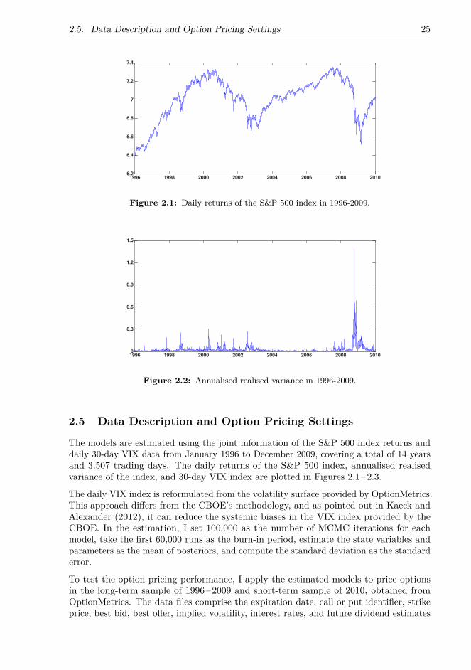
2.5. Data Description and Option Pricing Settings 25
1996 1998 2000 2002 2004 2006 2008 20106.2
6.4
6.6
6.8
7
7.2
7.4
Figure 2.1: Daily returns of the S&P 500 index in 1996-2009.
1996 1998 2000 2002 2004 2006 2008 20100
0.3
0.6
0.9
1.2
1.5
Figure 2.2: Annualised realised variance in 1996-2009.
2.5 Data Description and Option Pricing Settings
The models are estimated using the joint information of the S&P 500 index returns anddaily 30-day VIX data from January 1996 to December 2009, covering a total of 14 yearsand 3,507 trading days. The daily returns of the S&P 500 index, annualised realisedvariance of the index, and 30-day VIX index are plotted in Figures 2.1–2.3.
The daily VIX index is reformulated from the volatility surface provided by OptionMetrics.This approach di�ers from the CBOE’s methodology, and as pointed out in Kaeck andAlexander (2012), it can reduce the systemic biases in the VIX index provided by theCBOE. In the estimation, I set 100,000 as the number of MCMC iterations for eachmodel, take the first 60,000 runs as the burn-in period, estimate the state variables andparameters as the mean of posteriors, and compute the standard deviation as the standarderror.
To test the option pricing performance, I apply the estimated models to price optionsin the long-term sample of 1996–2009 and short-term sample of 2010, obtained fromOptionMetrics. The data files comprise the expiration date, call or put identifier, strikeprice, best bid, best o�er, implied volatility, interest rates, and future dividend estimates

26Chapter 2. Jumps and Volatility Dynamics for the S&P 500 Index:
Conventional MCMC
1996 1998 2000 2002 2004 2006 2008 201010
25
40
55
70
85
100
Figure 2.3: 30-day VIX index in 1996-2009.
based on put-call parity. As in Heston and Nandi (2000), Christo�ersen and Jacobs(2004), and Christo�ersen et al. (2010b), I first use the Wednesday call and put optionsin 1996–2009 (Sample A) to best avoid weekend e�ects and then enhance the sampleby including the option data on Thursday in 1996–2009 (Sample B). To test the optionpricing performance in the short-term sample, I use both the Wednesday and Thursdayoption data (Sample C). Moreover, as suggested by Bakshi et al. (1997), I filter outoptions with prices below 3/8 dollar. Then I remove options with maturities shorter thanone week or longer than one year to reduce the liquidity bias and focus on the short-runoption pricing performance. After filtering, there are 68509, 68322, and 19327 optionsleft in Samples A, B, and C, respectively (details of the option samples are shown inTable 2.2).
When — = 0.5, the models with the SQR variance process are a�ne; consequently, thee�cient FFT can be used to price options. However, since the other models with linearvariance di�usion are non-a�ne, and the FFT is not applicable, for fairness, I use theMonte Carlo method with the technique of antithetic variates to price options. Thenumber of Monte Carlo paths is 50, 000, and the models are discretised at daily frequency.
Another issue to address is how to predict spot variance at each sample date, sincethe spot variance is necessary as the starting value for the variance process in MonteCarlo simulations. Conventionally, the variance is computed from the past return series;however, as pointed out in Kanniainen et al. (2014), this approach reflects only the physicaldynamics, whereas for pricing options, I need information under the risk-neutral measureQ. Furthermore, past return data provide no information about future stock movements,whereas the VIX index is computed from implied volatilities and, thus, naturally indicatesthe investor’s expectation of the future stock market. Kaeck and Alexander (2012) usethe particle filter to generate samples of v
t
at each out-of-sample date from p(vt
|vix
t
, Y
t
)using the fixed parameters estimated from the in-sample data; however, this approachuses the information at time t that, in practice, is not known when option prices arepredicted at time t ≠ 1. In this thesis, I follow the same practice as in Kanniainen et al.(2014): the spot variance at every sample date is extracted from the VIX index value onthe previous date according to Equations 2.26–2.29. Since the squared VIX index can beregarded as a linear function of variance, this approach is extremely fast. According tothe results in Kanniainen et al. (2014), this variance extraction method can improve the
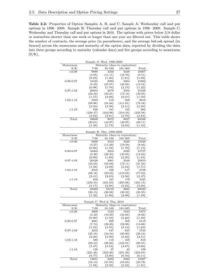
2.5. Data Description and Option Pricing Settings 27
Table 2.2: Properties of Option Samples A, B, and C. Sample A: Wednesday call and putoptions in 1996–2009. Sample B: Thursday call and put options in 1996–2009. Sample C:Wednesday and Thursday call and put options in 2010. The options with prices below 3/8 dollaror maturities shorter than one week or longer than one year are filtered out. This table showsthe number of contracts, the average price (in parentheses), and the average bid-ask spread {inbraces} across the moneyness and maturity of the option data, reported by dividing the datainto three groups according to maturity (calendar days) and five groups according to moneyness(S/K).
Sample A: Wed, 1996-2009
Moneyness Maturity (days to expiration)
S/K 7-90 91-180 181-365 Total
<0.90 9889 3330 3448 16667
(4.05) (11.11) (18.79) (8.51)
{0.83} {1.26} {1.61} {1.08}
0.90-0.97 16425 2993 2384 21802
(8.23) (25.67) (44.02) (14.54)
{0.98} {1.76} {2.15} {1.22}
0.97-1.03 20054 2878 2504 25436
(24.32) (50.21) (73.14) (32.05)
{1.57} {2.08} {2.31} {1.70}
1.03-1.10 2594 510 506 3610
(68.98) (91.84) (111.61) (78.18)
{2.35} {2.38} {2.51} {2.38}
>1.10 638 161 195 994
(236.47) (242.98) (216.34) (233.58)
{2.92} {2.61} {2.76} {2.84}
Total 49600 9872 9037 68509
(20.01) (34.87) (49.97) (26.11)
{1.29} {1.73} {2.03} {1.45}
Sample B: Thu, 1996-2009
Moneyness Maturity (days to expiration)
S/K 7-90 91-180 181-365 Total
<0.90 9299 3310 3320 15929
(4.27) (11.29) (19.59) (8.93)
{0.86} {1.33} {1.70} {1.13}
0.90-0.97 16403 3034 2320 21757
(8.30) (26.43) (43.95) (14.63)
{0.99} {1.80} {2.20} {1.23}
0.97-1.03 20426 3081 2346 25853
(24.03) (50.09) (72.11) (31.50)
{1.58} {2.09} {2.34} {1.71}
1.03-1.10 2705 536 517 3758
(68.16) (93.63) (110.62) (77.63)
{2.41} {2.65} {2.56} {2.47}
>1.10 656 191 178 1025
(222.45) (231.63) (205.08) (221.15)
{3.17} {2.88} {2.94} {3.08}
Total 49489 10152 8681 68322
(20.15) (36.08) (49.52) (26.25)
{1.32} {1.80} {2.08} {1.49}
Sample C: Wed & Thu, 2010
Moneyness Maturity (days to expiration)
S/K 7-90 91-180 181-365 Total
<0.90 4009 1423 1043 6475
(3.42) (10.29) (22.86) (8.06)
{0.90} {1.59} {2.46} {1.30}
0.90-0.97 4681 869 569 6119
(7.74) (28.29) (52.98) (14.86)
{1.24} {2.55} {3.44} {1.63}
0.97-1.03 4252 847 625 5724
(25.16) (54.54) (85.90) (36.14)
{2.20} {3.09} {3.82} {2.51}
1.03-1.10 589 116 105 810
(69.42) (98.82) (122.91) (80.57)
{3.47} {3.53} {4.87} {3.66}
>1.10 120 37 42 199
(221.48) (223.20) (231.20) (223.85)
{6.77} {3.90} {6.16} {6.11}
Total 13651 3292 2384 19327
(16.44) (31.94) (54.65) (23.79)
{1.58} {2.32} {3.22} {1.91}

28Chapter 2. Jumps and Volatility Dynamics for the S&P 500 Index:
Conventional MCMC
option pricing performance of GARCH models beyond that of traditional return-basedvariance updating methods.
As in Christo�ersen et al. (2013), Kaeck and Alexander (2012), and Kanniainen et al.(2014), I compute the root mean square errors (RMSE) from the implied volatility RMSEfrom the sum of the squared di�erence between the theoretical and market option pricesscaled by the inverse Black-Scholes vegas of the options as follows:
VRMSE(�) = 100 ◊ııÙ 1
N
M
ÿ
t,i
3c
i,t
(�, v
t
; T
i
, K
i
) ≠ c
i,t
(Ti
, K
i
)V
t
42
. (2.57)
Here, K
i
is the strike of the ith option at time t, T
i
is the maturity, c
i,t
is the modelprice of the option, and c
t,i
is the market price. Vt,i
is the inverse Black-Scholes vegacomputed on the true market prices of options. Moreover, N
M
=q
M
t=1
N
t
, where N
t
is the number of option prices in the sample at time t, and M is the total number ofdays in the sample. The use of the implied volatility RMSE is motivated by the findingsof Broadie et al. (2007) in that the arithmetic RMSE places more weight on expensivein-the-money and long-maturity options and, conversely, the implied volatility RMSE canadd reasonable weights to options in di�erent moneyness and maturity groups.
2.6 Estimation Results
2.6.1 Parameter EstimatesTables 2.3–2.5 report the parameter estimation results obtained using the joint informationof the S&P 500 index returns and the 30-day VIX from January 1996 to December 2009.
The values of Ÿ
P vary significantly across di�erent models. In the model group SV-P-P-i,the largest Ÿ
P , estimated at 6.1991 (0.5844 as the standard deviation), appears in themodel SV-P-P-1. Compared to the results in previous papers estimating the SV-P-P-0model, my estimation of Ÿ
P is somewhat higher than that in most papers where it rangesfrom 2 to 5. For instance, in Yu et al. (2011), Ÿ
P is 3.3627 (0.6452), estimated withthe MCMC from the S&P 500 index and daily prices of a short-term ATM SPX optionfrom January 1993 to December 1993. In Duan and Yeh (2010), Ÿ
P is 1.9449 (0.6987),estimated with the MLE from the S&P 500 index and the CBOE’s 30-day VIX index fromJanuary 1990 to August 2007. Moreover, in Kaeck and Alexander (2012), Ÿ
P is 3.395(0.328) with the MCMC, estimated from the data of the S&P 500 index and 30-day and360-day VIX indices from January 1990 to December 2004, whereas my sample period isfrom January 1996 to December 2009. One possible explanation relates to the sample dataand estimation method that I use. For instance, Yu et al. (2011) use the index returnsof 1993, when the market was relatively quiet, whereas I adopt longer sample period inwhich there were several big financial crises; this di�erence may lead to the higher Ÿ
P fora more volatile variance path. Another explanation could be the di�erent estimates ofthe jump intensity ⁄ in di�erent papers. In Duan and Yeh (2010), ⁄ is 43.9476 (6.4716),suggesting a quite frequent occurrence of large jumps in a year. Moreover, in Kaeck andAlexander (2012), ⁄ is 5.894 (1.273), almost three times my estimate, and frequent largejumps may obviate a strong mean-reversion to generate large movements.
On the other hand, the inclusion of VG or NIG jumps in returns and variance in thestochastic volatility model can lead to quite di�erent estimates of Ÿ
P . In my estimation,

2.6. Estimation Results 29
Table 2.3: Parameter estimates and DICs of model parameters of the Heston, Bates, andSV-P-P with — = 0.5, 1. The parameters are estimated using the daily spot returns of theS&P 500 index and the reformulated 30-day VIX from January 1996 to December 2009. Theparameter values are the mean of the posteriors as annual decimals. The standard errors are thestandard deviations of the posteriors, reported in parentheses.
Models Heston-0 Heston-1 Bates-0 Bates-1 SV-P-P-0 SV-P-P-1
— 0.5 1 0.5 1 0.5 1
◊
P 0.0403 0.0347 0.0326 0.0212 0.0375 0.0289(0.0057) (0.0048) (0.0029) (0.0023) (0.0054) (0.0064)
Ÿ
P 2.9688 3.4357 4.7392 4.0800 5.8687 6.1991(0.4056) (0.1671) (0.2450) (0.1891) (0.4267) (0.5844)
Ÿ
Q 1.8501 2.0683 4.1184 3.7637 4.9907 5.7795(0.9416) (1.1267) (1.7880) (1.6250) (1.4718) (1.8249)
– 0.3181 1.8546 0.6047 1.8230 0.4152 1.3972(0.0060) (0.0369) (0.0888) (0.1226) (0.7627) (0.7241)
fl -0.7435 -0.7993 -0.8493 -0.8113 -0.8078 -0.8471(0.0056) (0.0103) (0.0702) (0.0097) (0.0603) (0.0133)
÷
s
-2.1615 -2.0133 -1.6083 -0.5095 -1.2440 -1.3763(0.5494) (0.6097) (0.6784) (0.5444) (1.2248) (0.9610)
µ
y
-0.0057 0.0002 -0.0002 -0.0022(0.0018) (0.0003) (0.0005) (0.0010)
µ
Q
y
0.0212 -0.0023 -0.0172 -0.0152(0.0250) (0.0163) (0.0098) (0.0084)
⁄ 31.5728 16.6611 2.0916 2.6678(3.2097) (2.2038) (1.3919) (1.4048)
‡
y
0.0074 0.0213 0.0469 0.0348(0.0009) (0.0012) (0.0084) (0.0052)
fl
J
-0.1975 -0.3185(0.0529) (0.0876)
µ
v
0.0556 0.0609(0.0156) (0.0104)
DIC -39149 -39258 -39383 -43617 -41992 -43874
Ÿ
P in SV-VG-VG-i is the strongest (6.2600 in the SV-VG-VG-0), while in the SV-VG-NIG-i, SV-NIG-VG-i, SV-NIG-i, and SV-NIG-NIG-i, Ÿ
P is much less significant (the lowestŸ
P is 1.0120 in the SV-NIG-0). This is an interesting observation because, intuitively, theinclusion of jumps in variance reduces the need for a strong Ÿ
P to create large changes.This result may suggest that the VG may not be a proper choice for the variance jump,as supported by the insignificant change in the DIC caused by the inclusion of VGvariance jumps, compared to that of the SV-VG-i without variance jumps. Furthermore,the figures of extracted variance jumps in the SV-VG-VG-i confirm that the VG doesnot very actively generate frequent small jumps in variance, and that the magnitudeof large variance jumps generated by the VG is lower than that by the NIG, especiallyduring periods of market turbulence. Moreover, I examine how long-term physical andrisk-neutral variance levels are identified in di�erent model groups. In fact, according tothe VIX index and realised variance in 1996–2009, the long-term physical and risk-neutralannual volatilities are about 16% and 20%, respectively. Overall, the SV-NIG-i, i = 0, 1,and the SV-VG-NIG-i seem more consistent with the data to project realised and expected

30Chapter 2. Jumps and Volatility Dynamics for the S&P 500 Index:
Conventional MCMCTable 2.4: Parameter estimates and DICs of model parameters of the SV-VG, SV-VG-VG, andSV-VG-NIG with — = 0.5, 1. The parameters are estimated using the daily spot returns of theS&P 500 index and the reformulated 30-day VIX from January 1996 to December 2009. Theparameter values are the mean of the posteriors as annual decimals. The standard errors are thestandard deviations of the posteriors, reported in parentheses.
Model SV-VG-0 SV-VG-1 SV-VG-VG-0 SV-VG-VG-1 SV-VG-NIG-0 SV-VG-NIG-1
— 0.5 1 0.5 1 0.5 1
◊
P0.0486 0.0450 0.0175 0.0232 0.0296 0.0301
(0.0014) (0.0008) (0.0025) (0.0052) (0.0037) (0.0022)
Ÿ
P5.3469 2.6819 6.2600 4.9766 2.3209 1.7369
(0.6851) (0.2757) (0.6878) (0.4331) (0.2465) (0.1607)
Ÿ
Q5.3896 1.1632 5.2927 3.6522 1.2462 1.7498
(0.6562) (0.2221) (0.5958) (0.2917) (0.1986) (0.2512)
– 0.6493 2.6504 0.6395 2.7354 0.4489 2.6262
(0.0280) (0.0538) (0.0292) (0.1276) (0.0309) (0.1649)
fl -0.9435 -0.9225 -0.9334 -0.9288 -0.9434 -0.9261
(0.0062) (0.0085) (0.0078) (0.0093) (0.0060) (0.0089)
÷s -2.2801 -1.1632 -2.2931 -2.3841 2.3746 1.2730
(1.3211) (1.1854) (2.1134) (1.0236) (0.6148) (0.6001)
“
Q-0.0182 -0.0003 -0.0900 0.0036 -0.1820 -0.1839
(0.1447) (0.1939) (0.1427) (0.0135) (0.1402) (0.1419)
“ -0.0307 0.0344 0.2264 0.3263 0.1604 0.2248
(0.1394) (0.1863) (0.1303) (0.1458) (0.0548) (0.1260)
‹ < 0.0001 < 0.0001 0.0229 0.0228 0.0229 0.0230
(< 0.0001) (< 0.0001) (0.0004) (0.0004) (0.0005) (0.0005)
‡ 0.0606 0.0566 0.1303 0.1217 0.1043 0.1091
(0.0020) (0.0022) (0.0120) (0.0101) (0.0095) (0.0098)
‡
Q0.1189 0.0910 0.1446 0.1011 0.0755 0.0715
(0.0067) (0.0050) (0.0159) (0.0233) (0.0415) (0.0400)
flv -0.1907 -0.1242 -0.0482 -0.0401
(0.0952) (0.0896) (0.1022) (0.1039)
“
Qv -0.0007 -0.0031 0.0005 -0.0008
(0.0097) (0.0099) (0.0031) (0.0034)
“v 0.0396 0.1000 0.0063 0.0363
(0.0135) (0.0983) (0.0074) (0.0681)
‹
Qv 0.0287 0.0287 0.0939 0.0936
(0.0005) (0.0005) (0.0179) (0.0184)
‡v 0.1953 0.2052 0.0312 0.0680
(0.0057) (0.0227) (0.0163) (0.0025)
DIC -44792 -48144 -43098 -48750 -47202 -53696
variance levels, the SV-P-P-i and the SV-VG-i imply higher variance levels, and theSV-VG-VG-i imply slightly lower levels.
Consistent with the previous literature, the estimates of the physical mean-revertingparameters Ÿ
P and Ÿ
Q imply a negative variance risk premium ÷
v
= Ÿ
Q ≠ Ÿ
P in mostcases. In the SV-P-P-0, the variance risk premium is as large as -0.8780, mainly becauseof the large Ÿ
P . In the Heston-i and SV-VG-VG-i, the variance risk premia are evenmore significant: -1.1187 and -1.3674 for i = 0, 1 in the Heston-i and -0.9673 and -1.3244for i = 0, 1 in the SV-VG-VG-i, respectively. Exceptions of a positive ÷
v
arise in modelsSV-VG-0, SV-VG-NIG-1, SV-NIG-0, and SV-NIG-VG/NIG-i, with 2.9173 being thelargest in the SV-NIG-VG-1 and 0.0129 in the SV-VG-NIG-1. However, most of them,except for those in the SV-NIG-VG-1 and the SV-NIG-0, are insignificant compared to thenegative risk premium values in the other models. A similar result of a small positive ÷
v
also appears in the results of Kaeck and Alexander (2012), who argue that the estimationof the variance process is plausible because the VIX-implied long-term variance level intheir sample period is successfully estimated, which is also done in my estimation. They

2.6. Estimation Results 31
Table 2.5: Parameter estimates and DICs of model parameters of the SV-NIG, SV-NIG-VG,and SV-NIG-NIG with — = 0.5, 1. The parameters are estimated using the daily spot returns ofthe S&P 500 index and the reformulated 30-day VIX from January 1996 to December 2009. Theparameter values are the mean of the posteriors as annual decimals. The standard errors are thestandard deviations of the posteriors, reported in parentheses.
Model SV-NIG-0 SV-NIG-1 SV-NIG-VG-0 SV-NIG-VG-1 SV-NIG-NIG-0 SV-NIG-NIG-1
— 0.5 1 0.5 1 0.5 1
◊
P0.0115 0.0266 0.0167 0.0451 0.0128 0.0452
(0.0059) (0.0041) (0.0011) (0.0048) (0.0027) (0.0100)
Ÿ
P1.0120 2.3512 3.0015 2.2694 1.1531 1.3045
(0.4810) (0.4118) (1.0950) (0.2257) (0.1570) (0.3451)
Ÿ
Q2.6163 0.9687 3.7093 5.1867 1.6379 1.7273
(1.5738) (0.6880) (1.7368) (1.8835) (1.6176) (1.3073)
– 0.3376 2.5347 0.4891 2.5039 0.3154 2.2123
(0.0101) (0.0649) (0.0122) (0.1305) (0.0224) (0.1127)
fl -0.9495 -0.9326 -0.9479 -0.9313 -0.9489 -0.9367
(0.0011) (0.0088) (0.0026) (0.0087) (0.0018) (0.0078)
÷s 0.1511 -0.0699 -1.3819 -0.5883 -1.2290 -1.3166
(1.0707) (1.0341) (0.6887) (0.6835) (0.7557) (0.6827)
“
Q-0.2031 -0.1947 -0.1854 -0.1768 -0.3740 -0.1762
(0.1425) (0.1412) (0.1373) (0.1416) (0.2299) (0.1361)
“ 0.1954 0.0722 0.6571 0.5233 0.4280 0.2207
(0.5910) (0.1293) (0.9566) (0.9952) (1.0015) (0.9343)
‹
Q6.7768 3.3669 11.5623 12.3703 46.4268 12.7099
(0.7422) (0.5523) (0.9656) (1.1066) (2.5926) (1.2125)
‡ 0.2154 0.1506 0.4582 0.3091 0.2584 0.1944
(0.0151) (0.0245) (0.0326) (0.0645) (0.1546) (0.0847)
flv -0.0327 -0.1554 -0.1352 -0.1110
(0.0352) (0.1186) (0.0683) (0.1353)
“
Qv -0.0027 -0.0008 0.0427 -0.0029
(0.0976) (0.0958) (0.2941) (0.0922)
“v 0.3753 0.0559 0.0380 0.0619
(0.0521) (0.0973) (0.0432) (0.0903)
‹
Qv 0.0287 0.0287 0.2250 0.2196
(0.0005) (0.0005) (0.1221) (0.0997)
‡v 0.0300 0.1002 0.0566 0.1223
(0.0009) (0.0200) (0.0036) (0.0129)
DIC -50861 -51700 -49835 -50314 -45757 -49526
also postulate that the insignificant ÷
v
may result from a relatively flat variance termstructure, which increases the di�culty of correctly estimating the variance risk premium÷
v
, as pointed out in Broadie et al. (2007). The estimation of the variance risk premiumin returns, that is, ÷
s
, in all models except for the SV-VG-NIG-i and the SV-NIG-0,supports the economic interpretation of a negative ÷
s
. However, in most models, thestandard errors of ÷
s
are large, suggesting that ÷
s
is quite di�cult to estimate.
The leverage e�ect is captured by all the models, because the correlation factor fl isestimated to be negative. However, compared to fl in the Bates-i and SV-P-P-i, in othermodels with VG or NIG return jumps, fl is much closer to -1, ranging from ≠0.9225 inthe SV-VG-1 to ≠0.9495 in the SV-NIG-0 and suggesting a stronger negative interactionbetween changes in spot returns and variance. This can be explained by the di�erentjump structures: in models without jumps in variance, the correlation between changesin spot variance and returns can only be captured by the correlation between di�usionterms; in models with VG/NIG jumps in variance, the correlation between J
y
and J
v
isrelatively weak, whereas in the SV-P-P-i, i = 0, 1, the variance jumps directly a�ect thejump in returns by J
Y
≥ N(µy
+ fl
J
J
v
, ‡
2
y
).

32Chapter 2. Jumps and Volatility Dynamics for the S&P 500 Index:
Conventional MCMC
In models with VG/NIG variance jumps, fl
v
remains negative, from -0.2 to -0.03, suggestinga negative correlation of jumps in returns and variance, but the correlation between thejumps is not as strong as that between di�usions. In models with di�erent jump types inreturns and variance, fl
v
is negligible, which is plausible because di�erent types of Lévyjumps with distinctive features and behaviour are used in returns and variance.Let us discuss now how these models seek to account for the long-memory e�ect. Here,two quantities specific to the models are considered, namely, conditional variance E
P
t
[vt+d
]and conditional variance of variance var
P
t
[vt+d
], to illustrate how under the physicalmeasure P , the current variance a�ects the future variance after d years in di�erentmodels. E
t
[vt+d
] and var
t
[vt+d
] are calculated as follows:
E
P
t
[vt+d
] = e
≠Ÿ
Pd
v
t
+ Ÿ
P
◊
P + M
v
Ÿ
P
11 ≠ e
≠Ÿ
Pd
2, (2.58)
var
P
t
[vt+d
] = –
2
Ÿ
P
1e
≠Ÿ
Pd ≠ e
≠2Ÿ
Pd
2v
t
+ var
P (Jv,t
)Ÿ
P
11 ≠ e
≠2Ÿ
Pd
2(2.59)
+–
2(ŸP
◊
P + M
v
)2(ŸP )2
(1 ≠ e
≠Ÿ
Pd)2
, (2.60)
where var
P (Jv,t
) is the variance of the variance jumps. The above equations show thatthe conditional expectation of future variance is a�ected by the current level with thecoe�cient e
≠Ÿ
Pd; thus, a higher Ÿ
P leads to a smaller correlation between v
t
and v
t+d
.Furthermore, with other conditions being the same, a low Ÿ
P increases the conditionalvariance of variance var
t
[vt+d
].Although the choice of J
v
and — does not directly a�ect the long-memory e�ect, I noticethat Ÿ
P is quite sensitive to J
v
and – varies with —. Generally, in the SV-VG-VG-i andthe SV-P-P-i, Ÿ
P is the highest, followed by that in the Bates-i, SV-VG-i, and Heston-i,and the lowest in the SV-VG-NIG-i, SV-NIG-i, and SV-NIG-VG/NIG-i, suggesting thatwith the same —, models with an NIG jump in returns or variance show the strongest long-memory e�ect, and the SV-VG-VG-i and the SV-P-P-i show the weakest. To illustrate,the coe�cient e
≠Ÿ
Pd when d = 1/12 is 0.5935 in the SV-VG-VG-0, and after one year, it
drops to 0.0019; in the SV-NIG-0, the one-month e
≠Ÿ
Pd is 0.9191, and the one-year e
≠Ÿ
Pd
is still high, reaching 0.3635. Furthermore, across di�erent model groups, a higher — leadsto a significantly higher –, and although the value of – does not a�ect the conditionalvariance, it raises the conditional variance of variance as it increases.Next, I move to the behaviour of jumps in returns and variance. Extracted jumps inreturns and variance for each model are plotted in Figures 2.4–2.15. Since there areapparent di�erences between di�erent model groups and almost the same patterns withinthe same model group, I include only the figures of jumps in models with — = 1 in eachmodel group. The figures of extracted jumps in returns and variance show clear di�erencesin jump behaviour between finite-activity and infinite-activity jumps. The SV-P-P-1has 26 jumps with an absolute size of over 0.005; in fact, they are almost all downsidejumps, which is consistent with the observations. More interestingly, when jumps withabsolute size larger than 0.01 are extracted, 17 jumps are left with several waves of largejumps occurring in 1998, 2000, 2007, and 2008, covering the several financial crises in thesample period of 1996–2009. Furthermore, there is a clear negative correlation betweenthe jumps in returns and in variance.Notably, in the SV-P-P-i, both µ
y
and µ
Q
y
are estimated with large standard errors. Aspointed out in Eraker (2004), the di�culty of estimating µ
y
lies in that this parameter

2.6. Estimation Results 33
can be identified only from the index return; however, if only a few return jumps areobserved, it may be hard to estimate µ
y
as the expected mean of the jumps. Moreover,as shown in Kaeck and Alexander (2012), since only the squared value (µQ
y
)2 enters theformula of the model-implied VIX, µ
Q
y
is bi-modal, and the algorithm cannot determineits sign.To deal with the di�culty of estimating jump-related parameters, Kaeck and Alexan-der (2012) assume a zero jump risk premium by setting the risk-neutral jump-relatedparameters identical to the physical ones, because they notice that the jump premium„
Q
J
(≠i) ≠ „
P
J
(≠i) is very insignificant. In the estimation, I first use di�erent jump-relatedparameters under P and Q, and my estimation results of µ
y
are similar to those in Kaeckand Alexander (2012). However, the absolute sizes of the risk-neutral parameters µ
Q
y
inthe SV-P-P-i are much larger than the physical µ
y
. The di�erence is also found in, forexample, Eraker (2004) and Yu et al. (2011), implying from the investors’ point of view astrong uncertainty about future jump size.To further probe into the problem of estimating µ
y
and µ
Q
y
, I follow the practice of Kaeckand Alexander (2012) by setting µ
Q
y
= µ
y
and updating other jump-related parameters,including ⁄, ‡
y
, fl
J
, and µ
v
, only according to the information about index returns. Theresults reveal that for the SV-P-P-i, when µ
v
is close to its previous estimates, µ
y
is moresignificant and ‡
y
is more than 10 times its previous estimate. The larger expected meanand variance of return jumps can be explained by a smaller ⁄: about 0.25 jumps peryear, estimated under the uniform prior, daily ⁄ ≥ U(0, 1). When this new estimationresult is used, both the DICs and option pricing performance deteriorate. Therefore, inthis chapter, I only report the estimates obtained on the basis of the joint information ofindex returns and VIX.3
The behaviour of return jumps in the models SV-NIG-i resembles closely that of modelsSV-VG-i, except that there are many more small jumps, which is expected because theNIG is of infinite variation. For models with VG return jumps, the expected jump size“
Q is bi-modal, because only (“Q)2 enters the formula of the VIX index. Thus, to obtainmore plausible results in the estimation, I choose priors for “
Q by restricting its value toeither positive or negative. However, “ and “
Q are still estimated with relatively largestandard errors. One could argue that the VIX does not contain useful information inthis regard, and that option data should be used instead of the VIX. However, in Yu et al.(2011), where the model SV-VG-0 is estimated from the index and option data, theseparameters continue to be estimated with quite large standard errors: 0.0256(0.0315) for“ and 0.0030(0.0056) for “
Q in the SV-VG-0. When the other jump-related parametersare estimated with reasonable standard errors, the standard errors of parameters µ
y
,µ
Q
y
, “, and “
Q are relatively large, and this suggests that the parameters measuring theexpected mean of jumps are di�cult to identify. One possible solution could be to makethese parameters time varying, and they may depend on the level of variance, as assumedin Bates (2012) and Eraker (2004).
3The estimates of ⁄, ‡y , flJ , and µv reported in Table 2.3 are computed as the mean of the posteriors,estimated from the joint information of the VIX and index returns, and when they are estimated onlyfrom index data, as in Kaeck and Alexander (2012), their estimates are quite di�erent. The di�erence inthe estimates of jump-related parameters may suggest that the models are not consistent with the marketdata: the SV-P-P-i fail to jointly capture the physical dynamics implied by the index and the risk-neutraldynamics implied by the VIX. Then I conduct a simple simulation study to verify this, simulating five-yeardata of the index and VIX under the Bates-1 and SV-P-P-1 models and first estimating the models withsimulated index data and then with the simulated index and VIX data. I notice that in both estimationexperiments, the extracted jumps in returns and variance almost coincide with the simulated jumps, andthe estimation results of ⁄, ‡y , flJ , and µv are very close to the corresponding true values.
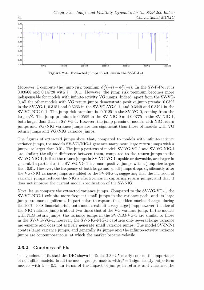
34Chapter 2. Jumps and Volatility Dynamics for the S&P 500 Index:
Conventional MCMC
1997/12 1999/12 2001/12 2003/12 2005/12 2007/12 2009/12−0.07
−0.06
−0.05
−0.04
−0.03
−0.02
−0.01
0
0.01
0.02
Figure 2.4: Extracted jumps in returns in the SV-P-P-1
Moreover, I compute the jump risk premium „
Q
J
(≠i) ≠ „
P
J
(≠i). In the SV-P-P-i, it is0.03568 and 0.14728 with i = 0, 1. However, the jump risk premium becomes moreindispensable for models with infinite-activity VG jumps. Indeed, apart from the SV-VG-0, all the other models with VG return jumps demonstrate positive jump premia: 0.0322in the SV-VG-1, 0.3151 and 0.3263 in the SV-VG-VG-0, 1, and 0.3449 and 0.3794 in theSV-VG-NIG-0, 1. The jump risk premium is -0.0125 in the SV-VG-0, coming from thelarge “
Q. The jump premium is 0.0588 in the SV-NIG-0 and 0.0775 in the SV-NIG-1,both larger than that in SV-VG-1. However, the jump premia of models with NIG returnjumps and VG/NIG variance jumps are less significant than those of models with VGreturn jumps and VG/NIG variance jumps.
The figures of extracted jumps show that, compared to models with infinite-activityvariance jumps, the models SV-VG/NIG-1 generate many more large return jumps with ajump size larger than 0.01. The jump patterns of models SV-VG-VG-1 and SV-VG-NIG-1are similar; the slight di�erence between them, compared to the return jumps in theSV-VG-NIG-1, is that the return jumps in SV-VG-VG-1, upside or downside, are larger ingeneral. In particular, the SV-VG-VG-1 has more positive jumps with a jump size largerthan 0.01. However, the frequency of both large and small jumps drops significantly afterthe VG/NIG variance jumps are added to the SV-NIG-1, suggesting that the inclusion ofvariance jumps reduces the NIG’s e�ectiveness in capturing return jumps, and that itdoes not improve the current model specification of the SV-NIG.
Next, let us compare the extracted variance jumps. Compared to the SV-VG-VG-1, theSV-VG-NIG-1 exhibits more frequent small jumps in the variance path, and its largejumps are more significant. In particular, to capture the sudden market changes duringthe 2007–2008 financial crisis, both models exhibit a very large jump; however, the size ofthe NIG variance jump is about two times that of the VG variance jump. In the modelswith NIG return jumps, the variance jumps in the SV-NIG-VG-1 are similar to thosein the SV-VG-VG-1; however, the SV-NIG-NIG-1 captures only several large variancemovements and does not actively generate small variance jumps. The model SV-P-P-1creates large variance jumps, and generally its jumps and the infinite-activity variancejumps are contemporaneous, at which the market became volatile.
2.6.2 Goodness of Fit
The goodness-of-fit statistics DIC shown in Tables 2.3–2.5 clearly confirm the importanceof non-a�ne models. In all the model groups, models with — = 1 significantly outperformmodels with — = 0.5. In terms of the impact of jumps in returns and variance, the
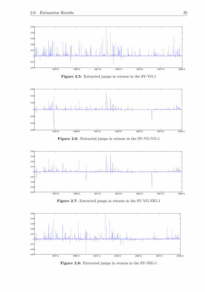
2.6. Estimation Results 35
1997/12 1999/12 2001/12 2003/12 2005/12 2007/12 2009/12−0.02
−0.01
0
0.01
0.02
0.03
0.04
0.05
Figure 2.5: Extracted jumps in returns in the SV-VG-1
1997/12 1999/12 2001/12 2003/12 2005/12 2007/12 2009/12−0.06
−0.04
−0.02
0
0.02
0.04
0.06
Figure 2.6: Extracted jumps in returns in the SV-VG-VG-1
1997/12 1999/12 2001/12 2003/12 2005/12 2007/12 2009/12−0.04
−0.03
−0.02
−0.01
0
0.01
0.02
0.03
0.04
Figure 2.7: Extracted jumps in returns in the SV-VG-NIG-1
1997/12 1999/12 2001/12 2003/12 2005/12 2007/12 2009/12−0.03
−0.02
−0.01
0
0.01
0.02
0.03
0.04
0.05
Figure 2.8: Extracted jumps in returns in the SV-NIG-1

36Chapter 2. Jumps and Volatility Dynamics for the S&P 500 Index:
Conventional MCMC
1997/12 1999/12 2001/12 2003/12 2005/12 2007/12 2009/12−0.04
−0.03
−0.02
−0.01
0
0.01
0.02
0.03
0.04
Figure 2.9: Extracted jumps in returns in the SV-NIG-VG-1
1997/12 1999/12 2001/12 2003/12 2005/12 2007/12 2009/12−0.04
−0.03
−0.02
−0.01
0
0.01
0.02
0.03
Figure 2.10: Extracted jumps in returns in the SV-NIG-NIG-1
1997/12 1999/12 2001/12 2003/12 2005/12 2007/12 2009/120
0.05
0.1
0.15
0.2
0.25
0.3
0.35
Figure 2.11: Extracted jumps in variance in the SV-P-P-1
1997/12 1999/12 2001/12 2003/12 2005/12 2007/12 2009/12−0.04
−0.02
0
0.02
0.04
0.06
0.08
0.1
Figure 2.12: Extracted jumps in variance in the SV-VG-VG-1

2.6. Estimation Results 37
1997/12 1999/12 2001/12 2003/12 2005/12 2007/12 2009/12−0.1
−0.05
0
0.05
0.1
0.15
0.2
0.25
Figure 2.13: Extracted jumps in variance in the SV-VG-NIG-1
1997/12 1999/12 2001/12 2003/12 2005/12 2007/12 2009/12−0.06
−0.04
−0.02
0
0.02
0.04
0.06
0.08
Figure 2.14: Extracted jumps in variance in the SV-NIG-VG-1
1997/12 1999/12 2001/12 2003/12 2005/12 2007/12 2009/12−0.02
−0.01
0
0.01
0.02
0.03
0.04
0.05
Figure 2.15: Extracted jumps in variance in the SV-NIG-NIG-1
Heston-i, Bates-i, and SV-P-P-i perform the worst, with the best model class being theSV-VG-NIG-i, followed by model classes SV-NIG-i, SV-NIG-VG/NIG-i, SV-VG-i, andSV-VG-VG-i. The large di�erence in the DIC between the benchmark models (Heston-i,Bates-i, and SV-P-P-i) and the other models provides strong evidence of the inclusionof VG/NIG jumps in the return process, which produces a better fit than not onlythe di�usion model but also models with compound Poisson jumps. In particular, theinclusion of NIG variance jumps in the SV-VG can further improve its goodness of fit. Asurprising observation is that the inclusion of VG variance jumps (SV-VG-VG-i) does notresult in an obviously lower DIC than the SV-VG-i. This implies that the VG-type jumpmay not be an appropriate choice for the variance process, at least compared to the NIGjump. In the models with NIG return jumps, the inclusion of variance jumps, in contrast,worsens the goodness of fit due to over-fitting, suggesting that no extra infinite-activityjumps are necessary in variance for the SV-NIG models.
38Chapter 2. Jumps and Volatility Dynamics for the S&P 500 Index:
Conventional MCMC
However, if we take a closer look at the di�erence in DICs caused by the linear varianceprocess and inclusion of jumps, there is mixed evidence about the relative importanceof these two specifications. The goodness-of-fit performance becomes much better afterthe compound Poisson jumps in returns are replaced with VG/NIG jumps, even if acomparison is made between the Bates-1/SV-P-P-1 and the SV-VG-0/SV-NIG-0. Theinclusion of proper NIG-type variance jumps can further improve the fit, but this can beachieved only after changing the variance process from SQR to the linear type. In terms ofmodelling variance dynamics, the VG jump has proved not to be the best choice, as it failsto markedly improve the SV-VG models. In general terms, linear variance specificationcan improve the fit within the same magnitude, but the inclusion of appropriate jumpsin returns and variance can significantly lower the DICs. In other words, the inclusionof VG/NIG return jumps is the first priority, followed by the specification of the linearvariance process, and then the inclusion of the “right” jump in variance.
I have one comment about the di�erence in DICs. The di�erence between the highest andlowest DICs across all models is 14,547. Within the same model group, the di�erences inDICs caused by the di�erent — range from 109 in the Heston-i to 7,354 in the SV-VG-NIG-i, and the di�erences caused by the use of infinite-activity jumps in returns or varianceare about 3,000-5,000. However, as pointed out in Spiegelhalter et al. (2002), a smalldi�erence in the DICs can be significant and, by contrast, my result is surprisingly strong.I also compare the DICs with Kaeck and Alexander (2012), because we discuss somecommon models, and because our sample data sets are quite similar. In their paper, theycompare one-factor and two-factor models with — = 0.5 or 1 or flexible —, and the largestDIC di�erence is 44,511, caused by the use of a second factor. However, the di�erencecaused by — in one-factor models, which is about 600, is quite small compared to mine,whereas in two-factor models, the di�erence caused by a di�erent — is an average of 3,000.In one-factor models, the di�erence in DICs caused by the use of compound Poissonjumps in returns and variance is about 900, and in two-factor models it is about 3,000,on average, derived from the penalty of overfitting with jump components. Consideringthat Kaeck and Alexander (2012) use the VIX term structure of 30 and 360 days, thesecond factor plays an important role in capturing the long-term behaviour of variance,whereas in the short term, jumps can help create frequent fluctuations in returns andvariance, which may explain the relatively large di�erence in DICs caused by jumps inmy estimation. Another possible reason is errors in the Monte Carlo sampling. To studythis, I re-estimate the SV-P-P-0, 1 and notice that the Monte Carlo sampling seems tocause small di�erences in the DIC, but they are insignificant compared to those betweendi�erent models.
2.6.3 Fit to the VIX
Table 2.6 reports the estimates of the correlation factor fl
Á
and the scaled factor ‡
Á
.Among all models, the di�erence in fl
Á
and ‡
Á
is negligible; therefore, no inference canbe drawn regarding the performance of fit to the VIX. Across all the models, fl
Á
is closeto 1, suggesting a significant positive autocorrelation between the VIX pricing errors onneighbouring days. A similar observation is made in Kanniainen et al. (2014), where anadditive error model with auto-regressive disturbances is used for VIX pricing errors,and also in Yu et al. (2011), which, like me, use the multiplicative error model withauto-regressive disturbances to model the errors between the market prices and thetheoretical values of options on neighbouring days. The autocorrelation factor in bothpapers is close to 1. With the same error model, but for variance swap rates, the result

2.6. Estimation Results 39
Table 2.6: Estimates of flÁ and ‡Á in the Heston, Bates, SV-P-P, SV-VG, SV-VG-VG, SV-VG-NIG, SV-NIG, SV-NIG-VG, and SV-NIG-NIG with di�erent choices of —. The parametersare estimated using daily spot returns of the S&P 500 index and the reformulated 30-day VIXfrom January 1996 to December 2009. The parameter values are the mean of the posteriors asannual decimals. The standard errors are the standard deviations of the posteriors, reported inparentheses.
Models Heston-0 Heston-1 Bates-0 Bates-1 SV-P-P-0 SV-P-P-1
fl
Á
0.9870 0.9919 0.9800 0.9832 0.9988 0.9968(0.0032) (0.0025) (0.0034) (0.0040) (0.0020) (0.0015)
‡
Á
0.0371 0.0344 0.0514 0.0339 0.0273 0.0305(0.0008) (0.0010) (0.0017) (0.0009) (0.0012) (0.0031)
Models SV-VG-0 SV-VG-1 SV-VG-VG-0 SV-VG-VG-1 SV-VG-NIG-0 SV-VG-NIG-1
fl
Á
0.9861 0.9816 0.9898 0.9835 0.9840 0.9828(0.0033) (0.0041) (0.0043) (0.0045) (0.0221) (0.0085)
‡
Á
0.0347 0.0333 0.0352 0.0343 0.1636 0.0377(0.0008) (0.0009) (0.0009) (0.0011) (0.2039) (0.0039)
Model SV-NIG-0 SV-NIG-1 SV-NIG-VG-0 SV-NIG-VG-1 SV-NIG-NIG-0 SV-NIG-NIG-1
fl
Á
0.9955 0.9780 0.9789 0.9789 0.9923 0.9786(0.0020) (0.0034) (0.0052) (0.0050) (0.0055) (0.0086)
‡
Á
0.0410 0.0342 0.0428 0.0350 0.0435 0.0387(0.0008) (0.0011) (0.0007) (0.0016) (0.0068) (0.0023)
obtained in Amengual (2009) di�ers slightly from mine. In their paper, the values offl
Á
, regardless of the choice of models, are U-shaped: close to zero in three months andmuch higher in one month or two years. In particular, their one-month fl
Á
ranges from0.437 to 0.684. However, using the same error model, Kaeck and Alexander (2012) obtainquite di�erent results: fl
Á
is almost zero for the 30-day VIX index, and for the 360-dayVIX index, it shows large positive values for one-factor models and again nearly zerovalues for two-factor models, suggesting weak autocorrelation in the error terms. Thismixed di�erence between some papers and mine may result from our di�erent sources ofinformation or di�erent choices of models. In particular, I compare the model-implied VIXand the market VIX and notice that there tends to be strong, positive autocorrelationbetween daily VIX pricing errors when there are significant jumps in the path of themarket VIX, that is, when the stock market became volatile. This positive autocorrelationmay come from a variance path di�erent from the pattern of the VIX index,4 and suggeststhat if the data sample for estimation covers periods when the market was turbulent,the autocorrelation parameter fl
Á
could be more significant than that estimated fromthe data sample that comes from a period during which the market was relatively quiet.Moreover, the large positive autocorrelation between daily errors may also suggest thatmodels do not perform well in fitting the VIX and the index at the same time. Therefore,a near random-walk error process with a large positive autocorrelation factor could help
4It may be because I extract the variance using the joint information of the index return and VIXindex.

40Chapter 2. Jumps and Volatility Dynamics for the S&P 500 Index:
Conventional MCMC
to capture the deviation between the market VIX and model-implied VIX.5 Furthermore,the choice of estimation method counts. In my research, the variance path is extractedwith the random-walk MH algorithm and in Kaeck and Alexander (2012) with the ARMSalgorithm to estimate the variance. In my other research with the MCMC, I observe thatmethods of extracting the variance dynamics might a�ect the model-implied VIX. If amethod tends to extract a more volatile volatility curve, the model-implied VIX is morevolatile; consequently, daily errors between the model-implied and market VIX mightvary widely from day to day, implying a lower autocorrelation coe�cient.
2.6.4 Option Pricing PerformanceIn this section, I address the question of whether infinite-activity Lévy jumps can improvethe option pricing performance. I answer this question under both a�ne (SQR) andnon-a�ne (linear) volatility di�usions. Table 2.7 reports the option RMSEs of all themodels for three samples: Sample A comprising the Wednesday options from January1996 to December 2009, Sample B comprising the Thursday options from January 1996to December 2009,6 and Sample C comprising the Wednesday and Thursday options fromJanuary 2010 to December 2010. The test7 allows me to analyse the role of di�erentmodel specifications in option pricing, and it further verifies the e�ectiveness of the useof the VIX index in estimating the models’ risk-neutral dynamics.
As for the role of jumps, I first examine option performance with a�ne models and thennon-a�ne models.
Importance of Infinite-Activity Jumps under A�ne (SQR) Volatility Di�usion
In pricing options from the long-term Samples A and B, the SV-NIG-0 achieves thebest result with Sample A, and its result with Sample B is very close to the best oneobtained by the SV-NIG-VG-0. The superior performance of the a�ne model with NIGreturn jumps over the Heston-0, Bates-0, and SV-P-P-0 suggests that the inclusion ofNIG return jumps can significantly improve the performance of the di�usion model inpricing options in the long-term sample period, and that it is more appropriate than theinclusion of compound Poisson jumps. However, there is mixed evidence about the roleof variance jumps. On the one hand, the inclusion of VG variance jumps improves thepricing performance of the SV-NIG-0 with Sample B, and the SV-VG-NIG-0 achieves thethird best performance with Samples A and B, better than the SV-VG-0; on the otherhand, the model specifications of the SV-VG-VG-0 and SV-NIG-NIG-0 make the resultsdeteriorate, and this suggests that more complex models do not necessarily lead to betterresults. The SV-VG-0 achieves a result comparable to that of the Heston-0 and Bates-0with Samples A and B, but it achieves the best option pricing performance with theshort-term Sample C. Surprisingly, the SV-NIG-0, which is among the two best modelswith Samples A and B, produces the worst result with Sample C, while the SV-VG-NIG-0and SV-NIG-VG-0 maintain their performance. Another interesting observation is that
5In future research, it would be interesting to preset the autocorrelation factor flÁ to a lower value,which may lead to the model-implied VIX further coinciding with the market VIX.
6The use of Thursday option data is aimed at enhancing the evidence of model performance, motivatedby Christo�ersen et al. (2010a), where the Wednesday options are used for estimation and the Thursdayoptions for out-of-sample analysis.
7As argued in Christo�ersen et al. (2010b), the option pricing test is out-of-sample even if thedata sample used for estimation is from the same period as the option sample. Therefore, by followingChristo�ersen et al. (2010b), all option Samples A, B, and C can be considered out-of-sample because nooption data are directly used for the estimation.

2.6. Estimation Results 41
Table 2.7: Option VRMSEs for a�ne (i = 0) and non-a�ne (i = 1) models. Sample A: Optionson Wednesdays from January 1996 to December 2009. Sample B: Options on Thursdays fromJanuary 1996 to December 2009. Sample C: Options on Wednesdays and Thursdays from January2010 to December 2010. Options with prices below 3/8 dollar or maturities shorter than oneweek or longer than one year are filtered out. I compute the option prices using the Monte Carlomethod with the technique of antithetic variates. The number of Monte Carlo paths is 50, 000,and the models are discretised at daily frequency. In each sample, the bolded and italic numbersare the lowest and highest VRMSEs, respectively, and the models are ranked according to theirperformance in Sample A.
model i A B CSV-NIG 0 4.4506 5.0538 5.3543SV-NIG-VG 0 4.5488 5.0458 4.8854SV-VG-NIG 0 4.8204 5.1926 4.7558Heston 0 4.8397 5.4596 5.5918Bates 0 4.8491 5.3973 5.0740SV-VG 0 4.8855 5.3167 4.5432SV-NIG-NIG 0 5.1724 5.6865 5.4251SV-P-P 0 5.1917 5.6332 5.0015SV-VG-VG 0 6.4875 6.6092 5.3300
model i A B CSV-NIG 1 3.2988 3.8806 3.4939SV-VG-NIG 1 3.6579 4.1553 3.7446SV-VG 1 3.7863 4.2534 3.7698Heston 1 3.8896 4.4093 4.5014Bates 1 3.9211 4.4643 4.7496SV-NIG-NIG 1 4.0437 4.4377 4.0404SV-VG-VG 1 4.1851 4.6071 4.0656SV-NIG-VG 1 4.3431 4.4265 4.1746SV-P-P 1 4.6311 4.9499 4.4725
the SV-P-P-0 outperforms the Heston-0 and Bates-0, and ranks fourth best with SampleC. This observation shows that with the a�ne variance dynamics, the performance ofdi�erent return jump specifications is not stable with di�erent samples. Overall, theperformance of infinite-activity jump models is mixed between the di�erent option pricedata samples. The models’ mixed, inconsistent performance in pricing options in thelong-term and short-term samples suggests that the use of (unrealistic) a�ne variancedynamics may negatively a�ect the identification of the other model components andlead to an unstable pricing performance between di�erent samples.
Importance of Infinite-Activity Jumps under Non-A�ne (linear) Volatility Di�usion
In contrast to the mixed performance of the a�ne models with di�erent samples, with thenon-a�ne variance dynamics, the SV-NIG-1, SV-VG-NIG-1, and SV-VG-1 with infinite-activity jumps are always the best three models for all the samples, and their optionpricing performance is much better than the best results obtained by the a�ne models.This observation shows that infinite-activity jumps, especially NIG return jumps, shouldbe used with non-a�ne variance dynamics, instead of finite-activity compound Poissonjumps. Similar to those with a�ne models, the results with non-a�ne models imply that

42Chapter 2. Jumps and Volatility Dynamics for the S&P 500 Index:
Conventional MCMCTable 2.8: Option VRMSEs for models in di�erent maturity groups. Sample: Options onWednesdays from January 2010 to December 2010. Options with prices below 3/8 dollar ormaturities shorter than one week or longer than one year are filtered out. The option prices arecomputed using the Monte Carlo method with the technique of antithetic variates. The numberof Monte Carlo paths is 50, 000, and the models are discretised at daily frequency.
Maturity # Options Heston-0 Heston-1 Bates-0 Bates-1 SV-P-P-0 SV-P-P-1
7 - 90 6926 6.1884 5.0640 5.7554 4.8434 5.4191 4.753091 - 180 1663 4.9269 3.2591 4.2301 3.7321 4.6767 3.9233181 - 365 1187 3.6833 2.5166 3.2569 4.9606 4.1484 3.6546
Maturity # Options SV-VG-0 SV-VG-1 SV-VG-VG-0 SV-VG-VG-1 SV-VG-NIG-0 SV-VG-NIG-1
7 - 90 6926 5.0464 4.1744 5.6661 4.3562 5.3376 4.089491 - 180 1663 3.5736 2.3744 4.4217 2.7691 4.1223 2.1997181 - 365 1187 3.0746 2.6338 4.2983 2.8392 3.4604 2.8178
Maturity # Options SV-NIG-0 SV-NIG-1 SV-NIG-VG-0 SV-NIG-VG-1 SV-NIG-NIG-0 SV-NIG-NIG-1
7 - 90 6926 5.7412 3.9579 5.5780 4.4826 5.7293 4.539291 - 180 1663 4.3054 2.4266 3.9773 3.4209 5.1226 2.6424181 - 365 1187 5.7584 2.9047 4.0908 4.0810 5.8349 2.4138
the inclusion of jumps in variance does not necessarily lead to an improved option pricingperformance. The choice of jump type matters, and the impact of the variance jumps isnot as significant as that of the return jumps. Indeed, the parsimonious SV-NIG-1 clearlyoutperforms all the other models, including the more complex models with variancejumps, and the inclusion of either VG or NIG variance jumps in the SV-NIG-1 distortsthe pricing results. This implies that the NIG return jump is su�cient for capturing thejump risks under the risk-neutral measure without variance jumps, and that extra modelspecifications seem to destabilise the model estimation.
Overall, complicated models with extra parameters do not necessarily yield a betteroption pricing performance. For example, in Eraker (2004), with the parameters directlyestimated from returns and option data, the in-sample option pricing performance of theBates-0 model is comparable to that of the augmented SV-P-P-0, and even better thanSV-P-P-0 in terms of out-of-sample performance. Importantly, I do not directly calibratethe models to the option data, which makes it possible for the SV-NIG-1 to have betterresults with Samples A and B than the SV-NIG-NIG/VG-1. However, if one prefers toinclude jumps in variance, the specification of the SV-VG-NIG is best for both a�ne andnon-a�ne variance dynamics.
In all samples, the specification of the non-a�ne linear variance process can significantlyreduce the option VRMSE across di�erent model groups, up to 35% in the SV-VG-VG-i inSample A, and 23% and 36% in the SV-NIG-i in Samples B and C, respectively. In general,the superior performance of the linear variance process across di�erent model groupsstrongly suggests that to capture the risk-neutral dynamics, the variance process with— = 1 is preferable to the SQR variance process. More importantly, as highlighted above,with the non-a�ne variance dynamics, the performance of return jumps is consistentwith di�erent option samples, whereas with the a�ne dynamics, the results are mixed.This suggests that the use of non-a�ne dynamics both improves model performance andstabilises it.
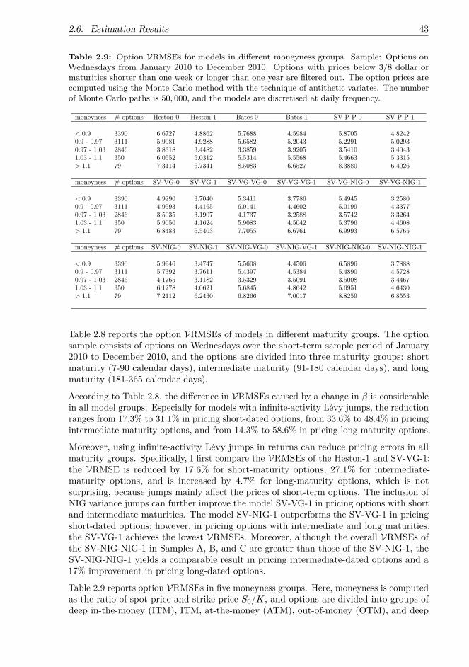
2.6. Estimation Results 43
Table 2.9: Option VRMSEs for models in di�erent moneyness groups. Sample: Options onWednesdays from January 2010 to December 2010. Options with prices below 3/8 dollar ormaturities shorter than one week or longer than one year are filtered out. The option prices arecomputed using the Monte Carlo method with the technique of antithetic variates. The numberof Monte Carlo paths is 50, 000, and the models are discretised at daily frequency.
moneyness # options Heston-0 Heston-1 Bates-0 Bates-1 SV-P-P-0 SV-P-P-1
< 0.9 3390 6.6727 4.8862 5.7688 4.5984 5.8705 4.82420.9 - 0.97 3111 5.9981 4.9288 5.6582 5.2043 5.2291 5.02930.97 - 1.03 2846 3.8318 3.4482 3.3859 3.9205 3.5410 3.40431.03 - 1.1 350 6.0552 5.0312 5.5314 5.5568 5.4663 5.3315> 1.1 79 7.3114 6.7341 8.5083 6.6527 8.3880 6.4026
moneyness # options SV-VG-0 SV-VG-1 SV-VG-VG-0 SV-VG-VG-1 SV-VG-NIG-0 SV-VG-NIG-1
< 0.9 3390 4.9290 3.7040 5.3411 3.7786 5.4945 3.25800.9 - 0.97 3111 4.9593 4.4165 6.0141 4.4602 5.0199 4.33770.97 - 1.03 2846 3.5035 3.1907 4.1737 3.2588 3.5742 3.32641.03 - 1.1 350 5.9050 4.1624 5.9083 4.5042 5.3796 4.4608> 1.1 79 6.8483 6.5403 7.7055 6.6761 6.9993 6.5765
moneyness # options SV-NIG-0 SV-NIG-1 SV-NIG-VG-0 SV-NIG-VG-1 SV-NIG-NIG-0 SV-NIG-NIG-1
< 0.9 3390 5.9946 3.4747 5.5608 4.4506 6.5896 3.78880.9 - 0.97 3111 5.7392 3.7611 5.4397 4.5384 5.4890 4.57280.97 - 1.03 2846 4.1765 3.1182 3.5329 3.5091 3.5008 3.44671.03 - 1.1 350 6.1278 4.0621 5.6845 4.8642 5.6951 4.6430> 1.1 79 7.2112 6.2430 6.8266 7.0017 8.8259 6.8553
Table 2.8 reports the option VRMSEs of models in di�erent maturity groups. The optionsample consists of options on Wednesdays over the short-term sample period of January2010 to December 2010, and the options are divided into three maturity groups: shortmaturity (7-90 calendar days), intermediate maturity (91-180 calendar days), and longmaturity (181-365 calendar days).
According to Table 2.8, the di�erence in VRMSEs caused by a change in — is considerablein all model groups. Especially for models with infinite-activity Lévy jumps, the reductionranges from 17.3% to 31.1% in pricing short-dated options, from 33.6% to 48.4% in pricingintermediate-maturity options, and from 14.3% to 58.6% in pricing long-maturity options.
Moreover, using infinite-activity Lévy jumps in returns can reduce pricing errors in allmaturity groups. Specifically, I first compare the VRMSEs of the Heston-1 and SV-VG-1:the VRMSE is reduced by 17.6% for short-maturity options, 27.1% for intermediate-maturity options, and is increased by 4.7% for long-maturity options, which is notsurprising, because jumps mainly a�ect the prices of short-term options. The inclusion ofNIG variance jumps can further improve the model SV-VG-1 in pricing options with shortand intermediate maturities. The model SV-NIG-1 outperforms the SV-VG-1 in pricingshort-dated options; however, in pricing options with intermediate and long maturities,the SV-VG-1 achieves the lowest VRMSEs. Moreover, although the overall VRMSEs ofthe SV-NIG-NIG-1 in Samples A, B, and C are greater than those of the SV-NIG-1, theSV-NIG-NIG-1 yields a comparable result in pricing intermediate-dated options and a17% improvement in pricing long-dated options.
Table 2.9 reports option VRMSEs in five moneyness groups. Here, moneyness is computedas the ratio of spot price and strike price S
0
/K, and options are divided into groups ofdeep in-the-money (ITM), ITM, at-the-money (ATM), out-of-money (OTM), and deep

44Chapter 2. Jumps and Volatility Dynamics for the S&P 500 Index:
Conventional MCMC
OTM. Each moneyness group consists of both call and put options. For example, thedeep OTM option group consists of options with S
0
/K < 0.9 for calls and S
0
/K > 1.1for puts, and the OTM options refer to those with 0.9 < S
0
/K < 0.97 for calls and1.03 < S
0
/K < 1.1 for puts.
Uniformly, in di�erent model and moneyness groups, the models with — = 1 significantlyoutperform those with — = 0.5. Next, I compare the VRMSEs between the Heston-1and SV-NIG-1 in five moneyness groups to study the role of infinite-activity jumps. Theerrors are reduced by 28.9%, 23.7%, 9.6%, 19.3%, and 7.3% in pricing deep OTM, OTM,ATM, ITM, and deep ITM, respectively. This suggests that the model with NIG returnjumps is preferable to a simple di�usion model in pricing ITM, OTM, and deep OTMoptions, although in the other two moneyness groups, the improvement in pricing optionsmay be trivial. On the other hand, the inclusion of infinite-activity jumps in varianceseems to have no significant impact on reducing pricing errors, except that there is animprovement of 12.0% caused by the inclusion of NIG variance jumps in the SV-VG-1in pricing deep OTM options. In all the other four moneyness groups, the SV-NIG-1achieves the lowest VRMSEs.
Thus, overall, in terms of option pricing in di�erent moneyness and maturity groups,using linear variance has a strong impact, especially on options with short or intermediatematurities, regardless of moneyness. Moreover, adding VG/NIG return jumps cansignificantly reduce pricing errors in all moneyness and maturity groups, except for deepITM options. Including NIG variance jumps in the SV-VG-1 can further improve thepricing of options with short and intermediate maturities or deep OTM options, but onthe whole, the role of NIG variance jumps is less important than that of the VG/NIGreturn jumps. The model SV-NIG-1 outperforms the other models in almost all moneynessgroups, except that the SV-VG-NIG-1 achieves a slightly better result in pricing deepOTM options. The SV-NIG-1 performs best when pricing short-dated options; however,in the other two maturity groups, it underperforms models with VG return jumps withand without variance jumps.
2.6.5 Comparison of Models with — = 1 and Flexible —
It is worth mentioning that I also estimate models with the CEV-type variance process;that is, — is a flexible parameter and is estimated from the data, although the estimationresults of the models are not reported. In particular, I follow Ait-Sahalia and Kimmel(2007) and impose the restriction that 0.5 Æ — Æ 1. The restriction is realised by choosingN(0.8, 0.3) as the prior of —, and in the step of updating —, the samples of — are repeatedlydrawn until they satisfy the restriction. Interestingly, the estimation results in Duan andYeh (2010) and Kaeck and Alexander (2012) without such a restriction suggest that theelasticity of variance of volatility is between 0.5 and 1.8
I notice that in all model groups except the SV-P-P, the values of — are very close to 1.Specifically, — is 0.7663 in the SV-P-P, which is close to the estimation of — = 0.778 inKaeck and Alexander (2012). In the SV-VG, — rises to 0.8162, followed by 0.8893 in theSV-VG-VG, and then to around 0.999 in the SV-VG-NIG, very close to 1. Apparently,the value of — rises as the e�ectiveness of the jumps increases in generating frequentsmall jumps. It is reasonable because, as mentioned above, the infinite-activity Lévyjump can capture jumps that are too small for the compound Poisson jump and too
8Ait-Sahalia and Kimmel (2007) use the VIX as a volatility proxy, whereas Duan and Yeh (2010)and Kaeck and Alexander (2012) estimate models from index and VIX data.

2.7. Discussion 45
big for Brownian motion to capture, so the presence of VG or NIG variance jumps issu�cient to capture small jumps, and there is no need to have a small — to “enlarge” thedi�usion term. However, the inclusion of compound Poisson jumps in variance, as in themodel SV-P-P, does not produce a — close to 1, since the inclusion of compound Poissonjumps only accounts for large jumps rather than frequent small jumps. Surprisingly, —
is estimated at 0.9222 in the SV-NIG, although this model has no variance jump. Onepossible explanation is that with NIG return jumps, the return process shows su�cientfluctuation, which obviates an active variance process for generating extra volatility.
Then I compare the DICs and option pricing performance of the models with — = 1 anda flexible — and observe no significant di�erence and, overall, the specification of — = 1leads to better results. Similar results can be found in Kaeck and Alexander (2012), wherein all three groups of the Heston, Bates, and SV-P-P, the models with — = 1 achievelower DICs than those with a flexible —. Considering the length and readability of thischapter, I omit the estimation results of models with a flexible —, but will provide themon request.
2.7 Discussion
In this chapter, I use an extensive data set from stock and option markets to estimate andcompare several model specifications, including the use of infinite-activity Lévy jumpsin returns, or in both returns and variance, and the specification of the linear varianceprocess, against the benchmark Heston, Bates, and double-Poisson-jump models with theSQR variance process and with/without finite-activity compound Poisson jumps. Themodels are estimated with the MCMC, using the joint information of daily S&P 500 indexreturns and the reformulated 30-day VIX index from January 1996 to December 2009.Very little research has examined the empirical option pricing performance of stochasticvolatility models with infinite-activity Lévy jumps. Notable exceptions include Li et al.(2008), Yu et al. (2011), and Ornthanalai (2014). The di�erence between my research andtheirs lies mainly in the use of non-a�ne variance dynamics and infinite-activity variancejumps.
The empirical results clearly confirm the importance of the linear variance process interms of both goodness of fit and option pricing, as noted in the literature (see, forexample, Christo�ersen et al., 2010a; Kaeck and Alexander, 2012). More importantly,the improvement provided by infinite-activity Lévy jumps, a fact not widely recognised,seems more significant, especially for non-a�ne models. Models with VG/NIG returnjumps markedly outperform the benchmark models in option pricing and goodness offit, and the SV-VG-NIG-1 model achieves the best performance in goodness of fit, andthe SV-NIG-1 achieves the best performance in option pricing. Overall, the modelsSV-VG-NIG-1 and SV-NIG-1 are comparable, and considering the extra model complexityof the SV-VG-NIG-1, I conclude that the parsimonious model SV-NIG-1 is the morecompetitive one.
With modern acceleration technologies (e.g., clouds, FPGAs, GPUs) closed-form solutionsare not necessarily a critical requirement for option valuation. Therefore, my resultsstrongly suggest that the infinite-activity NIG jumps in the return process should be usedwith non-a�ne volatility di�usion, which obviates jumps in variance.

3 Model Estimation with AdvancedMCMC Algorithms:Simulation Studies
3.1 Motivation
In this chapter, I apply a variety of advanced MCMC algorithms to estimate three financialmodels with di�erent jump specifications and compare their estimation performance tothat of the random-walk MH algorithm. The algorithms comprise the AM (Haario et al.,2006), the FUSS (Martino et al., 2015), the PMMH (Andrieu et al., 2010), and the PGAS(Lindsten et al., 2014).The models estimated are the a�ne Heston and Bates models (the Heston-0 and Bates-0models) and the a�ne model with NIG jumps in the log price process (the SV-NIG-0model). These three models are selected because they represent stochastic volatility modelswithout jumps, with finite-activity jumps, and with infinite-activity jumps, respectively. Iseek to study whether the inclusion of jumps and the type of jumps a�ect the estimationperformance of algorithms, and what can be learned in practice to better estimate modelswith high-dimensional latent state variables, including strong-autocorrelated variance andindependent jumps.This chapter focuses on simulation studies. First, I simulate one-year data of log assetprices and spot variance under the Heston-0, Bates-0, and SV-NIG-0 models, respectively.Second, I use the log prices as observations to estimate the physical dynamics of thesemodels and extract the jumps and paths of the spot variance.The objectives of this chapter are:
• To apply advanced MCMC methods to estimate complex models with a number ofunknown parameters and high-dimensional latent state variables;
• To examine the mixing properties of di�erent algorithms and to determine theoptimal settings for the algorithms to improve the estimation performance and tokeep the computational costs reasonable;
• To compare the estimation performance of di�erent algorithms and analyse thepossible reasons for the success and failure of each algorithm, and thereby determinethe strengths and weaknesses of the algorithms.
This chapter is organised as follows. Sections 2 and 3 briefly review the conventionalMCMC and SMC methods. In Section 4, I introduce the advanced MCMC algorithms in
47

48Chapter 3. Model Estimation with Advanced MCMC Algorithms:
Simulation Studies
detail, including the general idea, algorithm design, and features. Section 5 describes thesimulated data. Section 6 presents the implementation of each algorithm in the estimationexperiments of the Heston-0, Bates-0, and SV-NIG-0 models. Section 7 presents theestimation results and compares the estimation performance of the algorithms. Section 8briefly summarises this chapter.
3.2 Review: Conventional MCMC Methods
Recently, MCMC methods have gained popularity in finance research, and quite a fewpapers have applied the MCMC methods to the estimation of financial models (see,for example, Eraker et al., 2003; Kaeck and Alexander, 2013b; Yu et al., 2011, andreference therein). The general idea of MCMC algorithms is to generate a Markovchain, whose equilibrium distribution is a given target distribution, that is, the jointposterior p(�, X|Y ), where � represents the set of model parameters, X representsthe state variable, and Y represents the observation. However, in most cases, a directsampling from p(�, X|Y ) is not possible because it is not of a known form. Instead, thejoint posterior is broken into its complete set of conditional distributions p(�|X, Y ) andp(X|�, Y ), from which samples of � and X are generated sequentially. As justified bythe Hammersley-Cli�ord theorem (Hammersley and Cli�ord, 1971), the joint posteriorp(�, X|Y ) can be completely characterised by its complete set of conditional distributionsp(�|X, Y ) and p(X|�, Y ).Two of the most widely-used MCMC approaches are the MH algorithm and the Gibbssampler (Johannes and Polson, 2003; Liu, 2004; Robert and Casella, 2004). Suppose theconditional distributions p(�|X, Y ) and p(X|�, Y ) are known in closed form and can bedirectly sampled, the Gibbs sampler generates the chain as follows:Step 1 Initialisation: Assume the initial state: (�(0)
, X
(0)),Step 2 Recursion: For i = 1, ..., M ,
1. Sample X
(i) from p(X(i)|�(i≠1)
, Y ),
2. Sample �(i) from p(�(i)|X(i)
, Y ),
where M is the pre-specified length of the chain. This algorithm generates a sequence ofrandom variables {�(i)
, X
(i)}M
i=1
, and the equilibrium distribution of the chain convergesto p(�, X|Y ), as justified by the Hammersley-Cli�ord theorem.We can further factorise the multivariate conditional distribution p(�|X, Y ) into itsunivariate conditional distributions. When a multivariate target distribution can be easilyfactorised into univariate conditional distributions, the key point for successfully applyingthe Gibbs sampler is the ability to draw e�ciently from these univariate distributions(Koch, 2007; Liu, 2004; Robert and Casella, 2004). The best scenario for the Gibbssampler occurs when exact samplers are available for each full conditional.However, in many situations, it is not possible to directly sample from one or more ofthe conditional distributions, and one has to use the MH algorithms. The idea of MHalgorithms is to generate a candidate draw from a simpler proposal density q, and thenaccept or reject the candidate draw according to an acceptance criterion.Consider the case in which the posterior of X, fi(X), can be evaluated, however, it is notpossible to generate a sample directly from the distribution fi(X). The MH algorithmsupdate X as follows:

3.2. Review: Conventional MCMC Methods 49
1. Sample X
(i) from the proposal density q(X(i)|X(i≠1)),
2. Accept X
(i) with probability –(X(i)
, X
(i≠1)) = min
3q(X(i≠1)|X(i))fi(X(i))
q(X(i)|X(i≠1))fi(X(i≠1)) , 14
.
The acceptance criterion ensures that the distribution of the samples generated by theMH converges to fi(X).
The success of the MH lies in an appropriate choice of the proposal q and, ideally, a goodproposal should lead to a reasonable acceptance rate and a small correlation betweenthe generated samples. The MH algorithms are usually applied inside another externalMCMC (the Gibbs sampler). Therefore, typical problems of the external MCMC (suchas a long “burn-in” period and a large correlation) may dramatically deteriorate if theinternal MCMC is not e�cient.
One popular special case of MH algorithms is the random-walk MH algorithm. As itsname suggests, the random-walk MH generates a candidate sample from a random-walkmodel X
(i) = X
(i≠1) + ‘, where ‘ is an independent mean zero error term. Typically, ‘
t
is assumed to be symmetric, and this assumption leads to a symmetric q and, therefore,the algorithm is simplified as follows:
1. Sample X
(i) from the proposal density q(X(i)|X(i≠1)),
2. Accept X
(i) with probability –(X(i)
, X
(i≠1)) = min
3fi(X(i))
fi(X(i≠1)) , 14
.
Further, the DWW method proposed by Damlen et al. (1999) seeks to simplify thesampling from complicated posteriors. The DWW method introduces an auxiliaryvariable U and extends the Gibbs sampler to include the extra full conditional. Then, allthe full conditionals are of a known form and, thus, can be directly sampled. Specifically,suppose the posterior of X given by fi(X) is of the form:
fi(X) Ã t(X)l(X), (3.1)
where t(X) is a density of a known form, and l(X) is a non-negative invertible function.Then, the update of X is as follows:
1. Sample X
(i) from t(X(i)),
2. Draw an auxiliary variable u from Uniform(0, l(X(i≠1))),
3. Accept X
(i) if l(X(i≠1)) > u, or keep X
(i≠1).
With a number of examples, Damlen et al. (1999) show that the DWW method is fastand e�cient. In the simulation studies, the DWW method is not used because theconditional posteriors that are of unknown forms cannot be factorised as in Equation 3.1,but the DWW method is applied in the empirical studies in Chapter 4, where a numberof conditional posteriors can be represented as products of t(X)l(X).

50Chapter 3. Model Estimation with Advanced MCMC Algorithms:
Simulation Studies
3.3 Particle Filters
The general idea of the SMC, or particle filters, is to represent the target posterior witha finite set of particles with weights, and as a new observation arises, the particles areupdated in order to represent the new posterior. A variety of techniques can be used toupdate the particle set. The bootstrap filter, which is the original particle filter (Djuricet al., 2003; Doucet et al., 2001; Gordon et al., 1993), uses the sampling/importancere-sampling; however, the BF blindly samples X
(i)
t+1
, i = 1, ..., N , with respect to theobservation Y
t+1
. The auxiliary particle filter (APF), proposed by Pitt and Shephard(2001), seeks to tackle the problem by introducing an auxiliary index k, which is discardedat each time step, to combine the information of the likelihood of Y
t+1
when samplingX
(i)
t+1
. Other update techniques include, for example, the rejection sampling as in Müller(1991) and the importance sampling as in Liu and Chen (1998). Some finance researchapplies particle filters to estimate stochastic volatility models (see, for example, Creal,2008; Duan and Yeh, 2011; Li, 2011), and Creal (2012) introduces and surveys particlefilters applicable to finance and economics in depth.
In this thesis, I consider only the BF and APF as representatives of SMC methods tobe used in the PMCMC methods; hence, the algorithms of only the BF and APF aredescribed in detail as follows.
Bootstrap Filter
Step 1 Initialisation: Draw X
i
0
from the prior p(X0
) and set the weights w
i
0
= 1/N , fori = 1, ..., N ,
Step 2 Recursion: For t = 1, ..., T ≠ 1,
1. Draw X
i
t+1
≥q
N
j=1
p(Xt+1
|Xj
t
)wj
t
, for i = 1, ..., N ,
2. Compute the weights w
i
t+1
à p(Yt+1
|Xi
t+1
), for i = 1, ..., N ,
where N is the number of particles and T is the number of observations.
Auxiliary Particle Filter
Step 1 Initialisation: Draw X
i
0
from the prior p(X0
) and set the weights w
i
0
= 1/N , fori = 1, ..., N ,
Step 2 Recursion: For t = 1, ..., T ≠ 1,
1. Compute X
k
t+1
=s
X
t+1
p(Xt+1
|Xk
t
)dX
t+1
, for k = 1, ..., N ,
2. Draw k
i ≥ q
t+1
(k) Ã p(Yt+1
|Xk
t+1
)wk
t
, for i = 1, ..., N ,
3. Draw X
i
t+1
≥ p(Xt+1
|Xk
i
t
),
4. Compute the weights w
i
t+1
à p(Yt+1
|Xit+1
)
p(Yt+1
| ˆ
X
k(i)
t+1
)
, for i = 1, ..., N .
Originally, particle filters were applicable only to state-variable models with knownparameters. In the presence of unknown parameters, Berzuini et al. (1997) treat theparameters as latent variables. However, as pointed out in Storvik (2002), the values of

3.4. Advanced MCMC Methods 51
some parameters may become very unlikely when a new observation arises, leading to ashrinking set of distinct parameter values. Gordon et al. (1993) introduce diversity to theparticle set by adding random noise to the particles; however, the “diversity” procedure istricky to choose. Moreover, this approach tends to overweight the information introducedby recent observations; in other words, the parameters are more consistent with recentobservations although, ideally, the non-dynamic parameters should account for theinformation introduced by all observations.
Storvik (2002) considers an alternative approach. The only assumption made in Storvik(2002) is that the joint posterior distribution of parameters is analytically tractable. Ateach time point t, the particle set of parameters are updated to a new one using all theinformation available up to time t; therefore, this approach does not face the problemsthat appear in some others. For example, it avoids the problem of choosing diversity, andit does not have the drawback that the recent observations are overweighted and a�ectthe parameter estimates much more than the old ones, since the parameters are updatedon the basis of all the information available up to time t.
3.4 Advanced MCMC Methods
The key to the success of MH algorithms is the appropriate choice of proposal distributions.Ideally, the proposal distribution should be easy to sample from and lead to a reasonableacceptance rate and a small correlation between the generated samples. However, in thepresence of high dimensions, complicated target distributions, and complex patterns ofdependence between parameters and state variables, the simple fixed proposal in MHalgorithms may not be a good approximation of the target distribution. Hence, theacceptance rate of MH algorithms can be very low, leading to a poor mixing of the chain.In this section, I introduce some newly proposed MCMC algorithms that attempt to dealwith the problems of MH algorithms.
3.4.1 Adaptive MetropolisAfter an initial non-adaptation period of i
0
iterations, the proposed AM algorithm updatesthe variance of the Gaussian proposal according to the values of previously generatedsamples. Specifically, suppose c
i
is the variance of the proposal in the i
th iteration, i > i
0
;then, c
i
is adapted according to the past samples of the chain as follows:
c
i
= s ◊ Cov(x(1)
, x
(2)
, ..., x
(i≠1)) + s ú ‘.
Here, s is a parameter that scales the covariance of past samples, and according to Gelmanet al. (1996), the optimal value of s is 2.42, because this value optimises the mixing ofthe Metropolis search with Gaussian targets and Gaussian proposals. ‘ > 0 is a constantto make sure that c
i
will not become singular, and it can be set very small. c
0
is theinitial variance of the Gaussian proposal, and it should be a strictly positive value, chosenaccording to some prior information.
Importantly, as discussed in Haario et al. (2006), in practice, the choice of i
0
a�ectsthe performance of the adaptation: the bigger it is, the slower the adaptation takese�ect. Moreover, earlier in Haario et al. (1999a) with the non-ergodic version of theAM algorithm, it is found that it is not optimal to conduct the adaptation in eachiterations, instead, the adaptation should be done only in given iterations to furtherimprove the mixing of the chain. So the index i
0
, in fact, can be used to define the length

52Chapter 3. Model Estimation with Advanced MCMC Algorithms:
Simulation Studies
of non-adaptation during the whole chain. In the simulation studies, the AM is appliedto the update of spot variance v in all three models.
3.4.2 Particle Markov Chain Monte CarloThe key idea of the PMCMC is to use SMC algorithms to approximate the performanceof MCMC algorithms, which is achieved by generating a particle set to construct theproposal distribution used in the MH algorithm. As pointed out in Andrieu et al. (2010),for any fixed number of particles N Ø 1, the transition kernels leave the target density ofinterest invariant and lead to the convergence of the algorithms under a mild standardassumption. For further details, please refer to Andrieu et al. (2010).
In the simulation studies, I employ two schemes of PMCMC methods, namely, thePMMH (Andrieu et al., 2010) and the PGAS (Lindsten et al., 2014). In particular, thePMMH can be regarded as an approximation of the marginal MH that targets p(�|Y
1:T
)of p(�, X
1:T
|Y1:T
), whereas the PGAS approximates the Gibbs sampler that targetsp(�, X
1:T
|Y1:T
), where Y
1:T
and X
1:T
represent the observations and state variables attime steps t = 1, ..., T , respectively.
3.4.2.1 Particle Marginal Metropolis Hasting
The PMMH jointly updates � and X
1:T
with the proposal q:
q(�ú, X
ú1:T
|�, X
1:T
) = q(�ú|�)p�
ú(Xú1:T
|Y1:T
).
In my model setting, the structure of the PMMH algorithms is as follows: consider amodel with state variables v
1:T
and J
1:T
,
Initialisation: i = 0,
1. Arbitrarily choose �(0),
2. Run an SMC algorithm targeting p
�
(0)
(v1:T
, J
1:T
|Y1:T
), sample v
(0)
1:T
and J
(0)
1:T
≥p
�
(0)
(·|Y1:T
), and denote p
(0)
�
(0)
(Y1:T
) the corresponding marginal likelihood estimate.
Recursion: For i Ø 1,
1. sample �ú ≥ q(·|�(i≠1)),
2. run an SMC algorithm targeting p
�
ú(v1:T
, J
1:T
|Y1:T
), sample v
ú1:T
and J
ú1:T
≥p
�
ú(·|Y1:T
), and denote p
�
ú(Y1:T
) the corresponding marginal likelihood estimate,
4. set �(i) = �ú, v
(i)
1:T
= v
ú1:T
, J
(i)
1:T
= J
ú1:T
, and set p
(i)
�
(i)
(Y1:T
) = p
�
ú(Y1:T
) withprobability
min(1,
p
�
ú(Y1:T
)p(�ú)q(�(i≠1)|�ú)p
(i≠1)
�
(i≠1)
(Y1:T
)p(�(i≠1))q(�ú|�(i≠1))). (3.2)
The MH acceptance ratio in Equation 3.2 suggests that the PMMH actually approximatesthe marginal posterior p(�|Y
1:T
) Ã p
�
(Y1:T
)p(�).
In the PMMH, the SMC update is used to generate samples of v
1:T
and J
1:T
, and tocompute the approximate marginal likelihood p
�
(Y1:T
). The SMC algorithms that can be

3.4. Advanced MCMC Methods 53
used in the PMMH without destroying the ergodicity of the Markov chain could be theoriginal particle filter (PF), that is, the BF, and the APF. In this thesis, the algorithmscombined with the PF or APF are labeled PMMH-PF and PMMH-APF, respectively.
3.4.2.2 Particle Gibbs with Ancestor Sampling
Like the PG sampler, the PGAS approximates the ideal Gibbs sampler that targetsp(�, X
1:T
|Y1:T
). The algorithm iteratively samples from p(�|X1:T
, Y
1:T
), which is usuallyfeasible, and from p
�
(X1:T
|Y1:T
), which is approximated by an SMC update with theapproximate likelihood p
�
(X1:T
|Y1:T
).
In order to admit p(�, X
1:T
|Y1:T
) as an invariant density, the implementation of thePGAS requires using the so-called conditional SMC update. In the PG sampler, thistype of update ensures that a pre-specified path X
Õ1:T
with an ancestral lineage survivesall the re-sampling steps, whereas the remaining N ≠ 1 particles are generated as usual.However, in the PGAS, at time t Ø 2, a part of the original reference trajectory, X
Õt:T
ofX
Õ1:T
, is connected with one of the particles X
i
1:t≠1
, i œ {1, ..., N}, and the new trajectory{X
i
1:t≠1
, X
Õt:T
} is regarded as the reference trajectory for the next step in the SMCupdate. The new trajectory assigns a new value to the variable a
N
t
= i œ {1, ..., N} thatcorresponds to the particle X
i
1:t≠1
, whereas in the PG sampler, a
N
t
is always set to N .
The structure of the SMC update in the PGAS is as follows: let X
Õ1:T
be the referencetrajectory that is associated with the ancestral lineage {N, ..., N},
Step 1: for t = 1,
1. Sample X
i
1
≥ q
�,1
(X1
), for i = 1, ..., N ≠ 1.
2. Set X
N
1
= X
Õ1
,
3. Compute w
i
1
= p
�,1
(X
i1
)
q
�,1
(X
i1
)
, for i = 1, ..., N .
Step 2: for t = 2, ..., T ,
1. Sample {a
i
t
, X
i
t
} ≥ w
att≠1q
jw
jt≠1
q
�,t
(Xt
|Xat1:t≠1
), for i = 1, ..., N ,
2. Set X
N
t
= X
Õt
,
3. Compute w
i
t≠1|T = w
i
t≠1
p
�,T ((X
i1:t≠1
,X
Õt:T ))
p
�,t≠1
(X
i1:t≠1
)
, for i = 1, ..., N ,
4. Draw a
N
t
with P (aN
t
= i) Ã w
i
t≠1|T ,
5. Set X
i
1:t
= (Xa
it
1:t≠1
, X
i
t
), for i = 1, ..., N ,
6. Set w
i
t
= p
�,t(X
i1:t)
p
�,t≠1
(X
i1:t≠1
)q
�,t(X
it |Xi
t≠1
)
, for i = 1, ..., N .
Here q
�,t
is the proposal conditional on � at time t.

54Chapter 3. Model Estimation with Advanced MCMC Algorithms:
Simulation Studies
3.4.3 Fast Universal Self-tuned Sampler AlgorithmsAs pointed out in Martino et al. (2015), previous algorithms that construct a proposalwith support points usually start with a small number of support points and then add newpoints in case a candidate draw is rejected. However, Martino et al. (2015) present a novelalgorithm that constructs e�ective proposals, starting with a large number of supportpoints and then removing many of them according to some pruning scheme combiningrelevant information.
3.4.3.1 General Structure of FUSS
The FUSS is an MCMC approach based on an independent proposal distribution, whichis built through a simple interpolation procedure. Its general structure is as follows:
1. Initialisation: Choose a set of support points, SM
= {s
1
, . . . , s
M
}, such thats
1
< s
2
< . . . < s
M
.
2. Pruning: Remove support points according to a pre-specified criterion, attaininga final set S
m
, with m < M .
3. Construction: Build a proposal function p(x|Sm
) given Sm
, using some appropri-ate pre-defined mechanism.
4. MCMC algorithm: Perform K steps of the MCMC method using p(x|Sm
) as aproposal PDF, thus yielding a set of samples {x
1
, . . . , x
K
}.
The first three steps are optimisation steps to obtain a good proposal density, tailored tothe shape of the target distribution, while step 4 contains the MCMC iterations repeatedat K times. In particular, Martino et al. (2015) propose two techniques for step 4, namelythe MH algorithm and the Rejection Chain (RC) algorithm, and the resultant FUSSalgorithms are named the FUSS-MH and FUSS-RC, respectively. The MH algorithm hasbeen described in Section 3.2, and the structure of the RC algorithm used in step 4 is asfollows:
1. Set k = 0 and choose x
0
.
2. Draw x
Õ ≥ p(x) Ã p(x|Sm
) and u
Õ ≥ U([0, 1]).
3. If u
Õ>
fi(x
Õ)
p(x
Õ|Sm)
, then go back to step 2.
4. If u
Õ Æ fi(x
Õ)
p(x
Õ|Sm)
, set x
k+1
= x
Õ with probability
–
RC
= 1 · fi(xÕ) [fi(xk
) · p(xk
|Sm
)]fi(x
k
) [fi(xÕ) · p(xÕ|Sm
)] . (3.3)
Otherwise, set x
k+1
= x
k
with probability 1 ≠ –
RC
.
5. If k Æ K, set k = k + 1 and repeat from step 2. Otherwise, stop.
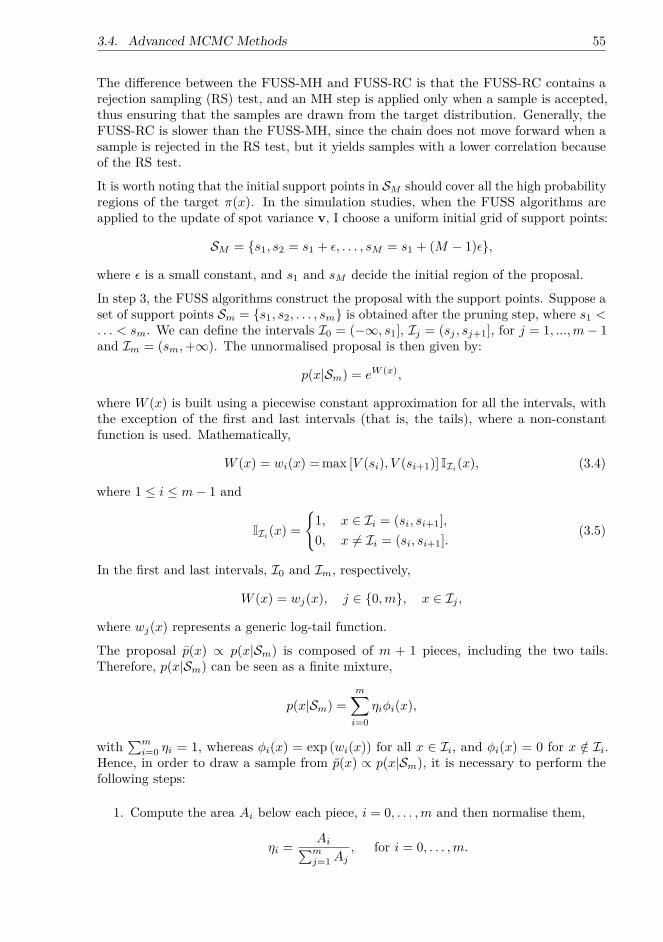
3.4. Advanced MCMC Methods 55
The di�erence between the FUSS-MH and FUSS-RC is that the FUSS-RC contains arejection sampling (RS) test, and an MH step is applied only when a sample is accepted,thus ensuring that the samples are drawn from the target distribution. Generally, theFUSS-RC is slower than the FUSS-MH, since the chain does not move forward when asample is rejected in the RS test, but it yields samples with a lower correlation becauseof the RS test.
It is worth noting that the initial support points in SM
should cover all the high probabilityregions of the target fi(x). In the simulation studies, when the FUSS algorithms areapplied to the update of spot variance v, I choose a uniform initial grid of support points:
SM
= {s
1
, s
2
= s
1
+ ‘, . . . , s
M
= s
1
+ (M ≠ 1)‘},
where ‘ is a small constant, and s
1
and s
M
decide the initial region of the proposal.
In step 3, the FUSS algorithms construct the proposal with the support points. Suppose aset of support points S
m
= {s
1
, s
2
, . . . , s
m
} is obtained after the pruning step, where s
1
<
. . . < s
m
. We can define the intervals I0
= (≠Œ, s
1
], Ij
= (sj
, s
j+1
], for j = 1, ..., m ≠ 1and I
m
= (sm
, +Œ). The unnormalised proposal is then given by:
p(x|Sm
) = e
W (x)
,
where W (x) is built using a piecewise constant approximation for all the intervals, withthe exception of the first and last intervals (that is, the tails), where a non-constantfunction is used. Mathematically,
W (x) = w
i
(x) = max [V (si
), V (si+1
)] IIi(x), (3.4)
where 1 Æ i Æ m ≠ 1 and
IIi(x) =I
1, x œ Ii
= (si
, s
i+1
],0, x ”= I
i
= (si
, s
i+1
].(3.5)
In the first and last intervals, I0
and Im
, respectively,
W (x) = w
j
(x), j œ {0, m}, x œ Ij
,
where w
j
(x) represents a generic log-tail function.
The proposal p(x) Ã p(x|Sm
) is composed of m + 1 pieces, including the two tails.Therefore, p(x|S
m
) can be seen as a finite mixture,
p(x|Sm
) =mÿ
i=0
÷
i
„
i
(x),
withq
m
i=0
÷
i
= 1, whereas „
i
(x) = exp (wi
(x)) for all x œ Ii
, and „
i
(x) = 0 for x /œ Ii
.Hence, in order to draw a sample from p(x) Ã p(x|S
m
), it is necessary to perform thefollowing steps:
1. Compute the area A
i
below each piece, i = 0, . . . , m and then normalise them,
÷
i
= A
iqm
j=1
A
j
, for i = 0, . . . , m.

56Chapter 3. Model Estimation with Advanced MCMC Algorithms:
Simulation Studies
2. Choose a piece (that is, an index j
ú œ {0, . . . , m}) according to the weights ÷
i
fori = 0, . . . , m,
3. Given the index j
ú, draw x
Õ ≥ „
j
ú(x) Ã „
j
ú(x) = exp (wj
ú(x)).
Another issue to address is the pruning step. Martino et al. (2015) propose four di�erentpruning types, and after several tries, I find that the pruning type 4 is the best fit for theproblems considered in this thesis. Considering the length of this thesis, I report only theestimation results obtained by the FUSS algorithms with the pruning type 4. Specifically,the algorithm of the pruning type 4 is as follows:
1. Choose a value ” > 0. Given SM
= {s
1
, ..., s
M
}, set S(0) = SM
, m = M , n = 0, and
L = max1ÆjÆÂ m≠1
2
Ê(s
2j+1
≠ s
2j≠1
)|fi(s2j+1
) ≠ fi(s2j≠1
)|.
2. For r = 1, . . . , R =%
m≠1
2
&:
a) Compute b
r
= (s2r+1
≠ s
2r≠1
)|fi(s2r+1
) ≠ fi(s2r≠1
)|,b) If b
r
Æ ”L, set S(r) = S(r≠1) \ {s
2r
} and n = n + 1,c) Otherwise, if b
r
> ”L, set S(r) = S(r≠1).
3. If n > 0 set n = 0, S(0) = S(R), m = |S(R)| and repeat from step 2.
4. Otherwise, if n = 0, return Sm
= S(R).
3.5 Simulation Studies: Data Generation
In the simulation studies, I estimate three models with di�erent jump structures in thelog price process by all the above Bayesian methods. The input for the estimation is thesimulated one-year log asset prices,1 and considering the computational cost, I followAndrieu et al. (2010) and Martino et al. (2015) and simulate one path2 for each model.Since typically there are 252 trading days a year, I set T = 252, and assume the initial logprice Y
0
and variance v
0
as known, and further assume no jump in the log price at t = 0.
The true values of parameters and initial conditions are reported as follows:
Initial conditions: Y
0
= log(1000), v
0
= 0.02.
Common parameters: Ÿ = 3, ◊ = 0.02, fl = ≠0.8, – = 0.3 in the Heston-0 and Bates-0models and – = 0.1 in the SV-NIG-0 model.3
1I simulate one-year data with 252 observations for two reasons. First, it is computationally economical.Second, for the Bates-0 model with ⁄ = 0.1, with the expected number of jumps per year of approximately25, and for the SV-NIG-0 model with infinite-activity jumps in the log price process, the observations ofjumps are su�cient to estimate the jump-related parameters. This is later justified by the reasonableestimation results of the jump-related parameters in the Bates-0 and SV-NIG-0 models, as shown inTables 3.5 and 3.6.
2In further research, it would be important to simulate more paths and base the algorithm comparisonon more extensive data sets.
3The reason for choosing a smaller – in the SV-NIG-0 is that quite significant volatility has beengenerated by the infinite-activity jumps in the path of the log asset price, and a higher – may make thevariance process and the log price process very volatile with many spiky peaks, and thus too challengingfor the algorithms to estimate the models.

3.5. Simulation Studies: Data Generation 57
0 50 100 150 200 2506.75
6.8
6.85
6.9
6.95
Figure 3.1: Simulated one-year path of the daily log asset price under the Heston-0 model.
0 50 100 150 200 2500
0.005
0.01
0.015
0.02
0.025
0.03
0.035
Figure 3.2: Simulated one-year path of spot variance under the Heston-0 model.
0 50 100 150 200 2505.8
6
6.2
6.4
6.6
6.8
7
7.2
Figure 3.3: Simulated one-year path of the daily log asset price under the Bates-0 model.
Parameters specific to the Bates-0 model: µ
y
= ≠0.05, daily ⁄ = 0.1, ‡
y
= 0.1.
Parameters specific to the SV-NIG-0 model: “ = ≠0.1, ‡ = 0.2, ‹ = 5.
The paths of the daily log asset price and spot variance4 simulated under the Heston-0,Bates, and SV-NIG-0 models are plotted in Figures 3.1–3.6.5
4In the simulation, negative variance processes are discarded.5The set of random numbers is not specified when the paths of the log asset price and variance are
simulated. In future research, it would be interesting to use the same set of random numbers such thatthe simulated paths of variance in all three models are the same.

58Chapter 3. Model Estimation with Advanced MCMC Algorithms:
Simulation Studies
0 50 100 150 200 2500
0.01
0.02
0.03
0.04
0.05
0.06
Figure 3.4: Simulated one-year path of spot variance under the Bates-0 model.
0 50 100 150 200 2506.5
6.6
6.7
6.8
6.9
7
Figure 3.5: Simulated one-year path of the daily log asset price under the SV-NIG-0 model.
0 50 100 150 200 2500.01
0.015
0.02
0.025
0.03
0.035
0.04
Figure 3.6: Simulated one-year path of spot variance under the SV-NIG-0 model.
3.6 Implementation of Algorithms
3.6.1 Likelihood InferenceLet the observations Y = {Y
t
}tØ0
be the log asset price, and let v = {v
t
}tØ0
be theinstantaneous squared volatility of log prices. After the Euler discretisation, under thephysical measure P , I assume that the transition of Y and v is described by the followingstochastic di�erential equations:
Y
t+1
≠ Y
t
=3
µ ≠ 12v
t
4� +
v
t
�‘
Y,t+1
+ J
Y,t+1
,
v
t+1
≠ v
t
= Ÿ(◊ ≠ v
t
)� + –
v
t
�‘
v,t+1
,
(3.6)

3.6. Implementation of Algorithms 59
where � = 1/252, ‘
v,t
, ‘
Y,t
≥ N(0, 1), corr(‘v,t
, ‘
Y,t
) = fl.In the Heston-0 model, J
Y,t
= 0, ’t. The parameters � = {k, ◊, –, fl, µ} are unknown tobe estimated, and v is the latent state variable to be extracted.In the Bates-0 model,
J
Y,t
= ›
Y
t
N
t
, P (Nt
= 1) = ⁄�.
(3.7)
Here the unknown parameter set � = {k, ◊, –, fl, µ, µ
y
, ⁄, ‡
y
}, and v, N and ›
Y are thelatent state variables to be extracted.In the SV-NIG-0 model,
J
Y,t
= “G
Y,t
+ ‡
G
Y,t
‘
JYt
.
(3.8)
Here the unknown parameter set � = {k, ◊, –, fl, µ, “, ‹, ‡}, and v, GY and JY are thelatent state variables to be extracted. ‘
JY ≥ N(0, 1) and is independent of any otherrandom source.In the Hesotn-0 model, the joint posterior is
p(�, v|Y) Ã p(Y, v|�)p(�) (3.9)
ÃT ≠1Ÿ
t=0
1–v
t
�
1 ≠ fl
2
expI
≠‘
2
Y,t+1
≠ 2fl‘
Y,t+1
‘
v,t+1
+ ‘
2
v,t+1
2(1 ≠ fl
2)
Jp(�), (3.10)
where p(�) is the prior of the parameters, and
‘
Y,t
=Y
t
≠ Y
t≠1
≠!µ ≠ 1
2
v
t≠1
"�
v
t≠1
�, (3.11)
‘
v,t
= v
t
≠ v
t≠1
≠ Ÿ(◊ ≠ v
t≠1
)�–
v
t≠1
�. (3.12)
The joint posteriors of the Bates-0 and SV-NIG-0 models can be derived similarly as theHeston-0 model, and the extra likelihoods of jump variables can be computed on thebasis of the model assumptions in Equations 3.7 and 3.8.In the estimation, I cannot directly generate samples from the joint posterior, becauseit is not of a known form. Therefore, I break the joint posterior into conditionals ofparameters and latent state variables, and sample from the conditionals with a Gibbsstep, or the MH and more advanced algorithms, such as the AM and FUSS algorithms,if sampling from one or some of the conditionals is impossible. Alternatively, I use thePMMH to approximate the marginal posterior of parameters or the PGAS to approximatethe joint posterior.Before the estimation, I need to choose appropriate priors for the parameters. I chooseconjugate priors to make the conditional posteriors of known forms if possible. The priorsshould be uninformative so that the posteriors are dominated by the likelihoods.6 The
6The prior is a part of the model specification. If we have strong prior information regarding thedistribution of a parameter, we should use an informative prior for this parameter so that the posterioris not too dispersed and sampling from the posterior would be easier. For example, one may observethat jumps in the path of the log asset price are usually large and negative; then it would be sensibleto assume a normal distribution with negative mean and large variance as the prior for the parametercontrolling the jump size.
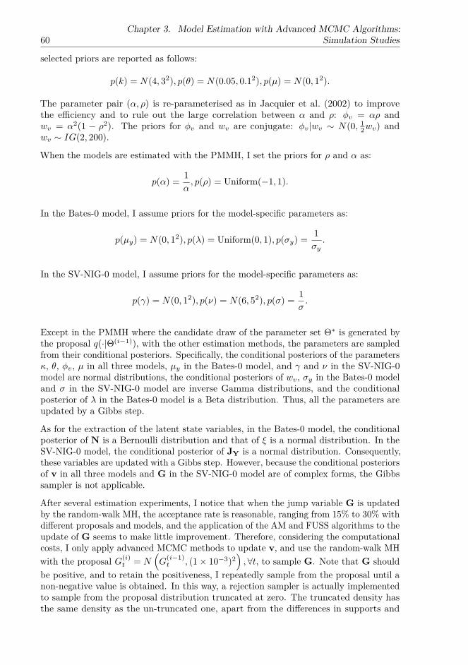
60Chapter 3. Model Estimation with Advanced MCMC Algorithms:
Simulation Studies
selected priors are reported as follows:
p(k) = N(4, 32), p(◊) = N(0.05, 0.12), p(µ) = N(0, 12).
The parameter pair (–, fl) is re-parameterised as in Jacquier et al. (2002) to improvethe e�ciency and to rule out the large correlation between – and fl: „
v
= –fl andw
v
= –
2(1 ≠ fl
2). The priors for „
v
and w
v
are conjugate: „
v
|wv
≥ N(0,
1
2
w
v
) andw
v
≥ IG(2, 200).
When the models are estimated with the PMMH, I set the priors for fl and – as:
p(–) = 1–
, p(fl) = Uniform(≠1, 1).
In the Bates-0 model, I assume priors for the model-specific parameters as:
p(µy
) = N(0, 12), p(⁄) = Uniform(0, 1), p(‡y
) = 1‡
y
.
In the SV-NIG-0 model, I assume priors for the model-specific parameters as:
p(“) = N(0, 12), p(‹) = N(6, 52), p(‡) = 1‡
.
Except in the PMMH where the candidate draw of the parameter set �ú is generated bythe proposal q(·|�(i≠1)), with the other estimation methods, the parameters are sampledfrom their conditional posteriors. Specifically, the conditional posteriors of the parametersŸ, ◊, „
v
, µ in all three models, µ
y
in the Bates-0 model, and “ and ‹ in the SV-NIG-0model are normal distributions, the conditional posteriors of w
v
, ‡
y
in the Bates-0 modeland ‡ in the SV-NIG-0 model are inverse Gamma distributions, and the conditionalposterior of ⁄ in the Bates-0 model is a Beta distribution. Thus, all the parameters areupdated by a Gibbs step.
As for the extraction of the latent state variables, in the Bates-0 model, the conditionalposterior of N is a Bernoulli distribution and that of › is a normal distribution. In theSV-NIG-0 model, the conditional posterior of JY is a normal distribution. Consequently,these variables are updated with a Gibbs step. However, because the conditional posteriorsof v in all three models and G in the SV-NIG-0 model are of complex forms, the Gibbssampler is not applicable.
After several estimation experiments, I notice that when the jump variable G is updatedby the random-walk MH, the acceptance rate is reasonable, ranging from 15% to 30% withdi�erent proposals and models, and the application of the AM and FUSS algorithms to theupdate of G seems to make little improvement. Therefore, considering the computationalcosts, I only apply advanced MCMC methods to update v, and use the random-walk MHwith the proposal G
(i)
t
= N
1G
(i≠1)
t
, (1 ◊ 10≠3)2
2, ’t, to sample G. Note that G should
be positive, and to retain the positiveness, I repeatedly sample from the proposal until anon-negative value is obtained. In this way, a rejection sampler is actually implementedto sample from the proposal distribution truncated at zero. The truncated density hasthe same density as the un-truncated one, apart from the di�erences in supports and

3.6. Implementation of Algorithms 61
normalising constants. When the random-walk MH7 is applied to the update of v, thetrick of repeated sampling is also used to ensure the positiveness of v.
When the AM is applied, I follow the practice in Haario et al. (1999b, 2001) and sets = 2.42 and ‘ = 1 ◊ 10≠4. In particular, instead of adapting the proposal at each MCMCrun, I adapt the proposal at every 100 runs after the initial non-adaptation period of1,000 runs.
When the FUSS algorithms, including the FUSS-RC and FUSS-MH, are applied, I usetype 4 as the pruning scheme and set s
1
= 0.0001, s
M
= 1, �si = s
i+1
≠ s
i
= 0.0001, fori = 1, ..., M ≠ 1, ” = 0.01, and K = 3. The use of the pruning type 4 is motivated bythe findings in Martino et al. (2015) that it is the best pruning type because it selectsthe final set of support points according to a minimax optimality criterion, leading tobetter-quality estimators, a lower correlation between samples, and less computationtime, especially when the target distribution is multimodal with narrow modes. In theestimation, I try all four pruning types and find that the type 4 outperforms the otherpruning types.
In the PF update of the PMMH, I sample the particles {v
i
t
} from v
i
t
= v
Ait≠1
+ Ÿ(◊ ≠
v
Ait≠1
)� + –
Òv
Ait≠1
�‘, where A
i
≥ q
t
(A) Ã w
i
t≠1
and ‘ is a standard normal randomnumber. The particles of the jump variables N and ›
Y in the Bates-0 model and G inthe SV-NIG-0 model are drawn according to model assumptions, and the particles of JYare updated by J
Y,t
= N
t
›
Y
t
, ’t, in the Bates-0 model and by J
Y,t
= “G
t
+Ô
‡G
t
‘
J
, ’t,in the SV-NIG-0 model, where ‘
J is a standard normal random number.
The APF in the PMMH is implemented like the PF in the PMMH. The only di�erence isthat I first sample v
i
t
= v
i
t≠1
+ Ÿ(◊ ≠ v
i
t≠1
)� without the di�usion term and the samplingof index A
i
. Next, I sample the index k
i for v
k
i
t≠1
according to the likelihood of Y
t
conditional on v
i
t
and the weights computed at the previous time step, and then resamplev
k
i
t
according to its tradition density. It is worth mentioning that when the variancevariable v is resampled, the jump variables are associated with k
i, but they are notresampled because of the independence of the jumps.
The implementation of the PF in the PGAS: After the particles at time t have beengenerated, a key step in the PGAS is to sample the ancestor step for the referencetrajectory of v. Specifically, the weights for the ancestor step are computed by:
w
i
t≠1|T Ã w
i
t≠1
1
–
Òv
i
t≠1
exp3
≠ (vN
t
≠ v
i
t
)2
2–
2
v
i
t≠1
�
4(3.13)
Concerning the update of the parameter set in the PMMH, while reading the attacheddiscussion in Andrieu et al. (2010), I noticed an interesting suggestion by ProfessorsMichael Johannes, Nick Polson, and Seung Min Yae that the update step in the PMMHalgorithm can be modified as follows:
Step One: Generate a full vector of latent state variables, X
1:T
, by an SMC update andaccept or reject these draws by a Metropolis update;
7The proposal is a normal distribution with variance 1◊10≠4. It is possible to increase the acceptancerate of v by lowering the variance of the proposal. However, there seems to be a trade-o� betweenthe acceptance rate and the moving speed of the chain. Considering the reasonable value interval of v,1◊10≠4 is quite small as the variance of the proposal, and further reduction of the variance may worsenthe mixing speed of the chain.

62Chapter 3. Model Estimation with Advanced MCMC Algorithms:
Simulation Studies
Step Two: Update the parameters according to p(�|X1:T
, Y
1:T
).
I seek to study the performance of this modified PMMH algorithm combined with thePF as the SMC update in this thesis. In particular, the modified PMMH-PF is labeledPMMH-PF2, and the original version is labeled PMMH-PF1.
Finally, I need to decide the length of the Markov chain as well as the length of the burn-inperiod and the number of particles in the PMCMC methods. Suppose M is the length ofthe Markov chain, M
0
is the length of the burn-in period, and N is the number of particles.After a number of estimation experiments, I observe that when estimating di�erent models,the same algorithm may produce di�erent mixing performance. Therefore, the algorithmicsettings, including M , M
0
, and N , may di�er with di�erent models. The details of thealgorithmic settings are reported in Tables 3.1–3.3. Basically, according to the choiceof M and N , the simulation experiments are divided into two groups: to illustrate theestimation performance with a small number of MCMC iterations and a small particleset, and to obtain a stabilised performance.8
3.7 Results
First of all, it is important to point out that assessing the numerical accuracy of MCMCalgorithms is very di�cult. We use MCMC algorithms because we cannot directly samplefrom the target distribution p(�, X|Y ); instead, we use MCMC algorithms to approximatethe target distribution and examine the performance of algorithms on the basis of theapproximate distribution p(�, X|Y ). For example, in Subsection 3.7.1, I compute theestimation error as the mean squared error of the approximate E(v|Y ) and the simulatedvariance v, and in Subsection 3.7.4, I compare the performance of algorithms in estimatingparameters on the basis of the distance between the approximate E(�|Y ) and the presetparameters �.
However, ideally, the comparison should be based on the distance between the truedistribution and the approximate distribution, that is, E(v|Y ) and E(v|Y ), and E(�|Y )and E(�|Y ). However, we do not know the true distribution; therefore, in this thesis, Ibase the comparison on the approximate distribution, the simulated variance, and presetparameters, following practices in the literature.
3.7.1 Performance of Algorithms with Di�erent Settings:Acceptance Rate, Estimation Error, Log-Likelihood, andComputation Time
Tables 3.1–3.3 report the estimation results of di�erent algorithms with the Heston-0,Bates-0, and SV-NIG-0 models. The results comprise the acceptance rate (AR) of the
8The equilibrium distribution of the Markov chain generated by the MCMC algorithms convergesto the target distribution as the chain length goes to infinity. In this sense, the larger the number ofMCMC iterations (M), the better the performance. However, the improvement brought by increasing Mmay become negligible when M is su�ciently large. Similarly, for the PMCMC methods, increasing Nsignificantly increases the acceptance rate and reduce the estimation error; however, in the simulationtests, I observe that there seems to be an optimal N , after which a further increase of N provides anegligible improvement. In the estimation, I seek to find out the su�ciently large M and N , and refer tothe results as “stabilised results”.
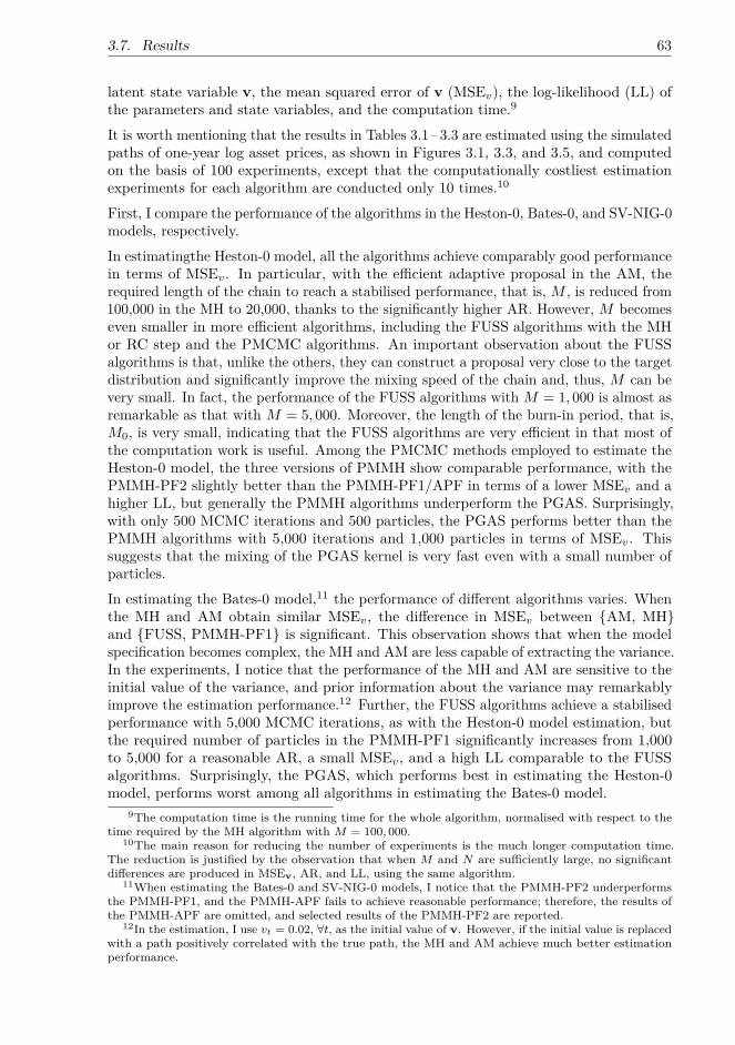
3.7. Results 63
latent state variable v, the mean squared error of v (MSEv
), the log-likelihood (LL) ofthe parameters and state variables, and the computation time.9
It is worth mentioning that the results in Tables 3.1–3.3 are estimated using the simulatedpaths of one-year log asset prices, as shown in Figures 3.1, 3.3, and 3.5, and computedon the basis of 100 experiments, except that the computationally costliest estimationexperiments for each algorithm are conducted only 10 times.10
First, I compare the performance of the algorithms in the Heston-0, Bates-0, and SV-NIG-0models, respectively.In estimatingthe Heston-0 model, all the algorithms achieve comparably good performancein terms of MSE
v
. In particular, with the e�cient adaptive proposal in the AM, therequired length of the chain to reach a stabilised performance, that is, M , is reduced from100,000 in the MH to 20,000, thanks to the significantly higher AR. However, M becomeseven smaller in more e�cient algorithms, including the FUSS algorithms with the MHor RC step and the PMCMC algorithms. An important observation about the FUSSalgorithms is that, unlike the others, they can construct a proposal very close to the targetdistribution and significantly improve the mixing speed of the chain and, thus, M can bevery small. In fact, the performance of the FUSS algorithms with M = 1, 000 is almost asremarkable as that with M = 5, 000. Moreover, the length of the burn-in period, that is,M
0
, is very small, indicating that the FUSS algorithms are very e�cient in that most ofthe computation work is useful. Among the PMCMC methods employed to estimate theHeston-0 model, the three versions of PMMH show comparable performance, with thePMMH-PF2 slightly better than the PMMH-PF1/APF in terms of a lower MSE
v
and ahigher LL, but generally the PMMH algorithms underperform the PGAS. Surprisingly,with only 500 MCMC iterations and 500 particles, the PGAS performs better than thePMMH algorithms with 5,000 iterations and 1,000 particles in terms of MSE
v
. Thissuggests that the mixing of the PGAS kernel is very fast even with a small number ofparticles.In estimating the Bates-0 model,11 the performance of di�erent algorithms varies. Whenthe MH and AM obtain similar MSE
v
, the di�erence in MSEv
between {AM, MH}and {FUSS, PMMH-PF1} is significant. This observation shows that when the modelspecification becomes complex, the MH and AM are less capable of extracting the variance.In the experiments, I notice that the performance of the MH and AM are sensitive to theinitial value of the variance, and prior information about the variance may remarkablyimprove the estimation performance.12 Further, the FUSS algorithms achieve a stabilisedperformance with 5,000 MCMC iterations, as with the Heston-0 model estimation, butthe required number of particles in the PMMH-PF1 significantly increases from 1,000to 5,000 for a reasonable AR, a small MSE
v
, and a high LL comparable to the FUSSalgorithms. Surprisingly, the PGAS, which performs best in estimating the Heston-0model, performs worst among all algorithms in estimating the Bates-0 model.
9The computation time is the running time for the whole algorithm, normalised with respect to thetime required by the MH algorithm with M = 100, 000.
10The main reason for reducing the number of experiments is the much longer computation time.The reduction is justified by the observation that when M and N are su�ciently large, no significantdi�erences are produced in MSEv, AR, and LL, using the same algorithm.
11When estimating the Bates-0 and SV-NIG-0 models, I notice that the PMMH-PF2 underperformsthe PMMH-PF1, and the PMMH-APF fails to achieve reasonable performance; therefore, the results ofthe PMMH-APF are omitted, and selected results of the PMMH-PF2 are reported.
12In the estimation, I use vt = 0.02, ’t, as the initial value of v. However, if the initial value is replacedwith a path positively correlated with the true path, the MH and AM achieve much better estimationperformance.
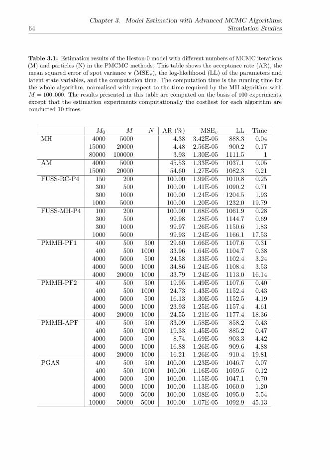
64Chapter 3. Model Estimation with Advanced MCMC Algorithms:
Simulation Studies
Table 3.1: Estimation results of the Heston-0 model with di�erent numbers of MCMC iterations(M) and particles (N) in the PMCMC methods. This table shows the acceptance rate (AR), themean squared error of spot variance v (MSEv), the log-likelihood (LL) of the parameters andlatent state variables, and the computation time. The computation time is the running time forthe whole algorithm, normalised with respect to the time required by the MH algorithm withM = 100, 000. The results presented in this table are computed on the basis of 100 experiments,except that the estimation experiments computationally the costliest for each algorithm areconducted 10 times.
M
0
M N AR (%) MSEv
LL TimeMH 4000 5000 4.38 3.42E-05 888.3 0.04
15000 20000 4.48 2.56E-05 900.2 0.1780000 100000 3.93 1.30E-05 1111.5 1
AM 4000 5000 45.53 1.33E-05 1037.1 0.0515000 20000 54.60 1.27E-05 1082.3 0.21
FUSS-RC-P4 150 200 100.00 1.99E-05 1010.8 0.25300 500 100.00 1.41E-05 1090.2 0.71300 1000 100.00 1.24E-05 1204.5 1.93
1000 5000 100.00 1.20E-05 1232.0 19.79FUSS-MH-P4 100 200 100.00 1.68E-05 1061.9 0.28
300 500 99.98 1.28E-05 1144.7 0.69300 1000 99.97 1.26E-05 1150.6 1.83
1000 5000 99.93 1.24E-05 1166.1 17.53PMMH-PF1 400 500 500 29.60 1.66E-05 1107.6 0.31
400 500 1000 33.96 1.64E-05 1104.7 0.384000 5000 500 24.58 1.33E-05 1102.4 3.244000 5000 1000 34.86 1.24E-05 1108.4 3.534000 20000 1000 33.79 1.24E-05 1113.0 16.14
PMMH-PF2 400 500 500 19.95 1.49E-05 1107.6 0.40400 500 1000 24.73 1.43E-05 1152.4 0.43
4000 5000 500 16.13 1.30E-05 1152.5 4.194000 5000 1000 23.93 1.25E-05 1157.4 4.614000 20000 1000 24.55 1.21E-05 1177.4 18.36
PMMH-APF 400 500 500 33.09 1.58E-05 858.2 0.43400 500 1000 19.33 1.45E-05 885.2 0.47
4000 5000 500 8.74 1.69E-05 903.3 4.424000 5000 1000 16.88 1.26E-05 909.6 4.884000 20000 1000 16.21 1.26E-05 910.4 19.81
PGAS 400 500 500 100.00 1.23E-05 1046.7 0.07400 500 1000 100.00 1.16E-05 1059.5 0.12
4000 5000 500 100.00 1.15E-05 1047.1 0.704000 5000 1000 100.00 1.13E-05 1060.0 1.204000 5000 5000 100.00 1.08E-05 1095.0 5.54
10000 50000 5000 100.00 1.07E-05 1092.9 45.13

3.7. Results 65
Table 3.2: Estimation results of the Bates-0 model with di�erent numbers of MCMC iterations(M) and particles (N) in the PMCMC methods. This table shows the acceptance rate (AR), themean squared error of spot variance v (MSEv), the log-likelihood (LL) of the parameters andlatent state variables, and the computation time. The computation time is the running time forthe whole algorithm, normalised with respect to the time required by the MH algorithm withM = 100, 000. The results presented in this table are computed on the basis of 100 experiments,except that the estimation experiments computationally the costliest for each algorithm areconducted 10 times.
M
0
M N AR(%) MSEv
LL TimeMH 4000 5000 11.62 4.24E-05 975.7 0.05
15000 20000 7.72 4.04E-05 1033.9 0.2280000 100000 8.54 2.59E-05 1055.9 1
AM 4000 5000 66.60 8.91E-05 1050.2 0.0715000 20000 64.16 2.61E-05 1107.5 0.30
FUSS-RC-P4 150 200 99.88 7.39E-05 1015.1 0.21300 500 99.95 4.68E-05 1066.5 0.40300 1000 99.98 2.46E-05 1170.7 0.98
1000 5000 99.98 1.62E-05 1192.2 10.24FUSS-MH-P4 150 200 100.00 4.32E-05 1015.0 0.17
300 500 99.96 4.42E-05 1062.6 0.45300 1000 99.80 1.96E-05 1113.1 1.18
1000 5000 100.00 1.87E-05 1123.4 10.13PMMH-PF1 400 500 500 5.27 5.14E-05 956.3 0.24
400 500 1000 5.47 4.29E-05 1042.5 0.31400 500 5000 15.30 2.50E-05 1064.2 0.55
4000 5000 500 1.27 5.35E-05 1015.6 0.434000 5000 1000 1.56 2.39E-05 1031.8 0.654000 5000 5000 21.24 1.89E-05 1152.3 2.40
PMMH-PF2 4000 5000 1000 1.10 2.70E-05 962.8 0.67PGAS 4000 5000 500 97.28 7.43E-05 1067.8 0.55
4000 5000 1000 98.16 6.19E-05 1078.5 0.924000 5000 5000 99.34 3.43E-05 1088.5 3.734000 20000 5000 98.29 3.46E-05 1091.4 14.00

66Chapter 3. Model Estimation with Advanced MCMC Algorithms:
Simulation Studies
Table 3.3: Estimation results of the SV-NIG-0 model with di�erent numbers of MCMC iterations(M) and particles (N) in the PMCMC methods. This table shows the acceptance rate (AR), themean squared error of spot variance v (MSEv), the log-likelihood (LL) of the parameters andlatent state variables, and the computation time. The computation time is the running time forthe whole algorithm, normalised with respect to the time required by the MH algorithm withM = 100, 000. The results presented in this table are computed on the basis of 100 experiments,except that the estimation experiments computationally the costliest for each algorithm areconducted 10 times.
M0 M N AR (%) MSEv
LL TimeMH 4000 5000 12.82 2.12E-05 927.02 0.05
15000 20000 11.82 1.87E-05 942.82 0.2780000 100000 37.91 1.77E-05 1017.70 1
AM 4000 5000 33.22 2.19E-05 922.88 0.1415000 20000 56.07 1.58E-05 953.88 0.6940000 50000 56.94 1.55E-05 966.95 2.71
FUSS-RC-P4 150 200 100.00 2.61E-05 898.86 0.12300 500 100.00 2.17E-05 918.43 0.32300 1000 100.00 2.20E-05 926.36 0.89
1000 5000 100.00 1.15E-05 955.64 10.353000 10000 100.00 8.31E-06 1022.5 33.79
FUSS-MH-P4 150 200 100.00 2.46E-05 974.94 0.12300 500 100.00 2.14E-05 979.08 0.34300 1000 100.00 1.63E-05 938.97 0.87
1000 5000 100.00 1.46E-05 983.45 10.243000 10000 100.00 1.31E-05 991.81 33.71
PMMH-PF1 400 500 500 35.30 1.97E-05 963.23 0.36400 500 1000 49.86 1.47E-05 1020.15 0.39
4000 5000 500 36.01 1.14E-05 1006.39 3.564000 5000 1000 45.37 9.00E-06 1019.26 3.66
10000 20000 1000 50.20 7.63E-06 1026.49 11.77PMMH-PF2 4000 5000 1000 46.42 1.21E-05 1002.80 3.00
10000 20000 1000 58.60 1.19E-05 1001.20 13.83PGAS 400 500 500 98.67 2.25E-05 998.84 0.06
400 500 1000 98.84 1.31E-05 1008.69 0.094000 5000 500 99.50 2.15E-05 997.45 0.504000 5000 1000 99.71 6.53E-06 1013.50 0.744000 5000 5000 99.86 1.01E-05 998.49 3.09
10000 20000 1000 99.80 6.24E-06 1027.51 1.67

3.7. Results 67
According to the estimation results of the SV-NIG-0 model, the MSEv
of the MH isthe largest; however, the LL obtained by the MH ranks the fourth highest, implyingan estimation result more consistent with the data than the AM with 20,000 MCMCiterations. To investigate, I increase M for the AM to 50,000; however, its performance iscomparable to that with M = 20, 000. The FUSS algorithms significantly outperformthe MH and AM, but with a more complex model specification, the optimal M for theFUSS algorithms significantly increases. Furthermore, even with the optimal M , theFUSS algorithms still slightly underperform the PMMH-PF1 and PGAS, the latter beingthe best algorithm again in estimating the SV-NIG-0 model, as with the Heston-0 modelestimation.
Moreover, the computation times of di�erent algorithms in estimating the Heston-0, Bates-0, and SV-NIG-0 models are reported in Tables 3.1–3.3. In each table, the computationtime is normalised with respect to the time required by the MH with M = 100, 000.Generally, the computation time increases proportionally to the increase of M , whereasit changes more slowly than the increase of N in the PMCMC methods. As expected,with a fixed M , the MH is the fastest, the AM ranks the second fastest, followed by thePMCMC methods, and the FUSS algorithms are the slowest. In particular, the FUSS-RCis slightly slower than the FUSS-MH owing to the RS test in the FUSS-RC, and thecomputation time of the PGAS is only about 30% of that of the PMMH algorithms withthe same M and N . However, if we focus on achieving comparable estimation results, inestimating the Heston-0 and Bates-0 models, the FUSS algorithms are more e�cient thanthe others; however, the advantage of the FUSS algorithms over the AM and MH becomessmaller when estimating the complicated SV-NIG-0 model. Furthermore, although itsperformance is poor in estimating the Bates-0 model, the PMMH-PF1 is very competitivein estimating the SV-NIG-0 model. Specifically, the PMMH-PF1 takes about 40% of thecomputation time of the MH to outperform the MH and the AM, and about 30% of thecomputation time of the FUSS-RC to beat the FUSS-RC. More importantly, the PGASis extremely e�cient in estimating the SV-NIG-0 model, because it only takes 74% of thecomputation time of the MH to beat all the other algorithms.
Next, I analyse how di�erent jump structures a�ect the estimation performance.
First, I discuss how jump structures change the AR. The ARs of the MH in estimatingthe Heston-0 and Bates-0 models are very low; however, the AR becomes reasonable inestimating the SV-NIG-0 model. The ARs of the AM, FUSS, and PGAS algorithms arestable with di�erent models. For the Bates-0 model, the AR of the PMMH-PF1 is verylow.13 A possible reason for the low AR of the PMMH-PF1 in estimating the Bates-0model is that, although the simulated compound Poisson jumps are rare events, theirjump sizes are significant; therefore, in the estimation, they play an important role incomputing likelihoods and in deciding the weights of the particles. However, since I haveno prior information of the jumps, and since the jump times and sizes are independentof each other, the particles generated for the jumps are highly random. Therefore, onlyparticles with “correct” jump times and sizes are assigned reasonable weights and mostof the generated particles are actually useless, which largely a�ects the performanceof the SMC update. On the other side, in the SV-NIG-0 model with infinite-activityjumps, where the jumps are on average less significant and, therefore, less distinguishable
13In the estimation, I use the random-walk normal distribution with a diagonal covariance matrixas the proposal. I have also tried to use other covariance matrices by running the estimation for someiterations, computing the covariance of the parameters, and setting the covariance matrix as the proposalcovariance matrix. However, this step produces negligible improvement.

68Chapter 3. Model Estimation with Advanced MCMC Algorithms:
Simulation Studies
from di�usions, even if the particles of the jumps are unrealistic, they may be assignedreasonable weights, because “wrong jumps” can be o�set by di�usions. In other words,the impact of the jumps in the SV-NIG-0 model on the weights of the particles is lesssignificant than that of the compound Poisson jumps in the Bates-0 model.Another observation is that when the performance of the MH, AM, FUSS-RC, andFUSS-MH is stable across di�erent models, the performance of the PMCMC algorithmsseems mixed:1. Comparison of the PMMH-PF1 and the PMMH-PF2.When estimating the Heston-0 model, the PMMH-PF1 yields a poorer performance thanthe PMMH-PF2, which is plausible because the samples of the parameters in the latterare updated on the basis of the updated variance and data. However, when estimating theBates-0 and SV-NIG-0 models, the PMMH-PF2 underperforms the PMMH-PF1. In fact,in the simulation studies, I observe that the performance of all the PMCMC methods isvery sensitive to the parameter –, because it is important in generating particles of v,and with a higher –, the particles of v may vary significantly. Further, the particles ofthe jumps may be quite varied as well, especially for the Bates-0 model, and compared tothe Heston-0 model without jumps, jumps in the Bates-0 model and SV-NIG-0 modelplay a relatively important role in the likelihoods. Therefore, fewer particles are neededto create a diverse combination of jumps and variance v with a higher –. However, ahigher – may not be consistent with the data, and the PMMH-PF2 seems to producea less significant – than the PMMH-PF1, as confirmed by the estimation results of theparameters in the Heston-0 model.2. Comparison of the PF and the APF used in the PMMH.When estimating the Heston-0 model, the PMMH-APF obtains an estimation performancecomparable to that of the PMMH-PF1/PF2; however, when estimating the other twomodels, its estimation performance is rather poor. The reason for the failure of the APFto estimate the Bates-0 and SV-NIG-0 models is the inclusion of independent jumps,which makes the advantage of the APF become a handicap. The key idea of the APFdoes not work for models with independent random sources. In the estimation with thePMMH-APF, I first predict the variance at current time t on the basis of the particlesof variance at t ≠ 1 without the random di�usion term, and simulate the particles ofthe jumps without any prior information, and then choose the most likely particles ofvariance at t ≠ 1 according to the likelihood of the observation at time t and weights att ≠ 1. Second, I re-predict the variance at t with the random di�usion term, and choosethe simulated jumps with the indices of the selected particles, rather than re-simulatingthe jumps, because the jumps are independent of the past track and re-simulating themmay a�ect the e�ect of auxiliary variables. Therefore, the independence of the jumpsreduces the e�ectiveness of the APF.3. Comparison of the PMMH and the PGAS.Although the PGAS is very similar in design to the PMMH-PF2, they di�er in the stepof updating particles of the variance and jumps. In the estimation using the PMMH-PF2,I use the PF to generate the particles, whereas in the PGAS, the update of particlesuses some prior information embodied in the reference trajectory. In addition, unlike thePG sampler, after each time step in the SMC update, a new trajectory is obtained byan ancestor sampling step, which connects part of the reference trajectory, X
Õt:T
, withone of the generated particle trajectories, X
i
1:t≠1
, i œ {1, ..., N}, with probabilities givenby their importance weights. As pointed out in Lindsten et al. (2014), the PGAS is

3.7. Results 69
0 50 100 150 200 250-0.25
-0.2
-0.15
-0.1
-0.05
0
0.05
0.1
0.15
0.2
diffusion in the return
compound Poisson jumps
Figure 3.7: Randomness sources in the Bates-0 model.
particularly competitive in extracting a high-dimensional and highly autocorrelated statetrajectory. This is confirmed by the superior estimation results of the PGAS in estimatingthe Heston-0 and SV-NIG-0 models, and its performance with only a small number ofMCMC iterations and a small set of particles is better than the other algorithms with alarge number of MCMC iterations and particles.
Indeed, there is a remarkable di�erence between the PMMH and PGAS, although bothbelong to the PMCMC methods. In particular, just as the PMMH algorithm canbe regarded an approximation of the ideal marginal MH sampler targeting p(�|Y
1:T
),the PGAS can be regarded an approximation of the ideal Gibbs sampler targetingp(�, X
1:T
|Y1:T
). Therefore, as pointed out in Lindsten et al. (2014), the respectiveperformances of the PMMH and PGAS depend on the properties of the marginal MHsampler and Gibbs sampler and, therefore, depend heavily on the properties of specificproblems. For the Heston-0 and SV-NIG-0 models, the ideal Gibbs sampler seems tohave better mixing properties than the marginal MH sampler.
4. Comparison of the PMCMC methods and other MCMC methods.
Generally, compared to the MH, the use of adaptive proposals in the AM can significantlyraise the AR, thus reducing M to achieve a stabilised performance. However, as themodel specification becomes complex, the MH and AM underperform the algorithms thatare able to deal with a complicated target distribution and strong dependence betweenparameters and state variables. In particular, when estimating all three models, theFUSS-RC outperforms the FUSS-MH, because of the RS step in the FUSS-RC.
Although the PMCMC methods achieve comparably good estimation performance as theFUSS algorithms in estimating the Heston-0, their performance deteriorates in estimatingthe Bates-0 model with rare large jumps included, even when the number of particlesand length of the chain are quite large. However, the PMCMC algorithms beat theothers in estimating the SV-NIG-0 model. The reason is the di�erent features of the

70Chapter 3. Model Estimation with Advanced MCMC Algorithms:
Simulation Studies
0 50 100 150 200 250-0.04
-0.03
-0.02
-0.01
0
0.01
0.02
0.03
0.04
diffusion in the return
NIG jumps
Figure 3.8: Randomness sources in the SV-NIG-0 model.
jumps in the Bates-0 and SV-NIG-0 models. The simulated compound Poisson jumps arediscrete jumps, and their expected mean size and variance are large, with µ
y
= ≠0.05and ‡
y
= 0.1; therefore, the compound Poisson jumps bring on large changes in thelog prices, which are relatively easy to identify. Since there is a distinctive di�erencebetween the simulated compound Poisson jumps and simulated di�usion terms, as shownin Figure 3.7, the algorithms can easily classify the di�erent sources of randomness createdby the jumps and di�usions. However, for the model with NIG jumps, the expectedmean of jumps is “/‹ = ≠0.02, and as shown in Figure 3.8 of the simulated NIG jumpsagainst the simulated di�usions, large jumps are less significant than those created bythe Bates-0 model. When estimating the SV-NIG-0 model, the algorithms may mix therandomness created by the infinite-activity jumps and di�usions, especially for the smallfrequent jumps. Since the NIG jumps are not significant compared to the compoundPoisson jumps, their role in the likelihoods and importance weights of particles is lessimportant than that of the compound Poisson jumps. In other words, even if the jumpsare not correctly identified, the extra randomness can be captured by the di�usion terms,which explains the higher AR and the better mixing of the chain in the estimation of theSV-NIG-0 model than the Bates-0 model.
Overall, the strength of the PMMH algorithms, compared to the other MCMC methods, isthat they simultaneously update the parameters and state variables, targeting p(�|Y
1:T
),and the PGAS simultaneously update all the variables, targeting p(�, X
1:T
|Y1:T
), whichis very important in the presence of a strong dependence between state variables andparameters. In the Bates-0 model, the independent rare large events reduce the e�ciencyof the PMCMC methods; however, in the SV-NIG-0 model, where the jumps are hardto distinguish from the di�usions and their role in deciding the weights of the particlesis relatively small, most particles generated by the PMCMC methods are useful and,therefore, the PMCMC beat the other algorithms and are very competitive in this case.

3.7. Results 71
3.7.2 VarianceIn this subsection, I analyse the extraction of variance in the Heston-0, Bates-0, andSV-NIG-0 models. The figures of the extracted variance against the simulated path arelisted in Appendix A.
The figures show that the MH and AM yield relatively poor results when little priorinformation of variance is available. Specifically, given that the initial variance is v
t
= 0.02,’t = 1, ..., 252, the MH and AM do not achieve the true variance dynamics and are sensitiveto the initial flat values, whereas the other algorithms capture the variance dynamicsrelatively well. Moreover, I observe that when estimating all three models, the FUSS andPMCMC algorithms tend to extract a path of variance more volatile than the true one.In particular, in the Bates-0 model, the path extracted by the PMMH-PF1 is the mostvolatile: it captures the concaveness that occurs between 50 and 100, which the otheralgorithms miss. In the SV-NIG-0 model, the di�erences between the paths of varianceextracted by the MH, AM, and FUSS algorithms are much less significant, and clearlythe PMCMC methods achieve better performance in generating more volatility and moreconsistent levels for the paths.
The extraction of the path of variance is relevant to values of Ÿ and –. The paths ofvariance extracted by the FUSS and PMCMC algorithms are more volatile than those bythe MH and AM algorithms, and correspondingly, Ÿ and – estimated by the FUSS andPMCMC are more significant than those by the MH and AM. In fact, in the estimationwith the PMCMC methods, the update of variance is very sensitive to –. Specifically, amore significant – can introduce more diversity to the particle set of variance; therefore, itmay prevent the particles from accumulating in a local region and increase the e�ciencyof the SMC update.
3.7.3 JumpsThe figures of the extracted jumps against the simulated jumps are listed in Appendix B.In the Bates-0 model, all the algorithms extract the discrete rare large jumps quite well interms of estimating both jump times and jump sizes. However, extracting infinite-activityNIG jumps is much more di�cult than extracting discrete finite-activity compoundPoisson jumps. Overall, the extracted NIG jumps are smaller than the true jumps,especially the downside jumps and jumps extracted by the FUSS and PMMH. Interesting,although the extraction of NIG jumps is not as accurate as that of compound Poissonjumps, there are significant similarities in the extracted NIG jumps across di�erentalgorithms, suggesting that the MCMC methods tend to reallocate the randomnesscreated by Brownian di�usions and infinite-activity jumps, especially the frequent smalljumps.
3.7.4 Parameter EstimationFirst, I analyse the parameter estimation results of the Heston-0 model as shown inTable 3.4. The MH and AM produce similar parameter estimation results, except thatŸ and – are more significant with the AM. Further, Ÿ and – become higher with theFUSS algorithms and are highest with the PMMH and PGAS. A possible reason for thesignificant Ÿ and – with some algorithms is that they tend to extract a volatile pathof variance with more spiky peaks and valleys, and this may a�ect the values of theparameters that are key in creating the changes in the path of variance.

72Chapter 3. Model Estimation with Advanced MCMC Algorithms:
Simulation StudiesTable 3.4: Parameter estimates of the Heston-0 model using simulated one-year data of dailylog asset prices. The parameter values are the mean of the posteriors as annual decimals. Thestandard errors are the standard deviations of the posteriors, reported in parentheses.
True values MH AM FUSS-RC-P4 FUSS-MH-P4M
0
80000 15000 1000 1000M 100000 20000 5000 5000Ÿ 3 2.536 2.562 2.615 3.240
(1.895) (1.799) (1.705) (1.860)◊ 0.02 0.022 0.023 0.016 0.018
(0.025) (0.025) (0.009) (0.008)– 0.3 0.147 0.156 0.186 0.171
(0.031) (0.013) (0.035) (0.025)fl -0.8 -0.849 -0.840 -0.790 -0.731
(0.091) (0.064) (0.098) (0.202)µ -0.1 -0.151 -0.152 -0.142 -0.136
(0.104) (0.105) (0.096) (0.100)
True values PMMH-PF1 PMMH-PF2 PMMH-APF PGASM
0
4000 4000 4000 10000M 20000 20000 5000 50000N 1000 1000 1000 5000Ÿ 3 2.895 2.730 2.662 3.180
(0.649) (1.561) (0.421) (1.881)◊ 0.02 0.021 0.017 0.016 0.019
(0.005) (0.008) (0.001) (0.009)– 0.3 0.251 0.139 0.469 0.199
(0.067) (0.043) (0.033) (0.052)fl -0.8 -0.825 -0.874 -0.701 -0.804
(0.076) (0.072) (0.003) (0.069)µ -0.1 -0.186 -0.161 -0.163 -0.152
(0.071) (0.092) (0.037) (0.095)
Further, in the Heston-0 model, all the algorithms estimate µ more negative than itstrue value. This may also be explained by the extracted path of variance being flatterthan the true path. As captured by the correlation parameter fl, a strong negativecorrelation occurs between the changes in variance and log asset prices, and when thespot variance increases, the log price process tends to drop. However, when the peaks inthe true path of variance are not captured by the algorithms, the extracted variance isless capable of causing a drop with “enough” magnitude in the log asset price, which hasto be compensated for by a µ more negative than its true value.
According to the estimation results of the Bates-0 and SV-NIG-0 models as shown inTables 3.5 and 3.6, the values of Ÿ and – are also correlated with the performance ofalgorithms in extracting variance, and overall, – is higher with the PMCMC methods.This suggests a potential problem of the PMMH. In the estimation with the PMMH, I usean SMC algorithm to update the latent state variable v. In particular, I generate a set ofparticles of the variance v according to its transition kernel: v
t
= v
t≠1
+ Ÿ(◊ ≠ v
t≠1
)� +
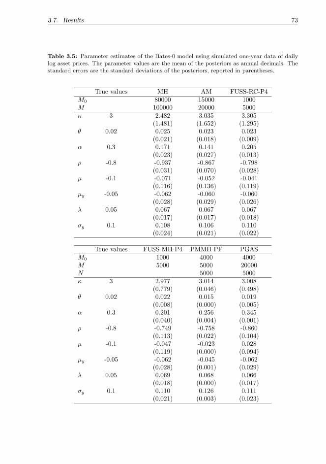
3.7. Results 73
Table 3.5: Parameter estimates of the Bates-0 model using simulated one-year data of dailylog asset prices. The parameter values are the mean of the posteriors as annual decimals. Thestandard errors are the standard deviations of the posteriors, reported in parentheses.
True values MH AM FUSS-RC-P4M
0
80000 15000 1000M 100000 20000 5000Ÿ 3 2.482 3.035 3.305
(1.481) (1.652) (1.295)◊ 0.02 0.025 0.023 0.023
(0.021) (0.018) (0.009)– 0.3 0.171 0.141 0.205
(0.023) (0.027) (0.013)fl -0.8 -0.937 -0.867 -0.798
(0.031) (0.070) (0.028)µ -0.1 -0.071 -0.052 -0.041
(0.116) (0.136) (0.119)µ
y
-0.05 -0.062 -0.060 -0.060(0.028) (0.029) (0.026)
⁄ 0.05 0.067 0.067 0.067(0.017) (0.017) (0.018)
‡
y
0.1 0.108 0.106 0.110(0.024) (0.021) (0.022)
True values FUSS-MH-P4 PMMH-PF PGASM
0
1000 4000 4000M 5000 5000 20000N 5000 5000Ÿ 3 2.977 3.014 3.008
(0.779) (0.046) (0.498)◊ 0.02 0.022 0.015 0.019
(0.008) (0.000) (0.005)– 0.3 0.201 0.256 0.345
(0.040) (0.004) (0.001)fl -0.8 -0.749 -0.758 -0.860
(0.113) (0.022) (0.104)µ -0.1 -0.047 -0.023 0.028
(0.119) (0.000) (0.094)µ
y
-0.05 -0.062 -0.045 -0.062(0.028) (0.001) (0.029)
⁄ 0.05 0.069 0.068 0.066(0.018) (0.000) (0.017)
‡
y
0.1 0.110 0.126 0.111(0.021) (0.003) (0.023)

74Chapter 3. Model Estimation with Advanced MCMC Algorithms:
Simulation Studies
Table 3.6: Parameter estimates of the SV-NIG-0 model using simulated one-year data of dailylog asset prices. The parameter values are the mean of the posteriors as annual decimals. Thestandard errors are the standard deviations of the posteriors, reported in parentheses.
True values MH AM FUSS-RC-P4M
0
80000 40000 3000M 100000 50000 10000Ÿ 3 3.293 2.828 3.062
(2.093) (1.584) (2.024)◊ 0.02 0.024 0.021 0.022
(0.009) (0.005) (0.008)– 0.1 0.088 0.095 0.080
(0.011) (0.020) (0.012)fl -0.8 -0.805 -0.844 -0.790
(0.063) (0.070) (0.070)µ -0.1 -0.211 -0.139 -0.191
(0.037) (0.061) (0.055)“ -0.1 -0.122 -0.088 -0.156
(0.072) (0.116) (0.167)‹ 5 8.693 8.457 5.900
(3.353) (3.422) (1.406)‡ 0.2 0.254 0.253 0.265
(0.058) (0.055) (0.054)
True values FUSS-MH-P4 PMMH-PF1 PGASM
0
3000 10000 10000M 10000 20000 20000N 1000 1000Ÿ 3 3.160 3.615 3.162
(1.786) (1.788) (1.826)◊ 0.02 0.020 0.019 0.027
(0.006) (0.004) (0.008)– 0.3 0.088 0.131 0.095
(0.010) (0.048) (0.037)fl -0.8 -0.849 -0.826 -0.814
(0.072) (0.086) (0.076)µ -0.1 -0.131 -0.132 -0.307
(0.038) (0.050) (0.127)“ -0.1 -0.078 -0.098 -0.088
(0.071) (0.031) (0.195)‹ 5 5.974 5.218 5.567
(1.513) (1.145) (1.418)‡ 0.2 0.252 0.137 0.244
(0.055) (0.083) (0.058)

3.7. Results 75
–
v
t≠1
�‘, where ‘ is a standard normal random number. The transition kernel showsthat the diversity of the particle set is determined by the parameter –; therefore, a larger– is more likely to produce a particle set that better represents the target distribution.In other words, – has an important role in the performance of the SMC update in that itnot only directly a�ects the likelihood as a parameter involved in the likelihood function,but also indirectly changes it by generating a particle set. Thus, it is not surprising that alarger – is more likely to be accepted with the PMMH-PF1, whereas with the PGAS andPMMH-PF2, – is updated according to its conditional posterior as in the MH, AM, andFUSS, and whether it is accepted or not is not related to the likelihood of the particle set.
In the Bates-0 model, all the algorithms succeed in estimating the jump-related parametersµ
y
, ⁄, and ‡
y
, owing to very accurate extraction of the jumps. However, in the SV-NIG-0model, the jump-related parameters, including “, ‹, and ‡, are harder to identify fromthe data. Specifically, the expected mean size of the NIG jumps is “/‹, and the varianceof the NIG jumps is ‹‡
2 + “
2
/‹
3. When the estimated values are similar in the otheralgorithms, “ is more negative with the FUSS-RC, and ‡ is lower in the PMMH-PF1.Correspondingly, the NIG jumps extracted by the FUSS-RC show downside jumps thatare more negative, and the jumps extracted by the PMMH-PF1 are less significant thanthose extracted by the other algorithms. Moreover, the arrival rate of the NIG jumps is:
fi
NIG
(dx) = ‡–
fi
e
—x
K
1
(–|x|)|x| dx, (3.14)
where – = ‹
2
/‡
2 + “
2
/‡
4, — = “/‡
2, and K
1
is the modified Bessel function of the thirdkind with index 1. Therefore, generally, a more significant ‹ with the MH and AM leadsto a higher arrival rate, and as reflected in the figures of extracted jumps, there are morefrequent small jumps extracted by the MH and AM.
Further, in the SV-NIG-0 model, the values of µ with all algorithms are more negative thanits true value. Indeed, this result may come from the less significant jumps. Compared tothe simulated NIG jumps, the number of the extracted jumps are fewer, the jump sizesare smaller, and, markedly, the algorithms miss several large downside jumps.

76Chapter 3. Model Estimation with Advanced MCMC Algorithms:
Simulation Studies
3.8 Discussion
In this chapter, I compare the estimation performance of advanced MCMC algorithmscomprising the AM (Haario et al., 1999a, 2001), the FUSS algorithms (Martino et al.,2015), and the PMCMC methods against conventional MH algorithms (Hastings, 1970;Metropolis et al., 1953). The PMCMC methods comprise the PMMH-PF1/PF2/APF(Andrieu et al., 2010) and the PGAS (Lindsten et al., 2014). The comparison is based onsimulation studies. In particular, I examine, from simulated data, how these algorithmsperform in estimating the a�ne Heston-0, Bates-0, and SV-NIG-0 models with di�erentjump structures and in dealing with the problems of high dimensions, complicated targetdistributions, and strong dependence between latent state variables and parameters.While some finance research applies the conventional MCMC or SMC algorithms toestimate stochastic volatility models with jumps (see, for example, Christo�ersen et al.,2010a; Eraker et al., 2003; Kaeck and Alexander, 2013a), few attempts have been made toapply the above algorithms. This chapter seek to examine how the advanced estimationmethods perform in estimating complicated financial models compared to conventionalMH algorithms.
The results of the simulation studies show that di�erent jump structures significantlya�ect the estimation performance of the algorithms. In particular, when all the algorithmsperfectly extract the compound Poisson jumps in the Bates-0 model, they fail to distinguishthe randomness created by the infinite-activity NIG jumps and Brownian di�usions inthe log price process of the SV-NIG-0 model. This makes parameter estimation andvariance extraction very challenging, and the extra complexity brought on by the NIGjumps requires the FUSS and PMCMC methods to increase the numbers of MCMC runsand particles, while the MH and AM are less capable of dealing with complicated modelspecifications. In contrast, compound Poisson jumps create rare but significant changesin the path of the log price process, which are distinctive of di�usions. Therefore, inthe PMCMC methods, jumps in log asset prices play an important role in deciding theimportance weights of particles. The results of the simulation studies show that in theestimation of the Bates-0 model, the acceptance rate of the PMCMC methods significantlydecreases, and the e�ciency drops. However, the other algorithms are less vulnerableto the specification of compound Poisson jumps and achieve consistent performance indi�erent models.
Considering the complexity and computational costs of di�erent algorithms, I concludethat for models with a simple specification, the MH is very competitive because of its lowcomputational cost. However, if the target distribution is complicated or the proposalof the MH is inappropriate, the acceptance rate may be very low, and most generateddraws are wasted. The AM makes use of the previous samples and dynamically tunes theproposal, and this online-tuned adaptive proposal can significantly raise the acceptancerate and speed up the convergence of the chain.
Moreover, when there is a strong correlation between state variables and the targetdistribution becomes complicated, numerous MCMC iterations may be required for thechain generated by the MH and AM to converge. The FUSS algorithms can tacklethis problem by constructing an e�cient proposal and producing virtually independentsamples, as noted in Martino et al. (2015). On the other hand, with a fixed numberof MCMC iterations, the FUSS algorithms are slower than the very fast MH and AMalgorithms. However, if one focuses on achieving a good estimation performance, despitethe relatively high computational costs, the FUSS algorithms are very e�cient because

3.8. Discussion 77
they only require a small number of MCMC iterations to achieve a good mixing.
In addition, the PMCMC methods can deal with strong dependence and complicatedtarget distributions, and their computational costs are significantly lower than those of theFUSS algorithms, which make them very competitive. However, when other algorithmsachieve stable performance across di�erent model specifications, the performance of thePMCMC methods depends largely on the properties of specific problems, which maydeteriorate when the dependence between some state variables is weak. Moreover, aspointed out in Lindsten et al. (2014), the relative performances of the PMMH and PGASdepend on whether the ideal marginal MH or the Gibbs sampler, that is, the samplersthat PMMH and PGAS approximate, has the better mixing property for the specificproblem. In estimating the Heston-0 and SV-NIG-0 model, the PGAS outperforms thePMMH with a small number of MCMC iterations and a small set of particles, suggestinga fast and good mixing of the PGAS kernel in estimating these two models.
Finally, it would be interesting to discuss the performance of MCMC algorithms on thebasis of more extensive data sets. For example, in this study, the comparison is based onone simulated path of one-year data, and in further research it is possible to consider anumber of simulated paths with more observations.


4 Model Estimation with AdvancedMCMC Algorithms:Empirical Studies
4.1 Motivation
In this chapter, I apply the advanced MCMC algorithms that prove e�cient in thesimulation studies to estimate the SV-NIG-1 model using real market data. The algorithmscomprise the AM (Haario et al., 2006), the FUSS-RC with pruning type 4 (Martino et al.,2015), the PMMH (Andrieu et al., 2010), and the PGAS (Lindsten et al., 2014), and theirperformance is compared to that of the conventional random-walk MH algorithm.
The model estimated is the SV-NIG-1 model, namely, the stochastic volatility model withinfinite-activity NIG jumps in returns and the non-a�ne linear variance process. Thismodel is selected because, as shown in Chapter 2, the SV-NIG-1 performs best in optionpricing and is a good fit with the data of the S&P 500 index returns and the 30-day VIXin 1996–2009.
This chapter focuses on empirical studies. The SV-NIG-1 model is estimated using thejoint information of the S&P 500 index returns and the 30-day VIX from January 2002to December 2005, the same time period used in Andrieu et al. (2010).1 Using the jointinformation enables me to estimate both the physical and risk-neutral dynamics of theindex returns and variance. The first reason of estimating both dynamics is that therisk-neutral dynamics has a number of important real-life financial applications, one ofthe most important being the valuation of derivatives. Second, estimating the risk-neutraldynamics from the joint information adds to the existing di�culty of estimating thephysical dynamics in the presence of high dimensions and complicated posteriors, whichchallenges an algorithm to e�ciently fit a model to data.
The objectives of this chapter are
• To apply the advanced MCMC algorithms to estimate a complex model using thejoint information of empirical index returns and VIX data;
• To compare the estimation performance of di�erent algorithms in the presence ofstrong dependence between a number of unknown parameters and high-dimensionalstate variables.
1Andrieu et al. (2010) use only daily index data.
79

80Chapter 4. Model Estimation with Advanced MCMC Algorithms:
Empirical Studies
01/2002 01/2003 01/2004 01/2005 12/20056.65
6.75
6.85
6.95
7.05
7.15
Figure 4.1: Daily S&P 500 index returns in 2002–2005.
01/2002 01/2003 01/2004 01/2005 12/20050
0.05
0.1
0.15
0.2
0.25
0.3
Figure 4.2: Annualised realised variance of the S&P 500 index in 2002–2005.
This chapter is organised as follows. Section 2 briefly describes the data. Section 3presents the initial settings and implementation of algorithms. Section 4 presents theestimation results and discusses the performance of algorithms. Section 5 concludes thischapter.
4.2 Data
In the empirical studies, the SV-NIG-1 model is estimated using the joint information ofthe S&P 500 index returns and daily 30-day VIX data from January 2002 to December2005, covering a total of four years and 1,000 trading days. The daily returns of the S&P500 index, the annualised realised variance of the index, and the 30-day VIX index areplotted in Figures 4.1–4.3. The VIX index is reformulated from the volatility surfaceprovided by OptionMetrics, and unlike the CBOE’s methodology, this approach reducesthe systemic biases in the VIX index provided by the CBOE, as pointed out in Kaeckand Alexander (2012).

4.3. Implementation of Algorithms 81
01/2002 01/2003 01/2004 01/2005 12/20050
10
20
30
40
50
Figure 4.3: 30-day VIX of the S&P 500 index in 2002–2005.
4.3 Implementation of Algorithms
Since the likelihood inference of the SV-NIG-1 model has been discussed in detail inChapter 2, in this section, I focus only on the initial settings and implementation of thealgorithms employed.
Before the estimation, I need to assign appropriate priors to the parameters. I chooseconjugate priors to make the conditional posterior a known form if possible, and thepriors should be uninformative so that the posteriors are dominated by the likelihoods.The selected priors are as follows:
p(ŸP ) = N(4, 32), p(ŸQ) = N(4, 32), p(◊) = N(0.05, 0.12), (4.1)
p(÷s
) = N(0, 22), p(flÁ
) = N(0, 12), p(‡Á
) = 1‡
Á
. (4.2)
As in the simulation studies, the parameter pair (–, fl), which is expected to be stronglycorrelated, is re-parameterised as in Jacquier et al. (2002): „
v
= –fl and w
v
= –
2(1 ≠ fl
2).This improves estimation e�ciency and helps to rule out the large correlation between –
and fl. The priors for „
v
and w
v
are conjugate: „
v
|wv
≥ N(0,
1
2
w
v
) and w
v
≥ IG(2, 200).
When the model is estimated with the PMMH-PF1, I set the priors for fl and – as follows:
p(–) = 1–
, p(fl) = Uniform(≠1, 1).
Further, I assume the priors for the jump-related parameters as:
p(“) = N(0, 12), p(“Q) = N(0, 12), p(‹Q) = N(6, 52), p(‡) = 1‡
.
Except for the PMMH, where the candidate draw of the parameter set �ú is generated by aproposal q(·|�(i≠1)), with the other estimation methods the parameters are sampled fromtheir conditional posteriors. In particular, the conditional posteriors of parameters „
v
, ÷
s
,fl
c
, and “ in the SV-NIG-1 model are normal distributions, and the conditional posteriorsof w
v
and ‡
c
are the inverse Gamma distributions. Consequently, these parameters areupdated by a Gibbs step.

82Chapter 4. Model Estimation with Advanced MCMC Algorithms:
Empirical Studies
Ÿ
Q, “
Q, and ‹
Q are updated by the random-walk MH with Gaussian proposals, and thevariances2 of the proposals for Ÿ
Q, “
Q, and ‹
Q are 0.09, 0.0025, and 0.04, respectively.It is possible to apply the FUSS-RC or the AM to estimate these three parameters;however, after the estimation with the random-walk MH, the acceptance rates of theseparameters are very high, reaching 85% for Ÿ
Q, 91% for “
Q, and 86% for ‹
Q. Su�cientlyhigh acceptance rates obviate the computationally expensive algorithms.
The conditional posteriors of Ÿ
P , ◊ and ‡ can be factorised by the product of a knowndistribution and the likelihood of the VIX; therefore, they can be updated by the DWWmethod. After the estimation, the acceptance rates of Ÿ
P , ◊, and ‡ are 56%, 68%, and79%, respectively, and for the same reason as mentioned above, I decide to use the fastDWW method, instead of the AM and FUSS algorithms.
In the extraction of latent state variables, I follow the same approach as in the simulationstudies, updating the jump variable JY by a Gibbs step, updating G by the random-walkMH with a Gaussian proposal with variance 1◊10≠6, and applying the random-walk MHwith a Gaussian proposal with variance 4◊10≠6, the AM, or the FUSS-RC to extractv. The settings of the AM and the FUSS-RC are the same as in the simulation studies.Alternatively, I use the PMCMC methods to extract the state variables JY, G, and v byan SMC update.
Importantly, I choose the realised variance as the initial value for variance, and in thePGAS, it is the initial reference trajectory. The choice of the realised variance is motivatedby the fact that it is an important measure of the physical dynamics of the varianceprocess and may contain some information about the physical parameters. Moreover, theimplied variance, although usually not as volatile as the realised variance and with fewerspiky peaks, is positively correlated with the realised variance. Therefore, instead of usingv
t
= a, ’t, for some constant a, as in the simulation studies, in the empirical studies, Iexploit the information of the realised variance. This may improve the performance ofthe MH, which is sensitive to initial values.
4.4 Results
4.4.1 Parameter EstimationLet us first look at the parameter estimation results as reported in Table 4.1. The MHand AM obtain similar parameter estimates. Compared to the estimates of the MH andAM, the FUSS-RC di�ers mainly in a higher ◊
P and higher Ÿ
Q, because the FUSS-RCalgorithm tends to extract a path of variance with a higher level than the other twoalgorithms. A higher Ÿ
Q compensates for the large ◊
P
Ÿ
P to imply a ◊
Q more consistentwith the VIX data.
On the other hand, the PGAS and PMMH-PF2 achieve similar results, which is notsurprising because in structure, these two algorithms are very similar, except for a referencetrajectory used in the PGAS. The di�erence between the two lies in their estimation ofjump-related parameters. Uniformly, the jump-related parameters in the PMMH-PF2 aremore significant than those in the PGAS, suggesting a higher frequency of jumps andjumps of a larger mean size under the physical measure P , corresponding to the jumpsextracted by the PMMH-PF2 as shown in Figure 4.19.
2The variances are proper in the sense that they consider the trade-o� between a high acceptancerate and a generated chain mixing well.

4.4. Results 83
Table 4.1: Parameter estimates, acceptance rate of v, and DICs of model parameters of theSV-NIG model with — = 1. The model is estimated using daily spot returns of the S&P 500index and the reformulated 30-day VIX from January 2002 to December 2005. The parametervalues are the mean of the posteriors as annual decimals. The standard errors are the standarddeviations of the posteriors, reported in parentheses.
MH AM FUSS-RC-P4 PMMH-PF1 PMMH-PF2 PGASM
0
60000 60000 1000 10000 10000 10000M 100000 100000 10000 50000 50000 50000N 1000 1000
◊
P 0.014 0.011 0.024 0.030 0.031 0.025(0.005) (0.003) (0.010) (0.002) (0.010) (0.008)
Ÿ
P 1.946 2.097 2.178 2.457 1.896 1.920(0.795) (0.812) (0.865) (0.103) (0.136) (0.187)
Ÿ
Q 1.322 1.628 1.957 1.698 2.502 2.472(1.164) (1.238) (1.692) (0.081) (1.460) (1.422)
– 1.860 1.719 1.829 2.198 1.408 1.165(0.096) (0.084) (0.116) (0.039) (0.009) (0.053)
fl -0.945 -0.944 -0.943 -0.858 -0.984 -0.978(0.006) (0.008) (0.009) (0.003) (0.001) (0.002)
÷
s
-1.433 -2.026 -1.338 -0.506 -1.726 -1.278(1.472) (1.630) (1.602) (0.059) (0.802) (0.805)
“ 1.312 1.424 1.310 0.211 -0.430 0.225(0.449) (0.408) (0.457) (0.003) (0.158) (0.371)
“
Q -0.254 -0.277 -0.232 -0.171 -0.036 0.033(0.175) (0.176) (0.700) (0.003) (0.574) (0.598)
‹
Q 5.079 4.517 9.161 3.134 9.274 6.497(1.599) (1.388) (1.623) (0.060) (1.618) (0.946)
‡ 0.176 0.170 0.177 0.114 0.105 0.111(0.022) (0.020) (0.019) (0.006) (0.002) (0.009)
AR of v (%) 33 57 100 < 1 < 1 12LL 7810.1 7853.1 7873.7 7523.4 7606.5 7844.5
Generally, compared to the estimates of the MH and AM, the results obtained by thePMMH-PF1 di�er in a higher – and ◊
P , and a lower “, ‹
Q, and ‡. As mentioned above,the estimates of ◊
P and – depend strongly on the level and shape of the extracted variance,respectively, and a more volatile extracted path with a higher level may lead to a moresignificant – and ◊
P . In addition, as will be discussed below, in the PMMH-PF1, thevolatile path of variance mitigates the need of frequent large jumps to create the desiredvolatility in returns, which directly a�ects the estimation of jump-related parameters.
The ACFs of parameters are plotted in Figures 4.4–4.8.3 Autocorrelation is an importantmeasure of the independence of samples generated from the posterior distribution, and alower autocorrelation suggests more independent samples. In practice, when the generated
3The ACFs of the PMMH-PF1 are not reported, because in the PMMH-PF1, the acceptance rate ofthe set of parameters is lower than 1% and the autocorrelation between parameters stays at a very highlevel.

84Chapter 4. Model Estimation with Advanced MCMC Algorithms:
Empirical Studies
0 100 200 300 400 500 600 700 800 900 1000-0.2
0
0.2
0.4
0.6
0.8
1
κP
θP
κQ
ηsγ
γQ
ν
σ
ρ
α
Figure 4.4: MH: ACFs of parameters in the SV-NIG-1 model.
0 100 200 300 400 500 600 700 800 900 1000-0.2
0
0.2
0.4
0.6
0.8
1
κP
θP
κQ
ηsγ
γQ
ν
σ
α
ρ
Figure 4.5: AM: ACFs of parameters in the SV-NIG-1 model.
samples show a high positive autocorrelation, it means that the samples within a certainlength of chain are “trapped” in a local mode, and the higher the autocorrelation, thelonger the length of the concerned chain. A high positive autocorrelation suggests thatthe generated samples are not good representatives of the target distribution, becausetheir empirical distribution may be only a portion of the complete target distribution.Therefore, a strong autocorrelation may suggest that the samples are not very informativeof the target distribution and that more MCMC runs are required to make the chainmove to the target distribution.
In this regard, the PMMH-PF2 performs best, followed by the FUSS-RC and PGAS,while the performance of the MH and AM is relatively poor. Apparently, the ACFs ofsome parameters drop more slowly than those of other parameters. In particular, withthe MH and AM, the ACF of – is the slowest to move towards zero, and even though Iuse the re-parameterisation for – and fl and sample them in pairs, the autocorrelationgenerated by – still remains strong.4 Moreover, some parameters obtained with the
4A possible reason is that in the estimation, the algorithm is trapped in a local mode of the multimodalposterior of –, and if so, choosing di�erent initial values may help to solve this problem. In the estimationpresented in this thesis, I use 2 as the initial value for –. However, with di�erent initial values, the strong

4.4. Results 85
0 100 200 300 400 500 600 700 800 900 1000
-0.4
-0.2
0
0.2
0.4
0.6
0.8
1κP
θP
κQ
ηsγ
γQ
σ
ν
α
ρ
Figure 4.6: FUSS-RC-P4: ACFs of parameters in the SV-NIG-1 model.
0 100 200 300 400 500 600 700 800 900 1000-0.2
0
0.2
0.4
0.6
0.8
1
κP
θP
κQ
ηsγ
γQ
σ
ν
α
ρ
Figure 4.7: PMMH-PF2: ACFs of parameters in the SV-NIG-1 model.
FUSS-RC, PMMH-PF2, and PGAS even show negative autocorrelations, which meansthat the chain e�ciently generates representatives of the target distribution and is evenbetter than a chain with independent samples.
One comment on the low ARs of PMMH-PF1/PF2. To improve the AR, I increase thenumber of particles to 5,000; however, the ARs of both algorithms are still lower than1. It reminds me of the poor performance of the PMMH-PF1/PF2 in the estimationof the Bates-0 model in the simulation studies, and suggests that for a jump model,even if the data suggests only a few large jumps, the PMMH algorithms may need alarge particle set to yield a reasonable AR. Furthermore, I try various updating schemeswith the PMMH-PF1, but they seem ine�cient in reducing the ACFs of parameters. Toachieve reasonable performance in the AR and ACFs, a considerably large N for thePMMH-PF1/PF2 is required. However, for a high-dimensional model and a large-volumedata set, increasing N further is extremely time-consuming. Therefore, considering theexpensive computational cost incurred with a large set of particles, I present only theresults obtained with 1,000 particles.
autocorrelation remains.

86Chapter 4. Model Estimation with Advanced MCMC Algorithms:
Empirical Studies
0 100 200 300 400 500 600 700 800 900 1000-0.2
0
0.2
0.4
0.6
0.8
1
κP
θP
κQ
ηsγQ
σ
ν
γ
α
ρ
Figure 4.8: PGAS: ACFs of parameters in the SV-NIG-1 model.
01/2002 01/2003 01/2004 01/2005 12/20050
0.05
0.1
0.15
0.2
0.25
random-walk MH
AM
FUSS-RC-P4
Figure 4.9: Extracted variance of the SV-NIG-1 model by the random-walk MH, AM, andFUSS-RC-P4.
4.4.2 VarianceThe extracted paths of variance are presented in Figures 4.9 and 4.10, and the figures ofindividual paths are plotted in Figures C.1–C.6 in Appendix C. The patterns of varianceextracted by the MH and AM are similar, except that on average the level of varianceextracted by the AM is lower than that extracted by the MH. This may be because inthe estimation, I use the volatile realised variance with high peaks as the initial valueof variance, and for the MH, it takes longer for the chain to move owing to a relativelyine�cient proposal and a low acceptance rate. However, after a su�ciently large numberof MCMC runs, and after the chain generated by the MH has mixed well, the varianceextracted by the MH still di�ers from that extracted by the AM with a similar pattern buta di�erent level and scale. This suggests that more than one combination of parametersand latent state variables may make a good goodness of fit. Among the PMCMC methods,the paths of variance extracted by the PMMH-PF2 and PGAS are similar, whereas thePMMH-PF1 tends to extract a path of variance with the same pattern as the VIX.
Next, I move to the ACFs of variance at selected time points, as shown in Figures 4.11–4.14. Clearly, the AM with an adaptive proposal improves the update of variance in the

4.4. Results 87
01/2002 01/2003 01/2004 01/2005 12/20050
0.05
0.1
0.15
0.2
0.25
PMMH-PF1
PMMH-PF2
PGAS
Figure 4.10: Extracted variance of the SV-NIG-1 model by the PMMH-PF1, PMMH-PF2, andPGAS.
0 1000 2000 3000 4000 5000 6000 7000 8000-0.4
-0.2
0
0.2
0.4
0.6
0.8
1
v300
v400
v500
v600
v700
v800
v900
Figure 4.11: MH: ACFs of variance at selected time points.
MH, because the samples of variance generated by the AM show a weaker autocorrelation.The FUSS-RC further reduces the ACF, with even a negative autocorrelation. For thePGAS, N = 1, 000 is large enough to make the ACF drop sharply and remain at the zerolevel.
4.4.3 Jumps
The extracted jumps are plotted in Figures 4.15–4.20. The jumps extracted by the MH,AM, and FUSS-RC are very similar, not only the large jumps, but also the frequentsmall jumps. On the other hand, there is a significant di�erence in the patterns of jumpsextracted by the PMCMC methods. Compared to the jumps extracted by the MH, AM,and FUSS-RC, the mean sizes of positive jumps extracted by the PMCMC methods aremuch smaller. The potential explanation is that the paths of variance extracted by thePMCMC methods are more volatile with higher levels than those extracted by the otheralgorithms.
One remark on why the PMCMC methods choose the variance, rather than generating

88Chapter 4. Model Estimation with Advanced MCMC Algorithms:
Empirical Studies
0 1000 2000 3000 4000 5000 6000 7000 8000-0.2
0
0.2
0.4
0.6
0.8
1
v300
v400
v500
v600
v700
v800
v900
Figure 4.12: AM: ACFs of variance at selected time points.
0 500 1000 1500-0.4
-0.2
0
0.2
0.4
0.6
0.8
1
v300
v400
v500
v600
v700
v800
v900
Figure 4.13: FUSS-RC-P4: ACFs of variance at selected time points.
large jumps, to create the desired changes in the path of returns. A possible reason is thatin the estimation, the jumps are involved only in the likelihood of returns, whereas thevariance is involved in the likelihoods of both returns and the VIX index. In particular,in the SV-NIG-1 model, the VIX index is a linear function of the spot variance, androughly speaking, the changes in the VIX correlate negatively with the changes in returns,especially when the market became turbulent and there were sudden changes in the VIXand returns. Therefore, considering the above factors, it is more e�cient for the PMCMCmethods to use the spot variance, instead of jumps, to capture the large changes in returnsand VIX index simultaneously, and particles suggesting volatile variance paths followingthe pattern of the VIX are likely to gain larger importance weights.
Importantly, with the MH, AM, and FUSS-RC algorithms, the jumps are updatedaccording to their conditional posteriors, whereas with the PMCMC methods, the jumpsare updated using an SMC update. In the SMC update, since the jumps are assumedto be independent of each other, the particles of jumps are simulated without any priorinformation; therefore, the extracted jumps are more a sequence of randomly generatedNIG samples than jumps extracted from the data, as reflected in Figures 4.18–4.19.Another observation is that, in terms of jump extraction, the PMMH-PF2 and PGAS

4.4. Results 89
0 500 1000 1500-0.2
0
0.2
0.4
0.6
0.8
1
v300
v400
v500
v600
v700
v800
v900
Figure 4.14: PGAS: ACFs of variance at selected time points.
01/2002 01/2003 01/2004 01/2005 12/2005-0.02
-0.01
0
0.01
0.02
0.03
0.04
0.05
0.06
Figure 4.15: Random-walk MH: extracted jumps of the SV-NIG-1 model.
disagree sharply, which is surprising because the results of the simulation and empiricalstudies obtained so far indicate that these two algorithms usually produce similar results.To investigate this disagreement, I re-estimate the SV-NIG-1 model by the PGAS anduse the jumps extracted by the FUSS-RC as the initial reference trajectory; however, thepattern of jumps extracted by the PGAS highly resembles that in Figure 4.20. In fact, theuse of a reference trajectory provides little improvement in updating the particles of jumps,because the NIG jumps are assumed to be independent of each other and, therefore, thereference trajectory of jumps cannot guide simulated particles to the relevant region.
4.4.4 Fit to the VIXThe model-implied VIX obtained by di�erent algorithms is plotted in Figures D.1–D.6 inAppendix D, and the estimates of fl
Á
and ‡
Á
and the mean squared errors (MSE) of themodel-implied VIX are presented in Table 4.2. Interestingly, although all the algorithmsestimate the SV-NIG-1 model from the joint information of the index returns and VIXdata, there is a clear di�erence in the model-implied VIX computed from estimatedparameters and the extracted path of variance. In particular, the model-implied VIXwith the PMMH-PF1 achieves the smallest MSE, and it almost completely coincides with

90Chapter 4. Model Estimation with Advanced MCMC Algorithms:
Empirical Studies
01/2002 01/2003 01/2004 01/2005 12/2005-0.01
0
0.01
0.02
0.03
0.04
0.05
0.06
Figure 4.16: AM: extracted jumps of the SV-NIG-1 model.
01/2002 01/2003 01/2004 01/2005 12/2005-0.02
-0.01
0
0.01
0.02
0.03
0.04
0.05
0.06
Figure 4.17: FUSS-RC-P4: extracted jumps of the SV-NIG-1 model.
the market VIX as shown in Figure D.4. The reason is obvious: the PMMH-PF1 is theonly algorithm that updates parameters and state variables simultaneously on the basisof the likelihoods of the VIX and index returns. This ensures that the combination ofparameters and state variables, if accepted, produces a very good fit to the VIX index.This suggests that the PMMH-PF1 may perform particularly well in fitting models todata that can be represented as a function of model parameters and state variables, saythe VIX. However, in the other algorithms, for example, the PMMH-PF2 and the PGAS,where parameters and state variables are updated sequentially, the SMC update onlysamples state variables on the basis of the previous sample of the parameter set. Afterthe SMC update of state variables, parameters are updated according to their conditionalposteriors. Consequently, candidate draws of parameters, even if they are accepted, donot have to be optimal to maximise the posteriors.
Next, I discuss the estimates of fl
Á
and ‡
Á
. An interesting observation is that fl
Á
estimatedby the MH and AM is very close to 1, suggesting a significant correlation between VIXpricing errors on neighbouring days, and fl
Á
estimated by the PMMH-PF2 and PGASis also close to 1, but slightly below the estimates by the MH and AM. In contrast,fl
Á
estimated by the PMMH-PF1 is as low as 0.125, suggesting a weak autocorrelation
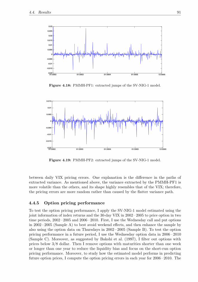
4.4. Results 91
01/2002 01/2003 01/2004 01/2005 12/2005-0.02
-0.015
-0.01
-0.005
0
0.005
0.01
0.015
0.02
0.025
0.03
Figure 4.18: PMMH-PF1: extracted jumps of the SV-NIG-1 model.
01/2002 01/2003 01/2004 01/2005 12/2005-0.02
-0.015
-0.01
-0.005
0
0.005
0.01
0.015
Figure 4.19: PMMH-PF2: extracted jumps of the SV-NIG-1 model.
between daily VIX pricing errors. One explanation is the di�erence in the paths ofextracted variance. As mentioned above, the variance extracted by the PMMH-PF1 ismore volatile than the others, and its shape highly resembles that of the VIX; therefore,the pricing errors are more random rather than caused by the flatter variance path.
4.4.5 Option pricing performanceTo test the option pricing performance, I apply the SV-NIG-1 model estimated using thejoint information of index returns and the 30-day VIX in 2002–2005 to price option in twotime periods, 2002–2005 and 2006–2010. First, I use the Wednesday call and put optionsin 2002–2005 (Sample A) to best avoid weekend e�ects, and then enhance the sample byalso using the option data on Thursdays in 2002–2005 (Sample B). To test the optionpricing performance in a future period, I use the Wednesday option data in 2006–2010(Sample C). Moreover, as suggested by Bakshi et al. (1997), I filter out options withprices below 3/8 dollar. Then I remove options with maturities shorter than one weekor longer than one year to reduce the liquidity bias and focus on the short-run optionpricing performance. Moreover, to study how the estimated model performs in predictingfuture option prices, I compute the option pricing errors in each year for 2006–2010. The
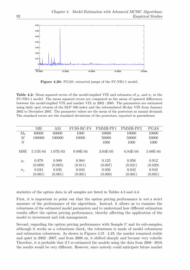
92Chapter 4. Model Estimation with Advanced MCMC Algorithms:
Empirical Studies
01/2002 01/2003 01/2004 01/2005 12/2005-0.01
0
0.01
0.02
0.03
0.04
0.05
0.06
0.07
Figure 4.20: PGAS: extracted jumps of the SV-NIG-1 model.
Table 4.2: Mean squared errors of the model-implied VIX and estimates of flÁ and ‡Á in theSV-NIG-1 model. The mean squared errors are computed as the mean of squared di�erencesbetween the model-implied VIX and market VIX in 2002–2005. The parameters are estimatedusing daily spot returns of the S&P 500 index and the reformulated 30-day VIX from January2002 to December 2005. The parameter values are the mean of the posteriors as annual decimals.The standard errors are the standard deviations of the posteriors, reported in parentheses.
MH AM FUSS-RC-P4 PMMH-PF1 PMMH-PF2 PGASM
0
60000 60000 1000 10000 10000 10000M 100000 100000 10000 50000 50000 50000N 1000 1000 1000
MSE 5.51E-04 1.07E-03 9.89E-04 3.04E-05 6.84E-04 5.08E-04
fl
Á
0.979 0.989 0.984 0.125 0.956 0.912(0.009) (0.005) (0.011) (0.007) (0.021) (0.020)
‡
Á
0.034 0.035 0.034 0.026 0.042 0.042(0.001) (0.001) (0.001) (0.000) (0.001) (0.001)
statistics of the option data in all samples are listed in Tables 4.3 and 4.4.
First, it is important to point out that the option pricing performance is not a strictmeasure of the performance of the algorithms. Instead, it allows us to examine therobustness of the estimated model parameters and to understand how di�erent estimationresults a�ect the option pricing performance, thereby a�ecting the application of themodel to investment and risk management.
Second, regarding the option pricing performance with Sample C and its sub-samples,although it works as a robustness check, the robustness is made of model robustnessand estimation robustness. As shown in Figures 4.21–4.23, the market remained stableand quiet in 2002–2007, and from 2008 on, it shifted sharply and became very volatile.Therefore, it is probable that if I re-estimated the models using the data from 2008–2010,the results would be very di�erent. However, since nobody could anticipate future market

4.4. Results 93
Table 4.3: Properties of options in Samples A, B, and C. Sample A: Wednesday call and putoptions in 2002–2005. Sample B: Thursday call and put options in 2002–2005. Sample C:Wednesday call and put options in 2006–2010. Options with prices below 3/8 dollar or maturitiesshorter than one week or longer than one year are filtered out. This table shows the number ofcontracts, the average price (in parentheses), and the average bid-ask spread {in braces}.
Sample A Sample B Sample CWed, 2002-2005 Thu, 2002-2005 Wed, 2006-2010
17660 17082 40543(21.56) (21.28) (26.45){1.25} {1.25} {1.74}
Table 4.4: Properties of options in Sub-Samples of Sample C. Options with prices below 3/8dollar or maturities shorter than one week or longer than one year are filtered out. This tableshows the number of contracts, the average price (in parentheses), and the average bid-ask spread{in braces}.
Sub-samples of Sample CWed, 2006 Wed, 2007 Wed, 2008 Wed, 2009 Wed, 2010
5872 7198 8889 8808 9776(18.70) (26.16) (35.81) (26.49) (22.77){1.12} {1.64} {2.38} {1.57} {1.76}
Table 4.5: Option VRMSEs for the SV-NIG-1 model. Sample A: Wednesday options fromJanuary 2002 to December 2005. Sample B: Thursday options from January 2002 to December2005. Sample C: Wednesday options from January 2006 to December 2010. Options with pricesbelow 3/8 dollar or maturities shorter than one week or longer than one year are filtered out.The option prices are computed by the Monte Carlo method with the technique of antitheticvariates. The number of Monte Carlo paths is 50, 000, and the model is discretised at dailyfrequency. In each sample, the number in bold is the lowest VRMSE.
Sample A Sample B Sample C
MH 3.019 3.150 4.042AM 3.067 3.212 4.185
FUSS-RC-P4 2.971 3.250 4.157PMMH-PF1 2.854 3.090 3.966PMMH-PF2 3.076 3.502 4.575
PGAS 3.207 3.627 4.849

94Chapter 4. Model Estimation with Advanced MCMC Algorithms:
Empirical StudiesTable 4.6: Option VRMSEs for the SV-NIG-1 model. The option samples are Wednesdayoptions from 2006 to 2010. Options with prices below 3/8 dollar or maturities shorter than oneweek or longer than one year are filtered out. The option prices are computed by the MonteCarlo method with the technique of antithetic variates. The number of Monte Carlo paths is50, 000, and the model is discretised at daily frequency. In each sample, the number in bold isthe lowest VRMSE.
2006 2007 2008 2009 2010MH 2.332 3.260 4.776 4.592 4.114AM 2.221 3.271 4.920 4.844 4.318
FUSS-RC-P4 2.292 3.382 4.819 4.748 4.322PMMH-PF1 2.244 3.224 4.708 4.513 4.005PMMH-PF2 2.571 3.848 5.134 5.177 4.883
PGAS 2.662 4.031 5.452 5.502 5.197
01/2002 2003 2004 2005 2006 2007 2008 2009 2010 12/20106.5
6.6
6.7
6.8
6.9
7
7.1
7.2
7.3
7.4
Figure 4.21: Daily returns of the S&P 500 index in 2002–2010.
changes, a model capable of explaining di�erent market conditions and an estimationmethod capable of identifying a robust parameter set will win the day.
The option pricing performance in Samples A, B, and C correlates highly with the fit tothe VIX. This is not surprising because the VIX index is constructed by option prices, andas mentioned above, the VIX is very informative of the risk-neutral dynamics of a model.Clearly, the PMMH-PF1, which performs best in the fit to the VIX, outperforms the othersin all three Samples A, B, and C. In pricing the options in the sub-samples of SampleC, all the algorithms perform better in 2006–2007 than in 2008–2010, because marketconditions in 2006–2007 were similar to those in 2002–2005, whereas in 2008–2010, themarket shifted dramatically.
Surprisingly, despite its good fit to the VIX, the PGAS performs worst in all threesamples A, B, and C. The reason is the unrealistic extracted jumps and jump-relatedparameters inconsistent with the data. In fact, the VIX index can be represented as adeterministic function of the spot variance and risk-neutral parameters; therefore, theimportance of appropriate jump-related parameters is relatively small in computing theVIX index, as the other risk-neutral parameters may compensate for the mis-speciationof the jumps-related parameters. However, when pricing options, I need to simulate
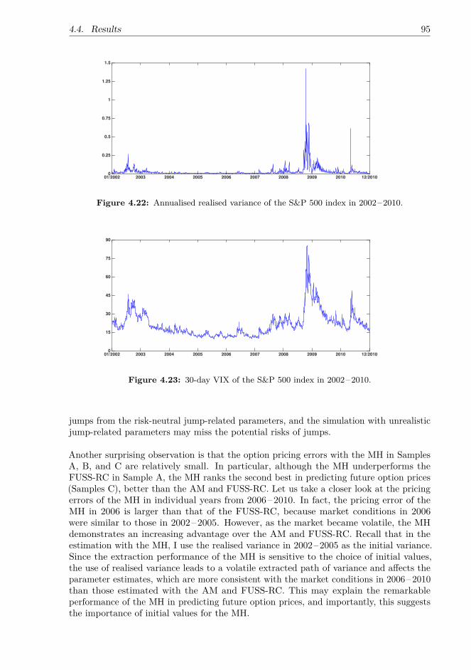
4.4. Results 95
01/2002 2003 2004 2005 2006 2007 2008 2009 2010 12/20100
0.25
0.5
0.75
1
1.25
1.5
Figure 4.22: Annualised realised variance of the S&P 500 index in 2002–2010.
01/2002 2003 2004 2005 2006 2007 2008 2009 2010 12/20100
15
30
45
60
75
90
Figure 4.23: 30-day VIX of the S&P 500 index in 2002–2010.
jumps from the risk-neutral jump-related parameters, and the simulation with unrealisticjump-related parameters may miss the potential risks of jumps.
Another surprising observation is that the option pricing errors with the MH in SamplesA, B, and C are relatively small. In particular, although the MH underperforms theFUSS-RC in Sample A, the MH ranks the second best in predicting future option prices(Samples C), better than the AM and FUSS-RC. Let us take a closer look at the pricingerrors of the MH in individual years from 2006–2010. In fact, the pricing error of theMH in 2006 is larger than that of the FUSS-RC, because market conditions in 2006were similar to those in 2002–2005. However, as the market became volatile, the MHdemonstrates an increasing advantage over the AM and FUSS-RC. Recall that in theestimation with the MH, I use the realised variance in 2002–2005 as the initial variance.Since the extraction performance of the MH is sensitive to the choice of initial values,the use of realised variance leads to a volatile extracted path of variance and a�ects theparameter estimates, which are more consistent with the market conditions in 2006–2010than those estimated with the AM and FUSS-RC. This may explain the remarkableperformance of the MH in predicting future option prices, and importantly, this suggeststhe importance of initial values for the MH.

96Chapter 4. Model Estimation with Advanced MCMC Algorithms:
Empirical Studies
4.5 Discussion
In this chapter, I apply the advanced MCMC algorithms to estimate the SV-NIG-1 modelusing the joint information of the S&P 500 index returns and daily 30-day VIX data fromJanuary 2002 to December 2005. The algorithms comprise the AM, the FUSS-RC withpruning type 4, the PMMH-PF1/PF2, and PGAS, and their performance is compared tothat of the conventional random-walk MH algorithm.
When extracting the strongly autocorrelated spot variance, the adaptive proposal usedin the AM increases the acceptance rate of the MH and reduce the autocorrelationbetween samples of the spot variance. The FUSS-RC and PGAS further improve theextraction of the spot variance in that the ACFs of the spot variance extracted by theFUSS-RC and PGAS drop sharply, which is in line with the results of Martino et al.(2015) and Lindsten et al. (2014). Furthermore, the FUSS-RC even reduces the ACFwith negative autocorrelation, suggesting that this algorithm is e�cient in generatinggood representatives of the target distribution. In contrast, the acceptance rates ofthe PMMH-PF1 and the PMMH-PF2 are very low owing to the model specification ofindependent NIG return jumps.
Moreover, the choice of estimation methods may a�ect the option pricing performance. Inparticular, the model-implied VIX with the PMMH-PF1 almost completely coincides withthe market VIX; therefore, since the option pricing performance correlates highly with thefit to the VIX, the PMMH-PF1 outperforms the other algorithms in the option pricingperformance in all three samples. In contrast, the PGAS performs worst in all threesamples owing to the poorly identified jump-related parameters under the risk-neutralmeasure. The MH ranks the second best in predicting option prices due to the use ofrealised variance as the initial variance, which makes the estimation results more consistentwith the market conditions in 2006–2010 than those estimated with other algorithms.
To sum up, the PGAS can cope with strong dependence between parameters and statevariables, and if one emphasises the fit to observations that can be represented as afunction of model parameters and state variables, the PMMH-PF1 is very competitive.However, the performance of the PMMH-PF1 and the PGAS may be weakened by theinclusion of independent jumps. In contrast, the other algorithms are less vulnerable tothe inclusion of independent jumps, and they achieve a stable performance in parameterestimation, extraction of state variables, fit to the VIX, and option pricing. In particular,an appropriate choice of initial values for state variables may significantly improve theperformance of the MH; moreover, the FUSS-RC is very competitive because it can improvethe estimation performance of the MH and AM and generate good representatives ofthe target distribution of state variables in the presence of high dimensions and a strongdependence structure.
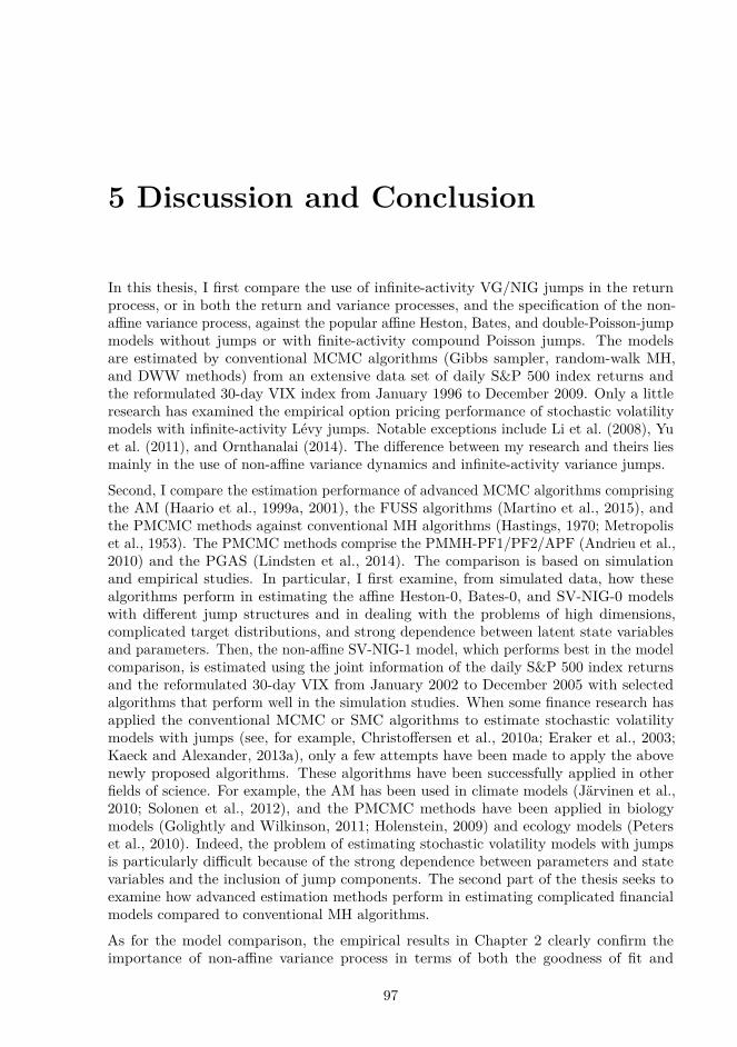
5 Discussion and Conclusion
In this thesis, I first compare the use of infinite-activity VG/NIG jumps in the returnprocess, or in both the return and variance processes, and the specification of the non-a�ne variance process, against the popular a�ne Heston, Bates, and double-Poisson-jumpmodels without jumps or with finite-activity compound Poisson jumps. The modelsare estimated by conventional MCMC algorithms (Gibbs sampler, random-walk MH,and DWW methods) from an extensive data set of daily S&P 500 index returns andthe reformulated 30-day VIX index from January 1996 to December 2009. Only a littleresearch has examined the empirical option pricing performance of stochastic volatilitymodels with infinite-activity Lévy jumps. Notable exceptions include Li et al. (2008), Yuet al. (2011), and Ornthanalai (2014). The di�erence between my research and theirs liesmainly in the use of non-a�ne variance dynamics and infinite-activity variance jumps.
Second, I compare the estimation performance of advanced MCMC algorithms comprisingthe AM (Haario et al., 1999a, 2001), the FUSS algorithms (Martino et al., 2015), andthe PMCMC methods against conventional MH algorithms (Hastings, 1970; Metropoliset al., 1953). The PMCMC methods comprise the PMMH-PF1/PF2/APF (Andrieu et al.,2010) and the PGAS (Lindsten et al., 2014). The comparison is based on simulationand empirical studies. In particular, I first examine, from simulated data, how thesealgorithms perform in estimating the a�ne Heston-0, Bates-0, and SV-NIG-0 modelswith di�erent jump structures and in dealing with the problems of high dimensions,complicated target distributions, and strong dependence between latent state variablesand parameters. Then, the non-a�ne SV-NIG-1 model, which performs best in the modelcomparison, is estimated using the joint information of the daily S&P 500 index returnsand the reformulated 30-day VIX from January 2002 to December 2005 with selectedalgorithms that perform well in the simulation studies. When some finance research hasapplied the conventional MCMC or SMC algorithms to estimate stochastic volatilitymodels with jumps (see, for example, Christo�ersen et al., 2010a; Eraker et al., 2003;Kaeck and Alexander, 2013a), only a few attempts have been made to apply the abovenewly proposed algorithms. These algorithms have been successfully applied in otherfields of science. For example, the AM has been used in climate models (Järvinen et al.,2010; Solonen et al., 2012), and the PMCMC methods have been applied in biologymodels (Golightly and Wilkinson, 2011; Holenstein, 2009) and ecology models (Peterset al., 2010). Indeed, the problem of estimating stochastic volatility models with jumpsis particularly di�cult because of the strong dependence between parameters and statevariables and the inclusion of jump components. The second part of the thesis seeks toexamine how advanced estimation methods perform in estimating complicated financialmodels compared to conventional MH algorithms.
As for the model comparison, the empirical results in Chapter 2 clearly confirm theimportance of non-a�ne variance process in terms of both the goodness of fit and
97

98 Chapter 5. Discussion and Conclusion
option pricing, as noted in the literature (see, for example, Christo�ersen et al., 2010a;Kaeck and Alexander, 2012). Moreover, the non-a�ne variance specification can improvemodel robustness, whereas a�ne variance dynamics may lead to unstable option pricingperformance across di�erent option samples. More importantly, the improvement broughtby the infinite-activity Lévy jumps, which has not been widely recognised, is criticalwith the non-a�ne variance specification. The empirical results indicate that the infinite-activity VG/NIG return jumps generate more realistic index dynamics and option prices,and capture the uncertainty of future jumps better, which is missed by the finite-activitycompound Poisson jumps. Furthermore, the role of infinite-activity variance jumps is lessimportant than that of infinite-activity return jumps. The empirical results show thatthe SV-NIG-1 markedly outperforms the others in pricing options and the SV-VG-NIG-1achieves the best performance in goodness of fit. However, overall, the SV-VG-NIG-1 andSV-NIG-1 models are comparable, and considering the extra model complexity of theSV-VG-NIG-1, I conclude that the parsimonious model SV-NIG-1 is the more competitiveone.
As for the algorithm comparison, the results of the simulation studies in Chapter 3suggest that di�erent jump structures may significantly a�ect the estimation performanceof the algorithms. When estimating the Bates-0 model, all the algorithms are able toextract the compound Poisson jumps; however, the inclusion of rare large jumps reducesthe acceptance rate of the PMCMC methods and worsens their estimation performance.Moreover, the extraction of the infinite-activity NIG jumps is di�cult for all the algorithms,and the inclusion of NIG jumps makes the estimation of parameters and the extractionof variance very challenging. Considering the complexity and computational costs ofdi�erent algorithms, I conclude that for models with simple specifications, the MHis very competitive because of its low computational cost. The AM further improvesthe performance of the MH because it can significantly raise the acceptance rate andaccelerate the convergence of the chain by an online-tuned adaptive proposal. However,the MH and AM are less capable of dealing with complicated model specifications. TheFUSS algorithms are particularly competitive in coping with strong dependence betweenstate variables and in generating virtually independent samples from complicated targetdistributions, as noted in Martino et al. (2015). Generally, they achieve a good mixingwith the smallest MCMC runs, and their performance is stable and excellent regardless ofmodel specifications; however, they are relatively computationally expensive. In contrast,the PMCMC methods are computationally cheap and very e�cient in mixing, and inthe simulation studies, they outperform the FUSS algorithms in estimating the Heston-0and SV-NIG-0 models. However, the PMCMC methods are more vulnerable to modelspecifications than the other algorithms; in particular, the inclusion of large independentjumps may significantly reduce the e�ciency of the PMCMC methods.
The results of the empirical studies in Chapter 4 show that in extracting the strongly au-tocorrelated spot variance, the adaptive proposal used in the AM increases the acceptancerate of the MH and reduces the autocorrelation between samples of the spot variance.The FUSS-RC and PGAS further improve the extraction of the spot variance in that theACFs of the spot variance extracted by the FUSS-RC and PGAS drop sharply, which isin line with the results in Martino et al. (2015) and Lindsten et al. (2014). Furthermore,the FUSS-RC even reduces the ACF with negative autocorrelation, suggesting that thisalgorithm is e�cient in generating good representatives of the target distribution. Incontrast, the acceptance rates of the PMMH algorithms are very low owing to the modelspecification of independent NIG jumps in the return process, and the jump-relatedparameters are poorly identified by the PGAS. This suggests that, compared to the MH,
99
AM, and FUSS-RC, the PMCMC methods are less capable of extracting independentjumps; moreover, the inclusion of independent jumps may negatively a�ect their esti-mation performance. Furthermore, the choice of estimation methods a�ects the optionpricing performance. In particular, the model-implied VIX with the PMMH-PF1 almostcompletely coincides with the market VIX; therefore, since the option pricing performancecorrelated highly with the fit to the VIX, the PMMH-PF1 outperforms the others in theoption pricing performance in all three option samples. In contract, the PGAS performsworst in all three samples owing to the poorly identified jump-related parameters underthe risk-neutral measure. The MH ranks the second best in predicting option prices dueto the use of the realised variance as the initial variance in the estimation, which leads toan estimation result consistent with the market conditions in 2006–2010.
In conclusion, according to the empirical results in the model comparison, there is clearevidence for the importance of the infinite-activity return jumps and non-a�ne variancedynamics in terms of the goodness of fit and option pricing performance, and the role ofvariance jumps is less important than that of return jumps. In particular, a relativelyparsimonious model with infinite-activity NIG return jumps and non-a�ne variancedynamics is very competitive. The results of the simulation and empirical studies on thealgorithm comparison suggest that each estimation algorithm has its own strengths anddrawbacks, and no single algorithm has shown an overwhelming advantage. The PMCMCmethods perform well in the presence of high dimensions and strong dependence betweenparameters and latent state variables, and if one emphasises the fit to data that can berepresented as a function of model parameters and state variables, the PMMH-PF1 isparticularly competitive; however, their performance may be weakened by the inclusionof large independent jumps. Despite the high computational cost, the FUSS algorithmsare particularly competitive in generating virtually independent samples and in achievingthe fastest mixing with a fixed number of MCMC runs, and their performance is stableregardless of model specifications.
Finally, in future research, it would be interesting to use a volatility term structure toidentify the variance dynamics and to use a second factor to model the long-term mean ofvariance, as in Kaeck and Alexander (2012). Moreover, as pointed out in Andersen et al.(2014), a left tail factor is critical in forecasting the variance risk premium dynamics,and the time-varying jump risk premia improve the risk-neutral dynamics. It would beinteresting to add the specification of time-varying jump risk premia to the current models,for example, by making the jump-related parameters time-varying, or by assuming anotherfactor. As for the estimation methods, a number of extensions to the PMCMC methods,as mentioned in Andrieu et al. (2010), may further improve the estimation performance.In particular, a lot of literature has contributed to improving SMC algorithms, and thetechniques discussed in the SMC literature, such as the PF scheme dealing with anomalousobservations (Maiz et al., 2012), may be applied to the SMC update in the PMCMCmethods. Moreover, the FUSS algorithms prove e�ective in this thesis; however, their highcomputational cost may limit their application. Therefore, it would be helpful to makethe FUSS algorithms more e�cient in pruning support points and constructing proposals.Further, the particle learning (Carvalho et al., 2010) has shown to be competitive to theMCMC, and this would be a promising direction for future research.


Bibliography
Ait-Sahalia, Y. and Kimmel, R., “Maximum likelihood estimation of stochastic volatilitymodels,” Journal of Financial Economics, vol. 83, no. 2, pp. 413–452, 2007.
Amengual, D., “The term structure of variance risk premia,” Princeton University, 2009.
An, S. and Schorfheide, F., “Bayesian analysis of DSGE models,” Econometric reviews,vol. 26, no. 2-4, pp. 113–172, 2007.
Andersen, T. G., Fusari, N., and Todorov, V., “The risk premia embedded in indexoptions,” Working paper, Northwestern University, 2014.
Andersen, T. G. and Sørensen, B. E., “GMM estimation of a stochastic volatility model:a Monte Carlo study,” Journal of Business & Economic Statistics, vol. 14, no. 3, pp.328–352, 1996.
Andrieu, C., Doucet, A., and Holenstein, R., “Particle Markov Chain Monte Carlomethods,” Journal of the Royal Statistical Society: Series B (Statistical Methodology),vol. 72, no. 3, pp. 269–342, 2010.
Bakshi, G., Cao, C., and Chen, Z., “Empirical performance of alternative option pricingmodels,” The Journal of Finance, vol. 52, no. 5, pp. 2003–2049, 1997.
Barndor�-Nielsen, O. E., “Normal inverse Gaussian distributions and stochastic volatilitymodelling,” Scandinavian Journal of statistics, vol. 24, no. 1, pp. 1–13, 1997.
– – – , “Processes of normal inverse Gaussian type,” Finance and stochastics, vol. 2, no. 1,pp. 41–68, 1997.
Bates, D. S., “Jumps and stochastic volatility: Exchange rate processes implicit indeutsche mark options,” Review of financial studies, vol. 9, no. 1, pp. 69–107, 1996.
– – – , “Post-’87 crash fears in the S&P 500 futures option market,” Journal of Econo-metrics, vol. 94, no. 1, pp. 181–238, 2000.
– – – , “Maximum likelihood estimation of latent a�ne processes,” Review of FinancialStudies, vol. 19, no. 3, pp. 909–965, 2006.
– – – , “US stock market crash risk, 1926–2010,” Journal of Financial Economics, vol.105, no. 2, pp. 229–259, 2012.
Berg, A., Meyer, R., and Yu, J., “Deviance information criterion for comparing stochasticvolatility models,” Journal of Business & Economic Statistics, vol. 22, no. 1, pp.107–120, 2004.
101

102 Bibliography
Berzuini, C., Best, N. G., Gilks, W. R., and Larizza, C., “Dynamic conditional inde-pendence models and Markov Chain Monte Carlo methods,” Journal of the AmericanStatistical Association, vol. 92, no. 440, pp. 1403–1412, 1997.
Black, F. and Scholes, M., “The pricing of options and corporate liabilities,” The journalof political economy, pp. 637–654, 1973.
Broadie, M., Chernov, M., and Johannes, M., “Model specification and risk premia:Evidence from futures options,” The Journal of Finance, vol. 62, no. 3, pp. 1453–1490,2007.
Carr, P. and Madan, D. B., “Option valuation using the fast fourier transform,” Journalof computational finance, vol. 2, no. 4, pp. 61–73, 1999.
– – – , “Optimal positioning in derivative securities,” Quantitative Finance, vol. 1, pp.19–37, 2001.
Carr, P. and Wu, L., “The finite moment log stable process and option pricing,” Journalof Finance, vol. 58, pp. 753–777, 2003.
– – – , “Time-changed Lévy processes and option pricing,” Journal of Financial Economics,vol. 71, no. 1, pp. 113–141, 2004.
Carr, P., Geman, H., and Madan, D. B., “The fine structure of asset returns: An empiricalinvestigation,” Journal of Business, vol. 75, pp. 305–332, 2002.
Carr, P., Geman, H., Madan, D. B., and Yor, M., “Stochastic volatility for Lévy processes,”Mathematical Finance, vol. 13, no. 3, pp. 345–382, 2003.
Carvalho, C., Johannes, M., Lopes, H. F., and Polson, N., “Particle learning and smooth-ing,” Statistical Science, vol. 25, no. 1, pp. 88–106, 2010.
Chacko, G. and Viceira, L. M., “Spectral GMM estimation of continuous-time processes,”Journal of Econometrics, vol. 116, no. 1, pp. 259–292, 2003.
Chernov, M. and Ghysels, E., “A study towards a unified approach to the joint estimationof objective and risk neutral measures for the purpose of options valuation,” Journal offinancial economics, vol. 56, no. 3, pp. 407–458, 2000.
Chopin, N. and Singh, S. S., “On the particle Gibbs sampler,” arXiv preprintarXiv:1304.1887, 2013.
Christo�ersen, P. and Jacobs, K., “Which GARCH model for option valuation?” Man-agement Science, vol. 50, no. 9, pp. 1204–1221, 2004.
Christo�ersen, P., Dorion, C., Jacobs, K., and Wang, Y., “Volatility components, a�nerestrictions, and non-normal innovations,” Journal of Business & Economic Statistics,vol. 28, no. 4, pp. 483–502, 2010.
Christo�ersen, P., Jacobs, K., and Mimouni, K., “Volatility dynamics for the S&P500:evidence from realized volatility, daily returns, and option prices,” Review of FinancialStudies, p. hhq032, 2010.
Christo�ersen, P., Jacobs, K., and Ornthanalai, C., “GARCH option valuation: Theoryand evidence,” Available at SSRN 2054859, 2013.

Bibliography 103
Creal, D., “Analysis of filtering and smoothing algorithms for Lévy-driven stochasticvolatility models,” Computational Statistics & Data Analysis, vol. 52, no. 6, pp. 2863–2876, 2008.
– – – , “A survey of sequential Monte Carlo methods for economics and finance,” Econo-metric Reviews, vol. 31, no. 3, pp. 245–296, 2012.
Damlen, P., Wakefield, J., and Walker, S., “Gibbs sampling for Bayesian non-conjugateand hierarchical models by using auxiliary variables,” Journal of the Royal StatisticalSociety: Series B (Statistical Methodology), vol. 61, no. 2, pp. 331–344, 1999.
Djuric, P. M., Kotecha, J. H., Zhang, J., Huang, Y., Ghirmai, T., Bugallo, M. F., andMiguez, J., “Particle filtering,” Signal Processing Magazine, IEEE, vol. 20, no. 5, pp.19–38, 2003.
Doucet, A., De Freitas, N., and Gordon, N., An introduction to sequential Monte Carlomethods. Springer, 2001.
Duan, J. C. and Yeh, C. Y., “Jump and volatility risk premiums implied by VIX,” Journalof Economic Dynamics and Control, vol. 34, no. 11, pp. 2232–2244, 2010.
– – – , “Price and volatility dynamics implied by the VIX term structure,” Available atSSRN 1788252, 2011.
Du�e, D., Pan, J., and Singleton, K., “Transform analysis and asset pricing for a�nejump-di�usions,” Econometrica, vol. 68, no. 6, pp. 1343–1376, 2000.
Du�e, D., FilipoviÊ, D., and Schachermayer, W., “A�ne processes and applications infinance,” Annals of applied probability, pp. 984–1053, 2003.
Eberlein, E. and Madan, D. B., “On correlating Lévy processes,” Robert H. Smith SchoolResearch Paper No. RHS, pp. 06–118, 2009.
Eraker, B., “Do stock prices and volatility jump? Reconciling evidence from spot andoption prices,” The Journal of Finance, vol. 59, no. 3, pp. 1367–1404, 2004.
Eraker, B., Johannes, M., and Polson, N., “The impact of jumps in volatility and returns,”The Journal of Finance, vol. 58, no. 3, pp. 1269–1300, 2003.
Fernández-Villaverde, J. and Rubio-Ramírez, J. F., “Estimating dynamic equilibriumeconomies: linear versus nonlinear likelihood,” Journal of Applied Econometrics, vol. 20,no. 7, pp. 891–910, 2005.
Gelman, A., Roberts, G., and Gilks, W., “E�cient Metropolis jumping hules,” Bayesianstatistics, vol. 5, no. 599-608, p. 42, 1996.
Gilks, W. R., “Derivative-free Adaptive Rejection Sampling for Gibbs Sampling,” BayesianStatistics, vol. 4, pp. 641–649, 1992.
Gilks, W. R. and Wild, P., “Adaptive Rejection Sampling for Gibbs Sampling,” AppliedStatistics, vol. 41, no. 2, pp. 337–348, 1992.
Gilks, W. R., Best, N. G., and Tan, K. K. C., “Adaptive Rejection Metropolis Samplingwithin Gibbs Sampling,” Applied Statistics, vol. 44, no. 4, pp. 455–472, 1995.

104 Bibliography
Gilks, W. R., Neal, R., Best, N. G., and Tan, K. K. C., “Corrigidum: Adaptive RejectionMetropolis Sampling within Gibbs Sampling,” Applied Statistics, vol. 46, no. 4, pp.541–542, 1997.
Golightly, A. and Wilkinson, D. J., “Bayesian parameter inference for stochastic bio-chemical network models using particle markov chain monte carlo,” Interface focus, p.rsfs20110047, 2011.
Gordon, N. J., Salmond, D. J., and Smith, A. F., “Novel approach to nonlinear/non-Gaussian Bayesian state estimation,” in IEE Proceedings F (Radar and Signal Process-ing), vol. 140, no. 2. IET, 1993, pp. 107–113.
Haario, H., Saksman, E., and Tamminen, J., “Adaptive proposal distribution for randomwalk Metropolis algorithm,” Computational Statistics, vol. 14, pp. 375–395, 1999.
– – – , “Adaptive proposal distribution for random walk Metropolis algorithm,” Computa-tional Statistics, vol. 14, no. 3, pp. 375–396, 1999.
– – – , “An adaptive Metropolis algorithm,” Bernoulli, pp. 223–242, 2001.
Haario, H., Laine, M., Mira, A., and Saksman, E., “DRAM: e�cient adaptive MCMC,”Statistics and Computing, vol. 16, no. 4, pp. 339–354, 2006.
Hammersley, J. M. and Cli�ord, P., “Markov fields on finite graphs and lattices,” 1971.
Hastings, W. K., “Monte carlo sampling methods using markov chains and their applica-tions,” Biometrika, vol. 57, no. 1, pp. 97–109, 1970.
Heston, S. L., “A closed-form solution for options with stochastic volatility with appli-cations to bond and currency options,” Review of Financial Studies, vol. 6, no. 2, pp.327–343, 1993.
Heston, S. L. and Nandi, S., “A closed-form GARCH option valuation model,” Review ofFinancial Studies, vol. 13, no. 3, pp. 585–625, 2000.
Holenstein, R., “Particle markov chain monte carlo,” Ph.D. dissertation, The UniversityOf British Columbia (Vancouver, 2009.
Ignatieva, K., Rodrigues, P., and Seeger, N., “Stochastic volatility and jumps: Expo-nentially a�ne yes or no? An empirical analysis of S&P500 dynamics,” Journal ofBusiness and Economic Statistics, 2015, forthcoming.
Jacquier, E., Polson, N. G., and Rossi, P. E., “Bayesian analysis of stochastic volatilitymodels,” Journal of Business & Economic Statistics, vol. 20, no. 1, pp. 69–87, 2002.
Jacquier, E., Johannes, M., and Polson, N., “MCMC maximum likelihood for latent statemodels,” Journal of Econometrics, vol. 137, no. 2, pp. 615–640, 2007.
Järvinen, H., Räisänen, P., Laine, M., Tamminen, J., Ilin, A., Oja, E., Solonen, A., andHaario, H., “Estimation of echam5 climate model closure parameters with adaptivemcmc,” Atmospheric Chemistry and Physics, vol. 10, no. 20, pp. 9993–10 002, 2010.
Johannes, M. and Polson, N., “MCMC methods for continuous-time financial economet-rics,” Available at SSRN 480461, 2003.

Bibliography 105
Johansen, A. M., Doucet, A., and Davy, M., “Particle methods for maximum likelihoodestimation in latent variable models,” Statistics and Computing, vol. 18, no. 1, pp.47–57, 2008.
Jones, C. S., “The dynamics of stochastic volatility: evidence from underlying and optionsmarkets,” Journal of Econometrics, vol. 116, no. 1, pp. 181–224, 2003.
Kaeck, A. and Alexander, C., “Volatility dynamics for the S&P500: Further evidencefrom non-a�ne, multi-factor jump di�usions,” Journal of Banking & Finance, vol. 36,no. 11, pp. 3110–3121, 2012.
– – – , “Stochastic volatility jump-di�usions for European equity index dynamics,” Euro-pean Financial Management, vol. 19, no. 3, pp. 470–496, 2013.
– – – , “Continuous-time VIX dynamics: On the role of stochastic volatility of volatility,”International Review of Financial Analysis, vol. 28, pp. 46–56, 2013.
Kallsen, J., “A didactic note on a�ne stochastic volatility models,” in From stochasticcalculus to mathematical finance. Springer, 2006, pp. 343–368.
Kanniainen, J., Lin, B., and Yang, H., “Estimating and using GARCH models with VIXdata for option valuation,” Journal of Banking & Finance, vol. 43, pp. 200–211, 2014.
Koch, K. R., “Gibbs sampler by sampling-importance-resampling,” Journal of Geodesy,vol. 81, no. 9, pp. 581–591, 2007.
Lewis, A. L., “Option valuation under stochastic volatility,” Option Valuation underStochastic Volatility, 2000.
Li, H., Wells, M., and Yu, C., “A Bayesian analysis of return dynamics with Lévy jumps,”Review of Financial Studies, vol. 21, no. 5, pp. 2345–2378, 2008.
Li, J., “Sequential Bayesian analysis of time-changed infinite activity derivatives pricingmodels,” Journal of Business & Economic Statistics, vol. 29, no. 4, 2011.
Liang, F., Liu, C., and Caroll, R., Advanced Markov Chain Monte Carlo Methods:Learning from Past Samples. England: Wiley Series in Computational Statistics, 2010.
Lindsten, F. and Schön, T. B., “Backward simulation methods for Monte Carlo statisticalinference.” Foundations and Trends in Machine Learning, vol. 6, no. 1, pp. 1–143, 2013.
Lindsten, F., Jordan, M. I., and Schön, T. B., “Particle Gibbs with ancestor sampling,”The Journal of Machine Learning Research, vol. 15, no. 1, pp. 2145–2184, 2014.
Liu, J. S., Monte Carlo Strategies in Scientific Computing. Springer, 2004.
Liu, J. S. and Chen, R., “Sequential monte carlo methods for dynamic systems,” Journalof the American statistical association, vol. 93, no. 443, pp. 1032–1044, 1998.
Madan, D., Carr, P., and Chang, E., “The Variance Gamma process and option pricing,”European finance review, vol. 2, no. 1, pp. 79–105, 1998.
Maiz, C. S., Molanes-Lopez, E. M., Míguez, J., and DjuriÊ, P. M., “A particle filteringscheme for processing time series corrupted by outliers,” Signal Processing, IEEETransactions on, vol. 60, no. 9, pp. 4611–4627, 2012.

106 Bibliography
Martino, L., Read, J., and Luengo, D., “Improved adaptive rejection Metropolis samplingalgorithms,” arXiv:1205.5494, pp. 1–32, Oct. 2012.
Martino, L., Casarin, R., Leisen, F., and Luengo, D., “Adaptive sticky generalizedMetropolis,” arXiv:1308.3779, pp. 1–44, Sep. 2013.
Martino, L., Read, J., and luengo, D., “Independent doubly adaptive rejection Metropolissampling,” in Proc. of IEEE International Conference on Acoustics, Speech, and SignalProcessing (ICASSP), 2014, pp. 8048–8052.
Martino, L., Yang, H., Luengo, D., Kanniainen, J., and Corander, J., “A fast universalself-tuned sampler within Gibbs sampling,” Digital Signal Processing, 2015, forthcoming.
Metropolis, N., Rosenbluth, A., Rosenbluth, M., Teller, A., and Teller, E., “Equations ofstate calculations by fast computing machines,” Journal of Chemical Physics, vol. 21,pp. 1087–1091, 1953.
Meyer, R., Cai, B., and Perron, F., “Adaptive rejection Metropolis sampling usingLagrange interpolation polynomials of degree 2,” Computational Statistics and DataAnalysis, vol. 52, no. 7, pp. 3408–3423, March 2008.
Müller, P., “Monte Carlo integration in general dynamic models,” Contemporary Mathe-matics, vol. 115, pp. 145–163, 1991.
Ornthanalai, C., “Lévy jump risk: Evidence from options and returns,” Journal ofFinancial Economics, vol. 112, no. 1, pp. 69–90, 2014.
Pan, J., “The jump-risk premia implicit in options: Evidence from an integrated time-seriesstudy,” Journal of Financial Economics, vol. 63, no. 1, pp. 3–50, 2002.
Peters, G. W., Hosack, G. R., and Hayes, K. R., “Ecological non-linear state spacemodel selection via adaptive particle Markov Chain Monte Carlo (AdPMCMC),” arXivpreprint arXiv:1005.2238, 2010.
Pitt, M. K. and Shephard, N., “Auxiliary variable based particle filters,” in SequentialMonte Carlo methods in practice. Springer, 2001, pp. 273–293.
Robert, C. P. and Casella, G., Monte Carlo Statistical Methods. Springer, 2004.
Sato, K., “Lévy processes and infinite divisibility,” 1999.
Solonen, A., Ollinaho, P., Laine, M., Haario, H., Tamminen, J., Järvinen, H. et al.,“E�cient mcmc for climate model parameter estimation: Parallel adaptive chains andearly rejection,” Bayesian Analysis, vol. 7, no. 3, pp. 715–736, 2012.
Spiegelhalter, D. J., Best, N. G., Carlin, B. P., and Van Der Linde, A., “Bayesianmeasures of model complexity and fit,” Journal of the Royal Statistical Society: SeriesB (Statistical Methodology), vol. 64, no. 4, pp. 583–639, 2002.
Storvik, G., “Particle filters for state-space models with the presence of unknown staticparameters,” Signal Processing, IEEE Transactions on, vol. 50, no. 2, pp. 281–289,2002.
Tankov, P., Financial modelling with jump processes. CRC press, 2003.

Bibliography 107
Wu, X., Stochastic volatility with Lévy processes: calibration and pricing. University ofMaryland, 2005.
Yu, L., Li, H., and Wells, M. T., “MCMC estimation of Lévy jump models using stockand option prices,” Mathematical Finance, vol. 21, no. 3, pp. 383–422, 2011.


Appendices


A Simulation Studies: ExtractedVariance
In this appendix, I report the spot variance extracted by di�erent algorithms in theHeston-0, Bates-0, and SV-NIG-0 models. The extracted path is plotted in a blue solidline and the true path is plotted in a red dotted-dashed line.
111

112 A Simulation Studies: Extracted Variance
0 50 100 150 200 2500
0.005
0.01
0.015
0.02
0.025
0.03
0.035
simulated variancefiltered variance
Figure A.1: Random-walk MH: extracted variance of the Heston-0 model.
0 50 100 150 200 2500
0.005
0.01
0.015
0.02
0.025
0.03
0.035
simulated variancefiltered variance
Figure A.2: AM: extracted variance of the Heston-0 model.
0 50 100 150 200 2500
0.005
0.01
0.015
0.02
0.025
0.03
0.035
simulated variancefiltered variance
Figure A.3: FUSS-RC-P4: extracted variance of the Heston-0 model.
0 50 100 150 200 2500
0.005
0.01
0.015
0.02
0.025
0.03
0.035
simulated variancefiltered variance
Figure A.4: FUSS-MH-P4: extracted variance of the Heston-0 model.

113
0 50 100 150 200 2500
0.005
0.01
0.015
0.02
0.025
0.03
0.035
simulated variancefiltered variance
Figure A.5: PMMH-PF1: extracted variance of the Heston-0 model.
0 50 100 150 200 2500
0.005
0.01
0.015
0.02
0.025
0.03
0.035simulated path
filtered path
Figure A.6: PMMH-PF2: extracted variance of the Heston-0 model.
0 50 100 150 200 2500
0.005
0.01
0.015
0.02
0.025
0.03
0.035simulated path
filtered path
Figure A.7: PGAS: extracted variance of the Heston-0 model.
0 50 100 150 200 2500
0.01
0.02
0.03
0.04
0.05
0.06
simulated path
filtered path
Figure A.8: Random-walk MH: extracted variance of the Bates-0 model.
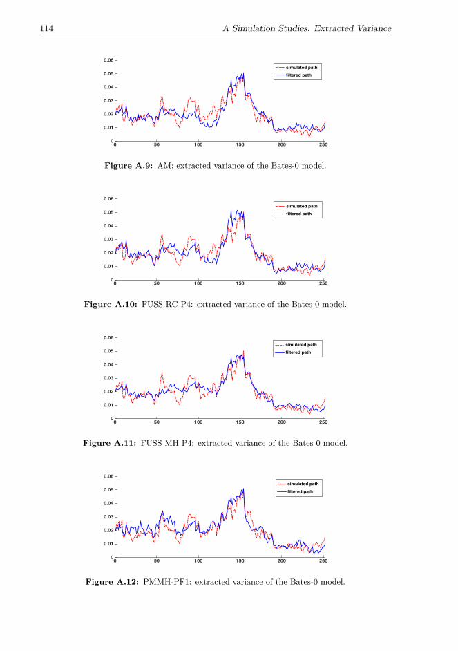
114 A Simulation Studies: Extracted Variance
0 50 100 150 200 2500
0.01
0.02
0.03
0.04
0.05
0.06
simulated path
filtered path
Figure A.9: AM: extracted variance of the Bates-0 model.
0 50 100 150 200 2500
0.01
0.02
0.03
0.04
0.05
0.06
simulated path
filtered path
Figure A.10: FUSS-RC-P4: extracted variance of the Bates-0 model.
0 50 100 150 200 2500
0.01
0.02
0.03
0.04
0.05
0.06
simulated path
filtered path
Figure A.11: FUSS-MH-P4: extracted variance of the Bates-0 model.
0 50 100 150 200 2500
0.01
0.02
0.03
0.04
0.05
0.06
simulated path
filtered path
Figure A.12: PMMH-PF1: extracted variance of the Bates-0 model.

115
0 50 100 150 200 2500.01
0.015
0.02
0.025
0.03
0.035
0.04
simulated path
filtered path
Figure A.13: Random-walk MH: extracted variance of the SV-NIG-0 model.
0 50 100 150 200 2500.01
0.015
0.02
0.025
0.03
0.035
0.04
simulated path
filtered path
Figure A.14: AM: extracted variance of the SV-NIG-0 model.
0 50 100 150 200 2500.01
0.015
0.02
0.025
0.03
0.035
0.04
simulated path
filtered path
Figure A.15: FUSS-MH-P4: extracted variance of the SV-NIG-0 model.
0 50 100 150 200 2500.01
0.015
0.02
0.025
0.03
0.035
0.04
simulated path
filtered path
Figure A.16: FUSS-RC-P4: extracted variance of the SV-NIG-0 model.

116 A Simulation Studies: Extracted Variance
0 50 100 150 200 2500.01
0.015
0.02
0.025
0.03
0.035
0.04
simulated path
filtered path
Figure A.17: PMMH-PF1: extracted variance of the SV-NIG-0 model.
0 50 100 150 200 2500.01
0.015
0.02
0.025
0.03
0.035
0.04
simulated path
filtered path
Figure A.18: PGAS: extracted variance of the SV-NIG-0 model.

B Simulation Studies: ExtractedJumps
In this appendix, I report the jumps extracted by di�erent algorithms in the Bates-0and SV-NIG-0 models. The extracted jumps are plotted in a blue solid line and the truejumps are plotted in a red dotted-dashed line.
117
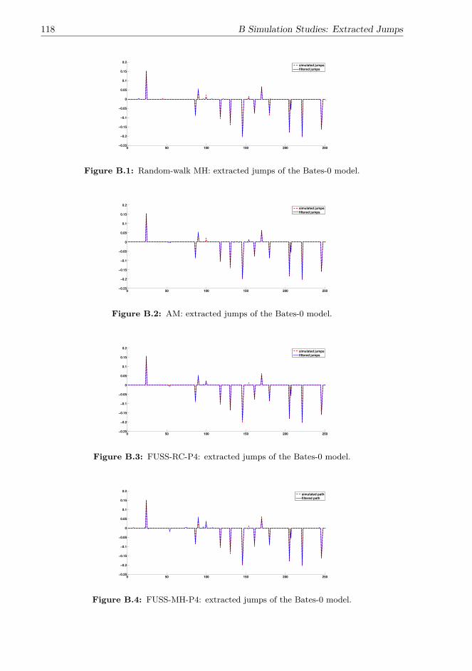
118 B Simulation Studies: Extracted Jumps
0 50 100 150 200 250−0.25
−0.2
−0.15
−0.1
−0.05
0
0.05
0.1
0.15
0.2
simulated jumpsfiltered jumps
Figure B.1: Random-walk MH: extracted jumps of the Bates-0 model.
0 50 100 150 200 250−0.25
−0.2
−0.15
−0.1
−0.05
0
0.05
0.1
0.15
0.2
simulated jumpsfiltered jumps
Figure B.2: AM: extracted jumps of the Bates-0 model.
0 50 100 150 200 250−0.25
−0.2
−0.15
−0.1
−0.05
0
0.05
0.1
0.15
0.2
simulated jumpsfiltered jumps
Figure B.3: FUSS-RC-P4: extracted jumps of the Bates-0 model.
0 50 100 150 200 250−0.25
−0.2
−0.15
−0.1
−0.05
0
0.05
0.1
0.15
0.2
simulated pathfiltered path
Figure B.4: FUSS-MH-P4: extracted jumps of the Bates-0 model.

119
50 100 150 200 250−0.25
−0.2
−0.15
−0.1
−0.05
0
0.05
0.1
0.15
0.2
simulated jumpsfiltered jumps
Figure B.5: PMMH-PF: extracted jumps of the Bates-0 model.
0 50 100 150 200 250-0.25
-0.2
-0.15
-0.1
-0.05
0
0.05
0.1
0.15
0.2
simulated jumps
filtered jumps
Figure B.6: PGAS: extracted jumps of the Bates-0 model.
0 50 100 150 200 250
-0.03
-0.02
-0.01
0
0.01
0.02
simulated jumps
filtered jumps
Figure B.7: random-walk MH: extracted jumps of the SV-NIG-0 model.
0 50 100 150 200 250
-0.03
-0.02
-0.01
0
0.01
0.02
simulated jumps
filtered jumps
Figure B.8: AM: extracted jumps of the SV-NIG-0 model.

120 B Simulation Studies: Extracted Jumps
0 50 100 150 200 250
-0.03
-0.02
-0.01
0
0.01
0.02
simulated jumps
filtered jumps
Figure B.9: FUSS-RC-P4: extracted jumps of the SV-NIG-0 model.
0 50 100 150 200 250-0.035
-0.025
-0.015
-0.005
0.005
0.015
simulated jumpsfiltered jumps
Figure B.10: PMMH-PF: extracted jumps of the SV-NIG-0 model.
0 50 100 150 200 250-0.04
-0.03
-0.02
-0.01
0
0.01
0.02
simulated jumps
filtered jumps
Figure B.11: PGAS: extracted jumps of the SV-NIG-0 model.

C Empirical Studies: ExtractedVariance of the SV-NIG-1 Model
In this appendix, I report the spot variance extracted by di�erent algorithms in theSV-NIG-1 model.
121

122 C Empirical Studies: Extracted Variance of the SV-NIG-1 Model
01/2002 01/2003 01/2004 01/2005 12/20050
0.03
0.06
0.09
0.12
0.15
0.18
0.21
0.24
Figure C.1: Random-walk MH: extracted variance of the SV-NIG-1 model.
01/2002 01/2003 01/2004 01/2005 12/20050
0.02
0.04
0.06
0.08
0.1
0.12
0.14
0.16
0.18
Figure C.2: AM: extracted variance of the SV-NIG-1 model.
01/2002 01/2003 01/2004 01/2005 12/20050
0.02
0.04
0.06
0.08
0.1
0.12
0.14
0.16
0.18
0.2
Figure C.3: FUSS-RC-P4: extracted variance of the SV-NIG-1 model.

123
01/2002 01/2003 01/2004 01/2005 12/20050
0.03
0.06
0.09
0.12
0.15
0.18
0.21
0.24
Figure C.4: PMMH-PF1: extracted variance of the SV-NIG-1 model.
01/2002 01/2003 01/2004 01/2005 12/20050
0.02
0.04
0.06
0.08
0.1
0.12
0.14
0.16
0.18
Figure C.5: PMMH-PF2: extracted variance of the SV-NIG-1 model.
01/2002 01/2003 01/2004 01/2005 12/20050
0.02
0.04
0.06
0.08
0.1
0.12
0.14
0.16
Figure C.6: PGAS: extracted variance of the SV-NIG-1 model.


D Empirical Studies: Model-impliedVIX of the SV-NIG-1 Model
In this appendix, I report the model-implied VIX based on parameter estimates andextracted variance of di�erent algorithms. The model-implied VIX is plotted in a bluesolid line and the market VIX is plotted in a red dotted-dashed line.
125

126 D Empirical Studies: Model-implied VIX of the SV-NIG-1 Model
01/2002 01/2003 01/2004 01/2005 12/20050.05
0.1
0.15
0.2
0.25
0.3
0.35
0.4
0.45
0.5
model-implied VIX
market VIX
Figure D.1: Random-walk MH: the model-implied 30-day VIX compared against the market30-day VIX in 2002-2005.
01/2002 01/2003 01/2004 01/2005 12/20050.05
0.1
0.15
0.2
0.25
0.3
0.35
0.4
0.45
0.5
model-implied VIX
market VIX
Figure D.2: AM: the model-implied 30-day VIX compared against the market 30-day VIX in2002-2005.
01/2002 01/2003 01/2004 01/2005 12/20050.05
0.1
0.15
0.2
0.25
0.3
0.35
0.4
0.45
0.5
model-implied VIX
market VIX
Figure D.3: FUSS-RC-P4: the model-implied 30-day VIX compared against the market 30-dayVIX in 2002-2005.

127
01/2002 01/2003 01/2004 01/2005 12/20050.05
0.1
0.15
0.2
0.25
0.3
0.35
0.4
0.45
0.5
model-implied VIX
market VIX
Figure D.4: PMMH-PF1: the model-implied 30-day VIX compared against the market 30-dayVIX in 2002-2005.
01/2002 01/2003 01/2004 01/2005 12/20050.05
0.1
0.15
0.2
0.25
0.3
0.35
0.4
0.45
0.5
model-implied VIX
market VIX
Figure D.5: PMMH-PF2: the model-implied 30-day VIX compared against the market 30-dayVIX in 2002-2005.
01/2002 01/2003 01/2004 01/2005 12/20050.05
0.1
0.15
0.2
0.25
0.3
0.35
0.4
0.45
0.5
model-implied VIX
market VIX
Figure D.6: PGAS: the model-implied 30-day VIX compared against the market 30-day VIXin 2002-2005.
