markov chains matrix analysis - laboratorio de ...lcd.efn.unc.edu.ar/pdf/2_matrices.pdf · 1 build...

Markov ChainsMatrix Analysis

Jorge M. Finochietto

Jorge M. Finochietto () Markov Chains Matrix Analysis 1 / 37

Agenda

Finite State DTMC can be represented by matrices

Thus, we can analyze techniques to study theirI Transient BahaviourI Stationary DistributionI Steady-State Distribution

Infinite DTMC can be analyzed in steady-state by using balanceequations


P Transition Matrix (Alternative Representation)

0 1

1− p

p

1− q

q

P =

[1− p q

p 1− q

]

P = [pji ] becomes the transition matrix, where elements pji represent thesingle-step transition probability from state j to state i


P Properties

Properties

P is a m ×m square matrix (m finite space).

All elements of P are real nonnegative numbers.

The sum of each column of P is exactly 1 (column stochastic matrix).

All eigenvalues λi obey the condition |λi | ≤ 1

At least one of the eigenvalues equals 1 (λ = 1)

Eigenvalues and Eigenvectors

Given a linear transformation P, a non-zero vector x is defined to be aneigenvector of P if for some scalar λ

Px = λx

where λ is called an eigenvalue of P corresponding to the eigenvector x.


MATLAB Exercise

1 Build one 4× 4 stochastic matrix PI MATLAB function: test stochastic(P)

2 Find all its eigenvalues and verify their valuesI MATLAB function: eig(P)


Pn Transition Matrix

0 1

1− p

p

1− q

q

Pn =

[1− p q

p 1− q

]n

Pn = [pnji ] becomes the n-step transition matrix, where elements pn

ji

represent the n-step transition probability from state j to state i in n timesteps

Example

P2 =

[(1− p)2 + pq p(1− p) + (1− q)p

(1− p)q + p(1− q) (1− q)2 + qp

]n


Pn Properties

Properties

Pn remains a column stochastic matrix for n ≥ 0.I The sum of each column of Pn is exactly 1.

All elements of Pn are real nonnegative numbers.I Nonzero elements in P can increase or decrease in Pn but can never

become zero.I Zero elements in P can increase in ¶n but can never become negative.

There is a dominant eigenvalue equal to 1 (λ = 1)I Thus, as n→∞ all non-dominant eigenvalues λi → 0


MATLAB Exercise

1 Test if Pn remains stochastic as n increasesI MATLAB function: test stochastic(Pn)

2 Find all its eigenvalues and verify their values as n increasesI MATLAB function: eig(Pn)


π(n) Distribution Vector

π(n) = Pnπ(0) ⇒

π0(n). . .

πm(n)

= Pn

π0(0). . .

πm(0)

π(n) = [πi ] becomes the distribution (column) vector, where elementsπi represent the probability of being in the state i after n time steps

Besides, π(0) represents the initial conditions


Finding the π(n) Distribution Vector

In general, we can find π(n) by calculating directly Pn

π(n) = Pnπ(0)

An alternative is to perform repeated multiplications to get Pn

π(i) = Pπ(i − 1) i = 1, . . . , n

However, if P has m distinct eigenvalues, we can find π(n) bydiagonalizing P (later)

There exist other methods when one or more eigenvalues are repeated(not covered)


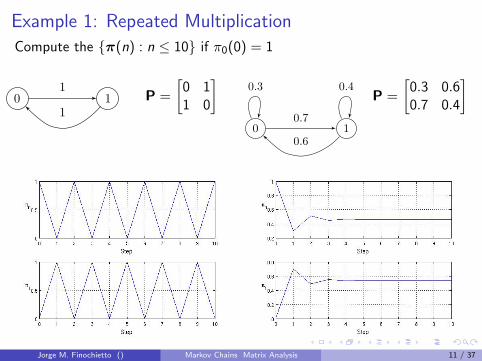
Example 1: Repeated Multiplication

Compute the {π(n) : n ≤ 10} if π0(0) = 1

0 11

1P =

[0 11 0

]0 1

0.3

0.7

0.4

0.6

P =

[0.3 0.60.7 0.4

]


MATLAB Exercise

1 Define an initial condition vector s(0)2 Compute the distribution vector for a specific n

I MATLAB function: Pns(0)

3 Compute the distribution vectors from 0 to nI Repeated multiplication: MATLAB function state vs time(P, s(0), n)

4 Plot the distribution vector evolutionI MATLAB function: plot state vs time(P, s(0), n)


Diagonalizing P

By definition the eigenvectors satisfy the following relation

Pxi = λixi

PX = XD

where D is the diagonal matrix whose diagonal elements are theeigenvalues of P

D =

λ1 0 . . . 00 λ2 . . . 0. . . . . . . . . . . .0 0 . . . λm

Thus, P can be expressed as

P = XDX−1


Diagonalizing Pn

Then Pn can be computed as follows

Pn = (XDX−1)× XDX−1 × . . .× XDX−1

Pn = XDnX−1

Since D is a diagonal matrix, Dn can be computed

D =

λn

1 0 . . . 00 λn

2 . . . 0. . . . . . . . . . . .0 0 . . . λn

m

Thus, π(n) can be expressed as

π(n) = XDnX−1π(0)


MATLAB Exercise

1 Compute the distribution vector for a specific nI First, MATLAB function: [XD] = eig(P)I Then, π(n) = XDnX−1s(0)


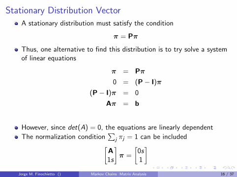
Stationary Distribution Vector

A stationary distribution must satisfy the condition

π = Pπ

Thus, one alternative to find this distribution is to try solve a systemof linear equations

π = Pπ

0 = (P− I)π

(P− I)π = 0

Aπ = b

However, since det(A) = 0, the equations are linearly dependent

The normalization condition∑

j πj = 1 can be included[A1s

]π =

[0s1

]Jorge M. Finochietto () Markov Chains Matrix Analysis 16 / 37

Example 2

Compute the stationary distribution π

0 11

1P =

[0 11 0

]0 1

0.3

0.7

0.4

0.6

P =

[0.3 0.60.7 0.4

]

π = {0.5, 0.5} π = {0.4615, 0.5385}


MATLAB Exercise

1 Compute the stationary distribution for PI First, MATLAB: stationary lineq.m


Expanding Pn

We can expand Pn in terms of its eigenvalues

Pn = XDnX−1

Pn = λn1A1 + λn

2A2 + . . .+ λnmAm

We assume that λ1 = 1

Pn = A1 + λn2A2 + . . .+ λn

mAm

More in details

Pn = λn1X

1 0 . . . 00 0 . . . 0. . . . . . . . . . . .0 0 . . . 0

X−1+. . .+λnmX

0 0 . . . 00 0 . . . 0. . . . . . . . . . . .0 0 . . . 1

X−1


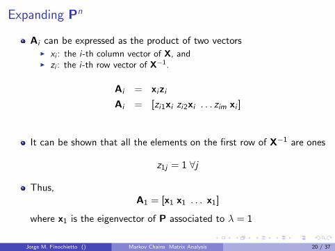
Expanding Pn

Ai can be expressed as the product of two vectorsI xi : the i-th column vector of X, andI zi : the i-th row vector of X−1.

Ai = xizi

Ai = [zi1xi zi2xi . . . zim xi ]

It can be shown that all the elements on the first row of X−1 are ones

z1j = 1 ∀j

Thus,A1 = [x1 x1 . . . x1]

where x1 is the eigenvector of P associated to λ = 1


π(n) Limiting Probabilities

Since we assume that λ1 = 1, then λi < 1 i 6= 1

Thus, as n→∞, λi → 0 i 6= 1

Pn ≈ A1 n→∞

To compute the limiting probability of π(n)

π(n) = Pnπ(0)

π(n) = [A1 + λn2A2 + . . .+ λn

mAm]π(0)

π(n→∞) = A1π(0)

π(n→∞) = [x1 x1 . . . x1]π(0)

No matter what the initial conditions are that

π(n→∞) = x1


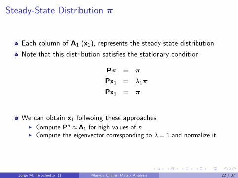
Steady-State Distribution π

Each column of A1 (x1), represents the steady-state distribution

Note that this distribution satisfies the stationary condition

Pπ = π

Px1 = λ1π

Px1 = π

We can obtain x1 follwoing these approachesI Compute Pn ≈ A1 for high values of nI Compute the eigenvector corresponding to λ = 1 and normalize it


Identifying Irreducible Aperiodic DTMC

Irreducible

Let P be the transient matrix of a DTMC whose eigenvalue λ = 1correspond to eigenvector x. Then the chain is irreducible if x has no zero

elements.

Aperiodic

Let P be the transient matrix of a DTMC with one eigenvalue λ = 1.Then all other eigenvalues muts lie inside the unit circle |λi | < 1.


MATLAB Exercise

1 Verify that the DTMC is irreducible and aperiodic.2 Compute the steady-state distribution for P

I MATLAB: Pn

I MATLAB: steady eigen.m


Mean Return Time

Recall that mean return times can be computed as follwos

Mi = E [Ti ] =∞∑

n=1

n f(n)i ∀i ∈ S

However, note that during N time steps, the chain is in state i forNi < N

Ni = N × πi

Thus, on average, the chain returned to state i every N/Ni steps

N

Ni=

1

πi

Thus, the mean return time can be expressed as

Mi =1

πi


Mean Sojourn Time

Recall that sojourn times have a geometric distribution

Pr(Wi = k) = pk−1ii (1− pii )

We can compute the mean sojourn time as follows

Si = E [Wi ] =∞∑

k=1

kpk−1ii (1− pii ) =

1

1− pii

Si =1

1− pii


Case: Transmision over Noisy Channel

An on-off source generates packets with probability a per time step.

The channel introduces errors in the packets with probability e.

If the packet has no errors, and ACK is received in the next time step.

If no ACK is received, the packet is retransmitted.

This can be modelled with a DTMC whose states areI S1: Source is idle.I S2: Source re-transmits a packet.I S3: Packet has no errors.I S4: Packet has errors.


Case: Transmision over Noisy Channel

A packet is transmitted witherrors with probability ae

A packet is transmitted with noerrors with probability a(1− e)

A packet is re-transmitted witherrors with probability e

A packet is re-transmitted withno errors with probability 1− e

P =

1− a 0 1 0

0 0 0 1a(1− e) 1− e 0 0

ae e 0 0


Exercise

For a = 0.8 and e = 0.2, compute

1 Mean retransmission time (how much time does it take to retransmita packet on average?)

2 Mean retransmission period (how much time passes on averagebetween retransmissions?)

1 A retransmission lasts multiples of 2 time steps since implies movingaround states 2 and 4. Since the probability of leaving these states is1− e), we stay with probability e. Thus, the mean retransmissiontime can be computes as 2

1−e = 2× 54 = 2.5

2 Since the probabilitie of being in either state 2 or 4 is π2 + π4, thenwe can compute the retransmission period as its inverse.


Case: CSMA/CD (Ethernet)

In carrier sense multiple access with collision detection (CSMA/CD)networks, a users access the network (i.e., transmits n packets) whenthe channel is not busy.

However, if more than one user sense that the channel is free, acollision takes place (data are lost).

When collisions are detected, the user returns to an idle state (stopstranmission).

I For simplicity, no backoff strategies are adopted.


Case: CSMA/CD (Ethernet)

We assume the following probabilitiesI u0 all users are idleI u1 only one user is transmittingI 1− u0 − u1 more than one user is

trasmitting

The channel can be in one of thesestates:

I i idle stateI t transmitting stateI c collided state


Balance Equations

In steady-state, the stationary condition π = Pπ is satisfied so wecan write

πi =∑

j

pijπj

Since the transition probability satisfies∑j

pji = 1

(the sum of all probabilities leaving state i is equal to 1(

Thus,πi

∑j

pji =∑

j

pjiπi =∑

j

pijπj

In steady-state, there must be a flow balance for each state i


Balance Equations: Finite DTMC

Compute the steady-state distribution π using balance equations

0 1

1− p

p

1− q

q

π0p = π1q

π0 + π1 = 1

π0p = π1q

π0p = q(1− π0)

π0(p + q) = q

π0 =q

p + q

π0 + π1 = 1q

p + q+ π1 = 1

π1 = 1− q

p + q

π1 =p

p + q


Exercise

Compute the steady-state distribution π using balance equations


Balance Equations: Infinite DTMC (Birth-Death Process)

Represent the current size of a population and where the transitionsare limited to births and deaths

where at each step with the probabilityI a there is a birth (arrival)I b = 1− a there is no birth (arrival)I c there is a death (departure)I d = 1− c there is no death (departure)

Thus, with probabilityI ad there is an increase in the populationI bc there is a decrease in the populationI f = ac + bd the population size is unchangedI f0 = ac + b the population is null


Infinite DTMC: Birth-Death Process

We can derive the steady-state distribution using balance equations

1)

π1bc = π0ad

π1 =

(ad

bc

)π0

2)

π2bc = π1ad

π2 =

(ad

bc

)π1 =

(ad

bc

)2

π0

πi =

(ad

bc

)i

π0

πi = ρiπ0


Infinite DTMC: Birth-Death Process

πi = ρiπ0

Next, we make us of the normalization condition∞∑i=0

πi = 1

π0

∞∑i=0

ρi = 1

π0

1− ρ = 1 if ρ < 1

π0 = 1− ρ

Thus, the steady-state distribution exists if ρ < 1

πi = ρi (1− ρ)


markov chains matrix analysis - laboratorio de ...lcd.efn.unc.edu.ar/pdf/2_matrices.pdf · 1 build...

Documents