Markovian Approaches to Joint-life Mortality

Min Ji∗

Mary Hardy†

Johnny Siu-Hang Li‡

Abstract

Many insurance products provide benefits that are contingent on the com-bined survival status of two lives. To value such benefits accurately, we requirea statistical model for the impact of the survivorship of one life on another.In this paper, we first set up two models, one Markov and one semi-Markov,to model the dependence between the lifetimes of a husband and wife. Fromthe models we can measure the extent of three types of dependence: (1) theinstantaneous dependence due to a catastrophic event that affect both lives; (2)the short-term impact of spousal death; (3) the long-term association betweenlifetimes. Then we apply the models to a set of joint-life and last-survivor an-nuity data from a large Canadian insurance company. Given the fitted models,we study the impact of dependence on annuity values, and examine the poten-tial inaccuracy in pricing if we assume lifetimes are independent. Finally, wecompare our Markovian models with two copula models considered in previousresearch on modeling joint-life mortality.

1 Introduction

Several empirical studies in recent years suggest considerable dependence between the

lifetimes of a husband and wife. Denuit et al. (2001) argue that a husband and wife

∗Min Ji is a PhD Candidate at the University of Waterloo, Waterloo, Ontario, Canada.†Mary Hardy holds the CIBC Chair in Financial Risk Management at the University of Waterloo.‡Johnny Siu-Hang Li holds the the Fairfax Chair in Risk Management at the University of

Waterloo.

1

are exposed to similar risks, since they share common lifestyles and may encounter

common disasters. Jagger and Sutton (1991) show that there is an increased relative

risk of mortality following spousal bereavement. This condition, which they call the

‘broken-heart syndrome’, can last for a prolonged period of time. It is separate from

the ‘common shock’ effect, which accounts for simultaneous deaths of a couple from a

common disaster, such as a car or airplane crash. The broken heart syndrome is used

to describe a period of higher mortality of an individual after his or her partner’s

death, even though the cause of the two deaths may appear to be independent.

We find evidence of both common shock and broken-heart effects in the data set

used in this paper. All these findings call for appropriate methods to model lifetime

dependence, which may have a significant impact on risk management for joint-life

insurance policies.

One way to model dependence between lifetimes is through copulas. Frees et

al. (1996) and Youn and Shemyakin (2001) use a Frank’s copula and a Hougaard

copula respectively to model joint-life mortality. We refer interested readers to Frees

and Valdez (1998), Klugman et al. (2008) and McNeil et al. (2005), who offer

comprehensive descriptions of copula models. An attractive advantage of the copula

approach is that it allows the correlation structure of the remaining lifetime variables

to be estimated separately from their marginal distributions. Nevertheless, by using

copulas it is implicitly assumed that the dependence structure is static over time.

Such a strong assumption may not hold true in reality. In addition, choosing a

suitable copula may not be straightforward. While we can compare one copula with

another, whether either actually fits the dependence structure adequately is not easy

to quantify, and it is rare to have a qualitative or intuitive justification for a specific

copula.

Another way to model dependence is to use finite state Markov models. Transi-

tions between states are governed by a matrix of transition intensities. Depending

on the properties of the transition intensities, models may be (fully) Markov or semi-

Markov. In Markov models, transition intensities depend on the current state only,

while in semi-Markov models, transition intensities depend on both the current state

and the time elapsed since the last transition (the sojourn time in the current state).

Markov and semi-Markov models are highly transparent, as we see clearly from the

multiple state model how a change of state, for example, from married to widowed,

impacts mortality.

2

Markov multiple state models have been applied to diverse areas in actuarial sci-

ence. Sverdrup (1965) and Waters (1984) both considered models where the states

represented different health statuses. The first application to joint-life mortality mod-

eling may be by Norberg (1989). Spreeuw and Wang (2008) extend Norberg’s work

by allowing mortality to vary with the time elapsed since death of spouse. Dickson et

al (2009) explain how finite state Markov models may be used for modelling various

insurance benefits, including joint life, critical illness, accidental death and income

replacement insurance.

This study, conducted simultaneously with that of Spreeuw and Wang (2008),

considers different extensions to Norberg’s model. First, we introduce to the model a

common shock factor, which is associated with the time of a catastrophe, for example,

a plane crash, that affects both lives. The common shock dependency between couples

is well covered in actuarial literature, following its introduction (as the ‘fatal shock’)

in Marshall and Olkin (1967). It is well described in Bowers et al (1997), in the

context of a competing risks model, and in Dickson et al (2009) in a Norberg-type

Markov multiple state model. Secondly, we extend Norberg’s original Markov model

to a semi-Markov model, which characterizes the impact of bereavement on mortality

through a smooth parametric function of the time elapsed since bereavement. The

parametric function provides more information about how the bereavement diminishes

with time than the step function given by Spreeuw and Wang (2008). Furthermore,

we offer a comparison between the multiple state and copula approaches, by applying

our models to the data set used by Frees et al. (1996) and Youn and Shemyakin

(2001).

The rest of this paper is organized as follows. Section 2 describes the data we

use throughout this study. Section 3 illustrates the concept of Markovian modeling

with a simple Markov model. Section 4 presents the full semi-Markov model with a

parametric function for modeling the broken heart effect. Detailed information about

the model structures and the estimation procedure is provided. Section 5 compares

annuity prices using the Markov model with the semi-Markov model. Section 6 com-

pares the semi-Markov model with the copulas proposed in Frees et al (1996) and in

Youn and Shemyakin (2001). Section 7 concludes the paper.

3

2 The data

The data used in this paper were developed in the research reported in Frees et al

(1996), funded by the Society of Actuaries. Youn and Shemyakin (2001) as well as

Spreeuw and Wang (2008) also used this data. The data set contains 14,947 records of

joint and last-survivor annuity contracts, over an observation period from December

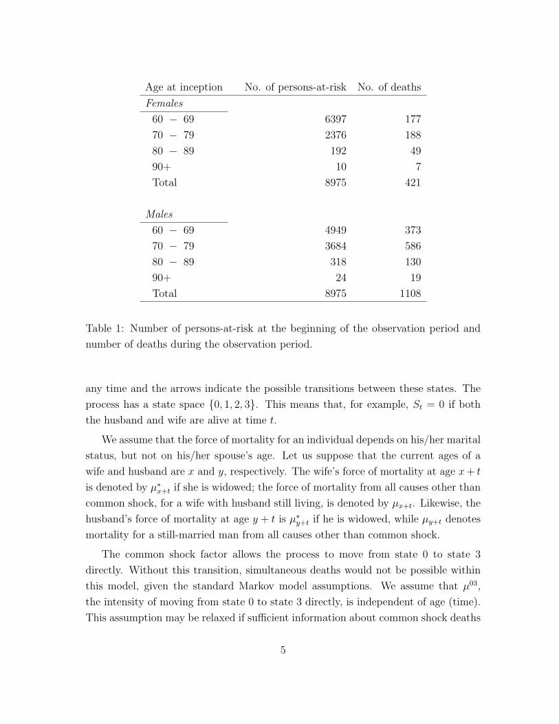
29, 1988 to December 31, 1993. In Table 1 we show a summary of the data after

the removal of replicated records and records associated with annuitants of the same

sex. It is interesting to note that the death counts for males are almost three times

that for females. This observation implies that there is significantly more information

about widowed females than widowed males.

In Table 2 we show the breakdown of the data by the following categories: (1)

survived to the end of the observation period; (2) died at least 5 days before or after

spouse’s death; (3) died within 5 days before or after spouse’s death. As we aim to

model separately the impact of a ‘common shock’, and the impact of bereavement on

the widow(er)’s physiognomy, we use a common shock transition in the Markovian

models, which we assume to include cases where partners die within 5 days of each

other. The use of a 5-day cut-off to allocate the deaths to common shock is admittedly

somewhat arbitrary. The issues are discussed and analysed further in Section 4.

We encourage those collecting data to include a notation when deaths arise from a

common cause, to avoid this uncertainty in future applications.

3 Markov model

3.1 Model specification

Before we present our extension to Norberg’s (1989) work, we illustrate the concept

of multiple-state modeling with a simple Markov model.

A stochastic process {St, t ≥ 0} is a Markov process if, for any u > v > 0, the

conditional probability distribution of Su, given the whole history of the process up

to and including time v, depends on the value of Sv only. In other words, given Sv,

the process at time u is independent of the history of the process before time v.

The Markov process for this study can conveniently be represented by the diagram

in Figure 1. The boxes represent the four possible states that a couple can be in at

4

Age at inception No. of persons-at-risk No. of deaths

Females

60 − 69 6397 177

70 − 79 2376 188

80 − 89 192 49

90+ 10 7

Total 8975 421

Males

60 − 69 4949 373

70 − 79 3684 586

80 − 89 318 130

90+ 24 19

Total 8975 1108

Table 1: Number of persons-at-risk at the beginning of the observation period and

number of deaths during the observation period.

any time and the arrows indicate the possible transitions between these states. The

process has a state space {0, 1, 2, 3}. This means that, for example, St = 0 if both

the husband and wife are alive at time t.

We assume that the force of mortality for an individual depends on his/her marital

status, but not on his/her spouse’s age. Let us suppose that the current ages of a

wife and husband are x and y, respectively. The wife’s force of mortality at age x+ t

is denoted by µ∗x+t if she is widowed; the force of mortality from all causes other than

common shock, for a wife with husband still living, is denoted by µx+t. Likewise, the

husband’s force of mortality at age y + t is µ∗y+t if he is widowed, while µy+t denotes

mortality for a still-married man from all causes other than common shock.

The common shock factor allows the process to move from state 0 to state 3

directly. Without this transition, simultaneous deaths would not be possible within

this model, given the standard Markov model assumptions. We assume that µ03,

the intensity of moving from state 0 to state 3 directly, is independent of age (time).

This assumption may be relaxed if sufficient information about common shock deaths

5

Females Males

Survived 8635 7924

Died within 5 days of spouse’s death 52 52

Died at least 5 days before/after spouse’s death 288 999

Total 8975 8975

Table 2: Breakdown of the data by survival status at the end of the observation

period.

State 0 State 1Husband deadWife alive

x 03 x*

State 2 State 3Wife deadHusband alive

y

y*

Both alive

Both dead

Figure 1: Specification of the Markov model.

is available. The use of the common shock transition means that the total force of

mortality for a married woman age x + t is µx+t + µ03, and similarly for a married

man (Bowers et al (1997)).

In many applications of the model, we require the following transition probabili-

ties:

tpijx = Pr(Sx+t = j|Sx = i), i, j = 0, 1, 2, 3, x, t ≥ 0.

The computation of these probabilities requires two technical assumptions, in

addition to the Markov assumption. Assumption (1): the probability of two or

more transitions in a small interval h is o(h), where o(.) is a function such that

limh→0 o(h)/h = 0. Assumption (2): tpijx is a differentiable function of t. Given these

two assumptions, we can compute tpijx by the Kolmogorov forward equations, which

6

can be written in a compact form as

∂

∂tP (x, x+ t) = P (x, x+ t)A(x+ t), x, t ≥ 0,

where P (x, x+t) is a matrix in which the (i, j)th entry is tpijx , i, j = 1, 2, 3 and A(x+t)

is called the infinitesimal generator matrix, also known as the intensity matrix. The

(i, j)th element is µijx+t for i 6= j, and −∑3

j=0,j 6=i µij(x + t) for i = j. Solving this

system of partial differential equations, we obtain the following expressions for the

transition probabilities:

tp00x:y = exp

(−∫ t

0

µx+s + µy+s + µ03 ds)

;

tp11x = exp

(−∫ t

0

µ∗x+s ds)

;

tp01x:y =

∫ t

0sp

00x:y µy+s t−sp

11x+s ds;

tp02x:y =

∫ t

0sp

00x:y µx+s t−sp

22y+s ds;

tp13x =

∫ t

0sp

11x µ∗x+s ds;

tp23y =

∫ t

0sp

22y µ∗y+s ds.

See Dickson et al (2009) for details.

3.2 Parameter estimation

Let Tx and Ty be the remaining lifetimes of a wife and husband, respectively. The

joint density function for Tx and Ty can be loosely expressed as

fTx,Ty(u, v) =

{up

00x:y v−up

22y+u µx+u µ

∗y+v, if u < v,

vp00x:y u−vp

11x+v µy+v µ

∗x+u, if u > v,

(1)

fTx,Ty(u, u) = up00x:y µ

03

7

Given the joint density function, we can construct the log-likelihood function from

which maximum likelihood estimates of transition intensities can be derived. Assum-

ing independence among different couples in the data, the log-likelihood function can

be written as a sum of three separate parts, `1, `2, and `3, where

`1 =n∑i=1

(−∫ vi

0

(µxi+t + µyi+t + µ03) dt+ d1i lnµyi+vi

+ d2i lnµxi+vi

+ d3i lnµ03

),

`2 =

m1∑j=1

(−∫ u1,j

0

µ∗xj+t dt+ h1,j lnµ∗xj+u1,j

),

`3 =

m2∑k=1

(−∫ u2,k

0

µ∗yk+t dt+ h2,k lnµ∗yk+u2,k

),

where

• n is the total number of couples in the data set,

• m1 (m2) is the total number of widows (widowers) in the data set,

• vi is the time until the ith couple exits state 0, i = 1, ..., n,

• dji = 1 if the the ith couple moves from state 0 to state j at t = vi, i = 1, ..., n,

j = 1, 2, 3,

• u1,j (u2,k) is the time until the jth (kth) widow (widower) exits state 1 or 2,

j = 1, ...,m1, k = 1, ...,m2,

• h1,j = 1 if the jth widow dies at t = u1,j,

• h2,j = 1 if the kth widower dies at t = u2,k,

• xi and yi are the entry ages of the wife and husband of the ith couple, respec-

tively.

By maximizing three parts of log-likelihood function separately, we can get the

maximum likelihood estimates of the transition intensities in each state. Note that,

for right censored data, dji , h1,j, and h2,j will be zero.

To calculate the log-likelihood, there is a need to define ‘common shock’ deaths.

As we do not have cause of death information which would give definitive information

8

on this point, we treat the 52 deaths which occurred within 5 days before or after

bereavement as simultaneous deaths. A deeper discussion of the five day threshold is

provided in Section 4 in which we present the full semi-Markov model.

Although one could assume that the forces of mortality are piecewise constant, in

this study we graduate the forces of mortality (except µ03, which is assumed to be

invariant with age) using Gompertz’ law, µx = BCx. The parametric graduation is

used because it is parsimonious, it allows us to extrapolate the forces of mortality to

extreme ages, it smooths the results, and it enables us to calculate quantities such

as annuity values efficiently. Although we use the Gompertz model, we do not claim

that it provides the best fit of all possible models. Our point here is to illustrate the

combination of the individual mortality model (Gompertz, for simplicity) with the

multiple state model overlay which provides the dependency framework.

Assuming then, that for both sexes, mortality in state 0 follows Gompertz’ law,

we can rewrite `1 as

`1 =n∑i=1

(−B1C

yi1 (Cvi

1 − 1)

ln(C1)+ d1

i ln(B1Cyi+vi1 )− B2C

xi2 (Cvi

2 − 1)

ln(C2)

+d2i ln(B2C

xi+vi2 )− viµ03 + d3

i ln(µ03)),

(2)

where (B1, C1) and (B2, C2) are the Gompertz parameters for female and male mor-

tality in state 0, respectively. We can rewrite `2 and `3 in a similar manner. The

maximum likelihood estimate of µ03 is 0.1407%, and its standard error is 0.0195%.

Maximum likelihood estimates of other parameters are displayed in Table 3. Param-

eters µ∗x and µ∗y have higher standard errors, since the number of individuals who

transition to states 1 or 2 is relatively small (see Table 2), even in this extensive data

set.

In Figure 2 we plot the fitted forces of mortality in different states. We observe,

for both sexes, an increased force of mortality after bereavement, after allowing for

common cause deaths using the 5-day common shock allocation. We can further

observe from Figure 2 that bereavement effects vary with age, as the mortality curves

do not shift in parallel.

Common cause deaths with more than 5 days between events could be the cause

of the increase in mortality post-bereavement; however, as we demonstrate in Figure

3, the impact is fairly long-lasting, increasing the possibility that the bereavement

impact is not solely caused by common shock mortality. Figure 3 shows, for both

9

B Standard error C Standard error

Females

µx 9.741× 10−7 2.889× 10−7 1.1331 0.0047

µ∗x 2.638× 10−5 3.370× 10−5 1.1020 0.0181

Males

µy 2.622× 10−5 1.038× 10−5 1.0989 0.0058

µ∗y 3.899× 10−4 4.057× 10−4 1.0725 0.0136

Table 3: Estimates of Gompertz parameters in the Markov model.

60 70 80 900

0.02

0.04

0.06

0.08

0.1

0.12

0.14

0.16

0.18

Age

For

ce o

f Mor

talit

y

Female

60 70 80 900

0.05

0.1

0.15

0.2

0.25

Age

For

ce o

f Mor

talit

y

Male

μx*

μx + μ03

μy*

μy + μ03

Figure 2: Forces of mortality by marital status (married or widowed)

10

60 70 80 900

0.05

0.1

0.15

0.2

0.25

0.3

0.35

Age

For

ce o

f Mor

talit

y

Female

μ*x|0

μ*x|1

μ*x|2+

60 70 80 900

0.05

0.1

0.15

0.2

0.25

0.3

0.35

Age

For

ce o

f Mor

talit

y

Male

μ*y|0

μ*y|1

μ*y|2+

Figure 3: Force of mortality by period since bereavement; µ∗x(y)|0 in first year, µ∗x(y)|1

in second year, µ∗x(y)|2+ after the second year.

sexes, the graduated values of the following three forces of mortality:

• µ∗x(y)|0: the force of mortality during the first year after bereavement;

• µ∗x(y)|1: the force of mortality during the second year after bereavement;

• µ∗x(y)|2+ : the force of mortality beyond the second year after bereavement.1

To examine whether the Gompertz’ laws give an adequate fit, we perform a χ-

square test. For µx, µ∗x and µ∗y, the null hypothesis that model gives an adequate fit

is not rejected at 5% level of significance, but for µy, the null hypothesis is marginally

rejected (the p-value is 0.042). The fit for µy can be improved by using Makeham’s

law, µx = A + BCx, which increases the p-value for the χ-square to 0.13, indicating

an adequate fit. However, for consistency reasons, we use Gompertz’ law for all four

forces of mortality, even though Makeham’s law may better fit µy.

As we have stated, the Gompertz model is used mainly for illustration, and this

test is simply to ensure that the model is not radically out of line with the data.

1In calculating these forces of mortality, we treat deaths which occurred within 5 days before orafter bereavement as simultaneous deaths. The graduation is based on Gompertz law.

11

Alternative models, for example, non-parametric Kaplan-Meier estimates, can also

be used. However, because of very sparse data at high ages, Kaplan-Meier and other

non-parametric approaches have drawbacks. We reiterate that, our purpose is more

to demonstrate the methodology than to give definitive answers. We encourage inter-

ested readers to apply their own data sets and determine the models most appropriate

to them.

4 The Semi-Markov Model

4.1 Model specification

The Markov model described above is somewhat rigid, in that the bereavement effect

(other than common cause) is assumed to be constant, regardless of the length of time

since the spouse’s death. While it might be reasonable that mortality of widow(er)s is

generally higher than married individuals of the same age, it also seem reasonable to

consider that the detrimental impact of bereavement on the surviving spouse’s health

might be stronger in the months immediately following the spouse’s death than it

is later on. In fact, the medical and demographic descriptions of the broken heart

syndrome generally measure this shorter term impact (Jagger and Sutton, 1991).

Figure 3 indicates that the bereavement mortality dynamics depend on the pe-

riod since bereavement, which implies that a semi-Markov approach might better

capture the dynamics. We observe that, at any given age, mortality is highest in the

year following widow(er)hood, and lowest two years later. We should caution that,

even though the data set is very large, the individual counts by age and time since

widow(er)hood are sparse at most ages. The graduated data support the semi-Markov

model, but there is clearly significant uncertainty.

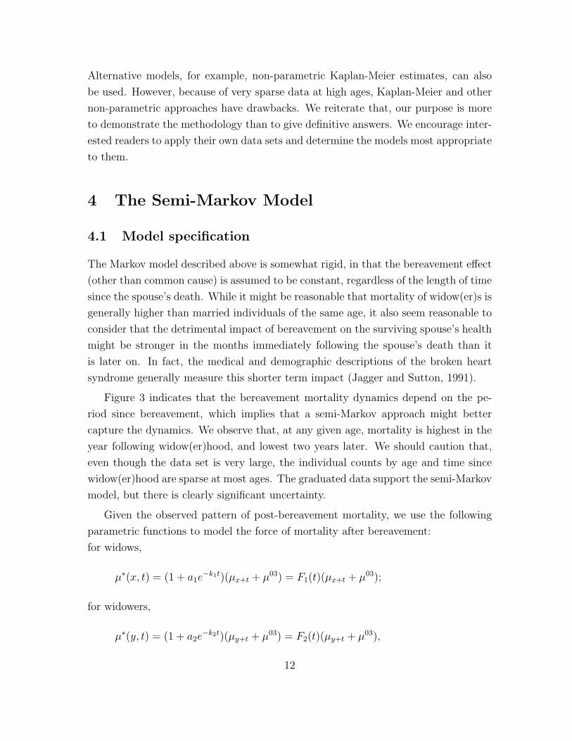
Given the observed pattern of post-bereavement mortality, we use the following

parametric functions to model the force of mortality after bereavement:

for widows,

µ∗(x, t) = (1 + a1e−k1t)(µx+t + µ03) = F1(t)(µx+t + µ03);

for widowers,

µ∗(y, t) = (1 + a2e−k2t)(µy+t + µ03) = F2(t)(µy+t + µ03),

12

State 0 Both are alive

State 2 Wife is dead,

husband is alive

State 1 Husband is dead,

wife is alive

State 3 Both are dead

μ03 μ*(x,t)

μ*(y,t)

μy

μx

Figure 4: Specification of the semi-Markov model

where t is the time since bereavement. Under this model, the force of mortality after

bereavement is proportional to the corresponding force of mortality if bereavement

did not occur. Initially, bereavement increases the force of mortality by a percentage

of 100a1% for females and 100a2% for males. As t increases, the multiplicative factors

F1(t) = 1+a1e−k1t and F2(t) = 1+a2e

−k2t decrease exponentially and finally approach

1, capturing the selection effect on the broken-heart syndrome. Parameters k1 and k2

govern the speed at which the selection effect diminishes. The complete specification

of the semi-Markov model is shown diagrammatically in Figure 4.

4.2 Parameter estimation

Because the semi-Markov extension affects post-bereavement mortality only, there is

no change to the meaning and values of µx, µy, and µ03. Given the estimates of µx, µy,

and µ03, the remaining parameters can be estimated by partial maximum likelihood

estimation. The partial likelihood function `p1 for parameters a1 and k1 is given by

`p1 =

m1∑j=1

(−∫ u1,j

0

(1 + a1e−k1t)(B1C

x+t1 + µ03)dt (3)

+h1,j ln(

(1 + a1e−k1t)(B1C

x+t1 + µ03)

)),

13

where B1 and C1 are the maximum likelihood estimate for B1 and C1, respectively

(see Table 3). The partial likelihood function `p2 for a2 and k2 can be obtained by

changing the parameters in `p1 accordingly. By maximizing `p1 and `p2, we can obtain

estimates for the semi-Markov parameters.

The estimates of a1, a2, k1, and k2 and their approximate standard errors are

shown in Table 4. The standard errors in Tables 3 and 4 are estimated using numerical

approximation of the second derivative of the likelihood function. They do not allow

for the dependence between the parameter estimates; a more accurate assessment

could be obtained using Bayesian or bootstrap techniques. A limitation of the semi-

Markov model is high parameter uncertainty, because the parameters are estimated

from a small number of post-bereavement deaths. Nevertheless, the estimates indicate

the need for both the for the magnitude terms, aj and decay terms, kj.

Central estimate Standard error

Females

a1 3.3845 0.9164

k1 0.5216 0.2468

Males

a2 11.0530 4.5080

k2 7.9070 3.2293

Table 4: Estimates of parameters a1, a2, k1, and k2 in the semi-Markov model

Figure 5 displays how the multiplicative factors F1(t) and F2(t) vary with time.

The upper panel, which focuses on the first year after bereavement, shows that wid-

owers are subject to a much higher broken heart effect shortly after bereavement.

However, as the lower panel indicates, the broken heart effect for widows is more

persistent than that for widowers.

Since µ∗x and µ∗y in the semi-Markov model are functions of both age (x) and time

since bereavement (t), conducting a chi-square test for each specific force of mortality

(as in Section 3) would require us to group the deaths not only by x but also by t. In

such a grouping, the number of deaths in each group will not be significant enough

for us to perform the test with sufficient granularity.

14

0 0.5 10

1

2

3

4

5

0 ≤ t ≤ 1F

1(t)

Female

0 0.5 10

2

4

6

8

10

12

0 ≤ t ≤ 1

F2(t

)

Male

0 5 100

1

2

3

4

5

0 ≤ t ≤ 10

F1(t

)

0 5 100

2

4

6

8

10

12

0 ≤ t ≤ 10

F2(t

)

Figure 5: Factors F1(t) and F2(t) in the semi-Markov model.

4.3 Identifying common shock deaths

In the semi-Markov model, the following two separate effects are explicitly modeled:

1. the impact in the first five days, where we assume that deaths are simultaneous

using the common shock approach. This is used to model a catastrophic event

causing the proximate deaths of both partners. We have also called this the

common cause effect, and this is identical to the ‘fatal shock’ of Marshall and

Olkin (1967).

2. the impact after the first five days, which we have termed the bereavement or

broken-heart effect.

We could build the common shock deaths into the semi-Markov model without the

µ03 transitions, but the semi-Markov functions would be more complex, requiring a

probability mass at t = 0 followed by the decaying factors. The separation of the two

bereavement effects seems to us more transparent and intuitive, especially considering

that the common shock model is already well known to many actuaries. In building

the model though, the threshold for defining simultaneous deaths is important, par-

ticularly if our aim is to separate common-cause impact from broken-heart impact. If

15

the threshold is set too long, some deaths associated with the broken-heart effect will

be misclassified as simultaneous deaths, leading to an overestimation of µ03. If the

threshold is set too short, some simultaneous deaths will be misclassified, affecting

the shape of the multiplicative factors F1(t) and F2(t), which are intended to model

the broken-heart and not the common shock effect. These functions become heavily

skewed to account for the very short term impact, if distorted by common shock data,

as we show below.

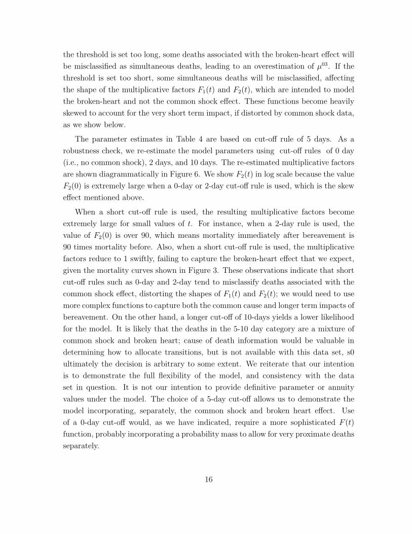
The parameter estimates in Table 4 are based on cut-off rule of 5 days. As a

robustness check, we re-estimate the model parameters using cut-off rules of 0 day

(i.e., no common shock), 2 days, and 10 days. The re-estimated multiplicative factors

are shown diagrammatically in Figure 6. We show F2(t) in log scale because the value

F2(0) is extremely large when a 0-day or 2-day cut-off rule is used, which is the skew

effect mentioned above.

When a short cut-off rule is used, the resulting multiplicative factors become

extremely large for small values of t. For instance, when a 2-day rule is used, the

value of F2(0) is over 90, which means mortality immediately after bereavement is

90 times mortality before. Also, when a short cut-off rule is used, the multiplicative

factors reduce to 1 swiftly, failing to capture the broken-heart effect that we expect,

given the mortality curves shown in Figure 3. These observations indicate that short

cut-off rules such as 0-day and 2-day tend to misclassify deaths associated with the

common shock effect, distorting the shapes of F1(t) and F2(t); we would need to use

more complex functions to capture both the common cause and longer term impacts of

bereavement. On the other hand, a longer cut-off of 10-days yields a lower likelihood

for the model. It is likely that the deaths in the 5-10 day category are a mixture of

common shock and broken heart; cause of death information would be valuable in

determining how to allocate transitions, but is not available with this data set, s0

ultimately the decision is arbitrary to some extent. We reiterate that our intention

is to demonstrate the full flexibility of the model, and consistency with the data

set in question. It is not our intention to provide definitive parameter or annuity

values under the model. The choice of a 5-day cut-off allows us to demonstrate the

model incorporating, separately, the common shock and broken heart effect. Use

of a 0-day cut-off would, as we have indicated, require a more sophisticated F (t)

function, probably incorporating a probability mass to allow for very proximate deaths

separately.

16

0 1 2 3 4 51

2

3

4

5

6

7

8

0 ≤ t ≤ 5

F1(t

)

10−day5−day2−day0−day

0 0.5 1 1.5 20

1

2

3

4

5

6

0 ≤ t ≤ 2

ln[F

2(t)]

10−day5−day2−day0−day

Figure 6: Multiplicative factors F1(t) and F2(t) (in log scale) on the basis of different

cut-off rules for simultaneous deaths.

4.4 Positive Quadrant Dependence

Positive quadrant dependence (PQD) is a form of dependence between random vari-

ables X and Y , such that

Pr[(X, Y ) > (x, y)] ≥ Pr[X > x] Pr[Y > y]

or, equivalently Pr[(X, Y ) ≤ (x, y)] ≥ Pr[X ≤ x] Pr[Y ≤ y]

which means that low values of X are associated with low values of Y , and high

values of X with high values of Y . Norberg(1989) showed that for a Markov model

(with no common shock transition), the future lifetimes of the spouses, Tx and Ty are

PQD if µx ≤ µ∗x and µy ≤ µ∗y; if the forces of mortality before and after bereavement

are equal for both partners (and there is no common shock transition possible) then

the future lifetimes are independent.

PQD is relevant for actuarial calculations because, for annuities for example, a

strictly PQD model will always generate higher joint life annuity values, and lower

last survival annuity values, than an independent model. Clearly, strict PQD implies

that (in standard actuarial notation) tpxy > tpx tpy, and the joint life annuity value for

17

the dependent lives, say aPQDxy will be greater than the annuity value for independent

lives, say aIxy as

aPQDxy =

∫ ∞0

tpxye−δ tdt >

∫ ∞0

tpx tpye−δ tdt = aIxy

Similarly, (in standard actuarial notation) under PQD tqxy > tqx tqy, and the last

survivor annuity value for the dependent lives, say aPQDxy will be less than the annuity

value for independent lives, say aIxy as

aPQDxy =

∫ ∞0

(1− tqxy) e−δ tdt ≤

∫ ∞0

(1− tqx tqy) e−δ tdt = aIxy

For the fully Markov model with common shock transitions, Jie(2010) shows that

the PQD result applies, provided that

µx + µ03 ≤ µ∗x; and µy + µ03 ≤ µ∗y.

However, interestingly, under the semi-Markov model, even though the inequality

µx + µ03 ≤ µ∗x always holds, without the Markov assumption, PQD does not hold.

The reason is that under the semi-Markov framework, some spouses have time to

recover. Consider two widows, both age x. The first was widowed long ago, the

second recently. PQD requires that the mortality of the first is higher than the second,

because PQD implies that for any (t, s), Pr[Tx > t|Ty ≤ s] ≤ Pr[Tx > t|Ty > s]; that

is, that mortality of the wife is worst when the husband dies young. However, under

the semi-Markov model, the temporary increase in the force of mortality for the new

widow may increase her mortality above that of the long time widow, who has at

least partially recovered. For full details see Ji(2010).

5 Examples: last survivor annuity values

Both the Markov and semi-Markov models indicate an increase in mortality after

bereavement. However, the persistency is different. While the semi-Markov model

allows (at least partial) recovery from bereavement, the Markov model assumes that

the increase in mortality is permanent. Such a difference has an impact on annuity

values, as we now discuss.

First, let us consider the Markov model in Section 3. The three-dimensional plot

in Figure 7 shows the ratios of last survivor annuity values using the Markov-model,

18

6065

7075

8085

90

60

70

80

900.7

0.75

0.8

0.85

0.9

0.95

Male AgeFemale Age

Ann

uity

Rat

io

Figure 7: Three-dimensional plot of the ratios of Markov-model-based to independent

last-survivor annuity values (5% interest is assumed).

to values assuming independent lifetimes. All ratios in the plot are less than 1 (as we

expect from the PQD findings) confirming that last-survivor annuities are overpriced

if the assumption of independent lifetimes is used, compared with the Markov model.

We also observe that the annuity ratios are lower when the gap between the spouses’

ages is larger. This observation implies the effect of long-term dependence is more

significant when the age gap |x− y| is wider.

The three-dimensional plot in Figure 7 is clearly asymmetric. This asymmetry

can be explained by the ratios µ∗x/(µx + µ03) and µ∗y/(µy + µ03). From Figure 8 we

observe that, the ratios are different from each another, indicating a sex differential

in the effect of bereavement on mortality. Such a differential explains why we observe

an asymmetry in the plot of annuity ratios.

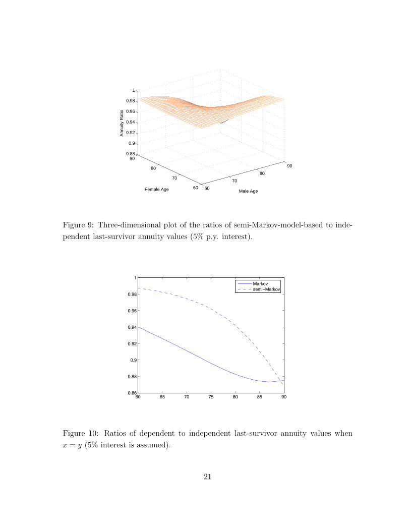
Next we consider the semi-Markov model from Section 4. Figure 9 plots the ratio

of the last-survivor annuity values using the semi-Markov model to those based on

the assumption of independence. We observe that these ratios are closer to 1.0; a

little lower at most age combinations. We also note that the plot is asymmetric, as

we would expect, given the different patterns for males and females of the impact

and likelihood of bereavement. Although all the values shown are less than 1.0, it is

possible for the ratio to exceed 1.0 for certain age combinations, unlike the Markov

19

60 65 70 75 80 85 901

2

3

4

5

6

7

8

9

Age

Rat

io

FemaleMale

Figure 8: Ratios µ∗x/(µx + µ03) and µ∗y/(µy + µ03) computed from the fitted Markov

model.

case, where PQD requires all ratios for last survivor annuity values to be less than

1.0.

For many annuity contracts, the difference between the ages of a husband and wife

is small. We found from our data set that more than 50% of the annuity contracts

are sold to couples with an (absolute) age difference of less than 2 years. So the

annuity ratios when x and y are close to each other are of particular importance. In

Figure 10 we plot the annuity ratios for x = y, on the basis of both Markov and semi-

Markov models. The Markov model results in lower annuity values for younger ages,

and higher for more advanced ages, compared with the semi-Markov model. This

can be explained by the fact that the semi-Markov model generates higher mortality

immediately after bereavement, compared with the Markov model, but later, after a

period of recovery, the ultimate rates are lower for widows and widowers under the

semi-Markov model. For younger lives, the long term mortality has more impact,

so the last survivor may be assumed to live longer, compared with the Markov,

so the annuity values are higher. For older lives, the shorter term mortality is more

significant as there is no time for long term recovery after bereavement, before extreme

old age, and so the last survivor under the semi-Markov model will have heavier overall

mortality, resulting in lower annuity values.

20

60

70

80

90

60

70

80

900.88

0.9

0.92

0.94

0.96

0.98

1

Male AgeFemale Age

Ann

uity

Rat

io

Figure 9: Three-dimensional plot of the ratios of semi-Markov-model-based to inde-

pendent last-survivor annuity values (5% p.y. interest).

60 65 70 75 80 85 900.86

0.88

0.9

0.92

0.94

0.96

0.98

1Markovsemi−Markov

Figure 10: Ratios of dependent to independent last-survivor annuity values when

x = y (5% interest is assumed).

21

6 Markovian models vs. copulas

Another way to model the dependence between the lifetimes of a husband and wife

is to use copulas. A copula C(u, v) is a bivariate distribution function over the unit

square with uniform marginals. It allows us to construct bivariate distributions for

random variables with known marginal distributions. To illustrate, let us consider

two variables X and Y with known marginal distribution functions FX(x) and FY (y),

respectively. From C(u, v) and the marginal distribution functions, we can create a

bivariate distribution function

FX,Y (x, y) = C(FX(x), FY (y)),

which introduces a degree of association between the two random variables. A good

general introduction to copulas can be found in Frees and Valdez (1998), Klugman

et al. (2008) and McNeil et al. (2005).

The use of copulas to model the dependence between two lifetimes has been con-

sidered by Frees et al. (1996) and Youn and Shemyakin (2001). Given that their

studies are based on the same data as we use in this paper, a comparison between

their and our findings may offer us some insights into how Markovian approaches are

different from copula approaches.

Frees et al. (1996) model the dependence between the lifetimes of a wife and a

husband by a Frank’s copula, which can be expressed as follows:

C(u, v) =1

αln(

1 +(eαu − 1)(eαv − 1)

eα − 1

),

where the α is a parameter that controls the degree of association between the two

random variables. Values of α less than 1 indicate a positive association, values

greater than 1 indicate an inverse interaction, and 1 indicates independence. This

copula is symmetric, because C(u, v) = C(v, u).

Using the estimation procedure provided by Frees et al. (1996), we obtain α =

−3.64. The extent of dependence between the two marginal lifetime distributions

can be measured by Kendall’s τ , which ranges from −1 and 1. We found that the

Kendall’s τ statistic for this model is 0.36, which indicates a moderate dependence

between the two marginal distributions.

On the basis of this copula, we plot in Figure 11 the ratios of dependent to

independent last-survivor annuity values for a range of ages. There are two significant

22

60

70

80

90

60

70

80

900.8

0.9

1

1.1

1.2

Male AgeFemale Age

Ann

uity

Rat

io

Figure 11: Ratios of last-survivor annuity values based on a Frank’s copula to last-

survivor annuity values based on the independent assumption (5% interest is as-

sumed).

differences between this plot and the plots based on our Markovian models. First,

this plot is roughly symmetric, which means that the marginal distributions of males’

and females’ lifetimes have approximately the same effect on the ratios. Second, the

range of ratios is much greater than for the semi-markov model, indicating a much

greater impact on the last survivor annuity value of the dependence model.

Youn and Shemyakin (2001) consider a Hougaard copula,2 which can be written

as follows:

C(u, v) = exp(−((− lnu)θ + (− ln v)θ)1/θ),

where θ ≥ 1 is a parameter that indicates the extent of dependence. When θ = 1,

there is no dependence; and when θ → ∞, the two underlying random variables

tend to be perfectly correlated with each other. This copula is also symmetric as

C(u, v) = C(v, u). Fitting a Hougaard copula to the annuitants’ mortality data, we

obtain θ = 1.57. The Kendall’s τ statistic for this model is 0.36, as for the Frank’s

copula.

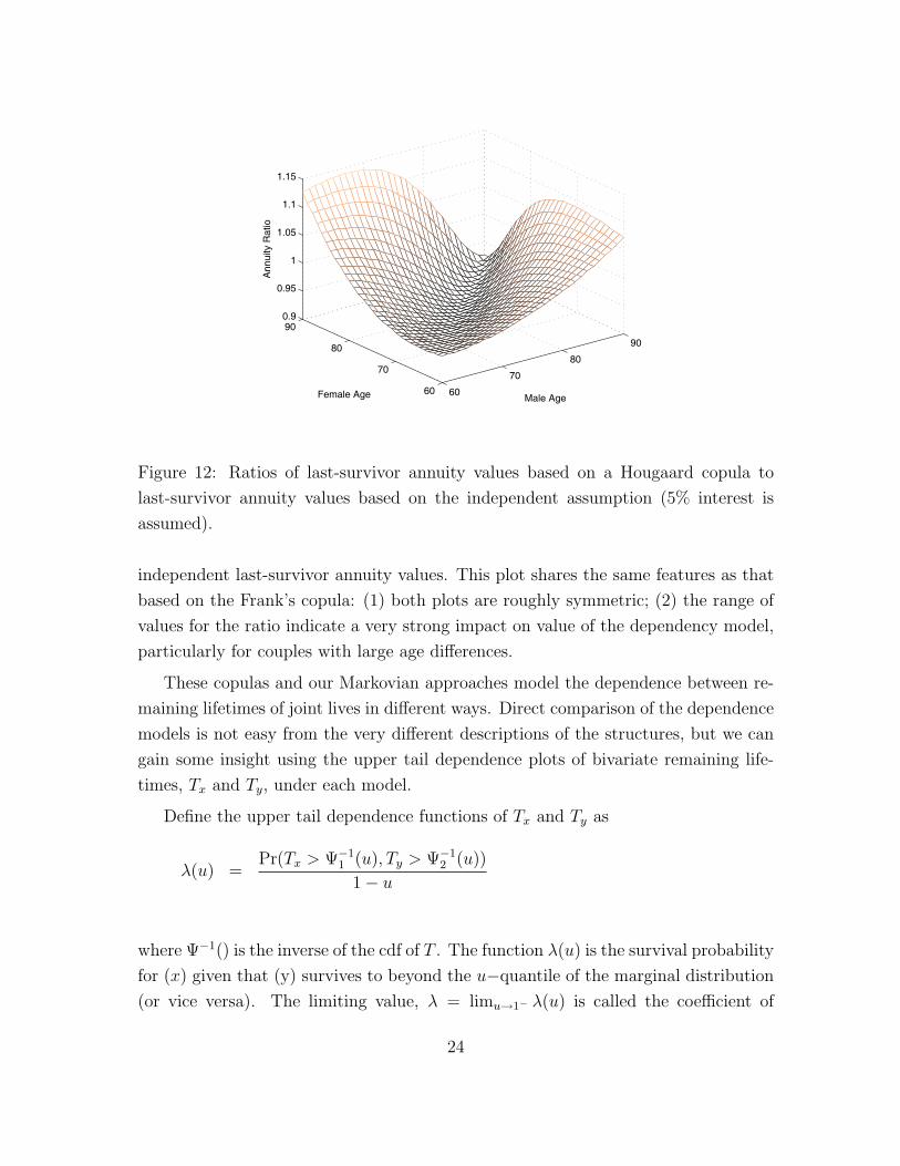
Given the Hougaard copula, we plot in Figure 12 the ratios of dependent to

2Also known as a Gumbel copula.

23

60

70

80

90

60

70

80

900.9

0.95

1

1.05

1.1

1.15

Male AgeFemale Age

Ann

uity

Rat

io

Figure 12: Ratios of last-survivor annuity values based on a Hougaard copula to

last-survivor annuity values based on the independent assumption (5% interest is

assumed).

independent last-survivor annuity values. This plot shares the same features as that

based on the Frank’s copula: (1) both plots are roughly symmetric; (2) the range of

values for the ratio indicate a very strong impact on value of the dependency model,

particularly for couples with large age differences.

These copulas and our Markovian approaches model the dependence between re-

maining lifetimes of joint lives in different ways. Direct comparison of the dependence

models is not easy from the very different descriptions of the structures, but we can

gain some insight using the upper tail dependence plots of bivariate remaining life-

times, Tx and Ty, under each model.

Define the upper tail dependence functions of Tx and Ty as

λ(u) =Pr(Tx > Ψ−1

1 (u), Ty > Ψ−12 (u))

1− u

where Ψ−1() is the inverse of the cdf of T . The function λ(u) is the survival probability

for (x) given that (y) survives to beyond the u−quantile of the marginal distribution

(or vice versa). The limiting value, λ = limu→1− λ(u) is called the coefficient of

24

0.9 0.95 10

0.1

0.2

0.3

0.4

uλ(

u)

Frank’s copula

0.9 0.95 10.47

0.48

0.49

0.5

0.51

0.52

u

λ(u)

Hougaard copula

0.9 0.95 10

0.1

0.2

0.3

0.4

u

λ(u)

Markov model

0.9 0.95 10

0.02

0.04

0.06

0.08

u

λ(u)

Semi−Markov model

Figure 13: Estimates of upper tail dependence functions λ(u)

the upper tail dependence, if it exists. If λ = 0, then Tx and Ty are asymptotically

independent in the upper tail; if λ ∈ (0, 1], they are said to have extremal dependence

in the upper tail.

The upper tail dependence functions of Tx=60 and Ty=62 are graphed in Figure 13

for two copulas and two Markovian models. The Hougaard copula has very heavy

upper tail dependence compared with all the others. A value for, say, λ(0.999) of

around 0.5 means that the wife has a 50% chance of surviving to the 99.9th percentile

of the lifetime distribution if her husband did so, and only a 0.05% chance of doing

so if her husband did not (combining to give a 0.1% chance overall).

Frank’s copula and the semi-Markov model do not show upper tail dependence in

the limit. The semi-Markov model shows the lightest overall upper tail dependence.

Figure 14 shows 5,000 simulated points of (Tx=60, Ty=62) from the Frank’s copula,

Hougaard copula, Markov model, and semi-Markov model. Two Markovian models

exhibit asymmetric dependence structure between Tx and Ty and the simultaneous

dependence from the modeled common shock effect. Our data set is not large enough

for a direct comparison with the upper tail dependence in the data itself.

An advantage of copulas is that they involve a smaller number of parameters than

25

0 10 20 30 40 500

10

20

30

40

50

Tx

Ty

Markov model

0 10 20 30 40 500

10

20

30

40

50Frank’s copula

Tx

Ty

0 10 20 30 40 500

10

20

30

40

50Hougaard copula

Tx

Ty

0 10 20 30 40 500

10

20

30

40

50Semi−Markov model

Tx

Ty

Figure 14: Scatterplots of 5,000 simulated points (Tx=60, Ty=62) from four fitted mod-

els

Markovian approaches do. To illustrate, let us assume that we use Gompertz law

to model the marginal lifetime distributions. Using a Frank’s copula or a Hougaard

copula, the resulting bivariate distribution will consist of 5 parameters (1 from the

copula and 2 from each Gompertz formula). However, if we use the Markov model

specified in Section 3, then we will be required to estimate 9 parameters (one from

the common shock factor, two each for married and widowed husbands and wives).

The semi-Markov model also uses 9 parameters – the four Gompertz parameters, the

four parameters describing the semi-Markov multipliers, and the common shock pa-

rameter. It is difficult to compare quantitatively the fit of the copula model compared

with the Markov model, to assess the benefit from the additional parameters, because

the semi-Markov model is fitted using partial likelihood. This means we cannot easily

apply likelihood based criteria such as Akaike or Schwartz’ Bayes Information.

Although they are more parsimonious than the semi-Markov model, we believe

that there are some advantages supporting the use of the semi-Markov approach:

1. It is natural in mortality studies to work with the force of mortality rather than

the distribution function. The dependence structure in the Markov and semi-

Markov models is instantly comprehensible through the impact on the force of

26

mortality of the bereavement event. Using copulas, it is less transparent. There

is no inuitive explanation for why the Hougaard copula fits the data better than

Frank’s copula, nor is it straightforward to see the impact of bereavement on the

mortality of the survivor. We cannot tell, from how the copula is formulated,

why the plots of annuity ratios (Figures 11 and 12) are highly symmetric even

though the marginal lifetime distributions for males and females are different.

In contrast, using Markov models, by considering the transitions between states

and the short- and long-term effects of bereavement on mortality, we can eas-

ily understand the nature of the dependence between joint lives, and explain

intuitively the properties of the surfaces in Figures 7 and 9.

2. Using a standard copula results in a dependence structure between lifetimes that

is static. By introducing factors F1(t) and F2(t) in the semi-Markov model, we

allow the impact of the broken-heart syndrome to diminish with time in a way

that would be difficult to capture with a copula formula.

3. According to Sklar’s theorem (described in Frees et al (1996)), there exists a

unique copula for any pair of continuous random variables. Therefore, there is

a copula behind each Markovian model we presented, although the copula may

not have an explicit expression. However, Sklar’s theorem does not necessarily

mean that the two approaches are equivalent. Suppose that we have single

life data that contains information regarding each individual’s marital status

at the moment of death; we may even know, for widows/widowers the length

of their widow(er)hood. Using our Markov approach, this information can be

incorporated into the model easily through the log-likelihood function given in

equation (2) or (3). For copula methods, this information would be insufficient;

if we have no information on the age of the spouse, if living, or the age at death,

if not, then we cannot use the dependence structure. Only bivariate data can

be applied.

Similarly, we can apply the model to value benefits knowing only the annuitant’s

age, sex and marital status (and length of widow(er)hood if relevant). This could

improve the pricing and valuation of single life annuities for older married and

widowed annuitants.

27

7 Concluding remarks

That there is dependence between the lifetimes of a husband and wife is intuitive, but

the nature of the dependence is not clear from pure empirical observations. Through

the Markovian models we fit to the annuitants’ mortality data, we have a better

understanding of two different aspects of dependence between lifetimes. First, the

common shock factor µ03 tells us the risk of a catastrophic event that will affect both

lives. Second, in the semi-Markov model, factors F1(t) and F2(t) measure the impact

of spousal death on mortality and the pace that this impact tapers off with time.

We acknowledge the shortcoming that both models we considered involve a rel-

atively large number of parameters. Given a small volume of data, the parameter

estimates tend to have large variances, and a removal or addition of a few data points

may affect the maximum likelihood estimates significantly. With more data, we could

possible examine how the common shock factor may vary with the ages of a husband

and wife, and perhaps relax the assumption that the force of mortality for an indi-

vidual is independent of his/her spouse’s age.

Very often, death is not the only mode of decrement. Lapses and surrenders, for

instance, can affect the pricing for many traditional insurance products. Rather than

being static, the intensity rates for lapses and surrenders are known to be dependent

on time and policyholders’ circumstances (see, e.g., Kim (2005) and Scotchie (2006)).

By expanding the state space (i.e., introducing new states), we can easily incorporate

multiple modes of decrement into Markovian models. Further, just as we modeled

the diminishing impact of the broken heart syndrome, we can explicitly allow the

intensity rates for different modes of decrement to vary with, for example, age, sex

and sojourn time.

Given the flexibility of Markovian models, it would be interesting to consider in

future research, how they may be applied to the valuation of more complex financial

products such as reverse mortgage contracts, of which the times to maturity depend

on not only lifetimes, but also other factors such as the timing of long-term care and

prepayments.

28

8 Acknowledgements

Min Ji acknowledges support from an SOA PhD Grant. Mary Hardy and Johnny Siu-

Hang Li acknowledge support from the Natural Sciences and Engineering Research

Council of Canada.

References

Bowers N, Gerber H., Hickman J. Jones, D., Nesbitt C. (1997) Actuarial Mathemat-

ics (2nd Edition. Society of Actuaries, Schaumburg Il.

Denuit, Michel, Jan Dhaene, Celine Le Bailly de Tilleghem and Stephanie Teghem.

(2001). Measuring the Impact of a Dependence among Insured Lifelengths.

Belgian Actuarial Bulletin, 1: 18-39.

Dickson, David C.M., Hardy Mary R. and Waters Howard R. (2009). Actuarial

Mathematics for Life Contingent Risk. Cambridge University Press, Cam-

bridge, U.K.

Frees, Edward W., Jacques Carriere, and Emiliano Valdez. (1996). Annuity Valua-

tion with Dependent Mortality. The Journal of Risk and Insurance, 63: 229-261.

Frees, Edward W. and Emiliano Valdez. (1998). Understanding Relationships Using

Copulas. North American Actuarial Journal, 2: 1-25.

Jagger, Carol and Christopher J. Sutton. (1991). Death after Marital Bereavement

– Is the Risk Increased? Statistics in Medicine, 10: 395-404.

Ji, Min (2010) Markovian Approaches to Joint Life Mortality with Applications in

Risk Management. PhD Thesis Proposal, University of Waterloo.

Kim, Changki. (2005). Modeling Surrender and Lapse Rates with Economic Vari-

ables. North American Actuarial Journal, 9: 56-70.

Klugman, Stuart, Harry H. Panjer and Gordon E. Willmot. (2008). Loss Models:

from Data to Decisions. 3rd edition. New York: Wiley.

Lehmann, Erich Leo. (1966). Some Concepts of Dependence. The Annals of

Mathematical Statistics, 37: 1137-1153.

29

Marshall, Albert W. W., and Ingram Olkin (1967). A Multivariate Exponential

Distribution. Journal of the American Statistical Association Vol. 62, No. 317

(Mar., 1967), pp. 30-44 .

McNeil, Alexander J., Rudiger Frey, Paul Embrechts.(2005). Quantitative Risk Man-

agement: Concept Technique Tools. Princeton University Press.

Norberg, Ragnar. (1989). Actuarial Analysis of Dependent Lives. Bulletin of the

Swiss Association of Actuaries, 2: 243-254.

Rickayzen, Ben D. and Duncan E.P. Walsh. (2002). A Multiple-State Model of

Disability for the United Kingdom: Implications for Future Need for Long-Term

Care for the Elderly. British Actuarial Journal, 8: 341-393.

Schwarz, G. (1978). Estimating the Dimension of a Model, Annals of Statistics, 6:

461-464.

Scotchie, Rebecca. (2006). Incorporating Dynamic Policyholder Behavior Assump-

tions into Pricing of Variable Annuities. Society of Actuaries Product Develop-

ment Section Newsletter, 66: 3-7.

Spreeuw, Jaap and Xu Wang. (2008). Modelling the Short-term Dependence be-

tween Two Remaining Lifetimes. Available at http://www.actuaries.org.uk.

Sverdrup, Erling. (1965). Estimates and Test Procedures in Connection with

Stochastic Models for Deaths, Recoveries and Transfers between Different States

of health, Skandinavisk Aktuarietidskrift, 48: 184-211.

Waters, Howard R. (1984) An approach to the study of multiple state models. Jour-

nal of the Institute of Actuaries, 114, 569-580.

Youn, Heekyung and Arkady Shemyakin. (1999). Statistical aspects of joint life

insurance pricing, 1999 Proceedings of American Statistical Association, 34-38.

Youn, Heekyung and Arkady Shemyakin. (2001). Pricing Practices for Joint Last

Survivor Insurance, Actuarial Research Clearing House , 2001.1.

30