mars aerodynamic roughness maps and their effects on boundary layer properties in a gcm nicholas...
Post on 19-Dec-2015
217 views
TRANSCRIPT

Mars Aerodynamic Roughness Maps and Their Effects
on Boundary Layer Properties in A
GCM Nicholas Heavens
(with Mark Richardson and Anthony Toigo)
9 May 2007
Nicholas Heavens(with Mark Richardson and
Anthony Toigo)9 May 2007

The Roughness Parameter (z0)
The Roughness Parameter (z0)
Arises from the need to treat Heat and Momentum Transfer Between Atmosphere and Surface
In a neutrally stratified near-surface layer:
Arises from the need to treat Heat and Momentum Transfer Between Atmosphere and Surface
In a neutrally stratified near-surface layer:
€
U(z) =u*
κlnz
z0
⎛
⎝ ⎜
⎞
⎠ ⎟

The influence of z0The influence of z0
Z0 primarily influence GCMs through u*, controlling:
Surface Heat and Tracer Diffusion, Stress Partitioning to the Surface (dust/sand particle transport), often used in routines to simulate dry convection
Z0 primarily influence GCMs through u*, controlling:
Surface Heat and Tracer Diffusion, Stress Partitioning to the Surface (dust/sand particle transport), often used in routines to simulate dry convection

Z0 and Geometric Roughness (1-D)Z0 and Geometric Roughness (1-D)
Z0=htriangle/30
Z0=htriangle/8
Z0=htriangle/30
|dh/dx|=low
|dh/dx|=high
|dh/dx|=low
Idealized after Greeley and Iversen (1985)

Z0 and geometric roughness (2.5-D)Z0 and geometric roughness (2.5-D)
Imagine a Chessboard (nxn) with pieces of uniform height, H, distributed randomly with a Fractional occupation F
Then the variance (h2) of the
topography is equal to:H2(F-F2) and h=H(F-F2)1/2
Imagine a Chessboard (nxn) with pieces of uniform height, H, distributed randomly with a Fractional occupation F
Then the variance (h2) of the
topography is equal to:H2(F-F2) and h=H(F-F2)1/2

Theory + Observations (Dong et al. 2002) (2.5 D)
Theory + Observations (Dong et al. 2002) (2.5 D)
QuickTime™ and aTIFF (LZW) decompressor
are needed to see this picture.
H=12 mm.
H=31 mm. H=43 mm.
Z0=H2n(F-F2)n ?, 1>n>0.5?

Two Different Maps of z0Two Different Maps of z0
One is Based on MOLA Pulse Width Roughness (How Laser Scattered by Surface) z0max=15 cm.
The Other is Based on Kreslavsky and Head’s (2001) Roughness Parameter C (relation with H
2?), which we Extrapolate to C(10 m.~|L| in Vigorous Dry Convection) using self-affinity assumption:H
2=AL2J, 0<=J<=1
We calibrate using Pathfinder Estimate: z0=3 cm.

The MapsThe Maps
MarsWRF BasicsMarsWRF Basics
Uses 36x64 grid (heavy interpolation of much higher resolution maps)
We compare here Year 8 of the Model forced by each model (Passive Dust Forcing makes interannual variability limited, only weather noise)
Uses 36x64 grid (heavy interpolation of much higher resolution maps)
We compare here Year 8 of the Model forced by each model (Passive Dust Forcing makes interannual variability limited, only weather noise)
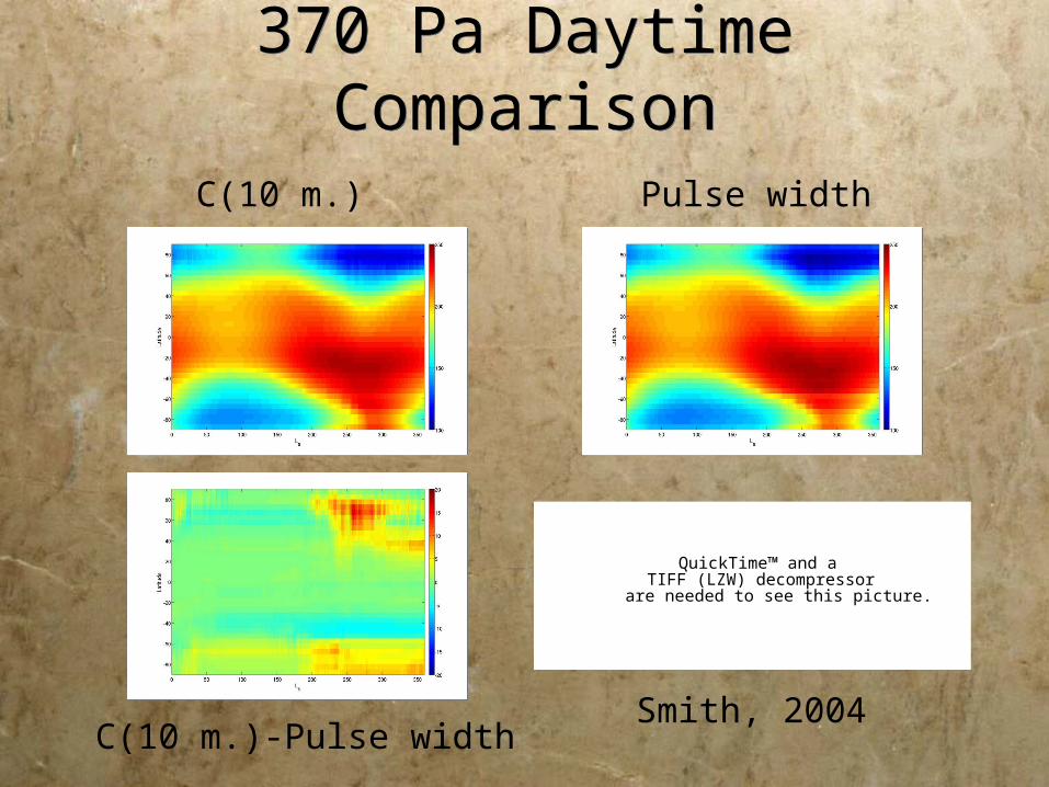
370 Pa Daytime Comparison
370 Pa Daytime Comparison
QuickTime™ and aTIFF (LZW) decompressor
are needed to see this picture.
Smith, 2004
C(10 m.) Pulse width
C(10 m.)-Pulse width
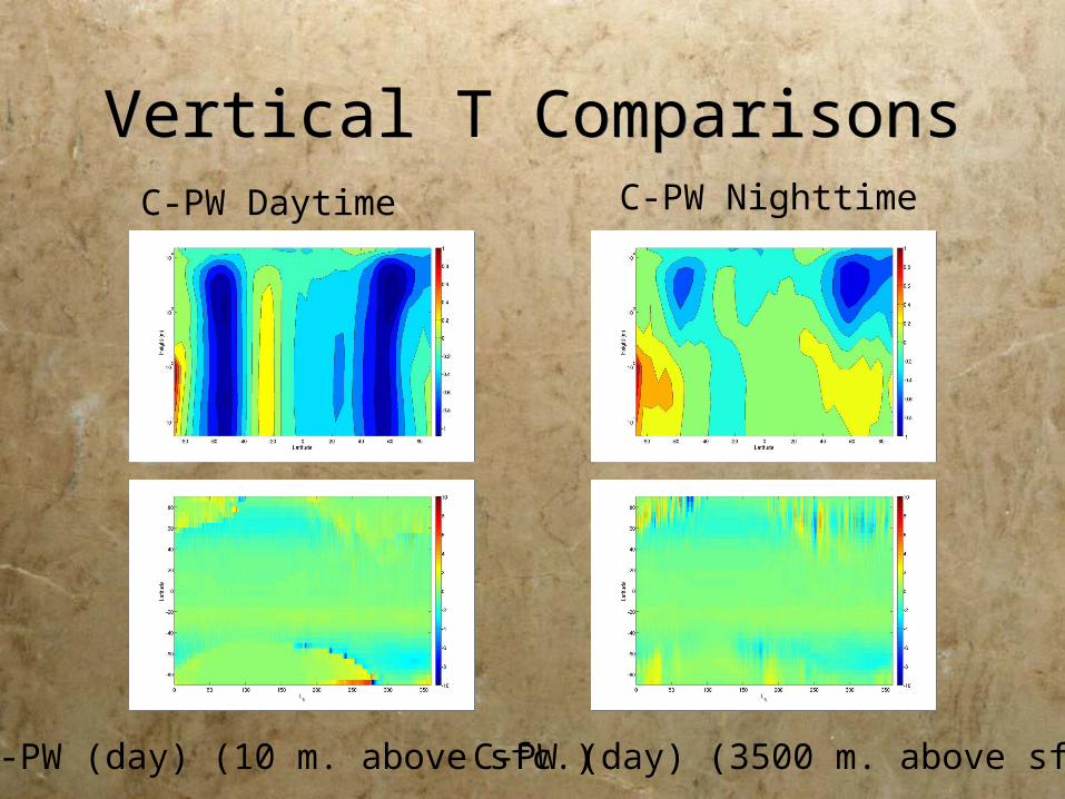
Vertical T ComparisonsVertical T ComparisonsC-PW Daytime C-PW Nighttime
C-PW (day) (10 m. above sfc.) C-PW (day) (3500 m. above sfc.)

Implications for Dust Devil Activity
Implications for Dust Devil Activity
Kurgansky (2006) proposed that dust devil size distribution strong function of |l|
Hess and Spillane (1990) proposed that Dust Devil Activity in General, a strong function of 1/|L|.
Combination Could Result in High dust devil Density in High Lats, Large DDs at mid z0 (Amazonis Planitia?) Alternate Explanations…
Whelley et al. (2006)

SummarySummary
We present two different possible aerodynamic roughness maps (both with different controversial assumptions)
Daytime summer temperatures in high latitudes very sensitive to z0 change (reduced eddy diffusion wins over convection)
Smoothness of high latitudes may explain high dust devil activity (provided tracks are a Good Metric)