martingales, nonlinearity, and chaosfinance.martinsewell.com/.../nonlinearity/... · journal of...

Journal of Economic Dynamics & Control24 (2000) 703}724

Martingales, nonlinearity, and chaos

William A. Barnett!,*, Apostolos Serletis"

!Department of Economics, Campus Box 1208, Washington University, One Brookings Drive, St. Louis,MO 63130-4810, USA

"Department of Economics, The University of Calgary, Calgary, Alberta T2N 1N4, USA

Abstract

In this article we provide a review of the literature with respect to the e$cient marketshypothesis and chaos. In doing so, we contrast the martingale behavior of asset prices tononlinear chaotic dynamics, discuss some recent techniques used in distinguishingbetween probabilistic and deterministic behavior in asset prices, and report some evid-ence. Moreover, we look at the controversies that have arisen about the available testsand results, and raise the issue of whether dynamical systems theory is practical in"nance. ( 2000 Elsevier Science B.V. All rights reserved.

JEL classixcation: C22; G14

Keywords: E$cient markets hypothesis; Chaotic dynamics

1. Introduction

Recently, the e$cient markets hypothesis and the notions connected with ithave provided the basis for a great deal of research in "nancial economics.A voluminous literature has developed supporting this hypothesis. Brie#ystated, the hypothesis claims that asset prices are rationally related to economic

*Corresponding author.E-mail address: [email protected] (W.A. Barnett)The authors would like to thank Cars Hommes and Dee Dechert for useful comments. Serletis

acknowledges "nancial support from the SSHRCC.

0165-1889/00/$ - see front matter ( 2000 Elsevier Science B.V. All rights reserved.PII: S 0 1 6 5 - 1 8 8 9 ( 9 9 ) 0 0 0 2 3 - 8

realities and always incorporate all the information available to the market. Thisimplies the absence of exploitable excess pro"t opportunities. However, despitethe widespread allegiance to the notion of market e$ciency, a number of studieshave suggested that certain asset prices are not rationally related to economicrealities. For example, Summers (1986) argues that market valuations di!ersubstantially and persistently from rational valuations and that existing evid-ence (based on common techniques) does not establish that "nancial marketsare e$cient.

Although most of the empirical tests of the e$cient markets hypothesis arebased on linear models, interest in nonlinear chaotic processes has in the recentpast experienced a tremendous rate of development. There are many reasons forthis interest, one of which being the ability of such processes to generate outputthat mimics the output of stochastic systems, thereby o!ering an alternativeexplanation for the behavior of asset prices. In fact, the possible existence ofchaos could be exploitable and even invaluable. If, for example, chaos can beshown to exist in asset prices, the implication would be that pro"table, nonlin-earity-based trading rules exist (at least in the short run and provided the actualgenerating mechanism is known). Prediction, however, over long periods is allbut impossible, due to the sensitive dependence on initial conditions property ofchaos.

In this paper, we survey the recent literature with respect to the e$cientmarkets hypothesis and chaos. In doing so, in the next two sections webrie#y discuss the e$cient markets hypothesis and some of the more recenttesting methodologies. In Section 4, we provide a description of the keyfeatures of the available tests for independence, nonlinearity, and chaos,focusing explicit attention on each test's ability to detect chaos. InSection 5, we present a discussion of the empirical evidence on macroeconomicand (mostly) "nancial data, and in Section 6, we look at the controversiesthat have arisen about the available tests and address some importantquestions regarding the power of some of these tests. The "nal sectionconcludes.

2. The martingale hypothesis

Standard asset pricing models typically imply the &martingale model', accord-ing to which tomorrow's price is expected to be the same as today's price.Symbolically, a stochastic process x

tfollows a martingale if

Et(x

t`1DX

t)"x

t, (1)

where Xtis the time t information set* assumed to include x

t. Eq. (1) says that if

xtfollows a martingale the best forecast of x

t`1that could be constructed based

on current information Xtwould just equal x

t.

704 W.A. Barnett, A. Serletis / Journal of Economic Dynamics & Control 24 (2000) 703}724

Alternatively, the martingale model implies that (xt`1

!xt) is a &fair game'

(a game which is neither in your favor nor your opponent's)1

Et[(x

t`1!x

t)DX

t]"0. (2)

Clearly, xtis a martingale if and only if (x

t`1!x

t) is a fair game. It is for this

reason that fair games are sometimes called &martingale di!erences'.2 The fairgame model (2) says that increments in value (changes in price adjusted fordividends) are unpredictable, conditional on the information set X

t. In this sense,

information Xtis fully re#ected in prices and hence useless in predicting rates of

return. The hypothesis that prices fully re#ect available information has come tobe known as the &e$cient markets hypothesis'.

In fact Fama (1970) de"ned three types of (informational) capital markete$ciency (not to be confused with allocational or Pareto-e$ciency), each ofwhich is based on a di!erent notion of exactly what type of information isunderstood to be relevant. In particular, markets are weak-form, semistrong-form, and strong-form e$cient if the information set includes past prices andreturns alone, all public information, and any information public as well asprivate, respectively. Clearly, strong-form e$ciency implies semistrong-forme$ciency, which in turn implies weak-form e$ciency, but the reverse implica-tions do not follow, since a market easily could be weak-form e$cient butnot semistrong-form e$cient or semistrong-form e$cient but not strong-forme$cient.

The martingale model given by (1) can be written equivalently as

xt`1

"xt#e

t,

where etis the martingale di!erence. When written in this form the martingale

looks identical to the &random walk model' * the forerunner of the theory ofe$cient capital markets. The martingale, however, is less restrictive than therandom walk. In particular, the martingale di!erence requires only indepen-dence of the conditional expectation of price changes from the available in-formation, as risk neutrality implies, whereas the (more restrictive) random walkmodel requires this and also independence involving the higher conditionalmoments (i.e., variance, skewness, and kurtosis) of the probability distribution ofprice changes.

1A stochastic process ztis a fair game if z

thas the property E

t(z

t`1DX

t)"0.

2The martingale process is a special case of the more general submartingale process. In particular,xtis a &submartingale' if it has the property E

t(x

t`1DX

t)5x

t. In terms of the (x

t`1!x

t) process, the

submartingale model implies that Et[(x

t`1!x

t)DX

t]50 and embodies the concept of a superfair

game. LeRoy (1989, pp. 1593}1594) also o!ers an example in which Et[(x

t`1!x

t)DX

t]40, in which

case xtwill be a &supermartingale', embodying the concept of a subfair game.

W.A. Barnett, A. Serletis / Journal of Economic Dynamics & Control 24 (2000) 703}724 705

In fact, Campbell et al. (1997) distinguish between three versions of therandom walk hypothesis* the &independently and identically distributed-re-turns' version, the &independent-returns' version, and the version of &uncor-related-returns'* see Campbell et al. (1997) for more details. The martingaledi!erence model, by not requiring probabilistic independence between success-ive price changes, is entirely consistent with the fact that price changes, althoughuncorrelated, tend not to be independent over time but to have clusters ofvolatility and tranquility (i.e., dependence in the higher conditional moments)* a phenomenon originally noted for stock market prices by Mandelbrot (1963)and Fama (1965).

3. Tests of the martingale hypothesis

The random walk and martingale hypotheses imply a unit root in the level ofthe price or logarithm of the price series* notice that a unit root is a necessarybut not su$cient condition for the random walk and martingale models to hold.Hence, these models can be tested using recent advances in the theory ofintegrated regressors. The literature on unit root testing is vast and, in whatfollows, we shall only brie#y illustrate some of the issues that have arisen in thebroader search for unit roots in "nancial asset prices.3

Nelson and Plosser (1982), using the augmented Dickey}Fuller (ADF) unitroot testing procedure (see Dickey and Fuller, 1981) test the null hypothesis of&di!erence-stationarity' against the &trend-stationarity' alternative. In particular,in the context of "nancial asset prices, one would estimate the followingregression:

*yt"a

0#a

1yt~1

#

l

+j/1

cj*y

t~j#e

t,

where y denotes the logarithm of the series. The null hypothesis of a single unitroot is rejected if a

1is negative and signi"cantly di!erent from zero. A trend

variable should not be included, since the presence of a trend in "nancial assetprices is a clear violation of market e$ciency, whether or not the asset price hasa unit root. The optimal lag length, l, can be chosen using data-dependentmethods, that have desirable statistical properties when applied to unit roottests. Based on such ADF unit root tests, Nelson and Plosser (1982) argue thatmost macroeconomic and "nancial time series have a unit root.

3 It is to be noted that unit root tests have low power against relevent alternatives. Also, asGranger (1995) points out, nonlinear modelling of nonstationary variables is a new, complicated,and largely undeveloped area. We therefore ignore this issue in this paper, keeping in mind that thisis an area for future research.


Perron (1989), however, argues that most time series [and in particular thoseused by Nelson and Plosser (1982)] are trend stationary if one allows fora one-time change in the intercept or in the slope (or both) of the trend function.The postulate is that certain &big shocks' do not represent a realization of theunderlying data generation mechanism of the series under consideration andthat the null should be tested against the trend-stationary alternative by allow-ing, under both the null and the alternative hypotheses, for the presence ofa one-time break (at a known point in time) in the intercept or in the slope (orboth) of the trend function.4 Hence, whether the unit root model is rejected ornot depends on how big shocks are treated. If they are treated like any othershock, then ADF unit root testing procedures are appropriate and the unit rootnull hypothesis cannot (in general) be rejected. If, however, they are treateddi!erently, then Perron-type procedures are appropriate and the null hypothesisof a unit root will most likely be rejected.

Finally, given that integration tests are sensitive to the class of modelsconsidered (and may be misleading because of misspeci"cation), &fractionally'integrated representations, which nest the unit-root phenomenon in a moregeneral model, have also been used* see Baillie (1996) for a survey. Fractionalintegration is a popular way to parameterize long-memory processes. If suchprocesses are estimated with the usual autoregressive-moving average model,without considering fractional orders of integration, the estimated autoregres-sive process can exhibit spuriously high persistence close to a unit root. Since"nancial asset prices might depart from their means with long memory, onecould condition the unit root tests on the alternative of a fractional integratedprocess, rather than the usual alternative of the series being stationary. In thiscase, if we fail to reject an autoregressive unit root, we know it is not a spurious"nding due to neglect of the relevant alternative of fractional integration andlong memory.

Despite the fact that the random walk and martingale hypotheses are con-tained in the null hypothesis of a unit root, unit root tests are not predictabilitytests. They are designed to reveal whether a series is di!erence stationary ortrend stationary and as such they are tests of the permanent/temporary natureof shocks. More recently, a series of papers including those by Poterba andSummers (1988), and Lo and MacKinlay (1988) have argued that the e$cientmarkets theory can be tested by comparing the relative variability of returns

4Perron's (1989) assumption that the break point is uncorrelated with the data has been criticized,on the basis that problems associated with &pre-testing' are applicable to his methodology and thatthe structural break should instead be treated as being correlated with the data. More recently,a number of studies treat the selection of the break point as the outcome of an estimation procedureand transform Perron's (1989) conditional (on structural change at a known point in time) unit roottest into an unconditional unit root test.


over di!erent horizons using the variance ratio methodology of Cochrane(1988). They have shown that asset prices are mean reverting over long invest-ment horizons* that is, a given price change tends to be reversed over the nextseveral years by a predictable change in the opposite direction. Similar resultshave been obtained by Fama and French (1988), using an alternative but closelyrelated test based on predictability of multiperiod returns. Of course, mean-reverting behavior in asset prices is consistent with transitory deviations fromequilibrium which are both large and persistent, and implies positive autocorre-lation in returns over short horizons and negative autocorrelation over longerhorizons.

Predictability of "nancial asset returns is a broad and very active researchtopic and a complete survey of the vast literature is beyond the scope of thepresent paper. We shall notice, however, that a general consensus has emergedthat asset returns are predictable. As Campbell et al. (1997, pp. 80) put it`[r]ecent econometric advances and empirical evidence seem to suggest that"nancial asset returns are predictable to some degree. Thirty years ago thiswould have been tantamount to an outright rejection of market e$ciency.However, modern "nancial economics teaches us that other, perfectly rational,factors may account for such predictability. The "ne structure of securitiesmarkets and frictions in the trading process can generate predictability. Time-varying expected returns due to changing business conditions can generatepredictability. A certain degree of predictability may be necessary to rewardinvestors for bearing certain dynamic risksa.

4. Tests of nonlinearity and chaos

Most of the empirical tests that we discussed so far are designed to detect&linear' structure in "nancial data * that is, linear predictability is the focus.However, as Campbell, et al. (1997, pp. 467) argue &2 many aspects of economicbehavior may not be linear. Experimental evidence and casual introspectionsuggest that investors' attitudes towards risk and expected return are nonlinear.The terms of many "nancial contracts such as options and other derivativesecurities are nonlinear. And the strategic interactions among market partici-pants, the process by which information is incorporated into security prices, andthe dynamics of economy-wide #uctuations are all inherently nonlinear. There-fore, a natural frontier for "nancial econometrics is the modeling of nonlinearphenomena'.

It is for such reasons that interest in deterministic nonlinear chaotic processeshas in the recent past experienced a tremendous rate of development. Besides itsobvious intellectual appeal, chaos is interesting because of its ability to generateoutput that mimics the output of stochastic systems, thereby o!ering an alterna-tive explanation for the behavior of asset prices. Clearly then, an important area


for potentially productive research is to test for chaos and (in the event that itexists) to identify the nonlinear deterministic system that generates it. In whatfollows, we turn to several univariate statistical tests for independence, non-linearity and chaos, that have been recently motivated by the mathematics ofdeterministic nonlinear dynamical systems.

4.1. The correlation dimension test

Grassberger and Procaccia (1983) suggested the &correlation dimension' testfor chaos. To brie#y discuss this test, let us start with the one-dimensional series,Mx

tNnt/1

, which can be embedded into a series of m-dimensional vectorsX

t"(x

t,x

t~1,2,x

t~m`1)@ giving the series MX

tNnt/m

. The selected value of m iscalled the &embedding dimension' and each X

tis known as an &m-history' of the

series MxtNnt/1

. This converts the series of scalars into a slightly shorter series of(m-dimensional) vectors with overlapping entries * in particular, from thesample size n, N"n!m#1 m-histories can be made. Assuming that the true,but unknown, system which generated Mx

tNnt/1

is 0 -dimensional and providedthat m520#1, then the N m-histories recreate the dynamics of the datageneration process and can be used to analyze the dynamics of the system* seeTakens (1981).

The correlation dimension test is based on the &correlation function' (or&correlation integral'), C(N,m, e), which for a given embedding dimension m isgiven by

C(N,m, e)"1

N(N!1)+

mytEsyn

H(e!DDXt!X

sDD),

where e is a su$ciently small number, H(z) is the Heavside function (which mapspositive arguments into 1 and nonpositive arguments into 0), and DD.DD denotes thedistance induced by the selected norm (the &maximum norm' being the type usedmost often). In other words, the correlation integral is the number of pairs (t, s)such that each corresponding component of X

tand X

sare near to each other,

nearness being measured in terms of distance being less than e. Intuitively,C(N,m, e) measures the probability that the distance between any twom-histories is less than e. If C(N,m, e) is large (which means close to 1) for a verysmall e, then the data is very well correlated.

The correlation dimension can be de"ned as

Dm#"lim

e?0

logC(N,m, e)log e

,

that is by the slope of the regression of logC(N,m, e) versus log e for small valuesof e, and depends on the embedding dimension, m. As a practical matter oneinvestigates the estimated value of Dm

#as m is increased. If as m increases


Dm#

continues to rise, then the system is stochastic. If, however, the data aregenerated by a deterministic process (consistent with chaotic behavior), thenDm

#reaches a "nite saturation limit beyond some relatively small m.5 The correla-

tion dimension can therefore be used to distinguish true stochastic processesfrom deterministic chaos (which may be low-dimensional or high-dimensional).

While the correlation dimension measure is therefore potentially very usefulin testing for chaos, the sampling properties of the correlation dimension are,however, unknown. As Barnett et al. (1995, pp. 306) put it `[i]f the only source ofstochasticity is [observational] noise in the data, and if that noise is slight, thenit is possible to "lter the noise out of the data and use the correlation dimensiontest deterministically. However, if the economic structure that generated thedata contains a stochastic disturbance within its equations, the correlationdimension is stochastic and its derived distribution is important in producingreliable inferencea.

Moreover, if the correlation dimension is very large as in the case of high-dimensional chaos, it will be very di$cult to estimate it without an enormousamount of data. In this regard, Ruelle (1990) argues that a chaotic series can onlybe distinguished if it has a correlation dimension well below 2 log

10N, where

N is the size of the data set, suggesting that with economic time series thecorrelation dimension can only distinguish low-dimensional chaos from high-dimensional stochastic processes* see also Grassberger and Procaccia (1983)for more details.

4.2. The BDS test

To deal with the problems of using the correlation dimension test, Brock et al.(1996) devised a new statistical test which is known as the BDS test* see alsoBrock et al. (1991). The BDS tests the null hypothesis of whiteness (independentand identically distributed observations) against an unspeci"ed alternative usinga nonparametric technique.

The BDS test is based on the Grassberger and Procaccia (1983) correlationintegral as the test statistic. In particular, under the null hypothesis of whiteness,the BDS statistic is

=(N,m, e)"JNC(N,m, e)!C(N, 1, e)m

p( (N,m, e)

5Since the correlation dimension can be used to characterize both chaos and stochastic dynamics(i.e., the correlation dimension is a "nite number in the case of chaos and equal to in"nity in the caseof an independent and identically distributed stochastic process), one often "nds in the literatureexpressions like &deterministic chaos' (meaning simply chaos) and &stochastic chaos' (meaningstandard stochastic dynamics). This terminology, however, is confusing in contexts other than thatof the correlation dimension analysis and we shall not use it here.


where p( (N, m, e) is an estimate of the asymptotic standard deviation ofC(N,m, e)!C(N, 1, e)m* the formula for p( (N,m, e) can be found in Brock et al.(1996). The BDS statistic is asymptotically standard normal under the whitenessnull hypothesis * see Brock et al. (1996) for details.

The intuition behind the BDS statistic is as follows. C(N,m, e) is an estimate ofthe probability that the distance between any two m-histories, X

tand X

sof the

series MxtN is less than e. If Mx

tN were independent then for tOs the probability of

this joint event equals the product of the individual probabilities. Moreover, ifMx

tN were also identically distributed then all of the m probabilities under the

product sign are the same. The BDS statistic therefore tests the null hypothesisthat C(N,m, e)"C(N, 1, e)m * the null hypothesis of whiteness.6

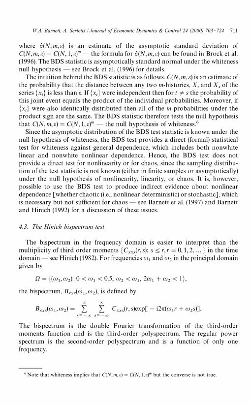
Since the asymptotic distribution of the BDS test statistic is known under thenull hypothesis of whiteness, the BDS test provides a direct (formal) statisticaltest for whiteness against general dependence, which includes both nonwhitelinear and nonwhite nonlinear dependence. Hence, the BDS test does notprovide a direct test for nonlinearity or for chaos, since the sampling distribu-tion of the test statistic is not known (either in "nite samples or asymptotically)under the null hypothesis of nonlinearity, linearity, or chaos. It is, however,possible to use the BDS test to produce indirect evidence about nonlineardependence [whether chaotic (i.e., nonlinear deterministic) or stochastic], whichis necessary but not su$cient for chaos* see Barnett et al. (1997) and Barnettand Hinich (1992) for a discussion of these issues.

4.3. The Hinich bispectrum test

The bispectrum in the frequency domain is easier to interpret than themultiplicity of third order moments MC

xxx(r, s): s4r, r"0, 1, 2,2N in the time

domain* see Hinich (1982). For frequencies u1

and u2in the principal domain

given by

X"M(u1,u

2): 0(u

1(0.5, u

2(u

1, 2u

1#u

2(1N,

the bispectrum, Bxxx

(u1,u

2), is de"ned by

Bxxx

(u1,u

2)"

=+

r/~=

=+

s/~=

Cxxx

(r, s)exp[!i2n(u1r#u

2s)].

The bispectrum is the double Fourier transformation of the third-ordermoments function and is the third-order polyspectrum. The regular powerspectrum is the second-order polyspectrum and is a function of only onefrequency.

6Note that whiteness implies that C(N,m, e)"C(N, 1, e)m but the converse is not true.


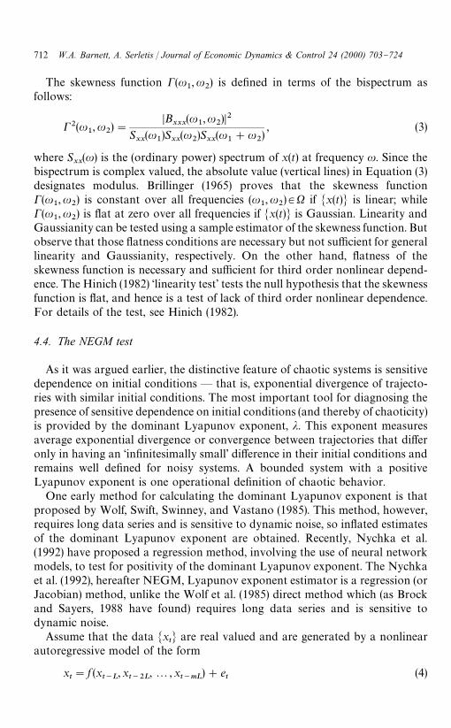
The skewness function C(u1, u

2) is de"ned in terms of the bispectrum as

follows:

C2(u1, u

2)"

DBxxx

(u1,u

2)D2

Sxx

(u1)S

xx(u

2)S

xx(u

1#u

2), (3)

where Sxx

(u) is the (ordinary power) spectrum of x(t) at frequency u. Since thebispectrum is complex valued, the absolute value (vertical lines) in Equation (3)designates modulus. Brillinger (1965) proves that the skewness functionC(u

1, u

2) is constant over all frequencies (u

1, u

2)3X if Mx(t)N is linear; while

C(u1, u

2) is #at at zero over all frequencies if Mx(t)N is Gaussian. Linearity and

Gaussianity can be tested using a sample estimator of the skewness function. Butobserve that those #atness conditions are necessary but not su$cient for generallinearity and Gaussianity, respectively. On the other hand, #atness of theskewness function is necessary and su$cient for third order nonlinear depend-ence. The Hinich (1982) &linearity test' tests the null hypothesis that the skewnessfunction is #at, and hence is a test of lack of third order nonlinear dependence.For details of the test, see Hinich (1982).

4.4. The NEGM test

As it was argued earlier, the distinctive feature of chaotic systems is sensitivedependence on initial conditions * that is, exponential divergence of trajecto-ries with similar initial conditions. The most important tool for diagnosing thepresence of sensitive dependence on initial conditions (and thereby of chaoticity)is provided by the dominant Lyapunov exponent, j. This exponent measuresaverage exponential divergence or convergence between trajectories that di!eronly in having an &in"nitesimally small' di!erence in their initial conditions andremains well de"ned for noisy systems. A bounded system with a positiveLyapunov exponent is one operational de"nition of chaotic behavior.

One early method for calculating the dominant Lyapunov exponent is thatproposed by Wolf, Swift, Swinney, and Vastano (1985). This method, however,requires long data series and is sensitive to dynamic noise, so in#ated estimatesof the dominant Lyapunov exponent are obtained. Recently, Nychka et al.(1992) have proposed a regression method, involving the use of neural networkmodels, to test for positivity of the dominant Lyapunov exponent. The Nychkaet al. (1992), hereafter NEGM, Lyapunov exponent estimator is a regression (orJacobian) method, unlike the Wolf et al. (1985) direct method which (as Brockand Sayers, 1988 have found) requires long data series and is sensitive todynamic noise.

Assume that the data MxtN are real valued and are generated by a nonlinear

autoregressive model of the form

xt"f (x

t~L,x

t~2L,2,x

t~mL)#e

t(4)


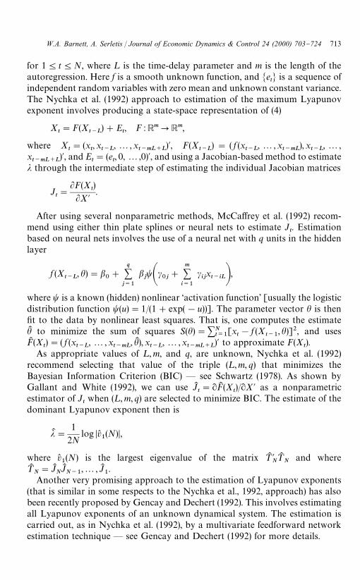
for 14t4N, where ¸ is the time-delay parameter and m is the length of theautoregression. Here f is a smooth unknown function, and Me

tN is a sequence of

independent random variables with zero mean and unknown constant variance.The Nychka et al. (1992) approach to estimation of the maximum Lyapunovexponent involves producing a state-space representation of (4)

Xt"F(X

t~L)#E

t, F : RmPRm,

where Xt"(x

t, x

t~L,2,x

t~mL`L)@, F(X

t~L)" ( f (x

t~L,2,x

t~mL),x

t~L,2,

xt~mL`L

)@, and Et"(e

t, 0,2,0)@, and using a Jacobian-based method to estimate

j through the intermediate step of estimating the individual Jacobian matrices

Jt"

LF(Xt)

LX@.

After using several nonparametric methods, McCa!rey et al. (1992) recom-mend using either thin plate splines or neural nets to estimate J

t. Estimation

based on neural nets involves the use of a neural net with q units in the hiddenlayer

f (Xt~L

, h)"b0#

q+j/1

bjtAc0j#

m+i/1

cijxt~iLB,

where t is a known (hidden) nonlinear &activation function' [usually the logisticdistribution function t(u)"1/(1#exp(!u))]. The parameter vector h is then"t to the data by nonlinear least squares. That is, one computes the estimatehK to minimize the sum of squares S(h)"+N

t/1[x

t!f (X

t~1, h)]2, and uses

FK (Xt)"( f (x

t~L,2,x

t~mL, hK ),x

t~L,2,x

t~mL`L)@ to approximate F(X

t).

As appropriate values of ¸, m, and q, are unknown, Nychka et al. (1992)recommend selecting that value of the triple (¸,m, q) that minimizes theBayesian Information Criterion (BIC) * see Schwartz (1978). As shown byGallant and White (1992), we can use JK

t"RFK (X

t)/RX@ as a nonparametric

estimator of Jtwhen (¸, m, q) are selected to minimize BIC. The estimate of the

dominant Lyapunov exponent then is

jK "1

2Nlog Dv(

1(N)D,

where v(1(N) is the largest eigenvalue of the matrix ¹K @

N¹K

Nand where

¹KN"JK

NJKN~1

,2, JK1.

Another very promising approach to the estimation of Lyapunov exponents(that is similar in some respects to the Nychka et al., 1992, approach) has alsobeen recently proposed by Gencay and Dechert (1992). This involves estimatingall Lyapunov exponents of an unknown dynamical system. The estimation iscarried out, as in Nychka et al. (1992), by a multivariate feedforward networkestimation technique * see Gencay and Dechert (1992) for more details.


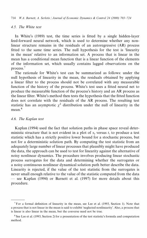
4.5. The White test

In White's (1989) test, the time series is "tted by a single hidden-layerfeed-forward neural network, which is used to determine whether any non-linear structure remains in the residuals of an autoregressive (AR) process"tted to the same time series. The null hypothesis for the test is &linearityin the mean' relative to an information set. A process that is linear in themean has a conditional mean function that is a linear function of the elementsof the information set, which usually contains lagged observations on theprocess.7

The rationale for White's test can be summarized as follows: under thenull hypothesis of linearity in the mean, the residuals obtained by applyinga linear "lter to the process should not be correlated with any measurablefunction of the history of the process. White's test uses a "tted neural net toproduce the measurable function of the process's history and an AR process asthe linear "lter. White's method then tests the hypothesis that the "tted functiondoes not correlate with the residuals of the AR process. The resulting teststatistic has an asymptotic s2 distribution under the null of linearity in themean.8

4.6. The Kaplan test

Kaplan (1994) used the fact that solution paths in phase space reveal deter-ministic structure that is not evident in a plot of x

tversus t, to produce a test

statistic which has a strictly positive lower bound for a stochastic process, butnot for a deterministic solution path. By computing the test statistic from anadequately large number of linear processes that plausibly might have producedthe data, the approach can be used to test for linearity against the alternative ofnoisy nonlinear dynamics. The procedure involves producing linear stochasticprocess surrogates for the data and determining whether the surrogates ora noisy continuous nonlinear dynamical solution path better describe the data.Linearity is rejected, if the value of the test statistic from the surrogates isnever small enough relative to the value of the statistic computed from the data* see Kaplan (1994) or Barnett et al. (1997) for more details about thisprocedure.

7For a formal de"nition of linearity in the mean, see Lee et al. (1993, Section 1). Note thata process that is not linear in the mean is said to exhibit &neglected nonlinearity'. Also, a process thatis linear is also linear in the mean, but the converse need not be true.

8See Lee et al. (1993, Section 2) for a presentation of the test statistic's formula and computationmethod.


5. Evidence on nonlinearity and chaos

A number of researchers have recently focused on testing for nonlinearity ingeneral and chaos in particular in macroeconomic time series. There are manyreasons for this interest. Chaos, for example, represents a radical change ofperspective on business cycles. Business cycles receive an endogenous explanationand are traced back to the strong nonlinear deterministic structure that canpervade the economic system. This is di!erent from the (currently dominant)exogenous approach to economic #uctuations, based on the assumption thateconomic equilibria are determinate and intrinsically stable, so that in the absenceof continuing exogenous shocks the economy tends towards a steady state, butbecause of stochastic shocks a stationary pattern of #uctuations is observed.9

There is a broad consensus of support for the proposition that the (macroeco-nomic) data generating processes are characterized by a pattern of nonlineardependence, but there is no consensus at all on whether there is chaos inmacroeconomic time series. For example, Brock and Sayers (1988), Frank andStengos (1988), and Frank et al. (1988) "nd no evidence of chaos in U.S.,Canadian, and international, respectively, macroeconomic time series. On theother hand, Barnett and Chen (1988), claimed successful detection of chaos inthe (demand-side) U.S. Divisia monetary aggregates. Their conclusion wasfurther con"rmed by DeCoster and Mitchell (1991,1994). This published claimof successful detection of chaos has generated considerable controversy, as inRamsey et al. (1990) and Ramsey and Rothman (1994), who raised questionsregarding virtually all published tests of chaos. Further results relevant to thiscontroversy have recently been provided by Serletis (1995).

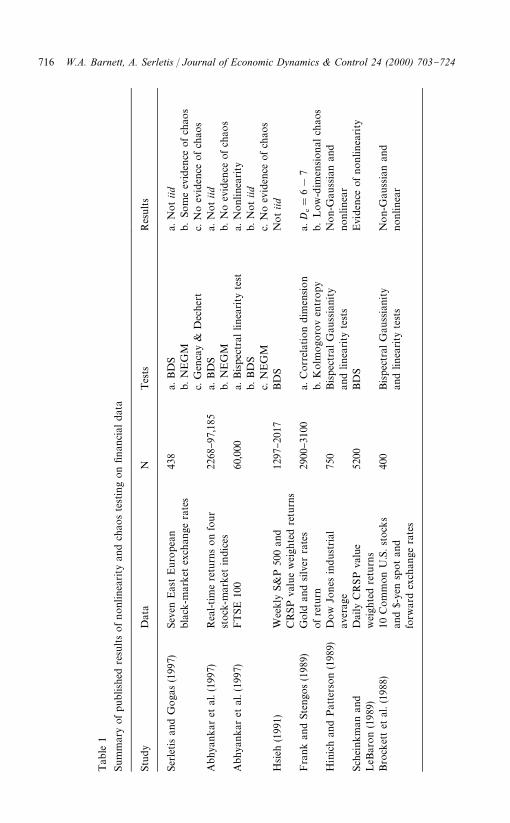
Although the analysis of macroeconomic time series has not yet led toparticularly encouraging results (mainly due to the small samples and high noiselevels for most macroeconomic series), as can be seen from Table 1, there is alsoa substantial literature testing for nonlinear dynamics on "nancial data.10 Thisliterature has led to results which are as a whole more interesting and morereliable than those of macroeconomic series, probably due to the much largernumber of data available and their superior quality (measurement in most casesis more precise, at least when we do not have to make recourse to broadaggregation). As regards the main conclusions of this literature, there is clearevidence of nonlinear dependence and some evidence of chaos.

9Chaos could also help unify di!erent approaches to structural macroeconomics. As Grandmont(1985) has shown, for di!erent parameter values even the most classical of economic models canproduce stable solutions (characterizing classical economics) or more complex solutions, such ascycles or even chaos (characterizing much of Keynesian economics)

10For other unpublished work on testing nonlinearity and chaos on "nancial data, seeAbhyankar et al. (1997, Table 1).


Tab

le1

Sum

mar

yof

publis

hed

resu

lts

ofnon

linea

rity

and

chao

ste

stin

gon"nan

cial

dat

a

Stu

dyD

ata

NTes

tsR

esults

Ser

letis

and

Goga

s(1

997)

Sev

enEas

tEuro

pean

438

a.B

DS

a.N

ot

iid

bla

ck-m

arket

exch

ange

rate

sb.N

EG

Mb.

Som

eev

iden

ceofch

aos

c.G

enca

y&

Dec

hert

c.N

oev

iden

ceofch

aos

Abhy

ankar

etal

.(19

97)

Rea

l-tim

ere

turn

son

four

stock

-mar

ket

indi

ces

2268}97

,185

a.B

DS

a.N

ot

iid

b.N

EG

Mb.

No

evid

ence

ofch

aos

Abhy

ankar

etal

.(19

97)

FT

SE

100

60,0

00a.

Bispec

tral

linea

rity

test

a.N

onl

inea

rity

b.BD

Sb.N

ot

iid

c.N

EG

Mc.

No

evid

ence

ofch

aos

Hsieh

(199

1)W

eekl

yS&

P50

0an

d12

97}20

17BD

SN

ot

iid

CR

SPva

lue

wei

ghte

dre

turn

sFra

nkan

dSt

engo

s(1

989)

Gold

and

silv

erra

tes

2900}31

00a.

Cor

rela

tion

dim

ension

a.D

#"6!

7ofre

turn

b.K

olm

ogo

rov

entr

opy

b.

Low

-dim

ensional

chao

sH

inic

han

dP

atte

rson

(198

9)D

ow

Jones

indus

tria

l75

0Bispec

tral

Gau

ssia

nity

Non-

Gau

ssia

nan

dav

erag

ean

dlin

earity

test

snonlin

ear

Sche

inkm

anan

dLeB

aron

(198

9)D

aily

CR

SP

valu

e52

00BD

SEvi

denc

eof

nonlin

earity

wei

ghte

dre

turn

sBro

cket

tet

al.(1

988)

10C

om

mon

U.S

.st

ocks

400

Bispec

tral

Gau

ssia

nity

Non-

Gau

ssia

nan

dan

d$-

yen

spot

and

and

linea

rity

test

snonlin

ear

forw

ard

exch

ange

rate

s


For example, Scheinkman and LeBaron (1989) studied United States weeklyreturns on the Center for Research in Security Prices (CRSP) value-weightedindex, employing the BDS statistic, and found rather strong evidence of non-linearity and some evidence of chaos.11 Some very similar results have beenobtained by Frank and Stengos (1989), investigating daily prices (from themid-1970s to the mid-1980s) for gold and silver, using the correlation dimensionand the Kolmogorov entropy. Their estimate of the correlation dimension wasbetween 6 and 7 for the original series and much greater and non-converging forthe reshu%ed data.

More recently, Serletis and Gogas (1997) test for chaos in seven East Euro-pean black market exchange rates, using the Koedijk and Kool (1992) monthlydata (from January 1955 through May 1990). In doing so, they use threeinference methods, the BDS test, the NEGM test, as well as the Lyapunovexponent estimator of Gencay and Dechert (1992). They "nd some consistencyin inference across methods, and conclude, based on the NEGM test, that thereis evidence consistent with a chaotic nonlinear generation process in two out ofthe seven series* the Russian ruble and East German mark. Altogether, theseand similar results seem to suggest that "nancial series provide a more promis-ing "eld of research for the methods in question.

A notable feature of the literature just summarized is that most researchers, inorder to "nd su$cient observations to implement the tests, use data periodsmeasured in years. The longer the data period, however, the less plausible is theassumption that the underlying data generation process has remained station-ary, thereby making the results di$cult to interpret. In fact, di!erent conclusionshave been reached by researchers using high-frequency data over short periods.For example, Abhyankar et al. (1995) examine the behavior of the U.K. Finan-cial Times Stock Exchange 100 (FTSE 100) index, over the "rst six months of1993 (using 1-, 5-, 15-, 30-, and 60-min returns). Using the Hinich (1982)bispectral linearity test, the BDS test, and the NEGM test, they "nd evidence ofnonlinearity, but no evidence of chaos.

More recently, Abhyankar et al. (1997) test for nonlinear dependence andchaos in real-time returns on the world's four most important stock-marketindices * the FTSE 100, the Standard & Poor 500 (S&P 500) index, the

11 In order to verify the presence of a nonlinear structure in the data, they also suggestedemploying the so-called &shu%ing diagnostic'. This procedure involves studying the residualsobtained by adapting an autoregressive model to a series and then reshu%ing these residuals. If theresiduals are totally random (i.e., if the series under scrutiny is not characterized by chaos), thedimension of the residuals and that of the shu%ed residuals should be approximately equal. Onthe contrary, if the residuals are chaotic and have some structure, then the reshu%ing must reduceor eliminate the structure and consequently increase the correlation dimension. The correlationdimension of their reshu%ed residuals always appeared to be much greater than that of the originalresiduals, which was interpreted as being consistent with chaos.


Deutscher Aktienindex (DAX), and the Nikkei 225 Stock Average. Using theBDS and the NEGM tests, and 15-s, 1-min and 5-min returns (from September1 to November 30, 1991), they reject the hypothesis of independence in favor ofa nonlinear structure for all data series, but "nd no evidence of low-dimensionalchaotic processes.

Of course, there is other work, using high-frequency data over short periods,that "nds order in the apparent chaos of "nancial markets. For example,Ghashghaie et al. (1996) analyze all worldwide 1,472,241 bid-ask quotes on U.S.dollar}German mark exchange rates between October 1, 1992 and September30, 1993. They apply physical principles and provide a mathematical explana-tion of how one trading pattern led into and then in#uenced another. As theauthors conclude, `2 we have reason to believe that the qualitative picture ofturbulence that has developed during the past 70 yrs will help our understandingof the apparently remote "eld of "nancial marketsa.

6. Controversies

Clearly, there is little agreement about the existence of chaos or even ofnonlinearity in (economic and) "nancial data, and some economists continue toinsist that linearity remains a good assumption for such data, despite the factthat theory provides very little support for that assumption. It should be noted,however, that the available tests search for evidence of nonlinearity or chaos indata without restricting the boundary of the system that could have producedthat nonlinearity or chaos. Hence these tests should reject linearity, even if thestructure of the economy is linear, but the economy is subject to shocks froma surrounding nonlinear or chaotic physical environment, as through nonlinearclimatological or weather dynamics. Under such circumstances, linearity wouldseem an unlikely inference.12

Since the available tests are not structural and hence have no ability toidentify the source of detected chaos, the alternative hypothesis of the availabletests is that no natural deterministic explanation exists for the observed eco-nomic #uctuations anywhere in the universe. In other words, the alternativehypothesis is that economic #uctuations are produced by supernatural shocksor by inherent randomness in the sense of quantum physics. Considering theimplausibility of the alternative hypothesis, one would think that "ndings ofchaos in such nonparametric tests would produce little controversy, while anyclaims to the contrary would be subjected to careful examination. Yet, in fact theopposite seems to be the case.

12 In other words, not only is there no reason in economic theory to expect linearity within thestructure of the economy, but there is even less reason to expect to "nd linearity in nature, whichproduces shocks to the system.


We argued earlier that the controversies might stem from the high noise levelthat exists in most aggregated economic time series and the relatively lowsample sizes that are available with economic data. However, it also appearsthat the controversies are produced by the nature of the tests themselves, ratherthan by the nature of the hypothesis, since linearity is a very strong nullhypothesis, and hence should be easy to reject with any test and any economicor "nancial time series on which an adequate sample size is available. Inparticular, there may be very little robustness of such tests across variations insample size, test method, and data aggregation method * see Barnett et al.(1995) on this issue.

It is also possible that none of the tests for chaos and nonlinear dynamics thatwe have discussed completely dominates the others, since some tests may havehigher power against certain alternatives than other tests, without any of thetests necessarily having higher power against all alternatives. If this is the case,each of the tests may have its own comparative advantages, and there may evenbe a gain from using more than one of the tests in a sequence designed to narrowdown the alternatives.

To explore this possibility, Barnett with the assistance of Jensen designed andran a single blind controlled experiment, in which they produced simulated datafrom various processes having linear, nonlinear chaotic, or nonlinear noncha-otic signal. They transmitted each simulated data set by email to experts inrunning each of the statistical tests that were entered into the competition. Theemailed data included no identi"cation of the generating process, so thoseindividuals who ran the tests had no way of knowing the nature of the datagenerating process, other than the sample size, and there were two sample sizes:a &small sample' size of 380 and a &large sample' size of 2000 observations.

In fact "ve generating models were used to produce samples of the small andlarge size. The models were a fully deterministic, chaotic Feigenbaum recursion(Model I), a generalized autoregressive conditional heteroskedasticity(GARCH) process (Model II), a nonlinear moving average process (Model III),an autoregressive conditional heteroskedasticity (ARCH) process (Model IV),and an autoregressive moving average (ARMA) process (Model V). Details ofthe parameter settings and noise generation method can be found in Barnettet al. (1996). The tests entered into this competition were Hinich's bispectrumtest, the BDS test, White's test, Kaplan's test, and the NEGM test of chaos.

The results of the competition are available in Barnett et al. (1997) and aresummarized in Table 2. They provide the most systematic available comparisonof tests of nonlinearity and indeed do suggest di!ering powers of each testagainst certain alternative hypotheses. In comparing the results of the tests,however, one factor seemed to be especially important: subtle di!erences existedin the de"nition of the null hypothesis, with some of the tests being tests of thenull of linearity, de"ned in three di!erent manners in the derivation of the test'sproperties, and one test being a test of the null of chaos. Hence there were four


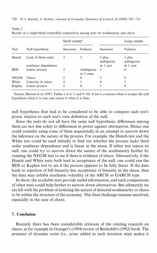
Table 2Results of a single-blind controlled competition among tests for nonlinearity and chaos

Small sample! Large sample

Test Null hypothesis Successes Failures Successes Failures

Hinich Lack of third-order 3 2 3 plusambiguous

1 plusambiguous

nonlinear dependence in 1 case in 1 caseBDS Linear process 2 Ambiguous 5 0

in 3 casesNEGM Chaos 5 0 5 0White Linearity in mean 4 1 4 1Kaplan Linear process 5 0 5 0

!Source: Barnett et al. (1997, Tables 1}4, 6}7, and 9}10). A test is a success when it accepts the nullhypothesis when it is true and rejects it when it is false.

null hypotheses that had to be considered to be able to compare each test'spower relative to each test's own de"nition of the null.

Since the tests do not all have the same null hypothesis, di!erences amongthem are not due solely to di!erences in power against alternatives. Hence onecould consider using some of them sequentially in an attempt to narrow downthe inference on the nature of the process. For example, the Hinich test and theWhite test could be used initially to "nd out whether the process lacks thirdorder nonlinear dependence and is linear in the mean. If either test rejects itsnull, one could try to narrow down the nature of the nonlinearity further byrunning the NEGM test to see if there is evidence of chaos. Alternatively, if theHinich and White tests both lead to acceptance of the null, one could run theBDS or Kaplan test to see if the process appears to be fully linear. If the dataleads to rejection of full linearity but acceptance of linearity in the mean, thenthe data may exhibit stochastic volatility of the ARCH or GARCH type.

In short, the available tests provide useful information, and such comparisonsof other tests could help further to narrow down alternatives. But ultimately weare left with the problem of isolating the nature of detected nonlinearity or chaosto be within the structure of the economy. This "nal challenge remains unsolved,especially in the case of chaos.

7. Conclusion

Recently there has been considerable criticism of the existing research onchaos, as for example in Granger's (1994) review of Benhabib's (1992) book. Thepresence of dynamic noise (i.e., noise added in each iteration step) makes it


di$cult and perhaps impossible to distinguish between (noisy) high-dimensionalchaos and pure randomness. The estimates of the fractal dimension, the correla-tion integral, and Lyapunov exponents of an underlying unknown dynamicalsystem are sensitive to dynamic noise, and the problem grows as the dimensionof the chaos increases. The question of the &impossibility' of distinguishingbetween high-dimensional chaos and randomness has recently attracted someattention, as for example in Radunskaya (1994), Bickel and BuK hlmann (1996),and Takens (1997). Analogously, Bickel and BuK hlmann (1996) argue that distin-guishing between linearity and nonlinearity of a stochastic process may becomeimpossible as the order of the linear "lter increases. In a time series framework, itis prudent to limit such tests to the use of low-order linear "lters as approxima-tions to nonlinear processes when testing for general nonlinearity, and tests forlow-dimensional chaos, when chaotic nonlinearity is of interest * see alsoBarnett et al. (1997, footnote 11).

However, in the "eld of economics, it is especially unwise to take a strongopinion (either pro or con) in that area of research. Contrary to popular opinionwithin the profession, there have been no published tests of chaos &within thestructure of the economic system', and there is very little chance that any suchtests will be available in this "eld for a very long time. Such tests are simplybeyond the state of the art. Existing tests cannot tell whether the source ofdetected chaos comes from within the structure of the economy, or from chaoticexternal shocks, as from the weather. Thus, we do not have the slightest idea ofwhether or not asset prices exhibit chaotic nonlinear dynamics produced fromthe nonlinear structure of the economy (and hence we are not justi"ed inexcluding the possibility). Until the di$cult problems of testing for chaos &withinthe structure of the economic system' are solved, the best that we can do is to testfor chaos in economic time series data, without being able to isolate its source.But even that objective has proven to be di$cult. While there have been manypublished tests for chaotic nonlinear dynamics, little agreement exists amongeconomists about the correct conclusions.

References

Abhyankar, A.H., Copeland, L.S., Wong, W., 1995. Nonlinear dynamics in real-time equity marketindices: evidence from the UK. Economic Journal 105 (431), 864}880.

Abhyankar, A.H., Copeland, L.S., Wong, W., 1997. Uncovering nonlinear structure in real-timestock-market indexes: the S&P 500, the DAX, the Nikkei 225, and the FTSE-100. Journal ofBusiness and Economic Statistics 15, 1}14.

Baillie, R.T., 1996. Long memory processes and fractional integration in econometrics. Journal ofEconometrics 73, 5}59.

Barnett, W.A., Chen, P., 1988. The aggregation-theoretic monetary aggregates are chaotic and havestrange attractors: an econometric application of mathematical chaos. In: Barnett, W.A., Berndt,E.R., White, H. (Eds.), Dynamic Econometric Modeling. Cambridge University Press,Cambridge, UK.


Barnett, W.A., Gallant, A.R., Hinich, M.J., Jungeilges, J., Kaplan, D., Jensen, M.J., 1995. Robustnessof nonlinearity and chaos tests to measurement error, inference method, and sample size. Journalof Economic Behavior and Organization 27, 301}320.

Barnett, W.A., Gallant, A.R., Hinich, M.J., Jungeilges, J., Kaplan, D., Jensen, M.J., 1996. Anexperimental design to compare tests of nonlinearity and chaos. In: Barnett, W.A., Kirman, A.,Salmon, M. (Eds.), Nonlinear Dynamics in Economics. Cambridge University Press, Cambridge,UK.

Barnett, W.A., Gallant, A.R., Hinich, M.J., Jungeilges, J., Kaplan, D., Jensen, M.J., 1997. A single-blind controlled competition among tests for nonlinearity and chaos. Journal of Econometrics82, 157}192.

Barnett, W.A., Hinich, M.J., 1992. Empirical chaotic dynamics in economics. Annals of OperationsResearch 37, 1}15.

Benhabib, J., 1992. Cycles and Chaos in Economic Equilibrium. Princeton University Press,Princeton, NJ.

Bickel, P.J., BuK hlmann, P., 1996. What is a linear process? Proceedings of the National Academy ofScience, USA, Statistics Section 93, pp. 12, 128}12,131.

Brillinger, D.R., 1965. An introduction to the polyspectrum. Annals of Mathematical Statistics 36,1351}1374.

Brock, W.A., Dechert, W.D., LeBaron, B., Scheinkman, J.A., 1996. A test for independence based onthe correlation dimension. Econometric Reviews 15, 197}235.

Brock, W.A., Hsieh, D.A., LeBaron, B., 1991. Nonlinear Dynamics, Chaos, and Instability: Statist-ical Theory and Economic Evidence. MIT Press, Cambridge, MA.

Brock, W.A., Sayers, C., 1988. Is the business cycle characterized by deterministic chaos? Journal ofMonetary Economics 22, 71}90.

Brockett, P.L., Hinich, M.J., Patterson, D., 1988. Bispectral-based tests for the detection of gaussian-ity and nonlinearity in time series. Journal of the American Statistical Association 83, 657}664.

Campbell, J.Y., Lo, A.W., MacKinlay, A.C., 1997. The Econometrics of Financial Markets.Princeton University Press, Princeton, NJ.

Cochrane, J.H., 1988. How big is the random walk in GNP? Journal of Political Economy 96,893}920.

DeCoster, G.P., Mitchell, D.W., 1991. Nonlinear monetary dynamics. Journal of Business andEconomic Statistics 9, 455}462.

DeCoster, G.P., Mitchell, D.W., 1994. Reply. Journal of Business and Economic Statistics 12,136}137.

Dickey, D.A., Fuller, W.A., 1981. Likelihood ratio tests for autoregressive time series with a unitroot. Econometrica 49, 1057}1072.

Fama, E.F., 1965. The behavior of stock market prices. Journal of Business 38, 34}105.Fama, E.F., 1970. E$cient capital markets: a review of theory and empirical work. Journal of

Finance 25, 383}417.Fama, E.F., French, K.R., 1988. Permanent and temporary components of stock prices. Journal of

Political Economy 96, 246}273.Frank, M., Gencay, R., Stengos, T., 1988. International chaos. European Economic Review 32,

569}1584.Frank, M., Stengos, T., 1988. Some evidence concerning macroeconomic chaos. Journal of

Monetary Economics 22, 423}438.Frank, M., Stengos, T., 1989. Measuring the strangeness of gold and silver rates of return. Review of

Economic Studies 56, 553}567.Gallant, R., White, H., 1992. On learning the derivatives of an unknown mapping with multilayer

feedforward networks. Neural Networks 5, 129}138.Gencay, R., Dechert, W.D., 1992. An algorithm for the n-Lyapunov exponents of an n-dimensional

unknown dynamical system. Physica D 59, 142}157.


Ghashghaie, S., Breymann, W., Peinke, J., Talkner, P., Dodge, Y., 1996. Turbulent cascades inforeign exchange markets. Nature 381, 767}770.

Grandmont, J.-M., 1985. On endogenous competitive business cycles. Econometrica 53, 995}1045.Granger, C.W.J., 1994. Is chaotic economic theory relevant for economics? A review article of: Jess

Benhabib: cycles and chaos in economic equilibrium. Journal of International and ComparativeEconomics 3, 139}145.

Granger, C.W.J., 1995. Modelling nonlinear relationships between extended-memory variables.Econometrica 63, 265}279.

Grassberger, P., Procaccia, I., 1983. Characterization of strange attractors. Physical Review Letters50, 346}349.

Hinich, M.J., 1982. Testing for gaussianity and linearity of a stationary time series. Journal of TimeSeries Analysis 3, 169}176.

Hinich, M.J., Patterson, D., 1989. Evidence of nonlinearity in the trade-by-trade stock market returngenerating process. In: Barnett, W.A., Geweke, J., Shell, K. (Eds.), Economic Complexity: Chaos,Bubbles, and Nonlinearity. Cambridge University Press, Cambridge, UK.

Hsieh, D.A., 1991. Chaos and nonlinear dynamics: applications to "nancial markets. Journal ofFinance 46, 1839}1877.

Kaplan, D.T., 1994. Exceptional events as evidence for determinism. Physica D 73, 38}48.Koedijk, K.G., Kool, C.J.M., 1992. Tail estimates of east european exchange rates. Journal of

Business and Economic Statistics 10, 83}96.Lee, T.-H., White, H., Granger, C.W.J., 1993. Testing for neglected nonlinearities in time series

models. Journal of Econometrics 56, 269}290.LeRoy, S.F., 1989. E$cient capital markets and martingales. Journal of Economic Literature 27,

1583}1621.Lo, A.W., MacKinlay, A.C., 1988. Stock market prices do not follow random walks: evidence from

a simple speci"cation test. Review of Financial Studies 1, 41}66.Mandelbrot, B.B., 1963. The variation of certain speculative stock prices. Journal of Business 36,

394}419.McCa!rey, D., Ellner, S., Gallant, R., Nychka, D., 1992. Estimating the Lyapunov exponent of

a chaotic system with nonparametric regression. Journal of the American Statistical Association87, 682}695.

Nelson, C.R., Plosser, C.I., 1982. Trends and random walks in macroeconomic time series. Journal ofMonetary Economics 10, 139}162.

Nychka, D., Ellner, S., Gallant, R., McCa!rey, D., 1992. Finding chaos in noisy systems. Journal ofthe Royal Statistical Society B 54, 399}426.

Perron, P., 1989. The great crash, the oil price shock, and the unit root hypothesis. Econometrica 57,1361}1401.

Poterba, J.M., Summers, L.H., 1988. Mean reversion in stock prices: evidence and implications.Journal of Financial Economics 22, 27}59.

Radunskaya, A., 1994. Comparing random and deterministic series. Economic Theory 4,765}776.

Ramsey, J.B., Rothman, P., 1994. Comment on &Nonlinear monetary dynamics' by DeCoster andMitchell. Journal of Business and Economic Statistics 12, 135}136.

Ramsey, J.B., Sayers, C.L., Rothman, P., 1990. The statistical properties of dimension calculationsusing small data sets: some economic applications. International Economic Review 31,991}1020.

Ruelle, D., 1990. Deterministic chaos: the science and the "ction. Proceedings of the Royal Society ofLondon A 427(1873), 241}248.

Scheinkman, J.A., LeBaron, B., 1989. Nonlinear dynamics and stock returns. Journal of Business 62,311}337.

Schwartz, G., 1978. Estimating the dimension of a model. The Annals of Statistics 6, 461}464.


Serletis, A., 1995. Random walks, breaking trend functions, and the chaotic structure of the velocityof money. Journal of Business and Economic Statistics 13, 453}458.

Serletis, A., Gogas, P., 1997. Chaos in East European black-market exchange rates. Research inEconomics 51, 359}385.

Summers, L.H., 1986. Does the stock market rationally re#ect fundamental values. Journal ofFinance 41, 591}601.

Takens, F., 1981. Detecting strange attractors in turbulence. In: Rand, D., Young, L. (Eds.),Dynamical Systems and Turbulence. Springer, Berlin.

Takens, F., 1997. The e!ect of small noise on systems with chaotic dynamics. In: van Strien, S.J.,Verduyn Lunel, S.M. (Eds.), Stochastic and Spatial Structures of Dynamical Systems. North-Holland, Amsterdam.

White, H., 1989. Some asymptotic results for learning in single hidden-layer feedforward networkmodels. Journal of the American Statistical Association 84, 1003}1013.

Wolf, A., Swift, J.B., Swinney, H.L., Vastano, J.A., 1985. Determining Lyapunov exponents froma time series. Physica 16 D 16, 285}317.


martingales, nonlinearity, and chaosfinance.martinsewell.com/.../nonlinearity/... · journal of...

Documents